Embed Size (px)
Citation preview
Fiscal policy in open economies: estimates for theEuro area
Lorenzo Forni and Massimiliano Pisani ∗
Abstract
We use a Bayesian open economy DSGE model to assess the quantitative effectsof fiscal shocks on the trade balance in the euro area. We show that expansionaryfiscal policy shocks - both those on the expenditure and revenue side - tend todeteriorate the trade balance while the effect on the real exchange rate dependson the specific shock. In particular, an increase in public consumption (1 percentof GDP) leads to an increase in the trade deficit by about 0.3 percentage pointsin the first year and to a real exchange rate appreciation. A comparable cut inlabor income taxes (1 percent of GDP) leads to a slightly higher trade deficit (0.4percentage points), driven by higher internal demand and import. In this case, thereal exchange rate persistently depreciates. The effects of shocks to transfers andcapital income taxes on the trade balance are instead rather small.
JEL: E32, E62. Keywords: fiscal policy, open economies, distortionary taxation,DSGE modeling, Bayesian estimation.
∗PRELIMINARY DRAFT. Usual disclaimers hold. E-mail address: [email protected];[email protected].
1 Introduction
The analysis of the effects of fiscal shocks has recently attracted a vivid attention as thecollapse of private demand has revived the use of discretionary fiscal policy in order tosupport aggregate demand. At the same time, there is still an open debate on the effec-tiveness of spending increase or tax cut in supporting private demand. These estimateshave been made mainly on US data, as quarterly fiscal data for other countries are scarce.The uncertainty on the effects of fiscal shocks extend to the trade balance and the realexchange rate.
On this latter issues a number of studies on the US find some conflicting results.Kim and Roubini (2008) support the view that following a fiscal shock the real exchangerate depreciate (a result found also by Kollmann (2009) for G7 countries) and the tradebalance improve. On the other, Monacelli and Perotti (2009), Ravn, Smitt-Groe andUribe (2007) and, to a certain extent, Corsetti and Muller (2009) present evidence infavour of a worsening of the trade balance. Guerrieri et al(2005) using an open economyDSGE model calibrated to the US and the rest of the world, suggest that a fiscal expansionhas a limited effect on the trade deficit as private sector consumption and investment (andtherefore import) fall after the shock, partially compensating for the public stimulus.
The evidence regarding European or Euro area countries is more scarce. A recentcontribution by Beetsma, Giuliodori and Klaassen (2008) present evidence on a panel ofEuropean countries using annual data. Their findings are in support of a worsening ofthe trade balance and a real exchange rate appreciation after a government expenditureshock. Moreover, the effect on the trade balance is be relevant: they estimate that anincrease in public expenditures of 1% of GDP leads to a deterioration of the trade balanceof between 0.5 and 1% in the first year.
This paper reconsiders the economic effects of fiscal policy in open economy. In par-ticular, we try to understand what are the effects of fiscal shocks on the Euro area tradebalance and real exchange rate. We build a new Keynesian small open economy modelsimilar to Adolfson et al (2007) and Coenen et al (2009). Differently from them, andconsistently with the goal of the paper, we introduce non-Ricardian agents that in eachperiod consume all the available income, so to potentially account for Keynesian effects ofpublic expenditure as in Gali et al (2007). We also introduce multiple fiscal rules, assum-ing that labor income tax rate, public consumption and public transfers to households canbe appropriately and simultaneously modified by the fiscal authority to stabilize publicdebt. The range of tax rates includes also those on capital income and consumption, thatfollow a standard autoregressive process. To estimate the model we use the database oneuro area fiscal variables (public expenditure and taxation) from Forni et al. (2009), whiledata for main aggregate variables are, consistently with similar contributions, from theArea Wide Model database.
Other features of the setup are standard. The small open economy is specialized inthe production of a tradable good, produced under monopolistic competition regime usingdomestic labor and physical capital. We assume that the small open economy importsa tradable good from the rest of the world. Price of imports and exports are sticky in
2
the currency of the destination market (we assume local currency pricing), so that thepass-through of nominal exchange rate into import prices is incomplete in the short-run.The small open economy trades a riskless bond, denominated in foreign currency, withthe rest of the world. So the uncovered interest parity condition, linking the nominalinterest rate differential to the expected nominal exchange rate depreciation, holds in thesmall open economy. For Ricardian households standard Euler equations determininginterest-rate sensitive consumption and saving holds (Ricardian households accumulatephysical capital and buy domestic and internationally traded bonds). As in Adolfson etal. (2007), we include all real and nominal frictions needed to guarantee a good fit ofthe data. We assume habit in consumption and adjustment costs on investment change,stickiness and indexation for nominal wage and prices. Finally, the monetary authoritysets the nominal interest rate according to a standard Taylor rule.
Our results are the following. Expansionary fiscal policy shocks - both those on theexpenditure and revenue side - tend to deteriorate the trade balance while the effect onthe real exchange rate is ambiguous. In particular, our estimates suggest that an increasein public consumption (1 percent of GDP) leads to an increase in the trade deficit byabout 0.3 percentage points in the first year. The main reason is a combination of realexchange appreciation, that strongly crowds out exports and of a relatively muted responseof imports due to the gradual reduction in private demand. A comparable cut in laborincome taxes (1 percent of GDP) leads to a slightly higher trade deficit (0.4 percentagepoints in the first year), driven by higher internal demand and import. In this case,the real exchange rate persistently depreciates. The effects of shocks to transfers and tocapital income taxes on trade balance are rather small.
The remainder of this paper is organized as follows. Section 2 presents our basic openeconomy model. The calibration is discussed in Section 3. Section 4 reports our estimationresults. Section 5 reports impulse response analysis. Section 6 discusses sentivity analysis.Section 7 concludes.
2 The Model
We develop a standard small open economy model, similar to recent contributions byAdolfson et al. (2007) and Coenen et al. (2008).1 Differently from them, we include inthe model rule-of-thumb agents and multiple fiscal policy rules on both expenditures andrevenues, along the lines of Forni et al. (2009). Ricardian households maximize intertem-porally an utility function consisting of consumption and leisure. Constrained agents, tothe contrary, simply consume all their available income in each period. Consumption andinvestment baskets consist of domestically produced and imported goods. Pass-throughof nominal exchange rate to import prices is incomplete in the short-run because of the as-sumption of nominal rigidities for imported and exported goods. Markets are incomplete,because we assume that only riskless bonds are traded domestically and at internationallevel. In what follows, we initially describe the problems solved by firms and households
1Adolfson et al (2007) build on the work of Christiano et al. (2005) and extend their DSGE model toan open economy.
3
and then the behavior of the central bank, the fiscal authority, and the foreign economy.
2.1 Firms
Firms in the final goods sector produce three different types of goods under perfect com-petition. One type of good is used for private consumption, the other two respectively forprivate investment and public sector consumption.
Private consumption is a constant elasticity of substitution (CES) function consistingof domestically produced goods (CH) and imported products (CF ):
Ct =
[a
1η
HC (CH,t)η−1
η + (1− aHC)1η (CF,t)
η−1η
] ηη−1
(1)
where the parameter 0 < aHC < 1 is the share of domestic goods in consumption andthe parameter η is the elasticity of substitution across consumption goods. ConsumptionCH and CF are composite of a continuum of, respectively, differentiated domestic (h) andimported (f) intermediate goods, each supplied by a different firm. They are producedaccording to the following CES functions, respectively
CH,t =
[∫ n
0
CH,t (h)θH,t−1
θH,t dh
] θH,tθH,t−1
, CF,t =
[∫ 1
n
CF,t (f)θF,t−1
θF,t df
] θF,tθF,t−1
(2)
where 1 < θH,t < ∞ and 1 < θF,t < ∞ are the time-varying elasticity of substitutionamong domestic brands and among foreign brands, respectively. The parameter n is thesize of the home economy (the size of the rest of the world is (1 − n)). The elasticitiesθH,t and θF,t are distributed according to the following log-linear autoregressive stochasticprocesses, respectively:2
θH,t = ρθHθH,t−1 + εθH,t
, εθH,t
iid∼ N(0, σ2θH
)
θF,t = ρθFθF,t−1 + εθF,t
, εθF,t
iid∼ N(0, σ2θF
)
Similar bundles hold for investment:
It =
[a
1η
HI (IH,t)η−1
η + (1− aHI)1η (IF,t)
η−1η
] ηη−1
(3)
IH,t =
[∫ n
0
IH,t (h)θH,t−1
θH,t dh
] θH,tθH,t−1
, CF,t =
[∫ 1
n
IF,t (f)θF,t−1
θF,t df
] θF,tθF,t−1
(4)
For public expenditure, we assume it is fully biased towards domestic goods. The impliedbasket is:
2A hat denotes log-deviation from the corresponding steady-state level: Xt = ln Xt − ln X.
4
Gt =
[∫ n
0
GH,t (h)θH,t−1
θH,t dh
] θH,tθH,t−1
The production function for the generic intermediate good h is
YH,t (h) = z1−αt εtKt (h)α Lt (h)1−α (5)
where zt is a unit-root technology shock capturing world productivity, εt is a domestic sta-tionary technology shock, both common to all firms. The variable K (h) denotes physicalcapital stock, rented from domestic households in a competitive market. The stationarytechnology shock ε, expressed in log-deviations from its steady state value, follows anautoregressive process:
εt = ρεεt−1 + εε,t, εε,tiid∼ N(0, σ2
ε )
The growth rate of the unit-root technology follows a similar log-linear process:
µz,t = ρzµz,t + εz,t, εz,tiid∼ N(0, σ2
z)
whereµz,t ≡ zt
zt−1
− 1
The variable L (h) is a composite of a continuum of differentiated labor inputs, eachsupplied by a different domestic household under monopolistic competition:
Lt (h) =
[∫ n
0
Lt (i)θL,t−1
θL,t di
] θL,tθL,t−1
(6)
where 1 ≤ θL,t < ∞ is the time-varying elasticity of substitution between labor varieties,which is distributed accordingly to the following log-linear autoregressive process:
θL,t = ρθLθL,t−1 + εθL,t
, εθL,t
iid∼ N(0, σ2θL
)
Each firm i minimizes its production costs. The resulting nominal marginal cost is:
MCt =1
z1−αt εtαα (1− α)α
(RK
t
)αW 1−α
t (7)
where Rkt is the gross nominal rental rate of capital and Wt the nominal wage rate (cor-
responding to the price of the bundle Lt (h)).
Each of the domestic goods is sold domestically and abroad subject to market specificcost of adjusting the price a la Rotemberg (1982).3 Prices are sticky in the currency ofthe destination market (local currency pricing) and so exchange rate pass-through into
3Adolfson et al (2007) use a variant of the Calvo (1983) model. It is possible to show that, up to firstorder, there is a one-to-one mapping between Calvo and Rotemberg models (see [..]). So results are notaffected by the choice of the pricing scheme.
5
import prices is incomplete in the short run.4 In any period, each intermediate firmcan reoptimize its domestic and foreign prices, PH,t (i) and P ∗
H,t (i) respectively, subject toquadratic adjustment costs in the form of a CES basket of all goods in the same (domesticand exporting) sector of the economy:
ACH,t (h) ≡ κH
2
(PH,t (h) /PH,t−1 (h)
παHH,t−1π
1−αHt
− 1
)2
YH,t (8)
ACH,t (h) ≡ κ∗H2
(P ∗
H,t (h) /P ∗H,t−1 (h)
(π∗H,t−1
)α∗H (π∗t )1−α∗H
− 1
)2
Y ∗H.t (9)
where κH , κ∗H ,≥ 0 are price adjustment cost parameters in the domestic and foreigneconomy, respectively. The parameters 0 ≤ αH ≤ 1 and 0 ≤ α∗H ≤ 1 measures the degreeof indexation, respectively in the Home and Foreign economy. Specifically, we assume(1 − αH) measures the degree of indexation to the current period central bank time-varying inflation target (π) and αH to last period’s sector-specific inflation rate πH,t−1
(πH,t = PH,t/PH,t−1). A similar interpretation holds for α∗H .
The profit maximization problem yields two standard log-linearized market-specificPhillips curve:
πH,t − αH (10)
hatpiH,t−1 − (1− αH) πt (11)
= βEt
(πH,t+1 − αH πH,t + (1− αH) πt+1
)
−(θH − 1)
pHκpH
pH,t +(θH − 1)
κpH
rmct + λθH ,t
π∗H,t − α∗Hπ∗H,t−1 − (1− α∗H) π∗t (12)
= βEt
(π∗H,t+1 − α∗H π∗H,t + (1− α∗H) π∗t+1
)
−(θH − 1)
p∗Hκp∗H
p∗H,t +(θH − 1)
κp∗H
rmct − (θH − 1)
κp∗H
rert + θ∗H,t
where β is the discount factor of the home Ricardian representative household (see nextsections for more details), pH,t (p∗H,t) is the relative price, with respect to local consumptionbasket of home tradable in the home (foreign) market, rmct is the real marginal costand rert is the real exchange rate, defined (in levels) as the ratio of consumption pricesexpressed in the same currency:
RERt ≡ StP∗t
Pt
(13)
where St is the bilateral nominal exchange rate (expressed in home currency units) andPt (P ∗
t ) is the home (foreign) consumption-based price level.
4See also Smets and Wouters (2002).
6
2.2 Ricardian Households
There is a continuum (0 ≤ j ≤ (1− λNR
)n, with 0 ≤ λNR ≤ 1) of households that
maximize utility subject to a standard budget constraint. The preferences of householdj are given by
Et
[ ∞∑
k=0
βk
(ξCt+k log (Ct+k (j)− bCJ,t+k−1)−
ξLt+k
1 + σL
(Lt+k (j))1+σL
)](14)
where C (j) and L (j) are respectively the j-th household’s levels of consumption and laborsupply, each of them subject to a persistent preference shock, ξC and ξLrespectively. Theparameter b (0 ≤ b ≤ 1) measures the degree of external habit formation in consumption(CJ is the consumption level of the home ricardian representative agent), while 1/σL isthe labor Frisch elasticity. The two shocks are distributed according to the followingautoregressive processes:
ξCt = ρξC ξC
t + εξC ,t, εξC ,tiid∼ N(0, σ2
ξC )
ξLt = ρξL ξL
t + εξL,t, εξL,tiid∼ N(0, σ2
ξL)
Ricardian households can save in domestic and foreign riskless bonds, respectively BH,t
and BF,t as well as in physical capital Kt. Domestic bonds are denominated in domesticcurrency and are traded with domestic government, while foreign bonds are denominatedin foreign currency and are traded between domestic ricardian households and the rest ofthe world. The resulting budget constraint is as following:
Bt (j) + StB∗t (j)−Bt−1 (j) Rt−1 − StB
∗t−1 (j) R∗
t−1Φ(at−1, φt−1
)
= (1− τwt ) Wt (j) Nt (j) +
(1− τ k
t
) (RK,tKi,t−1 (j) +
Πt
n (1− λNR)
)
+TRt (j)− (1 + τ ct ) PC,tCi,t (j)− PI,tIi,t (j)− ΓW (j)
where R and R∗ are respectively the gross nominal interest rates on domestic and foreignbonds. The term Φ is a premium that depends on the net foreign asset position of thehome economy (a, see below) and ensures a well-defined steady-state.5 The variablesτwt , τ k
t , τ ct represent taxes on labor income (WtNt), capital income (RK,tKt−1, where
Rk is the gross rental rate of capital and Πt are total profits for ownership of domesticfirms, equally distributed across households) and consumption, respectively. The variableTRt (j) represents lump-sum transfers from the public sector. The households can invest(Ii,t) in additional physical capital (Ki,t) undertaking a quadratic adjustment cost. Theimplied capital accumulation equation is
5See Benigno (2009) and Schmitt-Grohe and Uribe (2001). The cost implies that domestic householdsare charged a premium over the foreign interest rate R∗t if the net foreign asset position of the country isnegative, and receive a lower remuneration if the net foreign asset position is positive.
7
Kt (j) = (1− δ) Kt−1 (j) +
(1− γI
2
(ΥtIt (j)
It−1 (j)− 1
)2)
It (j) (15)
where Υt is a stationary autoregressive investment-specific technology shock. Finally, eachhousehold is a monopoly supplier of a differentiated labor service. He choose its own wagegiven labor demand by domestic firms and subject to Rotemberg-type wage adjustmentcosts ΓW , whose functional form is:
ΓW (j) ≡ κW
2
(Wt (j) /Wt−1 (j)
παWW,t−1π
1−αWt
− 1
)2
Lt
where κW ≥ 0 is the wage adjustment cost parameter , αW (0 ≤ αW ≤ 1) is a parameterthat measures indexation to the wage inflation rate in the previous period and the currentinflation target of the central bank, while L is the bundle of labor varieties (6).
From the two first order conditions with respect to the two bond positions Bt (j)and B∗
t (j) we get a modified uncovered interest parity condition. The latter links the
interest rate differential, comprehensive of the premium Φ(at−1, φt−1
)on the foreign bond
holdings, to the expected exchange rate changes. The premium Φ(at, φt
)is given by
Φ(at, φt
)= exp
(−φa (at − a) + φt
)
where at ≡ StB∗t / (Ptzt) is the net foreign asset position and φt is a shock to the risk
premium distributed as follows:
φt = ρξC φt + εξφ,t, εξφ,t
iid∼ N(0, σ2ξφ)
2.3 Non-Ricardian Agents
We assume a share of Home households ((1− λNR
)n < j′ < n) are non-Ricardian. Non-
Ricardian households are modeled in various ways in the literature, leading to differentresponses of their consumption to changes in their current disposable income. Some au-thors have assumed that non-Ricardian households cannot participate in capital markets,but they can still smooth consumption by adjusting their holding of money (consumptionsmoothing will be less than complete as the return from money holding has a negativereal return).6 Other authors have shown that assumptions implying stronger responsesof non-Ricardian agent’s consumption to variations in disposable income are necessary inorder to allow for the possibility of obtaining a positive response of private consumptionto government expenditure shocks. In particular, following Campbell and Mankiw (1989),Gali’ et al. (2007) assume that in each period non-Ricardian agents consume their currentincome; in their work, the strong response of non-Ricardian consumption to disposable
6In this latter case, Coenen, McAdam and Straub (2008) show it is very difficult to get a non negativeresponse of private consumption to a government expenditure shock as the response of non-Ricardianconsumers is very similar to that of Ricardian households.
8
income variations is a necessary condition (but not sufficient) to obtain a positive responseof total consumption to government spending shocks. In this paper we follow this lat-ter approach and assume that non-Ricardian households simply consume their after-taxdisposable income, as originally proposed by Campbell-Mankiw (1989), which consists oflabor income plus net lump-sum transfers from the government:
That is, their budget constraint is simply:
PtCt(j′) = (1− τW
t )Wt(j′)Lt(j
′) + TRt(j′) (16)
Note that this modeling of non-Ricardian households does not impose a positive responseof total private consumption to government expenditure shocks. The response will depend,among other things, on the value of the share of non-Ricardian households, λNR
t (seethe below robustness section for a discussion of this point). The composition of theconsumption bundle is the same as in equation (1). The NR households set their wageto be the average wage of the optimizing households. Since NR households face the samelabor demand schedule as the optimizing households, each NR household works the samenumber of hours as the average for optimizing households.
2.4 Central bank
The monetary policy specification is in line with Smets and Weuters (2003) and assumesthat the central bank follows an augmented Taylor interest rate feedback rule characterizedby a response of the nominal rate Rt to its lagged value, to the gap between laggedgross consumer price inflation inflation πc
t (πct = Pt/Pt−1) and steady state (or targeted)
inflation πct , to the gap between contemporaneous (detrended) output yt and its steady
state value, to changes in inflation ∆πCt = πc
t/πct−1 and to output growth ∆yt = yt/yt−1.In
log-linearized form we have:
Rt = ρRRt−1 + (1− ρR)(πc
t + rπ
(πc
t−1 − πc
t
)+ ryyt
)(17)
+r∆π∆πCt + r∆y∆yt + εR,t
where εR,t is an uncorrelated monetary policy shock with variance σ2R and πc
t is a shockto the monetary authority target, distributed according to the following AR(1) process:
πc
t = ρπ πc
t + επ,t, επ,tiid∼ N(0, σ2
π)
2.5 Fiscal Policy
We consider the following budget constraint:[BG
t −BGt−1Rt−1
]= PH,t
(1 + τC
t
)Gt + TRt − Tt (18)
where BGt > 0 is the public debt. We assume it is traded with domestic Ricardian agents
only. The variable Gt is government consumption (we assume that the public sector buys
9
only domestic goods and that pays the related consumption tax rate τCt ), TRt are transfers
to households and Tt are taxes. We assume that the stationary components of governmentpurchases and transfers expressed in real terms (deflated by domestic consumer prices),respectively g an tr, follows the rules below:
gt = ρggt−1 + (1− ρg)ηgBt + εg,t, εg,t
iid∼ N(0, σ2g) (19)
trt = ρtr trt−1 + (1− ρtr)ηtrBt + εtr,t, εtr,t
iid∼ N(0, σ2tr) (20)
where Bt = (ln BGt /Pt−ln(BG/P )) is the (stationary component of) public debt expressed
in real terms, the parameters 0≤ ρg ≤ 1 and 0≤ ρtr ≤ 1 measure the inertia in changingthe correspondent fiscal variables and both εg,t and εtr,t are i.i.d. innovations. Finally,the parameters ηg > 0 and ηtr > 0 measure the response of, respectively, governmentconsumption and public transfers to public debt. Consistently with the existing empiricalevidence on euro area, we assume that the labor income tax rate is determined accordingto the following rule:
τwt = ρτw τw
t−1 + (1− ρτw)ητwBt + ετw,t, ετw,t
iid∼ N(0, σ2ετw,t
) (21)
while tax rates on capital income and consumption follow an exogenous AR(1) process
τ kt = ρτk τ k
t−1 + ετk
t , ετk,tiid∼ N(0, σ2
ετk,t
) (22)
τ ct = ρτc τ c
t−1 + ετc
t , ετc,tiid∼ N(0, σ2
ετc,t) (23)
Total taxes T are given by the following identity:
Tt ≡ τwt WtnLt + τ c
t
(Pt
(1− λNR
)nCt + Ptλ
NRnCt + PH,tGt
)(24)
+τ kt Rk
t
(1− λNR
)Kt−1 + τ k
t Πt
where Πt are total profits in the economy. Note we assume that τwt is the same for both
Ricardian and non-Ricardian households.
2.6 Foreign Economy
The setup of the foreign economy is stylized so to get a parsimonious model. We assumethere is a Euler equation for aggregate demand (without making any distinction betweenconsumption and investment), two Philips curves (one holds domestically and the otherin the Home country, because we assume that local currency pricing holds also for foreignfirms) a Taylor rule reacting to domestic inflation and total output. Finally, we alsoassume that the foreign aggregate demand is a CES bundle of foreign and home goods,with weights respectively aF ∗ and (1 − aF ∗) and elasticity of substitution η. The chosencalibration (see next section) implies that the foreign economy is substantially closed andspillovers from the euro area are small, consistently with the assumption of small openeconomy.
10
Specifically, we add the following set of log-linear equations to those holding for thehome economy:
λ∗t = λ∗t+1 + r∗t − π∗t+1 (25)
λ∗t =1
1− h∗g−1z
ad∗t +
h∗g−1z
1− h∗g−1z
ad∗t−1 −
h∗g−1z
1− h∗g−1z
µz,t + εad∗t (26)
(1− n)y∗F y∗F,t = −φ(1− n)y∗F p∗F,t + γ∗F ad∗ad∗t (27)
ny∗H y∗H,t = −φny∗H p∗H,t + (1− γ∗F ) ad∗ad∗t (28)
R∗t = ρ∗RR∗
t−1 + (1− ρ∗R)(πc∗
t + r∗π(πc∗
t−1 − πc∗t
)+ r∗y y
∗t
)(29)
+r∗∆π∆πC∗t + r∗∆y∆y∗t + ε∗R,t
πF,t − αF πF,t−1 − (1− αF ) πt (30)
= βEt
(πF,t+1 − αF πF,t + (1− αF ) πt+1
)
−(θF − 1)
κpF
pF,t − (θF − 1)
κpF
λ∗t +(θF − 1)
κpF
ad∗t + θF,t
π∗F,t − α∗F π∗F,t−1 − (1− α∗F ) π∗t (31)
= βEt
(π∗F,t+1 − α∗F π∗F,t + (1− α∗F ) π∗t+1
)
−(θ∗F − 1)
κ∗Fp∗F,t −
(θ∗F − 1)
κF
λ∗t +(θ∗F − 1)
κ∗Fad∗t −
(θ∗F − 1)
κp∗F
rert + ˆθ∗F,t
The first equation is the euler condition for foreign aggregate demand (we do not dis-tinguish between foreign consumption and investment). The second equation defines theLagrange multiplier λ∗ in terms of foreign aggregate demand and a shock εad∗
t followinga standard AR(1) process. The parameter h∗ measure habit in aggregate demand. Thethird and fourth equations are market clearing conditions for foreign and home good inthe foreign country, respectively. The fifth equation is the monetary policy rule. Finally,the last two equations are the Phillips curves of the foreign good in the home and foreignmarket, respectively. We assume that the marginal cost is directly proportional to for-eign aggregate demand (the weight of exports to the home country in the total demandof foreign good is negligible) and inversely proportional to the Lagrange multiplier. Weassume that the shocks to foreign aggregate demand, to foreign good markup in the homeand foreign market and to foreign monetary target follow log-linear AR(1) processes. Themonetary policy shock is assumed to be i.i.d.
2.7 The trade balance of the Home economy
The trade balance is obtained by consolidating the private sector aggregate budget con-straint and the government budget constraint, taking into account that the public debt
11
is traded only with home Ricardian households and it’s not internationally traded. As-suming that a symmetric equilibrium holds (so that there is a representative agent foreach type of households, Ricardian and non-Ricardian), the resulting trade balance is asfollows:
TBt = StnB∗t − StnB∗
t−1 − StnB∗t−1 (j) R∗
t−1Φ(at−1, φt−1
)
= PH,tnYH,t + StP∗H,tnY ∗
H,t − Ptn(1− λNR
)Ct − PI,tn
(1− λNR
)It − PHGt
= StP∗H,tnY ∗
H,t − PF,t (1− n) YF,t
The first equality expresses the trade balance as the result of the change in the net foreignasset position. The second equality as the difference between total aggregate revenues fromproduction and total aggregate expenditures. Finally, the third equality is net exports,both expressed in domestic currency. The ratio of import-to-export prices, both expressedin home currency, defines the home terms of trade:
tott ≡ PF,t
StP ∗H,t
=pF,t
rertp∗H,t
where rer is the home real exchange rate (see equation (13)) while pF,t and pH,t areprices of home imports and exports expressed respectively in terms of home and foreignconsumption.
3 Data
We use quarterly Euro area data for the period 1980:1–2005:4 to estimate the model.We match the following twenty variables: GDP, consumption, investment, governmentconsumption, exports, imports, the real exchange rate, the short-run interest rate, wageinflation, employment, the GDP deflator, the consumption deflator, the investment de-flator, transfers to families, public transfers, average effective tax rate on labor, averageeffective tax rate on capital, foreign output, foreign inflation and the foreign interest.
Data are from the Area Wide Model data set and, for fiscal variables, from Forni etal. (2009).7 In the AWM data set export and import series include both intra- and extra-area trade and there is no series on aggregate hours worked. The exchange rate is theECB’s official effective exchange rate for the 12 main trading partners of the Euro areawith weights based on 1995–1997 manufactured goods trade.8 The data set also includesforeign output and prices (weighted average of, respectively, the GDP and GDP deflatorseries for the U.S., the United Kingdom, Japan and Switzerland). It does not includedata on foreign interest rate and euro area hours worked. Regarding the former, the Fedfunds rate is used as a proxy. For hours worked we use employment, which we modelusing a Calvo-rigidity equation:9
7For details on the AWM dataset see Fagan et al.(2005).8See Adolfson et al. ( 2006).9See Smets and Wouters (2003).
12
Et =β
1 + βEt
[Et+1
]+
1
1 + βEt−1 +
(1− βξE) (1− ξE)
(1 + β) ξE
(Nt − Et
)
where 1− ξE is the fraction of firms that can adjust the (log-linear) level of employmentE to the preferred amount of total labor input N .
Estimates concerning the effects of fiscal policy for the Euro area are usually con-strained by the lack of quarterly data on government accounts. Eurostat has recentlystarted to release quarterly data on general government accounts, but only starting from1999, i.e. a period too short to be used for our purposes. As we use quarterly data forgovernment consumption, transfers to families and average effective tax rates, we canmodel the fiscal policy block with more detail than previous work. First, we can distin-guish within expenditures and revenues. Moreover, estimating average effective tax ratesallows us to use proportional distortionary taxation, a feature that is more realistic, andmore appropriate for estimation purposes than assuming lump-sum taxes.
The assumption of non stationary technology shock implies a common stochastic trendin the real variables. We make them stationary by using first log-differences. We remove alinear trend from the employment and public expenditures. We also remove an excessivetrend of import and export (with respect to output) series, to make the correspondentshares stationary.10 Employment, tax rates, public expenditure and the real exchangerate are measured as percentage deviations around the mean. For all other variables, weuse the seasonally adjusted series, without demeaning.
Finally, consumption and investment aggregates in the model are CES composites ofdomestic and imported goods. This assumption does not hold in the data. We take intoaccount of it when estimating the model by constructing data-consistent consumptionand investment variables.11
4 Estimation
In what follows we describe calibrated parameters and the prior distributions of estimatedparameters. The model is estimated with Bayesian methods (a posterior distribution ofthe model is obtained by updating the information contained in the prior distributionwith the information in the observed data).
4.1 Calibrated parameters
We calibrate parameters that allow to match the sample mean of observed variables andthose that are weakly identified. In Table 1 we report both the calibrated parameters andin Table 2 the implied steady state values of main variables.
Following Coenen et al. (2008), we set private home consumption, investment andgovernment consumption as a ratio to home GDP respectively to 59, 23 and 20 percent.
10See Adolfson et al. (2005).11See Adolfson et al. (2005) for details.
13

To match the investment-to-GDP ratio, we calibrate the depreciation rate δ of physicalcapital to 0.025 and the share α of capital in the production function to 0.31.
The home-bias parameters (aH in the Home consumption bundle, aHI in the Homefinal investment bundle and a?
F in the foreign country) are set to values that allow tomatch the import content of consumption and investment spending— roughly 10 and6 percent, expressed as shares of nominal GDP— in line with Coenen et al (2008) andthat imply that the foreign country is substantially a closed economy. The elasticity ofsubstitution between domestic and imported goods, η, is set to 4.5, in line with Adolfsonet al (2007). The steady state elasticity of substitution between brands (θH , θF , θ?
H , θ?F ) is
set to 6, consistently with a steady state markup equal to 1.2. The substitution elasticitybetween labor varieties, θL, to 4.33.
We assume that the steady state growth rate of the world economy is 2.0 percentper annum (consistently with the average sample real GDP growth). The steady statetrade balance and the net foreign asset position are set to zero. The discount factor βis calibrated consistently with an annualized equilibrium real interest rate of 2.0 percent.The monetary authority’s long-run annualized gross inflation objective π is set to 2.0percent. The inverse of the labor supply elasticity, σL, is set to 2, consistently with theexisting literature.
On the fiscal side, as for steady state values, based on sample averages we set publicexpenditures for consumption goods at 20 percent of output, debt at 60 percent (on ayearly basis). Steady state values for tax rates are assumed to be simply the averages overthe sample period of our estimates of average effective tax rates (approximately equal to16 percent for consumption taxes, 19 percent for capital income taxes, 45 percent for laborincome taxes). Given these figures, the steady state value for transfers is set residually soas to satisfy the government budget constraint.
4.2 Prior distributions of the estimated parameters
Table 3 shows the prior distribution of the estimated parameters (first fourth columns fromthe left hand side). The location of the prior distribution corresponds to a large extent tothat in Adolfson et al (2007) and Forni et al. (2009). Parameters bounded between 0 and 1are distributed according to a beta distribution (habit persistence b, indexation parametersα and coefficients of shock autocorrelation ρ). Positive parameter have an inverse gammadistribution (wage and price stickiness parameters κ, adjustment cost on investment γI ,standard deviations of the shocks σ, tax rate and public expenditure responses to publicdebt in the fiscal rules ηb). Finally unbounded parameters are distributed according tothe normal distribution (interest rate response to output and output growth in the Taylorrule ρy and ρ∆y).
The (domestic, imported and exported goods) price and wage stickiness parametersare set so that the average length between price, or wage, adjustments is four quarters.The range covered by the prior distributions of both parameters is chosen so as to spanapproximately from less than one fifth to more than double the mean frequency of adjust-ment, therefore including very low degrees of nominal rigidity. Parameters measuring the
14
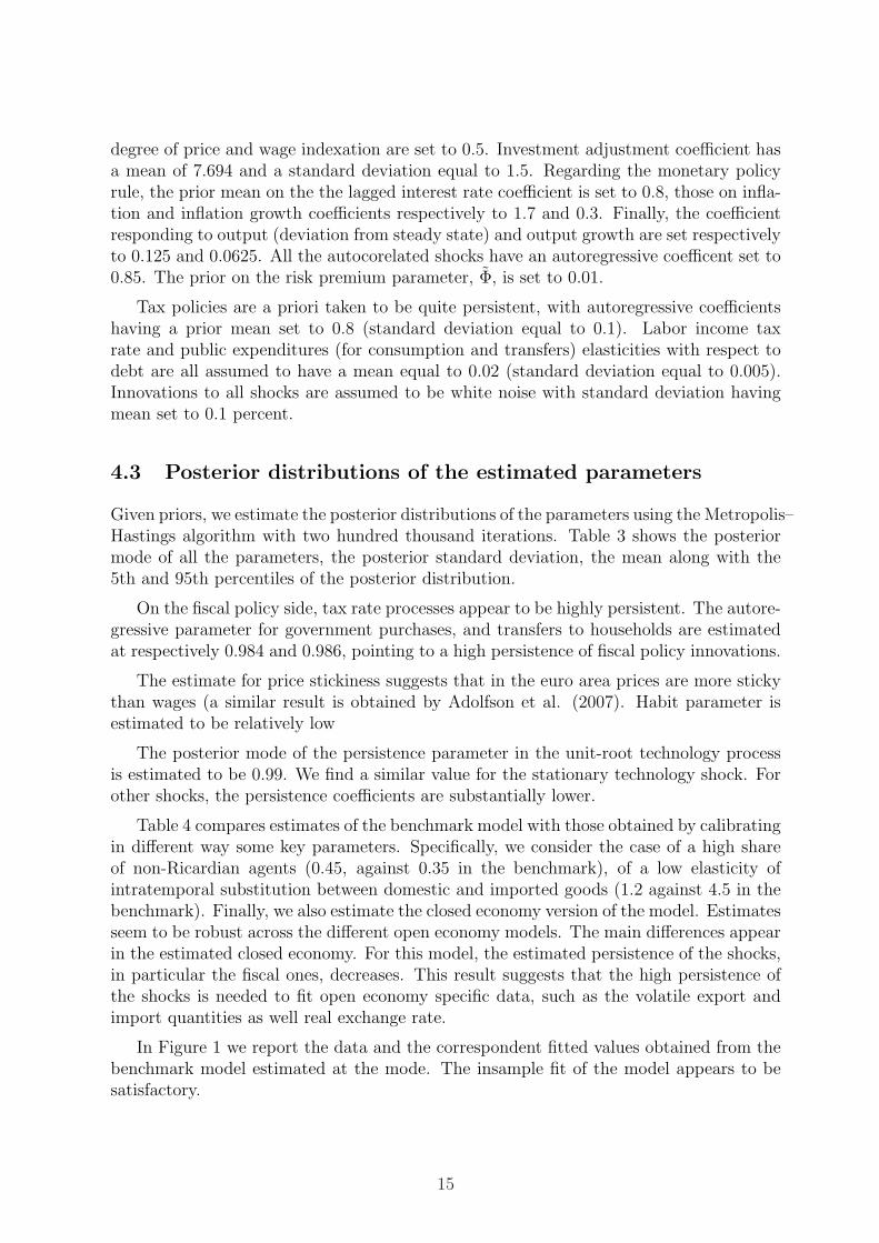
degree of price and wage indexation are set to 0.5. Investment adjustment coefficient hasa mean of 7.694 and a standard deviation equal to 1.5. Regarding the monetary policyrule, the prior mean on the the lagged interest rate coefficient is set to 0.8, those on infla-tion and inflation growth coefficients respectively to 1.7 and 0.3. Finally, the coefficientresponding to output (deviation from steady state) and output growth are set respectivelyto 0.125 and 0.0625. All the autocorelated shocks have an autoregressive coefficent set to0.85. The prior on the risk premium parameter, Φ, is set to 0.01.
Tax policies are a priori taken to be quite persistent, with autoregressive coefficientshaving a prior mean set to 0.8 (standard deviation equal to 0.1). Labor income taxrate and public expenditures (for consumption and transfers) elasticities with respect todebt are all assumed to have a mean equal to 0.02 (standard deviation equal to 0.005).Innovations to all shocks are assumed to be white noise with standard deviation havingmean set to 0.1 percent.
4.3 Posterior distributions of the estimated parameters
Given priors, we estimate the posterior distributions of the parameters using the Metropolis–Hastings algorithm with two hundred thousand iterations. Table 3 shows the posteriormode of all the parameters, the posterior standard deviation, the mean along with the5th and 95th percentiles of the posterior distribution.
On the fiscal policy side, tax rate processes appear to be highly persistent. The autore-gressive parameter for government purchases, and transfers to households are estimatedat respectively 0.984 and 0.986, pointing to a high persistence of fiscal policy innovations.
The estimate for price stickiness suggests that in the euro area prices are more stickythan wages (a similar result is obtained by Adolfson et al. (2007). Habit parameter isestimated to be relatively low
The posterior mode of the persistence parameter in the unit-root technology processis estimated to be 0.99. We find a similar value for the stationary technology shock. Forother shocks, the persistence coefficients are substantially lower.
Table 4 compares estimates of the benchmark model with those obtained by calibratingin different way some key parameters. Specifically, we consider the case of a high shareof non-Ricardian agents (0.45, against 0.35 in the benchmark), of a low elasticity ofintratemporal substitution between domestic and imported goods (1.2 against 4.5 in thebenchmark). Finally, we also estimate the closed economy version of the model. Estimatesseem to be robust across the different open economy models. The main differences appearin the estimated closed economy. For this model, the estimated persistence of the shocks,in particular the fiscal ones, decreases. This result suggests that the high persistence ofthe shocks is needed to fit open economy specific data, such as the volatile export andimport quantities as well real exchange rate.
In Figure 1 we report the data and the correspondent fitted values obtained from thebenchmark model estimated at the mode. The insample fit of the model appears to besatisfactory.
15

5 Impulse response Functions
5.1 Public expenditure shocks
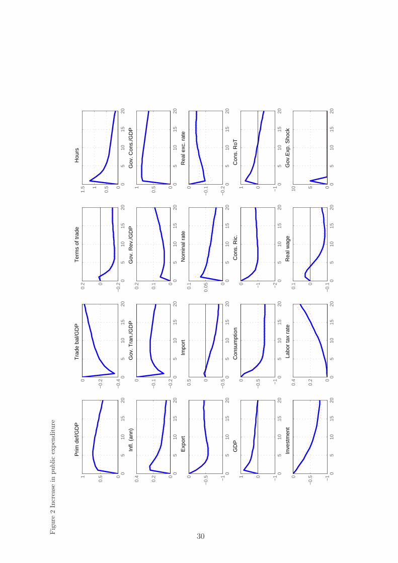
We now discuss the implications of our estimates for the effects of government spendingshocks on the economy, in particular on the trade balance and the public deficit. Fig. 2shows impulse responses with respect to a shock to real detrended government purchasesof goods and services while Fig. 3 with respect to real detrended transfers. The solidline shows median values, while the dotted ones the 5th and 95th percentile based onposterior distributions. The magnitude of the shocks is set in order to have an increase inexpenditures equal to one percent of steady state output. Impulse responses are expressedas percent deviation from steady state values. The exceptions are the interest rate andthe inflation rate, expressed as annualized percentage points, and fiscal and trade balancereported as a ratio to domestic steady state output (percentage points from steady state).
The shock to public government purchases (Figure 2) increases employment by in-creasing the demand for goods and services which, in turn, brings about an increase inlabor income. This sustains consumption of non-Ricardian households, to an extent that,however, is not enough (also in view of their share) to compensate for the decrease in Ri-cardian consumption due to the negative wealth effect of debt-financed spending and thehigher real interest rates (that crowds out also investment). On impact, the governmentspending multiplier does not exceeds unity.
The higher public expenditure implies an initial increase in the government budgetdeficit by about 0.6 percentage point of GDP. After the initial period, the deficit graduallydecreases, because labor income taxes and transfer adjust to make the public debt stable.
Imports decrease, following the decrease in the home private demand. The publicexpenditure is fully biased towards the domestic good, so its increase induces an improve-ment in the home terms of trade and the appreciation of the real exchange rate. Theincrease in the home goods relative prices favors a decrease in export. The trade deficit-to-GDP ratio deteriorates by about 0.4 percentage points in the first quarter (the peaklevel). Overall, the effect of public deficit on the external balance is rather strong.
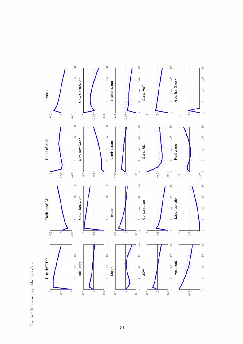
Figure 3 reports the effects of a shock to transfers to households. It has a big andpersistent impact on consumption as it translates one to one into an increase in dispos-able income of non-Ricardian households. Demand-driven output and employment alsoincrease, while real wages are initially unchanged. Higher labor effort stimulates physicalcapital accumulation and hence investment. Consumption and capital accumulation byRicardian agents decrease, because of the negative wealth effect of debt-financed spending(due to distortionary taxation) and to higher real interest rate. The higher public transferimplies an initial increase in the government budget deficit by about 0.8 percentage pointof GDP on impact. Subsequently, the deficit decreases very slowly.
Higher private consumption favors higher demand for domestic goods and higher im-ports. The trade balance-to-output ratio response is instead, differently from the case ofthe shock to government purchases, rather muted (around 0.1 percent). The higher pri-
16
vate aggregate demand induces an increase in imports and an improvement in the termsof trade (consistently with the exchange rate depreciation, given the assumption of localcurrency pricing and incomplete pass-through in the short run).
5.2 Shocks to tax rates
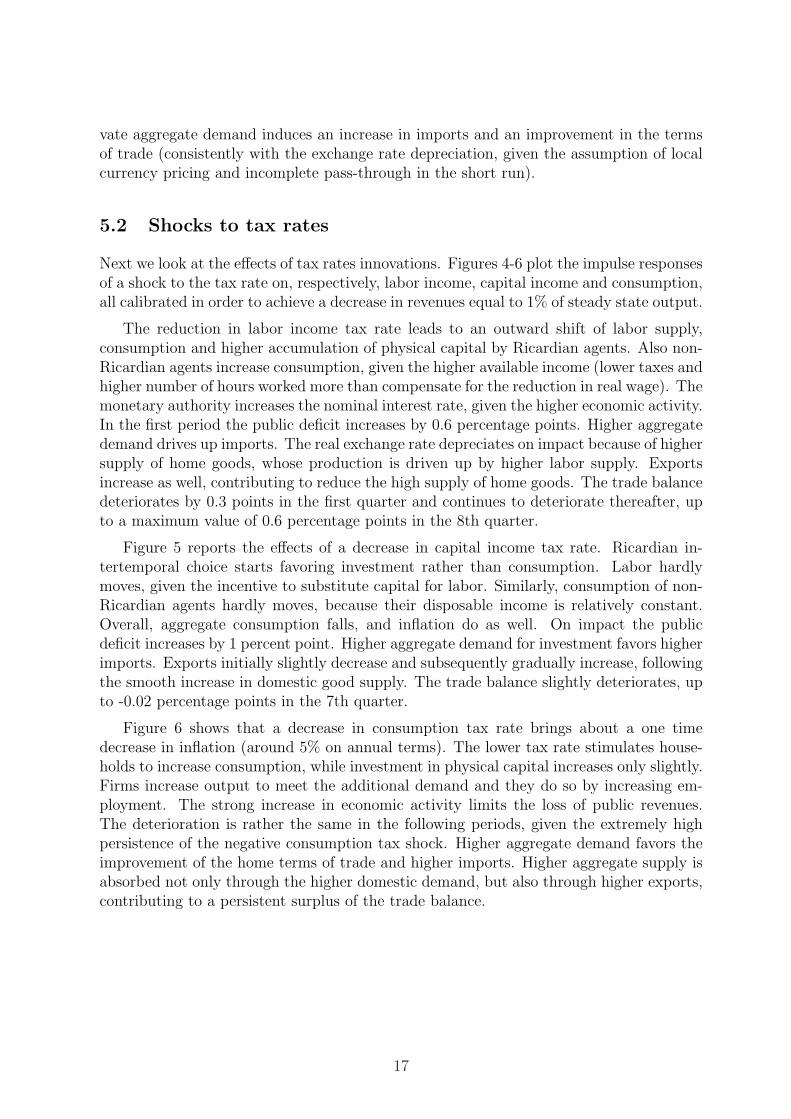
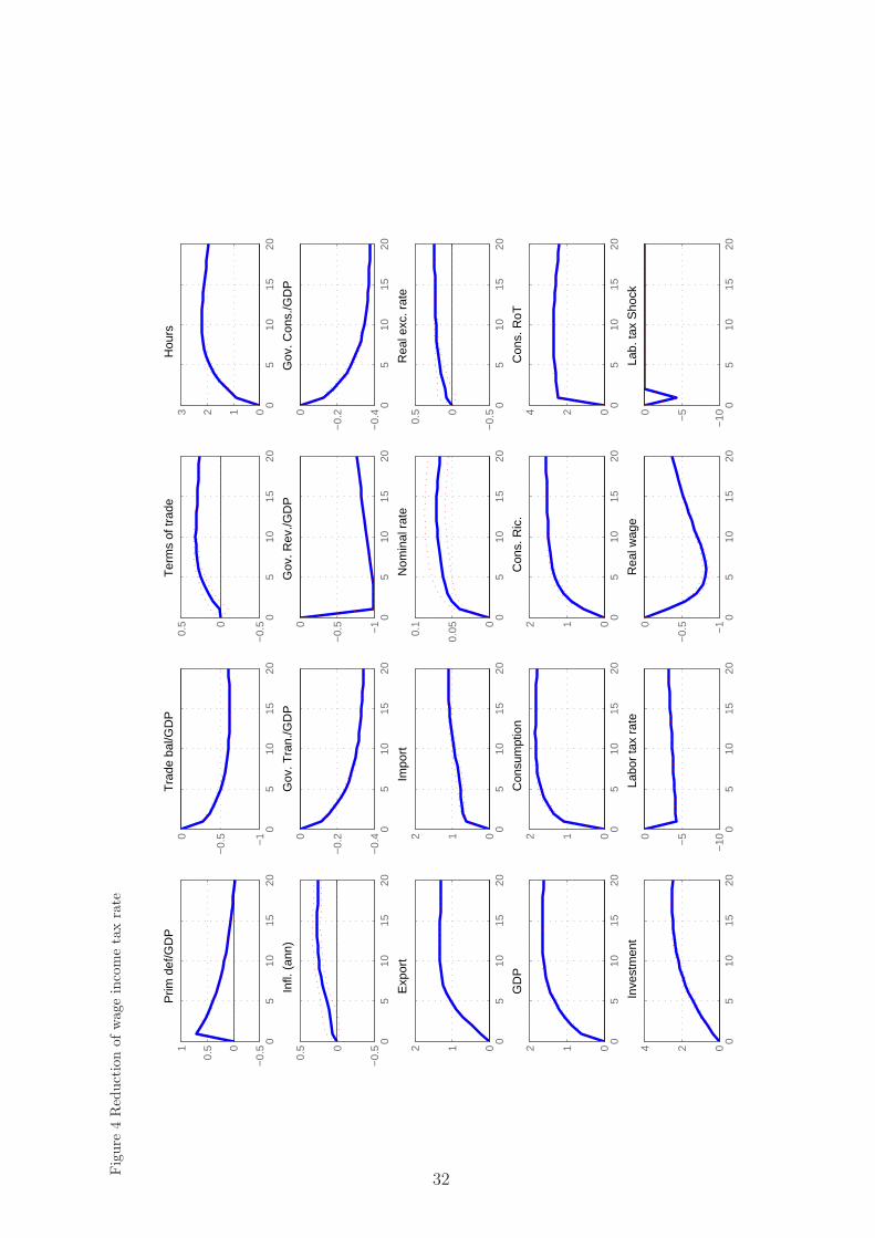
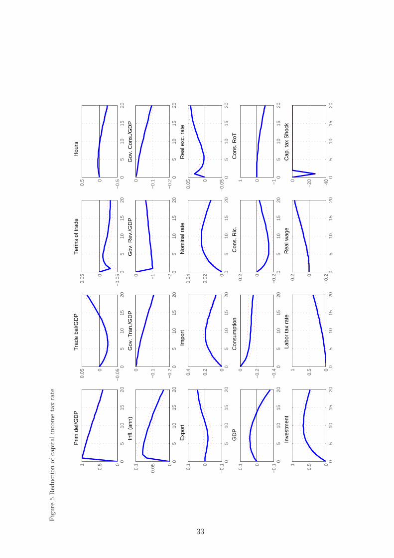
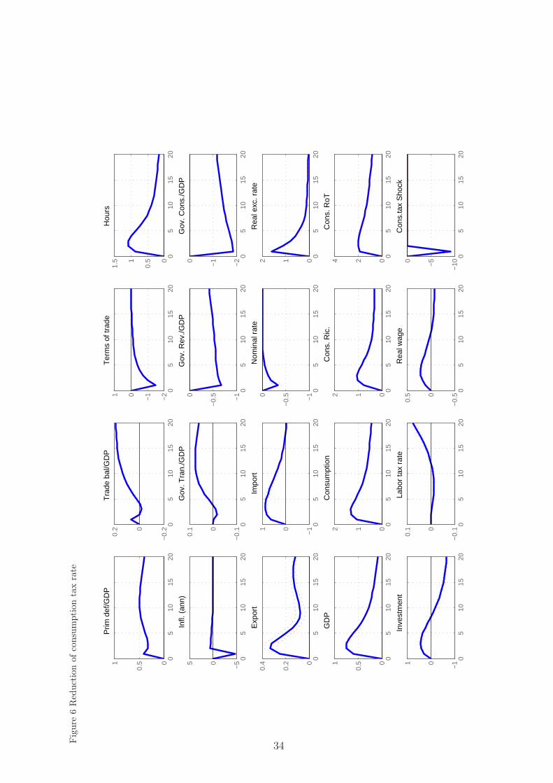
Next we look at the effects of tax rates innovations. Figures 4-6 plot the impulse responsesof a shock to the tax rate on, respectively, labor income, capital income and consumption,all calibrated in order to achieve a decrease in revenues equal to 1% of steady state output.
The reduction in labor income tax rate leads to an outward shift of labor supply,consumption and higher accumulation of physical capital by Ricardian agents. Also non-Ricardian agents increase consumption, given the higher available income (lower taxes andhigher number of hours worked more than compensate for the reduction in real wage). Themonetary authority increases the nominal interest rate, given the higher economic activity.In the first period the public deficit increases by 0.6 percentage points. Higher aggregatedemand drives up imports. The real exchange rate depreciates on impact because of highersupply of home goods, whose production is driven up by higher labor supply. Exportsincrease as well, contributing to reduce the high supply of home goods. The trade balancedeteriorates by 0.3 points in the first quarter and continues to deteriorate thereafter, upto a maximum value of 0.6 percentage points in the 8th quarter.
Figure 5 reports the effects of a decrease in capital income tax rate. Ricardian in-tertemporal choice starts favoring investment rather than consumption. Labor hardlymoves, given the incentive to substitute capital for labor. Similarly, consumption of non-Ricardian agents hardly moves, because their disposable income is relatively constant.Overall, aggregate consumption falls, and inflation do as well. On impact the publicdeficit increases by 1 percent point. Higher aggregate demand for investment favors higherimports. Exports initially slightly decrease and subsequently gradually increase, followingthe smooth increase in domestic good supply. The trade balance slightly deteriorates, upto -0.02 percentage points in the 7th quarter.
Figure 6 shows that a decrease in consumption tax rate brings about a one timedecrease in inflation (around 5% on annual terms). The lower tax rate stimulates house-holds to increase consumption, while investment in physical capital increases only slightly.Firms increase output to meet the additional demand and they do so by increasing em-ployment. The strong increase in economic activity limits the loss of public revenues.The deterioration is rather the same in the following periods, given the extremely highpersistence of the negative consumption tax shock. Higher aggregate demand favors theimprovement of the home terms of trade and higher imports. Higher aggregate supply isabsorbed not only through the higher domestic demand, but also through higher exports,contributing to a persistent surplus of the trade balance.
17

5.3 Fiscal multipliers
To summarize the quantitative effects of our five fiscal shocks we report in Table 5 thefiscal multipliers on output, consumption, investment, imports, exports, real exchangerate and inflation implied by our estimates. We report the average effects in the first1 and 4 quarters (first two lines) and from 4th to 8th quarters (third line) respectively,expressed in percentage points (annualized in the case of inflation).
Fiscal multipliers on output and consumption are quite sizeable, although generallysmaller than one. The average effect on output in the first quarter is, as expected, greatestfor a shock to purchases of good and services (these being part of aggregate demand); theother shocks all have multipliers between zero and 0.6. The effect on private consumptionis higher for innovations to consumption taxes, labor taxes and transfers. The effect, inall cases, works through an increase in household real income (this is true in particularfor non-Ricardian agents). For Ricardian agents an intertemporal substitution effect is atwork in the case of consumption and labor taxes.
The fiscal multipliers on imports mimics the multiplier on consumption and invest-ment, depending on the considered fiscal shock. The highest value is reached in corre-spondence of shocks to labour income tax, consumption tax and transfer (that stimulatesprivate consumption). The effect is somewhat smaller for capital income (that stimulatesprivate investment). The effects on the real exchange rate and inflation are generally mild.The only notable exception are the innovations in consumption taxes, as they translateone to one to prices and therefore affect strongly the real exchange rate.
6 Sensitivity Analysis
We have performed sensitivity by looking at the impulse responses to our fiscal shocksallowing one single parameter to move at a time while leaving the other parameters setat their estimated values. We focused on the following parameters: among calibratedones, the share of non-Ricardians and the elasticity of intratemporal substitution be-tween domestic and imported goods; among estimated one, the parameters of the fiscaland monetary rules (in particular, the persistence of the Fiscal rules). These are theparameters that most can impact on private consumption, and therefore imports, and onthe composition of final demand in domestically produced and imported goods.
Overall results are robust to variations in these parameters within reasonable bounds.Two relevant cases, that we discuss below, are the effect of the share of non-Ricardianconsumers on domestic consumption and imports (and therefore trade balance) and theresponse of the real exchange rate for values of the elasticity of intratemporal substitutionbetween domestic and imported goods higher that the one we assume. We will discussthese two cases with reference to a government expenditure shock.
Figure 7 reports the impact responses of private consumption, investment and imports(upper panel), and of the terms of trade and real exchange rate (lower panel) following agovernment expenditure shock for values of λNR between zero and one. The response of
18

consumption and imports is significantly increasing in the share of non-Ricardian agents.Note that the consumption response becomes positive for values of λ around 0.5. Con-sistently with the response of domestic consumption, that induce a stronger increase indemand for domestic goods, the terms of trade appreciates to a bigger extent and the realexchange rate appreciates less.
Figure 8 shows the response to a government expenditure shock of the same variables,now moving the value of the elasticity of substitution between domestic tradables andimported goods. The impact responses highlight that real variables (consumption, in-vestment and imports) tend to remain relatively stable, while the relative prices (termsof trade and real exchange rate) move significantly. In particular, the real exchange rateappreciate less. When we also assume that the expenditure shock is not very persistent -as in the figure where we set ρG=0.8 - then we can have also that the real exchange ratedepreciates for values of the elasticity approximately higher than 4.5. This is interesting,as we have already discussed that several authors have found evidence in favour of a depre-ciation of the real exchange rate following an expenditure shock, although with referenceto US data. The figure shows that the model we are considering allows in principle fordepreciations after an expenditure shock, although our estimates does not find supportfor this result.
Figure 9 shows the responses to a spending shock for values of the persistence ofthe fiscal shock (ρG) between 0.8 and 1. A more persistent process produces a strongernegative wealth effect on Ricardian agents that drives down imports. The exchange rateappreciate less.
Finally the response of variables is inversely proportional to the tightness of monetarypolicy. These effects however are not very strong and therefore we do not show anyparticular figure on this point. Higher consumption and import responses are obtainedwhen the coefficient of response to CPI inflation in the Taylor rule is low, so that there isa lower reaction of the nominal interest rate to the fiscal stimulus (so the increase in thereal interest rate is lower, and the implied depressing effect on Ricardian aggregate effectis lower as well).
7 Conclusions
TO BE WRITTEN
19
References
[1] Adolfson, M., Laseen, S., Linde, J., Villani, M., 2005. Bayesian estimation of anopen economy DSGE model with incomplete pass-through. Working Paper, vol. 179.Sveriges Riksbank.
[2] Adolfson, M., Laseen, S., Linde, J., Villani, M., 2006. Appendix to: Bayesian Estima-tion of an Open Economy DSGE Model with Incomplete Pass-Through. Manuscript.Sveriges Riksbank.
[3] Adolfson, M., Linde, J., Villani, M., in press. Forecasting performance of an openeconomy DSGE model, Econometric Reviews. Working Paper, vol. 190. SverigesRiksbank.
[4] Altig, D., Christiano, L.J., Eichenbaum, M., Linde, J., 2003. The Role of MonetaryPolicy in the Propagation of Technology Shocks. Manuscript. Northwestern Univer-sity.
[5] Altig, D., Christiano, L.J., Eichenbaum, M., Linde, J., 2004. Firm-specific capital,nominal rigidities and the business cycle. Working Paper, vol. 176. Sveriges Riks-bank..
[6] Bouakez, H., 2005. Nominal rigidity, desired markup variations, and real exchangerate persistence. Journal of International Economics 66 (1), 49–74.
[7] Calvo, G., 1983. Staggered prices in a utility maximizing framework. Journal ofMonetary Economics 12, 383–398.
[8] Christiano, L.J., Eichenbaum, M., Evans, C., 2005. Nominal rigidities and the dy-namic effects of a shock to monetary policy. Journal of Political Economy 113 (1),1–45.
[9] Devereux, M.B., Engel, C., 2002. Exchange rate pass-through, exchange rate volatil-ity and exchange rate disconnect. Journal of Monetary Economics 49 (4), 913–940.
[10] Duarte, M., Stockman, A.C., 2005. Rational speculation and exchange rates. Journalof Monetary Economics 52, 3–29.
[11] Eichenbaum, M., Evans, C., 1995. Some empirical evidence on the effects of shocks tomonetary policy on exchange rates. Quarterly Journal of Economics 110, 975–1010.
[12] Erceg, C., Henderson, D., Levin, A., 2000. Optimal monetary policy with staggeredwage and price contracts. Journal of Monetary Economics 46 (2), 281–313.
[13] Fagan, G., Henry, J., Mestre, R., 2005. An area-wide model for the Euro area. Eco-nomic Modelling 22 (1), 39–59.
[14] Faust, J., Rogers, J.H., 2003. Monetary policy’s role in exchange rate behavior. Jour-nal of Monetary Economics 50, 1403–1424.
20
[15] Forni, L., Monteforte, L., Sessa, L. 2009. The general equilibrium effects of fiscalpolicy: estimates for the Euro area. Journal of Public Economics 93, 559–585.
[16] Fuhrer, J., Moore, G., 1995. Inflation persistence. Quarterly Journal of EconomicsCX, 127–160.
[17] Galı, J., Monacelli, T., 2005. Monetary policy and exchange rate volatility in a smallopen economy. Review of Economic Studies 72 (3), 707–734 (July).
[18] Galı, J., Gertler, M., Lopez-Salido, D., 2001. European inflation dynamics. EuropeanEconomic Review 45 (7), 1237–1270.
[19] Gelman, A., Carlin, J., Stern, H., Rubin, D., 2004. Bayesian Data Analysis, 2ndedition. Chapman and Hall, New York.
[20] Geweke, J., 1999. Using simulation methods for Bayesian econometrics models: in-ference, development and communication. Econometric Reviews 18 (1), 1–73.
[21] Hamilton, J., 1994. Times Series Analysis. Princeton University Press.
[22] Justiniano, A., Preston, B., 2004. Small Open Economy DSGE Models: Specification,Estimation and Model Fit. manuscript. Columbia University.
[23] Kollmann, R., 2001. The exchange rate in a dynamic-optimizing business cycle modelwith nominal rigidities: a quantitative investigation. Journal of International Eco-nomics 55, 243–262.
[24] Linde, J., 2003. Comment on the output composition puzzle: a difference in themonetary transmission mechanism in the Euro area and U.S. by Angeloni, I., Kasyap,A.K., Mojon, B. and D. Terlizzese. Journal of Money, Credit and Banking 35 (6),1309–1318.
[25] Linde, J., Nessen, M., Soderstrom, U., 2003. Monetary Policy in an Estimated Open-Economy Model with Imperfect Pass-Through. Working Paper, vol. 167. SverigesRiksbank.
[26] Lubik, T., Schorfheide, F., 2005. A Bayesian look at new open economy macroeco-nomics. In: Gertler, M., Rogoff, K. (Eds.), NBER Macroeconomics Annual. MITPress.
[27] Lundvik, P., 1992. Foreign demand and domestic business cycles: Sweden 1891–1987, chapter 3 in business cycles and growth. Monograph Series, vol. 22. Institutefor International Economic Studies, Stockholm University.
[28] Mash, R., 2004. Optimising microfoundations for inflation persistence. Working Pa-per, vol. 183. University of Oxford.
[29] Obstfeld, M., Rogoff, K., 2000. The six major puzzles in international macroeco-nomics: is there a common cause? In: Bernanke, B., Rogoff, K. (Eds.), NBERMacroeconomics Annual. MIT Press.
21

[30] Onatski, A., Williams, N., 2004. Empirical and Policy Performance of a Forward-Looking Monetary Model. Manuscript. Princeton University.
[31] Rabanal, P., Tuesta, V., 2006. Euro–Dollar real exchange rare dynamics in an esti-mated two-country model: what is important and what is not? Working Paper, vol.06/177. International Monetary Fund.
[32] Rotemberg, J.J., 1982. Monopolistic price adjustment and aggregate output. Reviewof Economic Studies 49, 517–531.
[33] Schmitt-Grohe, S., Uribe, M., 2001. Stabilization policy and the cost of dollarization.Journal of Money, Credit and Banking 33 (2), 482–509.
[34] Schorfheide, F., 2000. Loss function-based evaluation of DSGE models. Journal ofApplied Econometrics 15 (6), 645–670.
[35] Smets, F., Wouters, R., 2002. Openness, imperfect exchange rate pass-through andmonetary policy. Journal of Monetary Economics 49 (5), 913–940.
[36] Smets, F., Wouters, R., 2003. An estimated dynamic stochastic general equilibriummodel of the Euro area. Journal of the European Economic Association 1 (5), 1123–1175.
[37] Smets, F., Wouters, R., 2005. Comparing shocks and frictions in US and Euro areaBusiness cycles: a Bayesian DSGE approach. Journal of Applied Econometrics 20(2), 161–183.
[38] Woodford, M., 2003. Interest and Prices: Foundations of a Theory of MonetaryPolicy. Princeton University Press, Princeton.
22
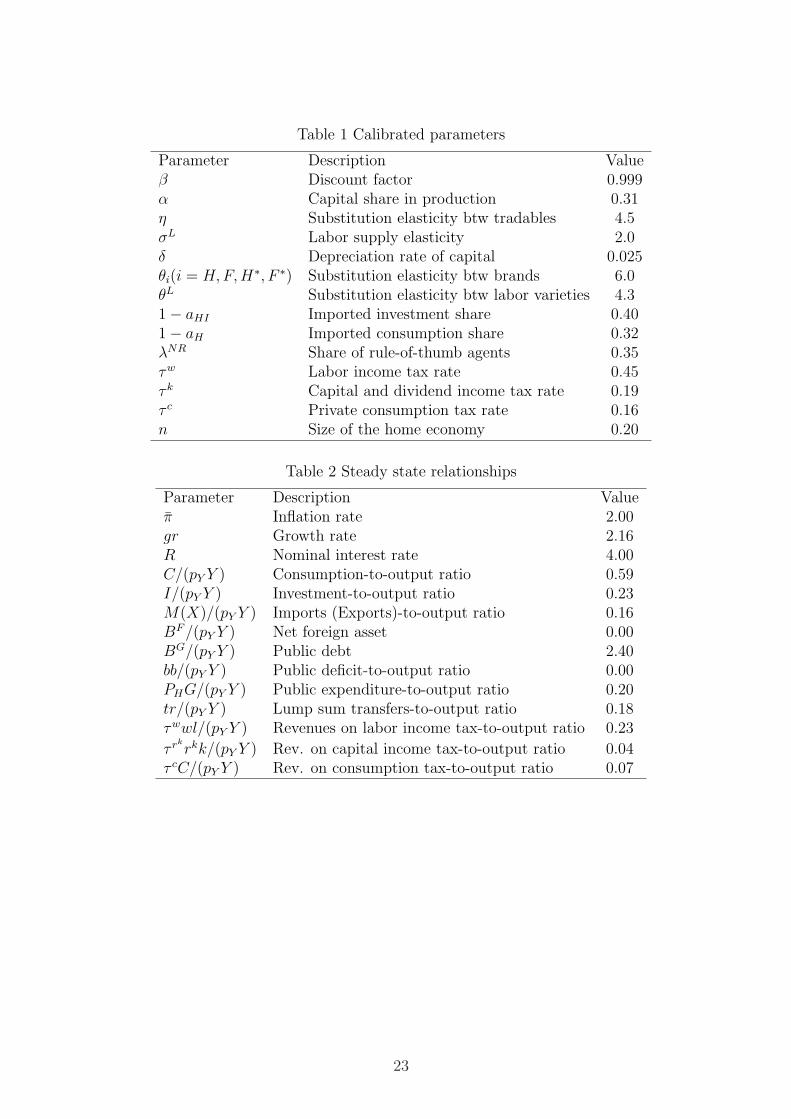
Table 1 Calibrated parameters
Parameter Description Valueβ Discount factor 0.999α Capital share in production 0.31η Substitution elasticity btw tradables 4.5σL Labor supply elasticity 2.0δ Depreciation rate of capital 0.025θi(i = H,F,H∗, F ∗) Substitution elasticity btw brands 6.0θL Substitution elasticity btw labor varieties 4.31− aHI Imported investment share 0.401− aH Imported consumption share 0.32λNR Share of rule-of-thumb agents 0.35τw Labor income tax rate 0.45τ k Capital and dividend income tax rate 0.19τ c Private consumption tax rate 0.16n Size of the home economy 0.20
Table 2 Steady state relationships
Parameter Description Valueπ Inflation rate 2.00gr Growth rate 2.16R Nominal interest rate 4.00C/(pY Y ) Consumption-to-output ratio 0.59I/(pY Y ) Investment-to-output ratio 0.23M(X)/(pY Y ) Imports (Exports)-to-output ratio 0.16BF /(pY Y ) Net foreign asset 0.00BG/(pY Y ) Public debt 2.40bb/(pY Y ) Public deficit-to-output ratio 0.00PHG/(pY Y ) Public expenditure-to-output ratio 0.20tr/(pY Y ) Lump sum transfers-to-output ratio 0.18τwwl/(pY Y ) Revenues on labor income tax-to-output ratio 0.23
τ rkrkk/(pY Y ) Rev. on capital income tax-to-output ratio 0.04
τ cC/(pY Y ) Rev. on consumption tax-to-output ratio 0.07
23
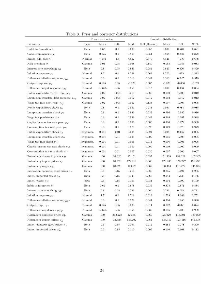
Table 3. Prior and posterior distributionsPrior distribution Posterior distribution
Parameter Type Mean S.D. Mode S.D.(Hessian) Mean 5 % 95 %
Habit in formation b Beta 0.65 0.1 0.600 0.055 0.600 0.578 0.621
Calvo employment ξE Beta 0.675 0.1 0.869 0.054 0.868 0.858 0.878
Invest. adj. cost γI Normal 7.694 1.5 8.507 0.079 8.521 7.536 9.638
Risk premium Φ Gamma 0.01 0.05 0.068 0.149 0.068 0.053 0.083
Interest rate smoothing ρR Beta 0.8 0.05 0.843 0.081 0.843 0.826 0.859
Inflation response ρπ Normal 1.7 0.1 1.768 0.063 1.773 1.675 1.873
Difference inflation response ρ∆π Normal 0.3 0.1 0.313 0.042 0.313 0.247 0.379
Output response ρy Normal 0.125 0.05 -0.028 0.005 -0.028 -0.036 -0.021
Difference output response ρ∆y Normal 0.0625 0.05 0.059 0.015 0.060 0.036 0.084
Public expenditure debt resp. ηGbGamma 0.02 0.005 0.010 0.085 0.010 0.009 0.012
Lump-sum transfers debt response ηtrb Gamma 0.02 0.005 0.012 0.012 0.012 0.012 0.012
Wage tax rate debt resp. ητwb
Gamma 0.02 0.005 0.007 0.133 0.007 0.005 0.008
Public expenditure shock ρg Beta 0.8 0.1 0.984 0.033 0.984 0.983 0.985
Lump-sum transfers shock ρtr Beta 0.8 0.1 0.986 0.033 0.986 0.985 0.986
Wage tax persistence ρτw Beta 0.8 0.1 0.988 0.042 0.988 0.987 0.988
Capital income tax rate pers. ρτk Beta 0.8 0.1 0.980 0.006 0.980 0.979 0.980
Consumption tax rate pers. ρτc Beta 0.8 0.1 0.979 0.020 0.979 0.978 0.979
Public expenditure shock σg Invgamma 0.001 0.01 0.005 0.021 0.005 0.005 0.005
Lump-sum transfers shock σtr Invgamma 0.001 0.01 0.005 0.009 0.005 0.005 0.005
Wage tax rate shock στw Invgamma 0.001 0.01 0.006 0.016 0.006 0.006 0.006
Capital income tax rate shock στk Invgamma 0.001 0.01 0.009 0.009 0.009 0.009 0.009
Consumption tax rate shock στc Invgamma 0.001 0.01 0.007 0.020 0.007 0.006 0.007
Rotemberg domestic prices κH Gamma 100 31.623 151.51 0.057 151.528 138.329 165.305
Rotemberg import prices κF Gamma 100 31.623 172.919 0.060 173.836 158.247 191.230
Rotemberg wages κW Gamma 100 31.623 129.97 0.069 130.364 116.272 145.324
Indexation domestic good prices αH Beta 0.5 0.15 0.216 0.080 0.215 0.194 0.235
Index. imported prices αF Beta 0.5 0.15 0.143 0.060 0.144 0.133 0.156
Index. wages αW beta 0.5 0.15 0.104 0.034 0.104 0.099 0.109
habit in formation b∗ Beta 0.65 0.1 0.878 0.036 0.878 0.871 0.884
Interest rate smoothing ρR∗ Beta 0.8 0.05 0.753 0.060 0.753 0.735 0.771
Inflation response ρπ∗ Normal 1.7 0.1 1.718 0.019 1.719 1.688 1.751
Difference inflation response ρ∆π∗ Normal 0.3 0.1 0.329 0.044 0.326 0.256 0.396
Output resp. ρy∗ Normal 0.125 0.05 0.003 0.014 0.002 -0.021 0.024
Difference output resp. ρ∆y∗ Normal 0.0625 0.05 0.156 0.032 0.156 0.105 0.208
Rotemberg domestic prices κ∗F Gamma 100 31.6228 125.35 0.069 125.929 113.001 139.299
Rotemberg import prices κ∗H Gamma 100 31.623 136.202 0.061 136.357 123.416 149.438
Index. domestic good prices α∗F Beta 0.5 0.15 0.284 0.016 0.284 0.278 0.290
Index. imported prices α∗H Beta 0.5 0.15 0.110 0.009 0.110 0.108 0.112
24
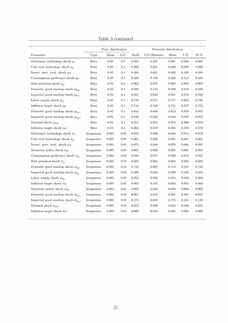
Table 3 continued
Prior distribution Posterior distribution
Parameter Type Mean S.D. Mode S.D.(Hessian) Mean 5 % 95 %
Stationary technology shock ρε Beta 0.85 0.1 0.991 0.237 0.991 0.988 0.994
Unit root technology shock ρµ Beta 0.85 0.1 0.989 0.051 0.989 0.988 0.990
Invest. spec. tech. shock ρΥ Beta 0.85 0.1 0.463 0.061 0.462 0.438 0.485
Consumption preference shock ρξc Beta 0.85 0.1 0.928 0.150 0.928 0.912 0.943
Risk premium shock ρφ Beta 0.85 0.1 0.963 0.072 0.963 0.959 0.967
Domestic good markup shock ρθHBeta 0.85 0.1 0.928 0.112 0.928 0.916 0.940
Imported good markup shock ρθFBeta 0.85 0.1 0.921 0.042 0.921 0.916 0.926
Labor supply shock ρθLBeta 0.85 0.1 0.716 0.071 0.717 0.694 0.740
Inflation target shock ρπ Beta 0.85 0.1 0.744 0.109 0.741 0.707 0.772
Domestic good markup shock ρθF∗ Beta 0.85 0.1 0.852 0.008 0.853 0.850 0.855
Imported good markup shock ρθH∗ Beta 0.85 0.1 0.949 0.029 0.949 0.947 0.952
Demand shock ρad∗ Beta 0.85 0.1 0.913 0.051 0.913 0.906 0.919
Inflation target shock ρπ∗ Beta 0.85 0.1 0.364 0.013 0.365 0.359 0.370
Stationary technology shock σε Invgamma 0.001 0.01 0.016 0.086 0.016 0.014 0.018
Unit root technology shock σµ Invgamma 0.001 0.01 0.001 0.026 0.001 0.001 0.001
Invest. spec. tech. shock σΥ Invgamma 0.001 0.01 0.075 0.086 0.076 0.066 0.087
Monetary policy shock σR Invgamma 0.001 0.01 0.001 0.026 0.001 0.001 0.001
Consumption preference shock σξc Invgamma 0.001 0.01 0.020 0.057 0.020 0.018 0.022
Risk premium shock σφ Invgamma 0.001 0.01 0.004 0.064 0.004 0.003 0.004
Domestic good markup shock σθHInvgamma 0.001 0.01 0.112 0.063 0.112 0.101 0.123
Imported good markup shock σθFInvgamma 0.001 0.01 0.208 0.048 0.208 0.192 0.224
Labor supply shock σθLInvgamma 0.001 0.01 0.054 0.058 0.054 0.049 0.060
Inflation target shock σπ Invgamma 0.001 0.01 0.002 0.107 0.002 0.002 0.003
Monetary policy shock σR∗ Invgamma 0.001 0.01 0.002 0.024 0.002 0.002 0.002
Domestic good markup shock σθF∗ Invgamma 0.001 0.01 0.001 0.012 0.001 0.001 0.001
Imported good markup shock σθH∗ Invgamma 0.001 0.01 0.174 0.048 0.175 0.161 0.188
Demand shock σad∗ Invgamma 0.001 0.01 0.052 0.036 0.052 0.049 0.055
Inflation target shock σπ∗ Invgamma 0.001 0.01 0.005 0.024 0.005 0.004 0.005
25
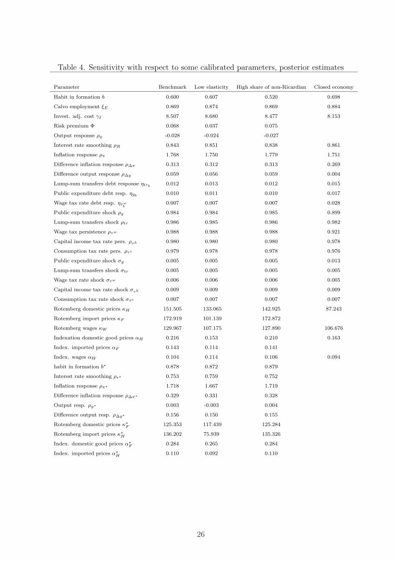
Table 4. Sensitivity with respect to some calibrated parameters, posterior estimates
Parameter Benchmark Low elasticity High share of non-Ricardian Closed economy
Habit in formation b 0.600 0.607 0.520 0.698
Calvo employment ξE 0.869 0.874 0.869 0.884
Invest. adj. cost γI 8.507 8.680 8.477 8.153
Risk premium Φ 0.068 0.037 0.075
Output response ρy -0.028 -0.024 -0.027
Interest rate smoothing ρR 0.843 0.851 0.838 0.861
Inflation response ρπ 1.768 1.750 1.779 1.751
Difference inflation response ρ∆π 0.313 0.312 0.313 0.269
Difference output response ρ∆y 0.059 0.056 0.059 0.004
Lump-sum transfers debt response ηtrb 0.012 0.013 0.012 0.015
Public expenditure debt resp. ηgb 0.010 0.011 0.010 0.017
Wage tax rate debt resp. ητwb
0.007 0.007 0.007 0.028
Public expenditure shock ρg 0.984 0.984 0.985 0.899
Lump-sum transfers shock ρtr 0.986 0.985 0.986 0.982
Wage tax persistence ρτw 0.988 0.988 0.988 0.921
Capital income tax rate pers. ρτk 0.980 0.980 0.980 0.978
Consumption tax rate pers. ρτc 0.979 0.978 0.978 0.976
Public expenditure shock σg 0.005 0.005 0.005 0.013
Lump-sum transfers shock σtr 0.005 0.005 0.005 0.005
Wage tax rate shock στw 0.006 0.006 0.006 0.005
Capital income tax rate shock στk 0.009 0.009 0.009 0.009
Consumption tax rate shock στc 0.007 0.007 0.007 0.007
Rotemberg domestic prices κH 151.505 133.065 142.925 87.243
Rotemberg import prices κF 172.919 101.139 172.872
Rotemberg wages κW 129.967 107.175 127.890 106.676
Indexation domestic good prices αH 0.216 0.153 0.210 0.163
Index. imported prices αF 0.143 0.114 0.141
Index. wages αW 0.104 0.114 0.106 0.094
habit in formation b∗ 0.878 0.872 0.879
Interest rate smoothing ρr∗ 0.753 0.759 0.752
Inflation response ρπ∗ 1.718 1.667 1.719
Difference inflation response ρ∆π∗ 0.329 0.331 0.328
Output resp. ρy∗ 0.003 -0.003 0.004
Difference output resp. ρ∆y∗ 0.156 0.150 0.155
Rotemberg domestic prices κ∗F 125.353 117.439 125.284
Rotemberg import prices κ∗H 136.202 75.939 135.326
Index. domestic good prices α∗F 0.284 0.265 0.284
Index. imported prices α∗H 0.110 0.092 0.110
26
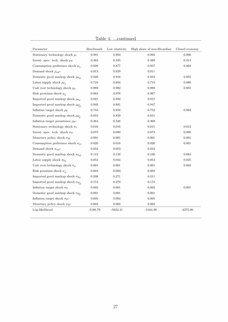
Table 4. ...continued
Parameter Benchmark Low elasticity High share of non-Ricardian Closed economy
Stationary technology shock ρε 0.991 0.994 0.992 0.996
Invest. spec. tech. shock ρΥ 0.463 0.435 0.489 0.214
Consumption preference shock ρζc 0.928 0.877 0.957 0.863
Demand shock ρad∗ 0.913 0.929 0.911
Domestic good markup shock ρθH0.928 0.916 0.934 0.935
Labor supply shock ρθL0.716 0.804 0.713 0.880
Unit root technology shock ρµ 0.989 0.992 0.988 0.885
Risk premium shock ρφ 0.963 0.978 0.967
Imported good markup shock ρθF0.921 0.892 0.915
Imported good markup shock ρθ∗H
0.949 0.881 0.947
Inflation target shock ρπ 0.744 0.858 0.752 0.994
Domestic good markup shock ρθ∗F
0.853 0.850 0.851
Inflation target persistence ρπ∗ 0.364 0.348 0.369
Stationary technology shock σε 0.016 0.016 0.015 0.012
Invest. spec. tech. shock σΥ 0.075 0.080 0.073 0.090
Monetary policy shock σR 0.001 0.001 0.001 0.001
Consumption preference shock σζc 0.020 0.018 0.020 0.001
Demand shock σad∗ 0.052 0.053 0.052
Domestic good markup shock σθH0.112 0.129 0.106 0.084
Labor supply shock σθL0.054 0.044 0.054 0.035
Unit root technology shock σµ 0.001 0.001 0.001 0.003
Risk premium shock σφ 0.004 0.003 0.004
Imported good markup shock σθF0.208 0.271 0.211
Imported good markup shock σθ∗H
0.174 0.279 0.174
Inflation target shock σπ 0.002 0.001 0.002 0.001
Domestic good markup shock σθ∗F
0.001 0.001 0.001
Inflation target shock σπ∗ 0.005 0.004 0.005
Monetary policy shock σR∗ 0.002 0.002 0.002
Log-likelihood -5180.79 -5622.41 -5164.39 -4275.96
27
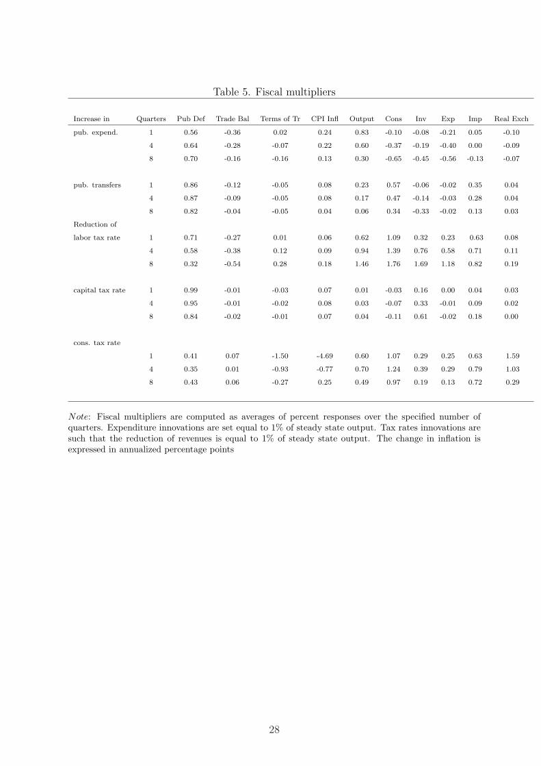
Table 5. Fiscal multipliers
Increase in Quarters Pub Def Trade Bal Terms of Tr CPI Infl Output Cons Inv Exp Imp Real Exch
pub. expend. 1 0.56 -0.36 0.02 0.24 0.83 -0.10 -0.08 -0.21 0.05 -0.10
4 0.64 -0.28 -0.07 0.22 0.60 -0.37 -0.19 -0.40 0.00 -0.09
8 0.70 -0.16 -0.16 0.13 0.30 -0.65 -0.45 -0.56 -0.13 -0.07
pub. transfers 1 0.86 -0.12 -0.05 0.08 0.23 0.57 -0.06 -0.02 0.35 0.04
4 0.87 -0.09 -0.05 0.08 0.17 0.47 -0.14 -0.03 0.28 0.04
8 0.82 -0.04 -0.05 0.04 0.06 0.34 -0.33 -0.02 0.13 0.03
Reduction of
labor tax rate 1 0.71 -0.27 0.01 0.06 0.62 1.09 0.32 0.23 0.63 0.08
4 0.58 -0.38 0.12 0.09 0.94 1.39 0.76 0.58 0.71 0.11
8 0.32 -0.54 0.28 0.18 1.46 1.76 1.69 1.18 0.82 0.19
capital tax rate 1 0.99 -0.01 -0.03 0.07 0.01 -0.03 0.16 0.00 0.04 0.03
4 0.95 -0.01 -0.02 0.08 0.03 -0.07 0.33 -0.01 0.09 0.02
8 0.84 -0.02 -0.01 0.07 0.04 -0.11 0.61 -0.02 0.18 0.00
cons. tax rate
1 0.41 0.07 -1.50 -4.69 0.60 1.07 0.29 0.25 0.63 1.59
4 0.35 0.01 -0.93 -0.77 0.70 1.24 0.39 0.29 0.79 1.03
8 0.43 0.06 -0.27 0.25 0.49 0.97 0.19 0.13 0.72 0.29
Note: Fiscal multipliers are computed as averages of percent responses over the specified number ofquarters. Expenditure innovations are set equal to 1% of steady state output. Tax rates innovations aresuch that the reduction of revenues is equal to 1% of steady state output. The change in inflation isexpressed in annualized percentage points
28
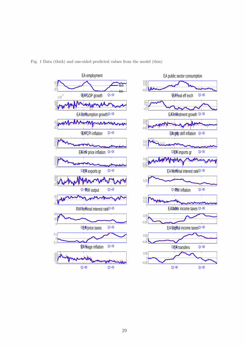
Fig. 1 Data (thick) and one-sided predicted values from the model (thin)
Q1−90 Q1−00
−0.020
0.02
EA employment
fitted
dataQ1−90 Q1−00
−0.020
0.020.04
EA public sector consumption
Q1−90 Q1−00−50
51015x 10
−3 EA GDP growth
Q1−90 Q1−00−0.1
00.10.2
EA real eff exch
Q1−90 Q1−00−0.01
00.01
EA consumption growth
Q1−90 Q1−00−0.02
00.020.04
EA investment growth
Q1−90 Q1−000
0.010.020.03
EA CPI inflation
Q1−90 Q1−000
0.010.02
EA gdp defl inflation
Q1−90 Q1−000
0.010.020.03
EA inv price inflation
Q1−90 Q1−00−0.04−0.02
00.02
EA imports gr
Q1−90 Q1−00−0.02
00.020.04
EA exports gr
Q1−90 Q1−000
0.02
EA nominal interest rate
Q1−90 Q1−00−0.01
00.01
RW output
Q1−90 Q1−000
0.010.02
RW inflation
Q1−90 Q1−000
0.020.04
RW nominal interest rate
Q1−90 Q1−00−0.05
00.05
EA labor income taxes
Q1−90 Q1−00−0.1
00.1
EA price taxes
Q1−90 Q1−00−0.05
00.05
EA capital income taxes
Q1−90 Q1−000
0.010.020.03
EA wage inflation
Q1−90 Q1−00−0.05
00.05
EA transfers
29
Fig
ure
2In
crea
sein
publ
icex
pend
itur
e
05
1015
200
0.51
Prim
def
/GD
P
05
1015
20−
0.4
−0.
20T
rade
bal
/GD
P
05
1015
20−
0.20
0.2
Ter
ms
of tr
ade
05
1015
200
0.51
1.5
Hou
rs
05
1015
200
0.2
0.4
Infl.
(an
n)
05
1015
20−
0.2
−0.
10G
ov. T
ran.
/GD
P
05
1015
200
0.1
0.2
Gov
. Rev
./GD
P
05
1015
200
0.51
Gov
. Con
s./G
DP
05
1015
20−
1
−0.
50E
xpor
t
05
1015
20−
0.50
0.5
Impo
rt
05
1015
200
0.050.1
Nom
inal
rat
e
05
1015
20−
0.2
−0.
10R
eal e
xc. r
ate
05
1015
20−
101G
DP
05
1015
20−
1
−0.
50C
onsu
mpt
ion
05
1015
20−
2
−10
Con
s. R
ic.
05
1015
20−
101C
ons.
RoT
05
1015
20−
1
−0.
50In
vest
men
t
05
1015
200
0.2
0.4
Labo
r ta
x ra
te
05
1015
20−
0.10
0.1
Rea
l wag
e
05
1015
200510
Gov
.Exp
. Sho
ck
30
Fig
ure
3In
crea
sein
publ
ictr
ansf
ers
05
1015
200
0.51
Prim
def
/GD
P
05
1015
20−
0.20
0.2
Tra
de b
al/G
DP
05
1015
20−
0.1
−0.
050T
erm
s of
trad
e
05
1015
20−
0.50
0.5
Hou
rs
05
1015
20−
0.20
0.2
Infl.
(an
n)
05
1015
200
0.51
Gov
. Tra
n./G
DP
05
1015
200
0.1
0.2
Gov
. Rev
./GD
P
05
1015
20−
0.1
−0.
050G
ov. C
ons.
/GD
P
05
1015
20−
0.10
0.1
Exp
ort
05
1015
20−
0.50
0.5
Impo
rt
05
1015
20−
0.050
0.05
Nom
inal
rat
e
05
1015
200
0.050.1
Rea
l exc
. rat
e
05
1015
20−
0.50
0.5
GD
P
05
1015
200
0.51
Con
sum
ptio
n
05
1015
20−
0.4
−0.
20C
ons.
Ric
.
05
1015
20024
Con
s. R
oT
05
1015
20−
1
−0.
50In
vest
men
t
05
1015
200
0.51
Labo
r ta
x ra
te
05
1015
20−
0.050
0.05
Rea
l wag
e
05
1015
200510
Gov
.Tra
. Sho
ck
31
Fig
ure
4R
educ
tion
ofw
age
inco
me
tax
rate
05
1015
20−
0.50
0.51
Prim
def
/GD
P
05
1015
20−
1
−0.
50T
rade
bal
/GD
P
05
1015
20−
0.50
0.5
Ter
ms
of tr
ade
05
1015
200123
Hou
rs
05
1015
20−
0.50
0.5
Infl.
(an
n)
05
1015
20−
0.4
−0.
20G
ov. T
ran.
/GD
P
05
1015
20−
1
−0.
50G
ov. R
ev./G
DP
05
1015
20−
0.4
−0.
20G
ov. C
ons.
/GD
P
05
1015
20012
Exp
ort
05
1015
20012
Impo
rt
05
1015
200
0.050.1
Nom
inal
rat
e
05
1015
20−
0.50
0.5
Rea
l exc
. rat
e
05
1015
20012
GD
P
05
1015
20012
Con
sum
ptio
n
05
1015
20012
Con
s. R
ic.
05
1015
20024
Con
s. R
oT
05
1015
20024
Inve
stm
ent
05
1015
20−
10−50
Labo
r ta
x ra
te
05
1015
20−
1
−0.
50R
eal w
age
05
1015
20−
10−50
Lab.
tax
Sho
ck
32
Fig
ure
5R
educ
tion
ofca
pita
lin
com
eta
xra
te
05
1015
200
0.51
Prim
def
/GD
P
05
1015
20−
0.050
0.05
Tra
de b
al/G
DP
05
1015
20−
0.050
0.05
Ter
ms
of tr
ade
05
1015
20−
0.50
0.5
Hou
rs
05
1015
200
0.050.1
Infl.
(an
n)
05
1015
20−
0.2
−0.
10G
ov. T
ran.
/GD
P
05
1015
20−
2
−10
Gov
. Rev
./GD
P
05
1015
20−
0.2
−0.
10G
ov. C
ons.
/GD
P
05
1015
20−
0.10
0.1
Exp
ort
05
1015
200
0.2
0.4
Impo
rt
05
1015
200
0.02
0.04
Nom
inal
rat
e
05
1015
20−
0.050
0.05
Rea
l exc
. rat
e
05
1015
20−
0.10
0.1
GD
P
05
1015
20−
0.4
−0.
20C
onsu
mpt
ion
05
1015
20−
0.20
0.2
Con
s. R
ic.
05
1015
20−
101C
ons.
RoT
05
1015
200
0.51
Inve
stm
ent
05
1015
200
0.51
Labo
r ta
x ra
te
05
1015
20−
0.20
0.2
Rea
l wag
e
05
1015
20−
40
−200
Cap
. tax
Sho
ck
33
Fig
ure
6R
educ
tion
ofco
nsum
ptio
nta
xra
te
05
1015
200
0.51
Prim
def
/GD
P
05
1015
20−
0.20
0.2
Tra
de b
al/G
DP
05
1015
20−
2
−101
Ter
ms
of tr
ade
05
1015
200
0.51
1.5
Hou
rs
05
1015
20−
505In
fl. (
ann)
05
1015
20−
0.10
0.1
Gov
. Tra
n./G
DP
05
1015
20−
1
−0.
50G
ov. R
ev./G
DP
05
1015
20−
2
−10
Gov
. Con
s./G
DP
05
1015
200
0.2
0.4
Exp
ort
05
1015
20−
101Im
port
05
1015
20−
1
−0.
50N
omin
al r
ate
05
1015
20012
Rea
l exc
. rat
e
05
1015
200
0.51
GD
P
05
1015
20012
Con
sum
ptio
n
05
1015
20012
Con
s. R
ic.
05
1015
20024
Con
s. R
oT
05
1015
20−
101In
vest
men
t
05
1015
20−
0.10
0.1
Labo
r ta
x ra
te
05
1015
20−
0.50
0.5
Rea
l wag
e
05
1015
20−
10−50
Con
s.ta
x S
hock
34
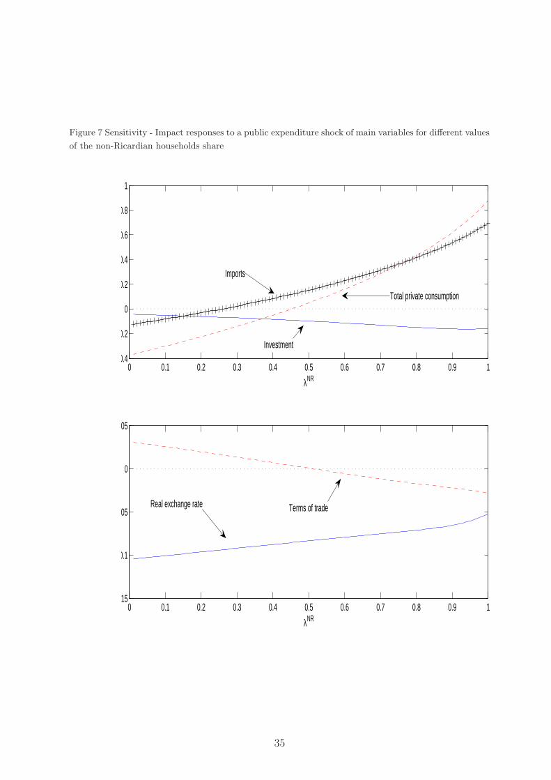
Figure 7 Sensitivity - Impact responses to a public expenditure shock of main variables for different valuesof the non-Ricardian households share
0 0.1 0.2 0.3 0.4 0.5 0.6 0.7 0.8 0.9 1−0.4
−0.2
0
0.2
0.4
0.6
0.8
1
λNR
0 0.1 0.2 0.3 0.4 0.5 0.6 0.7 0.8 0.9 1−0.15
−0.1
−0.05
0
0.05
λNR
Imports
Total private consumption
Investment
Terms of tradeReal exchange rate
35
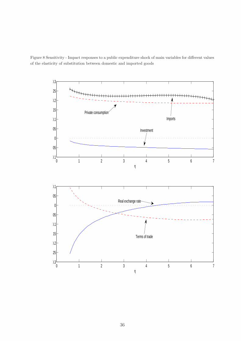
Figure 8 Sensitivity - Impact responses to a public expenditure shock of main variables for different valuesof the elasticity of substitution between domestic and imported goods
0 1 2 3 4 5 6 7−0.1
−0.05
0
0.05
0.1
0.15
0.2
0.25
0.3
η
0 1 2 3 4 5 6 7−0.3
−0.25
−0.2
−0.15
−0.1
−0.05
0
0.05
0.1
η
Terms of trade
Real exchange rate
Investment
Private consumptionImports
36
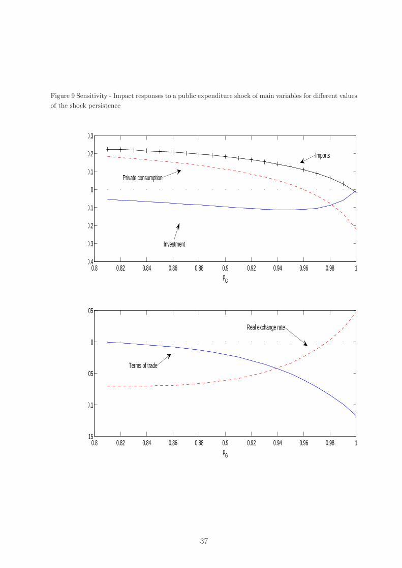
Figure 9 Sensitivity - Impact responses to a public expenditure shock of main variables for different valuesof the shock persistence
0.8 0.82 0.84 0.86 0.88 0.9 0.92 0.94 0.96 0.98 1−0.4
−0.3
−0.2
−0.1
0
0.1
0.2
0.3
ρG
0.8 0.82 0.84 0.86 0.88 0.9 0.92 0.94 0.96 0.98 1−0.15
−0.1
−0.05
0
0.05
ρG
Investment
Private consumption
Imports
Real exchange rate
Terms of trade
37