Entropy 2009, 11, 972-992; doi:10.3390/e11040972

OPEN ACCESS

entropyISSN 1099-4300

www.mdpi.com/journal/entropy

Review

Fisher Information and Semiclassical TreatmentsFlavia Pennini 1,2,⋆, Gustavo Ferri 3 and Angelo Plastino 2

1 Departamento de Fısica, Universidad Catolica del Norte, Av. Angamos 0610, Antofagasta, Chile2 Instituto de Fısica La Plata (IFLP), Facultad de Ciencias Exactas, Universidad Nacional de La Plata

(UNLP), Consejo Nacional de Investigaciones (CCT-CONICET), C.C. 727, (1900) La Plata,Argentina; E-Mail: plastino@fisica.unlp.edu.ar (A.P.)

3 Facultad de Ciencias Exactas y Naturales, Universidad Nacional de La Pampa, Uruguay 151, SantaRosa, La Pampa, Argentina; E-Mail: glferri@exactas.unlpam.edu.ar (G.F.)

⋆ Author to whom correspondence should be addressed; E-Mail: fpennini@ucn.cl.

Received: 30 October 2009 / Accepted: 27 November 2009 / Published: 3 December 2009

Abstract: We review here the difference between quantum statistical treatments andsemiclassical ones, using as the main concomitant tool a semiclassical, shift-invariantFisher information measure built up with Husimi distributions. Its semiclassical characternotwithstanding, this measure also contains abundant information of a purely quantal nature.Such a tool allows us to refine the celebrated Lieb bound for Wehrl entropies and to discoverthermodynamic-like relations that involve the degree of delocalization. Fisher-related thermaluncertainty relations are developed and the degree of purity of canonical distributions,regarded as mixed states, is connected to this Fisher measure as well.

Keywords: information theory; phase space; semiclassical information; delocalization;purity; thermal uncertainties; Fisher measures

1. Introduction

A quarter of century before Shannon, R.A. Fisher advanced a method to measure the informationcontent of continuous (rather than digital) inputs using not the binary computer codes but the statisticaldistribution of classical probability theory [1]. Already in 1980 Wootters pointed out that Fisher’sinformation measure (FIM) and quantum mechanics share a common formalism and both relateprobabilities to the squares of continuous functions [2].

Entropy 2009, 11 973

The present review draws materials from much interesting work that is reported recently anddevoted to the physical applications of Fisher’s information measure (see, for instance, [1, 3–6]).Frieden and Soffer [3] have shown that Fisher’s information measure provides one with a powerfulvariational principle—the extreme physical information—that yields most of the canonical Lagrangiansof theoretical physics [1, 3]. Additionally, FIM has been shown to provide an interesting characterizationof the “arrow of time”, alternative to the one associated with Boltzmann’s entropy [7, 8]. Thus,unravelling the multiple FIM facets and their links to physics should be of general interest. The Legendretransform structure of thermodynamics can be replicated as well, without any change, if one replaces theBoltzmann–Gibbs–Shannon entropy S by Fisher’s information measure I . In particular, I possesses theall important concavity property [5], and use of the Fisher’s measure allows for the development of athermodynamics that seems to be able to treat equilibrium and non-equilibrium situations in a mannerentirely similar to the conventional one [5]. Here, the focus of our attention will be, following [9], thethermal description of harmonic oscillator (HO).

The semiclassical approximation (SC) has had a long and distinguished history and remains today avery important weapon in the physics armory. It is indeed indispensable in many areas of scientificendeavor. Also, it facilitates, in many circumstances, an intuitive understanding of the underlyingphysics that may remain hidden in extensive numerical solutions of Schrodinger’s equation. Althoughthe SC-approach is as old as quantum mechanics itself, it remains active, as reported, for example, in [10]and [11].

Our emphasis in this review will be placed on the study of the differences between (i) statisticaltreatments of a purely quantal nature, on the one hand, and (ii) semiclassical ones, on the other. We willshow that these differences can be neatly expressed entirely in terms of a special version, to be called Iτ ,of Fisher’s information measure: the so-called shift-invariant Fisher one [1], associated to phase space.Additionally Iτ is a functional of a semiclassical distribution function, namely, the Husimi functionµ(x, p). The phase space measure Iτ will be shown to help to (1) refine the so-called Lieb-bound [12]and (2) connect this refinement with the delocalization in phase space. The latter can, of course, bevisualized as information loss. Iτ will also be related to an interesting semiclassical measure that wasearly introduced to characterize the same phenomenon: the Wehrl entropy W [12],

W = −kB⟨ ln µ ⟩µ (1)

for which Lieb established the above cited lower bound W ≥ 1, which is a manifestation of theuncertainty principle [13]. kB is the Boltzmann’s constant. Henceforth we will set kB = 1, for thesake of simplicity.

For the convenience of the reader, in the following section we describe some fundamental aspects ofthe HO canonical-ensemble description from a coherent states’ viewpoint [9], the Husimi probabilitydistribution function, and the Wehrl information measure.

Entropy 2009, 11 974

2. Background Notions

2.1. HO’s coherent states

In [9] the authors discuss quantum-mechanical phase space distributions expressed in termsof the celebrated coherent states |z⟩ of the harmonic oscillator, eigenstates of the annihilationoperator a [14, 15], i.e.,

a|z⟩ = z|z⟩ (2)

with z a complex combination of the phase space coordinates x, p

z =x

2σx

+ ip

2σp

(3)

where σx = (h/2mω)1/2, σp = (hmω/2)1/2, and σxσp = h/2.Coherent states span Hilbert’s space, constitute an over-complete basis and obey resolution of

unity [15]

∫ d2 z

π|z⟩⟨z| =

∫ dx dp

2πh|x, p⟩⟨x, p| = 1 (4)

where the differential element of area in the z−plane is d2z = dxdp/2πh and the integration is carriedout over the whole complex plane.

The coherent state |z⟩ can be expanded in terms of the states of the HO as follows

|z⟩ =∞∑

n=0

|⟨z|n⟩|2 |n⟩ (5)

where |n⟩ are eigenstates of the HO Hamiltonian whose form is H = hω [a†a + 1/2] and we have

|⟨z|n⟩|2 =|z|2n

n!e−|z|2 (6)

2.2. HO-expressions

We write down now, for future reference, well-known quantal HO-expressions for, respectively, thepartition function Z, the entropy S, the mean energy U , the mean excitation energy E, the free energyF = U − TS, and the specific heat C [16]

Z =e−βhω/2

1 − e−βhω(7)

S = βhω

eβhω − 1− ln(1 − e−βhω) (8)

U =hω

2+ E (9)

E =hω

eβhω − 1(10)

F =hω

2+ T ln(1 − e−βhω) (11)

Entropy 2009, 11 975

C =

(βhω

eβhω − 1

)2

eβhω (12)

2.3. Husimi probability distribution

In the wake of a discussion advanced in [17], we will be mainly concerned with building“Husimi–Fisher” bridges. It is well-known that the oldest and most elaborate phase space (PS)formulation of quantum mechanics is that of Wigner [18, 19]. To every quantum state a PS function(the Wigner one) can be assigned. This PS function can, regrettably enough, assume negative values sothat a probabilistic interpretation becomes questionable. Such limitation was overcome, among others,by Husimi [20]. In terms of the concomitant Husimi probability distributions, quantum mechanics canbe completely reformulated [21–24]. This phase space distribution has the form of

µ(x, p) ≡ µ(z) = ⟨z|ρ|z⟩ (13)

where ρ is the density operator of the system and |z⟩ are the coherent states (see, for instance, [25] andreferences therein). The function µ(x, p) is normalized in the fashion

∫ dx dp

2πhµ(x, p) = 1 (14)

For a thermal equilibrium case ρ = Z−1e−βH , Z = Tr(e−βH) is the partition function, β = 1/T , withT being the temperature. Specializing things for the HO of frequency ω, with eigenstates |n⟩ associatedto the eigenenergies En = hω (n + 1/2), one has

⟨z|ρ|z⟩ =1

Z

∑n

e−βH |⟨z|n⟩|2 (15)

with |⟨z|n⟩|2 given by Equation (6), and the normalized Husimi probability distribution is

µ(z) = (1 − e−βhω) e−(1−e−βhω)|z|2 (16)

2.4. Wehrl entropy

The Wehrl entropy is defined as [12]

W = −∫ dx dp

2πhµ(x, p) ln µ(x, p) (17)

where µ(x, p) is the “classical” distribution function (13) associated to the density operator ρ of thesystem. The uncertainty principle manifests itself through the inequality W ≥ 1, which was firstconjectured by Wehrl [12] and later proved by Lieb [13]. Equality holds if ρ is a coherent state. Afterintegration over all phase space, turns out to be [9]

W = 1 − ln(1 − e−βhω) (18)

Entropy 2009, 11 976

3. Fisher’s Information Measure

Let us consider a system that is specified by a physical parameter θ, while x is a real stochastic variableand fθ(x), which in turn depends on the parameter θ, is the probability density for x. An observer makesa measurement of x and estimates θ from this measurement, represented by θ = θ(x). One wonders howwell θ can be determined. Estimation theory [26] asserts that the best possible estimator θ(x), after a verylarge number of x-samples is examined, suffers a mean-square error e2 from θ that obeys a relationshipinvolving Fisher’s I , namely, Ie2 = 1, where the Fisher information measure I is of the form

I(θ) =∫

dx fθ(x)

{∂ ln fθ(x)

∂θ

}2

(19)

This “best” estimator is called the efficient estimator. Any other estimator must have a largermean-square error. The only proviso to the above result is that all estimators be unbiased, i.e., satisfy⟨θ(x)⟩ = θ. Thus, Fisher’s information measure has a lower bound, in the sense that, no matterwhat parameter of the system we choose to measure, I has to be larger or equal than the inverse ofthe mean-square error associated with the concomitant experiment. This result, I e2 ≥ 1, is referredto as the Cramer–Rao bound [1, 27]. A particular I-case is of great importance: that of translationfamilies [1, 4], i.e., distribution functions (DF) whose form does not change under θ-displacements.These DF are shift-invariant (a la Mach, no absolute origin for θ), and for them Fisher’s informationmeasure adopts the somewhat simpler appearance [1]

I =∫

dx f(x)

{∂ ln f(x)

∂x

}2

(20)

Fisher’s measure is additive [1]: If x and p are independent, variables, I(x + p) = I(x) + I(p).Notice that, for τ ≡ (x, p) (a point in phase-space), we face a shift-invariance situation. Since indefining z in terms of the variables x and p, these are scaled by their respective variances, the Fishermeasure associated to the probability distribution µ(x, p) will be of the form [4]

Iτ =∫ dx dp

2πhµ(x, p)A (21)

with

A = σ2x

[∂ ln µ(x, p)

∂x

]2

+ σ2p

[∂ ln µ(x, p)

∂p

]2

(22)

Given the µ-expression (16), Iτ becomes

Iτ = 1 − e−βhω (23)

which, immediately yields

Iτ e2|z|(β, ω) = 1; (CR bound reached) (24)

We realize at this point that the Fisher measure built up with Husimi distributions is to be bestemployed to estimate “phase space position” |z|. Further, efficient estimation is possible for alltemperatures, a rather significant result. Comparison with Equation (18) allows one now to write

Entropy 2009, 11 977

W = 1 − ln(Iτ ) ⇒ W + ln(Iτ ) = 1 (25)

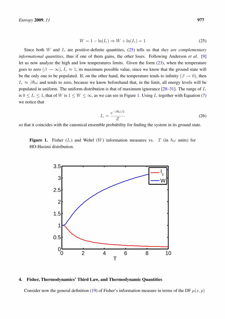
Since both W and Iτ are positive-definite quantities, (25) tells us that they are complementaryinformational quantities, thus if one of them gains, the other loses. Following Anderson et al. [9]let us now analyze the high and low temperatures limits. Given the form (23), when the temperaturegoes to zero (β → ∞), Iτ ≈ 1, its maximum possible value, since we know that the ground state willbe the only one to be populated. If, on the other hand, the temperature tends to infinity (β → 0), thenIτ ≈ βhω and tends to zero, because we know beforehand that, in the limit, all energy levels will bepopulated in uniform. The uniform distribution is that of maximum ignorance [28–31]. The range of Iτ

is 0 ≤ Iτ ≤ 1, that of W is 1 ≤ W ≤ ∞, as we can see in Figure 1. Using Iτ together with Equation (7)we notice that

Iτ =e−βhω/2

Z(26)

so that it coincides with the canonical ensemble probability for finding the system in its ground state.

Figure 1. Fisher (Iτ ) and Wehrl (W ) information measures vs. T (in hω units) forHO-Husimi distribution.

0 2 4 6 8 100

0.5

1

1.5

2

2.5

3

3.5

T

IτW

4. Fisher, Thermodynamics’ Third Law, and Thermodynamic Quantities

Consider now the general definition (19) of Fisher’s information measure in terms of the DF µ(x, p)

Entropy 2009, 11 978

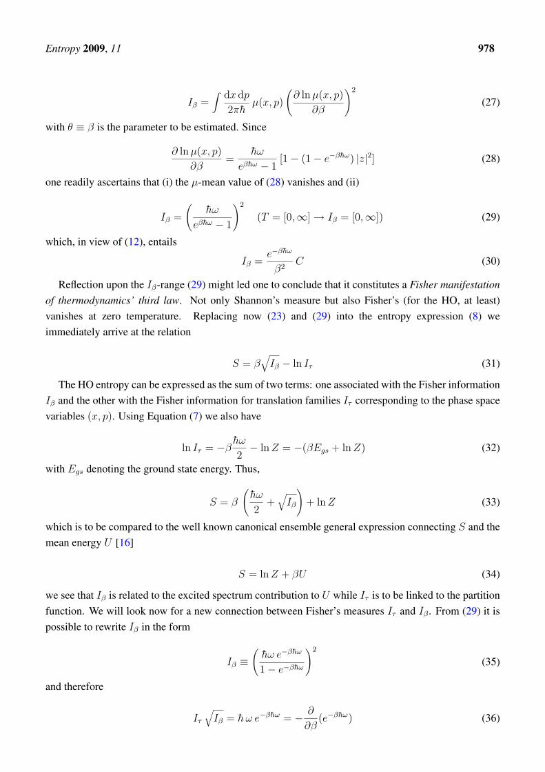
Iβ =∫ dx dp

2πhµ(x, p)

(∂ ln µ(x, p)

∂β

)2

(27)

with θ ≡ β is the parameter to be estimated. Since

∂ ln µ(x, p)

∂β=

hω

eβhω − 1[1 − (1 − e−βhω) |z|2] (28)

one readily ascertains that (i) the µ-mean value of (28) vanishes and (ii)

Iβ =

(hω

eβhω − 1

)2

(T = [0,∞] → Iβ = [0,∞]) (29)

which, in view of (12), entails

Iβ =e−βhω

β2C (30)

Reflection upon the Iβ-range (29) might led one to conclude that it constitutes a Fisher manifestationof thermodynamics’ third law. Not only Shannon’s measure but also Fisher’s (for the HO, at least)vanishes at zero temperature. Replacing now (23) and (29) into the entropy expression (8) weimmediately arrive at the relation

S = β√

Iβ − ln Iτ (31)

The HO entropy can be expressed as the sum of two terms: one associated with the Fisher informationIβ and the other with the Fisher information for translation families Iτ corresponding to the phase spacevariables (x, p). Using Equation (7) we also have

ln Iτ = −βhω

2− ln Z = −(βEgs + ln Z) (32)

with Egs denoting the ground state energy. Thus,

S = β

(hω

2+√

Iβ

)+ ln Z (33)

which is to be compared to the well known canonical ensemble general expression connecting S and themean energy U [16]

S = ln Z + βU (34)

we see that Iβ is related to the excited spectrum contribution to U while Iτ is to be linked to the partitionfunction. We will look now for a new connection between Fisher’s measures Iτ and Iβ . From (29) it ispossible to rewrite Iβ in the form

Iβ ≡(

hω e−βhω

1 − e−βhω

)2

(35)

and therefore

Iτ

√Iβ = h ω e−βhω = − ∂

∂β(e−βhω) (36)

Entropy 2009, 11 979

i.e., the product on the left hand side is the β-derivative of the Boltzmann factor (constant energy-wise)at the inverse temperature β. In other words, Iτ

√Iβ measures the β-gradient of the Boltzmann factor.

Equation (23) implies, via Equations (7) to (12), that the quantal HO expressions for the mostimportant thermodynamic quantities can be expressed in terms of the semiclassical measure Iτ . Forthis end we define the semiclassical free energy

Fsc = T ln Iτ (37)

which is the semiclassical contribution to the HO free-energy F = hω/2 + Fsc. Therefore, thethermodynamic quantities can be expressed as follows

Z =e−βhω/2

Iτ

(38)

E = hω1 − Iτ

Iτ

(39)

S = βhω1 − Iτ

Iτ

− Fsc

T(40)

C = (βhω)2 1 − Iτ

I2τ

(41)

which shows that the semiclassical, Husimi-based Iτ−information measure does contain purely quantumstatistical information. Furthermore, since from Helmholtz’ free energy F , we can derive all of the HOquantal thermodynamics [16], we see that the the HO-quantum thermostatistics is, as far as informationis considered, entirely of semiclassical nature, as it is completely expressed in terms of a semiclassicalmeasure. We emphasize thus the fact that the semiclassical quantity Iτ contains all the relevantHO-statistical quantum information.

5. HO-Semiclassical Fisher’s Measure

5.1. MaxEnt approach

All the previous results are exact. No reference whatsoever needs to be made to Jaynes’ MaximumEntropy Principle (MaxEnt) [31] up to this point. We wish now to consider a MaxEnt viewpoint. Itis shown in [14] that the HO-energy can be cast as the sum of the ground-state energy hω/2 plus theexpectation value of the HO-Hamiltonian with respect to the coherent state |z⟩, which is the sum of theground-state energy plus a semiclassical excitation energy E . One has for the semiclassical excitationHO-energy e(z) at z [14]

e(z) = ⟨z|H|z⟩ − hω/2 = hω|z|2, i.e.,Eν = hω⟨|z|2⟩ν (42)

where the last expectation value is computed using the distribution ν(z). This semiclassical excitationenergy Eµ is given, for a Husimi distribution µ, by [25]

Entropy 2009, 11 980

Eµ = ⟨e(z)⟩µ =hω

Iτ

(43)

Note now that, from Equation (16), we can conveniently recast the HO-expression for µ into theGaussian fashion

µ(z) = Iτ e−Iτ |z|2 (44)

peaked at the origin. The probability density µ of Equation (44) is clearly of the maximum entropy [31].As a consequence, it proves convenient, at this stage, to view Iτ in the following light. The

semiclassical form of the entropy S has exhaustively been studied by Wehrl. It is the (cf. 1) Shannon’sinformation measure evaluated with Husimi distributions [12]. Assume we know a priori the valueEν = hω⟨|z|2⟩ν . We wish to determine the distribution ν(z) that maximizes the Wehrl entropy under thisEν−value constraint. Accordingly, the MaxEnt distribution will be [31]

ν(z) = e−λoe−η E(z) (45)

with λo the normalization Lagrange multiplier and η the one associated to Eν . According to MaxEnttenets we have [31]

λo = λo(η) = ln∫ d2z

πe−η hω|z|2 = − ln (η hω) (46)

Now, the η−multiplier is determined by the relation [31]

− Eν =∂λo

∂η= −1

η(47)

If we choose the Fisher-Husimi constraint given by Equation (43), this results in η = Iτ/hω and fromEquation (46) we get λo = − ln Iτ , i.e., e−λo = Iτ , and we consequently arrive to the desired outcome

ν(z) = Iτ e−Iτ |z|2 ≡ µ(z) (48)

We have thus shown that the HO-Husimi distributions are MaxEnt-ones with the semiclassicalexcitation energy (43) as a constraint. It is clear from Equation (48) that Iτ plays there the role ofan “inverse temperature”.

The preceding argument suggests that we are tacitly envisioning the existence of a quantity TW (theinverse of η) associated to the Wehrl measure that we here extend to extreme. This Wehrl temperatureTW governs the width of our Gaussian Husimi distribution. On account of

µ(z) = Iτ e−(Iτ /hω) hω|z|2 = Iτ e−Eµ/TW (49)

which entails

TW =hω

Iτ

(50)

and it is easy to see from the range of Iτ that the range of values of TW is then hω ≤ TW ≤ ∞. Due tothe semiclassical nature of both W and µ, TW has a lower bound greater than zero.

Entropy 2009, 11 981

5.2. Delocalization

The two quantities W and Iτ have been shown to be related, for the HO, according to Equation (25).Since the Wehrl temperature TW yields the width of our Gaussian Husimi distribution, we can conceiveof introducing a “delocalization factor” D

D =TW

hω(51)

The above definition leads to the relation

W = 1 + ln TW − ln hω = 1 + ln D (52)

As stressed above, W has been constructed as a delocalization measure [12]. The precedingconsiderations clearly motivate one to regard the Fisher measure built up with Husimi distributionsas a “localization estimator” in phase space. The HO-Gaussian expression for µ (44) illuminates thefact that the Fisher measure controls both the height and the spread (which is ∼ [2Iτ ]

−1). Obviously,spread is here a “phase-space delocalization indicator”. This fact is reflected by the quantity D

introduced above.Thus, an original physical interpretation of Fisher’s measure emerges: localization control. The

inverse of the Fisher measure, D, turns out to be a delocalization-indicator. Differentiating Fisher’smeasure (23) with respect T , notice also that

dIτ

dT= − hω

T 2e−βhω (53)

so that Fisher’s information decreases exponentially as the temperature grows. Our Gaussian distributionloses phase-space “localization” as energy and/or temperature are injected into our system, as reflectedvia TW or D. Notice that (52) complements the Lieb bound W ≥ 1. It tells us by just how muchW exceeds unity. We see that it does it by virtue of delocalization effects. Moreover, this fact canbe expressed using the shift-invariant Fisher measure. We will now show that D is proportional to thesystem’s energy fluctuations.

5.3. Second moment of the Husimi distribution

The second moment of the Husimi distribution µ(z) is an important measure to ascertain the “degreeof complexity” of a quantum state (see below). It is a measure of the delocalization-degree of the Husimidistribution in phase space (see Reference [32] for details and discussions). It is defined as

M2 =∫ d2z

πµ2(z) (54)

that, after explicit evaluation of M2 from Equation (44) reads

M2 =Iτ

2(55)

Using now (52) we conclude that

M2(D) =1

2 D(56)

Entropy 2009, 11 982

Thus, our energy-fluctuations turn out to be

∆µe =hω

Iτ

= hω D (57)

with (∆µe)2 = (E2)µ − E2

µ. As a consequence, we get

D =∆µe

hω(58)

An important result is thus obtained: the delocalization factor D represents energy-fluctuationsexpressed in hω−terms. Delocalization is clearly seen to be the counterpart of energy fluctuations.

6. Thermodynamics-Like Relations

Let us now go back to Equation (37) and revisit the entropic expression. It is immediately realizedthat we can recast the entropy S in terms of the quantal mean excitation energy E and the delocalizationfactor D as

E

T= S − ln D (59)

i.e., if one injects into the system some excitation energy E, expressed in “natural” T units, it isapportioned partly as heat dissipation via S and partly via delocalization. More precisely, the partof this energy not dissipated is that employed to delocalize the system in phase space. Now, sinceW = 1 − ln Iτ = 1 + ln D, the above equation can be recast in alternative forms, as

S =E

T+ ln D =

E

T− ln Iτ ; or (60)

W = 1 + S − E

T(61)

implying

W − S 7→ 0 for T 7→ ∞ (62)

which is a physically sensible result and

W − S 7→ 1 for T 7→ 0 (63)

as it should, since S = 0 at T = 0 (third law of thermodynamics), while W attains there its Lieb’s lowerbound of unity.

One finds in Equation (60) some degree of resemblance to thermodynamics’s first law. To reassureourselves on this respect, we slightly changed our underlying canonical probabilities µ, multiplying itby a factor δF = random number/100. Specifically, we generated random numbers according to thenormal distribution and divided them by 100 to obtain the above factors δF . This process leads to new“perturbed” probabilities P = µ+δµ, conveniently normalized. With them we evaluate the concomitantchanges dS, dE (we do this 50 times, with different random numbers in each instance). We were thenable to numerically verify that the difference dS − βdE ∼ 0. The concomitant results are plotted in

Entropy 2009, 11 983

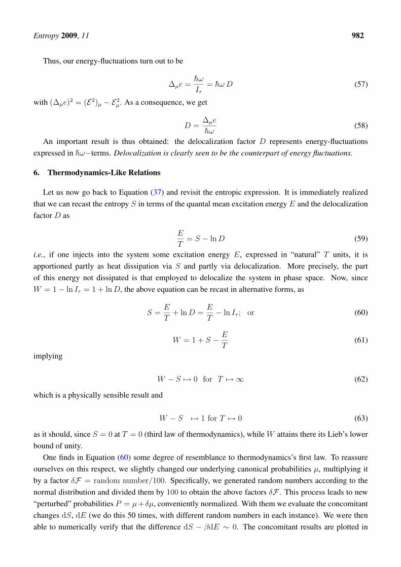
Figure 2) Since, as stated, numerically dS = (1/T ) dE, this entails, from Equation (60), dIτ/Iτ ≃ 0.The physical connotations are as follows: if the only modification effected is that of a change δµ [16] inthe canonical distribution µ, this implies that the system undergoes a heat transfer process [16] for whichthermodynamics’ first law implies dU = TdS. This is numerically confirmed in the plots of Figure 2.The null contribution of ln Iτ to this process suggests that delocalization (not a thermodynamic effect,but a dynamic one) can be regarded as behaving (thermodynamically) like a kind of “work”.

Figure 2. Numerical computation results for the HO: changes dU and dIτ vs. dS thatensue after randomly generating variations δpi in the underlying microscopic canonicalprobabilities pi.

−0.015 −0.01 −0.005 0 0.005 0.01 0.015−0.015

−0.01

−0.005

0

0.005

0.01

0.015

dS

dU

, dI τ

T/hν = 1dUdIτ

Now, since (a) Iτ = 1 − e−βhω, and (b) the mean energy of excitation is E = hω/(exp (βhω) − 1),one also finds, for the quantum-semiclassical difference (QsCD) S − W the result

W − S = 1 − Iτ−1Iτ

ln(1 − Iτ ) = F1(Iτ ) (64)

Moreover, since 0 ≤ F1(Iτ ) ≤ 1, we see that, always, W ≥ S, as expected, since the semiclassicaltreatment contains less information than the quantal one. Note that the QsCD can be expressedexclusively in Fisher’s information terms. This is, the quantum-semiclassical entropic difference S −W

may be given in Iτ−terms only. Figure (3) depicts S, βE, and ln D vs. the dimensionless quantityt = T/hω. Accordingly, entropy is apportioned in such a way that

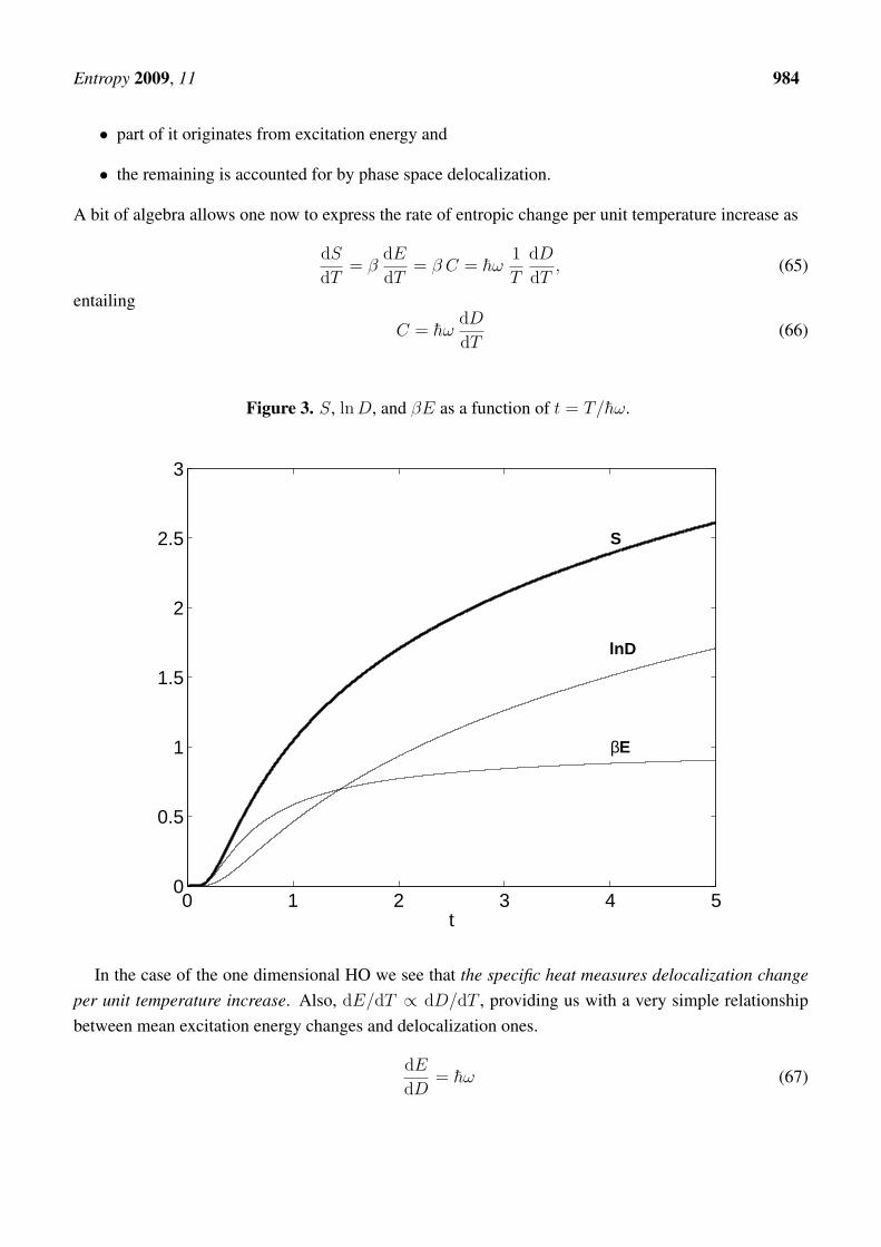
Entropy 2009, 11 984

• part of it originates from excitation energy and

• the remaining is accounted for by phase space delocalization.

A bit of algebra allows one now to express the rate of entropic change per unit temperature increase as

dS

dT= β

dE

dT= β C = hω

1

T

dD

dT, (65)

entailing

C = hωdD

dT(66)

Figure 3. S, ln D, and βE as a function of t = T/hω.

0 1 2 3 4 50

0.5

1

1.5

2

2.5

3

βE

lnD

S

t

In the case of the one dimensional HO we see that the specific heat measures delocalization changeper unit temperature increase. Also, dE/dT ∝ dD/dT , providing us with a very simple relationshipbetween mean excitation energy changes and delocalization ones.

dE

dD= hω (67)

Entropy 2009, 11 985

7. On Thermal Uncertainties

Additional considerations are in order with regards to thermal uncertainties, that express the effectof temperature on Heisenberg’s celebrated relations (see, for instance [6, 33–35]). We use now a resultobtained in [9] (Equation (3.12)), where the authors cast Wehrl’s information measure in terms of thecoordinates’ variances ∆µx and ∆µp, obtaining

W = ln{

e

h∆µx ∆µp

}(68)

In the present context, the relation W = 1 − ln Iτ allows us to conclude that [17]

Iτ ∆µx ∆µp = h (69)

which can be regarded as a “Fisher uncertainty principle” and adds still another meaning to Iτ : since,necessarily, ∆µx ∆µp ≥ h/2, it is clear that Iτ/2 is the “correcting factor” that permits one to reach theuncertainty’s lower bound h/2, a rather interesting result.

Phase space “localization” is possible, with Husimi distributions, only up to h [14]. This is to becompared to the uncertainties evaluated in a purely quantal fashion, without using Husimi distributions,and in particular with a previous result in [17]. With the virial theorem [16] one can easily ascertainin [17] that

∆x ∆p =h

2

eβhω + 1

eβhω − 1(70)

together with (69) yields

∆µx ∆µp =2 ∆x ∆p

1 + e−βhω(71)

Thus We see that, as β → ∞, ∆µ ≡ ∆µx ∆µp is twice the minimum quantum value for ∆x∆p,and ∆µ → h, the “minimal” phase-space cell. The quantum and semiclassical results do coincide atvery high temperature though. Indeed, one readily verifies [17] that Heisenberg’s uncertainty relation,as a function of both frequency and temperature, is governed by a thermal “uncertainty function” F thatacquires the aspect

F (β, ω) = ∆x ∆p =1

2

[∆µ +

E

ω

](72)

Coming back to results derivable within the present context, we realize here that F can be recast as

F (β, ω) =1

2

[h D +

E

ω

](73)

so that, for T varying in [0,∞], the range of possible ∆x ∆p-values is [h/2,∞]. Equation (73)is a “Heisenberg–Fisher” thermal uncertainty relation (for a discussion of this concept see, forinstance, [6, 33, 34]).

F (β, ω) grows with both E and D. The usual result h/2 is attained for minimum D and zero excitationenergy. As for dF/dT , one is able to set F ≡ F (E, D), since 2dF = hdD + ω−1dE. Remarkably

Entropy 2009, 11 986

enough, the two contributions to dF/dT are easily seen to be equal and dF/dT → (1/ω) for T → ∞.One can also write (

∂F

∂D

)E

=h

2;

(∂F

∂E

)D

=1

2ω(74)

providing us with a thermodynamic “costume” for the uncertainty function F that sheds some new lightonto the meaning of both h and ω. In particular, we see that h/2 is the derivative of the uncertaintyfunction F with respect to the delocalization factor D. Increases dF of the thermal uncertainty functionF are of two types

• from the excitation energy, that supplies a C/ω contribution and

• from the delocalization factor D.

8. Degrees of Purity Relations

8.1. Semiclassical purity

The quantal concept of degree of purity of a general density operator ρ is expressed via Tr ρ2 [36, 37].Its inverse, the so-called participation ratio

R =1

Tr ρ2(75)

is particularly convenient for calculations [38]. It varies from unity for pure states to N for totally mixedstates [38]. It may be interpreted as the effective number of pure states that enter a quantum mixture.Here we will consider the “degree of purity” dµ of a semiclassical distribution, given by

dµ =∫ d2z

πµ2(z) ≤ 1 (76)

Clearly, dµ coincides with the second moment of the Husimi distribution (44) given by Equation (54),i.e.,

dµ = M2 =Iτ

2(77)

Using now (52) we relate the semiclassical degree of purity to the delocalization factor and to theWehrl temperature TW

dµ =1

2 D=

TW

2hω(78)

and also to our semiclassical energy-fluctuations (57)

dµ =hω

2∆µe(79)

Since hω ≤ TW ≤ ∞, the “best” purity attainable at the semiclassical level equals one-half.

Entropy 2009, 11 987

8.2. Quantal purity

For the quantum mixed HO-state ρ = e−βH/Z, where H is the Hamiltonian of the harmonic oscillatorand the partition function Z is given by Equation (7) [16], we have a degree of purity dρ given by (seethe detailed study by Dodonov [35])

dρ =e−βhω

Z2

∞∑n=0

e−2βhωn (80)

leading to

dρ = tanh(βhω/2) (81)

where 0 ≤ dρ ≤ 1. Thus, Heisenberg’ uncertainty relation can be cast in the fashion

∆x ∆p =h

2coth(βhω/2) (82)

where ∆x and ∆p are the quantum variances for the canonically conjugated observables x and p [35]

∆x ∆p =h

2

1

dρ

(83)

which is to be compared to the semiclassical result that was derived above (cf. 71).We relate now the degree of purity of our thermal state with various physical quantities both in its

quantal and semiclassical versions. Using Equations (71) and (77) we get

dµ =Iτ

2= (1 − dµ) dρ (84)

which leads to

dρ =dµ

1 − dµ

=Iτ

2 − Iτ

dµ =dρ

1 + dρ

(85)

such as clearly shows that (i) dµ ≤ dρ, and (ii) for a pure state, again, its semiclassical counterpart has adegree of purity equal 1/2.

Additionally, on account of Equation (69), on the one hand, and since the semiclassical degree ofpurity reads dµ = Iτ/2, on the other one, we are led to an uncertainty relation for mixed states in termsof dµ, namely,

∆µx ∆µp =h

2

1

dµ

(86)

that tells us just how uncertainty grows as participation ratio R = 1/dµ augments. Equation (86) isof semiclassical origin, which makes it a bit different from the one that results form a purely quantaltreatment (see [35], Equation (4)). Moreover, notice how information concerning the purely quantalnotion of purity dρ is already contained in the semiclassical measure Iτ .

Entropy 2009, 11 988

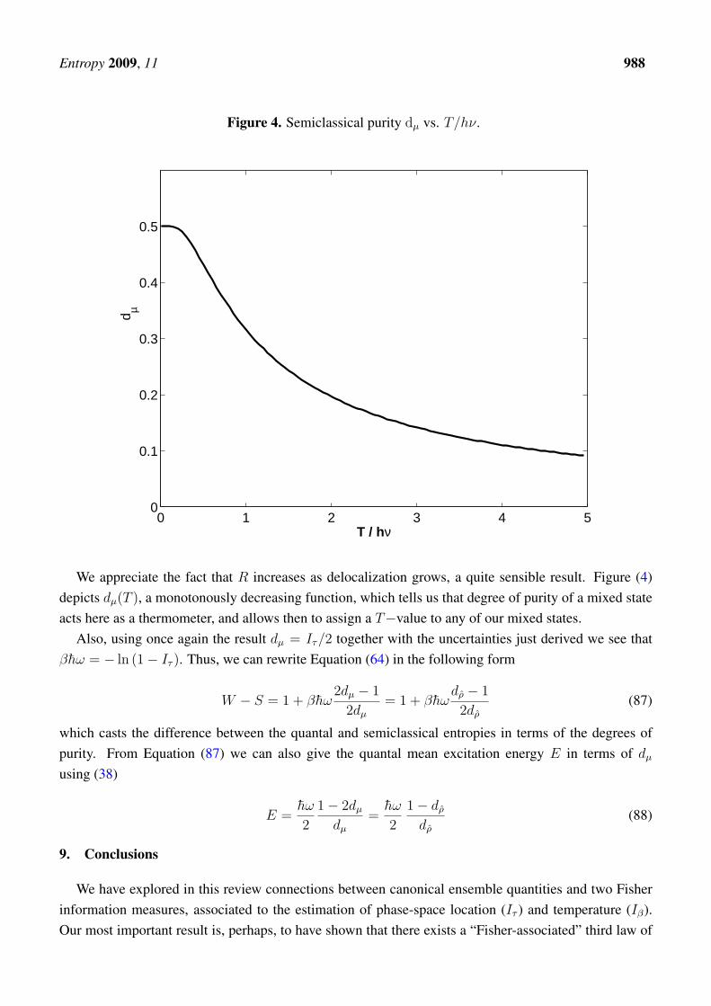
Figure 4. Semiclassical purity dµ vs. T/hν.

0 1 2 3 4 50

0.1

0.2

0.3

0.4

0.5

T / hν

d µ

We appreciate the fact that R increases as delocalization grows, a quite sensible result. Figure (4)depicts dµ(T ), a monotonously decreasing function, which tells us that degree of purity of a mixed stateacts here as a thermometer, and allows then to assign a T−value to any of our mixed states.

Also, using once again the result dµ = Iτ/2 together with the uncertainties just derived we see thatβhω = − ln (1 − Iτ ). Thus, we can rewrite Equation (64) in the following form

W − S = 1 + βhω2dµ − 1

2dµ

= 1 + βhωdρ − 1

2dρ

(87)

which casts the difference between the quantal and semiclassical entropies in terms of the degrees ofpurity. From Equation (87) we can also give the quantal mean excitation energy E in terms of dµ

using (38)

E =hω

2

1 − 2dµ

dµ

=hω

2

1 − dρ

dρ

(88)

9. Conclusions

We have explored in this review connections between canonical ensemble quantities and two Fisherinformation measures, associated to the estimation of phase-space location (Iτ ) and temperature (Iβ).Our most important result is, perhaps, to have shown that there exists a “Fisher-associated” third law of

Entropy 2009, 11 989

thermodynamics (at least for the HO). From a pure information-theoretic viewpoint, we have, obtainedsignificant results, namely,

1. a connection between Wehrl’s entropy and Iτ (cf. Equation (25)),

2. an interpretation of Iτ as the HO’s ground state occupation probability (cf. Equation (26)),

3. an interpretation of Iβ proportional to the HO’s specific heat (cf. Equation (30)),

4. the possibility of expressing the HO’s entropy as a sum of two terms, one for each of the aboveFIM realizations (cf. Equation (31)),

5. a new form of Heisenberg’s uncertainty relations in Fisher terms (cf. Equation (73)),

6. that efficient |z|-estimation can be achieved with Iτ at all temperatures, as the minimumCramer–Rao value is always reached (cf. Equation (24)).

Our statistical semiclassical treatment yielded, we believe, some new interesting physics that weproceed to summarize. We have, for the HO,

1. established that the semiclassical Fisher measure Iτ contains all relevant statistical quantuminformation,

2. shown that the Husimi distributions are MaxEnt ones, with the semiclassical excitation energy Eas the only constraint,

3. complemented the Lieb bound on the Wehrl entropy using Iτ ,

4. observed in detailed fashion how delocalization becomes the counterpart of energy fluctuations,

5. written down the difference W−S between the semiclassical and quantal entropy also in Iτ−terms,

6. provided a relation between energy excitation and degree of delocalization,

7. shown that the derivative of twice the uncertainty function F (βω) = ∆x∆p with respect to I−1τ is

the Planck constant h,

8. established a semiclassical uncertainty relation in terms of the semiclassical purity dµ, and

9. expressed both dµ and the quantal degree of purity in terms of Iτ .

These results are, of course, restricted to the harmonic oscillator. However, this is such an importantsystem that HO insights usually have a wide impact, as the HO constitutes much more than a mereexample. Nowadays it is of particular interest for the dynamics of bosonic or fermionic atoms containedin magnetic traps [39–41] as well as for any system that exhibits an equidistant level spacing in thevicinity of the ground state, like nuclei or Luttinger liquids. The treatment of Hamiltonians includinganharmonic terms is the next logical step. We are currently undertaking such a task. To this endanalytical considerations do not suffice, and numerical methods are required. The ensuing results will bepublished elsewhere.

Entropy 2009, 11 990

Acknowledgements

F. Pennini is grateful for the financial support by FONDECYT, grant 1080487.

References and Notes

1. Frieden, B.R. Science from Fisher Information, 2nd ed.; Cambridge University Press: Cambridge,UK, 2004.

2. Wootters, W.K. The acquisition of information from quantum measurements. PhD Dissertation,University of Texas, Austin, TX, USA, 1980.

3. Frieden, B.R.; Soffer, B.H. Lagrangians of physics and the game of Fisher-information transfer.Phys. Rev. E 1995, 52, 2274-2286.

4. Pennini, F.; Plastino, A.R.; Plastino, A. Renyi entropies and Fisher informations as measures ofnonextensivity in a Tsallis setting. Physica A 1998, 258, 446-457.

5. Frieden, B.R.; Plastino, A.; Plastino, A.R.; Soffer, H. Fisher-based thermodynamics: Its Legendretransformations and concavity properties. Phys. Rev. E 1999, 60, 48-53.

6. Pennini, F.; Plastino, A.; Plastino, A.R.; Casas, M. How fundamental is the character of thermaluncertainty relations? Phys. Lett. A 2002, 302, 156-162.

7. Plastino, A.R.; Plastino, A. Symmetries of the Fokker-Planck equation and the Fisher-Friedenarrow of time. Phys. Rev. E 1996, 54, 4423-4426.

8. Plastino, A.; Plastino, A.R.; Miller, H.G. On the relationship between the Fisher-Frieden-Sofferarrow of time, and the behaviour of the Boltzmann and Kullback entropies. Phys. Lett. A 1997,235, 129-134.

9. Anderson, A.; Halliwell, J.J. Information-theoretic measure of uncertainty due to quantum andthermal fluctuations. Phys. Rev. D 1993, 48, 2753-2765.

10. Dimassi, M.; Sjoestrand, J. Spectral Asymptotics in the Semiclassical Limit; Cambridge UnivesityPress: Cambridge, UK, 1999.

11. Brack, M.; Bhaduri, R.K. Semiclassical Physics; Addison-Wesley: Boston, MA, USA, 1997.12. Wehrl, A. On the relation between classical and quantum entropy. Rep. Math. Phys. 1979, 16,

353-358.13. Lieb, E.H. Proof of an entropy conjecture of wehrl. Commun. Math. Phys. 1978, 62, 35-41.14. Schnack, J. Thermodynamics of the harmonic oscillator using coherent states. Europhys. Lett.

1999, 45, 647-652.15. Klauder, J.R.; Skagerstam, B.S. Coherent States; World Scientific: Singapore, 1985.16. Pathria, R.K. Statistical Mechanics; Pergamon Press: Exeter, UK, 1993.17. Pennini, F.; Plastino, A. Heisenberg–Fisher thermal uncertainty measure. Phys. Rev. E 2004, 69,

057101:1-57101:4.18. Wigner, E.P. On the quantum correction for thermodynamic equilibrium. Phys. Rev. 1932, 40,

749-759.19. Wlodarz, J.J. Entropy and wigner distribution functions revisited. Int. J. Theor. Phys. 2003, 42,

1075-1084.

Entropy 2009, 11 991

20. Husimi, K. Some formal properties of the density matrix. Proc. Phys. Math. Soc. JPN 1940, 22,264-283.

21. O’ Connel, R.F.; Wigner, E.P. Some properties of a non-negative quantum-mechanical distributionfunction. Phys. Lett. A 1981, 85, 121-126.

22. Mizrahi, S.S. Quantum mechanics in the Gaussian wave-packet phase space representation.Physica A 1984, 127, 241-264.

23. Mizrahi, S.S. Quantum mechanics in the Gaussian wave-packet phase space representation II:Dynamics. Physica A 1986, 135, 237-250.

24. Mizrahi, S.S. Quantum mechanics in the gaussian wave-packet phase space representation III:From phase space probability functions to wave-functions. Physica A 1988, 150, 541-554.

25. Pennini, F.; Plastino, A. Escort Husimi distributions, Fisher information and nonextensivity. Phys.Lett. A 2004, 326, 20-26.

26. Cramer, H. Mathematical Methods of Statistics; Princeton University Press: Princeton, NJ, USA,1946.

27. Rao, C.R. Information and accuracy attainable in the estimation of statistical parameters. Bull.Calcutta Math. Soc. 1945, 37, 81-91.

28. Jaynes, E.T. Information theory and statistical mechanics I. Phys. Rev. 1957, 106, 620-630.29. Jaynes, E.T. Information theory and statistical mechanics II. Phys. Rev. 1957, 108, 171-190.30. Jaynes, E.T. Papers on Probability, Statistics and Statistical Physics; Rosenkrantz, R.D., Ed.;

Kluwer Academic Publishers: Norwell, MA, USA, 1987.31. Katz, A. Principles of Statistical Mechanics: The Information Theory Approach: Freeman and Co.:

San Francisco, CA, USA, 1967.32. Sugita, A.; Aiba, H. Second moment of the Husimi distribution as a measure of complexity of

quantum states. Phys. Rev. E 2002, 65, 36205:1-36205:10.33. Mandelbrot, B. The role of sufficiency and of estimation in thermodynamics. Ann. Math. Stat.

1962, 33, 1021-1038.34. Pennini, F.; Plastino, A. Power-law distributions and Fisher’s information measure. Physica A

2004, 334, 132-138.35. Dodonov, V.V. Purity- and entropy-bounded uncertainty relations for mixed quantum states. J. Opt.

B Quantum Semiclass. Opt. 2002, 4, S98-S108.36. Munro, W.J.; James, D.F.V.; White, A.G.; Kwiat, P.G. Maximizing the entanglement of two mixed

qubits. Phys. Rev. A 2003, 64, 30302:1-30302:4.37. Fano, U. Description of states in quantum mechanics by density matrix and pperator techniques.

Rev. Mod. Phys. 1957, 29, 74-93.38. Batle, J.; Plastino, A.R.; Casas, M.; Plastino, A. Conditional q-entropies and quantum separability:

A numerical exploration. J. Phys. A Math. Gen. 2002, 35, 10311-11324.39. Anderson, M.H.; Ensher, J.R.; Matthews, M.R.; Wieman, C.E.; Cornell, E.A. Observation of

bose-einstein condensation in a dilute atomic vapor. Science 1995, 269, 198-201.40. Davis, K.B.; Mewes, M.-O.; Andrews, M.R.; van Druten, N.J.; Durfee, D.S.; Kurn, D.M.; Ketterle,

W. Bose-einstein condensation in a gas of sodium atoms. Phys. Rev. Lett. 1995, 75, 3969-3973.

Entropy 2009, 11 992

41. Bradley, C.C.; Sackett, C.A.; Hulet, R.G. Bose-einstein condensation of lithium: Observation oflimited condensate number. Phys. Rev. Lett. 1997, 78, 985-989.

42. Curilef, S.; Pennini, F.; Plastino, A.; Ferri, G.L. Fisher information, delocalization and thesemiclassical description of molecular rotation. J. Phys. A Math. Theor. 2007, 40, 5127-5140.

c⃝ 2009 by the authors; licensee Molecular Diversity Preservation International, Basel, Switzerland.This article is an open-access article distributed under the terms and conditions of the Creative CommonsAttribution license (http://creativecommons.org/licenses/by/3.0/).