Semiclassical and Adiabatic Approximationin Quantum Mechanics

V.L. Pokrovsky

Contents

I. Introduction 1A. Historical remarks. 1

II. Semiclassical approximation 2A. De�nition and criterion of validity 2B. One-dimensional case: Intuitive consideration. 2C. One-dimensional case: Formal derivation 2D. Quantum penetration into classically forbidden region 3E. Passing the turning point 3F. The Bohr�s quantization rule 5G. An excursion to classical mechanics 6H. The under-barrier tunneling 7I. Decay of a metastable state 7J. The resonance tunnelling and the Ramsauer e¤ect 8K. The overbarrier re�ection. 9L. Splitting of levels in a symmetric double well. 11M. Semiclassical approximation for the radial wave

equation 12

III. Semiclassical approximation in 3 dimensions 12A. Hamilton-Jacobi equation 12B. The caustics and tubes of trajectories 14C. Bohr�s quantization in 3 dimensions. Deterministic

chaos in classical and quantum mechanics 15

IV. Adiabatic approximation 16A. De�nition and main problems 16B. Transitions at avoided two-level crossing

(Landau-Zener problem) 17C. Berry�s phase, Berry�s connection 19

1. De�nition of the geometrical phase 192. Gauge transformations 203. Invariant Berry�s phase 21

References 22

I. INTRODUCTION

In this notes we consider the semiclassical approxima-tion (SA) in Quantum Mechanics. Though this approx-imation is presented in the most of textbooks on Quan-tum Mechanics, there is hardly any other topic whicharises so many confusions. Often the authors know thecorrect result, but the derivation is impossible to under-stand. Even such brilliant textbooks as Landau and Lif-shitz (1) and by Merzbacher (2) did not avoid substantialomissions and inaccuracies. Some special questions, es-pecially related to the multi-dimensional version of theSA can be found in the book by Zeldovich and Perelo-mov (3). There exists a waste mathematical literatureon the subject from which I can recommend the bookby Maslov and Fedoryuk (4). Unfortunately this litera-ture is not very useful for physicists because of excessivemathematical rigor and abundance of notations.

On the other hand, the SA plays a special role inQuantum Mechanics since it demonstrates in a simpleanalytical form basic phenomena: energy quantization,quantum tunnelling, resonance scattering and tunnelling,overbarrier re�ection, Aharonov-Bohm e¤ect. Its time-dependent modi�cation, adiabatic approximation, allowsto solve many problems in atomic and molecular physicsand leads to mportant notions such as the Berry�s phase.L. Landau and C. Zener proposed a simple theory of tran-sitions at avoided two-level crossing, which plays funda-mental role in theory of chemical reactions, atomic scat-tering, interaction of atoms with the resonant laser �eld,dynamics of disordered systems, quantum computing etc.Besides that, the SA gives the energy spectrum with a

reasonable accuracy even in the range where its validityis not guaranteed. It allows to calcualate energy densityfor many systems including deterministic systems withchaotic spectrum and random systems. It is worthwhileto remind that the initial form of quantum theory of theatom by N. Bohr can be treated just as semiclassical ap-proximation from the point of view of modern QuantumMechanics.In these notes we use the following system of refer-

ences: equations inside a subsection are enumerated bythe letter of the subsection and their numbers. An equa-tion from another section is referred additionally by thesection number.

A. Historical remarks.

Semiclassical approximation in Quantum Mechanicswas formulated independently by G. Wentzel (Germany),H. Kramers (Holland) and L. Brilloin (France) in 1927and was coined as the WKB approximation. In manybooks and articles this abbreviation is appended by theletter J from the left, honoring an English mathematicianH. Je¤rys, who developed the approximation in 20th cen-tury. However, essential ideas of this approximation wereformulated in the beginning of the XIX century by thefamous mathematicians Cauchy and Bessel. Very im-portant features of the SA were discovered by Stokes,who studied properties of the so-called Airy equation inthe middle of the 19th century. The SA was appliedto physical acoustic by Lord Rayleigh in the end of theXIX century. H. Poincare has formulated the SA as aseries expansion and Borel proposed a general methodof summation for these divergent series in the beginningof the 20th century. Thus, the question already had along history when Quantum Mechanics was formulated

2

in 1925-1926.The semiclassical approximation was developed by

many people afterwards. The names of G.Gamov, H.Furry, E. Kemble, V. Fock, L. Landau, C. Zener, V.Maslov, I. Keller, M. Berry, M. Kruskal, M. Gutzwillermust be mentioned. The semiclassical approximation isstill not exhausted. New essential results were obtainedquite recently.

II. SEMICLASSICAL APPROXIMATION

A. De�nition and criterion of validity

This is approximation of a short de Broglie wave-length�. Namely, the necessary condition for this approxima-tion reads: � << L, where L is a characteristic lengthfor variation of potential V (r). In classical mechanics itis possible to determine the dependence of the momen-tum modulus p on coordinate r at a �xed value of energyE: p(r) =

p2m(E � V (r)). The local value of the de

Broglie wavelength is � (r) =2�~=p(r). In terms of thelocal wavelength the explicit validity criterion for semi-classical approximation reads:

j r� j= � j rV jj(E � V (r))j << 1 (A1)

It means that the variation of the potential energy at thewavelength is small in comparison to the kinetic energy.It is clear from the inequality (1) that the semiclassi-cal approximation regularly fails near classical turningpoints at which E = V (r). The semiclassical approxi-mation (SA) often allows to study qualitatively and evenquantitatively e¤ects, otherwise hopeless for an analyti-cal solution.

B. One-dimensional case: Intuitive consideration.

We start with the simple case of one dimension. Aswe discussed in subsection A, the wavelength � or mo-mentum p varies slowly in space. If it does not change atall, the wave-function for a wave propagating to the right(left) would be �(x) = Ce�ipx=~. Since p(x) changesslowly, this dependence is valid only locally. It meansthat on passing a distance �x, small in comparison to L,but possibly larger than �, the phase of the wave-functionis changed by �p(x)�x=~. Summing up many such con-tributions, we arrive at wave-functions of the type:

� = C(x) exp(�iZ x

x0

p(x0)dx0=~) (B1)

It can be shown that, at varying p(x), the former constantC(x) becomes also a slowly varying function of x. Indeedfor the wave-functions B1 the current j reads:

j� =~2mi

� ��

d �dx

� �d ��dx

�= �p(x)

mj C2(x) j

(B2)For stationary Schrödinger equation (SE) the current isconstant. Therefore C(x) = C=

pp(x). Thus, we have

found two independent solutions corresponding to prop-agating waves as

�(x) =1pp(x)

e�iR xx0pdx0=~

; p =p2m(E � V (x))

(B3)A general solution of the SE must be an arbitrary lin-ear combination of the two independent solutions (B1).Looking at them, we see that they formally diverge atclassical turning points, at which V (x) = E and p(x) = 0.Note, that they are regular points of the SE and the solu-tions have no singularity at them. It is the approximationthat becomes invalid near them.Sometimes we will use the wave-vector k(x) = p(x)=~

to simplify formulae:

�(x) =1pk(x)

e�i

xRx0

kdx

(B4)

C. One-dimensional case: Formal derivation

It is useful to derive the asymptotic equation (B3) for-mally to estimate their precision. Let us right down theSchrödinger equation (SE) in the form:

~2d2

dx2+ p2(x) = 0; p2(x) = 2m(E � V (x)) (C1)

We introduce a new sought function S(x) by a followingsubstitution: (x) = eiS=~. Then equation (C1) reads:

�dS

dx

�2� i~d

2S

dx2= p2(x) (C2)

This nonlinear di¤erential equation is equivalent to thelinear SE (C1). We solve it approximately by expandingS into a formal power series in ~:

S = S0 + ~S1 + ~2S2 + ::: (C3)

Plugging (C3) into (C2) and keeping only terms indepen-dent on ~, we �nd:

�dS0dx

�2= p2(x);

dS0dx

= �p(x) (C4)

or:

3

S0 = �xZ

x0

pdx (C5)

This is the classical action for one-dimensional motion.Retaining in the next approximation terms linear in ~,we �nd:

2dS0dx

dS1dx

= id2S0dx2

(C6)

or:

S1 =i

2ln p(x) + c (C7)

Substituting (C5) and (C7) into = eiS(x)=~, we arriveagain at the solution (B3). To estimate a correction toit, we �nd S2. In the same way:

dS2dx

=

"��dS1dx

�2+ i

d2S1dx2

#��2dS0dx

�The correction to action is:

~S2 = ~Z x

x0

3p02 � 2pp008p3

dx = o

�~pL

�= o

��

L

�(We accepted that each derivative contributes 1=L, theintegration contributes L). Thus, the second correctionis small.

D. Quantum penetration into classically forbidden region

A classical particle can not penetrate into the regionin which V (x) > 0 since it violates the energy conserva-tion. The quantum particle can be found in classicallyforbidden range because the coordinate is not compatiblewith the energy. When coordinate is �xed the energy isuncertain. The e¤ect of penetration is incorporated inthe semiclassical approximation. Indeed at V (x) > Ethe square of momentum p2(x) becomes imaginary. Butstill the two solutions (B3) are valid. One of them expo-nentially decreases in the classically forbidden region, forexample:

� =1pj p j

exp

0@� xZx0

j p j dx0=~

1A (D1)

This solution corresponds to the quantum penetration ofa particle. Another solution + grows exponentially withx growing. Often it can be rejected from a physical point

x0

x

V(x)

Classically forbiddenClassically allowed

E

FIG. 1 Quantum penetration into classically forbidden area.

of view. Still it is the second independent solution of thelinear di¤erential equation (C1) and plays an importantrole in the general treatment. Sometimes it contributesto the solution of a speci�c physical problem. Note thatin the classically forbidden region the increasing solution( +) is exponentially large and an admixture of the de-creasing solution with a not too large coe¢ cient can beneglected on its background. On the other hand, a simi-lar addition of the increasing solution + to a decreasingone changes the latter drastically.

E. Passing the turning point

A semiclassical solution may be chosen in such a waythat it decreases exponentially, to say, right from a turn-ing point x0 and oscillates left from the turning point(see Fig. 1). Since it is real and its normalization is free,we can choose it in a form:

(x) =1pj k j

e�

xRx0

jk(x0)jdx0

; x > x0 (E1a)

(x) =Apkcos

0@ xZx0

k(x0)dx0 + '

1A ; x < x0(E1b)

The problem is to �nd the constants A and '. It cannot be done by direct matching of two expressions for (x) at the point x0 since both are invalid in a close

vicinity j x � x0 j��

~22mV 0

0

�1=3s (�2L)1=3, where

V 00 = jdV=dxjx=x01 . A standard way of �nding A and

1 Please, check that the semiclasiccal approximation is invalid in-

4

' proposed �rst by Kramers and accepted by most text-books consists of approximation of the local kinetic en-ergy E�V (x) near x0 by the linear function V 00(x0�x).The SE with the linear potential is called Airy equa-tion. It allows an exact solution in terms of special func-tions (Airy functions) which can be reduced to Besselfunctions with the index 1/3. This solution, valid in avicinity of the turning point jx � x0j � L, should bematched with the asymptotic (1a) and then it gives Aand ' in the asymptotic (E1b)2 . This way seems, how-ever, to be too complicated given such a simple answer(A = 2; ' = �=4). We prefer another way due to H.Furry, in which no other functions besides the semiclassi-cal asymptotics are involved. The price for this simplicityis that the solution must be considered in the complexplane of the variable x.The idea is to pass around the �dangerous� turning

point x0 in the complex plane of coordinate x along a suf-

�ciently remote circle j x�x0 j>>�

~22mV 0

0

�1=3, so that the

semiclassical approximation is valid everywhere on thispath. The potential V (x) is assumed to be an analyticalfunction in a vicinity of the turning point x0. We stillcan choose j x� x0 j<< L to retain the linear expansion

E�V (x) = V 00(x0�x). The value k �p2mV 0

0

~px0 � x is

imaginary at x > x0 and real at x < x0 on the real axisx. Let us consider the function

S(x) =

Z x

x0

k(x0)dx0 =

p2mV 00~

� 23(x0 � x)3=2

It is real on 3 rays arg(x� x0) = ��=3; � (solid lines onFig. 2) and imaginary on another 3 rays, the bisectors ofangles formed by the �rst 3 rays (dashed lines on Fig. 2).The latter are called Stokes lines. They are lines of thefastest decrease (or increase) of the solutions (steepestdescent lines in topographical terms). On the solid threerays the solutions oscillate. We will call them anti-Stokeslines.

We start with the solution (E1), which decreases expo-nentially along the Stokes line 1. On the Stokes line 1 itcan be written as an analytic function:

(x) =ei�=4pkexp

0@i xZx0

kdx0

1A (E2)

side the interval determined by this inequality and that it is validoutside.

2 Two regions de�ned by inequalities jx� x0j � L and jx� x0j �(�2L)1=3 overlap. Inside the overlapping region both approxi-mation are valid and should match.

1

2

3

1’

2’

3’

C

C’

FIG. 2 Stokes lines near a turning point.

We assumed that arg k = �=2 along the Stokes line 1.The phase factor ei�=4 makes the solution (E2) real onthe real axis. Let the point x pass around the turningpoint x0 along the contour C in the upper half-plane ofthe complex variable. Until the contour crosses Stokesline 2, the solution (E2) grows exponentially and an ad-mixture of the second, decreasing exponent on its back-ground is negligible. However, in the interval between theStokes line 2 and real axis at x < x0 the exponent (E2)decreases and uncontrolled appearance of the second ex-ponent is possible. Thus, on the real axis at x < x0 (theanti-Stokes line 1�) the solution is a superposition of thesolution (E2) multiplied by a constant and the complexconjugated solution multiplied by a complex conjugatedconstant (both are oscillating solutions). We will arguethat both above mentioned constant factors are equal to1. Indeed the exponent (E2) (right-propagating wave)grows when moving from the anti-Stokes line 1�towardthe Stokes line 2. Therefore, only this wave determinesthe asymptotic on the Stokes line 2 and they must co-incide. Let us now make a similar operation passingalong the contour C 0 in the lower half-plane. We ar-rive at the Stokes line 3 with the same solution (E2)and can guarantee that it will contribute to the solu-tion on the real half-axis x < x0 with the same coef-�cient 1. But this solution di¤ers from that obtainedby passing along the contour C. Indeed, near the turn-ing point k(x) s

px0 � x = ei�=2

px� x0. We assumed

that arg k = �=2 at x > 0. Then arg k = � when arrivingx < x0 along the contour C and arg k = 0 when arriv-ing x < x0 along the contour C 0. Thus, we have foundboth waves, traveling right and left in classically allowedregion x < x0. Collecting them, we obtain:

(x) =2pkcos

0@ xZx0

kdx0 + �=4

1A (E3)

5

Equation (E3) establishes A = 2 and ' = �=4 for oursolution (E1b). This was done for the case when the clas-sically forbidden region is located right from the turningpoint. In the opposite case with the same method it canbe found that A = 2, but ' = ��=4 (please, check ityourself). Note the meaning of the Stokes lines: they arethe lines where the asymptotics change: instead of oneexponent a linear combination of two exponents appears.The rule of the circulation around the isolated turn-

ing point can be reformulated in the following way.Let a solution of the SE be an oscillating exponent

(x) = k�1=2 exp

"ixRx0

kdx

#on a ray along which the ac-

tion S(x) =xRx0

pdx is real (we will call them anti-Stokes

lines). Then on a neighboring anti-Stokes ray it is thesame exponent if it is exponentially small in a sector be-tween these two rays. If the exponent is large between thetwo anti-Stokes rays, then on the second ray the solutionis a linear combination of two oscillating exponents:

(x) =1pk

24exp(i xZx0

k(x0)dx0 � i exp(�ixZx0

k(x0)dx0)

35(E4)

The sign in (4) depends on the direction of rotation. Itis � for counter-clockwise rotation.

F. The Bohr�s quantization rule

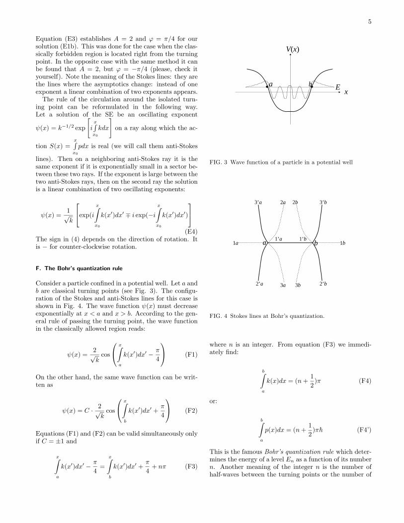
Consider a particle con�ned in a potential well. Let a andb are classical turning points (see Fig. 3). The con�gu-ration of the Stokes and anti-Stokes lines for this case isshown in Fig. 4. The wave function (x) must decreaseexponentially at x < a and x > b. According to the gen-eral rule of passing the turning point, the wave functionin the classically allowed region reads:

(x) =2pkcos

0@ xZa

k(x0)dx0 � �

4

1A (F1)

On the other hand, the same wave function can be writ-ten as

(x) = C � 2pkcos

0@ xZb

k(x0)dx0 +�

4

1A (F2)

Equations (F1) and (F2) can be valid simultaneously onlyif C = �1 and

xZa

k(x0)dx0 � �

4=

xZb

k(x0)dx0 +�

4+ n� (F3)

x

V(x)

a b E

FIG. 3 Wave function of a particle in a potential well

a b 1b

2b

3b 2’b

3’b

1’b1’a1a

2a

3a

3’a

2’a

FIG. 4 Stokes lines at Bohr�s quantization.

where n is an integer. From equation (F3) we immedi-ately �nd:

bZa

k(x)dx = (n+1

2)� (F4)

or:

bZa

p(x)dx = (n+1

2)�~ (F4�)

This is the famous Bohr�s quantization rule which deter-mines the energy of a level En as a function of its numbern. Another meaning of the integer n is the number ofhalf-waves between the turning points or the number of

6

zeros of the wave-function in the classically allowed re-gion a < x < b. The semiclassical approximation is validif n >> 1. But for practical purposes and for not toosophisticated potential the quantization rule (F40) givesrather good approximation even for the ground-state en-ergy (n = 0).The doubled value of integral (F40) is the action taken

along the closed classical trajectory S(E):

S(E) =

Ip(x)dx

Bohr conjectured in 1913 that the action S(E) is quan-tized in units of the Planck constant h = 2�~. He appliedhis conjecture to the spectrum of the Hydrogen atom andwas able to reproduce the empirical Rydberg formula forfrequencies:

!n;n0 =me4

2~3

�1

n2� 1

n02

�(n < n0)

He quantized only circular orbits, but his answer for theHydrogen spectrum was exact. It was discovered by A.Sommerfeld, who quantized elliptic orbits. The Bohrspectrum was derived rigorously by Schrödinger 13 yearslater, when he solved his equation for the Coulomb at-tractive potential.

G. An excursion to classical mechanics

The reciprocal to S(E) function E(S) can be consid-ered as the Hamiltonian in terms of the variable action.It is straightforward to prove that

@H(S)

@S=@E(S)

@S=

!

2�= � (G1)

where ! is the cyclic frequency of the orbital motion and� is the ordinary frequency. Indeed, calculation of theinverse value gives:

@S

@E=

I@p

@Edx =

Imdx

p=

Idx

v(x)= T (G2)

Here we used p =p2m(E � V (x)) and p=m =v, where

v(x) is the local velocity and T is the period of motion.Equation (G1) follows from (G2) and a trivial relation-ship T = 1=� = 2�=!. A very transparent form of equa-tion (G1) is:

@En@n

= ~! (G3)

which simply means that the classical frequency of theperiodic motion determines the energy di¤erence betweennearest levels.

What is a variable � canonically conjugated to S ? Inthe Hamiltonian formulation of classical mechanics � andS must satisfy canonical equations:

�� = @H

@S�S = �@H

@�

(G4)

Thus, for the Hamiltonian of a periodic 1-dimensionalmotion, the action S is the integral of motion and � isthe phase of motion which changes by 1 for a period.The variable ' = 2�� is the cyclic phase. The pair ofvariables � and S is similar to the pair of variables x andp. Therefore, their quantum commutator is the same:

[S; �] = ~=i (G5)

Keeping in mind that S t 2�~n and � = '=2�, we �ndthe commutator for n and ':

[n; '] = 1=i (G6)

It is identical with the commutator of the number of�phonons� n and the phase ' for the quantum oscilla-tor problem. Thus, the energy and the phase can not bemeasured simultaneously.In classical mechanics the action is an adiabatic in-

variant. It means that it is approximately invariant ifparameters of the Hamiltonian, such as the mass m orthe potential V (x), vary slowly in time. We call a valueA(t) slowly varying if its variation for the period T is

small in comparison to A, i.e.,

���� �A=A���� << �. When the

Hamiltonian depends on time, it can not be function of Sonly since the energy is not more conserved. Therefore Hdepends on � as well and the second equation of motionnow reads:

�S = �@H

@�(G7)

However, H is necessarily a periodic function of � withthe period 1. It can be represented as a Fourier-seriesconstructed by sin(2�n�) and cos(2�n�) with coe¢ cientsslowly varying in time. Averaging equation (G7) over

one period of rotation, we �nd h�Si = 0 since average of

derivative of a periodic function is zero. Note that thephase � is not an adiabatic invariant since the derivativeof the Hamiltonian by S generally has zero harmonic,i.e. a term independent on �. Its main part is given byR!(t)dt, but in the case of slowly varying parameters

there exists an additional part in zero harmonic propor-tional to the derivative @2H

@S@R (see section IV.C).

7

a b tr

FIG. 5 Quantum tunneling under a barrier.

H. The under-barrier tunneling

A classical particle with the energy E, lower than themaximum of potential energy, would be fully re�ectedfrom the classical turning point a. Due to the under-barrier penetration the quantum particle can reach thesecond turning point b and then propagate to the right(Fig. 5).Our purpose is to �nd the tunneling amplitude t. In thesemiclassical approximation the wave function must be

(x) ' tppexp

0@ i

~

xZb

pdx

1A (H1)

at x > b since right to the turning point b there is no wavepropagating to the left. This wave function grows expo-nentially under the barrier, left to the turning point b;and it is expressed by the same equation (H1) under thebarrier at a < x < b. But the same wave-function expo-nentially decreases under the barrier right to the turningpoint a. According to the general rule of passing theturning point (equation E4), the wave-function in theclassically allowed region x < a reads:

(x) ' tpp

0@e xi~Ra

pdx

� iex

� i~R

a

pdx

1A � e� i~

bRa

pdx(H2)

The statement of the problem about tunneling requiresthat the amplitude of the incident wave to be equal to 1.It means that

t = exp

0@ i

~

bZa

pdx

1A = exp

0@�1~

bZa

j p(x) j dx

1A

V(x)

xa b c

FIG. 6 Decay of a metastable state.

The probability of tunneling is:

P =j t j2= exp

0@�2~

bZa

j p(x) j dx

1A (H3)

I. Decay of a metastable state

Let us consider a potential schematically depicted inFig. 6:A classical particle with the energy E between Vmin andVmaxis con�ned on a trajectory limited by turning pointsa and b. Quantum mechanics allows the particle to tunneland escape when it reaches point b. The probability ofthis process is:

P = exp

0@�2~

cZb

j p(x) j dx

1A (I1)

as it was established in previous subsection. Let particlewas placed between a and b at an initial moment of timet = 0. The probability to �nd it in the potential wellafter time t much longer than the period of oscillationsT is:

w(t) = (1� P )t=T (I2)

At small enough P the probability (I2) can be rewrittenas:

w(t) = e�tP=T = e�2t=� (I3)

where we have introduced the life-time � of the particleon the level E:

8

� = 2T (E)=P = 2T exp

0@2~

cZb

j p(x) j dx

1A (I4)

Note, that the state of a particle in such a potentialwell is not stationary, it decays with time, but it canbe considered as being quasistationary one. It meansthat the particle makes a large number �=T oscillationsbefore it leaves. The modulus of the wave-function is de-creasing exponentially as e�t=� . The wave-function hasalso the standard phase factor exp (�iEt=~). In total

the wave-function changes in time as exp�� i(En�i )t

~

�,

where = ~=� . Thus, the metastable state can be al-ternatively described as a state with a complex energyE = En � i . The wave-function of the metastable statecan be expanded into Fourier-integral:

(t) =

Z s (E)e�iEt=~dE (I5)

The square of modulus js (E) j2can be interpreted as the

probability density to �nd our system with the energy E.A simple calculation shows that

js (E) j= const

(E � En)2 + 2(I6)

This is the so-called Lorenz distribution or the Lorenzian.It has a shape of a peak of the width centered at E =En. Thus, the metastable state has uncertainty of energy�E or the width of the level equal to . On the otherhand, its life-time � can be considered as the uncertaintyof time�t. From the relation = ~=� we �nd the energy-time uncertainty relation:

�E ��t � ~ (I7)

G. Gamov (1928) was the �rst to treat the �-decay ofradioactive nuclei as the quantum tunnelling.

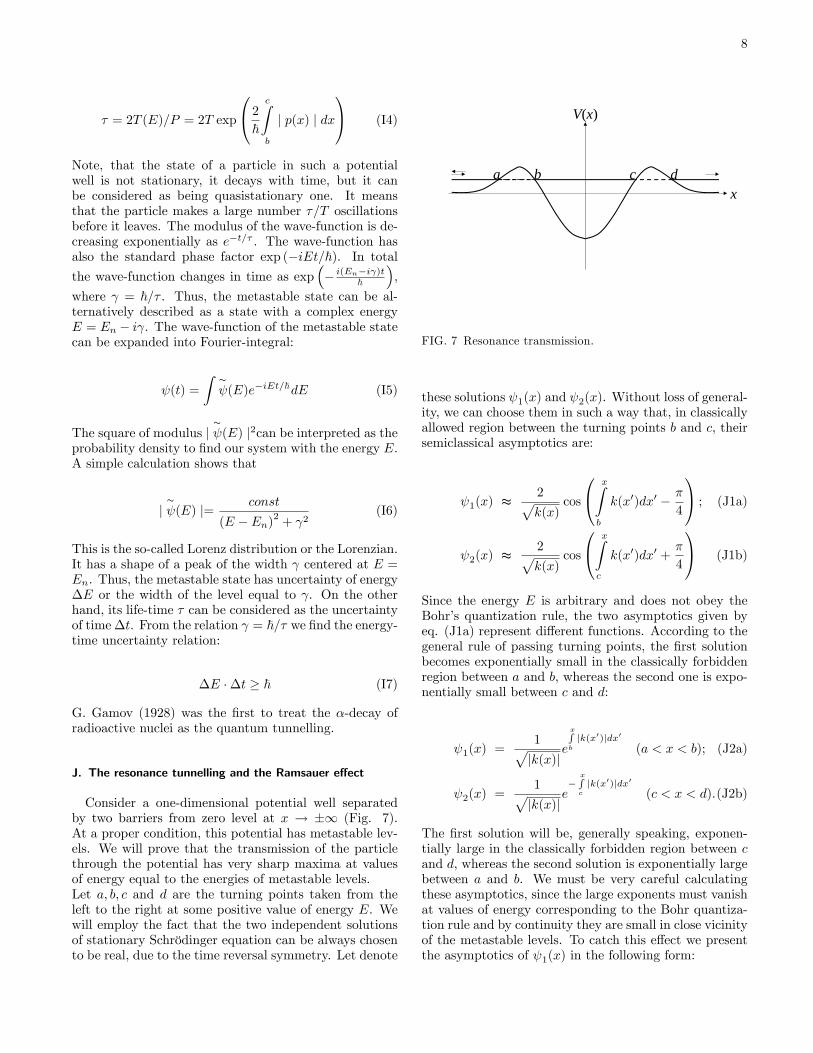
J. The resonance tunnelling and the Ramsauer e¤ect

Consider a one-dimensional potential well separatedby two barriers from zero level at x ! �1 (Fig. 7).At a proper condition, this potential has metastable lev-els. We will prove that the transmission of the particlethrough the potential has very sharp maxima at valuesof energy equal to the energies of metastable levels.Let a; b; c and d are the turning points taken from theleft to the right at some positive value of energy E. Wewill employ the fact that the two independent solutionsof stationary Schrödinger equation can be always chosento be real, due to the time reversal symmetry. Let denote

a b c d

V(x)

x

FIG. 7 Resonance transmission.

these solutions 1(x) and 2(x). Without loss of general-ity, we can choose them in such a way that, in classicallyallowed region between the turning points b and c; theirsemiclassical asymptotics are:

1(x) t2pk(x)

cos

0@ xZb

k(x0)dx0 � �

4

1A ; (J1a)

2(x) t2pk(x)

cos

0@ xZc

k(x0)dx0 +�

4

1A (J1b)

Since the energy E is arbitrary and does not obey theBohr�s quantization rule, the two asymptotics given byeq. (J1a) represent di¤erent functions. According to thegeneral rule of passing turning points, the �rst solutionbecomes exponentially small in the classically forbiddenregion between a and b, whereas the second one is expo-nentially small between c and d:

1(x) =1pjk(x)j

e

xRb

jk(x0)jdx0(a < x < b); (J2a)

2(x) =1pjk(x)j

e�

xRc

jk(x0)jdx0(c < x < d):(J2b)

The �rst solution will be, generally speaking, exponen-tially large in the classically forbidden region between cand d, whereas the second solution is exponentially largebetween a and b. We must be very careful calculatingthese asymptotics, since the large exponents must vanishat values of energy corresponding to the Bohr quantiza-tion rule and by continuity they are small in close vicinityof the metastable levels. To catch this e¤ect we presentthe asymptotics of 1(x) in the following form:

9

1(x) =2pk(x)

sin

0@ xZc

k(x0)dx0 � �

4+ �

1A ; (J3)

where � =cRb

k(x)dx. It must be a linear combination

of two solutions formally represented by sine and cosine

of the argumentxRc

k(x0)dx0 + �=4. The �rst of them de-

creases in the classically forbidden region c < x < d,whereas the second one increases. Thus, the solution 1in the forbidden region c < x < d reads:

1(x) =1pjk(x)j

"sin� e

�xRc

jk(x0)dx0+ cos� e

xRc

jk(x0)dx0#

(J4)Continuing the same solution into the right classicallyallowed region x > d, we �nd:

1(x) =2pjk(x)j

24sin� ��1R sin

0@ xZd

k(x0)dx0 � �

4

1A+cos� �R cos

0@ xZd

k(x0)dx0 � �

4

1A (J5)

where �R = exp

dRc

jk(x)dx!. The same continuation

for the solution 2 is simpler, since in the interval c < x <d it contains only one, decreasing exponent. Therefore,in the interval x > d the asymptotic of 2 is:

2(x) =2pjk(x)j

��1R sin

0@ xZd

k(x0)dx0 � �

4

1A (J6)

A linear combination of the solutions 1 and 2 whichrepresents a wave propagating to the right at x > d is:

(x) =tei�=4

2�R cos�(� 1 +

�i�2R cos�� sin�

� 2�

s teixRd

kdx0

(J7)

Here we introduced an arbitrary coe¢ cient t which occursfurther to be the transmission amplitude. Continuing oursolutions in an analogues way to the left allowed regionx < a, we �nd:

1(x) =2pjk(x)j

��1L sin

�xRa

k(y)dy + �4

� 2(x) =

2pjk(x)j

�sin� ��1L sin

�xRa

k(y)dy + �4

�� cos� �L cos

�xRa

k(y)dy + �4

�� (J8)

where �L = exp

bRa

jkjdx!. Now we are in position to

construct the asymptotic of the wave function (x) (1) atx < a. Requiring the coe¢ cient at the wave propagatingto the right to be 1, we �nd the transmission amplitude:

t =2i�L�R

(�L�R)2 cos�+ i(�2L + �2R) sin�

(J9)

Its square of modulus (the transmission coe¢ cient) is:

jtj2 = 4(�L�R)2

(�L�R)4 cos2 �+ (�2L + �2R)2 sin2 �

(J10)

Since �L;R are exponentially large values, the transmis-sion coe¢ cient (J10) reaches its maximum at cos� = 0,i.e. at energy satisfying the Bohr�s condition � = (n +1=2)�. The maximum is equal to

jtj2max =4(�L�R)

2

(�2L + �2R)2� 1

The value 1 is reached at �L = �R. The peak is verysharp. The value jtj2 decreases twice at j�2 � �j t���2L + ��2R

�. Thus, we demonstrated that the barrier

is selectively transparent for particles with energy closeto the metastable levels.The phenomenon of selective transparency was found

experimenatally in optics and electron beams propaga-tion. It is known as the Ramsauer e¤ect. It also knownas the resonant tunneling. It plays an important rolein semiconductor physics, especially in the devices calledsingle-electron transistors.

K. The overbarrier re�ection.

To �nd a small re�ection coe¢ cient for a particle withenergy higher than the maximum potential energy, onecan apply similar ideas passing the turning points x0 inthe complex plane of the coordinate x. There is no turn-ing point on the real axis, but a general theorem of com-plex variables theory guarantees that an analytical func-tion accepts any value in the complex plane. In partic-ular, V (x) = E at some point x0 of the complex plane.We consider a simple situation when there is only onesuch a point. The asymptotics of a proper wave functionare:

(x) =

�eik�x + re�ik�x x! �1teik+x x! +1 (K1)

where k� are limiting values of k(x) =p2m(E � V (x) at

x! �1, r is the re�ection amplitude, t is the transmis-sion amplitude. Starting from the real axis x at x! +1it is possible to continue the solution into the complex

10

x0

(x0)*

Re x

II

Im x

FIG. 8 Stokes lines at over-barrier re�ection.

plane of x and arrive at the line 1 ImxRx0

k(x0)dx0 = 0

which is parallel to the real axis at Rex!1 (Fig. 8).

This is possible since the potential is constant with anydesirable precision at Rex ! 1 . The asymptotic solu-tion (1) on the line 1 can be written as follows:

(x) = teik+x ttk+pk(x)

exp

0@i xZx0

k(x0)dx0

1A � (K2)� exp

0@ik+x0 � i 1Zx0

(k(x0)� k+)dx01A

The solution in this form can be continued along the line1 till the vicinity of the turning point. According to thegeneral rule (E4), the asymptotic of the same solution online 2 is

(x) =tk+pk(x)

exp

0@ik+x0 � i 1Zx0

(k(x0)� k+)dx01A �(K3)

�

24exp0@i xZ

x0

k(x0)dx0

1A� i exp0@�i xZ

x0

k(x0)dx0

1A35Passing along the line 2, we arrive at Rex ! �1 andthen descend to the real axis employing the fact that thepotential is constant with any desirable precision. Atx! �1 the argument of exponents can be evaluated asfollows:

xZx0

k(x0)dx = k�(x� x0) +xZx0

(k(x0)� k�) dx0 (K4)

� k�x�x0Z�1

(k(x0)� k�) dx0 � k�x0

Plugging (K4) into (K3) and comparing this result to thesecond line in (K1), we �nd:

tk+k�

ei

"(k+�k�)x0�

x0R�1(k(x0)�k�)dx0�

1Rx0

(k(x0)�k+)dx0#= 1

(K5)

�itk+k�

ei

"(k++k�)x0+

x0R�1(k(x0)�k�)dx0�

1Rx0

(k(x0)�k+)dx0#= r

(K6)Eliminating t from (K5) and (K6), we �nd:

r = i exp

242ik�x0 + 2i x0Z�1

(k(x)� k�) dx

35 (K7)

The integration in the argument of the exponent in (K7)can be performed along real axis x from �1 till Rex0and parallel to the imaginary axis from this point till x0.The part of argument

2ik�Rex0 + 2i

Re x0Z�1

(k(x)� k�) dx

is purely imaginary. It contributes to the phase factor.The remaining contribution is:

�2k� Imx0 � 2Im x0Z0

(k(Rex0 + iy)� k�) dy

= �2Im x0Z0

k(Rex0 + iy)dy

It has real and imaginary parts. Its imaginary part againcontributes to the phase factor only. Its real part deter-mines the modulus of r:

j r j= exp

0@�2Im x0Z0

Re k(Rex0 + iy)dy

1A (K8)

11

x

V(x)

a b­a­b

s

a

sa

Vmax

Vmin

E

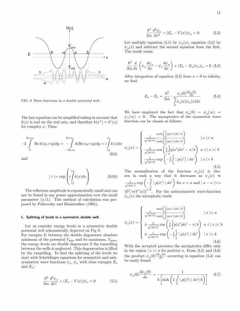
FIG. 9 Wave functions in a double potential well.

The last equation can be simpli�ed taking in account thatk(x) is real on the real axis, and therefore k(x�) = k�(x)for complex x. Thus:

�2Im x0Z0

Re k(x0+iy)dy =

Im x0

�Z

� Im x0

k(Rex0+iy)dy = i

x0Zx�0

k(x)dx

(K9)and

j r j= exp

0B@ix0Zx�0

k(x)dx

1CA (K10)

The re�ection amplitude is exponentially small and cannot be found in any power approximation over the smallparameter (�=L). This method of calculation was pro-posed by Pokrovsky and Khalatnikov (1961).

L. Splitting of levels in a symmetric double well.

Let us consider energy levels in a symmetric doublepotential well schematically depicted on Fig 9.For energies E between the double degenerate absoluteminimum of the potential Vmin and its maximum, Vmax,the energy levels are double degenerate if the tunnellingbetween the wells is neglected. This degeneration is liftedby the tunnelling. To �nd the splitting of the levels westart with Schrödinger equations for symmetric and anti-symmetric wave functions s, a with close energies Esand Ea:

~2

2m

d2 sdx2

+ (Es � V (x)) s = 0 (L1)

~2

2m

d2 adx2

+ (Ea � V (x)) a = 0 (L2)

Let multiply equation (L1) by a(x), equation (L2) by s(x) and subtract the second equation from the �rst.The result reads:

~2

2m

d

dx

� ad sdx

� sd adx

�+ (Es � Ea) s a = 0 (L3)

After integration of equation (L3) from x = 0 to in�nity,we �nd:

Ea � Es =~2

2m�

s(0)d a(0)dx

1R0

s(x) a(x)dx

(L4)

We have employed the fact that a(0) = a(1) = s(1) = 0. The asymptotics of the symmetric wavefunction can be chosen as follows:

s(x) =

8>>>>>>>><>>>>>>>>:

1pjp(x)j

cosh

�xR0

jp(x0)jdx0=~�

cosh

�aR0

jp(x0)jdx0=~� j x j< a

2pjp(x)j

cos

�1~

xRa

p(x0)dx0 � �=4�

a <j x j< b

1pjp(x)j

exp

�� 1~

xRb

j p(x0) j dx0�

j x j> b

(L5)The normalization of the function s(x) is cho-sen in such a way that it decreases as s(x) t

1pjp(x)j

exp

��aRx

j p(x0) j dx0�for x < a and j a� x j>>�

~2=mV 0(a)�1=3

. For the antisymmetric wave-function a(x) the asymptotic reads:

a(x) =

8>>>>>>>><>>>>>>>>:

1pjp(x)j

sinh

�xR0

jp(x0)jdx0=~�

sinh

�aR0

jp(x0)jdx0=~� j x j< a

� 2pjp(x)j

cos

�1~

xRa

p(x0)dx0 � �=4�

a <j x j< b

� 1pjp(x)j

exp

�� 1~

xRb

j p(x0) j dx0�

j x j> b

(L6)With the accepted precision the asymptotics di¤er onlyin the region j x j< a for positive x. From (L5) and (L6)the product s(0)

d a(0)dx occurring in equation (L4) can

be easily found:

s(0)d a(0)

dx=

1

~�sinh

�2

aR0

j p(x0) j dx0=~�� (L7)

12

Let calculate the integral:

1Z0

s(x) a(x)dx tbZa

s(x) a(x)dx t

t 4

bZa

cos2

24 xZ0

p(x0)dx0=~� �=4

35 dx

p(x)

Substituting quickly oscillating cos2 by its average value1/2, we arrive at a following result:

1Z0

s(x) a(x)dx tb

2

Za

dx

p(x)=1

mT (E) (L8)

where T (E) is the period of motion along the classicaltrajectory. Plugging (L7) and (L8) into equation (L4),we obtain:

Ea � Es =~

T (E)

�sinh

�2

aR0

j p(x0) j dx0=~�� t(L9)

t~!�exp

0@� aZ�a

j p(x0) j dx0=~

1Awhere ! is the classical frequency of motion ( ~! is thedistance between levels in each well). Again we obtainexponentially small value, speci�c for a classically forbid-den e¤ect. Note that the antisymmetric state has alwayshigher energy than the symmetric one.

M. Semiclassical approximation for the radial waveequation

The radial SE for spherically symmetric potentialreads:

1

r2d

dr

�r2d

dr

�+

�k2 � v(r)� l(l + 1)

r2

� = 0 (M1)

where as usual k2 = 2mE=}2 and v(r) = 2mV (r)=}2.The last term is proportional to centrifugal potential;the integer l is the dimensionless total orbital momen-tum. We assume l� 1. To trasform this equation to thestandard one-dimensional form we introduce a new func-tion �(r) = r (r). The wave equation for the function �reads:

d2�

dr2+

�k2 � v(r)� l(l + 1)

r2

�� = 0 (M2)

General condition of semiclassical approximation also re-quires that

dk(r)

dr� k2(r); k(r) =

rk2 � v(r)� (l + 1=2)

2

r2(M3)

Note that the centrifugal term in expression (M3) for k(r)di¤ers from that in equation (M2) by a comparativelysmall term 1=4r2. We will show later that this choice al-lows to obtain an interpolation formula which works wellat large and small values of r. Indeed, if the potentialvaries slowly enough and r � k=l, the requirement (M3)is satis�ed. At r � k=l the centrifugal term dominates.Then k(r) becomes purely imaginary k(r) t �i(l+1=)=r.The wave function � decreasing in the classically forbid-den area r < r0 reads:

�(r) =ei�=4pk(r)

exp

0@i rZr0

k(r0)dr0

1A (M4)

where r0 is the classical turning point. For r � l + 1=2the approximate estmate is

�(r) tr

r

l + 1=2exp

�(l + 1=2) ln

r

l + 1=2

�=

�r

l + 1=2

�l+1For the initial radial wave function in the same region we�nd an asymptotic:

(r) trl

(l + 1=2)l+1

which agrees with the general analysis. Then in classi-cally allowed region r > r0 the semiclassical approxima-tion reads:

�(r) =2pk(r)

sin

0@ rZr0

k(r0)dr0 +�

4

1A (M5)

Problems:1. Find asymptotics of spherical Bessel functions jl(x)

at large values of l.2. The same problem for standard Bessel functions.3. Find the roots xn;m of Bessel functions Jm(x) with

large m or with large n or both.

III. SEMICLASSICAL APPROXIMATION IN 3DIMENSIONS

A. Hamilton-Jacobi equation

Solving Schrödinger equation in 3 dimensions for thecase when j r� j= (� jrV j =K) << 1, we apply the same

13

FIG. 10 Family of classical trajectories.

trick representing as = eiS=~. Equation for S(r;E)reads:

1

2m(rS)2 + V (r)� i~

2m�S = E (A1)

Again we expand formally S into a power series over ~:

S = S0 + ~S1 + ~2S2 + ::: (A2)

Then in the leading approximation we �nd equation forS0:

1

2m(rS0)2 + V (r) =E (A3)

This equation is well-known in classical mechanics as thestationary Hamilton-Jacobi equation. It can be consid-ered as one of possible formulations of classical mechan-ics, equivalent to other important formulations: New-ton laws, Hamilton canonical equations and Lagrange-Hamilton variational principle. As it is seen from equa-tion (3), the value 1

2m (rS0)2 is the kinetic energy of a

particle. Therefore, the absolute value of rS0 is equalto the absolute value of momentum at the point r for aparticle with the total energy E. To understand whatis the physical meaning of the function S0(r) consider afamily of trajectories for particles with �xed energy pass-ing through a point r0 of a surface � with the directionof velocity n0= v0=jv0j normal to the surface (see Fig.10). The modulus of the velocity for each starting pointr0 is uniquely de�ned as p(r0)=m.

One can imagine the surface � as a set of points r0 passedby a beam of particles at some initial moment of time t0.These conditions determine a family of trajectories r(t) =

r(t; r0; E) unambiguously. The classical action along thistrajectories is:

S(r;E) =

rZr0

p(r0)dr0 (A4)

At a �xed surface � the point r0 is determined by thepoint r 3 . Therefore, S(r;E) is a function of r only. Itsgradient is equal to the momentum of a particle on atrajectory starting on � in the point r0 with the velocityperpendicular to �. The surface S(r;E) =const is normalto the family of trajectories intersecting this surface. Inoptics the surface perpendicular to the light rays is calledthe wave front. A close analogy between the Hamilton-Jacobi formulation of classical mechanics and the di¤rac-tion theory of optical waves inspired W.R. Hamilton todevelop his particle-wave analogy which anticipated theQuantum Mechanics more than half a century prior itscreation.Equation (A4) shows how to construct a general solu-

tion of the Hamilton-Jacobi equation4 . One should �x asurface � in 3d space (or a line in 2d space) and �nd theunit vector of normal n0(r0) at each point of this sur-face, then calculate classical trajectories passing through� with the direction of velocity n0(r0), �nd a trajectorypassing through the point r and integrate momentumalong this trajectory. It is clear that the general solutionS(r;E) depends on the choice of initial surface �, whichis completely determined by an arbitrary function of 3(or 2) variables. On the other hand, any particular so-lution of Hamilton-Jacobi equation (A3) corresponds toa family of classical trajectories which can be found assolution of ordinary di¤erential equation:

�r(t) =

1

mrS(r) (A5)

As an example, consider free particles (V (r) =0). A sim-plest solution of equation (3) in this case is

rS0 = p = const; S0 = p � r (A6)

It corresponds to a family of straight-lined trajectoriesparallel to the constant vector p. The initial surface � isthe plane perpendicular to p. The wave-function corre-sponding to this solution is the plane-wave (r) =eip�r=~.This result seems quite natural. A spherically symmetric

3 Actually, it can happen that several trajectories starting at di¤er-ent r0 pass through the same point r. We consider this situationlater.

4 The method described here is well known in theory of di¤erentialequations with partial derivatives as �Method of characteristics�.

14

solution of Hamiltonian-Jacobi equation for a free parti-cle is:

S = p � r (A7)

where p is a constant and r is the spherical radius. Its

gradient rS = p^r is directed along the radius and its

modulus is constant. The initial surface � is a sphere. Inclassical mechanics this solution corresponds to a beamof particles moving from the origin with a permanentvelocity. In quantum mechanics it is an outgoing spher-

ical wave (r) =exp( ipr~ )

r . The origin of the factor r indenominator is explained in the next subsection. Thereader can construct cylindrical wave in a similar way.Note that trajectories in both cases have no intersections.

B. The caustics and tubes of trajectories

A less trivial situation arises when trajectories inter-sect. As an example consider trajectories of free particlesin 2 dimensions starting from a parabola y = kx2 in thedirection normal to the parabola in the starting point(Fig. ??) .If the coordinates of starting point are y0 = kx20 and x0, equation of the trajectory is:

y � kx20 = �1

2kx0(x� x0) (B1)

Equation (B1) can be considered as equation for x0 at�xed x and y. It has only one root for any point betweenthe initial parabola y = kx2 and a curve

x = �2(2ky � 1)3=2

3p6k

(B2)

For any point (x; y) inside the latter curve (�semicubicparabola�) there exist three trajectories passing throughit (try to prove this statement). The curve (B2) is theenvelope of classical trajectories, the so-called caustic.Even visually it is seen as a line where classic trajecto-ries become dense. Therefore, one can expect that thestationary density increases near caustics. This anticipa-tion will be supported by the direct calculation later.As a second example let us consider particles in 2 di-

mensions subjected to an external potential V (x) de-pending on coordinate x only. The family of trajectoriesis characterized by the total energy and the angle � whichthey form with the x-axis at x! �1 where V (x) can beneglected. The components of momentum in this asymp-totic region are px =

p2mE cos � and py =

p2mE sin �.

The value py is conserved. Therefore

p2x = 2mE � p2y � 2mV (x) = 2m(E cos2 �� V (x)) (B3)

FIG. 11 Trajectories of particles and caustics in a parabolicbilliard.

V(x)=Ecos2θ

x

FIG. 12 Caustics for a 2d particles in 1d potential.

It becomes zero at V (x) = E cos2 � < E . This is againthe envelope of classical trajectories for this case, i.e. thecaustic (Fig. 12).Note,that the energy remains larger than the potentialenergy, but the region behind the caustic V (x) > E cos2 �is classically forbidden. Thus, the caustics can be alsoconsidered as boundaries of classically allowed regions.The classically forbidden region behind a caustic is theshadow region in optics and common life.Now we proceed to construction of the next after the

leading semiclassical approximation. Returning to equa-tion (A1), we retain in it terms proportional to ~. Theresult reads:

2rS0rS1 = i�S0 (B4)

15

A1

A2

FIG. 13 Tube of trajectories.

Remembering that rS0 = p, equation (B4) can berewritten as follows:

(pr)S1 =i

2r � p (B5)

Let us introduce a coordinate along a classical trajectory.As the most natural choice for the coordinate along thetrajectory we accept its length l from some initial point tothe current point. Then equation (B5) can be rewrittenin an equivalent form:

dS1dl

=i

2pr � p (B6)

To solve it explicitly, we need to elucidate the geomet-rical meaning ofr�p. Consider a tube limited by a familyof trajectories and cut it by two close cross-sections 1 and2, normal to trajectories (Fig. 13).The �ux of the vector p through a surface composed bythese cross-sections and the tube of trajectories connect-ing them is equal to p1A1 � p2A2 where p1;2 are valuesof the momentum at the cross-sections 1 and 2 and A1;2are the cross-section areas. Since p is directed along tra-jectories, there is no �ux through the side part of thesurface. The volume limited by our surface is approxi-mately equal to A ��l where �l is the distance along thetrajectories between the cross-sections. Therefore:

r � p = lim�l!0

p1A1 � p2A2A�l

=1

A

d(pA)

dl(B7)

Substituting (B7) into (B6) and integrating both partsby l, we �nd:

S1 =i

2(ln pA� lnC) (B8)

where C is a constant. To make S1 �nite, this constantmust be proportional to a cross-section area A0 at somepoint. Then equation (B8) acquires a �nite limit whenthe tube of trajectories becomes in�nitely thin: the ratioof cross-sections at di¤erent points of trajectory is �nite.Plugging S0and S1 into the wave function = eiS=~, we�nd:

(x) =CppA

exp

0@ i

~

xZx0

pdx

1A (B9)

where the integration proceeds along a classical trajec-tory. The pre-exponential factor ensures that the �uxof particles through the cross-section of a narrow tube oftrajectories does not change from one cross-section to an-other, i.e. that the number of particles or their probabil-ity is conserved. In particular, for spherical way A � r2

leading to the factor r in denominator.Since a narrow tube of trajectories merges into a point

on a caustic, equation of the caustic can be formulated asA = 0. Equation (B9) shows that the semiclassical wave-function has a singularity near caustics and the densitygrows as 1=A. Actually, equation (B9) is invalid in asmall vicinity of the caustic. In terms of a coordinate� perpendicular to the caustic and equal to zero exactlyon it, the validity of semiclassical approximation (B9) re-quires that j�j >> ~2=3=(m j rV j)1=3, similar to whatwas found in 1d case. Close inspection reveals the ruleof passing through the caustic also similar to that wefound for passing the turning point in 1d . In particular,the wave-function decreases exponentially in classicallyforbidden region (shadow region). If several classical tra-jectories pass through the point x, as it has happened inabove considered examples, equation (B9) must be gen-eralized:

(x) =Xj

CjppjAj

exp

�i

~Sj(x)

�(B10)

where j enumerates the trajectories.

C. Bohr�s quantization in 3 dimensions. Deterministicchaos in classical and quantum mechanics

Generalization of the Bohr�s quantization rule (1.F4�)is obvious:

S(E) =

Ipdx = (n+ )~ (C1)

where integral is taken along a closed trajectory and is aconstant of the order of one. The necessary conditions forsuch a quantization is the existence of classical periodictrajectory.

16

How restrictive is this limitation? This problem is veryimportant for classical mechanics. There exist few excep-tional systems which allow the exact solution of the New-ton or Hamilton equations due to their high symmetry.One of the most important is the Kepler (or Coulomb)problem. In this case the periodic solutions are found ex-plicitly. But how do they relate to reality? Real systemsalways are subject to perturbations which destroy thesymmetry. For example, the Earth rotates in the grav-itational �eld of the Sun, just the Kepler problem. Butit is also e¤ected by the moon and other planets. Canit happen that in the course of time these perturbationsare accumulated and destroy the Keplerian periodicity?The answer to this question was given by French

matematician A. Poincare and later by A. Kolmogorov,V. Arnold and A. Mozer. They have found that a weakperiodic perturbation does not destroy periodic trajec-tory if the ratio of the perturbation frequency to the fre-quency of motion on the trajectory is not close to a ratio-nal number with su¢ ciently small nominator and denom-inator, i.e. they are not in resonance. If, on contrary, theperturbation frequency is close to a low-order resonanceor its amplitude is large, the initial classical trajectorycan be destroyed. It becomes aperiodic, though it can belimited in space. In this situation two trajectories withvery close initial conditions diverge very far in the courseof time. It means, that the coordinates and momentabecome unpredictable. The motion becomes chaotic, de-spite of the fact that equations of motion are completelydeterministic. This is the so-called deterministic chaos,the main problem of the modern non-linear mechanics.How the deterministic chaos displays itself in the quan-

tum mechanics? One can conjecture that the random-ness of trajectories lead to the randomness of phase fac-tors for wave-functions and transition amplitudes. Notonly phase factors, but the moduli of transition ampli-tudes become random since the caustics also are chaotic.Thus, in quantum mechanics the matrix of transitionamplitudes is random. The transition amplitudes arematrix elements of the evolution operator U(t). SinceU(t) = exp (iHt=~), it also means that the HamiltonianH can be considered as a random matrix. Theory of ran-dom matrices was created by E. Wigner and F. Dyson. Itshows that the distance � between nearest energy levels

is a random value. Its average�� is equal to inverse den-

sity of levels (@n=@E)�1, but its �uctuations are of thesame order of magnitude. The probability density to �ndthe inter-level distance � occurs an universal function of

the ratio �=��. This function is now reliably established.

It plays the central role in so remote areas as spectra ofatomic nuclei, spectroscopy of highly excited (Rydberg)atoms in external magnetic �eld and properties of disor-dered conductors of small size (the so-called mesoscopic).Among numerous books and reviews on classical and

quantum deterministic chaos I can recommend the bookby M. Gutzwiller (5).

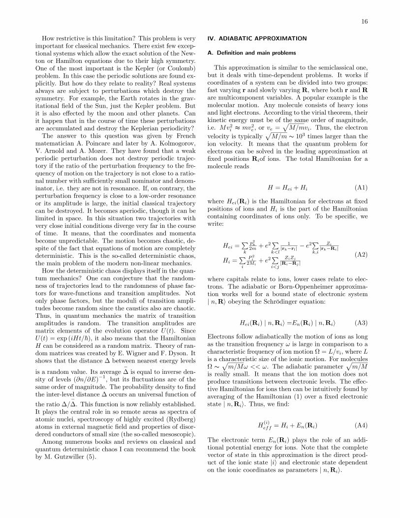
IV. ADIABATIC APPROXIMATION

A. De�nition and main problems

This approximation is similar to the semiclassical one,but it deals with time-dependent problems. It works ifcoordinates of a system can be divided into two groups:fast varying r and slowly varying R, where both r and Rare multicomponent variables. A popular example is themolecular motion. Any molecule consists of heavy ionsand light electrons. According to the virial theorem, theirkinetic energy must be of the same order of magnitude,i.e. Mv2i t mv2e , or ve =

pM=mvi. Thus, the electron

velocity is typicallypM=m s 103 times larger than the

ion velocity. It means that the quantum problem forelectrons can be solved in the leading approximation at�xed positions Riof ions. The total Hamiltonian for amolecule reads

H = Hei +Hi (A1)

where Hei(Ri) is the Hamiltonian for electrons at �xedpositions of ions and Hi is the part of the Hamiltoniancontaining coordinates of ions only. To be speci�c, wewrite:

Hei =Pk

p2k2m + e

2Pk<l

1jrk�rlj � e

2Pk;i

Zijrk�Rij

Hi =Pi

P 2i

2Mi+ e2

Pi<j

ZiZjjRi�Rj j

(A2)

where capitals relate to ions, lower cases relate to elec-trons. The adiabatic or Born-Oppenheimer approxima-tion works well for a bound state of electronic systemj n;Ri obeying the Schrödinger equation:

Hei(Ri) j n;Rii =En(Ri) j n;Rii (A3)

Electrons follow adiabatically the motion of ions as longas the transition frequency ! is large in comparison to acharacteristic frequency of ion motion = L=vi, where Lis a characteristic size of the ionic motion. For molecules s

pm=M! << !. The adiabatic parameter

pm=M

is really small. It means that the ion motion does notproduce transitions between electronic levels. The e¤ec-tive Hamiltonian for ions then can be intuitively found byaveraging of the Hamiltonian (1) over a �xed electronicstate j n;Rii. Thus, we �nd:

H(i)eff = Hi + En(Ri) (A4)

The electronic term En(Ri) plays the role of an addi-tional potential energy for ions. Note that the completevector of state in this approximation is the direct prod-uct of the ionic state jii and electronic state dependenton the ionic coordinates as parameters j n;Rii.

17

Another example is delivered by a particle with spin1/2 moving slowly in varying in space magnetic �eld B.Then the transition frequency is ! = g�BB=~ where�B =

e~2mc is the Bohr magneton, g is the gyromagnetic

ratio (2 for a free electron). The adiabaticity conditionreads:

v=L << ! (A5)

where v is the particle velocity. In this case the direc-tion of spin follows adiabatically the local direction ofmagnetic �eld being either parallel or antiparallel to it.One more example is delivered by a quantum rotator

, i.e. a particle with large spin or total angular momentJ; placed into external electric or magnetic �elds. Thecentre of the particle must be �xed. Classical rotator ischaracterized by its two spherical coordinates � and '.They play role of slow coordinates. The fast coordinatesdetermine quantum �uctuations of the rotator near theclassical position. We will return to this example in somedetails later.General formulation of the adiabatic approximation is

as follows. Let the Hamiltonian of a systemH(R) dependon a set of parameters R which vary in time. Let j n;Riis a stationary state of this Hamiltonian at a �xed set R:

H(R) j n;Ri = En(R) j n;Ri (A3�)

The process is called adiabatic if

j�R jj R j <<

En+1 � En~

= ! (A4)

Since transitions are suppressed in the adiabatic process,it is obvious that the system will follow the same statej n;Ri as long as adiabaticity condition (4) is satis�ed.Two main problems must be solved to complete the pic-ture.i) The adiabatic approximation de�nitely is invalid inpoints where two or more levels cross, since transitionfrequency ! turns into zero. Then the transition be-tween levels become probable. The problem is to �ndthe transition amplitudes. This is the so-called Landau-Zener problem. Points of levels crossing in the adiabaticproblem are similar to the classical turning points in thesemiclassical approximation.ii) The electronic state j n;Ri persists if R vary veryslowly with time, but it does not exclude a time-dependent phase factor ei (t) accompanying the adiabaticchange of parameters R. This phase is called the Berry�sphase. It plays very important role in numerous inter-ference phenomena. It also changes the e¤ective Hamil-tonian for slow variables R.

1

12

2

|V|t

FIG. 14 Two levels crossing. Dashed lines show levels in theabsence of interlevel matrix element. Solid lines show levelsin adiabatic approximation.

B. Transitions at avoided two-level crossing (Landau-Zenerproblem)

Though sometimes more than two levels can cross si-multaneously, two-levels crossing is the most common sit-uation. At two-level crossing we can neglect all other lev-els and consider two-level system. We start with the con-sideration of the most general two-level system with thetime-independent Hamiltonian. Stationary Schrödingerequations for such a system are:

�E1a1 + V a2 = Ea1V �a2 + E2a2 = Ea2

(B1)

where a1;2 are the amplitudes of the states, E1;2 are theirenergies and V is the transition matrix element. Solutionof secular equation for the system (1) reads:

E� =E1 + E2

2�r(E1 � E2)2

4+ j V j2 (B2)

If j E1 � E2 j>> V , the two solutions (2) are approxi-

mately E+ = E1 +jV j2

E1�E2 , E� = E2 � jV j2E1�E2 , very close

to initial levels E1, E2. In the opposite limiting casej E1 � E2 j<< V , we �nd E� t E1+E2

2 � j V j. It meansthat energy levels do not cross, they repulse each otherand the minimal distance between them is 2 j V j. Thisphenomenon is called the Wigner-Teller level repulsion.If E1 and E2 are driven by some parameter t, a schematicpicture of levels near the crossing looks like it is shownon Fig. 14.At in�nitely slow variation the system followsthe static level which it occupied initially. It means thatthe state 1 transits with the probability 1 to the state2 and vice versa. Most naturally one can choose t to

18

be real time. The time-dependent Schrödinger equationsmust be solved. They are:

(i~ �a1 = E1(t)a1 + V a2

i~ �a2 = E2(t)a2 + V

�a1(B3)

By the change of variables:

a1;2 = exp

0@� i~

tZt0

E1(t0) + E2(t

0)

2dt0

1Asa1;2 (B4)

the system (3) is reduced to a following one:

i�~a1 =

!(t)2 ~a1 + v~a2

i�~a2 = �!(t)

2 ~a2 + v�~a1

(B5)

where !(t) = (E1(t) � E2(t))=~ is the time-dependenttransition frequency and v = V=~. We are interested in avicinity of the levels crossing point only. Accepting t = 0in this point, let expand the frequency up to a linearterm: !(t) =

:!0t , where

�!0is the time derivative of the

frequency at the crossing point. The time dependence ofv can be neglected. In this approximation the system (5)can be rewritten as:

(i�a1 =

�!0t2 a1 + va2

i�a2 = v�a1 �

�!0t2 a2

(B5�)

Here and further we omit tilde over a1;2:In terms of a

dimensionless variable � =q

�!0t equation (5�) reads:

� �i dd� �

�2

�a1 = a2�

i dd� +�2

�a2 = �a1

(B6)

These equations depend on one dimensionless parameter = vp

�!0= V

~p

�!0which was �rst introduced by Landau

(without loss of generality v can be taken real, ascribingits phase factor to a2). It is possible to eliminate the am-plitude a2 from the system (6) and reduce it to a secondorder di¤erential equation for a1:

�id

d�+�

2

��id

d�� �

2

�a1 =j j2 a1 (B7)

or

d2a1d�2

+

�i

2+�2

4+ j j2

�a1 = 0 (B8)

This is the so-called equation of parabolic cylinder. Itstwo independent solutions are expressed in terms of thecon�uent hypergeometric functions, but our purpose can

be achieved without knowledge of these special functions.We look for a solution which corresponds to the �lledstate 1 and empty state 2 at t ! �1, i.e. j a1 j= 1and a2 = 0 at � ! �1. Neglecting j j2 in equation(8) at large j � j, we �nd two independent solutions ofequation (8): a(1)1 t e�i�

2=4, a(2)1 t ei�2=4

� . Only the �rstone corresponds to our initial condition at � ! �1, thesecond one leads to a �nite a2 according to (6). To �ndwhat happens with this solution at � ! +1, we applythe same trick we have used already for passing the clas-sical turning point: we pass the crossing point � = 0along a big circle in the upper half-plane of the complexplane � . To understand why the contour of circulationmust be chosen in the upper half-plane, let us considerthe asymptotic behavior of the solution a1 t e�i�

2=4.This solution decreases exponentially on the Stokes linearg � = 3�=4. Therefore, it de�nitely is represented bythe same exponent on the ray arg � = � and on a largearc in the complex plane � until it crosses the secondStokes ray arg � = �=4. After this line a second asymp-totic solution must be added with the coe¢ cient �i, butthe coe¢ cient at the �rst one does not change till thenext Stokes line arg � = ��=4 and the second solutionvanishes on the real axis at � ! +1. Due to the ad-ditional term j j2 a1 in equation (7), the modulus ofthe solution a1 is not more equal to 1 at � ! +1. In-deed, representing a1 as a1 = eiS(�) in the spirit of thesemiclassical approximation, we �nd equation for S(�):

�dS

d�

�2� id

2S

d�2=

��2

4+i

2+ j j2

�(B9)

At large � we expand dSd� in a series over

1� . In the leading

approximation we �nd:

dS0d�

= ��2; S0 = �

�2

4(B10)

Next approximation reads:

2dS0d�

dS1d�

=j j2 ; S1 = � j j2 ln � + const (B11)

If the constant in equation (11) is chosen to make S1real at arg � = +�, then ImS1 = � j j2 at arg � = 0.Therefore,

j a1 j= e��j j2

at � ! +1 (B12)

Pay attention to the fact that, if we formally perform acirculation in the lower half-plane of � , we obtain an er-roneous answer for asymptotic value a1 = e�j j

2

(j a1 jcan not be more than 1). This asymmetry stems fromthe exponential growth of the solution e�i�

2=4along theStokes line arg � = �i3�=4. It acquires another exponent

19

on the line arg � = �i�=2 which further grows exponen-tially, while the initial exponent becomes uncontrollablysmall. The result (12) was �rst obtained independentlyby Landau and Zener in 1932.Landau has added to this consideration a feature spe-

ci�c for electronic transitions at a collision of two atomsor ions. In this case the adiabatic parameter is the dis-tance R between colliding particles. Let the level cross-ing takes place at some value R = R0. Then it happenstwice during the collision process provided the minimaldistance between the particles Rmin is less than R0. Letthe crossing proceeds at moments of time t1 and t2. If

the change of phaset2Rt1

!(t)dt between the crossing is large,

the interference e¤ects are negligibly small at small aver-aging over energy or other quantum numbers. Then notthe amplitudes, but the probabilities of di¤erent versionsof electronic transitions become additive. The transitionprobability at one crossing is P = 1� j a1 j2. The transi-tion probability at the collision Pcol is the sum of prob-abilities that the transition happens at the �rst crossingand does not happen at the second one and vice versa,i.e.

Pcol = 2P (1� P ) = 2e�2�j j2�1� e�2�j j

2�

(B13)

An interesting problem of interference between two suc-cessive transitions is not yet solved.

C. Berry�s phase, Berry�s connection

1. De�nition of the geometrical phase

Let us consider again a system with adiabatically vary-ing parameters R(t) and with the Hamiltonian H(R):Let En(R) and j n;Ri are the eigenvalues and corre-sponding eigenstates of the Hamiltonian H(R). We willlook for a solution of the time-dependent Schrödingerequation:

i~@

@tj �; ti = H(R(t)) j �; ti (C1)

considering�R(t) as small values: j

�R(t)jR << !n;n�1.

Then, as it was already argued, the interlevel transi-tions are suppressed and time-dependent states presum-ably follow stationary states j n;R(t)i corresponding toinstantaneous values of the parameters. Thus, a solutionof equation (C1) generically associated with j n;R(t)ican be represented as

j n; ti = e�i'(t) j n;R(t)i (C2)

By such an ansatz we automatically provide a correctnormalization of the state j n; ti. Substituting (2) to (1),we arrive at equation:

~@'

@tj n;R(t)i+i~ @

@tj n;R(t)i =En(R(t)) j n;R(t)i

(C3)What is lost in this approach is the admixture of othereigenstates j n0;R(t)i (n0 6= n) generated by the deriva-tive

@

@Rj n;Ri =

Xhj n0;Rin0

hn0;R j @@R

j n;Ri

It determines the transition amplitudes, i.e. the Landau-Zener problem. In this section we assume that the tra-jectory R(t) passes su¢ ciently far from the level crossingpoints and neglect the transitions. Note,that even if itpasses the crossing point, the Landau-Zener parameter

2 =V 2

~2j �!j'

�R2

j hn0;R j @@R j n;Ri j2

~2 j @!=@R jj�R j

s�R

goes to zero when

���� �R���� goes to zero. Thus, the transi-tion amplitudes are zero in adiabatic limit, whereas theBerry�s phases are �nite. Let multiply equation (C3) byhn;R(t) j to �nd:

@'

@t=1

~En(R(t))� ihn;R(t) j (

@

@tj n;R(t)i) (C4)

We prove that the second term in the r.-h.s. of equation(C4) is real. Indeed, from the normalization conditionhn;R(t) j n;R(t)i = 1 it follows that

hn;R(t)( @@tj n;R(t)i) + ( @

@thn;R(t) j) j n;R(t)i = 0

On the other hand, according to general relations:

(@

@thn;R(t) j)jn;R(t)i = hn;R(t) j ( @

@tjn;R(t)i�

Thus, the matrix element hn;R(t) j ( @@t jn;R(t)i) is anumber equal to its complex conjugated taken with thesign minus and, therefore, it is purely imaginary. Return-ing to equation (C4), let integrate it:

'(t) =1

~

tZt0

En(R(t0))dt+ (t; t0) (C5)

where

(t; t0) = �t

i

Zt0

hn;R(t0) j @@t0jn;R(t0)idt0 (C6)

20

The �rst part of the phase '(t) is what we could expectfrom the naive arguments similar to those used for ex-planation of the semiclassical limit. But the second part (t; t0) is not trivial. It is called the Berry�s phase inhonor of the author, Michael Berry, who has discoveredit in 1983. This is an example of a simple phenomenonwhich was overlooked by numerous researchers during al-most 50 years after discovery of Quantum Mechanics.We will simplify equation (6). First, let us note that

hn;R(t) j @@tn;R(t)i = dR

dt� hn;R(t) j @

@Rj n;R(t0)i

Thus, equation (6) can be rewritten as follows:

(t; t0) =

tZt0

A(R(t))dR

dt� dt (C7)

where we have introduced the so-called Berry�s connec-tion:

A(R) = �ihn;R j @

@Rj n;Ri (C8)

Since dRdt � dt = dR, the integral in (C6) can be trans-

formed into a linear integral along a trajectory R(t):

(t; t0) = (R;R0) =

RZR0

A(R0(t))dR0 (C9)

The last equation demonstrates that the Berry�s phaseis a geometrical phase in the meaning that it dependson the shape of trajectory and its endpoints, but it doesnot depend on the dynamics on the trajectory. Any timedependenceR(t) at passing a �xed curve inR-space leadsto the same Berry�s phase. Therefore, the Berry�s phaseis also called the geometrical phase.An important peculiarity of the Berry�s phase C9 is

that the Planck constant is dropped out of it. It meansthat the Berry�s phase is a purely classical e¤ect. Itsphysical meaning can be easily explained for a simpleexample of the Foucault pendulum. It is well knownthat its oscillation is followed by a slow rotation of theoscillation plane due to the Coriolis force induced by theEarth rotation around its axis. The Berry�s phase is thephase of this rotation for this speci�c problem.More generally, the classical adiabatic motion is a fast

oscillation with slowly varying parameters. The fre-quency of this motion is a given function of time, but itsphase and amplitude also vary slowly (see section II.G).

2. Gauge transformations

The geometrical phase (R;R0) is not de�ned uniquelyeven if the contour of integration is �xed together with

R0

R

FIG. 15 Trajectory of a system in R-space.

its ends. Multiplication of the ket j n;Ri by a phase fac-tor e�if(R) depending on R and the simultaneous gaugetransformation of the Berry�s connection:

A(R)! A(R) +rRf(R) (C10)

does not change the time dependence of the state j n; ti.The gauge transformation of the Berry�s phase reads:

(R;R)! (R;R0) + f(R)� f(R0) (C11)

The gauge transformation of the Berry�s connection (10)is similar to the gauge transformation of the vector-potential in electricity and magnetism theory. It isnot surprising since both �elds belong to the class ofthe Yang-Mills gauge �elds compensating the local U(1)transformation5 . An essential di¤erence between themis that the electromagnetic vector-potential depends onreal coordinates r, whereas the Berry�s connection de-pends on parameters R which can be identi�ed withslow variables. Thus, the Hamiltonian for slow vari-ables must include A(R) in a gauge-invariant combi-nation rR = 1

i @=@R�A which is proportional to the

quantum operator of velocity�R. Indeed, according to

the adiabatic assumption, a state of the complete systemjS; F i including fast and slow variables is a direct prod-uct of the type: jS; F i = jSi jn;Ri in which the �rstket determines the state of slow subsystem and the sec-ond ket is the state of the fast subsystem parametrically

5 In terms of topological �ber-bundles theory the gauge potentialrealises connection (parallell translation) between U(1) layers be-longing to di¤erent points of the base (the manifold of points la-beled by R). It justi�es the notation �Berry�s connection�, butmay be �Berry�vector-potential�would be not worse.

21

dependent on slow coordinates. Applying the translationgenerator �i @=@R to this state and multiplying the re-sulting state by the bra hRj hn;Rj where hRj is thevector of a state with a �xed coordinate, we arrive at thegauge invariant derivative:

1

i

@ (R)

@R�i (R)� hn;Rj @

@Rj n;Ri = (1

i

@

@R�A(R)) (R)

Here (R) = hR jSi is the Schrödinger wave-function forslow coordinates.

3. Invariant Berry�s phase

Though generally the Berry�s phase is not invariantunder the gauge transformation, it becomes invariant forany closed contour C. In this case the gauge phases f(R)and f(R0) coincide and cancel each other (see equation(C11). Thus, for a closed contour the geometrical phasedepends only on the contour: = (C). Here we �ndthis dependence in some important cases.We start with the case of a particle with spin 1/2 mov-

ing in an inhomogeneous magnetic �eld. The spin Hamil-tonian for such a system is:

HB(B) =g�Bs �B (C12)

and B is an arbitrary slow function of time t. Slow here

means that j�B j =B � g�BB=~. The vector B plays the

role of slow parameters which was denoted in previoussections R. The spin adiabatically follows the directionof magnetic �eld B: The instantaneous stationary states

are spinors j �;^

Bi obeying equations:

^

B � s j �;^

Bi = �12j �;

^

Bi (C13)

(^

B is unit vector along magnetic �eld B). Let us ex-pand them in a �xed base j �1=2; zi of states with spinprojections �1=2 onto a �xed axis z:

j �;^

Bi = ��(^

B) j+; zi+ ��(^

B) j�; zi (C14)

Substituting (3) into (2) and solving corresponding equa-tions, we �nd: �+ = cos �=2; �+ = sin �=2 e�i';�� = sin �=2 e

i'; �� = cos �=2 where � and ' are spheri-

cal angles determining the direction of^

B. It is convenientto express �� and � � directly in terms of Cartesian com-ponents of the vector B:

�+ =

rB +Bz2B

; �+ =

rB �Bz2B

Bx � iByqB2x +B

2y

(C15)

�� =

rB �Bz2B

Bx + iByqB2x +B

2y

; �� =

rB +Bz2B

where B =qB2x +B

2y +B

2z is the modulus of the vector

B. Now the di¤erentiation of the amplitudes (15) by Bj(j = x; y; z) is straightforward and, according to the gen-eral prescription, components of the Berry�s connectionare:

A(�)j = �i h�;Bj @

@Bjj�;Bi (C16)

We leave this calculation as an exercise for a reader. Theresult for state " + " is:

A(+)z = 0; A(+)x = �1� cos �2 sin �

sin'

B; A(�)y =

1� cos �2 sin �

sin'

B(C17)

Transformation of the Berry�s connection vector to spher-ical components simpli�es it remarkably:

Ar = A� = 0; A' =1

2B

1� cos �sin �

(C18)

Pay attention that the vector A has a singularity on theline � = �. If we consider B as the radius-vector inB-space, the Berry�s connection (7) coincides formallywith the vector-potential of the Diracs monopole withthe magnetic charge 1/2. It is useful to introduce therepresenting �eld B = r�A. Do not confuse it with thereal magnetic �eld B. Its calculation from equation (7)is straightforward:

B = 1

2

B

B3(C19)

The calculation of the invariant Berry�s phase can beperformed explicitly using the Stokes theorem:

(C) =

IC

AdB =

Z�(C)

BdSB =(C)

2(C20)

Here �(C) is any surface in the B-space subtended bythe contour C and (C) is the solid angle at which thissurface is seen from the origin. This answer has a di-rect experimental consequence determining the quantuminterference of two spin-1/2-particle sub-beams, one ofwhich passes a region of varying in space magnetic �eld.The extremely simple geometrical phase (C20) has a

more general meaning. It relates to an adiabatic quan-tum system if all points of the contour C are close to a

22

two-level crossing points. Near this point the time deriv-atives of all states j n;Ri, except of the two which cross,can be neglected. The problem is e¤ectively reduced tothe 2-level problem which in turn is reduced to that ofspin-1/2 in an external �eld.The above described problem allows generalization to

higher spins S > 1=2. In analogy with the states j �^

Bi

determined by equation (C14), we introduce j m;^

Bi the

eigenstates of the operator S�^

B:

S�^

B j m;^

Bi = m j m;^

Bi; m = �S;�S + 1:::S (C20)

They can be obtained from the state j m; ^zi applying toit �rst the rotation Rx(�) by the angle � around the x-axis and then the rotation Rz(') around the z (namely

these two rotations transform the unit vector^z into the

unit vector^

B, see Fig. ):

j m;^

Bi = Rz(')Rx(�)R�1z (') j m; ^zi (C21)

The operator R�1z (') does not change the state j m; ^zi,it simply multiplies it by the factor eim', but it ensures

that the state j m;^

Bi coincides with j m; ^zi at � = 0.The rotation operators are:

Rz(') = e�iSz'; Rx(�) = e�iSx�

Substituting them into (11) and di¤erentiating, we �nd:

A� = � i

B�

hm; ^zjeiSx�eiSz' @@�

�e�iSz'e�iSx�

�jm; ^zi

= � 1Bhm; ^z j Sx j m;

^zi = 0

A' = � i

B sin �� (C22)

hm; ^zjeiSz'eiSx�eiSz' @@�

�e�iSz'e�iSx�eiSz'

�jm; ^zi

= � 1

B sin �hm; ^z j eiSx�Sze�iSx� �m j m; ^zi

=m(1� cos �)B sin �

This answer di¤ers from that of equation (C20) only bysubstitution of m instead 1/2. Therefore, for the statewith a �xed projection of spin m the Berry�s phase reads

(C;m) = m(C) (C23)

An experimental veri�cation of equation (C20) has beenperformed by T. Bitter and D. Dublers (Phys. Rev. Lett.

B

C

FIG. 16 Closed contour formed by rotating magnetic �eld.

59, 251, 1987). They have used a neutron beam in themagnetic �eld slowly rotating in space around the direc-tion of the beam propagation. Neutrons were polarizedperpendicularly to the �eld and remained perpendicu-larly polarized due to the adiabaticity along their tra-jectory. We know that in the homogeneous �eld spinprecesses with the angular velocity ! = g�B

~ and turnsover the angle �0(t) = !t. But in the rotating �eld theBerry�s phase must be added:

� = �0(t) + 2 (C)

where C is a contour in B-space formed by the vector^

Balong the beam path (Fig. 16).Assuming that projection Bzof B to the beam direc-

tion is �xed Bz=B =cos � = const, the solid angle sub-tended by the contour C is = 2�(1� cos �) and

2 (C) = = 2�(1� cos �) (C24)

This deviation of the rotation angle from the standardprecession �0(t) was con�rmed by the experiment.

References

[1] L.D. Landau and E.M. Lifshitz, Quantum Mechanics:non-relativistic theory, Pergamon, Oxford, 1991.

[2] E. Merzbacher. Quantum Mechanics. J. Wiley, New York,1970.x

[3] Askold M. Perelomov, Yakov B. Zel�dovich. Quantummechanics : selected topics. World Scienti�c, Singapore,1998.

[4] V.P. Maslov and M.V. Fedoriuk. Semiclassical approxima-tion in quantum mechanics. Reidel, Dodrecht, 1981.

[5] M.C. Gutzwiller. Chaos in classical and quantum mechan-ics. Springer-Verlag, New York, 1990.