Fachbereich Physik

Titelseite

JJ J I II

Seite 1 von 22

Zuruck

Vollbild

Schließen

Beenden

14. Oktober 2003

Klaus Betzler

FITTING IN MATLAB FIT.TEX KB 20030922

KLAUS BETZLER1, FACHBEREICH PHYSIK , UNIVERSITAT OSNABRUCK

This short lecture note presents some aspects of doing fits in MATLAB. Of course it can not cover the widefield of data fitting, it will be mainly restricted to simple problems – erroneous data as a function of onevariable.

1. Why Fitting?

There can be different reasons and purposes for fitting data, including

• Getting certain features out of a set of data, e. g. finding a maximum or an inflection point.

• Producing “nice” figures, i. e. plotting curves asguide for the eye.

• Describing data by a simpler physical principle, the fit will then yield the parameters in the corre-sponding physical formula.

• Finding alookup formulafor a dependance between different physical properties.

Depending on the purpose, the fit to be usedneedor need nothave a background in physics. Yet, it alwayswill have some background in mathematics. That means, a fit will always yield some result, will alwaysyield parameters. However, these parameters will not always be physics.

1KLAUS.BETZLER@UOS.DE

Fachbereich Physik

Titelseite

JJ J I II

Seite 2 von 22

Zuruck

Vollbild

Schließen

Beenden

14. Oktober 2003

Klaus Betzler

Never mistakeFitting for Physics.

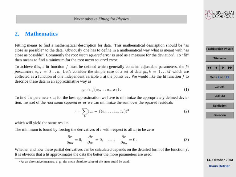
2. Mathematics

Fitting means to find a mathematical description for data. This mathematical description should be “asclose as possible” to the data. Obviously one has to define in a mathematical way what is meant with “asclose as possible”. Commonly theroot mean squared erroris used as a measure for the deviation2. To “fit”then means to find a minimum for theroot mean squared error.

To achieve this, a fit functionf must be defined which generally contains adjustable parameters, thefitparametersai, i = 0 . . . n. Let’s consider the simple case of a set of datayk, k = 1 . . .M which arecollected as a function of one independent variablex at the pointsxk. We would like the fit functionf todescribe these data in an approximative way as

yk ≈ f(a0, . . . an, xk) . (1)

To find the parametersai for the best approximation we have to minimize the appropriately defined devia-tion. Instead of theroot mean squared errorwe can minimize the sum over the squared residuals

r =∑

k

(yk − f(a0, . . . an, xk))2 (2)

which will yield the same results.

The minimum is found by forcing the derivatives ofr with respect to allai to be zero

∂r

∂a0= 0,

∂r

∂a1= 0, . . . ,

∂r

∂an= 0 . (3)

Whether and how these partial derivatives can be calculated depends on the detailed form of the functionf .It is obvious that a fit approximates the data the better the more parameters are used.

2As an alternative measure, e. g., the mean absolute value of the error could be used.

Fachbereich Physik

Titelseite

JJ J I II

Seite 3 von 22

Zuruck

Vollbild

Schließen

Beenden

14. Oktober 2003

Klaus Betzler

Degrees of Freedom: For a fit often a quantitydegrees of freedomis defined which is the differencebetween the number of the data points and the number of the parameters

df = M − (n + 1) . (4)

A positive value fordf would be wise.

Residuals: Theresidualsare the differences between data values and corresponding calculated fit data.

Norm of Residuals: The norm of a mathematical object is a quantity that – taken in the right sense –describes the length, size or extent of this object. Mathematically more precisely, usually theL2-norm ismeant. Given a vectorz

z =

z1

z2

...zn

(5)

the L2-norm is defined as||z||2 =

(|z1|2 + |z2|2 + . . . + |zn|2

)1/2. (6)

(For theLj-norm the ‘2’ in all exponents (2 and 1/2) must be replaced by the respective numberj. Alsocommonly used areL1 andL∞.)

Thenorm of residualsis thus the square root of ther defined in Eq.2. It is often used as a measure for thegoodness of fitwhen comparing different fits.

3. Polynomial Fits

The simplest sort of fit functions are polynomials

f(a0, . . . an, xk) = a0 + a1xk + . . . + anxnk . (7)

Fachbereich Physik

Titelseite

JJ J I II

Seite 4 von 22

Zuruck

Vollbild

Schließen

Beenden

14. Oktober 2003

Klaus Betzler

The sum of the squared residuals is

r =∑

k

(yk − a0 + a1xk + . . . + anxnk )2 , (8)

their partial derivative with respect toai

∂r

∂ai=

∑k

[2(yk − a0 + a1xk + . . . + anxn

k )xik

] != 0 (x0

k = 1) . (9)

Eq. 9 is a system ofn + 1 linear equations for then + 1 variable parametersai. It may be solved bystandard solution schemes for linear equations. Generally there is one unique solution, no approximativeoptimization procedures are necessary. Even more – when applied – optimization procedures may lead toerroneous results.

MATLAB: In MATLAB a polynomial fit can be directly performed in the figure window. Click onTools

andBasic Fitting and you can select polynomial orders. The results of the fit – parameters and the norm ofthe residuals – can be transferred to the workspace for further usage.

For doing it in a functional form, MATLAB provides the functionpolyfit . In the simplest form, youcall it for your data vectorsx andy through

P = polyfit(x,y,n);

for the polynomial ordern. Except the parameter vectorP , polyfit can also provide an additionalstructureS with more information, then you have to call it as

[P,S] = polyfit(x,y,n);

(more details in theHelp).

Fachbereich Physik

Titelseite

JJ J I II

Seite 5 von 22

Zuruck

Vollbild

Schließen

Beenden

14. Oktober 2003

Klaus Betzler

The corresponding values for the fit curve can be calculate through the functionpolyval . For drawingthe fit curve, it is useful to provide a vectorX with narrower spacing in order to get a smooth curve

X = linspace(min(x),max(x),500);Y = polyval(P,X); % values for fit curveh1 = plot(X,Y,’k’,...); % draw fit curvehold on;h2 = plot(x,y,’ko’,...); % draw datahold off;

The function polyval can use the additional informationS from polyfit to provide error estimates(see theHelp for more).

4. Parameter-Linear Fits

Similar to polynomial fits are so-calledparameter-linearfits, i. e. fits to an arbitrary function with the onlyrestriction that this function is linear in the fit parameters. Such a function can be written as a sum ofsimpler functions

f(a0, . . . an, xk) = a0 + a1f1(xk) + a2f2(xk) + . . . + anfn(xk) . (10)

Obviously polynomial fits are a special case of parameter-linear fits when you definefn(xk) = xnk .

Again one can calculate the sum of the squared residuals

r =∑

k

(yk − a0 + a1f1(xk) + . . . + anfn(xk))2 , (11)

and their partial derivative with respect toai

∂r

∂ai=

∑k

[2(yk − a0 + a1f1(xk) + . . . + anfn(xk))fi(xk)]!= 0 . (12)

And again we have to solve this system of linear equations which now is a little bit more complicated.

Fachbereich Physik

Titelseite

JJ J I II

Seite 6 von 22

Zuruck

Vollbild

Schließen

Beenden

14. Oktober 2003

Klaus Betzler

MATLAB: There is no dedicated fit function for this sort of parameter-linear fits in MATLAB. However,MATLAB knows how to solve a system of linear equations. Given such a system of linear equations

Az = b (13)

whereA is the matrix of the coefficients,z is the vector of the variables andb is the right hand side vectorof the equations, MATLAB solves this system using the functionmldivide (matrix left divide). Thisfunction can be abbreviated by ‘\’. The solution vector then is

z = mldivide(A,b);

or simpler

z = A\b; .

As can be seen in Eq.12, all these wicked productsfj(xk)fi(xk) have to be calculated and summed overkto get the coefficients of the matrixA for MATLAB. This can be written as a matrix product of 2 rectangular-shaped matrices. But MATLAB can help you to avoid all these formal calculations. The functionality ofmldivide has been extended to non-square matricesA. If A is rectangular, the problem is solved in a“least squares sense”, as MATLAB states. That’s exactly what one needs for fitting. We have to solve theset ofk equations (over-determined system of linear equations forai)

f(a0, . . . , an, xk) = y(k) (14)

in a least squares sense for the variablesai.

Written as matrices and vectors3

Fa = y with F =

1 f1(x1) · · · fn(x1)1 f1(x2) · · · fn(x2)...

......

...1 f1(xM ) · · · fn(xM )

(15)

3The parametera0 and the column of 1 s in the matrixF is only included here to show the formal correspondence with thepolynomial case. Usually it is omitted.

Fachbereich Physik

Titelseite

JJ J I II

Seite 7 von 22

Zuruck

Vollbild

Schließen

Beenden

14. Oktober 2003

Klaus Betzler

and solved by MATLAB as

a = mldivide(F,y); or a = F\y; .

A simple example is shown in Fig.1, a sinusoidal data set is to be approximated. Suppose you want toknow amplitude and phase, the data then are to be fitted by the function

y = A · sin(x + φ) (16)

with the two fit parametersA andφ. This fit function can be easily rewritten to the parameter-linear one

y = a1 sin(x) + a2 cos(x) (17)

which then is solved.

The data are provided by

X = linspace(0,20,100);Y = 1.9*sin(X+1.3*pi); .

Fitting is then a rather short sequence in the script:

F1 = sin(X);F2 = cos(X);F = [F1’,F2’];a = F\Y’; .

Using the fit parametersa, the relevant objects may be calculated

Yfit = F*a;amplitude = norm(a);phase = atan2(a(2),a(1));

Fachbereich Physik

Titelseite

JJ J I II

Seite 8 von 22

Zuruck

Vollbild

Schließen

Beenden

14. Oktober 2003

Klaus Betzler

the largest part of the script is wasted for plotting and formatting the plotgray = 0.7*[1,1,1];plot(X,F1,X,F2,’Color’,gray,’Linewidth’,2);hold on;plot(X,Yfit,’k’,’Linewidth’,2);plot(X,Y,’ko’,’Linewidth’,2,’Markerfacecolor’,’w’);hold off;set(gca,’Linewidth’,1.5);set(gca,’Fontunits’,’normalized’,’Fontsize’,0.06); .

5. Arbitrary Fit Functions

The two classes of fits described in the preceding sections are mathematically well determined. One can findexact unique solutions for the fit parameters4. Therefore one should use polynomial or parameter-linear fitswherever appropriate. Sometimes more complicated fit problems can be transformed to parameter-linearfits. If this is not possible, one has to use arbitrary fit functions which are no longer linear in the fitparameters.

These generalized fit problems have to be solved using optimization algorithms. The function to be opti-mized (i. e. minimized) is usually the sum of the squared residuals. One thus has to find the minimum ofan arbitrary, in general multidimensional function. The variable space of this multidimensional functionis defined by the fit parameters. One key issue in all such optimization problems is that there is usuallyno unique and exact way to find the solution. Approximative algorithms have to be applied. And there ispractically no simple way to check whether the algorithm has found the global (absolute) minimum or onlya local (relative) one.

4Problems may occur numerically when the system of linear equations is what you callbadly conditioned. But that’s a knownproblem in Linear Algebra and we will not deal with it at this point.

Fachbereich Physik

Titelseite

JJ J I II

Seite 9 von 22

Zuruck

Vollbild

Schließen

Beenden

14. Oktober 2003

Klaus Betzler

0 5 10 15 20−2

−1.5

−1

−0.5

0

0.5

1

1.5

2

Figure 1: Parameter-linear fit in MATLAB. Dots indicate the original data, gray lines are the two basefunctions, sine and cosine, and the black line represents the fit result (see text for details).

MATLAB: To search for the minimum of an arbitrary function, MATLAB provides the functionfminsearch .To use it, you have to write an additional short function calculating the value of the function to be mini-mized. If you would want, e. g., to fit a Lorentziany = a1/((x−a2)2 +a3) to a data setXi, Yi, you shoulddefine in MATLAB a function resulting in the sum of the squared residuals

function d = devsum(a)global X Yd = sum((Y - a(1)./((X-a(2)).ˆ2+a(3))).ˆ2); .

Fachbereich Physik

Titelseite

JJ J I II

Seite 10 von 22

Zuruck

Vollbild

Schließen

Beenden

14. Oktober 2003

Klaus Betzler

This function is then used in a call tofminsearch as the first parametera3 = ((max(X)-min(X))/10)ˆ2;a2 = (max(X)+min(X))/2;a1 = max(Y)*a3;a0 = [a1,a2,a3];afinal = fminsearch(@devsum,a0); .

The start values for the parameters (a1, a2, a3) could of course be chosen in a better way when the data setis known. An example for the fit with a Lorentzian is shown in Fig.2, the data set there was defined by

X = linspace(0,100,200);Y = 20./((X-30).ˆ2+20)+0.08*randn(size(X)); .

The function fminsearch can be tuned by additional options, one can demand a certain accuracy,restrict the number of optimization steps etc. For a detailed description consultHelp.

6. Weighted Fit

Up to this point we have assumed that all members of the data set underlying the fit are equal in theirreliability. If this is not the case, one should rate the different members with different weights where theweights should be a measure for the reliability. Introducing such weights, not the sum over the squaredresiduals is to be minimized, instead the sum over the squaredweightedresiduals has to be taken. Insteadof Eq.2 you should use

r =∑

k

(wk(yk − f(a0, . . . an, xk)))2 (18)

wherewk are the weights of the data pointsk.

Fachbereich Physik

Titelseite

JJ J I II

Seite 11 von 22

Zuruck

Vollbild

Schließen

Beenden

14. Oktober 2003

Klaus Betzler

0 20 40 60 80 100−0.2

0

0.2

0.4

0.6

0.8

1

1.2

Figure 2: Fitting in MATLAB with fminsearch . Dots indicate the original data, dashed line is thestarting Lorentzian, full line the fit result (see text for details).

MATLAB: To implement this in MATLAB is straightforward for the parameter-linear and the arbitrary-function fits. You can include it directly in your script. If you want to use the MATLAB functionpolyfit ,it has to be adapted by a few additional lines to allow for weighted fits.

You load the function into the MATLAB editor byedit polyfit.m and save it to your workingdirectory using a different name (e. g.wpolyfit ). The vector of the weightsw goes as an additionalparameter into the parameter list

function [p,S,mu] = wpolyfit(x,y,n,w) .

Fachbereich Physik

Titelseite

JJ J I II

Seite 12 von 22

Zuruck

Vollbild

Schließen

Beenden

14. Oktober 2003

Klaus Betzler

The values ofy and the Vandermonde matrixV have to be multiplied by the weights before solving theleast squares problem. This is done by some additional lines

w = w(:);y = y.*w;for j = 1:n+1

V(:,j) = w.*V(:,j);end .

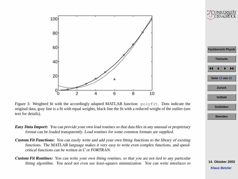
Fig. 3 shows the application of such a weighted fit on a set of data with an obvious outlier. The gray curverepresents an equally weighted polynomial fit, the black curve a fit where the outlier was given a weightfactor of 0.1, all other data a weight of 1.

Removal of outliers can be one application of weighted fits, taking into account different experimental errorsanother one. Given dataY with errorsDY , as weights the reciprocal errors can be used (w = 1./DY inMATLAB).

Before fitting data you should always analyze what exactly you want to get. An interpolation formula?Features like peak positions in a measured spectrum? The parameters of a physical model? The fitfunctions you provide will usually depend on this. MATLAB can only deliver the tools for the solution.

Appendix I:. Mfit – A Fitting Environment

Several people have developed a user interface for doing fits in MATLAB. They characterize it as follows:

Mfit is an application for interactive non-linear fitting and data analysis that runs under MATLAB (version4.2 or later). The primary aim of Mfit is to provide a fast, easy, flexible, and powerful way of fitting arbitrarymodel functions to two-dimensional (ie. x-y) data.

Easy Use: Mfit provides an attractive and easy to use point-and-click interface. Most operations (includingguessing starting parameters for fits) can be performed via the mouse.

Fachbereich Physik

Titelseite

JJ J I II

Seite 13 von 22

Zuruck

Vollbild

Schließen

Beenden

14. Oktober 2003

Klaus Betzler

0 2 4 6 8 100

20

40

60

80

100

Figure 3: Weighted fit with the accordingly adapted MATLAB functionpolyfit . Dots indicate theoriginal data, gray line is a fit with equal weights, black line the fit with a reduced weight of the outlier (seetext for details).

Easy Data Import: You can provide your own load routines so that data files in any unusual or proprietaryformat can be loaded transparently. Load routines for some common formats are supplied.

Custom Fit Functions: You can easily write and add your own fitting functions to the library of existingfunctions. The MATLAB language makes it very easy to write even complex functions, and speed-critical functions can be written in C or FORTRAN.

Custom Fit Routines: You can write your own fitting routines, so that you are not tied to any particularfitting algorithm. You need not even use least-squares minimization. You can write interfaces to

Fachbereich Physik

Titelseite

JJ J I II

Seite 14 von 22

Zuruck

Vollbild

Schließen

Beenden

14. Oktober 2003

Klaus Betzler

popular minimization routines such as MINUIT.

Easy Automation: Repetitive fitting operations can be automated using a simple batch language.

Portable: Mfit is written entirely in the MATLAB language, and so should run on any operating system towhich MATLAB has been ported without modification (tested under HP-UX, VMS, Sun OS, and allMS Windows so far.).

Mfit is public domainsoftware and can be downloaded from

http://www.ill.fr/tas/matlab/doc/mfit4/.

Appendix II:. Common Pitfalls

When you are fitting data you should carefully reflect on what you are doing. Many interesting pitfalls arewaiting in this field, some typical we should consider here.

A. The Noisy Zero

In many measurements in physics you measure intensities. And most measurements are noisy. Whathappens if you havezerointensity together with some amount of noise?

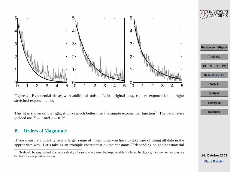
We consider the measurement of the exponential decay of a signal (e. g. the time dependance of the lumi-nescence after a pulsed laser excitation of some material). In the left sketch of Fig.4 the ideal exponentialdecay signal (I = A exp(−t/T ), T = 1 in the x-axis units) is shown (thick line) and some noise is added(thin line). If we try to fit the noisy signal with an exponential function, we get the result shown in thecenter. The exponential function fits the signal more or less, yet the time constant yielded is nowT = 1.42.To get a better fit, one could try a so-calledstretched-exponentialfunction (also known as Kohlrausch-Williams-Watts law)

I = A exp(−(t/T )q) with 0 < q ≤ 1 . (19)

Fachbereich Physik

Titelseite

JJ J I II

Seite 15 von 22

Zuruck

Vollbild

Schließen

Beenden

14. Oktober 2003

Klaus Betzler

0 1 2 3 4 50

1

2

3

4

5

0 1 2 3 4 50

1

2

3

4

5

0 1 2 3 4 50

1

2

3

4

5

Figure 4: Exponential decay with additional noise. Left: original data, center: exponential fit, right:stretched-exponential fit.

This fit is shown on the right, it looks much better than the simple exponential function5. The parametersyielded areT = 1 andq = 0.72.

B. Orders of Magnitude

If you measure a quantity over a larger range of magnitudes you have to take care of rating all data in theappropriate way. Let’s take as an example characteristic time constantsT depending on another material

5It should be emphasized that in practically all cases, where stretched exponentials are found in physics, they arenot due to noisebut have a clear physical reason.

Fachbereich Physik

Titelseite

JJ J I II

Seite 16 von 22

Zuruck

Vollbild

Schließen

Beenden

14. Oktober 2003

Klaus Betzler

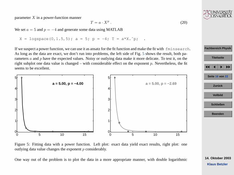
parameterX in a power-function mannerT = a ·Xp . (20)

We seta = 5 andp = −4 and generate some data using MATLAB

X = logspace(0,1.5,5); a = 5; p = -4; T = a*X.ˆp; .

If we suspect a power function, we can use it as ansatz for the fit function and make the fit withfminsearch .As long as the data are exact, we don’t run into problems, the left side of Fig.5 shows the result, both pa-rametersa andp have the expected values. Noisy or outlying data make it more delicate. To test it, on theright subplot one data value is changed – with considerable effect on the exponentp. Nevertheless, the fitseems to be excellent.

a = 5.00, p = −4.00

0 5 10 150

1

2

3

4

5

a = 5.00, p = −2.69

0 5 10 150

1

2

3

4

5

Figure 5: Fitting data with a power function. Left plot: exact data yield exact results, right plot: oneoutlying data value changes the exponentp considerably.

One way out of the problem is to plot the data in a more appropriate manner, with double logarithmic

Fachbereich Physik

Titelseite

JJ J I II

Seite 17 von 22

Zuruck

Vollbild

Schließen

Beenden

14. Oktober 2003

Klaus Betzler

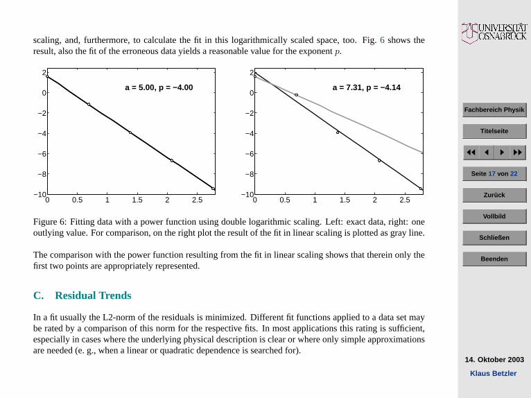
scaling, and, furthermore, to calculate the fit in this logarithmically scaled space, too. Fig.6 shows theresult, also the fit of the erroneous data yields a reasonable value for the exponentp.

a = 5.00, p = −4.00

0 0.5 1 1.5 2 2.5−10

−8

−6

−4

−2

0

2

a = 7.31, p = −4.14

0 0.5 1 1.5 2 2.5−10

−8

−6

−4

−2

0

2

Figure 6: Fitting data with a power function using double logarithmic scaling. Left: exact data, right: oneoutlying value. For comparison, on the right plot the result of the fit in linear scaling is plotted as gray line.

The comparison with the power function resulting from the fit in linear scaling shows that therein only thefirst two points are appropriately represented.

C. Residual Trends

In a fit usually the L2-norm of the residuals is minimized. Different fit functions applied to a data set maybe rated by a comparison of this norm for the respective fits. In most applications this rating is sufficient,especially in cases where the underlying physical description is clear or where only simple approximationsare needed (e. g., when a linear or quadratic dependence is searched for).

Fachbereich Physik

Titelseite

JJ J I II

Seite 18 von 22

Zuruck

Vollbild

Schließen

Beenden

14. Oktober 2003

Klaus Betzler

Complications may occur in cases where you are not sure what fit function to use.Table lookup6 applica-tions are the typical scenarios. In such cases it is useful not only to rate the norm of the residuals but alsoto plot the residuals to get a graphical impression of typical trends.

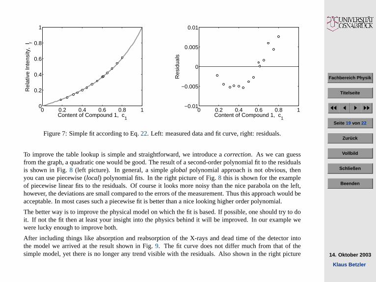
We look at an example. In unknown mixtures of two compounds the content of each is to be measuredwith high accuracy. The two compounds are represented by the respective count rates,N1 andN2, in twodistinct spectral lines of an X-ray fluorescence spectrum. To get rid of geometry effects, fluctuations in theexciting radiation etc., a normalized relative intensity ratioIr is calculated

Ir =N1

N1 + N2(21)

which is a measure for the content of compound 1 in the mixture,c1. Unfortunately there is no lineardependance betweenc1 andIr.

To get alookup tablefor the measurement of the unknown samples, known standard mixtures are measuredwith high accuracy. It is assumed for the first that the deviation from the linear dependance betweenc1 andR can be referred to different quantum efficiencies for the two spectral lines. This would yield

Ir =q1c1

q1c1 + q2c2=

c1

c1 + Qc2(22)

with the quantum efficienciesqi and their ratioQ (for Q = 1 we would have linearity asc1+c2 = 1). Fig.7shows on the left the intensity ratiosIr as a function of the amount of compound 1,c1, for the standardsmeasured (dots) together with the fit according to Eq.22with Q as fit parameter (gray line).

Obviously an excellent fit we could be content with. However, we always want to know, how good wereally are. Therefore we plot the residuals (right of Fig.7) – and – see that we haven’t got the whole truth.

How to deal with ? It’s table lookupand it’s physics. So we can choose: improve the table lookup algorithmor improve the physics.

6Table lookupis quite often used in physics to relate properties depending on each other with no or no simple functional relation.Think of measuring temperature using a thermocouple: You measure the voltage and look into a table where the voltages are referredto temperatures. Usually you don’t find the exact voltage you have measured. If your table is accurate enough (as usual for athermocouple), you can interpolate to get the temperature. If the table data are noisy, you should apply a fitting strategy.

Fachbereich Physik

Titelseite

JJ J I II

Seite 19 von 22

Zuruck

Vollbild

Schließen

Beenden

14. Oktober 2003

Klaus Betzler

0 0.2 0.4 0.6 0.8 10

0.2

0.4

0.6

0.8

1

Content of Compound 1, c1

Rel

ativ

e In

tens

ity,

I r

0 0.2 0.4 0.6 0.8 1−0.01

−0.005

0

0.005

0.01

Content of Compound 1, c1

Res

idua

ls

Figure 7: Simple fit according to Eq.22. Left: measured data and fit curve, right: residuals.

To improve the table lookup is simple and straightforward, we introduce acorrection. As we can guessfrom the graph, a quadratic one would be good. The result of a second-order polynomial fit to the residualsis shown in Fig.8 (left picture). In general, a simpleglobal polynomial approach is not obvious, thenyou can use piecewise (local) polynomial fits. In the right picture of Fig.8 this is shown for the exampleof piecewise linear fits to the residuals. Of course it looks more noisy than the nice parabola on the left,however, the deviations are small compared to the errors of the measurement. Thus this approach would beacceptable. In most cases such a piecewise fit is better than a nice looking higher order polynomial.

The better way is to improve the physical model on which the fit is based. If possible, one should try to doit. If not the fit then at least your insight into the physics behind it will be improved. In our example wewere lucky enough to improve both.

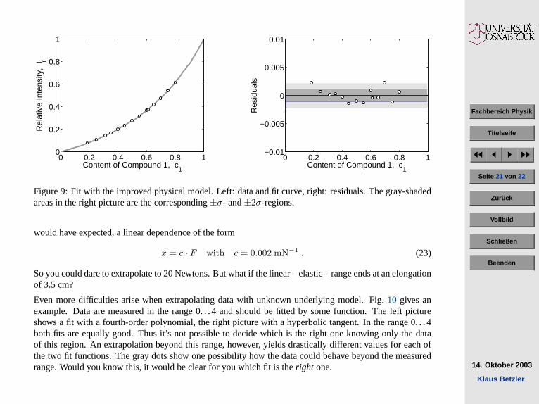
After including things like absorption and reabsorption of the X-rays and dead time of the detector intothe model we arrived at the result shown in Fig.9. The fit curve does not differ much from that of thesimple model, yet there is no longer any trend visible with the residuals. Also shown in the right picture

Fachbereich Physik

Titelseite

JJ J I II

Seite 20 von 22

Zuruck

Vollbild

Schließen

Beenden

14. Oktober 2003

Klaus Betzler

0 0.2 0.4 0.6 0.8 1−0.01

−0.005

0

0.005

0.01

Content of Compound 1, c1

Res

idua

ls

0 0.2 0.4 0.6 0.8 1−0.01

−0.005

0

0.005

0.01

Content of Compound 1, c1

Res

idua

ls

Figure 8: Left: Fit to the residuals using a second-order polynomial. Right: Piecewise linear fit to theresiduals. Two fit examples are shown. The areas where the data are taken for the respective linear fitsare shaded in gray, the fit lines are dashed. The resulting fit points are shown black-filled. The dark graypiecewise linear curve is the complete result of the fit procedure.

are the error margins (standard deviations)±σ and±2σ of the data which help to rate the reliability of themeasurements (if more than 68 % of the data are within the±σ-region, there might be something wrong).

D. Extrapolation

To rate the reliability of a fit, it is useful to have some data around. But what if you need values outsidethe range measured data? You can try toextrapolate. That might be unproblematic as long as there is somevalid physical concept around. Think of a spring in its elastic range. With a forceF of 5 Newtons youmeasure an elongationx of 1 cm, with 10 Newtons then 2 cm, with 15 Newtons 3 cm. Obviously, as you

Fachbereich Physik

Titelseite

JJ J I II

Seite 21 von 22

Zuruck

Vollbild

Schließen

Beenden

14. Oktober 2003

Klaus Betzler

0 0.2 0.4 0.6 0.8 10

0.2

0.4

0.6

0.8

1

Content of Compound 1, c1

Rel

ativ

e In

tens

ity,

I r

0 0.2 0.4 0.6 0.8 1−0.01

−0.005

0

0.005

0.01

Content of Compound 1, c1

Res

idua

ls

Figure 9: Fit with the improved physical model. Left: data and fit curve, right: residuals. The gray-shadedareas in the right picture are the corresponding±σ- and±2σ-regions.

would have expected, a linear dependence of the form

x = c · F with c = 0.002 mN−1 . (23)

So you could dare to extrapolate to 20 Newtons. But what if the linear – elastic – range ends at an elongationof 3.5 cm?

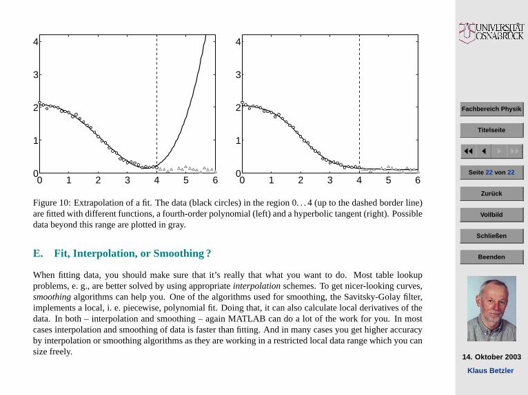
Even more difficulties arise when extrapolating data with unknown underlying model. Fig.10 gives anexample. Data are measured in the range 0. . . 4 and should be fitted by some function. The left pictureshows a fit with a fourth-order polynomial, the right picture with a hyperbolic tangent. In the range 0. . . 4both fits are equally good. Thus it’s not possible to decide which is the right one knowing only the dataof this region. An extrapolation beyond this range, however, yields drastically different values for each ofthe two fit functions. The gray dots show one possibility how the data could behave beyond the measuredrange. Would you know this, it would be clear for you which fit is theright one.

Fachbereich Physik

Titelseite

JJ J I II

Seite 22 von 22

Zuruck

Vollbild

Schließen

Beenden

14. Oktober 2003

Klaus Betzler

0 1 2 3 4 5 60

1

2

3

4

0 1 2 3 4 5 60

1

2

3

4

Figure 10: Extrapolation of a fit. The data (black circles) in the region 0. . . 4 (up to the dashed border line)are fitted with different functions, a fourth-order polynomial (left) and a hyperbolic tangent (right). Possibledata beyond this range are plotted in gray.

E. Fit, Interpolation, or Smoothing ?

When fitting data, you should make sure that it’s really that what you want to do. Most table lookupproblems, e. g., are better solved by using appropriateinterpolationschemes. To get nicer-looking curves,smoothingalgorithms can help you. One of the algorithms used for smoothing, the Savitsky-Golay filter,implements a local, i. e. piecewise, polynomial fit. Doing that, it can also calculate local derivatives of thedata. In both – interpolation and smoothing – again MATLAB can do a lot of the work for you. In mostcases interpolation and smoothing of data is faster than fitting. And in many cases you get higher accuracyby interpolation or smoothing algorithms as they are working in a restricted local data range which you cansize freely.