Embed Size (px)
Citation preview

Simple Challenges Longitudinal Non-nested GLMMs Theory
Fitting Mixed-Effects ModelsUsing the lme4 Package in R
Douglas Bates
University of Wisconsin - Madisonand R Development Core Team
International Meeting of the Psychometric SocietyJune 29, 2008
Simple Challenges Longitudinal Non-nested GLMMs Theory
Outline
Organizing and plotting data; simple, scalar random effects
Mixed-modeling challenges
Models for longitudinal data
Unbalanced, non-nested data sets
Generalized linear mixed models
Evaluating the log-likelihood
Simple Challenges Longitudinal Non-nested GLMMs Theory
Outline
Organizing and plotting data; simple, scalar random effects
Mixed-modeling challenges
Models for longitudinal data
Unbalanced, non-nested data sets
Generalized linear mixed models
Evaluating the log-likelihood
Simple Challenges Longitudinal Non-nested GLMMs Theory
Outline
Organizing and plotting data; simple, scalar random effects
Mixed-modeling challenges
Models for longitudinal data
Unbalanced, non-nested data sets
Generalized linear mixed models
Evaluating the log-likelihood
Simple Challenges Longitudinal Non-nested GLMMs Theory
Outline
Organizing and plotting data; simple, scalar random effects
Mixed-modeling challenges
Models for longitudinal data
Unbalanced, non-nested data sets
Generalized linear mixed models
Evaluating the log-likelihood
Simple Challenges Longitudinal Non-nested GLMMs Theory
Outline
Organizing and plotting data; simple, scalar random effects
Mixed-modeling challenges
Models for longitudinal data
Unbalanced, non-nested data sets
Generalized linear mixed models
Evaluating the log-likelihood
Simple Challenges Longitudinal Non-nested GLMMs Theory
Outline
Organizing and plotting data; simple, scalar random effects
Mixed-modeling challenges
Models for longitudinal data
Unbalanced, non-nested data sets
Generalized linear mixed models
Evaluating the log-likelihood

Simple Challenges Longitudinal Non-nested GLMMs Theory
Web sites associated with the workshop
www.stat.wisc.edu/∼bates/IMPS2008 Materials for the course
www.r-project.org Main web site for the R Project
cran.r-project.org Comprehensive R Archive Network primary site
cran.us.r-project.org Main U.S. mirror for CRAN
cran.R-project.org/web/views/Psychometrics.html Psychometricstask view within CRAN
R-forge.R-project.org R-Forge, development site for many public Rpackages
lme4.R-forge.R-project.org development site for the lme4 package
Simple Challenges Longitudinal Non-nested GLMMs Theory
Organizing data in R
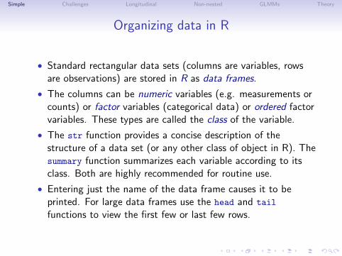
• Standard rectangular data sets (columns are variables, rowsare observations) are stored in R as data frames.
• The columns can be numeric variables (e.g. measurements orcounts) or factor variables (categorical data) or ordered factorvariables. These types are called the class of the variable.
• The str function provides a concise description of thestructure of a data set (or any other class of object in R). Thesummary function summarizes each variable according to itsclass. Both are highly recommended for routine use.
• Entering just the name of the data frame causes it to beprinted. For large data frames use the head and tail
functions to view the first few or last few rows.

Simple Challenges Longitudinal Non-nested GLMMs Theory
R packages
• Packages incorporate functions, data and documentation.
• You can produce packages for private or in-house use or youcan contribute your package to the Comprehensive R ArchiveNetwork (CRAN), http://cran.us.R-project.org
• We will be using the lme4 package from CRAN. Install it fromthe Packages menu item or with> install.packages("lme4")
• You only need to install a package once. If a new versionbecomes available you can update (see the menu item).
• To use a package in an R session you attach it using> require(lme4)
or> library(lme4)
(This usage causes widespread confusion of the terms“package” and “library”.)
Simple Challenges Longitudinal Non-nested GLMMs Theory
Accessing documentation
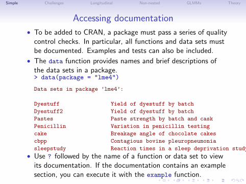
• To be added to CRAN, a package must pass a series of qualitycontrol checks. In particular, all functions and data sets mustbe documented. Examples and tests can also be included.
• The data function provides names and brief descriptions ofthe data sets in a package.> data(package = "lme4")
Data sets in package ’lme4’:
Dyestuff Yield of dyestuff by batch
Dyestuff2 Yield of dyestuff by batch
Pastes Paste strength by batch and cask
Penicillin Variation in penicillin testing
cake Breakage angle of chocolate cakes
cbpp Contagious bovine pleuropneumonia
sleepstudy Reaction times in a sleep deprivation study
• Use ? followed by the name of a function or data set to viewits documentation. If the documentation contains an examplesection, you can execute it with the example function.
Simple Challenges Longitudinal Non-nested GLMMs Theory
Lattice graphics
• One of the strengths of R is its graphics capabilities.
• There are several styles of graphics in R. The style inDeepayan Sarkar’s lattice package is well-suited to the type ofdata we will be discussing.
• I will not show every piece of code used to produce the datagraphics. The code is available in the script files for the slides(and sometimes in the example sections of the data set’sdocumentation).
• Deepayan’s book, Lattice: Multivariate Data Visualizationwith R (Springer, 2008) provides in-depth documentation andexplanations of lattice graphics.
• I also recommend Phil Spector’s book, Data Manipulationwith R (Springer, 2008).
Simple Challenges Longitudinal Non-nested GLMMs Theory
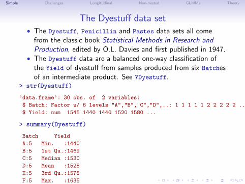
The Dyestuff data set• The Dyestuff, Penicillin and Pastes data sets all come
from the classic book Statistical Methods in Research andProduction, edited by O.L. Davies and first published in 1947.
• The Dyestuff data are a balanced one-way classification ofthe Yield of dyestuff from samples produced from six Batchesof an intermediate product. See ?Dyestuff.
> str(Dyestuff)
’data.frame’: 30 obs. of 2 variables:
$ Batch: Factor w/ 6 levels "A","B","C","D",..: 1 1 1 1 1 2 2 2 2 2 ...
$ Yield: num 1545 1440 1440 1520 1580 ...
> summary(Dyestuff)
Batch Yield
A:5 Min. :1440
B:5 1st Qu.:1469
C:5 Median :1530
D:5 Mean :1528
E:5 3rd Qu.:1575
F:5 Max. :1635
Simple Challenges Longitudinal Non-nested GLMMs Theory
The effect of the batches
• To emphasize that Batch is categorical, we use letters insteadof numbers to designate the levels.
• Because there is no inherent ordering of the levels of Batch,we will reorder the levels if, say, doing so can make a plotmore informative.
• The particular batches observed are just a selection of thepossible batches and are entirely used up during the course ofthe experiment.
• It is not particularly important to estimate and compare yieldsfrom these batches. Instead we wish to estimate thevariability in yields due to batch-to-batch variability.
• The Batch factor will be used in random-effects terms inmodels that we fit.
Simple Challenges Longitudinal Non-nested GLMMs Theory
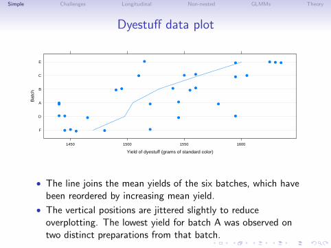
Dyestuff data plot
Yield of dyestuff (grams of standard color)
Bat
ch
F
D
A
B
C
E
1450 1500 1550 1600
●●● ● ●
●●●
●●
●● ●●
●
●● ●● ●
● ●●●●
●●
● ●●
• The line joins the mean yields of the six batches, which havebeen reordered by increasing mean yield.
• The vertical positions are jittered slightly to reduceoverplotting. The lowest yield for batch A was observed ontwo distinct preparations from that batch.
Simple Challenges Longitudinal Non-nested GLMMs Theory
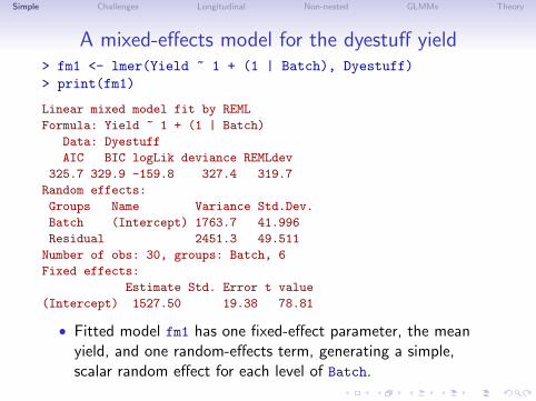
A mixed-effects model for the dyestuff yield> fm1 <- lmer(Yield ~ 1 + (1 | Batch), Dyestuff)> print(fm1)
Linear mixed model fit by REML
Formula: Yield ~ 1 + (1 | Batch)
Data: Dyestuff
AIC BIC logLik deviance REMLdev
325.7 329.9 -159.8 327.4 319.7
Random effects:
Groups Name Variance Std.Dev.
Batch (Intercept) 1763.7 41.996
Residual 2451.3 49.511
Number of obs: 30, groups: Batch, 6
Fixed effects:
Estimate Std. Error t value
(Intercept) 1527.50 19.38 78.81
• Fitted model fm1 has one fixed-effect parameter, the meanyield, and one random-effects term, generating a simple,scalar random effect for each level of Batch.
Simple Challenges Longitudinal Non-nested GLMMs Theory
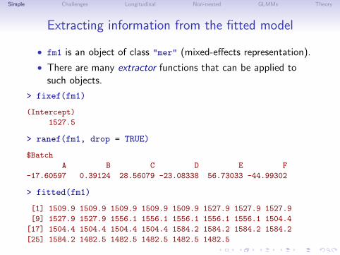
Extracting information from the fitted model
• fm1 is an object of class "mer" (mixed-effects representation).
• There are many extractor functions that can be applied tosuch objects.
> fixef(fm1)
(Intercept)
1527.5
> ranef(fm1, drop = TRUE)
$Batch
A B C D E F
-17.60597 0.39124 28.56079 -23.08338 56.73033 -44.99302
> fitted(fm1)
[1] 1509.9 1509.9 1509.9 1509.9 1509.9 1527.9 1527.9 1527.9
[9] 1527.9 1527.9 1556.1 1556.1 1556.1 1556.1 1556.1 1504.4
[17] 1504.4 1504.4 1504.4 1504.4 1584.2 1584.2 1584.2 1584.2
[25] 1584.2 1482.5 1482.5 1482.5 1482.5 1482.5
Simple Challenges Longitudinal Non-nested GLMMs Theory
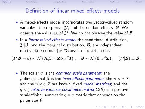
Definition of linear mixed-effects models
• A mixed-effects model incorporates two vector-valued randomvariables: the response, Y , and the random effects, B. Weobserve the value, y, of Y . We do not observe the value of B.
• In a linear mixed-effects model the conditional distribution,Y |B, and the marginal distribution, B, are independent,multivariate normal (or “Gaussian”) distributions,
(Y |B = b) ∼ N(Xβ + Zb, σ2I
), B ∼ N
(0, σ2Σ
), (Y |B) ⊥ B.
• The scalar σ is the common scale parameter; thep-dimensional β is the fixed-effects parameter; the n× p Xand the n× q Z are known, fixed model matrices; and theq × q relative variance-covariance matrix Σ(θ) is a positivesemidefinite, symmetric q × q matrix that depends on theparameter θ.
Simple Challenges Longitudinal Non-nested GLMMs Theory
Conditional modes of the random effects
• Technically we do not provide “estimates” of the randomeffects because they are not parameters.
• One answer to the question, “so what are those numbersanyway?” is that they are BLUPs (Best Linear UnbiasedPredictors) but that answer is not informative and the conceptdoes not generalize.
• A better answer is that those values are the conditionalmeans, E[B|Y = y], evaluated at the estimated parameters.Regrettably, we can only evaluate the conditional means forlinear mixed models.
• However, these values are also the conditional modes and thatconcept does generalize to other types of mixed models.
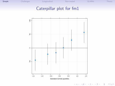
• For linear mixed models we can evaluate the conditionalstandard deviations of these random variables and plot aprediction interval. These intervals can be arranged in anormal probability plot, sometimes called a “caterpillar plot”.
Simple Challenges Longitudinal Non-nested GLMMs Theory
Caterpillar plot for fm1
Standard normal quantiles
−50
050
100
−1.5 −1.0 −0.5 0.0 0.5 1.0 1.5
●
●
●
●
●
●
Simple Challenges Longitudinal Non-nested GLMMs Theory
Mixed-effects model formulas
• In lmer the model is specified by the formula argument. As inmost R model-fitting functions, this is the first argument.
• The model formula consists of two expressions separated bythe ∼ symbol.
• The expression on the left, typically the name of a variable, isevaluated as the response.
• The right-hand side consists of one or more terms separatedby ‘+’ symbols.
• A random-effects term consists of two expressions separatedby the vertical bar, (‘|’), symbol (read as “given” or “by”).Typically, such terms are enclosed in parentheses.
• The expression on the right of the ‘|’ is evaluated as a factor,which we call the grouping factor for that term.
Simple Challenges Longitudinal Non-nested GLMMs Theory
Simple, scalar random-effects terms
• In a simple, scalar random-effects term, the expression on theleft of the ‘|’ is ‘1’. Such a term generates one random effect(i.e. a scalar) for each level of the grouping factor.
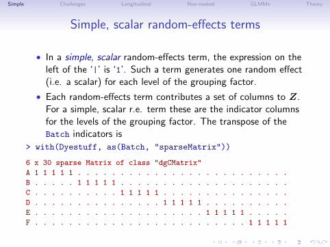
• Each random-effects term contributes a set of columns to Z.For a simple, scalar r.e. term these are the indicator columnsfor the levels of the grouping factor. The transpose of theBatch indicators is
> with(Dyestuff, as(Batch, "sparseMatrix"))
6 x 30 sparse Matrix of class "dgCMatrix"
A 1 1 1 1 1 . . . . . . . . . . . . . . . . . . . . . . . . .
B . . . . . 1 1 1 1 1 . . . . . . . . . . . . . . . . . . . .
C . . . . . . . . . . 1 1 1 1 1 . . . . . . . . . . . . . . .
D . . . . . . . . . . . . . . . 1 1 1 1 1 . . . . . . . . . .
E . . . . . . . . . . . . . . . . . . . . 1 1 1 1 1 . . . . .
F . . . . . . . . . . . . . . . . . . . . . . . . . 1 1 1 1 1
Simple Challenges Longitudinal Non-nested GLMMs Theory
Formulation of the marginal variance matrix
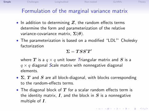
• In addition to determining Z, the random effects termsdetermine the form and parameterization of the relativevariance-covariance matrix, Σ(θ).
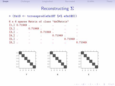
• The parameterization is based on a modified “LDL′” Choleskyfactorization
Σ = TSS′T ′
where T is a q × q unit lower Triangular matrix and S is aq × q diagonal Scale matrix with nonnegative diagonalelements.
• Σ, T and S are all block-diagonal, with blocks correspondingto the random-effects terms.
• The diagonal block of T for a scalar random effects term isthe identity matrix, I, and the block in S is a nonnegativemultiple of I.
Simple Challenges Longitudinal Non-nested GLMMs Theory
Verbose fitting, extracting T and S
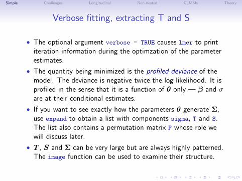
• The optional argument verbose = TRUE causes lmer to printiteration information during the optimzation of the parameterestimates.
• The quantity being minimized is the profiled deviance of themodel. The deviance is negative twice the log-likelihood. It isprofiled in the sense that it is a function of θ only — β and σare at their conditional estimates.
• If you want to see exactly how the parameters θ generate Σ,use expand to obtain a list with components sigma, T and S.The list also contains a permutation matrix P whose role wewill discuss later.
• T , S and Σ can be very large but are always highly patterned.The image function can be used to examine their structure.
Simple Challenges Longitudinal Non-nested GLMMs Theory
Obtain the verbose output for fitting fm1
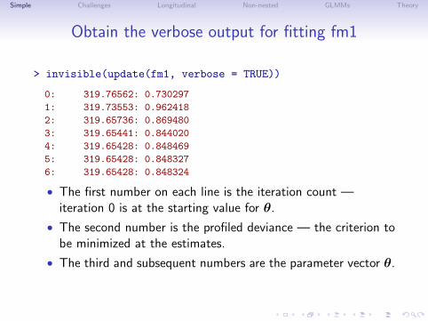
> invisible(update(fm1, verbose = TRUE))
0: 319.76562: 0.730297
1: 319.73553: 0.962418
2: 319.65736: 0.869480
3: 319.65441: 0.844020
4: 319.65428: 0.848469
5: 319.65428: 0.848327
6: 319.65428: 0.848324
• The first number on each line is the iteration count —iteration 0 is at the starting value for θ.
• The second number is the profiled deviance — the criterion tobe minimized at the estimates.
• The third and subsequent numbers are the parameter vector θ.
Simple Challenges Longitudinal Non-nested GLMMs Theory
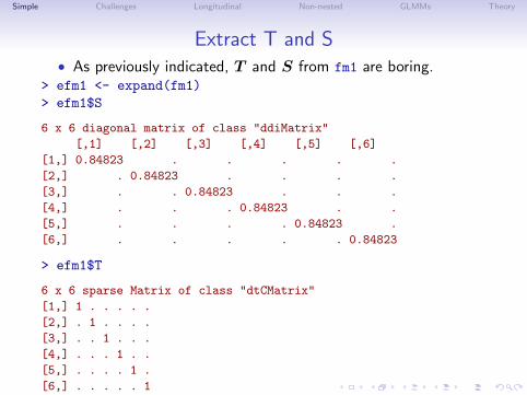
Extract T and S• As previously indicated, T and S from fm1 are boring.
> efm1 <- expand(fm1)> efm1$S
6 x 6 diagonal matrix of class "ddiMatrix"
[,1] [,2] [,3] [,4] [,5] [,6]
[1,] 0.84823 . . . . .
[2,] . 0.84823 . . . .
[3,] . . 0.84823 . . .
[4,] . . . 0.84823 . .
[5,] . . . . 0.84823 .
[6,] . . . . . 0.84823
> efm1$T
6 x 6 sparse Matrix of class "dtCMatrix"
[1,] 1 . . . . .
[2,] . 1 . . . .
[3,] . . 1 . . .
[4,] . . . 1 . .
[5,] . . . . 1 .
[6,] . . . . . 1
Simple Challenges Longitudinal Non-nested GLMMs Theory
Reconstructing Σ
> (fm1S <- tcrossprod(efm1$T %*% efm1$S))
6 x 6 sparse Matrix of class "dsCMatrix"
[1,] 0.71949 . . . . .
[2,] . 0.71949 . . . .
[3,] . . 0.71949 . . .
[4,] . . . 0.71949 . .
[5,] . . . . 0.71949 .
[6,] . . . . . 0.71949
T
1
2
3
4
5
6
1 2 3 4 5 6
S
1
2
3
4
5
6
1 2 3 4 5 6
ΣΣ
1
2
3
4
5
6
1 2 3 4 5 6
Simple Challenges Longitudinal Non-nested GLMMs Theory
REML estimates versus ML estimates
• The default parameter estimation criterion for linear mixedmodels is restricted (or “residual”) maximum likelihood(REML).
• Maximum likelihood (ML) estimates (sometimes called “fullmaximum likelihood”) can be requested by specifying REML =
FALSE in the call to lmer.
• Generally REML estimates of variance components arepreferred. ML estimates are known to be biased. AlthoughREML estimates are not guaranteed to be unbiased, they areusually less biased than ML estimates.
• Roughly the difference between REML and ML estimates ofvariance components is comparable to estimating σ2 in afixed-effects regression by SSR/(n− p) versus SSR/n, whereSSR is the residual sum of squares.
• For a balanced, one-way classification like the Dyestuff data,the REML and ML estimates of the fixed-effects are identical.
Simple Challenges Longitudinal Non-nested GLMMs Theory
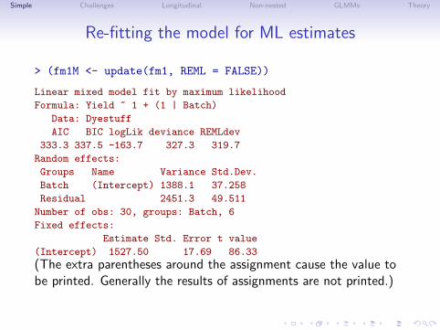
Re-fitting the model for ML estimates
> (fm1M <- update(fm1, REML = FALSE))
Linear mixed model fit by maximum likelihood
Formula: Yield ~ 1 + (1 | Batch)
Data: Dyestuff
AIC BIC logLik deviance REMLdev
333.3 337.5 -163.7 327.3 319.7
Random effects:
Groups Name Variance Std.Dev.
Batch (Intercept) 1388.1 37.258
Residual 2451.3 49.511
Number of obs: 30, groups: Batch, 6
Fixed effects:
Estimate Std. Error t value
(Intercept) 1527.50 17.69 86.33
(The extra parentheses around the assignment cause the value tobe printed. Generally the results of assignments are not printed.)
Simple Challenges Longitudinal Non-nested GLMMs Theory
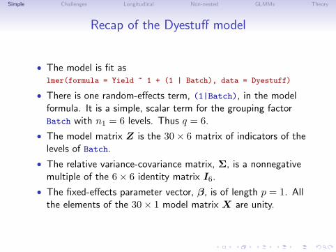
Recap of the Dyestuff model
• The model is fit aslmer(formula = Yield ~ 1 + (1 | Batch), data = Dyestuff)
• There is one random-effects term, (1|Batch), in the modelformula. It is a simple, scalar term for the grouping factorBatch with n1 = 6 levels. Thus q = 6.
• The model matrix Z is the 30× 6 matrix of indicators of thelevels of Batch.
• The relative variance-covariance matrix, Σ, is a nonnegativemultiple of the 6× 6 identity matrix I6.
• The fixed-effects parameter vector, β, is of length p = 1. Allthe elements of the 30× 1 model matrix X are unity.

Simple Challenges Longitudinal Non-nested GLMMs Theory
The Penicillin data (also check the ?Penicillin description)> str(Penicillin)
’data.frame’: 144 obs. of 3 variables:
$ diameter: num 27 23 26 23 23 21 27 23 26 23 ...
$ plate : Factor w/ 24 levels "a","b","c","d",..: 1 1 1 1 1 1 2 2 2 2 ...
$ sample : Factor w/ 6 levels "A","B","C","D",..: 1 2 3 4 5 6 1 2 3 4 ...
> xtabs(~sample + plate, Penicillin)
plate
sample a b c d e f g h i j k l m n o p q r s t u v w x
A 1 1 1 1 1 1 1 1 1 1 1 1 1 1 1 1 1 1 1 1 1 1 1 1
B 1 1 1 1 1 1 1 1 1 1 1 1 1 1 1 1 1 1 1 1 1 1 1 1
C 1 1 1 1 1 1 1 1 1 1 1 1 1 1 1 1 1 1 1 1 1 1 1 1
D 1 1 1 1 1 1 1 1 1 1 1 1 1 1 1 1 1 1 1 1 1 1 1 1
E 1 1 1 1 1 1 1 1 1 1 1 1 1 1 1 1 1 1 1 1 1 1 1 1
F 1 1 1 1 1 1 1 1 1 1 1 1 1 1 1 1 1 1 1 1 1 1 1 1
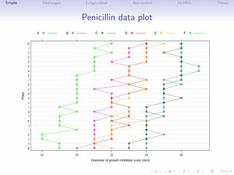
• These are measurements of the potency (measured by thediameter of a clear area on a Petri dish) of penicillin samplesin a balanced, unreplicated two-way crossed classification withthe test medium, plate.
Simple Challenges Longitudinal Non-nested GLMMs Theory
Penicillin data plot
Diameter of growth inhibition zone (mm)
Pla
te
g
s
x
u
i
j
w
f
q
r
v
e
p
c
d
l
n
a
b
h
k
o
t
m
18 20 22 24 26
●
●
●
●
●
●
●
●
●
●
●
●
●
●
●
●
●
●
●
●
●
●
●
●
●
●
●
●
●
●
●
●
●
●
●
●
●
●
●
●
●
●
●
●
●
●
●
●
●
●
●
●
●
●
●
●
●
●
●
●
●
●
●
●
●
●
●
●
●
●
●
●
●
●
●
●
●
●
●
●
●
●
●
●
●
●
●
●
●
●
●
●
●
●
●
●
●
●
●
●
●
●
●
●
●
●
●
●
●
●
●
●
●
●
●
●
●
●
●
●
●
●
●
●
●
●
●
●
●
●
●
●
●
●
●
●
●
●
●
●
●
●
●
●
A B C D E F● ● ● ● ● ●
Simple Challenges Longitudinal Non-nested GLMMs Theory
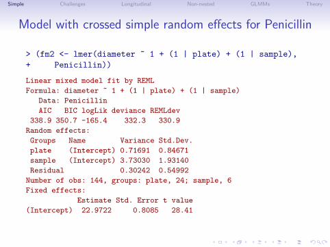
Model with crossed simple random effects for Penicillin
> (fm2 <- lmer(diameter ~ 1 + (1 | plate) + (1 | sample),+ Penicillin))
Linear mixed model fit by REML
Formula: diameter ~ 1 + (1 | plate) + (1 | sample)
Data: Penicillin
AIC BIC logLik deviance REMLdev
338.9 350.7 -165.4 332.3 330.9
Random effects:
Groups Name Variance Std.Dev.
plate (Intercept) 0.71691 0.84671
sample (Intercept) 3.73030 1.93140
Residual 0.30242 0.54992
Number of obs: 144, groups: plate, 24; sample, 6
Fixed effects:
Estimate Std. Error t value
(Intercept) 22.9722 0.8085 28.41
Simple Challenges Longitudinal Non-nested GLMMs Theory
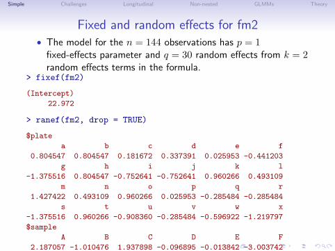
Fixed and random effects for fm2• The model for the n = 144 observations has p = 1
fixed-effects parameter and q = 30 random effects from k = 2random effects terms in the formula.
> fixef(fm2)
(Intercept)
22.972
> ranef(fm2, drop = TRUE)
$plate
a b c d e f
0.804547 0.804547 0.181672 0.337391 0.025953 -0.441203
g h i j k l
-1.375516 0.804547 -0.752641 -0.752641 0.960266 0.493109
m n o p q r
1.427422 0.493109 0.960266 0.025953 -0.285484 -0.285484
s t u v w x
-1.375516 0.960266 -0.908360 -0.285484 -0.596922 -1.219797
$sample
A B C D E F
2.187057 -1.010476 1.937898 -0.096895 -0.013842 -3.003742
Simple Challenges Longitudinal Non-nested GLMMs Theory
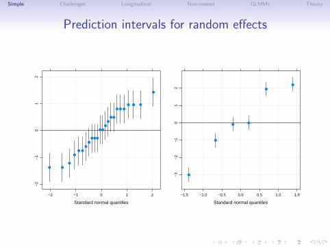
Prediction intervals for random effects
Standard normal quantiles
−2
−1
01
2
−2 −1 0 1 2
● ●
●
●
● ●
●
●
● ● ●
● ●
●
●
● ●
● ● ●
● ● ●
●
Standard normal quantiles
−3
−2
−1
01
2
−1.5 −1.0 −0.5 0.0 0.5 1.0 1.5
●
●
●●
●
●
Simple Challenges Longitudinal Non-nested GLMMs Theory
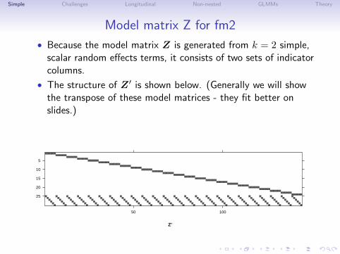
Model matrix Z for fm2
• Because the model matrix Z is generated from k = 2 simple,scalar random effects terms, it consists of two sets of indicatorcolumns.
• The structure of Z ′ is shown below. (Generally we will showthe transpose of these model matrices - they fit better onslides.)
Z'
5
10
15
20
25
50 100
Simple Challenges Longitudinal Non-nested GLMMs Theory
Models with crossed random effects
• Many people believe that mixed-effects models are equivalentto hierarchical linear models (HLMs) or “multilevel models”.This is not true. The plate and sample factors in fm2 arecrossed. They do not represent levels in a hierarchy.
• There is no difficulty in defining and fitting models withcrossed random effects (meaning random-effects terms whosegrouping factors are crossed).
• Crossing of random effects can affect the speed with which amodel can be fit.
• The crucial calculation in each lmer iteration is evaluation ofthe sparse, lower triangular, Cholesky factor, L(θ), thatsatisfies
L(θ)L(θ)′ = P (A(θ)A(θ)′ + Iq)P ′
from A(θ)′ = ZT (θ)S(θ). Crossing of grouping factorsincreases the number of nonzeros in AA′ and also causessome “fill-in” when creating L from A.
Simple Challenges Longitudinal Non-nested GLMMs Theory
All HLMs are mixed models but not vice-versa• Even though Raudenbush and Bryk do discuss models for
crossed factors in their HLM book, such models are nothierarchical.
• Experimental situations with crossed random factors, such as“subject” and “stimulus”, are common. We can and shouldmodel such data according to its structure.
• In longitudinal studies of subjects in social contexts (e.g.students in classrooms or in schools) we almost always havepartial crossing of the subject and the context factors,meaning that, over the course of the study, a particularstudent may be observed in more than one class (partialcrossing) but not all students are observed in all classes. Thestudent and class factors are neither fully crossed nor strictlynested.
• For longitudinal data, “nested” is only important if it means“nested across time”. “Nested at a particular time” doesn’tcount.
• The lme4 package in R is different from most other softwarefor fitting mixed models in that it handles fully crossed andpartially crossed random effects gracefully.
Simple Challenges Longitudinal Non-nested GLMMs Theory
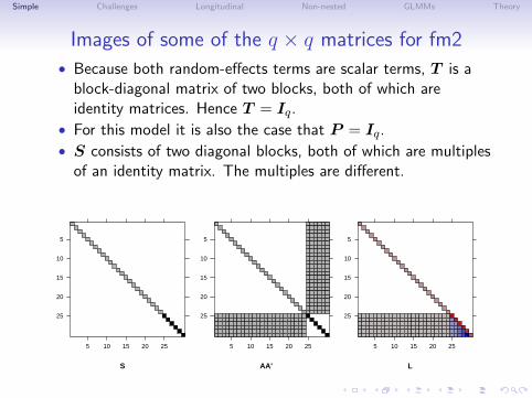
Images of some of the q × q matrices for fm2
• Because both random-effects terms are scalar terms, T is ablock-diagonal matrix of two blocks, both of which areidentity matrices. Hence T = Iq.
• For this model it is also the case that P = Iq.
• S consists of two diagonal blocks, both of which are multiplesof an identity matrix. The multiples are different.
S
5
10
15
20
25
5 10 15 20 25
AA'
5
10
15
20
25
5 10 15 20 25
L
5
10
15
20
25
5 10 15 20 25

Simple Challenges Longitudinal Non-nested GLMMs Theory
Recap of the Penicillin model
• The model formula isdiameter ~ 1 + (1 | plate) + (1 | sample)
• There are two random-effects terms, (1|plate) and(1|sample). Both are simple, scalar (q1 = q2 = 1) randomeffects terms, with n1 = 24 and n2 = 6 levels, respectively.Thus q = q1n1 + q2n2 = 30.
• The model matrix Z is the 144× 30 matrix created from twosets of indicator columns.
• The relative variance-covariance matrix, Σ, is block diagonalin two blocks that are nonnegative multiples of identitymatrices. The matrices AA′ and L show the crossing of thefactors. L has some fill-in relative to AA′.
• The fixed-effects parameter vector, β, is of length p = 1. Allthe elements of the 144× 1 model matrix X are unity.
Simple Challenges Longitudinal Non-nested GLMMs Theory
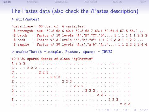
The Pastes data (also check the ?Pastes description)
> str(Pastes)
’data.frame’: 60 obs. of 4 variables:
$ strength: num 62.8 62.6 60.1 62.3 62.7 63.1 60 61.4 57.5 56.9 ...
$ batch : Factor w/ 10 levels "A","B","C","D",..: 1 1 1 1 1 1 2 2 2 2 ...
$ cask : Factor w/ 3 levels "a","b","c": 1 1 2 2 3 3 1 1 2 2 ...
$ sample : Factor w/ 30 levels "A:a","A:b","A:c",..: 1 1 2 2 3 3 4 4 5 5 ...
> xtabs(~batch + sample, Pastes, sparse = TRUE)
10 x 30 sparse Matrix of class "dgCMatrix"
A 2 2 2 . . . . . . . . . . . . . . . . . . . . . . . . . . .
B . . . 2 2 2 . . . . . . . . . . . . . . . . . . . . . . . .
C . . . . . . 2 2 2 . . . . . . . . . . . . . . . . . . . . .
D . . . . . . . . . 2 2 2 . . . . . . . . . . . . . . . . . .
E . . . . . . . . . . . . 2 2 2 . . . . . . . . . . . . . . .
F . . . . . . . . . . . . . . . 2 2 2 . . . . . . . . . . . .
G . . . . . . . . . . . . . . . . . . 2 2 2 . . . . . . . . .
H . . . . . . . . . . . . . . . . . . . . . 2 2 2 . . . . . .
I . . . . . . . . . . . . . . . . . . . . . . . . 2 2 2 . . .
J . . . . . . . . . . . . . . . . . . . . . . . . . . . 2 2 2
Simple Challenges Longitudinal Non-nested GLMMs Theory
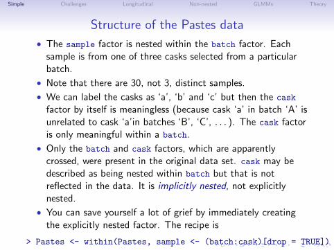
Structure of the Pastes data
• The sample factor is nested within the batch factor. Eachsample is from one of three casks selected from a particularbatch.
• Note that there are 30, not 3, distinct samples.
• We can label the casks as ‘a’, ‘b’ and ‘c’ but then the cask
factor by itself is meaningless (because cask ‘a’ in batch ‘A’ isunrelated to cask ‘a’in batches ‘B’, ‘C’, . . . ). The cask factoris only meaningful within a batch.
• Only the batch and cask factors, which are apparentlycrossed, were present in the original data set. cask may bedescribed as being nested within batch but that is notreflected in the data. It is implicitly nested, not explicitlynested.
• You can save yourself a lot of grief by immediately creatingthe explicitly nested factor. The recipe is
> Pastes <- within(Pastes, sample <- (batch:cask)[drop = TRUE])
Simple Challenges Longitudinal Non-nested GLMMs Theory
Avoid implicitly nested representations
• The lme4 package allows for very general model specifications.It does not require that factors associated with random effectsbe hierarchical or “multilevel” factors in the design.
• The same model specification can be used for data withnested or crossed or partially crossed factors. Nesting orcrossing is determined from the structure of the factors in thedata, not the model specification.
• You can avoid confusion about nested and crossed factors byfollowing one simple rule: ensure that different levels of afactor in the experiment correspond to different labels of thefactor in the data.
• Samples were drawn from 30, not 3, distinct casks in thisexperiment. We should specify models using the sample factorwith 30 levels, not the cask factor with 3 levels.
Simple Challenges Longitudinal Non-nested GLMMs Theory
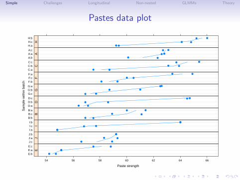
Pastes data plot
Paste strength
Sam
ple
with
in b
atch
E:bE:aE:c
54 56 58 60 62 64 66
●●
●●
●●
E
J:cJ:aJ:b
● ●
●●
●●
J
I:aI:cI:b
●●
●●
●●I
B:bB:cB:a ● ●
●●
●●B
D:aD:bD:c
●●
● ●
●●
D
G:cG:bG:a ●●
●●
● ●
G
F:bF:cF:a ● ●
●●
●●F
C:aC:bC:c
●●
●●
●●
C
A:bA:aA:c
●●
● ●
● ●
A
H:aH:cH:b
● ●
● ●
●●H
Simple Challenges Longitudinal Non-nested GLMMs Theory
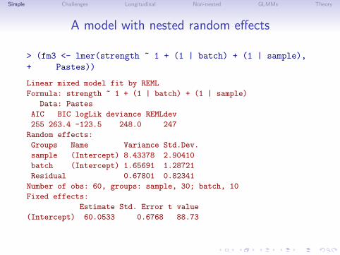
A model with nested random effects
> (fm3 <- lmer(strength ~ 1 + (1 | batch) + (1 | sample),+ Pastes))
Linear mixed model fit by REML
Formula: strength ~ 1 + (1 | batch) + (1 | sample)
Data: Pastes
AIC BIC logLik deviance REMLdev
255 263.4 -123.5 248.0 247
Random effects:
Groups Name Variance Std.Dev.
sample (Intercept) 8.43378 2.90410
batch (Intercept) 1.65691 1.28721
Residual 0.67801 0.82341
Number of obs: 60, groups: sample, 30; batch, 10
Fixed effects:
Estimate Std. Error t value
(Intercept) 60.0533 0.6768 88.73
Simple Challenges Longitudinal Non-nested GLMMs Theory
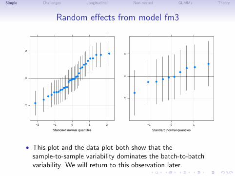
Random effects from model fm3
Standard normal quantiles
−5
05
−2 −1 0 1 2
●
●
●●
● ● ●● ●
●●●
●●●●●
●●
●
●●
●●
●
● ●
● ●●
Standard normal quantiles
−2
02
−1 0 1
●
● ●
●● ●
●
● ●
●
• This plot and the data plot both show that thesample-to-sample variability dominates the batch-to-batchvariability. We will return to this observation later.
Simple Challenges Longitudinal Non-nested GLMMs Theory
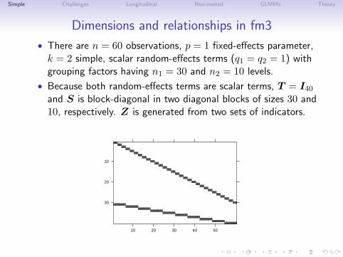
Dimensions and relationships in fm3
• There are n = 60 observations, p = 1 fixed-effects parameter,k = 2 simple, scalar random-effects terms (q1 = q2 = 1) withgrouping factors having n1 = 30 and n2 = 10 levels.
• Because both random-effects terms are scalar terms, T = I40
and S is block-diagonal in two diagonal blocks of sizes 30 and10, respectively. Z is generated from two sets of indicators.
10
20
30
10 20 30 40 50
Simple Challenges Longitudinal Non-nested GLMMs Theory
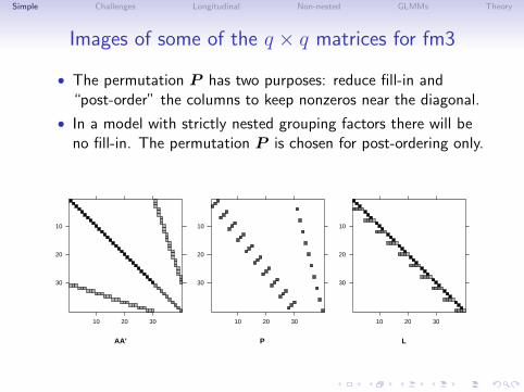
Images of some of the q × q matrices for fm3
• The permutation P has two purposes: reduce fill-in and“post-order” the columns to keep nonzeros near the diagonal.
• In a model with strictly nested grouping factors there will beno fill-in. The permutation P is chosen for post-ordering only.
AA'
10
20
30
10 20 30
P
10
20
30
10 20 30
L
10
20
30
10 20 30
Simple Challenges Longitudinal Non-nested GLMMs Theory
Eliminate the random-effects term for batch?
• We have seen that there is little batch-to-batch variabilitybeyond that induced by the variability of samples withinbatches.
• We can fit a reduced model without that term and compare itto the original model.
• Somewhat confusingly, model comparisons from likelihoodratio tests are obtained by calling the anova function on thetwo models. (Put the simpler model first in the call to anova.)
• Sometimes likelihood ratio tests can be evaluated using theREML criterion and sometimes they can’t. Instead of learningthe rules of when you can and when you can’t, it is easiestalways to refit the models with REML = FALSE beforecomparing.
Simple Challenges Longitudinal Non-nested GLMMs Theory
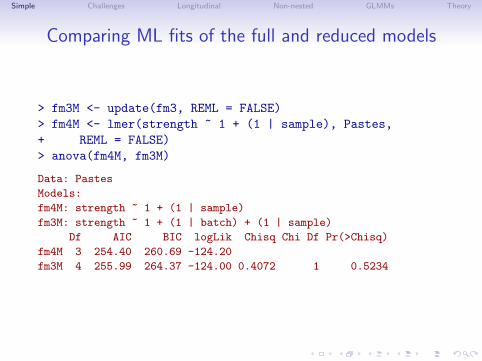
Comparing ML fits of the full and reduced models
> fm3M <- update(fm3, REML = FALSE)> fm4M <- lmer(strength ~ 1 + (1 | sample), Pastes,+ REML = FALSE)> anova(fm4M, fm3M)
Data: Pastes
Models:
fm4M: strength ~ 1 + (1 | sample)
fm3M: strength ~ 1 + (1 | batch) + (1 | sample)
Df AIC BIC logLik Chisq Chi Df Pr(>Chisq)
fm4M 3 254.40 260.69 -124.20
fm3M 4 255.99 264.37 -124.00 0.4072 1 0.5234
Simple Challenges Longitudinal Non-nested GLMMs Theory
p-values of LR tests on variance components
• The likelihood ratio is a reasonable criterion for comparingthese two models. However, the theory behind using a χ2
distribution with 1 degree of freedom as a referencedistribution for this test statistic does not apply in this case.The null hypothesis is on the boundary of the alternativehypothesis.
• Even at the best of times, the p-values for such tests are onlyapproximate because they are based on the asymptoticbehavior of the test statistic. To carry the argument further,all results in statistics are based on models and, as GeorgeBox famously said, “All models are wrong; some models areuseful.”
Simple Challenges Longitudinal Non-nested GLMMs Theory
LR tests on variance components (cont’d)
• In this case the problem with the boundary condition resultsin a p-value that is larger than it would be if, say, youcompared this likelihood ratio to values obtained for datasimulated from the null hypothesis model. We say theseresults are “conservative”.
• As a rule of thumb, the p-value for a simple, scalar term isroughly twice as large as it should be.
• In this case, dividing the p-value in half would not affect ourconclusion.
Simple Challenges Longitudinal Non-nested GLMMs Theory
Updated model, REML estimates
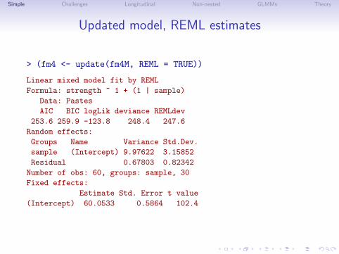
> (fm4 <- update(fm4M, REML = TRUE))
Linear mixed model fit by REML
Formula: strength ~ 1 + (1 | sample)
Data: Pastes
AIC BIC logLik deviance REMLdev
253.6 259.9 -123.8 248.4 247.6
Random effects:
Groups Name Variance Std.Dev.
sample (Intercept) 9.97622 3.15852
Residual 0.67803 0.82342
Number of obs: 60, groups: sample, 30
Fixed effects:
Estimate Std. Error t value
(Intercept) 60.0533 0.5864 102.4
Simple Challenges Longitudinal Non-nested GLMMs Theory
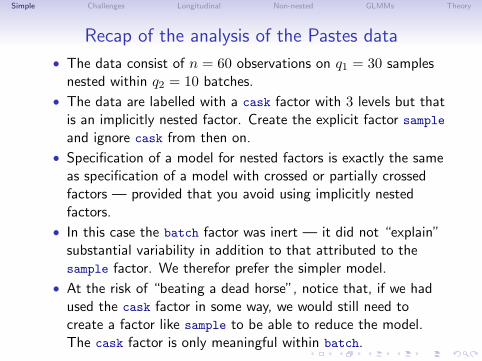
Recap of the analysis of the Pastes data
• The data consist of n = 60 observations on q1 = 30 samplesnested within q2 = 10 batches.
• The data are labelled with a cask factor with 3 levels but thatis an implicitly nested factor. Create the explicit factor sampleand ignore cask from then on.
• Specification of a model for nested factors is exactly the sameas specification of a model with crossed or partially crossedfactors — provided that you avoid using implicitly nestedfactors.
• In this case the batch factor was inert — it did not “explain”substantial variability in addition to that attributed to thesample factor. We therefor prefer the simpler model.
• At the risk of “beating a dead horse”, notice that, if we hadused the cask factor in some way, we would still need tocreate a factor like sample to be able to reduce the model.The cask factor is only meaningful within batch.
Simple Challenges Longitudinal Non-nested GLMMs Theory
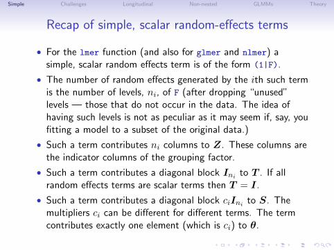
Recap of simple, scalar random-effects terms
• For the lmer function (and also for glmer and nlmer) asimple, scalar random effects term is of the form (1|F).
• The number of random effects generated by the ith such termis the number of levels, ni, of F (after dropping “unused”levels — those that do not occur in the data. The idea ofhaving such levels is not as peculiar as it may seem if, say, youfitting a model to a subset of the original data.)
• Such a term contributes ni columns to Z. These columns arethe indicator columns of the grouping factor.
• Such a term contributes a diagonal block Ini to T . If allrandom effects terms are scalar terms then T = I.
• Such a term contributes a diagonal block ciIni to S. Themultipliers ci can be different for different terms. The termcontributes exactly one element (which is ci) to θ.

Simple Challenges Longitudinal Non-nested GLMMs Theory
This is all very nice, but . . .• These methods are interesting but the results are not really
new. Similar results are quoted in Statistical Methods inResearch and Production, which is a very old book.
• The approach described in that book is actually quitesophisticated, especially when you consider that the methodsdescribed there, based on observed and expected meansquares, are for hand calculation (in pre-calculator days)!
• Why go to all the trouble of working with sparse matrices andall that if you could get the same results with paper andpencil? The one-word answer is balance.
• Those methods depend on the data being balanced. Thedesign must be completely balanced and the resulting datamust also be completely balanced.
• Balance is fragile. Even if the design is balanced, a singlemissing or questionable observation destroys the balance.Observational studies (as opposed to, say, laboratoryexperiments) cannot be expected to yield balanced data sets.
• Also, the models involve only simple, scalar random effectsand do not incorporate covariates.
Simple Challenges Longitudinal Non-nested GLMMs Theory
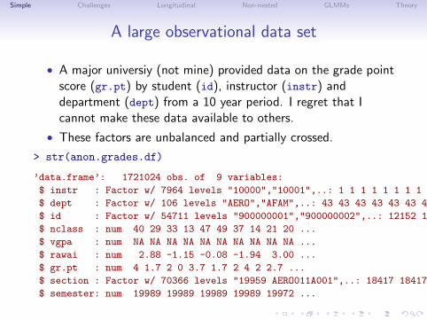
A large observational data set
• A major universiy (not mine) provided data on the grade pointscore (gr.pt) by student (id), instructor (instr) anddepartment (dept) from a 10 year period. I regret that Icannot make these data available to others.
• These factors are unbalanced and partially crossed.
> str(anon.grades.df)
’data.frame’: 1721024 obs. of 9 variables:
$ instr : Factor w/ 7964 levels "10000","10001",..: 1 1 1 1 1 1 1 1 1 1 ...
$ dept : Factor w/ 106 levels "AERO","AFAM",..: 43 43 43 43 43 43 43 43 43 43 ...
$ id : Factor w/ 54711 levels "900000001","900000002",..: 12152 1405 23882 18875 18294 20922 4150 13540 5499 6425 ...
$ nclass : num 40 29 33 13 47 49 37 14 21 20 ...
$ vgpa : num NA NA NA NA NA NA NA NA NA NA ...
$ rawai : num 2.88 -1.15 -0.08 -1.94 3.00 ...
$ gr.pt : num 4 1.7 2 0 3.7 1.7 2 4 2 2.7 ...
$ section : Factor w/ 70366 levels "19959 AERO011A001",..: 18417 18417 18417 18417 9428 18417 18417 9428 9428 9428 ...
$ semester: num 19989 19989 19989 19989 19972 ...
Simple Challenges Longitudinal Non-nested GLMMs Theory
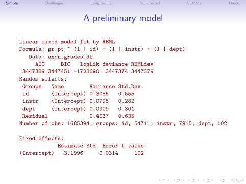
A preliminary model
Linear mixed model fit by REML
Formula: gr.pt ~ (1 | id) + (1 | instr) + (1 | dept)
Data: anon.grades.df
AIC BIC logLik deviance REMLdev
3447389 3447451 -1723690 3447374 3447379
Random effects:
Groups Name Variance Std.Dev.
id (Intercept) 0.3085 0.555
instr (Intercept) 0.0795 0.282
dept (Intercept) 0.0909 0.301
Residual 0.4037 0.635
Number of obs: 1685394, groups: id, 54711; instr, 7915; dept, 102
Fixed effects:
Estimate Std. Error t value
(Intercept) 3.1996 0.0314 102
Simple Challenges Longitudinal Non-nested GLMMs Theory
Comments on the model fit
• n = 1685394, p = 1, k = 3, n1 = 54711, n2 = 7915,n3 = 102, q1 = q2 = q3 = 1, q = 62728
• This model is sometimes called the “unconditional” model inthat it does not incorporate covariates beyond the groupingfactors.
• It takes less than an hour to fit an ”unconditional” modelwith random effects for student (id), instructor (inst) anddepartment (dept) to these data.
• Naturally, this is just the first step. We want to look atpossible time trends and the possible influences of thecovariates.
Simple Challenges Longitudinal Non-nested GLMMs Theory
Challenges in fitting mixed models
• Like all statistical models, linear mixed models are being fit tolarger and larger data sets - microarray data, massivelongitudinal studies, genetic studies with pedigrees, etc.
• The structure of the models being fit is also getting morecomplex. Observational longitudinal studies with multiplelevels of grouping (e.g. test scores by student, teacher, school,district, . . . ) may have non-nested groupings (a particularstudent is exposed to more than one teacher/schoolcombination). Or we could be modeling data classified byfully crossed factors such as subject and item.
• We wish to allow for generalizations such as generalized linearmixed models (GLMMs) or nonlinear mixed models (NLMMs)or even generalized nonlinear mixed models (GNMMs).
Simple Challenges Longitudinal Non-nested GLMMs Theory
Looking at the “big picture”
• Most descriptions of mixed-effects models concentrate on thedetails, sometimes degenerating into subscript fests. As inmany complex systems, it is valuable before considering thedetails to step back and look at the big picture.
• We consider mixed models for an n-dimensional response ymodeled as a random variable Y . The random effects, B, areanother vector-valued random variable in the model.
• The model specifies the conditional distribution, Y |B, and themarginal distribution, B, as depending on parameters.
• The marginal distribution, B, has the form
B ∼ N(0, σ2Σ(θ)
)where θ is the variance-component parameter vector. Not allmodels incorporate a common scale parameter, σ. When it isused, it also occurs in the formulation of the conditionaldistribution, Y |B.
Simple Challenges Longitudinal Non-nested GLMMs Theory
The conditional distribution, Y |B• The conditional mean,
µY|B(b) = E[Y |B = b] = g−1(η),
depends on the unbounded predictor, η, through the inverselink, g−1. For LMMs and GLMMs, η is a linear predictor,
η = Xβ + Zb.
• The conditional distribution, (Y |B = b), is completelydetermined by the conditional mean, µY|B, and, perhaps, thecommon scale parameter, σ.
• Components of Y are conditionally independent, given B.Thus, the conditional distribution, (Y |B = b), is determinedby the (scalar) distribution of each component. Furthermore,the inverse link, g−1, is determined by a scalar function g−1
applied componentwise.
Simple Challenges Longitudinal Non-nested GLMMs Theory
The unscaled conditional density of (B|Y = y)
• We observe y. To make inferences about B we want theconditional distribution (B|Y = y), not (Y |B = b).
• Although the response random variable, Y , may be discrete orcontinuous, the random effects, B, are always a continuousvector-valued random variable.
• Given values of θ, β and, if used, σ we can evaluate thedensity of (B|Y = y) for any value of b, but only up to ascale factor.
• The inverse of the scale factor,∫Rq
[(Y |B = b)(y)][B(b)] db,
is exactly the likelihood, L(θ,β, σ2|y), of the parametersgiven the data.
Simple Challenges Longitudinal Non-nested GLMMs Theory
The conditional mode of B• To evaluate the likelihood, L(θ,β, σ2|y), at a particular set of
parameter values, we first evaluate the conditional mode ofthe random effects,
b(θ,β) = arg maxb
[(Y |B = b)(y)][(B)(b)]
(σ does not affect the conditional mode.)
• This optimization problem is easy (well, relatively easy)because it can be expressed as a penalized least squares (PLS)problem. Even better, the PLS problem expressed in terms oforthogonal random effects, U ∼ N (0, σ2Iq), whereB = T (θ)S(θ)U , has a simple form
u(θ,β) = arg minu
∥∥∥∥[W 1/2
(y − µY|U (u)
)u
]∥∥∥∥2
where the diagonal matrix of weights, W , depends only onµY|U (and, hence, only on η).
Simple Challenges Longitudinal Non-nested GLMMs Theory
Penalized (whatever) least squares methods• The reason that the PLS problem for determining the
conditional modes is relatively easy is because the standardleast squares-based methods for fixed-effects models are easilyadapted.
• For linear mixed-models the PLS problem is solved directly. Infact, for LMMs it is possible to determine the conditionalmodes of the random effects and the conditional estimates ofthe fixed effects simultaneously.
• Parameter estimates for generalized linear models (GLMs) are(very efficiently) determined by iteratively re-weighted leastsquares (IRLS) so the conditional modes in a GLMM aredetermined by penalized iteratively re-weighted least squares(PIRLS).
• Nonlinear least squares, used for fixed-effects nonlinearregression, is adapted as penalized nonlinear least squares(PNLS) or penalized iteratively reweighted nonlinear leastsquares (PIRNLS) for generalized nonlinear mixed models.
Simple Challenges Longitudinal Non-nested GLMMs Theory
Simple longitudinal data
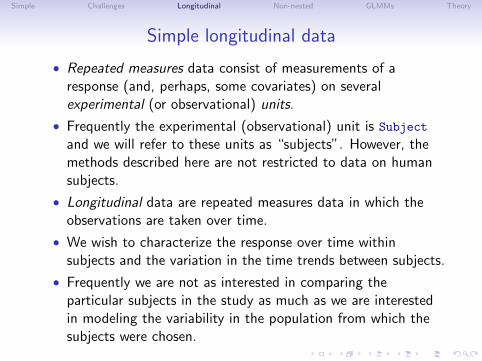
• Repeated measures data consist of measurements of aresponse (and, perhaps, some covariates) on severalexperimental (or observational) units.
• Frequently the experimental (observational) unit is Subject
and we will refer to these units as “subjects”. However, themethods described here are not restricted to data on humansubjects.
• Longitudinal data are repeated measures data in which theobservations are taken over time.
• We wish to characterize the response over time withinsubjects and the variation in the time trends between subjects.
• Frequently we are not as interested in comparing theparticular subjects in the study as much as we are interestedin modeling the variability in the population from which thesubjects were chosen.
Simple Challenges Longitudinal Non-nested GLMMs Theory
Sleep deprivation data
• This laboratory experiment measured the effect of sleepdeprivation on cognitive performance.
• There were 18 subjects, chosen from the population ofinterest (long-distance truck drivers), in the 10 day trial.These subjects were restricted to 3 hours sleep per nightduring the trial.
• On each day of the trial each subject’s reaction time wasmeasured. The reaction time shown here is the average ofseveral measurements.
• These data are balanced in that each subject is measured thesame number of times and on the same occasions.
Simple Challenges Longitudinal Non-nested GLMMs Theory
Reaction time versus days by subject
Days of sleep deprivation
Ave
rage
rea
ctio
n tim
e (m
s)
200
250
300
350
400
450
0 2 4 6 8
● ●
● ● ●●
●
● ●●
310
●● ● ● ●
● ● ● ●●
309
0 2 4 6 8
●● ● ●
●
●
●
●● ●
370
● ●●
● ●●
●
●
●●
349
0 2 4 6 8
●●
● ●●
●
●●
● ●
350
●●
●●
● ●
●
● ●
●
334
0 2 4 6 8
●●
●
●
●
●
●
●
●
●
308
● ● ● ● ● ●
●
●
●●
371
0 2 4 6 8
● ●●
●
● ●●
●●
●
369
●
●
●●
●
●●
●
●
●
351
0 2 4 6 8
●
●
●●
● ●●
● ● ●
335
●●
●
● ● ●
●
●●
●
332
0 2 4 6 8
● ●
●●
●
● ●●
● ●
372
● ●●
● ●
● ●●
●
●
333
0 2 4 6 8
●
●
●
● ● ● ● ●●
●
352
● ●●
● ●
● ●
●
●
●
331
0 2 4 6 8
●
●● ● ●
●●
●●
●
330
200
250
300
350
400
450
● ●
●
●
●
●●
●
● ●
337
Simple Challenges Longitudinal Non-nested GLMMs Theory
Comments on the sleep data plot
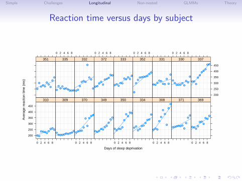
• The plot is a “trellis” or “lattice” plot where the data for eachsubject are presented in a separate panel. The axes areconsistent across panels so we may compare patterns acrosssubjects.
• A reference line fit by simple linear regression to the panel’sdata has been added to each panel.
• The aspect ratio of the panels has been adjusted so that atypical reference line lies about 45◦ on the page. We have thegreatest sensitivity in checking for differences in slopes whenthe lines are near ±45◦ on the page.
• The panels have been ordered not by subject number (whichis essentially a random order) but according to increasingintercept for the simple linear regression. If the slopes and theintercepts are highly correlated we should see a pattern acrossthe panels in the slopes.
Simple Challenges Longitudinal Non-nested GLMMs Theory
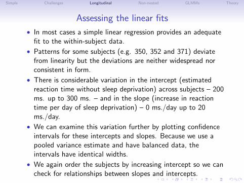
Assessing the linear fits
• In most cases a simple linear regression provides an adequatefit to the within-subject data.
• Patterns for some subjects (e.g. 350, 352 and 371) deviatefrom linearity but the deviations are neither widespread norconsistent in form.
• There is considerable variation in the intercept (estimatedreaction time without sleep deprivation) across subjects – 200ms. up to 300 ms. – and in the slope (increase in reactiontime per day of sleep deprivation) – 0 ms./day up to 20ms./day.
• We can examine this variation further by plotting confidenceintervals for these intercepts and slopes. Because we use apooled variance estimate and have balanced data, theintervals have identical widths.
• We again order the subjects by increasing intercept so we cancheck for relationships between slopes and intercepts.
Simple Challenges Longitudinal Non-nested GLMMs Theory
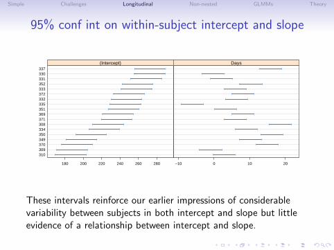
95% conf int on within-subject intercept and slope
310309370349350334308371369351335332372333352331330337
180 200 220 240 260 280
|
|
|
|
|
|
|
|
|
|
|
|
|
|
|
|
|
|
|
|
|
|
|
|
|
|
|
|
|
|
|
|
|
|
|
|
(Intercept)
−10 0 10 20
|
|
|
|
|
|
|
|
|
|
|
|
|
|
|
|
|
|
|
|
|
|
|
|
|
|
|
|
|
|
|
|
|
|
|
|
Days
These intervals reinforce our earlier impressions of considerablevariability between subjects in both intercept and slope but littleevidence of a relationship between intercept and slope.
Simple Challenges Longitudinal Non-nested GLMMs Theory
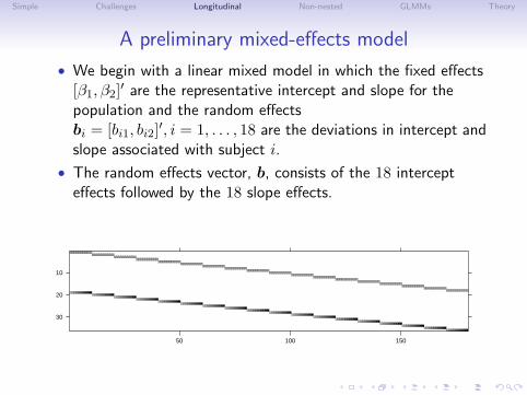
A preliminary mixed-effects model
• We begin with a linear mixed model in which the fixed effects[β1, β2]′ are the representative intercept and slope for thepopulation and the random effectsbi = [bi1, bi2]′, i = 1, . . . , 18 are the deviations in intercept andslope associated with subject i.
• The random effects vector, b, consists of the 18 intercepteffects followed by the 18 slope effects.
10
20
30
50 100 150
Simple Challenges Longitudinal Non-nested GLMMs Theory
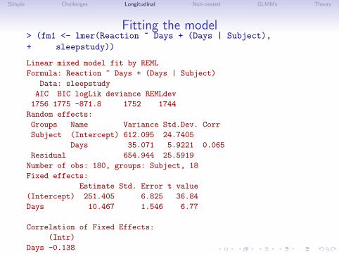
Fitting the model> (fm1 <- lmer(Reaction ~ Days + (Days | Subject),+ sleepstudy))
Linear mixed model fit by REML
Formula: Reaction ~ Days + (Days | Subject)
Data: sleepstudy
AIC BIC logLik deviance REMLdev
1756 1775 -871.8 1752 1744
Random effects:
Groups Name Variance Std.Dev. Corr
Subject (Intercept) 612.095 24.7405
Days 35.071 5.9221 0.065
Residual 654.944 25.5919
Number of obs: 180, groups: Subject, 18
Fixed effects:
Estimate Std. Error t value
(Intercept) 251.405 6.825 36.84
Days 10.467 1.546 6.77
Correlation of Fixed Effects:
(Intr)
Days -0.138
Simple Challenges Longitudinal Non-nested GLMMs Theory
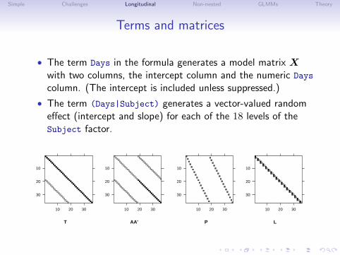
Terms and matrices
• The term Days in the formula generates a model matrix Xwith two columns, the intercept column and the numeric Days
column. (The intercept is included unless suppressed.)
• The term (Days|Subject) generates a vector-valued randomeffect (intercept and slope) for each of the 18 levels of theSubject factor.
T
10
20
30
10 20 30
AA'
10
20
30
10 20 30
P
10
20
30
10 20 30
L
10
20
30
10 20 30
Simple Challenges Longitudinal Non-nested GLMMs Theory
A model with uncorrelated random effects
• The data plots gave little indication of a systematicrelationship between a subject’s random effect for slope andhis/her random effect for the intercept. Also, the estimatedcorrelation is quite small.
• We should consider a model with uncorrelated random effects.To express this we use two random-effects terms with thesame grouping factor and different left-hand sides. In theformula for an lmer model, distinct random effects terms aremodeled as being independent. Thus we specify the modelwith two distinct random effects terms, each of which hasSubject as the grouping factor. The model matrix for oneterm is intercept only (1) and for the other term is the columnfor Days only, which can be written 0+Days. (The expressionDays generates a column for Days and an intercept. Tosuppress the intercept we add 0+ to the expression; -1 alsoworks.)
Simple Challenges Longitudinal Non-nested GLMMs Theory
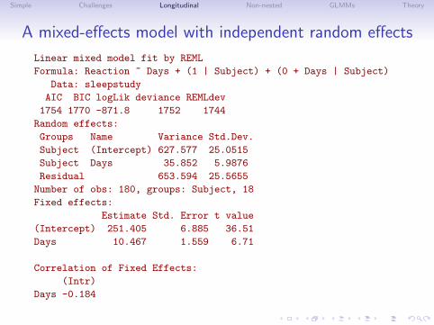
A mixed-effects model with independent random effects
Linear mixed model fit by REML
Formula: Reaction ~ Days + (1 | Subject) + (0 + Days | Subject)
Data: sleepstudy
AIC BIC logLik deviance REMLdev
1754 1770 -871.8 1752 1744
Random effects:
Groups Name Variance Std.Dev.
Subject (Intercept) 627.577 25.0515
Subject Days 35.852 5.9876
Residual 653.594 25.5655
Number of obs: 180, groups: Subject, 18
Fixed effects:
Estimate Std. Error t value
(Intercept) 251.405 6.885 36.51
Days 10.467 1.559 6.71
Correlation of Fixed Effects:
(Intr)
Days -0.184
Simple Challenges Longitudinal Non-nested GLMMs Theory
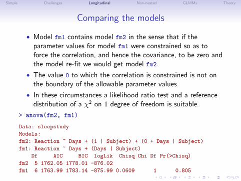
Comparing the models
• Model fm1 contains model fm2 in the sense that if theparameter values for model fm1 were constrained so as toforce the correlation, and hence the covariance, to be zero andthe model re-fit we would get model fm2.
• The value 0 to which the correlation is constrained is not onthe boundary of the allowable parameter values.
• In these circumstances a likelihood ratio test and a referencedistribution of a χ2 on 1 degree of freedom is suitable.
> anova(fm2, fm1)
Data: sleepstudy
Models:
fm2: Reaction ~ Days + (1 | Subject) + (0 + Days | Subject)
fm1: Reaction ~ Days + (Days | Subject)
Df AIC BIC logLik Chisq Chi Df Pr(>Chisq)
fm2 5 1762.05 1778.01 -876.02
fm1 6 1763.99 1783.14 -875.99 0.0609 1 0.805
Simple Challenges Longitudinal Non-nested GLMMs Theory
Conclusions from the likelihood ratio test
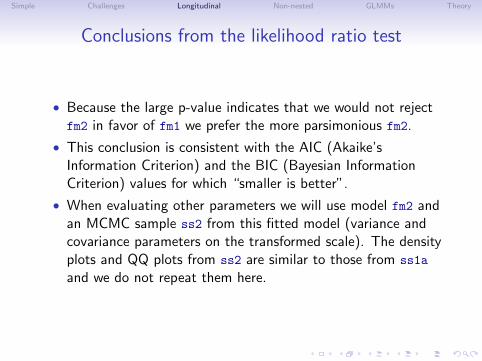
• Because the large p-value indicates that we would not rejectfm2 in favor of fm1 we prefer the more parsimonious fm2.
• This conclusion is consistent with the AIC (Akaike’sInformation Criterion) and the BIC (Bayesian InformationCriterion) values for which “smaller is better”.
• When evaluating other parameters we will use model fm2 andan MCMC sample ss2 from this fitted model (variance andcovariance parameters on the transformed scale). The densityplots and QQ plots from ss2 are similar to those from ss1a
and we do not repeat them here.
Simple Challenges Longitudinal Non-nested GLMMs Theory
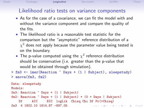
Likelihood ratio tests on variance components• As for the case of a covariance, we can fit the model with and
without the variance component and compare the quality ofthe fits.
• The likelihood ratio is a reasonable test statistic for thecomparison but the “asymptotic” reference distribution of aχ2 does not apply because the parameter value being tested ison the boundary.
• The p-value computed using the χ2 reference distributionshould be conservative (i.e. greater than the p-value thatwould be obtained through simulation).
> fm3 <- lmer(Reaction ~ Days + (1 | Subject), sleepstudy)> anova(fm3, fm2)
Data: sleepstudy
Models:
fm3: Reaction ~ Days + (1 | Subject)
fm2: Reaction ~ Days + (1 | Subject) + (0 + Days | Subject)
Df AIC BIC logLik Chisq Chi Df Pr(>Chisq)
fm3 4 1802.10 1814.87 -897.05
fm2 5 1762.05 1778.01 -876.02 42.053 1 8.885e-11
Simple Challenges Longitudinal Non-nested GLMMs Theory
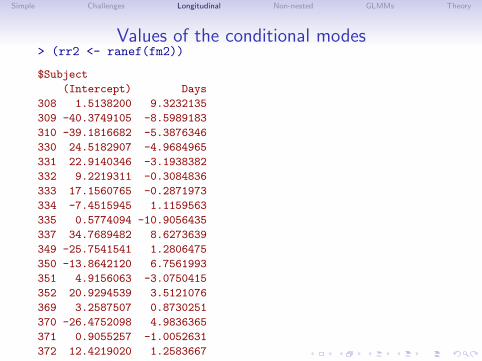
Values of the conditional modes> (rr2 <- ranef(fm2))
$Subject
(Intercept) Days
308 1.5138200 9.3232135
309 -40.3749105 -8.5989183
310 -39.1816682 -5.3876346
330 24.5182907 -4.9684965
331 22.9140346 -3.1938382
332 9.2219311 -0.3084836
333 17.1560765 -0.2871973
334 -7.4515945 1.1159563
335 0.5774094 -10.9056435
337 34.7689482 8.6273639
349 -25.7541541 1.2806475
350 -13.8642120 6.7561993
351 4.9156063 -3.0750415
352 20.9294539 3.5121076
369 3.2587507 0.8730251
370 -26.4752098 4.9836365
371 0.9055257 -1.0052631
372 12.4219020 1.2583667
Simple Challenges Longitudinal Non-nested GLMMs Theory
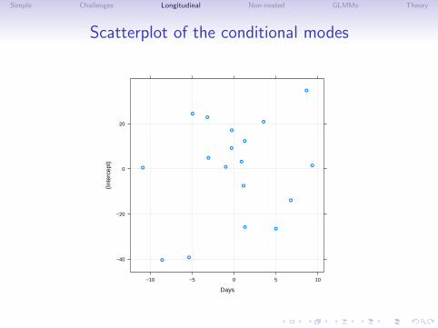
Scatterplot of the conditional modes
Days
(Int
erce
pt)
−40
−20
0
20
−10 −5 0 5 10
●
●●
●●
●
●
●
●
●
●
●
●
●
●
●
●
●
Simple Challenges Longitudinal Non-nested GLMMs Theory
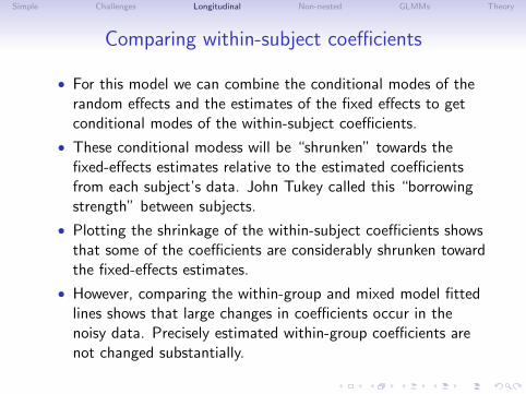
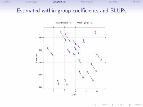
Comparing within-subject coefficients
• For this model we can combine the conditional modes of therandom effects and the estimates of the fixed effects to getconditional modes of the within-subject coefficients.
• These conditional modess will be “shrunken” towards thefixed-effects estimates relative to the estimated coefficientsfrom each subject’s data. John Tukey called this “borrowingstrength” between subjects.
• Plotting the shrinkage of the within-subject coefficients showsthat some of the coefficients are considerably shrunken towardthe fixed-effects estimates.
• However, comparing the within-group and mixed model fittedlines shows that large changes in coefficients occur in thenoisy data. Precisely estimated within-group coefficients arenot changed substantially.
Simple Challenges Longitudinal Non-nested GLMMs Theory
Estimated within-group coefficients and BLUPs
Days
(Int
erce
pt)
200
220
240
260
280
0 5 10 15 20
●
●●
●
●
●
●
●
●
●
●
●
●
●
●
●
●
●
●
●●
●●
●
●
●
●
●
●
●
●
●
●
●
●
●
Mixed model Within−group● ●
Simple Challenges Longitudinal Non-nested GLMMs Theory
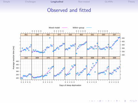
Observed and fitted
Days of sleep deprivation
Ave
rage
rea
ctio
n tim
e (m
s)
200
250
300
350
400
450
0 2 4 6 8
● ●
● ● ●●
●
● ●●
310
●● ● ● ●
● ● ● ●●
309
0 2 4 6 8
●● ● ●
●
●
●
●● ●
370
● ●●
● ●●
●
●
●●
349
0 2 4 6 8
●●
● ●●
●
●●
● ●
350
●●
●●
● ●
●
● ●
●
334
0 2 4 6 8
●●
●
●
●
●
●
●
●
●
308
● ● ● ● ● ●
●
●
●●
371
0 2 4 6 8
● ●●
●
● ●●
●●
●
369
●
●
●●
●
●●
●
●
●
351
0 2 4 6 8
●
●
●●
● ●●
● ● ●
335
●●
●
● ● ●
●
●●
●
332
0 2 4 6 8
● ●
●●
●
● ●●
● ●
372
● ●●
● ●
● ●●
●
●
333
0 2 4 6 8
●
●
●
● ● ● ● ●●
●
352
● ●●
● ●
● ●
●
●
●
331
0 2 4 6 8
●
●● ● ●
●●
●●
●
330
200
250
300
350
400
450
● ●
●
●
●
●●
●
● ●
337
Mixed model Within−group
Simple Challenges Longitudinal Non-nested GLMMs Theory
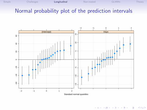
Prediction intervals on the random effects
• For the linear mixed model we can calculate both the meansand the variances of the random-effects conditional on theestimated values of the model parameters, which allows us tocalculate prediction intervals on the values of individualrandom effects.
• We plot the prediction intervals as a normal probabity plot sowe can see the overall shape of the distribution of the meansand which of the random effects are “significantly different”from zero.
• Note that failure of the conditional means of the randomeffects to look like a normal (Gaussian) distribution is notterribly alarming. It is the “prior” distribution of the randomeffects that is assumed to be normal. The conditional meansor BLUPs are strongly influenced by the data and may appearnon-normal.
Simple Challenges Longitudinal Non-nested GLMMs Theory
Normal probability plot of the prediction intervals
Standard normal quantiles
−60
−40
−20
020
4060
−2 −1 0 1 2
●●
● ●
●
●
● ●● ● ●
●●
●
●●
●
●
(Intercept)
−2 −1 0 1 2
−15
−10
−5
05
1015
●
●
●●
● ●
●● ●
● ● ● ●
●
●
●
●●
Days
Simple Challenges Longitudinal Non-nested GLMMs Theory
Conclusions from the example• Carefully plotting the data is enormously helpful in
formulating the model.• It is relatively easy to fit and evaluate models to data like
these, from a balanced designed experiment.• For a linear mixed model the estimates of the fixed effects
typically have a symmetric distribution close to a Gaussiandistribution.
• The distribution of the variance components or thecovariances are not symmetric, which is why we transformthese parameters to a symmetric scale.
• We use the MCMC sample to create confidence (actuallyHPD) intervals on the fixed-effects parameters. We could alsouse the parameter estimates and standard errors.
• The “estimates” (actually BLUPs) of the random effects canbe considered as penalized estimates of these parameters inthat they are shrunk towards the origin.
• Most of the prediction intervals for the random effects overlapzero.
Simple Challenges Longitudinal Non-nested GLMMs Theory
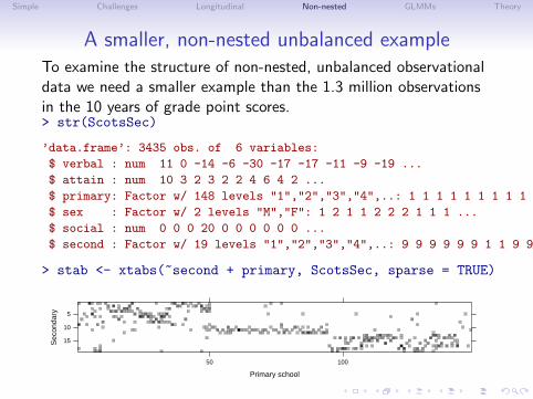
A smaller, non-nested unbalanced exampleTo examine the structure of non-nested, unbalanced observationaldata we need a smaller example than the 1.3 million observationsin the 10 years of grade point scores.> str(ScotsSec)
’data.frame’: 3435 obs. of 6 variables:
$ verbal : num 11 0 -14 -6 -30 -17 -17 -11 -9 -19 ...
$ attain : num 10 3 2 3 2 2 4 6 4 2 ...
$ primary: Factor w/ 148 levels "1","2","3","4",..: 1 1 1 1 1 1 1 1 1 1 ...
$ sex : Factor w/ 2 levels "M","F": 1 2 1 1 2 2 2 1 1 1 ...
$ social : num 0 0 0 20 0 0 0 0 0 0 ...
$ second : Factor w/ 19 levels "1","2","3","4",..: 9 9 9 9 9 9 1 1 9 9 ...
> stab <- xtabs(~second + primary, ScotsSec, sparse = TRUE)
Primary school
Sec
onda
ry 5
10
15
50 100
Simple Challenges Longitudinal Non-nested GLMMs Theory
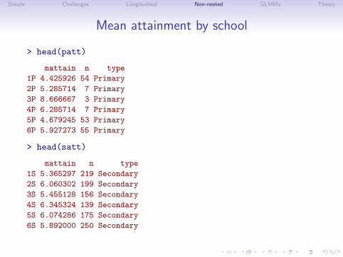
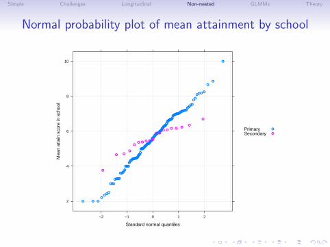
Mean attainment by school
> head(patt)
mattain n type
1P 4.425926 54 Primary
2P 5.285714 7 Primary
3P 8.666667 3 Primary
4P 6.285714 7 Primary
5P 4.679245 53 Primary
6P 5.927273 55 Primary
> head(satt)
mattain n type
1S 5.365297 219 Secondary
2S 6.060302 199 Secondary
3S 5.455128 156 Secondary
4S 6.345324 139 Secondary
5S 6.074286 175 Secondary
6S 5.892000 250 Secondary
Simple Challenges Longitudinal Non-nested GLMMs Theory
Normal probability plot of mean attainment by school
Standard normal quantiles
Mea
n at
tain
sco
re in
sch
ool
2
4
6
8
10
−2 −1 0 1 2
● ● ●
●●
●●
●●●
●●●●●
●●●●●●
●●●●●
●●●●●
●●●●●●●●●●●
●●●●●
●●●●●●●●●●●●●●●●●●●●
●●●●●●●●●
●●●●●
●●●●●●●●●●●●
●●●●●●●●●
●●●●●●
●●●●●●●●●●●
●●●●●●●●●
●●●●●●●●●●●
●●
●●● ●
●
●
●
●
● ●●
●● ● ● ● ●
● ●● ●
● ● ●●
●
PrimarySecondary
●
●
Simple Challenges Longitudinal Non-nested GLMMs Theory
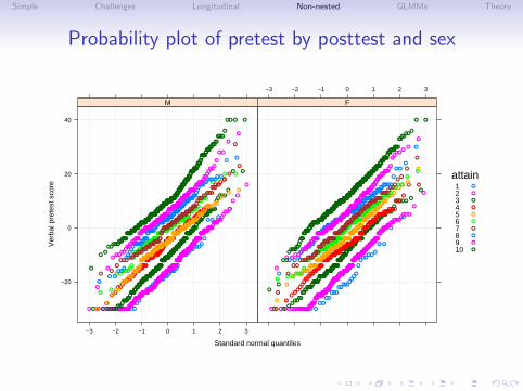
Probability plot of pretest by posttest and sex
Standard normal quantiles
Ver
bal p
rete
st s
core
−20
0
20
40
−3 −2 −1 0 1 2 3
● ● ● ●●●
●●
●●●
●●●●
●●●●
●●●●●●●●
●●●●●●
●●●
●●
●●●●●●
●●●●●
●
●
● ●●
●
● ● ●●●●●●●●●●●●●●●●●●●●●●●●●●●●●
●●●●●●●●●●●●●●●●●●●●●
●●●●●●●●●●●●●●●●●●●●●●●●●●●●●●●
●●●●●●●●●●●●●●●●●●●●●●●●●●●●●●●●●●
●●●●●●●●●●●●●●●●●●●●●●●●●●●●●●●●●
●●●●●●●●●●●●●●●●●●●●●●●●●●●●●●●●
●●●●●●●●●●●●●●●●●●●●●●●●●●●●●●●●●●●
●●●●●●●●●●●●●●●●●●●●●●
●●●●●●●●●●●●●●●●●●●●●●●●●●●●●●●●●●●●●
●●●●●●●●●●●●●●●●●●●●●●●●●●●●●●
●●●●●●●●●●●●●●●●●●●●●●●●●●●●●●●●●●●
●●●●●●●●●●●●●●●●●
●●●●●●●●●●●●●
●●●●●●●
●
●
●
●
● ● ●●●●●●●
●●●●●
●●●●●●●●●
●●●●●●●●●●●●
●●●●●●●●●●●●●
●●●●●●●●●●●●●●●●●●
●●●●●●●●●●●●●●●●●●●●
●●●●●●●●
●●●●●●●●●●●●●●●●●●●●●●●●●●
●●●●●●●●●●●●●●●●●
●●●●●●●●●●●●●●●●●●
●●●●●●●●●●●●●●●
●●●●●●●●
●●●●●●●●●●●●●●●●●
●●●●●●●●●●●●●●●●
●●●●●●●●
●●●●●●●
●●●●●
●
● ●
●
●
●●
●●●●●
●●●●●●
●●●●●●
●●●●●●●●●●●
●●●●●●●●●●●●●
●●●●●●●●●●●●●●●●
●●●●●●●●●●●●●●●●●●
●●●●●●●●●●●●●●
●●●●●●●●●●●●●
●●●●●●●●●●●●●●●●●●
●●●●●●●●●●●●●
●●●●●●●
●●●●●
●●
●●●
●●
●
●
●
●
●
●●
●●●●
●●●●
●●●●●
●●●●
●●●●●●●●●●
●●●●●●●●●●●●●●●●●●●
●●●●●●●●●●●●●●●●●●●●●
●●●●●●●●●●●●●●
●●●●●●●●●●●●●●●●●
●●●●●●●●●●●●●●●
●●●●●●●●●●●
●●●●●●
●●●●●●●●
●●
●●
●●
●●
● ●●●●
●●
●
●●●●●●
●●●●●●
●●●●●●●●●●●●●
●●●●●●●●●●●●●●●
●●●●●●●●●●●●
●●●●●●●●●●●●●
●●●●●●●●●
●●●●●●
●●●●●
●●
●● ●
● ●
●●
●
●●●●●●
●●●●●●●
●●●●●●●●
●●●●●●●●●●●●
●●
●●●●●●●●●●●
●●●●●●●●●●●
●●●●●●●●●
●●●●●●●●●
●●●●●●
●●●●●
●●●●
●●●
●
●
●
● ●
●●●
●●●●●●●●●●●●
●●●●●●●
●●●●●●●●●●
●●●●●●●●●●●●●●●●
●●●●●●●●●●●●●●●
●●●●●●●●●●●
●●●●●●●●
●●●●●●●●
●●●●●●●●
●●●●●●●
●●●●●●
●●
●●
●
●
●●●
●●●●●
●●●●●
●●●●
●●●●●●●●
●●●●●●●●●●●●●●●
●●●●●●●●●●●●●
●●●●●●●●●●●●●●●
●●●●●●●●●●●
●●●●●●●●●●●●●●
●●●●●●●●●
●●●●●●●●●●●●●●●●
●●●●●
●●●●●●●
●●●●
●
●
●●
●
●
●
●●
●●●●●●
●●●●●●●●
●●●●●●●●●●●●●●
●●●●●●●●●●●●●●
●●●●●●●●●●●●●●●●●●●●●●●●●
●●●●●●●●●●●●●●●●●●●●●●●●●
●●●●●●●●●●●●●●●●●●●●●●●
●●●●●●●●●●●●●●●●●●●●●●●●●●●
●●●●●●●●●●●●●●●●●●●●●●●●●●●●●●●●●●●●
●●●●●●●●●●●●●●●●●●●●●●●●●●●●●●●●●●●●●●●●●●●●●●●●●●●●●●
●●●●●●●●●●●●●●●●●
●●●●●●●●●●●●●●●●●●●●●●●●●●
●●●●●●
●●●●●●
●●
●●●●
●
●● ● ●
M
−3 −2 −1 0 1 2 3
● ● ● ●
●●
●●
●●●
●●●●●
●●●●
●
●●●
●●●
● ●
●
●
● ● ●●●●●●●●●●●●●●●●●●●●●●
●●●●●●●●●●●●●●●●●●●●●●●
●●●●●●●●●●●●●●●●●●●
●●●●●●●●●●●●●●●●●●●●●●●●●●●●●●●●
●●●●●●●●●●●●●●●●●●●●●●●●
●●●●●●●●●●●●●●●●●●●●●●●●●●
●●●●●●●●●●●●●
●●●●●●●●●●●●●●●●●●●●●●
●●●●●●●●●●●●●●●●●●●●●●●●
●●●●●●●●●●●●●●●●
●●●●●●●●●●●●●●●
●●●●●●●
●●●●●●●●●●
●●●●●●●●●●
●●●●●●●●
●●●●
●
●
● ●●
●●●
●●
●●●●
●●●●●●●●●●●●●●
●●●●●●●●●●●●
●●●●●●●●●●●●●●●
●●●●●●●●●●●●●●●●●●
●●●●●●●●●●●●●●●●●●●●●●●●
●●●●●●●●●●●●●●
●●●●●●●●●●●●●●●
●●●●●●●●●●●●●●●●●●●
●●●●●●●●●●●●
●●●●●●●●●●●●●
●●●●●●●●●●●●●
●●●●●●●●●●
●●
●●●●●●
●
●
●
●●
●●●●●●
●●●●●
●●●●●●●
●●●●
●●●●●●●●●●●●●●●
●●●●●●●●●●●●●●●●●●●
●●●●●●●●●●●●●●●●●
●●●●●●●●●●●●●●●●●●
●●●●●●●●●●●
●●●●●●●●●●●●●●●
●●●●●●●●●
●●●●●●●
●●●●●●●●●●
●●●●
●●
●
● ●
●
●
●●●●
●●●●●●●●●●●
●●●●●●●●●●
●●●●●●●●●●
●●●●●●●●●●●●●●●
●●●●●●●●●●●●
●●●●●●●●●●●●●●
●●●●●●●●●●●●●●
●●●●●●●●●●●
●●●●●●●
●●●●●●●●●●●●
●●●●●●
●●●●●●●●
●●●●
●
●●●
●
●
●● ●
●●●
●
●●●●●●
●●●●●●●
●●●●●●●●●●●
●●●●●●●●●●●●●●
●●●●●●●●
●●●●●●●●●●●
●●●●●●●●●●●●●●●●●●●
●●●●●●●●●●●●●●●●●
●●●●●●●●●
●●●●●●●●●
●●●●●
●●●●●●
●●●●
●
●
●
●
●●
●●●●●●●●
●●●●●
●●●●●●●
●●●●●●●●●●●●●●●●
●●●●●●●●●●●●●●
●●●●●●●●●●●●●●●●●
●●●●●●●●●●
●●●●●●●●●●
●●●●●●●●●●●
●●●●●●●●●
●●●●●
●●●●●●●●
●
●●
●
●
●
● ●●
●●●
●●●●
●●●●
●●●●●●
●●●●●●●●●●●
●●●●●●●●●●●●●
●●●●●●●●●●●●●
●●●●●●●●●●●●●●●●●
●●●●●●●●●●●
●●●●●●●●●●
●●●●●●
●●●●●●●
●
●●
●
●
●
● ●●●
●●●
●●●●
●●●●●●
●●●●●●●●●●●●●●
●●●●●●●●●●●●●●
●●●●●●●●●●●●●●●
●●●●●●●●●●●●
●●●●●●●●●●●●●●●●●●●
●●●●●●●●●●
●●●●●●●●
●●●●●●●●●●●●
●●●●●●●●●●●●●
●●●●●●
●●
●●
●●●
●
●
●
●
●●
●●●●●
●●●●●●●
●●●●●●●●●
●●●●●●●●
●●●●●●●●●●●●●●●●●●●●●●●●●●●
●●●●●●●●●●●●●●●●●●
●●●●●●●●●●●●●●●●●●●●●●●●●●●●●
●●●●●●●●●●●●●●●●●●●●●●●●●●●●●
●●●●●●●●●●●●●●●●●●●●●●●●●●●●●●●●●●●●●●●●
●●●●●●●●●●●●●●●●●●●●●●●●●●●●●●
●●●●●●●●●●●●●●●●●●●●●●●
●●●●●●●●●●●●●●●●●●●●●●●●●●●●
●●●●●●●●●●●●●●●●●●●●●●●●●●●●●●●●●●●
●●●●●●●●●●●●●●●●
●●●●●●●●●●●●●●●●●●●●●●●●●
●●●●●
●●●●●●●●●
●●●●
●●●
● ●
F
attain12345678910
●
●
●
●
●
●
●
●
●
●
Simple Challenges Longitudinal Non-nested GLMMs Theory
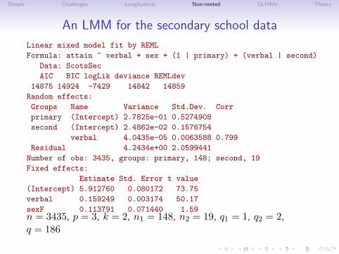
An LMM for the secondary school data
Linear mixed model fit by REML
Formula: attain ~ verbal + sex + (1 | primary) + (verbal | second)
Data: ScotsSec
AIC BIC logLik deviance REMLdev
14875 14924 -7429 14842 14859
Random effects:
Groups Name Variance Std.Dev. Corr
primary (Intercept) 2.7825e-01 0.5274908
second (Intercept) 2.4862e-02 0.1576754
verbal 4.0435e-05 0.0063588 0.799
Residual 4.2434e+00 2.0599441
Number of obs: 3435, groups: primary, 148; second, 19
Fixed effects:
Estimate Std. Error t value
(Intercept) 5.912760 0.080172 73.75
verbal 0.159249 0.003174 50.17
sexF 0.113791 0.071440 1.59n = 3435, p = 3, k = 2, n1 = 148, n2 = 19, q1 = 1, q2 = 2,q = 186
Simple Challenges Longitudinal Non-nested GLMMs Theory
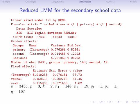
Reduced LMM for the secondary school data
Linear mixed model fit by REML
Formula: attain ~ verbal + sex + (1 | primary) + (1 | second)
Data: ScotsSec
AIC BIC logLik deviance REMLdev
14872 14909 -7430 14843 14860
Random effects:
Groups Name Variance Std.Dev.
primary (Intercept) 0.276261 0.52561
second (Intercept) 0.014455 0.12023
Residual 4.251960 2.06203
Number of obs: 3435, groups: primary, 148; second, 19
Fixed effects:
Estimate Std. Error t value
(Intercept) 5.919273 0.076151 77.73
verbal 0.159593 0.002778 57.46
sexF 0.115966 0.071463 1.62n = 3435, p = 3, k = 2, n1 = 148, n2 = 19, q1 = 1, q2 = 1,q = 167
Simple Challenges Longitudinal Non-nested GLMMs Theory
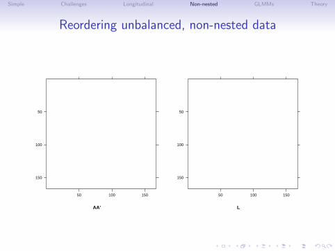
Reordering unbalanced, non-nested data
AA'
50
100
150
50 100 150
L
50
100
150
50 100 150
Simple Challenges Longitudinal Non-nested GLMMs Theory
Generalized linear mixed models• A generalized linear mixed model (GLMM) is used to model
repeated measures data with a non-normal distribution of theresponse conditional on the value of the linear predictor.
• Typically the data are binary (0/1) or binomial (k successesout of t trials) or a Poisson count.
• The formulation of the linear predictor is the same as in thelinear mixed model. However, the linear predictor is mappedto the conditional mean via a non-trivial “inverse link”function.
• The log-likelihood or, equivalently, the deviance of a GLMMdoes not have an explicit form in this case. As shown later,the marginal likelihood is expressed as an integral that doesnot have a closed-form solution.
• We use the Laplace approximation that involves determiningthe conditional modes of the random effects via PIRLS. Amore accurate alternative, adaptive Gauss-Hermite quadrature(AGQ) is being implemented as a Google Summer of Codeproject. However, AGQ is not universally applicable.

Simple Challenges Longitudinal Non-nested GLMMs Theory
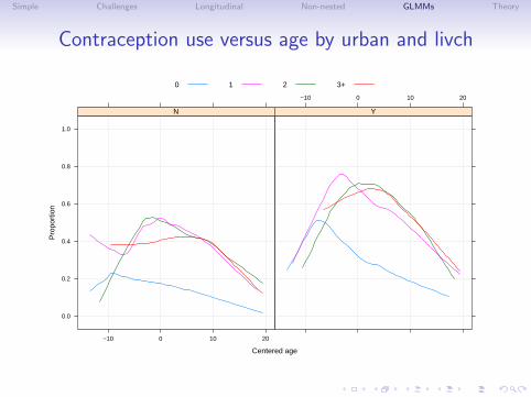
Contraception data
• One of the data sets in the "mlmRev" package, derived fromdata files available on the multilevel modelling web site, isfrom a fertility survey of women in Bangladesh.
• One of the responses is whether or not the woman currentlyuses artificial contraception (i.e. a binary response)
• Covariates included the woman’s age (on a centered scale),the number of live children she had, whether she lived in anurban or rural setting, and the district in which she lived.
• Instead of plotting such data as points, we use the 0/1response to generate scatterplot smoother curves versus agefor the different groups.
Simple Challenges Longitudinal Non-nested GLMMs Theory
Contraception use versus age by urban and livch
Centered age
Pro
port
ion
0.0
0.2
0.4
0.6
0.8
1.0
−10 0 10 20
N
−10 0 10 20
Y
0 1 2 3+
Simple Challenges Longitudinal Non-nested GLMMs Theory
Comments on the data plot
• These observational data are unbalanced (some districts haveonly 2 observations, some have nearly 120). They are notlongitudinal (no “time” variable).
• Binary responses have low per-observation informationcontent (exactly one bit per observation). Districts with fewobservations will not contribute strongly to estimates ofrandom effects.
• Within-district plots will be too imprecise so we only examinethe global effects in plots.
• The comparisons on the multilevel modelling site are for fits ofa model that is linear in age, which is clearly inappropriate.
• The form of the curves suggests at least a quadratic in age.
• The urban versus rural differences may be additive.
• It appears that the livch factor could be dichotomized into“0” versus “1 or more”.
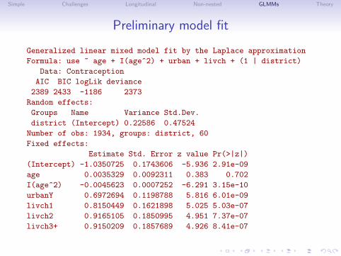
Simple Challenges Longitudinal Non-nested GLMMs Theory
Preliminary model fit
Generalized linear mixed model fit by the Laplace approximation
Formula: use ~ age + I(age^2) + urban + livch + (1 | district)
Data: Contraception
AIC BIC logLik deviance
2389 2433 -1186 2373
Random effects:
Groups Name Variance Std.Dev.
district (Intercept) 0.22586 0.47524
Number of obs: 1934, groups: district, 60
Fixed effects:
Estimate Std. Error z value Pr(>|z|)
(Intercept) -1.0350725 0.1743606 -5.936 2.91e-09
age 0.0035329 0.0092311 0.383 0.702
I(age^2) -0.0045623 0.0007252 -6.291 3.15e-10
urbanY 0.6972694 0.1198788 5.816 6.01e-09
livch1 0.8150449 0.1621898 5.025 5.03e-07
livch2 0.9165105 0.1850995 4.951 7.37e-07
livch3+ 0.9150209 0.1857689 4.926 8.41e-07
Simple Challenges Longitudinal Non-nested GLMMs Theory
Comments on the model fit
• There is a highly significant quadratic term in age.
• The linear term in age is not significant but we retain itbecause the age scale has been centered at an arbitrary (andunknown) value.
• The urban factor is highly significant (as indicated by theplot).
• Levels of livch greater than 0 are significantly different from0 but may not be different from each other.
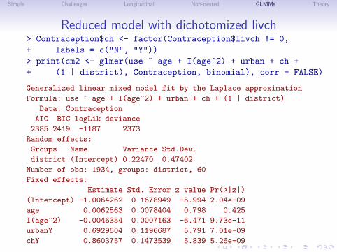
Simple Challenges Longitudinal Non-nested GLMMs Theory
Reduced model with dichotomized livch> Contraception$ch <- factor(Contraception$livch != 0,+ labels = c("N", "Y"))> print(cm2 <- glmer(use ~ age + I(age^2) + urban + ch ++ (1 | district), Contraception, binomial), corr = FALSE)
Generalized linear mixed model fit by the Laplace approximation
Formula: use ~ age + I(age^2) + urban + ch + (1 | district)
Data: Contraception
AIC BIC logLik deviance
2385 2419 -1187 2373
Random effects:
Groups Name Variance Std.Dev.
district (Intercept) 0.22470 0.47402
Number of obs: 1934, groups: district, 60
Fixed effects:
Estimate Std. Error z value Pr(>|z|)
(Intercept) -1.0064262 0.1678949 -5.994 2.04e-09
age 0.0062563 0.0078404 0.798 0.425
I(age^2) -0.0046354 0.0007163 -6.471 9.73e-11
urbanY 0.6929504 0.1196687 5.791 7.01e-09
chY 0.8603757 0.1473539 5.839 5.26e-09
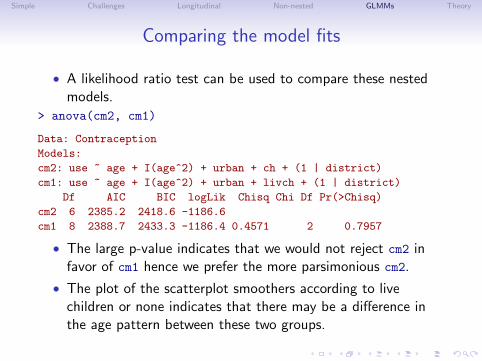
Simple Challenges Longitudinal Non-nested GLMMs Theory
Comparing the model fits
• A likelihood ratio test can be used to compare these nestedmodels.
> anova(cm2, cm1)
Data: Contraception
Models:
cm2: use ~ age + I(age^2) + urban + ch + (1 | district)
cm1: use ~ age + I(age^2) + urban + livch + (1 | district)
Df AIC BIC logLik Chisq Chi Df Pr(>Chisq)
cm2 6 2385.2 2418.6 -1186.6
cm1 8 2388.7 2433.3 -1186.4 0.4571 2 0.7957
• The large p-value indicates that we would not reject cm2 infavor of cm1 hence we prefer the more parsimonious cm2.
• The plot of the scatterplot smoothers according to livechildren or none indicates that there may be a difference inthe age pattern between these two groups.
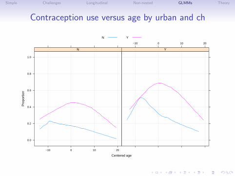
Simple Challenges Longitudinal Non-nested GLMMs Theory
Contraception use versus age by urban and ch
Centered age
Pro
port
ion
0.0
0.2
0.4
0.6
0.8
1.0
−10 0 10 20
N
−10 0 10 20
Y
N Y
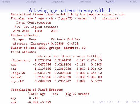
Simple Challenges Longitudinal Non-nested GLMMs Theory
Allowing age pattern to vary with chGeneralized linear mixed model fit by the Laplace approximation
Formula: use ~ age * ch + I(age^2) + urban + (1 | district)
Data: Contraception
AIC BIC logLik deviance
2379 2418 -1183 2365
Random effects:
Groups Name Variance Std.Dev.
district (Intercept) 0.22306 0.4723
Number of obs: 1934, groups: district, 60
Fixed effects:
Estimate Std. Error z value Pr(>|z|)
(Intercept) -1.3233174 0.2144470 -6.171 6.79e-10
age -0.0472956 0.0218394 -2.166 0.0303
chY 1.2107856 0.2069938 5.849 4.93e-09
I(age^2) -0.0057572 0.0008358 -6.888 5.64e-12
urbanY 0.7140326 0.1202579 5.938 2.89e-09
age:chY 0.0683522 0.0254347 2.687 0.0072
Correlation of Fixed Effects:
(Intr) age chY I(g^2) urbanY
age 0.719
chY -0.883 -0.793
I(age^2) -0.090 0.303 -0.101
urbanY -0.248 -0.076 0.118 -0.024
age:chY -0.596 -0.930 0.678 -0.498 0.071
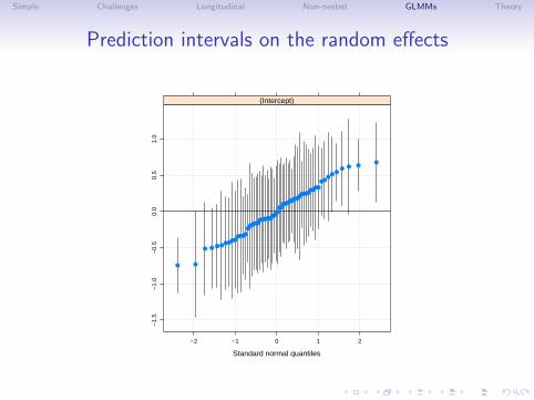
Simple Challenges Longitudinal Non-nested GLMMs Theory
Prediction intervals on the random effects
Standard normal quantiles
−1.
5−
1.0
−0.
50.
00.
51.
0
−2 −1 0 1 2
● ●
● ● ● ●●●●●
●●●●
●●●●●●
●●●●●●●●●
●●●●
●●●●●●●●●●●●●●
●●●●
●●●
●●
● ● ●●
(Intercept)
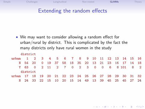
Simple Challenges Longitudinal Non-nested GLMMs Theory
Extending the random effects
• We may want to consider allowing a random effect forurban/rural by district. This is complicated by the fact themany districts only have rural women in the study
district
urban 1 2 3 4 5 6 7 8 9 10 11 12 13 14 15 16
N 54 20 0 19 37 58 18 35 20 13 21 23 16 17 14 18
Y 63 0 2 11 2 7 0 2 3 0 0 6 8 101 8 2
district
urban 17 18 19 20 21 22 23 24 25 26 27 28 29 30 31 32
N 24 33 22 15 10 20 15 14 49 13 39 45 25 45 27 24
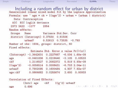
Simple Challenges Longitudinal Non-nested GLMMs Theory
Including a random effect for urban by districtGeneralized linear mixed model fit by the Laplace approximation
Formula: use ~ age * ch + I(age^2) + urban + (urban | district)
Data: Contraception
AIC BIC logLik deviance
2372 2422 -1177 2354
Random effects:
Groups Name Variance Std.Dev. Corr
district (Intercept) 0.37830 0.61506
urbanY 0.52613 0.72535 -0.793
Number of obs: 1934, groups: district, 60
Fixed effects:
Estimate Std. Error z value Pr(>|z|)
(Intercept) -1.3442631 0.2227667 -6.034 1.60e-09
age -0.0461836 0.0219446 -2.105 0.03533
chY 1.2116527 0.2082372 5.819 5.93e-09
I(age^2) -0.0056514 0.0008431 -6.703 2.04e-11
urbanY 0.7902095 0.1600484 4.937 7.92e-07
age:chY 0.0664682 0.0255674 2.600 0.00933
Correlation of Fixed Effects:
(Intr) age chY I(g^2) urbanY
age 0.696
chY -0.855 -0.792
I(age^2) -0.091 0.301 -0.097
urbanY -0.370 -0.061 0.088 -0.018
age:chY -0.575 -0.930 0.676 -0.496 0.055
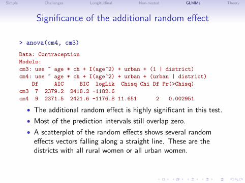
Simple Challenges Longitudinal Non-nested GLMMs Theory
Significance of the additional random effect
> anova(cm4, cm3)
Data: Contraception
Models:
cm3: use ~ age * ch + I(age^2) + urban + (1 | district)
cm4: use ~ age * ch + I(age^2) + urban + (urban | district)
Df AIC BIC logLik Chisq Chi Df Pr(>Chisq)
cm3 7 2379.2 2418.2 -1182.6
cm4 9 2371.5 2421.6 -1176.8 11.651 2 0.002951
• The additional random effect is highly significant in this test.
• Most of the prediction intervals still overlap zero.
• A scatterplot of the random effects shows several randomeffects vectors falling along a straight line. These are thedistricts with all rural women or all urban women.
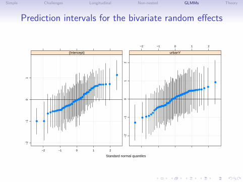
Simple Challenges Longitudinal Non-nested GLMMs Theory
Prediction intervals for the bivariate random effects
Standard normal quantiles
−2
−1
01
−2 −1 0 1 2
● ●
●●
● ●●●●●●●●●
●●●●●●●●●●
●●●●●●
●●●●●●●
●●●●●●
●●●●●
●●●●●●
● ● ● ● ●
●
(Intercept)
−2 −1 0 1 2
−2
−1
01
2●
●● ●
●●
●●
●●●●●●●●●●●●●●
●●●●●●●
●●●●●
●●●●●●●●●●●●●
●●●●●●●● ● ●●
●
●
urbanY
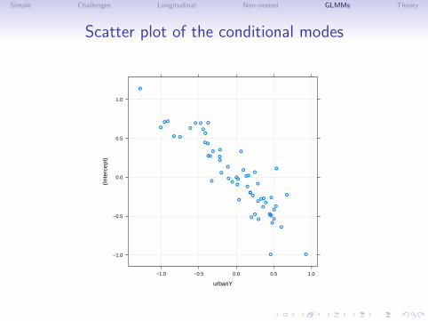
Simple Challenges Longitudinal Non-nested GLMMs Theory
Scatter plot of the conditional modes
urbanY
(Int
erce
pt)
−1.0
−0.5
0.0
0.5
1.0
−1.0 −0.5 0.0 0.5 1.0
●
●●
●
●
●
●
●
●
●
●
●
●
●
●
●
●
●●
●
●
●
●
●
●
●
●
● ●
●
●
●
●
●
●
●
●
●
●
●
●
● ●
●
●
●
●
●
●
●●
●
●●
●
●
●
●●●
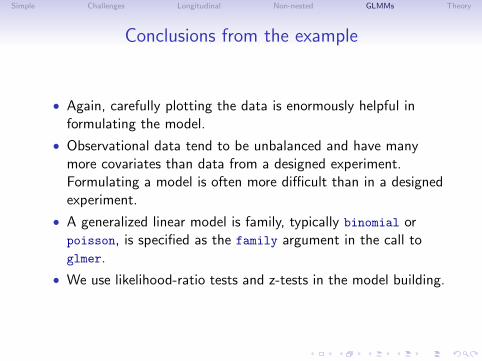
Simple Challenges Longitudinal Non-nested GLMMs Theory
Conclusions from the example
• Again, carefully plotting the data is enormously helpful informulating the model.
• Observational data tend to be unbalanced and have manymore covariates than data from a designed experiment.Formulating a model is often more difficult than in a designedexperiment.
• A generalized linear model is family, typically binomial orpoisson, is specified as the family argument in the call toglmer.
• We use likelihood-ratio tests and z-tests in the model building.
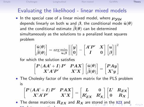
Simple Challenges Longitudinal Non-nested GLMMs Theory
Evaluating the likelihood - linear mixed models• In the special case of a linear mixed model, where µY|U
depends linearly on both u and β, the conditional mode u(θ)and the conditional estimate β(θ) can be determinedsimultaneously as the solutions to a penalized least squaresproblem[
u(θ)β(θ)
]= arg min
u,β
∥∥∥∥[y0
]−
[A′P ′ X
I 0
] [uβ
]∥∥∥∥2
for which the solution satisfies[P (AA′ + I) P ′ PAX
X ′A′P ′ X ′X
] [u(θ)β(θ)
]=
[PAyX ′y
]• The Cholesky factor of the system matrix for the PLS problem
is[P (AA′ + I) P ′ PAX
X ′A′P ′ X ′X
]=
[L 0
R′ZX R′
X
] [L′ RZX
0 RX
]• The dense matrices RZX and RX are stored in the RZX andRX slots, respectively.
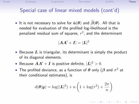
Simple Challenges Longitudinal Non-nested GLMMs Theory
Special case of linear mixed models (cont’d)
• It is not necessary to solve for u(θ) and β(θ). All that isneeded for evaluation of the profiled log-likelihood is thepenalized residual sum of squares, r2, and the determinant
|AA′ + I| = |L|2
• Because L is triangular, its determinant is simply the productof its diagonal elements.
• Because AA′ + I is positive definite, |L|2 > 0.
• The profiled deviance, as a function of θ only (β and σ2 attheir conditional estimates), is
d(θ|y) = log(|L|2) + n
(1 + log(r2) +
2π
n
)
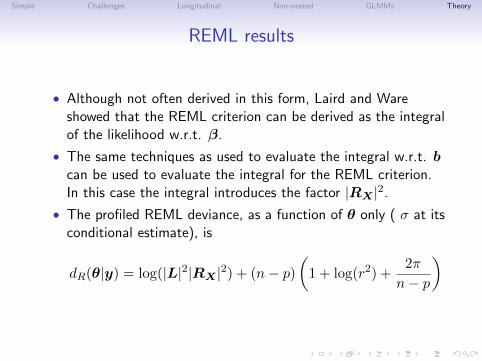
Simple Challenges Longitudinal Non-nested GLMMs Theory
REML results
• Although not often derived in this form, Laird and Wareshowed that the REML criterion can be derived as the integralof the likelihood w.r.t. β.
• The same techniques as used to evaluate the integral w.r.t. bcan be used to evaluate the integral for the REML criterion.In this case the integral introduces the factor |RX |2.
• The profiled REML deviance, as a function of θ only ( σ at itsconditional estimate), is
dR(θ|y) = log(|L|2|RX |2) + (n− p)(
1 + log(r2) +2π
n− p
)
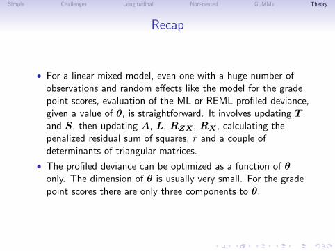
Simple Challenges Longitudinal Non-nested GLMMs Theory
Recap
• For a linear mixed model, even one with a huge number ofobservations and random effects like the model for the gradepoint scores, evaluation of the ML or REML profiled deviance,given a value of θ, is straightforward. It involves updating Tand S, then updating A, L, RZX , RX , calculating thepenalized residual sum of squares, r and a couple ofdeterminants of triangular matrices.
• The profiled deviance can be optimized as a function of θonly. The dimension of θ is usually very small. For the gradepoint scores there are only three components to θ.
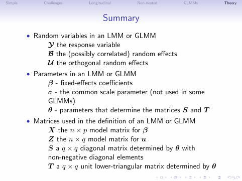
Simple Challenges Longitudinal Non-nested GLMMs Theory
Summary
• Random variables in an LMM or GLMMY the response variableB the (possibly correlated) random effectsU the orthogonal random effects
• Parameters in an LMM or GLMMβ - fixed-effects coefficientsσ - the common scale parameter (not used in someGLMMs)θ - parameters that determine the matrices S and T
• Matrices used in the definition of an LMM or GLMMX the n× p model matrix for βZ the n× q model matrix for uS a q × q diagonal matrix determined by θ withnon-negative diagonal elementsT a q × q unit lower-triangular matrix determined by θ