Mixed models in R using the lme4 package Part 4: Theory of ...lme4.r-forge.r-project.org/slides/2011-01-11-Madison/4Theory.pdf · Mixed models in R using the lme4 package Part 4:

Mixed models in R using the lme4 packagePart 4: Theory of linear mixed models

Douglas Bates

Department of StatisticsUniversity of Wisconsin - Madison

<[email protected]>

MadisonJanuary 11, 2011

Douglas Bates (Stat. Dept.) Theory of LMMs Jan. 11, 2011 1 / 26

Outline

1 Definition of linear mixed models

2 The penalized least squares problem

3 The sparse Cholesky factor

4 Evaluating the likelihood


Outline






Outline






Outline






Definition of linear mixed models

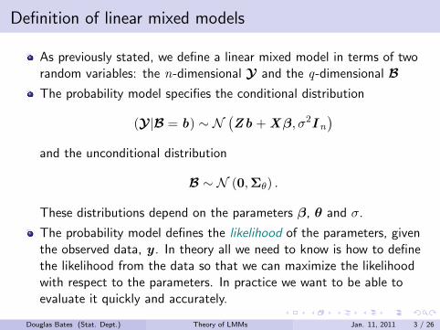
As previously stated, we define a linear mixed model in terms of tworandom variables: the n-dimensional Y and the q-dimensional BThe probability model specifies the conditional distribution

(Y |B = b) ∼ N(Zb +Xβ, σ2I n

)and the unconditional distribution

B ∼ N (0,Σθ) .

These distributions depend on the parameters β, θ and σ.

The probability model defines the likelihood of the parameters, giventhe observed data, y . In theory all we need to know is how to definethe likelihood from the data so that we can maximize the likelihoodwith respect to the parameters. In practice we want to be able toevaluate it quickly and accurately.


Properties of Σθ; generating it

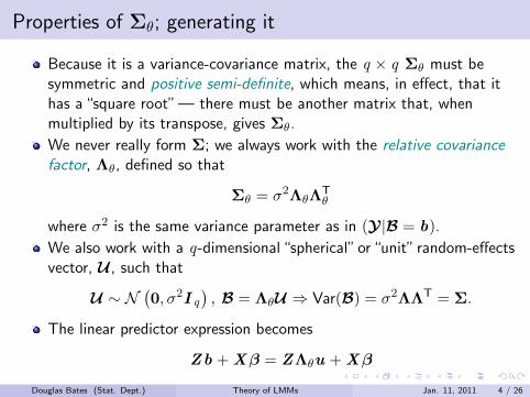
Because it is a variance-covariance matrix, the q × q Σθ must besymmetric and positive semi-definite, which means, in effect, that ithas a “square root” — there must be another matrix that, whenmultiplied by its transpose, gives Σθ.

We never really form Σ; we always work with the relative covariancefactor, Λθ, defined so that

Σθ = σ2ΛθΛTθ

where σ2 is the same variance parameter as in (Y |B = b).

We also work with a q-dimensional “spherical” or “unit” random-effectsvector, U , such that

U ∼ N(0, σ2I q

), B = ΛθU ⇒ Var(B) = σ2ΛΛT = Σ.

The linear predictor expression becomes

Zb +Xβ = ZΛθu +Xβ


The conditional mean µU |Y

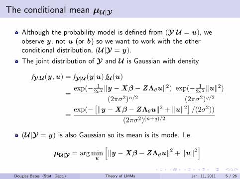
Although the probability model is defined from (Y |U = u), weobserve y , not u (or b) so we want to work with the otherconditional distribution, (U |Y = y).

The joint distribution of Y and U is Gaussian with density

fY,U (y ,u) = fY|U (y |u) fU (u)

=exp(− 1

2σ2 ‖y −Xβ − ZΛθu‖2)(2πσ2)n/2

exp(− 12σ2 ‖u‖2)

(2πσ2)q/2

=exp(−

[‖y −Xβ − ZΛθu‖2 + ‖u‖2

]/(2σ2))

(2πσ2)(n+q)/2

(U |Y = y) is also Gaussian so its mean is its mode. I.e.

µU |Y = argminu

[‖y −Xβ − ZΛθu‖2 + ‖u‖2

]Douglas Bates (Stat. Dept.) Theory of LMMs Jan. 11, 2011 5 / 26

Minimizing a penalized sum of squared residuals

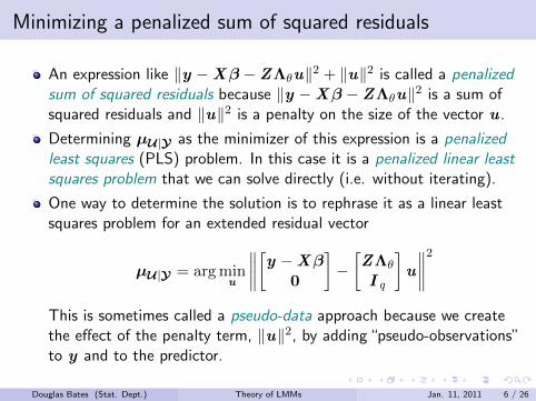
An expression like ‖y −Xβ − ZΛθu‖2 + ‖u‖2 is called a penalizedsum of squared residuals because ‖y −Xβ − ZΛθu‖2 is a sum ofsquared residuals and ‖u‖2 is a penalty on the size of the vector u .

Determining µU |Y as the minimizer of this expression is a penalizedleast squares (PLS) problem. In this case it is a penalized linear leastsquares problem that we can solve directly (i.e. without iterating).

One way to determine the solution is to rephrase it as a linear leastsquares problem for an extended residual vector

µU |Y = argminu

∥∥∥∥[y −Xβ0

]−[ZΛθ

I q

]u

∥∥∥∥2This is sometimes called a pseudo-data approach because we createthe effect of the penalty term, ‖u‖2, by adding “pseudo-observations”to y and to the predictor.


Solving the linear PLS problem

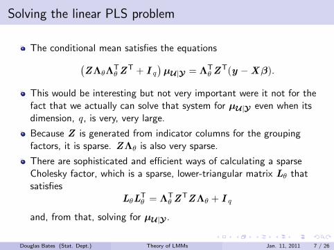
The conditional mean satisfies the equations(ZΛθΛ

Tθ Z

T + I q

)µU |Y = ΛT

θ ZT(y −Xβ).

This would be interesting but not very important were it not for thefact that we actually can solve that system for µU |Y even when itsdimension, q , is very, very large.

Because Z is generated from indicator columns for the groupingfactors, it is sparse. ZΛθ is also very sparse.

There are sophisticated and efficient ways of calculating a sparseCholesky factor, which is a sparse, lower-triangular matrix Lθ thatsatisfies

LθLTθ = ΛT

θ ZTZΛθ + I q

and, from that, solving for µU |Y .


The sparse Choleksy factor, Lθ

Because the ability to evaluate the sparse Cholesky factor, Lθ, is thekey to the computational methods in the lme4 package, we considerthis in detail.

In practice we will evaluate Lθ for many different values of θ whendetermining the ML or REML estimates of the parameters.

As described in Davis (2006), §4.6, the calculation is performed intwo steps: in the symbolic decomposition we determine the positionof the nonzeros in L from those in ZΛθ then, in the numericdecomposition, we determine the numerical values in those positions.Although the numeric decomposition may be done dozens, perhapshundreds of times as we iterate on θ, the symbolic decomposition isonly done once.


A fill-reducing permutation, P

In practice it can be important while performing the symbolicdecomposition to determine a fill-reducing permutation, which iswritten as a q × q permutation matrix, P . This matrix is just are-ordering of the columns of I q and has an orthogonality property,PPT = PTP = I q .

When P is used, the factor Lθ is defined to be the sparse,lower-triangular matrix that satisfies

LθLTθ = P

[ΛTθ Z

Tθ ZΛθ + I q

]PT

In the Matrix package for R, the Cholesky method for a sparse,symmetric matrix (class dsCMatrix) performs both the symbolic andnumeric decomposition. By default, it determines a fill-reducingpermutation, P . The update method for a Cholesky factor (classCHMfactor) performs the numeric decomposition only.


Applications to models with simple, scalar random effects

Recall that, for a model with simple, scalar random-effects terms only,the matrix Σθ is block-diagonal in k blocks and the ith block isσ2i I ni where ni is the number of levels in the ith grouping factor.

The matrix Λθ is also block-diagonal with the ith block being θiI ni ,where θi = σi/σ.

Given the grouping factors for the model and a value of θ we produceZΛθ then L, using Cholesky the first time then update.

To avoid recalculating we assign

flist a list of the grouping factorsnlev number of levels in each factorZt the transpose of the model matrix, Z

theta current value of θLambda current Λθ

Ut transpose of ZΛθ


Cholesky factor for the Penicillin model

> flist <- subset(Penicillin , select = c(plate , sample ))

> Zt <- do.call(rBind , lapply(flist , as, "sparseMatrix"))

> (nlev <- sapply(flist , function(f) length(levels(factor(f)))))

plate sample

24 6

> theta <- c(1.2, 2.1)

> Lambda <- Diagonal(x = rep.int(theta , nlev))

> Ut <- crossprod(Lambda , Zt)

> str(L <- Cholesky(tcrossprod(Ut), LDL = FALSE , Imult = 1))

Formal class ’dCHMsimpl’ [package "Matrix"] with 10 slots

..@ x : num [1:189] 3.105 0.812 0.812 0.812 0.812 ...

..@ p : int [1:31] 0 7 14 21 28 35 42 49 56 63 ...

..@ i : int [1:189] 0 24 25 26 27 28 29 1 24 25 ...

..@ nz : int [1:30] 7 7 7 7 7 7 7 7 7 7 ...

..@ nxt : int [1:32] 1 2 3 4 5 6 7 8 9 10 ...

..@ prv : int [1:32] 31 0 1 2 3 4 5 6 7 8 ...

..@ colcount: int [1:30] 7 7 7 7 7 7 7 7 7 7 ...

..@ perm : int [1:30] 23 22 21 20 19 18 17 16 15 14 ...

..@ type : int [1:4] 2 1 0 1

..@ Dim : int [1:2] 30 30Douglas Bates (Stat. Dept.) Theory of LMMs Jan. 11, 2011 11 / 26

Images of ΛTθZ

TZΛθ + I and L

Λ'Z'ZΛ + I

5

10

15

20

25

5 10 15 20 25

L

5

10

15

20

25

5 10 15 20 25

−4

−2

0

2

4

6

8

10

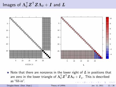
Note that there are nonzeros in the lower right of L in positions thatare zero in the lower triangle of ΛT

θ ZTZΛθ + I q . This is described

as “fill-in”.Douglas Bates (Stat. Dept.) Theory of LMMs Jan. 11, 2011 12 / 26

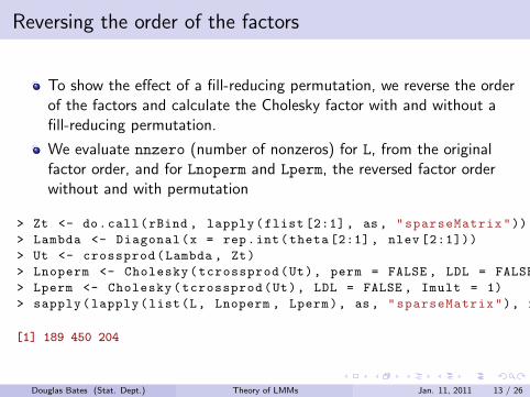
Reversing the order of the factors

To show the effect of a fill-reducing permutation, we reverse the orderof the factors and calculate the Cholesky factor with and without afill-reducing permutation.

We evaluate nnzero (number of nonzeros) for L, from the originalfactor order, and for Lnoperm and Lperm, the reversed factor orderwithout and with permutation

> Zt <- do.call(rBind , lapply(flist [2:1], as, "sparseMatrix"))

> Lambda <- Diagonal(x = rep.int(theta [2:1], nlev [2:1]))


> Lnoperm <- Cholesky(tcrossprod(Ut), perm = FALSE , LDL = FALSE , Imult = 1)

> Lperm <- Cholesky(tcrossprod(Ut), LDL = FALSE , Imult = 1)

> sapply(lapply(list(L, Lnoperm , Lperm), as , "sparseMatrix"), nnzero)

[1] 189 450 204


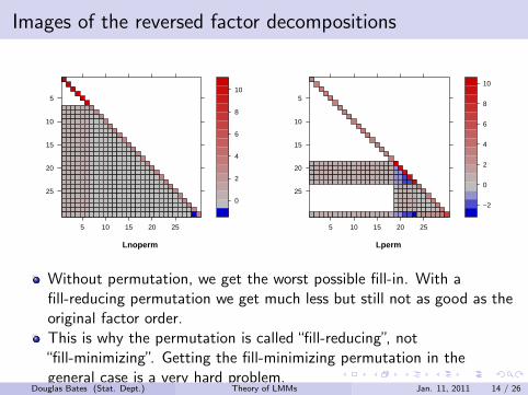
Images of the reversed factor decompositions

Lnoperm

5

10

15

20

25

5 10 15 20 25

0

2

4

6

8

10

Lperm

5

10

15

20

25

5 10 15 20 25

−2

0

2

4

6

8

10

Without permutation, we get the worst possible fill-in. With afill-reducing permutation we get much less but still not as good as theoriginal factor order.This is why the permutation is called “fill-reducing”, not“fill-minimizing”. Getting the fill-minimizing permutation in thegeneral case is a very hard problem.


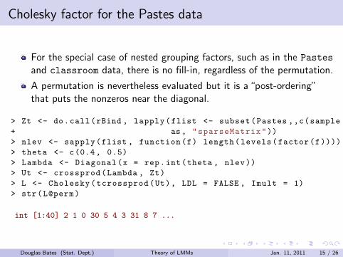
Cholesky factor for the Pastes data

For the special case of nested grouping factors, such as in the Pastes

and classroom data, there is no fill-in, regardless of the permutation.

A permutation is nevertheless evaluated but it is a “post-ordering”that puts the nonzeros near the diagonal.

> Zt <- do.call(rBind , lapply(flist <- subset(Pastes ,,c(sample , batch)),

+ as, "sparseMatrix"))

> nlev <- sapply(flist , function(f) length(levels(factor(f))))

> theta <- c(0.4, 0.5)

> Lambda <- Diagonal(x = rep.int(theta , nlev))


> L <- Cholesky(tcrossprod(Ut), LDL = FALSE , Imult = 1)

> str(L@perm)

int [1:40] 2 1 0 30 5 4 3 31 8 7 ...


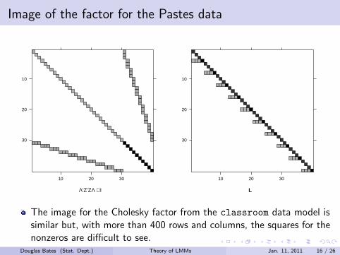
Image of the factor for the Pastes data

Λ'Z'ZΛ + I

10

20

30

10 20 30

L

10

20

30

10 20 30

The image for the Cholesky factor from the classroom data model issimilar but, with more than 400 rows and columns, the squares for thenonzeros are difficult to see.


The conditional density, fU |Y

We know the joint density, fY,U (y ,u), and

fU |Y(u |y) =fY,U (y ,u)∫fY,U (y ,u) du

so we almost have fU |Y . The trick is evaluating the integral in thedenominator, which, it turns out, is exactly the likelihood,L(θ,β, σ2|y), that we want to maximize.

The Cholesky factor, Lθ is the key to doing this because

PTLθLTθPµU |Y = ΛT

θ ZT(y −Xβ).

Although the Matrix package provides a one-step solve method forthis, we write it in stages:

Solve Lcu = PΛTθ Z

T(y −Xβ) for cu .Solve LTPµ = cu for PµU |Y and µU |Y as PTPµU |Y .


Evaluating the likelihood

The exponent of fY,U (y ,u) can now be written

‖y −Xβ − ZΛθu‖2 + ‖u‖2 = r2(θ,β) + ‖LTP(u − µU |Y)‖2.

where r2(θ,β) = ‖y −Xβ −UµU |Y‖2 + ‖µU |Y‖2. The first termdoesn’t depend on u and the second is relatively easy to integrate.

Use the change of variable v = LTP(u − µU |Y), withdv = abs(|L||P |) du , in

∫ exp

(−‖LTP(u−µU|Y )‖2

2σ2

)(2πσ2)q/2

du

=

∫ exp(−‖v‖22σ2

)(2πσ2)q/2

dv

abs(|L||P |)=

1

abs(|L||P |)=

1

|L|

because abs |P | = 1 and abs |L|, which is the product of its diagonalelements, all of which are positive, is positive.


Evaluating the likelihood (cont’d)

As is often the case, it is easiest to write the log-likelihood. On thedeviance scale (negative twice the log-likelihood)`(θ,β, σ|y) = logL(θ,β, σ|y) becomes

−2`(θ,β, σ|y) = n log(2πσ2) +r2(θ,β)

σ2+ log(|Lθ|2)

We wish to minimize the deviance. Its dependence on σ isstraightforward. Given values of the other parameters, we canevaluate the conditional estimate

σ̂2(θ,β) =r2(θ,β)

n

producing the profiled deviance

−2˜̀(θ,β|y) = log(|Lθ|2) + n

[1 + log

(2πr2(θ,β)

n

)]However, an even greater simplification is possible because thedeviance depends on β only through r2(θ,β).


Profiling the deviance with respect to β

Because the deviance depends on β only through r2(θ,β) we canobtain the conditional estimate, β̂θ, by extending the PLS problem to

r2θ = minu ,β

[‖y −Xβ − ZΛθu‖2 + ‖u‖2

]with the solution satisfying the equations[

ΛTθ Z

TZΛθ + I q U TθX

XTZΛθ XTX

] [µU |Yβ̂θ

]=

[ΛTθ Z

Ty

XTy .

]The profiled deviance, which is a function of θ only, is

−2˜̀(θ) = log(|Lθ|2) + n

[1 + log

(2πr2θn

)]


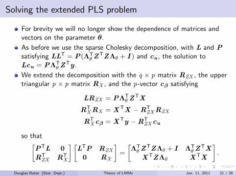
Solving the extended PLS problem

For brevity we will no longer show the dependence of matrices andvectors on the parameter θ.

As before we use the sparse Cholesky decomposition, with L and Psatisfying LLT = P(ΛT

θ ZTZΛθ + I ) and cu , the solution to

Lcu = PΛTθ Z

Ty .

We extend the decomposition with the q × p matrix RZX , the uppertriangular p × p matrix RX , and the p-vector cβ satisfying

LRZX = PΛTθ Z

TX

RTXRX = XTX −RT

ZXRZX

RTX cβ = XTy −RT

ZX cu

so that[PTL 0

RTZX RT

X

] [LTP RZX

0 RX

]=

[ΛTθ Z

TZΛθ + I ΛTθ Z

TX

XTZΛθ XTX

].


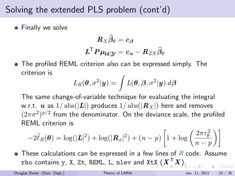
Solving the extended PLS problem (cont’d)

Finally we solve

RX β̂θ = cβ

LTPµU |Y = cu −RZX β̂θ

The profiled REML criterion also can be expressed simply. Thecriterion is

LR(θ, σ2|y) =

∫L(θ,β, σ2|y) dβ

The same change-of-variable technique for evaluating the integralw.r.t. u as 1/ abs(|L|) produces 1/ abs(|RX |) here and removes(2πσ2)p/2 from the denominator. On the deviance scale, the profiledREML criterion is

−2˜̀R(θ) = log(|L|2) + log(|Rx |2) + (n − p)

[1 + log

(2πr2θn − p

)]These calculations can be expressed in a few lines of R code. Assumerho contains y, X, Zt, REML, L, nlev and XtX (XTX ).


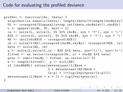
Code for evaluating the profiled deviance

profDev <- function(rho , theta) {

stopifnot(is.numeric(theta), length(theta )== length(rho$nlev))

Ut <- crossprod(Diagonal(x=rep.int(theta ,rho$nlev)),rho$Zt)

L <- update(rho$L, Ut, mult = 1)

cu <- solve(L, solve(L, Ut %*% rho$y, sys = "P"), sys = "L")

RZX <- solve(L, solve(L, Ut %*% rho$X, sys = "P"), sys = "L")

RX <- chol(rho$XtX - crossprod(RZX))

cb <- solve(t(RX),crossprod(rho$X,rho$y)- crossprod(RZX , cu))

beta <- solve(RX, cb)

u <- solve(L,solve(L,cu - RZX %*% beta , sys="Lt"), sys="Pt")

fitted <- as.vector(crossprod(Ut, u) + rho$X %*% beta)

prss <- sum(c(rho$y - fitted , as.vector(u))^2)

n <- length(fitted ); p <- ncol(RX)

if (rho$REML) return(determinant(L)$mod +

2 * determinant(RX)$mod +

(n-p) * (1+log(2*pi*prss/(n-p))))

determinant(L)$mod + n * (1 + log(2*pi*prss/n))

}


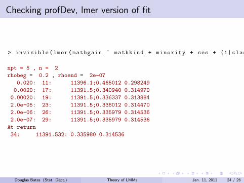
Checking profDev, lmer version of fit

> invisible(lmer(mathgain ~ mathkind + minority + ses + (1| classid) + (1| schoolid), classroom , verbose = 1, REML = FALSE))

npt = 5 , n = 2

rhobeg = 0.2 , rhoend = 2e-07

0.020: 11: 11396.1;0.465012 0.298249

0.0020: 17: 11391.5;0.340940 0.314970

0.00020: 19: 11391.5;0.336337 0.313884

2.0e-05: 23: 11391.5;0.336012 0.314470

2.0e-06: 26: 11391.5;0.335979 0.314536

2.0e-07: 29: 11391.5;0.335979 0.314536

At return

34: 11391.532: 0.335980 0.314536


How lmer works

Essentially lmer takes its arguments and creates a structure like therho environment shown above. The optimization of the profileddeviance or the profiled REML criterion happens within thisenvironment.

The creation of Λθ is somewhat more complex for models withvector-valued random effects but not excessively so.

Some care is taken to avoid allocating storage for large objects duringeach function evaluation. Many of the objects created in profDev areupdated in place within lmer.

Once the optimizer, bobyqa, has converged some additionalinformation for the summary is calculated.


Summary

For a linear mixed model, even one with a huge number ofobservations and random effects like the model for the grade pointscores, evaluation of the ML or REML profiled deviance, given a valueof θ, is straightforward. It involves updating Λθ, Lθ, RZX , RX ,calculating the penalized residual sum of squares, r2θ and twodeterminants of triangular matrices.

The profiled deviance can be optimized as a function of θ only. Thedimension of θ is usually very small. For the grade point scores thereare only three components to θ.


Documents

Mixed models in R using the lme4 package Part 4: Theory of ...lme4.r-forge.r-project.org/slides/2011-01-11-Madison/4Theory.pdf · Mixed models in R using the lme4 package Part 4: