Embed Size (px)
Citation preview

Introduction Choice of distributions to fit Fit of distributions Simulation of uncertainty Conclusion
Fitting parametric distributions using R: thefitdistrplus package
M. L. Delignette-Muller - CNRS UMR 5558R. Pouillot
J.-B. Denis - INRA MIAJ
useR! 2009,10/07/2009
Introduction Choice of distributions to fit Fit of distributions Simulation of uncertainty Conclusion
Background
Specifying the probability distribution that best fits a sampledata among a predefined family of distributions
a frequent need especially in Quantitative RiskAssessmentgeneral-purpose maximum-likelihood fitting routine for theparameter estimation step : fitdistr(MASS) (Venablesand Ripley, 2002)possibility to implement other steps using R (Ricci, 2005)but no specific package dedicated to the whole processdifficulty to work with censored data
Introduction Choice of distributions to fit Fit of distributions Simulation of uncertainty Conclusion
Objective
Build a package that provides functions to help the wholeprocess of specification of a distribution from data
choose among a family of distributions the best candidatesto fit a sampleestimate the distribution parameters and their uncertaintyassess and compare the goodness-of-fit of severaldistributions
that specifically handles different kinds of datadiscretecontinuous with possible censored values (right-, left- andinterval-censored with several upper and lower bounds)
Introduction Choice of distributions to fit Fit of distributions Simulation of uncertainty Conclusion
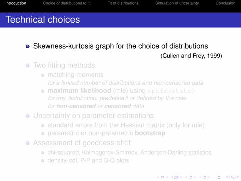
Technical choices
Skewness-kurtosis graph for the choice of distributions(Cullen and Frey, 1999)
Two fitting methodsmatching momentsfor a limited number of distributions and non-censored datamaximum likelihood (mle) using optim(stats)for any distribution, predefined or defined by the userfor non-censored or censored data
Uncertainty on parameter estimationsstandard errors from the Hessian matrix (only for mle)parametric or non-parametric bootstrap
Assessment of goodness-of-fitchi-squared, Kolmogorov-Smirnov, Anderson-Darling statisticsdensity, cdf, P-P and Q-Q plots
Introduction Choice of distributions to fit Fit of distributions Simulation of uncertainty Conclusion
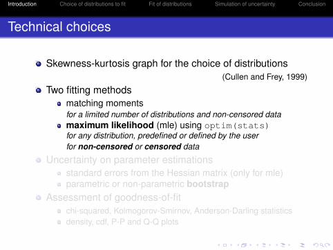
Technical choices
Skewness-kurtosis graph for the choice of distributions(Cullen and Frey, 1999)
Two fitting methodsmatching momentsfor a limited number of distributions and non-censored datamaximum likelihood (mle) using optim(stats)for any distribution, predefined or defined by the userfor non-censored or censored data
Uncertainty on parameter estimationsstandard errors from the Hessian matrix (only for mle)parametric or non-parametric bootstrap
Assessment of goodness-of-fitchi-squared, Kolmogorov-Smirnov, Anderson-Darling statisticsdensity, cdf, P-P and Q-Q plots
Introduction Choice of distributions to fit Fit of distributions Simulation of uncertainty Conclusion
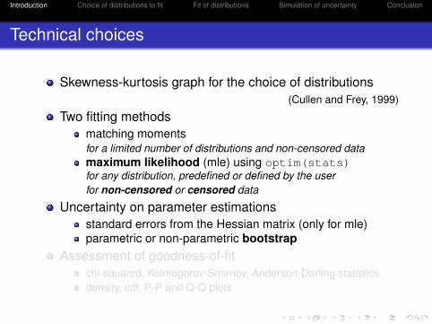
Technical choices
Skewness-kurtosis graph for the choice of distributions(Cullen and Frey, 1999)
Two fitting methodsmatching momentsfor a limited number of distributions and non-censored datamaximum likelihood (mle) using optim(stats)for any distribution, predefined or defined by the userfor non-censored or censored data
Uncertainty on parameter estimationsstandard errors from the Hessian matrix (only for mle)parametric or non-parametric bootstrap
Assessment of goodness-of-fitchi-squared, Kolmogorov-Smirnov, Anderson-Darling statisticsdensity, cdf, P-P and Q-Q plots
Introduction Choice of distributions to fit Fit of distributions Simulation of uncertainty Conclusion
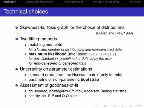
Technical choices
Skewness-kurtosis graph for the choice of distributions(Cullen and Frey, 1999)
Two fitting methodsmatching momentsfor a limited number of distributions and non-censored datamaximum likelihood (mle) using optim(stats)for any distribution, predefined or defined by the userfor non-censored or censored data
Uncertainty on parameter estimationsstandard errors from the Hessian matrix (only for mle)parametric or non-parametric bootstrap
Assessment of goodness-of-fitchi-squared, Kolmogorov-Smirnov, Anderson-Darling statisticsdensity, cdf, P-P and Q-Q plots
Introduction Choice of distributions to fit Fit of distributions Simulation of uncertainty Conclusion
Main functions of fitdistrplus
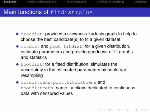
descdist: provides a skewness-kurtosis graph to help tochoose the best candidate(s) to fit a given datasetfitdist and plot.fitdist: for a given distribution,estimate parameters and provide goodness-of-fit graphsand statisticsbootdist: for a fitted distribution, simulates theuncertainty in the estimated parameters by bootstrapresamplingfitdistcens, plot.fitdistcens andbootdistcens: same functions dedicated to continuousdata with censored values
Introduction Choice of distributions to fit Fit of distributions Simulation of uncertainty Conclusion
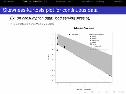
Skewness-kurtosis plot for continuous dataEx. on consumption data: food serving sizes (g)> descdist(serving.size)
●
0 1 2 3 4
Cullen and Frey graph
square of skewness
kurt
osis
109
87
65
43
21 ● Observation Theoretical distributions
normaluniformexponentiallogistic
betalognormalgamma
(Weibull is close to gamma and lognormal)
●
Introduction Choice of distributions to fit Fit of distributions Simulation of uncertainty Conclusion
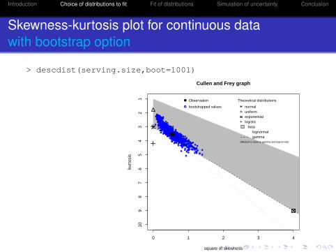
Skewness-kurtosis plot for continuous datawith bootstrap option
> descdist(serving.size,boot=1001)
●
0 1 2 3 4
Cullen and Frey graph
square of skewness
kurt
osis
109
87
65
43
21 ● Observation
● bootstrapped values
Theoretical distributions
normaluniformexponentiallogistic
betalognormalgamma
(Weibull is close to gamma and lognormal)
●
●
●
●
●
●
●
●
●
●
●
●
●
●
●
●
●
●
●
● ●
●
●
●
●
●
●
●
●
●
●
●
●
●●●
●
●
●
●● ●
●
● ●●
●●
●
●
●●
●●
●
● ●
●
●
●
●
●
●
●
●
●
●
●●
●
●
●
●
●
●
●
●
●
●
●●
●
● ●
●
●
●
●
●
●
●●
●
●
●
●
●
●
●
●
●
●
●
●
●
●
●
● ●
●
●
●
●
●
●
●●
●
●
●
●
●
●
●
●
●
●
●
●
●
●
●
●
●
●
●
●
●
●
●
●
● ●
●
●
●
●
●
●
●
●
●●
●
●
●
●
●
●
●
●●
●
●
●
●
●
●
●
●
● ●
●
●
●●
●
●
●
●
●
●
●
●
●
●
●
●
●
●
●
●
●
●
●
●
●
●
●
●
●
●
●●
●
●
●
●
●
●
●
●
●●
●
●
●
●
●
●
● ●●●
●
●
●
●
●
●
●
●
●●
●
●
●●
●●
●
●
●
●●
●●
●
●
●
●
●
●
●
●●
●
●
●● ●
●
●
●
●
●
●
●
●
●
●
●
●
●
●
●
●
●
●
●
●
●
●
●
●
●
●
●
●
●
●
●●
●
●
●
●●
●
●
●●
●
●
●
●
●
●
●●
●
●
●
●
●
●
●
●
●
●
●
●
●
●
●
●
●
●
●
●
●
●
●
●
●
●
●
●●
●
●●●
●
●
● ●
●
●
●
●
●
●
●●
●●●
●
●●
●●
●
●
●
●
●
●
●
●
●
●
●
●
●
●
●●●
●
●
●
●
●
●
●
●
●
●
●
●
●
●
●
●
●
● ●
●
●
●●
●●
●
● ●
●●
●
●
●
●
●
●
●
●
●
●
●
●●
●●
●
●
●
●
●
●
●
●
●
●
●● ●
●
●
●
●
●
●
●
●
●
●
●●
●
●
●
●
●
●
●
●
●
●
●●●
●
●
●
●
●
●
●
●
●
●
●
●
●
●
●●
●
● ●
●
●
●
●
●
● ●
●
●
●
●
●
●
●
●
●
●
●●
●
●
●
●●
●
●
●
●
●
●
●
●
●
●
●
●
●
●
●
●
●
●
●
●
● ●
●
●
●
●
●
●
●
●
●
●
●
●
●
●
●
●
●
●
●
●
●●
●
●
●
●●
●
●
●
●
●
●
●
●
●
●
●●
●
●
●
●●
●
●
●●
●
●●
●
●
●
●
●
●
●
●
●
●
●
●
●
●
●
●●
●
●●
●
●
●
●
●
●
●
●
● ●
●
●
●
●
●●
●
●
●
●
●
●
●
●
●
●
●
●
●
●
●
●
●
●
●
●
●
●
●
●
●
●
●●
●
●
●
●
●
●
●
●
●
●
●
●
●
●
●
●
●
●
●
●
●●
●
●
●
●
●
●
●
●
●
●
●
●
●
●
●
●
●
●
●
●
●
●
●●
●
●
●
●
●
●
●
●
●
●
●
●
●
●
●
●
●
●
●
●
●
●
●
●
●
●
●
●
● ●
●
●
●
●
●●
●
●
●●
● ●
●
●
●●
●
●
●
●
●
●●
●
●
●
●
●
●
●
●
●
● ●
●●
●
●
●
●
●
●
●
●
●
●●
●
●●
●
●
●
●
●
●
●
●
●
●
●●
●
●
●
●●
●●
●
●
●
●
●
●
●
●
●
●
●
●
●●
●
●●
●
●
●
●
●
●
●
●
●●
●
●
●
●●
●
●
●●
●
●●
● ●
●
●
● ●
●●
●
●
●●
●
●
● ●
●●
● ●
●
●
●●
●
●
●
●
●
●●
●●
●
●
●
●●●
●
●
●
●
●
●
●
●
●
●
●
●
●
●
●
●
●
●●
●
●
●
●
●
●
●
●
●
●
●
●
●
●
●
●
● ●
●
●
●●
●
●
●
●
●
●
●
●
●
●
●
●
●
●
●
●
●●●
●
●
●
● ●
●
●
●
●
●●
●
●
●●
●
●
●
●
●
●●
●
●
●
●●
●●
●
●
●
●
●
●
●
●●
●
●
●
●
●
●
●
●
●
●
●
●
●
●
●
●
● ●
●
●
●
●●
● ●
●
●
●
●
●
●
●
●
●
●
●
●
Introduction Choice of distributions to fit Fit of distributions Simulation of uncertainty Conclusion
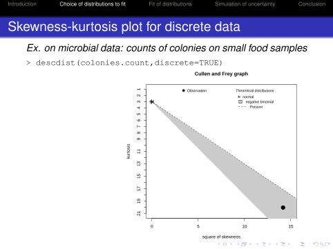
Skewness-kurtosis plot for discrete dataEx. on microbial data: counts of colonies on small food samples> descdist(colonies.count,discrete=TRUE)
●
0 5 10 15
Cullen and Frey graph
square of skewness
kurt
osis
2119
1715
1311
98
76
54
32
1 ● Observation Theoretical distributions
normalnegative binomial
Poisson
●

Introduction Choice of distributions to fit Fit of distributions Simulation of uncertainty Conclusion
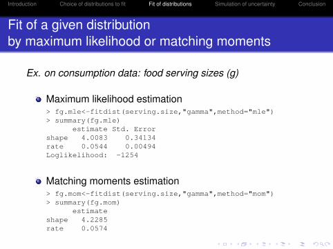
Fit of a given distributionby maximum likelihood or matching moments
Ex. on consumption data: food serving sizes (g)
Maximum likelihood estimation> fg.mle<-fitdist(serving.size,"gamma",method="mle")> summary(fg.mle)
estimate Std. Errorshape 4.0083 0.34134rate 0.0544 0.00494Loglikelihood: -1254
Matching moments estimation> fg.mom<-fitdist(serving.size,"gamma",method="mom")> summary(fg.mom)
estimateshape 4.2285rate 0.0574
Introduction Choice of distributions to fit Fit of distributions Simulation of uncertainty Conclusion
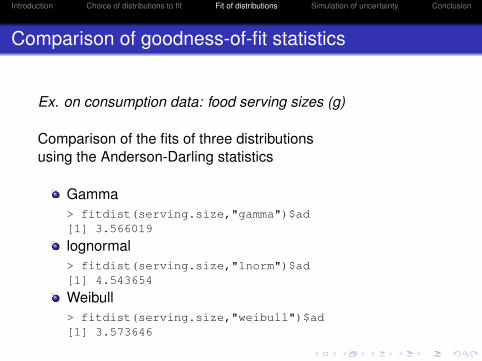
Comparison of goodness-of-fit statistics
Ex. on consumption data: food serving sizes (g)
Comparison of the fits of three distributionsusing the Anderson-Darling statistics
Gamma> fitdist(serving.size,"gamma")$ad[1] 3.566019
lognormal> fitdist(serving.size,"lnorm")$ad[1] 4.543654
Weibull> fitdist(serving.size,"weibull")$ad[1] 3.573646
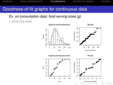
Introduction Choice of distributions to fit Fit of distributions Simulation of uncertainty Conclusion
Goodness-of-fit graphs for continuous dataEx. on consumption data: food serving sizes (g)> plot(fg.mle)
Empirical and theoretical distr.
data
Den
sity
0 50 100 150 2000.
000
0.00
40.
008
0.01
2
●●●●●●●●●●●
●●●●●●●●●●●●●●●●●●●●●●●●●●●●●●●●●●●●●●
●●●●●●●●●●●●●●●●●●●●●●●●●●●●●●●●●●●●●●●●●●●●●●●●●●●●●●●●●●●●●●●●●●●●●●●●●●●●●●●●●●●●●●●●●●●●●●●●●●●●●●●●●●●●●●●●●●●●●●●●●●●●●●●●●●●●●●
●●●●●●●●●●●●●●●●●●●●
●●●●●●●●●●●●●●●●●●●●●●●●●●●●●●●●●●●●●●●●●●●●
●●●●
● ● ●
50 100 150 200
5010
015
020
0
QQ−plot
theoretical quantiles
sam
ple
quan
tiles
0 50 100 150 200
0.0
0.2
0.4
0.6
0.8
1.0
Empirical and theoretical CDFs
data
CD
F
●●●●●●●●●●●●●
●●●●●●●●●●●●●●●●●
●●●●●●●●●●●●●●●●●● ●
●●●●●●●●●●●●●●●●●●●●●●●●●●●●●●●●●●●●●●●●●●●●●●●●●●●●●●●●●●●●●
●●●●●● ●● ●●● ●●●●● ●●●
●●●●●●●●●●●●●●●●●●●●●●●●●●●●●●●●●●●●●●●●●●●●●●●●●●●●●● ●
●●●●●●●●●●●●●●●●●●●●●●●●●●●●●●●● ●●●●●
●●●●●●●●●●●●●●●●●●●●●●●●●● ●●●●●●●
0.0 0.2 0.4 0.6 0.8 1.00.
00.
20.
40.
60.
81.
0
PP−plot
theoretical probabilities
sam
ple
prob
abili
ties
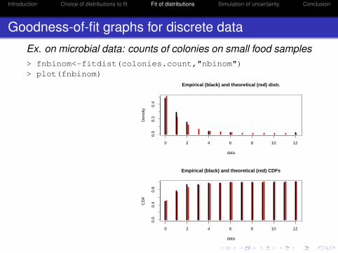
Introduction Choice of distributions to fit Fit of distributions Simulation of uncertainty Conclusion
Goodness-of-fit graphs for discrete dataEx. on microbial data: counts of colonies on small food samples> fnbinom<-fitdist(colonies.count,"nbinom")> plot(fnbinom)
0 2 4 6 8 10 12
0.0
0.2
0.4
Empirical (black) and theoretical (red) distr.
data
Den
sity
0 2 4 6 8 10 12
0.0
0.4
0.8
Empirical (black) and theoretical (red) CDFs
data
CD
F

Introduction Choice of distributions to fit Fit of distributions Simulation of uncertainty Conclusion
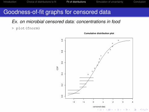
Fit of a given distributionby maximum likelihood to censored data
Ex. on microbial censored data: concentrations in foodwith left censored values (not detected)and interval censored values (detected but not counted)
> log10.concleft right
1 1.73 1.732 1.51 1.513 0.77 0.774 1.96 1.965 1.96 1.966 -1.40 0.007 -1.40 -0.708 NA -1.409 -0.11 -0.11...
> fnorm<-fitdistcens(log10.conc, "norm")> summary(fnorm)
estimate Std. Errormean 0.118 0.332sd 1.426 0.261
Loglikelihood: -32.1
Introduction Choice of distributions to fit Fit of distributions Simulation of uncertainty Conclusion
Goodness-of-fit graphs for censored dataEx. on microbial censored data: concentrations in food> plot(fnorm)
−2 −1 0 1 2 3 4
0.0
0.2
0.4
0.6
0.8
1.0
Cumulative distribution plot
censored data
CD
F
Introduction Choice of distributions to fit Fit of distributions Simulation of uncertainty Conclusion
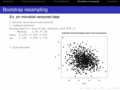
Bootstrap resamplingEx. on microbial censored data> bnorm<-bootdistcens(fnorm)> summary(bnorm)Nonparametric bootstrap medians and 95% CI
Median 2.5% 97.5%mean 0.233 -0.455 0.875sd 1.294 0.908 1.776
> plot(bnorm)
●
● ●
●
●
●
●
●
●
●
●
●
●
●
●
●
●
●
●
●
●
●
●
●
●
●
●
●
●
●
●
●
●
●
●
●
●●●
●
●
● ●
●
●●●
●
●
●
●
●
●
●●
●
●
●
●
●●
●
●
●
●
●
●
●
●
●
●
●
●
●
●
●
●
●
●
●
●
●
●
●
●
●
●
●
●
●
●
●
●
●
●
●●
●
●
●
●●
●
●
● ●
●
●
●
●
●
●
●
●
●
●
●
●
●
●
●●
●
●
●
●
●
●
●
●
●
●
●
●
●
●
●
●●
●
●
●
●
●
●●
●
●
●
●
●
●
●
●
●
●
●
●
●
●
●
●
●
●
●
●
●
●
●
●
●
●
●●
●
●
●
●
●
●
●●
●
●
●
●
●
●●
●
●
●
●
●
●
●
●●
●
●
●
●●
●
●
●
●
●
●
●
●
●
●●
●
●
●
●
●
●
●
●
●
●
●
●
●
●
●
●
●
●
●
●
●
●
●●
●
●
●●
●
●
●
●
●
●
●
●
●
●
●
●
●●
●
●
●
●●
●
●
●
●
●
●
●
●
●
●●
●
●
●
●●
●
●
●
●
●
●
●●
●
●
●
●
● ●
●●
●●
●
●
●
●
●
●
●
●
●
● ●
●
●●
●
●
●
●
●
●
●
●
●
●
●
●
●
●
●
●
●
●●
●
●
●
●
●
●
●
●
●●
●
●
●
●
● ●
●
●
●
●●
●
●●
●
●
●
●
●
●
●
●●
●●
●
●
●
●
●
●
●
●
●
●
●
●
●
●●
●
●
●
●
●
●
●
●
●
●●
●
●
●●
●
●
●
●
●
●●
●
●
●●
●
●
●
●
●
●
●
●
●
● ●
●
●
●
●
●
●
●
●
●
●
●
●●
●
●
●
● ●
●
●
●●
●
●
●
●
●
●
●
●
● ●
●
●
●
●●
●
●
●●
●
●
●
●
●
●
●
●
●
●
●●
●
●
●
●
●
●●
●
●
● ●
●
●
●
●
●
●
●
●
●
●
●●
●
●●
●
●
●
●
●
●
●
●
●
●
●
●●
●
●
●
●
●
●
●
●
●
●
●
●
●
●
●
●
●
●
●
●
●
●
●
●
● ●
●
●
●
●
●
●
●
●
●
●
●
●
●
●
●
●●
●
●
●
●
●
●
●
●
●
●
●
●
●
●
●
●
●
●
●
● ●
●
●
●
●
●
●
●
●
●
●
●
●
●
●
●
●
●
●
●
●
●
●
●
●
●
●
●
●
●
●
●
●
●
●
●
●
●●
●●
●
●
●
●
●
●
●
●
●
●
●
●
●
●
●
●
●
●
●
●●
●
●
●
●
●
●
●
●
●
●
●●
●●
●
●
●
●
●
●
●
●
●
●
●
●●
●
●
●●
●
●●●
●
●
●
●
●
●
●
●●
●
●●
●
●
●
●
●
●
●●
●
●
●
●
●
●
●
●
●
●
●
●
●
●
●
●
●
●
●●
●
●
●
●
●
●
●
●
●●●
●
●
●
●
●
●
●
●
●
●
●
●
●
●
●
●
●
●
●
●●
●
●
●●
●
●
●
●●
●
●
●●
●
●
●
●
●
●
●
●
●
●
●
●
●
●
●
●
●
●
●
●
●● ●
●
●●
●
●
●
●
●
●
●
● ●
●
●●
●●
●
●
●●
●
●
●
●
●
●●
●
● ●
●
●
●
●
●
●
●
●
●
●●
●
●
●
●●
●
●
●
●
●
●
●
●
●
●
●
●
●
●
●
●
●
●
●
●
●
●
●
●
●
●
●●
●
●
●
●
●
●
●
●
●
●
●
●
●
●
●
●●
●
●
●
● ●
●
●
●
●
●
●
●
●
●
●
●
●
●
●
●●
●
●
●●
●
●
●
●
●
●
●
●
●
●
●●
●
●
●●
●
●
●
●
●
●
●
●●
●
●
●
●
●
●
●
●
●
●
●
●●
●
●
●
●
●
●
●
●
●
●●
●
●
●
●
●
●
●
●
●
●
●
●
●
●
●
●
●
●
●
●
●
●
●
●
●
●
●
●
●
●
●
●
●
●
●●
●
●
●
●
●
●
●
●
●
●
●
●
● ●
●
●
●
●
●
●●
●
−0.5 0.0 0.5 1.0
1.0
1.5
2.0
Scatterplot of the boostrapped values of the two parameters
mean
sd
Introduction Choice of distributions to fit Fit of distributions Simulation of uncertainty Conclusion
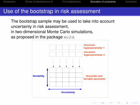
Use of the bootstrap in risk assessment
The bootstrap sample may be used to take into accountuncertainty in risk assessment,in two-dimensional Monte Carlo simulations,as proposed in the package mc2d.
Variability
Uncertainty
Uncertain and Variable parameter
Uncertain hyperparameter 1Uncertain hyperparameter 2
Introduction Choice of distributions to fit Fit of distributions Simulation of uncertainty Conclusion
Conclusion
fitdistrplus could help risk assessment.It is a part of a collaborative project with 2 other packagesunder development, mc2d and ReBaStaBa:
The R-Forge project "Risk Assessment with R"http://riskassessment.r-forge.r-project.org/
fitdistrplus could also be used more largely to helpthe fit of univariate distributions to data

Introduction Choice of distributions to fit Fit of distributions Simulation of uncertainty Conclusion
Still many things to do
fitdistrplus is still under development.Many improvements are planned
other goodness-of-fit statisticsother graphs for goodness-of-fit for censored data(Turnbull,...)optimized choice of the algorithm used in optim for thelikelihood maximizationgraphs of likelihood contours (detection of identifiabilityproblems)...
do not hesitate to provide us other improvement ideas !