Embed Size (px)
Citation preview

Student report
Eloy Rodríguez Moldes
Flexible load management inSmart-grids
Master Thesis for Msc Energy Technology
Project report, May 2013

Title: Flexible load management in Smart-gridsSemester: 10thSemester theme: Master ThesisProject period: 01.09.12 to 29.05.13ECTS: 50Supervisor: Pukar MahatProject group: WPS4-1052
Eloy Rodriguez Moldes
SYNOPSIS:
This report describes the implementationof a demand side management system ina residential area. A study on washingmachine and refrigerator operation is con-ducted, as well as the use pattern de-sign. The optimal control of the appli-ances is done using the Matlab Optimiza-tion Toolbox for the purpose of minimizingthe losses in the distribution lines, and thefinal price of the electrical energy for thecustomers. Finally the optimal operationpattern for the appliances is implementedin a model of the grid in DIgSILENT, tovalidate the line losses reduction an controlthe power quality.
Copies: 3Pages, total: 82Appendix: 14
By signing this document, the author confirms that he has participatedin the project work and thereby he is liable for the content of the report.


Preface
This Master Thesis project report, called Flexible load management in Smart-gridsis written by Eloy Rodríguez Moldes in the period 1th of September 2012 to 29thof May 2013.
Reading Instructions
• Figures are numbered sequentially in their own chapter. For example Figure1.3 is the third figure in the first chapter.
• Equations are numbered in the same way as figures but they are shown inbrackets.
• References are specified in the text in square parentheses according to Harvardmethod. The bibliography is on page 43.
i/vi


Acknowledgements
The author of this report would like to thank Pukar Mahat for his excellent guidanceas a supervisor for this project.
iii/vi

iv/vi
Contents
Preface i
Acknowledgements iii
Contents v
1 Introduction 1
1.1 Background . . . . . . . . . . . . . . . . . . . . . . . . . . . . . . . . 1
1.2 Solutions approach . . . . . . . . . . . . . . . . . . . . . . . . . . . . 3
1.3 Prior work in the field . . . . . . . . . . . . . . . . . . . . . . . . . . 3
1.4 Problem Statement . . . . . . . . . . . . . . . . . . . . . . . . . . . . 3
1.5 Key assumption and limitations . . . . . . . . . . . . . . . . . . . . . 4
2 Flexible loads 5
2.1 Introduction to Demand Side Management . . . . . . . . . . . . . . 5
2.1.1 DSM methods . . . . . . . . . . . . . . . . . . . . . . . . . . 7
2.2 Residential electricity demand . . . . . . . . . . . . . . . . . . . . . . 8
2.3 Study cases . . . . . . . . . . . . . . . . . . . . . . . . . . . . . . . . 10
3 Appliances 13
3.1 Washing Machine . . . . . . . . . . . . . . . . . . . . . . . . . . . . . 13
3.1.1 Use Pattern . . . . . . . . . . . . . . . . . . . . . . . . . . . . 16
3.2 Refrigerator . . . . . . . . . . . . . . . . . . . . . . . . . . . . . . . . 21
4 Optimization 25
4.1 Problem Formulation . . . . . . . . . . . . . . . . . . . . . . . . . . . 25
v/vi
4.2 Energy cost function . . . . . . . . . . . . . . . . . . . . . . . . . . . 27
4.3 Losses function . . . . . . . . . . . . . . . . . . . . . . . . . . . . . . 27
4.4 Optimization using Matlab Optimization Toolbox . . . . . . . . . . . 28
4.4.1 Constraints . . . . . . . . . . . . . . . . . . . . . . . . . . . . 28
4.4.2 Solver Functions . . . . . . . . . . . . . . . . . . . . . . . . . 29
4.5 Optimization results . . . . . . . . . . . . . . . . . . . . . . . . . . . 31
5 Modeling 35
5.1 System description . . . . . . . . . . . . . . . . . . . . . . . . . . . . 35
5.2 Implementation of optimal results . . . . . . . . . . . . . . . . . . . 35
5.3 Energy Losses . . . . . . . . . . . . . . . . . . . . . . . . . . . . . . . 38
6 Conclusion and future work 41
Bibliography 43
vi/vi

Chapter 1
Introduction
1.1 Background
According to the Energy Strategy 2050 of the Danish Ministry of Climate andEnergy, 30% of total electricity is to be covered by renewable energy consumptionby 2020.
During last years the Danish Power system has moved from a centralized modelsupported by large power production plants to a decentralized system. This changehas been motivated by the introduction of renewable energy resources like windand photovoltaic. However, the increases of this kind of generation facilities turninto in a stochastic energy supply system due to the high weather reliance.
One of the main problems in electricity networks, which becomes even bigger ingrids with large renewable resources, is the load balancing. The imbalance betweenelectricity production and consumption leads to the necessity of power plants withfast response (as CHP) and storage systems (as batteries), which are able to com-pensate random renewable generation. However, even with this solution, there isstill a need for the conventional power plants which should run during the periodof lower availability of renewable energy.
Other possibility is the actions on the demand side. The Demand Side Man-agement (DSM) is load profile variation in order to change the consumption withproduction. By this management, it is possible to shift electricity consumption withrespect to production or prices considerations, or both. Thereby, it is possible totake advantage of a possible prices policy with different time-variant tariff schemes.Various tariff schemes are discussed in detail in reference [1].
The adaptation to power production becomes of special interest in Smart-Gridswhere the energy available is not only limited, but also fluctuating. Furthermore,the energy efficiency can also be improved in large system with smart grid. Thatimprovement bases on more efficient distribution, since the consumption powerpeak decreases, and consequently the losses should decreases too. Besides, it ispossible to flatten the load profile, which leads to a better use and exploitation of
1/45

1.1. Background Introduction
the production systems, avoiding need of over-sizing.
Another use of DSM is the real-time response to fast variations on the produc-tion, which could be originated by wind gusts or any other stochastic generation.The dynamic response of thermal storage appliances as freezers and air conditioningcould help to manage these by frequency regulation.
The objective with DSM is not to decrease the amount of energy consumedat a dwelling, but to increase the utilization and efficiency of the production, andtransportation systems and decrease the total cost for the user [4].
2/45
1.2. Solutions approach
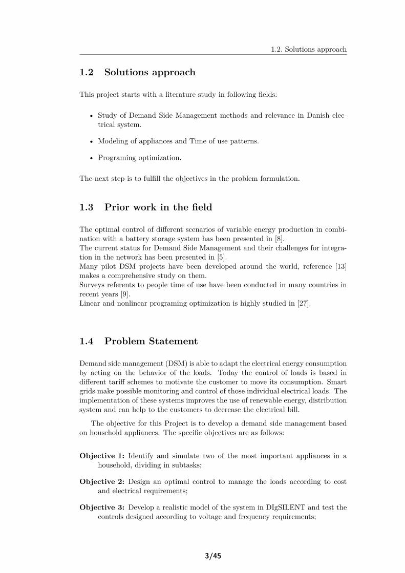
1.2 Solutions approach
This project starts with a literature study in following fields:
• Study of Demand Side Management methods and relevance in Danish elec-trical system.
• Modeling of appliances and Time of use patterns.
• Programing optimization.
The next step is to fulfill the objectives in the problem formulation.
1.3 Prior work in the field
The optimal control of different scenarios of variable energy production in combi-nation with a battery storage system has been presented in [8].The current status for Demand Side Management and their challenges for integra-tion in the network has been presented in [5].Many pilot DSM projects have been developed around the world, reference [13]makes a comprehensive study on them.Surveys referents to people time of use have been conducted in many countries inrecent years [9].Linear and nonlinear programing optimization is highly studied in [27].
1.4 Problem Statement
Demand side management (DSM) is able to adapt the electrical energy consumptionby acting on the behavior of the loads. Today the control of loads is based indifferent tariff schemes to motivate the customer to move its consumption. Smartgrids make possible monitoring and control of those individual electrical loads. Theimplementation of these systems improves the use of renewable energy, distributionsystem and can help to the customers to decrease the electrical bill.
The objective for this Project is to develop a demand side management basedon household appliances. The specific objectives are as follows:
Objective 1: Identify and simulate two of the most important appliances in ahousehold, dividing in subtasks;
Objective 2: Design an optimal control to manage the loads according to costand electrical requirements;
Objective 3: Develop a realistic model of the system in DIgSILENT and test thecontrols designed according to voltage and frequency requirements;
3/45
1.5. Key assumption and limitations
1.5 Key assumption and limitations
In order to simplify the calculations only active power is considered.Flexible pricing have not been considered.Calculations are based on the combination of UK time use survey, and data froma residential area in Denmark.The same washing program have been considered for all the washing machines.Refrigerator opening doors is not considered, and food mass is taken as a constantvalue.Communication infrastructure between utility company and final user is not con-sidered.
4/45
Chapter 2
Flexible loads
As mentioned before, the Danish Power System’s evolution has led to a decen-tralized power production scenario, contributing to significant power production ofrenewable resources. According to the annual report of the Danish Energy Agency,in 2011, the generation from RE was of 14% of the total energy production, andshows a growing trend in the use of this kind of energy.
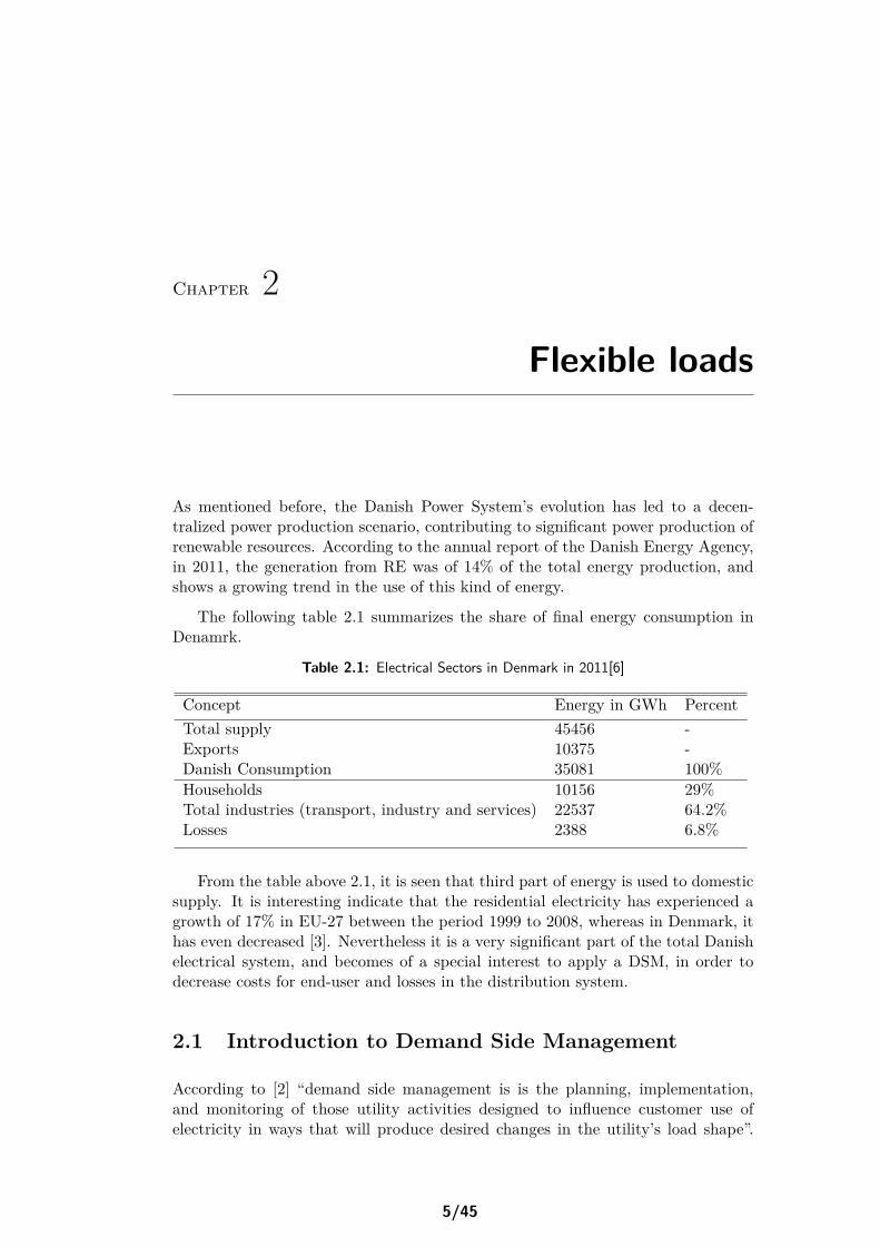
The following table 2.1 summarizes the share of final energy consumption inDenamrk.
Table 2.1: Electrical Sectors in Denmark in 2011[6]
Concept Energy in GWh PercentTotal supply 45456 -Exports 10375 -Danish Consumption 35081 100%Households 10156 29%Total industries (transport, industry and services) 22537 64.2%Losses 2388 6.8%
From the table above 2.1, it is seen that third part of energy is used to domesticsupply. It is interesting indicate that the residential electricity has experienced agrowth of 17% in EU-27 between the period 1999 to 2008, whereas in Denmark, ithas even decreased [3]. Nevertheless it is a very significant part of the total Danishelectrical system, and becomes of a special interest to apply a DSM, in order todecrease costs for end-user and losses in the distribution system.
2.1 Introduction to Demand Side Management
According to [2] “demand side management is is the planning, implementation,and monitoring of those utility activities designed to influence customer use ofelectricity in ways that will produce desired changes in the utility’s load shape”.
5/45
2.1. Introduction to Demand Side Management Flexible loads
This definition covers the reduction in total energy consumption, but also the loadshifting and customer generation, getting a more beneficial load profile. Thesebenefits include economical and efficiency improvements, from generation utilitiesas well as distribution system or final consumer. In general a DSM considers loadsable to react to external parameters. This consideration introduces the concept offlexible load with which, an utility will be able to adapt its consumption within acertain constraints.
The correct implementation of a DSM should maintain the same final servicesthat the electrical grid provides to the users today. However, it is also possible tochange the user habits, while maintaining the same comfort label.
In addiction, the security of supply is improved by DSM when renewable energysuch as wind or solar are used. These type of electrical generation is associated witha high temporal variability since it can not be reliably dispatched or accuratelypredicted. Due to this, match generation and consumption becomes of a specialinterest. A correct combination of valley filling and peak shaving could aid toreduce this problem.
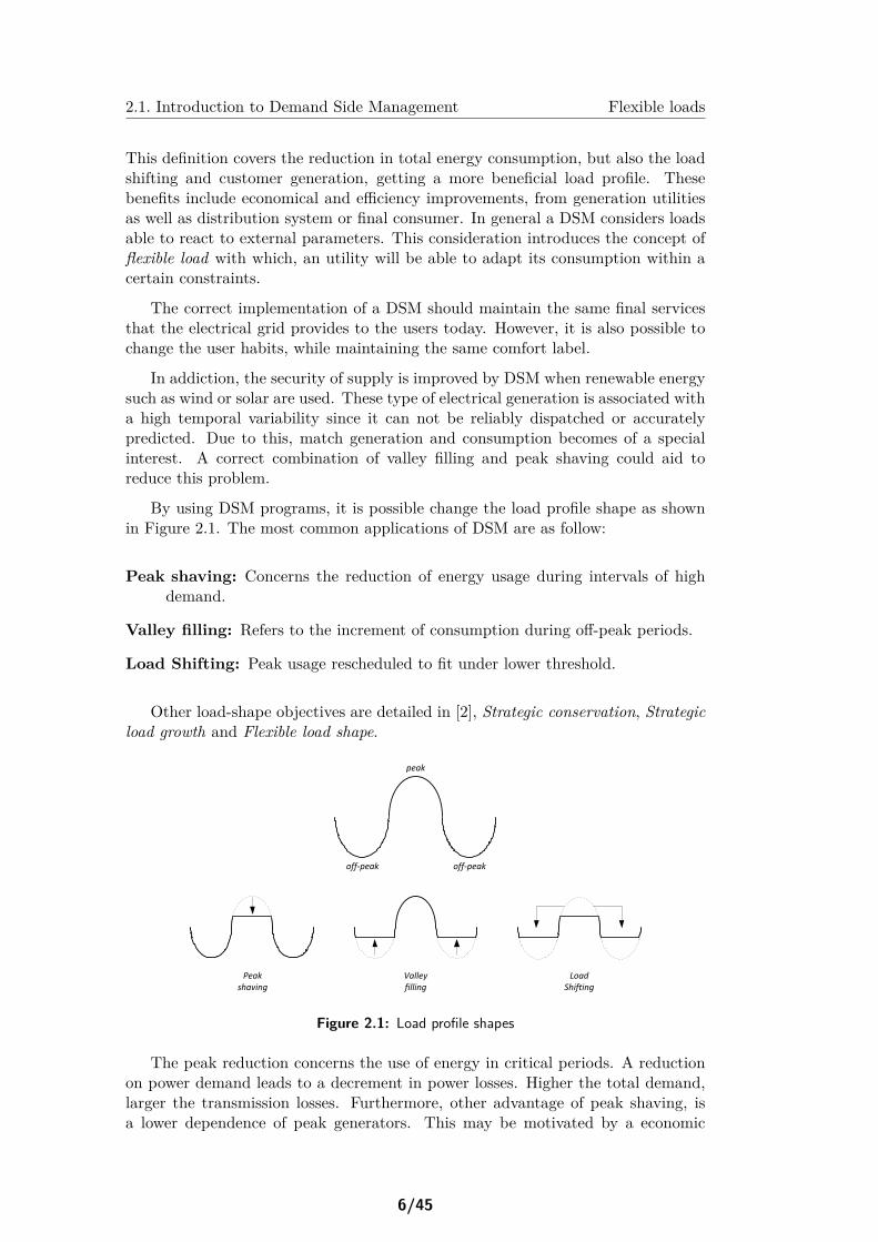
By using DSM programs, it is possible change the load profile shape as shownin Figure 2.1. The most common applications of DSM are as follow:
Peak shaving: Concerns the reduction of energy usage during intervals of highdemand.
Valley filling: Refers to the increment of consumption during off-peak periods.
Load Shifting: Peak usage rescheduled to fit under lower threshold.
Other load-shape objectives are detailed in [2], Strategic conservation, Strategicload growth and Flexible load shape.
off-peak off-peak
peak
Peak shaving
Valley filling
Load Shifting
Figure 2.1: Load profile shapes
The peak reduction concerns the use of energy in critical periods. A reductionon power demand leads to a decrement in power losses. Higher the total demand,larger the transmission losses. Furthermore, other advantage of peak shaving, isa lower dependence of peak generators. This may be motivated by a economic
6/45
Flexible loads 2.1. Introduction to Demand Side Management
reasons so as to, decrease the usually high operating costs and fuel dependence ofgenerators during critical periods.
A proper load management could help to flatten the load profile, avoiding ef-fects of intermittent generation and improving the efficiency of the system. Themodification of the load shape by increasing the consumption in off-peak periodsresults in a better use of base generators. In that periods, the cheap energy fromrenewable sources or from sources with high disconnection costs, such as nuclearpower plants, could be used.
DSM are intended to benefit both customers and suppliers. While the sup-pliers try to maximize profits by saving cost on production and distribution, thecustomers try to minimize invoice amount by using more efficient loads and adapt-ing consumption with a price schedule. In this report, both problems have beenconsidered. On one hand, the losses in the distribution line will be minimized byadjusting the loads and, on the other hand the cost of consumption will also beminimized by the rescheduling different process within some specific load.
2.1.1 DSM methods
The different methods of DSM are defined according to the interaction level betweenconsumer and supplier [10], some of the most common methods are summarizedbelow.
1. Energy saving and Load efficiency
It refers to efficiency improvements in electrical equipment, which results to areduction in energy consumption. New control is required once the new equipmenthas been installed. The effects on the electrical demand are indirect, since it focuseson power reduction regardless of consumption schedule.
2. Pricing models
It bases on energy regulation by means of price incentives. The main ideais the introduction of various energy prices at different periods during the day.The differences in price might be adequate both in quantity and time, to motivatecustomers to vary its consumption habits [1]. That prices can be established inadvance, for example in the energy supply contract, or it can be daily updated oreven in real time, basis on many parameters factors. Three of these managementsare briefly explained in next paragraphs.
Time of use tariff (TOU): This method is based on the definition of time blockswith different prices, which reflect the average energy cost during these peri-ods. For example lowest prices during the night.
Critical peak pricing (CPP): The high prices are allocated in periods wherethe generation cost is very high, usually due to a lack in generation or anexcessive consumption. The objective is to promote a peak shaving (Figure2.1).
Real time pricing (RTP): This kind of tariff reflects the variations in the mar-ket, usually in hourly periods. For example fluctuations in fuel price. This
7/45
2.2. Residential electricity demand
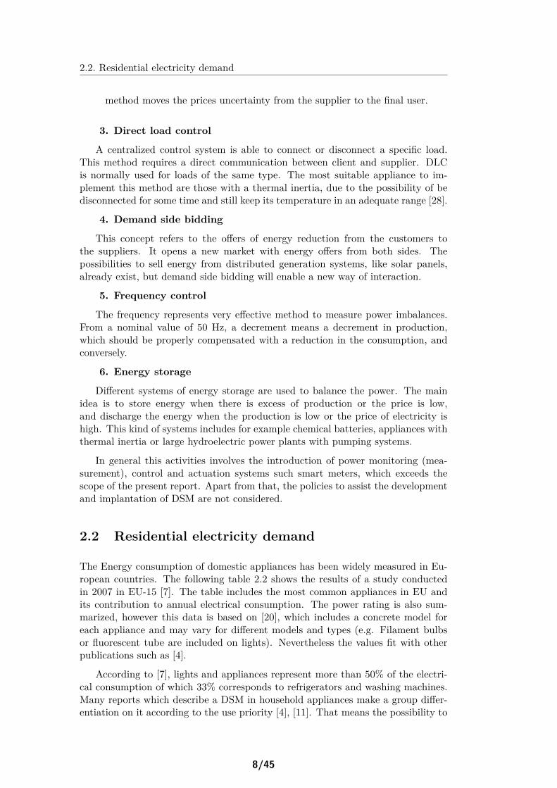
method moves the prices uncertainty from the supplier to the final user.
3. Direct load control
A centralized control system is able to connect or disconnect a specific load.This method requires a direct communication between client and supplier. DLCis normally used for loads of the same type. The most suitable appliance to im-plement this method are those with a thermal inertia, due to the possibility of bedisconnected for some time and still keep its temperature in an adequate range [28].
4. Demand side bidding
This concept refers to the offers of energy reduction from the customers tothe suppliers. It opens a new market with energy offers from both sides. Thepossibilities to sell energy from distributed generation systems, like solar panels,already exist, but demand side bidding will enable a new way of interaction.
5. Frequency control
The frequency represents very effective method to measure power imbalances.From a nominal value of 50 Hz, a decrement means a decrement in production,which should be properly compensated with a reduction in the consumption, andconversely.
6. Energy storage
Different systems of energy storage are used to balance the power. The mainidea is to store energy when there is excess of production or the price is low,and discharge the energy when the production is low or the price of electricity ishigh. This kind of systems includes for example chemical batteries, appliances withthermal inertia or large hydroelectric power plants with pumping systems.
In general this activities involves the introduction of power monitoring (mea-surement), control and actuation systems such smart meters, which exceeds thescope of the present report. Apart from that, the policies to assist the developmentand implantation of DSM are not considered.
2.2 Residential electricity demand
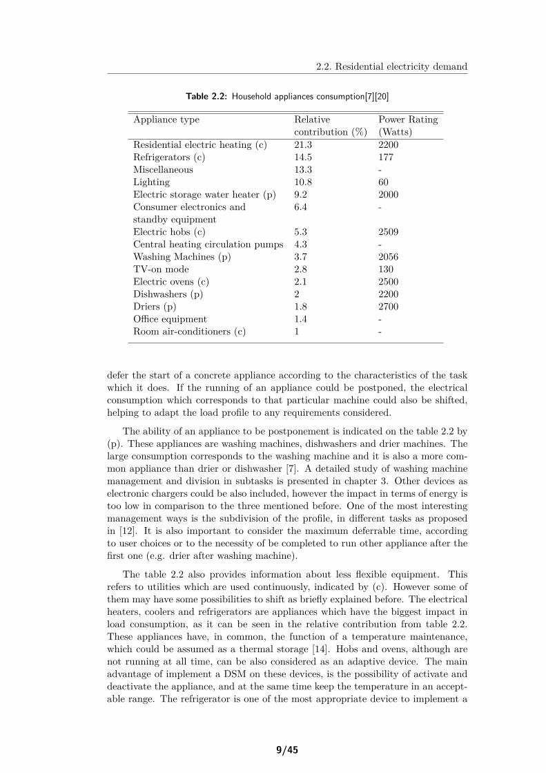
The Energy consumption of domestic appliances has been widely measured in Eu-ropean countries. The following table 2.2 shows the results of a study conductedin 2007 in EU-15 [7]. The table includes the most common appliances in EU andits contribution to annual electrical consumption. The power rating is also sum-marized, however this data is based on [20], which includes a concrete model foreach appliance and may vary for different models and types (e.g. Filament bulbsor fluorescent tube are included on lights). Nevertheless the values fit with otherpublications such as [4].
According to [7], lights and appliances represent more than 50% of the electri-cal consumption of which 33% corresponds to refrigerators and washing machines.Many reports which describe a DSM in household appliances make a group differ-entiation on it according to the use priority [4], [11]. That means the possibility to
8/45
2.2. Residential electricity demand
Table 2.2: Household appliances consumption[7][20]
Appliance type Relative Power Ratingcontribution (%) (Watts)
Residential electric heating (c) 21.3 2200Refrigerators (c) 14.5 177Miscellaneous 13.3 -Lighting 10.8 60Electric storage water heater (p) 9.2 2000Consumer electronics and 6.4 -standby equipmentElectric hobs (c) 5.3 2509Central heating circulation pumps 4.3 -Washing Machines (p) 3.7 2056TV-on mode 2.8 130Electric ovens (c) 2.1 2500Dishwashers (p) 2 2200Driers (p) 1.8 2700Office equipment 1.4 -Room air-conditioners (c) 1 -
defer the start of a concrete appliance according to the characteristics of the taskwhich it does. If the running of an appliance could be postponed, the electricalconsumption which corresponds to that particular machine could also be shifted,helping to adapt the load profile to any requirements considered.
The ability of an appliance to be postponement is indicated on the table 2.2 by(p). These appliances are washing machines, dishwashers and drier machines. Thelarge consumption corresponds to the washing machine and it is also a more com-mon appliance than drier or dishwasher [7]. A detailed study of washing machinemanagement and division in subtasks is presented in chapter 3. Other devices aselectronic chargers could be also included, however the impact in terms of energy istoo low in comparison to the three mentioned before. One of the most interestingmanagement ways is the subdivision of the profile, in different tasks as proposedin [12]. It is also important to consider the maximum deferrable time, accordingto user choices or to the necessity of be completed to run other appliance after thefirst one (e.g. drier after washing machine).
The table 2.2 also provides information about less flexible equipment. Thisrefers to utilities which are used continuously, indicated by (c). However some ofthem may have some possibilities to shift as briefly explained before. The electricalheaters, coolers and refrigerators are appliances which have the biggest impact inload consumption, as it can be seen in the relative contribution from table 2.2.These appliances have, in common, the function of a temperature maintenance,which could be assumed as a thermal storage [14]. Hobs and ovens, although arenot running at all time, can be also considered as an adaptive device. The mainadvantage of implement a DSM on these devices, is the possibility of activate anddeactivate the appliance, and at the same time keep the temperature in an accept-able range. The refrigerator is one of the most appropriate device to implement a
9/45
2.3. Study cases
DSM due to the relatively big range of temperatures for the food to be preserved.
The third group of appliances includes those that are not possible to shift, andany change in their power consumption profile could affect to its operation. Thisgroup includes appliances like lights, TV or some office equipment.
2.3 Study cases
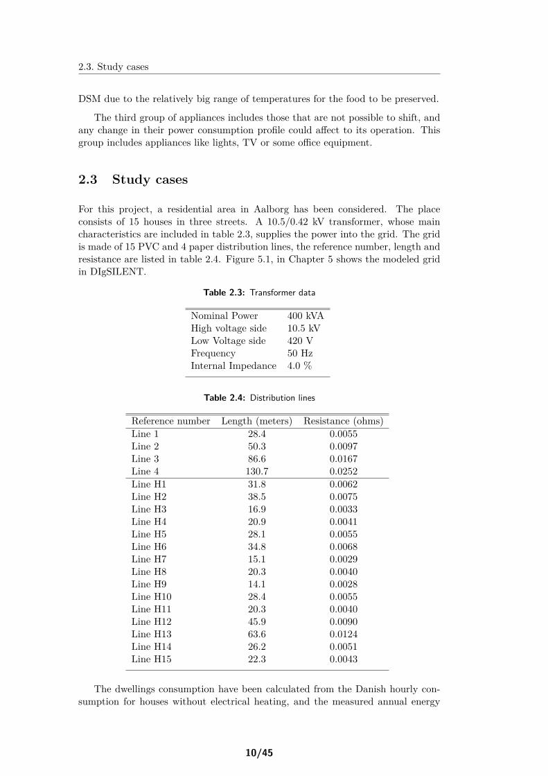
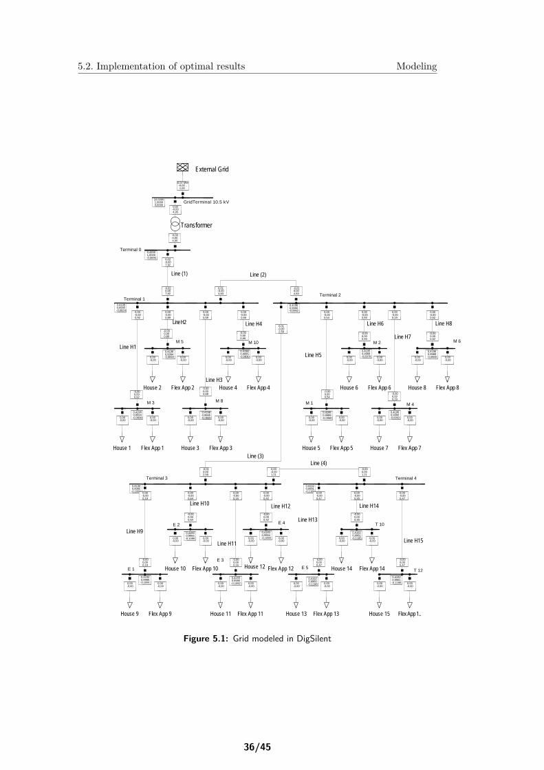
For this project, a residential area in Aalborg has been considered. The placeconsists of 15 houses in three streets. A 10.5/0.42 kV transformer, whose maincharacteristics are included in table 2.3, supplies the power into the grid. The gridis made of 15 PVC and 4 paper distribution lines, the reference number, length andresistance are listed in table 2.4. Figure 5.1, in Chapter 5 shows the modeled gridin DIgSILENT.
Table 2.3: Transformer data
Nominal Power 400 kVAHigh voltage side 10.5 kVLow Voltage side 420 VFrequency 50 HzInternal Impedance 4.0 %
Table 2.4: Distribution lines
Reference number Length (meters) Resistance (ohms)Line 1 28.4 0.0055Line 2 50.3 0.0097Line 3 86.6 0.0167Line 4 130.7 0.0252Line H1 31.8 0.0062Line H2 38.5 0.0075Line H3 16.9 0.0033Line H4 20.9 0.0041Line H5 28.1 0.0055Line H6 34.8 0.0068Line H7 15.1 0.0029Line H8 20.3 0.0040Line H9 14.1 0.0028Line H10 28.4 0.0055Line H11 20.3 0.0040Line H12 45.9 0.0090Line H13 63.6 0.0124Line H14 26.2 0.0051Line H15 22.3 0.0043
The dwellings consumption have been calculated from the Danish hourly con-sumption for houses without electrical heating, and the measured annual energy
10/45
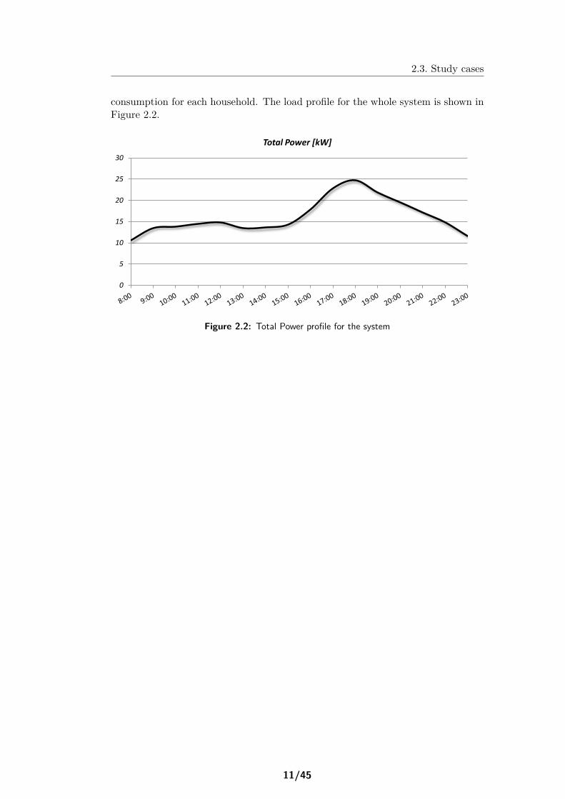
2.3. Study cases
consumption for each household. The load profile for the whole system is shown inFigure 2.2.
0
5
10
15
20
25
30
Total Power [kW]
Figure 2.2: Total Power profile for the system
11/45

2.3. Study cases
12/45

Chapter 3
Appliances
As explained before, two of the most appropriate appliances, in a household, forDSM according to the amount of energy consumption, are washing machines andrefrigerators. This chapter provides an analysis of both devices, in order to under-stand their operation and decide a correct management of flexible consumption.
3.1 Washing Machine
The first considered domestic appliance for DSM has been the washing machine.It is seen from the table 2.2 that the annual energy consumption of the washingmachine represents the largest among the deferrable appliances.
Basically, there are two different types of washing machines (horizontal axisand vertical axis) which have been produced by leading manufacturers for the lastyears. The main difference between them is the drum rotational axis direction.However, nowadays the vertical axis is not popular due to the biggest water andenergy consumption [15]. As a result of the low energy consumption, horizontalaxis is the most used in Europe and all the models considered as the most energyefficient household washing machines are with horizontal axis [16].
The basic design of a horizontal axis washing machine consists on an electricalmotor, connected to the drum where the laundry is washed, and a water heater.As it is explained in next paragraphs, during a wash cycle, high and fast variationsoccur in the drum. Thus it needs a motor capable of satisfying these requirements.One of the motors, which can be easily used to this purpose and also generally usedin washing machines is an induction motor [19] [17].
In a normal washing cycle, three different processes occur, wash mode, rinsemode and spin mode [18]. These mode are briefly explained in the next section inorder to get a better understanding of the washing process. These modes can bedifferent for each manufacturer and program.
13/45
3.1. Washing Machine Appliances
1. Wash mode
The objective of this mode is to remove the dirt of the laundry. The drum speedfor a wash mode is typically 30-45 rpm [17]. During this mode hot water is suppliedat the chosen temperature program. As it is shown in the load profile (Figure 3.3),the water heater increases the energy consumption compared to rinse and spinmodes, and it is the main energy consumer. The wash mode uses a small amountof water which generates high torque in the load when wet and heavy clothes dropfrom the drum’s highest point [17][18].
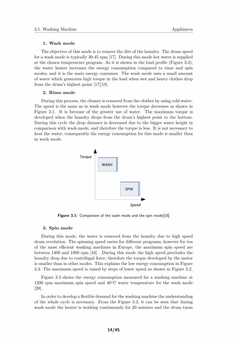
2. Rinse mode
During this process, the cleaner is removed from the clothes by using cold water.The speed is the same as in wash mode however the torque decreases as shown inFigure 3.1. It is because of the greater use of water. The maximum torque isdeveloped when the laundry drops from the drum’s highest point to the bottom.During this cycle the drop distance is decreased due to the bigger water height incomparison with wash mode, and therefore the torque is less. It is not necessary toheat the water; consequently the energy consumption for this mode is smaller thanin wash mode.
WASH
SPIN
Torque
Speed
Figure 3.1: Comparison of the wash mode and the spin mode[18]
3. Spin mode
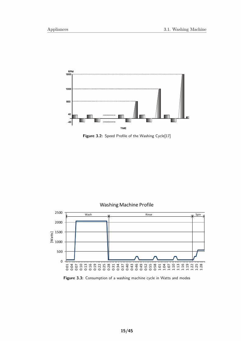
During this mode, the water is removed from the laundry due to high speeddrum revolution. The spinning speed varies for different programs, however for tenof the most efficient washing machines in Europe, the maximum spin speed arebetween 1400 and 1800 rpm [16] . During this mode the high speed precludes thelaundry drop due to centrifugal force, therefore the torque developed by the motoris smaller than in other modes. This explains the low energy consumption in Figure3.3. The maximum speed is raised by steps of lower speed as shown in Figure 3.2.
Figure 3.3 shows the energy consumption measured for a washing machine at1200 rpm maximum spin speed and 40◦C water temperature for the wash mode[20].
In order to develop a flexible demand for the washing machine the understandingof the whole cycle is necessary. From the Figure 3.3, it can be seen that duringwash mode the heater is working continuously for 20 minutes and the drum turns
14/45
Appliances 3.1. Washing Machine
Washing Machine Three-Phase AC-Induction Direct Vector Control, Rev.1
Washing Machine Algorithm
Freescale Semiconductor20
Figure 15. Speed Profile of the Washing Cycle
4.1 Tumble-Wash CycleThe tumble-wash phase is typical with low drum speeds reversing the direction of the drum rotation every few turns. Because there are short intervals of rotation, the drum must reach a stable rotational speed in under two seconds. This requirement necessitates applying a high torque to the washer drum to make it move. A high-generated torque is one of the key requirements in this operating mode. The speed of the drum for a tumble wash is typically 30–45 rpm. The exact speed depends on the type of clothes being washed and is determined by the washing program. The drum speed is low and the clothes rise in the drum and fall down when they reach the highest point. Wet and heavy clothes are periodically bumped in the drum, generating high torque ripples to the motor. The control algorithm of the drive needs to have enough dynamics to eliminate those ripples. Error in the speed should not exceed limits of ± 2 RPM. These requirements can be satisfied where there is a PID controller for a speed control loop and an inner PI current control loop.
4.2 Out-of-Balance DetectionThe out-of-balance detection and load displacement phase is performed prior to the washer going into a spin-dry. The clothes in the drum must be properly balanced to minimize centrifugal forces causing a waggling of the washer. In the first step, the imbalance is detected. The speed of the drum is increased by a ramp up to the value at which the clothes become centrifuged to the inner side of the drum. The algorithm performs an integration of the motor torque ripple per one cycle. The integral value estimates the size of the load imbalance. If the imbalance is lower than the safety limit, the drum speed increases and goes into a dry-spin. If the imbalance is higher than the safety limit, the drum speed decreases and the rotation direction is reversed. The algorithm performs a new load displacement at the reversed speed. At the end of a load displacement interval, the rotation is reversed and out-of-balance detection is executed again. The
40
600
-40
000
800RPM
TIME
40
600
-40
000
800RPM
TIME
Figure 3.2: Speed Profile of the Washing Cycle[17]
0
500
1000
1500
2000
2500
0:0
1
0:0
4
0:0
7
0:1
0
0:1
3
0:1
6
0:1
9
0:2
2
0:2
5
0:2
8
0:3
1
0:3
4
0:3
7
0:4
0
0:4
3
0:4
6
0:4
9
0:5
2
0:5
5
0:5
8
1:0
1
1:0
4
1:0
7
1:1
0
1:1
3
1:1
6
1:1
9
1:2
2
1:2
5
1:2
8
[Wa
tts]
Washing Machine Profile
Wash Rinse Spin
Wash Rinse Spin
Figure 3.3: Consumption of a washing machine cycle in Watts and modes
15/45
3.1. Washing Machine Appliances
have a low influence in the energy consumption. However in raise and spin modesthe drum turn consume all the energy in four peaks between 250W and 568W. Thatindicates three turns at maximum speed in rinse and one in spin mode.
In order to develop a flexible demand for the washing machine the consumptionprofile has been divided in according to the three cycles, also shown in Figure 3.3:
Cycle 1: 30 minutes, 2056W peak consumption, 730Wh.
Cycle 2: 50 minutes, three peaks of 250W, 78.5Wh.
Cycle 3: 10 minutes, 568W peak , 60Wh.
The subdivision in three cycles does not introduce any problem in the total washsince, as explained they are different processes, with different objectives, which startin a specific time and have a discrete duration. Also almost all the washing machinesinclude a stop function which is able to halt the cycle and restart it again after sometime. Usually the wash is restarted from the beginning of the cycle (Zanussi ZWI71201 WA), but some of them are able to restart from the same point into thecycle within a restart time less than 10 minutes (Whirlpool W10468366A). Forthis project, the possibility of introduce a delay of 30 minutes between cycles isconsidered. This is a similar option to the technology Tumble Fresh Option ofWhirpool which provides a periodic tumbling after a wash when the laundry is notunloaded.
3.1.1 Use Pattern
The system is implemented in the test scenario in Aalborg as explained before,however it is not realistic that all the houses use the washing machine at the sametime. In this section the most probably time to wash for each of the 15 dwellingsis studied.
According to the directive 2010/30/UE, which is the regulation followed todetermine the yearly consumption of appliances in the European Union, a washingmachine performs 220 cycles/year. Base on this assumption, the probability ofwash on a normal day is 0.65. For the considered case in Aalborg with 15 houses,the number of houses which uses the washing machine per day is 10. This highnumber of washes is not only justified by different loads for color and white clothes,but also because around 85% of the washes are not a full load cycle [15].
The behavior of a typical home washing machine and its effects as a flexibleload has been analyzed in previous section. An efficient DSM should try to adaptthe behavior of the appliances to operate in a most proficient schedule, withoutdepending on the habits of the users. It should adapt its operation within therange between users’ preferred start and finish time. For example if a user runs thewashing machine at 24:00, it is possible to run the wash during the whole night,since it is very likely that the clothes are not need before the morning. In orderto determine the most probably washing time for each household, a study on thewashing habits is necessary.
16/45
Appliances 3.1. Washing Machine
Models to predict the load profile of a dwelling has been widely studied [21],[22],[23].Most of these methods are based on time of use surveys, by relating a particularactivity with the use of an appliance. Some of the most complete time of use sur-veys have been conducted in Sweden, Norway or UK. Reference [9] reviews most ofthese reports. In Denmark, the ELMODEL-bolig forecast model has collected datafor the last 30 years, however the unavailability of data in English is a limitation foruse. In this project, the UK time use survey conducted in 2000 has been providedby the UK Data Archive, University of Essex, and it has been considered.
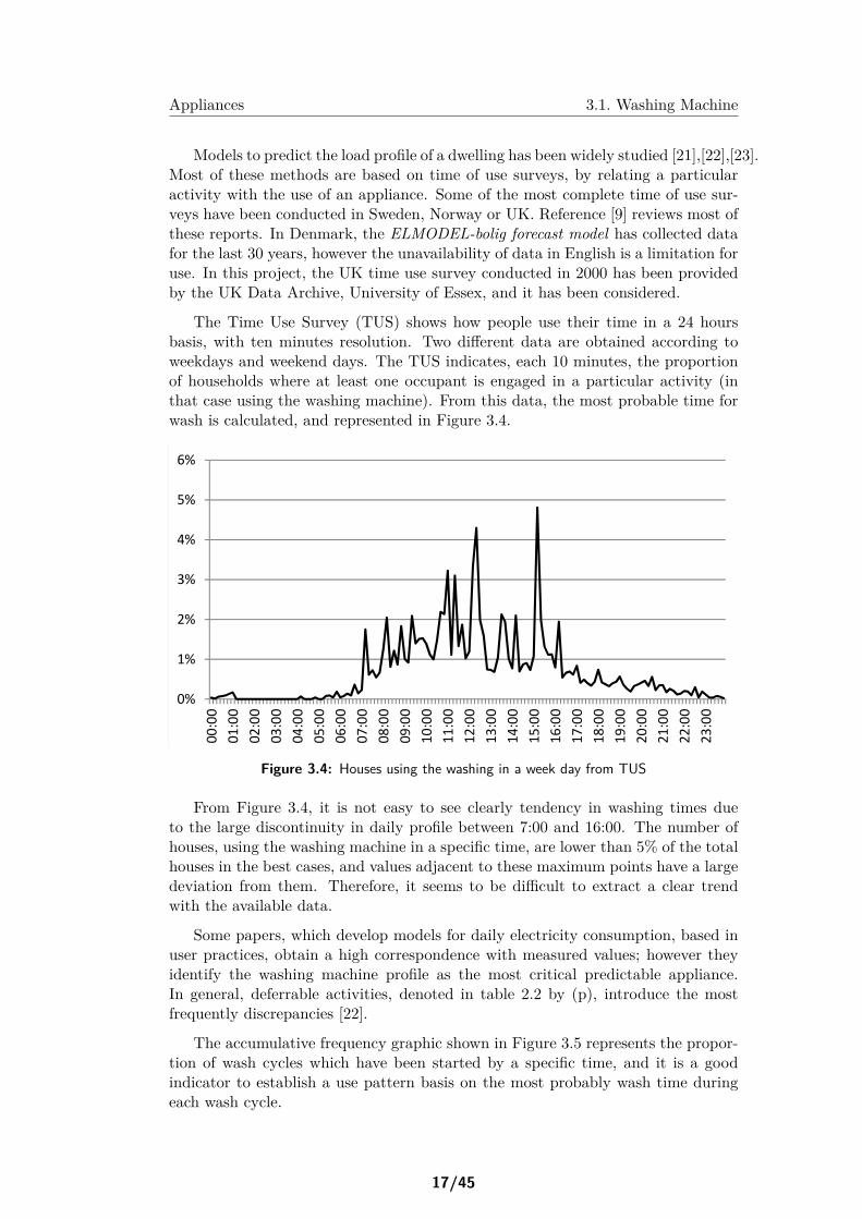
The Time Use Survey (TUS) shows how people use their time in a 24 hoursbasis, with ten minutes resolution. Two different data are obtained according toweekdays and weekend days. The TUS indicates, each 10 minutes, the proportionof households where at least one occupant is engaged in a particular activity (inthat case using the washing machine). From this data, the most probable time forwash is calculated, and represented in Figure 3.4.
0%
1%
2%
3%
4%
5%
6%
00:00
01:00
02:00
03:00
04:00
05:00
06:00
07:00
08:00
09:00
10:00
11:00
12:00
13:00
14:00
15:00
16:00
17:00
18:00
19:00
20:00
21:00
22:00
23:00
Figure 3.4: Houses using the washing in a week day from TUS
From Figure 3.4, it is not easy to see clearly tendency in washing times dueto the large discontinuity in daily profile between 7:00 and 16:00. The number ofhouses, using the washing machine in a specific time, are lower than 5% of the totalhouses in the best cases, and values adjacent to these maximum points have a largedeviation from them. Therefore, it seems to be difficult to extract a clear trendwith the available data.
Some papers, which develop models for daily electricity consumption, based inuser practices, obtain a high correspondence with measured values; however theyidentify the washing machine profile as the most critical predictable appliance.In general, deferrable activities, denoted in table 2.2 by (p), introduce the mostfrequently discrepancies [22].
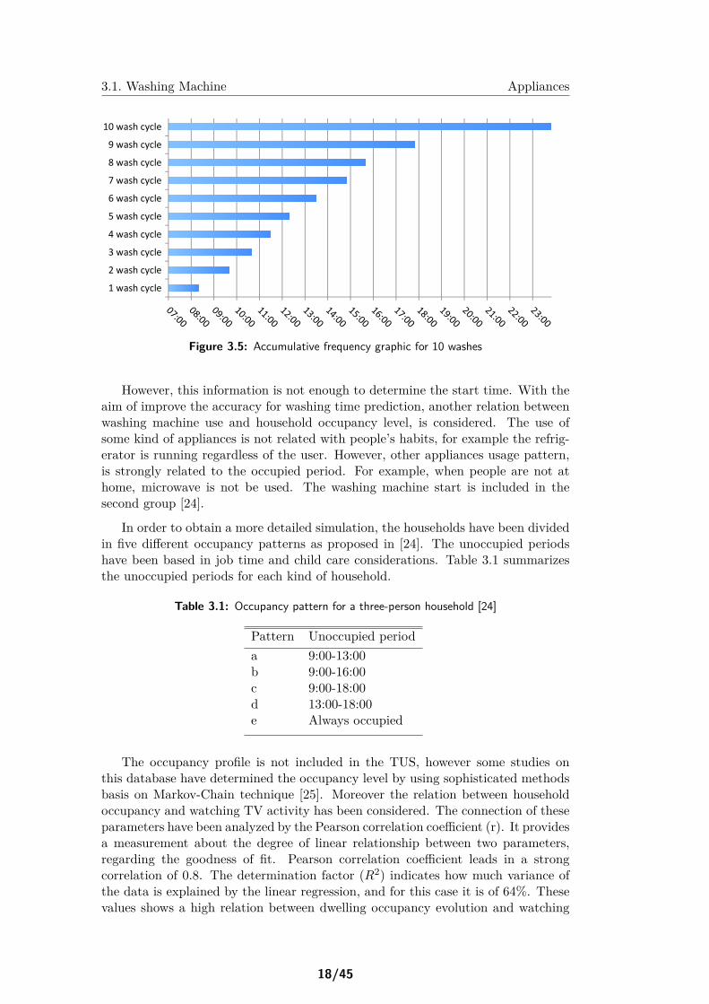
The accumulative frequency graphic shown in Figure 3.5 represents the propor-tion of wash cycles which have been started by a specific time, and it is a goodindicator to establish a use pattern basis on the most probably wash time duringeach wash cycle.
17/45
3.1. Washing Machine Appliances
1 wash cycle
2 wash cycle
3 wash cycle
4 wash cycle
5 wash cycle
6 wash cycle
7 wash cycle
8 wash cycle
9 wash cycle
10 wash cycle
Figure 3.5: Accumulative frequency graphic for 10 washes
However, this information is not enough to determine the start time. With theaim of improve the accuracy for washing time prediction, another relation betweenwashing machine use and household occupancy level, is considered. The use ofsome kind of appliances is not related with people’s habits, for example the refrig-erator is running regardless of the user. However, other appliances usage pattern,is strongly related to the occupied period. For example, when people are not athome, microwave is not be used. The washing machine start is included in thesecond group [24].
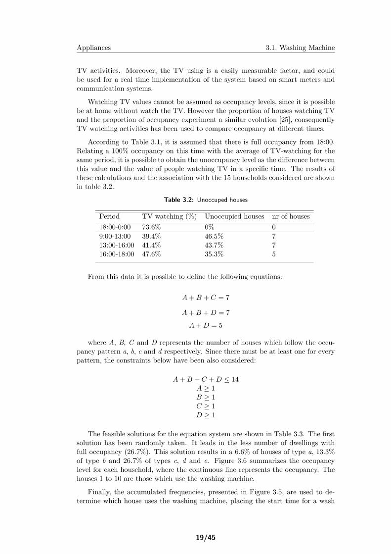
In order to obtain a more detailed simulation, the households have been dividedin five different occupancy patterns as proposed in [24]. The unoccupied periodshave been based in job time and child care considerations. Table 3.1 summarizesthe unoccupied periods for each kind of household.
Table 3.1: Occupancy pattern for a three-person household [24]
Pattern Unoccupied perioda 9:00-13:00b 9:00-16:00c 9:00-18:00d 13:00-18:00e Always occupied
The occupancy profile is not included in the TUS, however some studies onthis database have determined the occupancy level by using sophisticated methodsbasis on Markov-Chain technique [25]. Moreover the relation between householdoccupancy and watching TV activity has been considered. The connection of theseparameters have been analyzed by the Pearson correlation coefficient (r). It providesa measurement about the degree of linear relationship between two parameters,regarding the goodness of fit. Pearson correlation coefficient leads in a strongcorrelation of 0.8. The determination factor (R2) indicates how much variance ofthe data is explained by the linear regression, and for this case it is of 64%. Thesevalues shows a high relation between dwelling occupancy evolution and watching
18/45
Appliances 3.1. Washing Machine
TV activities. Moreover, the TV using is a easily measurable factor, and couldbe used for a real time implementation of the system based on smart meters andcommunication systems.
Watching TV values cannot be assumed as occupancy levels, since it is possiblebe at home without watch the TV. However the proportion of houses watching TVand the proportion of occupancy experiment a similar evolution [25], consequentlyTV watching activities has been used to compare occupancy at different times.
According to Table 3.1, it is assumed that there is full occupancy from 18:00.Relating a 100% occupancy on this time with the average of TV-watching for thesame period, it is possible to obtain the unoccupancy level as the difference betweenthis value and the value of people watching TV in a specific time. The results ofthese calculations and the association with the 15 households considered are shownin table 3.2.
Table 3.2: Unoccuped houses
Period TV watching (%) Unoccupied houses nr of houses18:00-0:00 73.6% 0% 09:00-13:00 39.4% 46.5% 713:00-16:00 41.4% 43.7% 716:00-18:00 47.6% 35.3% 5
From this data it is possible to define the following equations:
A+B + C = 7
A+B +D = 7A+D = 5
where A, B, C and D represents the number of houses which follow the occu-pancy pattern a, b, c and d respectively. Since there must be at least one for everypattern, the constraints below have been also considered:
A+B + C +D ≤ 14A ≥ 1B ≥ 1C ≥ 1D ≥ 1
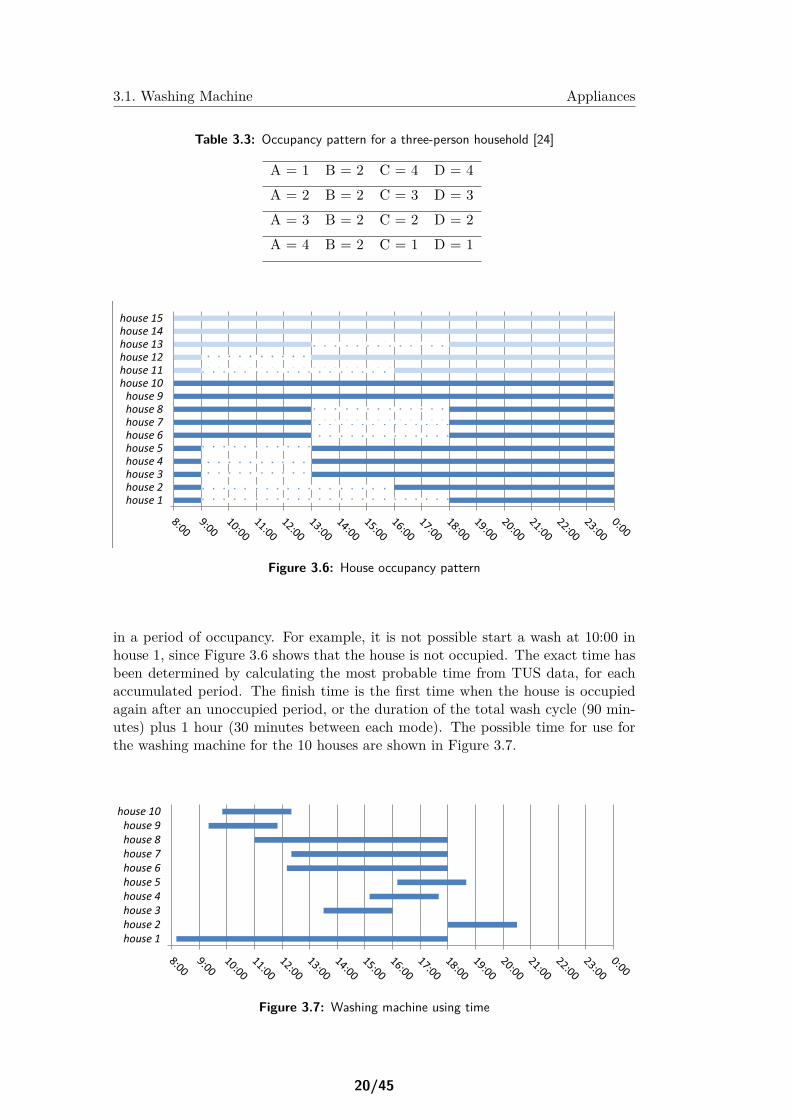
The feasible solutions for the equation system are shown in Table 3.3. The firstsolution has been randomly taken. It leads in the less number of dwellings withfull occupancy (26.7%). This solution results in a 6.6% of houses of type a, 13.3%of type b and 26.7% of types c, d and e. Figure 3.6 summarizes the occupancylevel for each household, where the continuous line represents the occupancy. Thehouses 1 to 10 are those which use the washing machine.
Finally, the accumulated frequencies, presented in Figure 3.5, are used to de-termine which house uses the washing machine, placing the start time for a wash
19/45
3.1. Washing Machine Appliances
Table 3.3: Occupancy pattern for a three-person household [24]
A = 1 B = 2 C = 4 D = 4A = 2 B = 2 C = 3 D = 3A = 3 B = 2 C = 2 D = 2A = 4 B = 2 C = 1 D = 1
house 1house 2house 3house 4house 5house 6house 7house 8house 9
house 10house 11house 12house 13house 14house 15
Figure 3.6: House occupancy pattern
in a period of occupancy. For example, it is not possible start a wash at 10:00 inhouse 1, since Figure 3.6 shows that the house is not occupied. The exact time hasbeen determined by calculating the most probable time from TUS data, for eachaccumulated period. The finish time is the first time when the house is occupiedagain after an unoccupied period, or the duration of the total wash cycle (90 min-utes) plus 1 hour (30 minutes between each mode). The possible time for use forthe washing machine for the 10 houses are shown in Figure 3.7.
house 1house 2house 3house 4house 5house 6house 7house 8house 9
house 10
Figure 3.7: Washing machine using time
20/45
3.2. Refrigerator
3.2 Refrigerator
Refrigerators and freezers represent the second largest energy consumption in ahousehold (Table 2.2). In this category, chest freezers, fridge freezers, uprightfreezers and refrigerators are included. The most common freezer appliance isthe fridge with refrigerator and chest freezer [20], however for this project a simplerefrigerator has been considered due to simplicity reasons. Moreover, the simulationof a fridge freezer is based on the same principles than a refrigerator, but consideringtwo cooling devices: refrigerator and chest freezer. Another limitation for the modelis the temperature variation due to number of door openings. Variations in foodstored is neither considered.
In recent years, the improvement in refrigerators design has made possible aconsumption of 156 kWh/year [16]. However most of the refrigerators reviewedconsume between 200 and 300 kWh/year with a rated power around 90 and 150W. This amount of peak power is not very significant, however the possibility ofcoordinating various refrigerators of different households, becomes interesting inorder to adapt consumption in real time [4]. The use of a thermal storage deviceto DSM has been already studied in the literature [29] [30], based on this ideathe thermal characteristics of a refrigerator are studied, and related with its loadprofile.
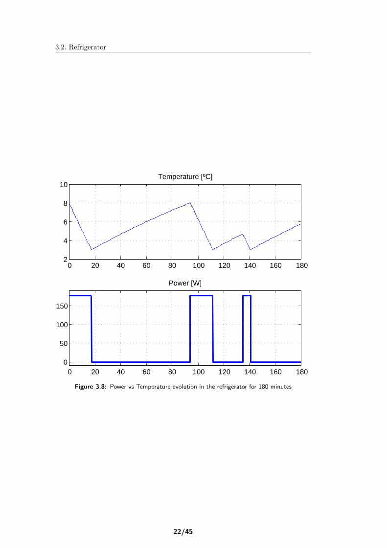
The function of a refrigerator is to preserve the aliments in a correct temper-ature, which usually is between 3 and 8◦C [31]. The operation to maintain thetemperature in the desired range is shown in Figure 3.8, and it consists of basi-cally in running the compressor when the superior temperature is reached; stop thecooling at inferior limit, and keep off the cooling until the temperature increasesagain.
The DSM is done by changing the temperature limits (which always should beincluded in the original limits, set between 3 and 8◦C) according to the necessitiesof the system. That is, when an optimal point (according to economic and energeticconsiderations) is reach, it is possible turn off the refrigerator, decreasing the totalcost and power losses in moments with high prices, and high power request. In thecase of a reduction in energy price or consumption decrement the refrigerator isturned on.
A very important factor in the energy consumption is the temperature of theroom where the refrigerator is placed and the number of times of door opening [32].For this project the room temperature is assumed as constant in 21◦C, since thefreezer is usually placed at kitchens, and it is the standard temperature for a house[31]. As mentioned, the effect of door opening is not taken into account.
The temperature evolution related with electrical power required has been de-scribed by [33] and is characterized by equation 3.1.
T (t+ 1) = ε · T(t) + (1 − ε)(Tamb(t) − η · P (t)A
) (3.1)
The parameters are described in table 3.4. In [30] the differential equationsfrom 3.1 are presented in order to obtain the temperature evolution for warming or
21/45
3.2. Refrigerator
0 20 40 60 80 100 120 140 160 1802
4
6
8
10Temperature [ºC]
0 20 40 60 80 100 120 140 160 1800
50
100
150
Power [W]
Figure 3.8: Power vs Temperature evolution in the refrigerator for 180 minutes
22/45
3.2. Refrigerator
cooling. This equations determines when the compressor is switched on 3.2 or off3.3.
T1(t) = T1(t1) − TON (t1)e− A
mct1
e− Amc
t + TON (t) (3.2)
where TON (t) = Tamb(t) − η·P (t)A
T2(t) = T2(t1) − Tamb(t1)e− A
mct1
e− Amc
t + Tamb(t) (3.3)
where,
Table 3.4: Refrigerator parameters
ε factor of inertia -η coefficient of performance 3A thermal insulation 6 W/◦Cmc thermal mass 1500 J/◦CTamb ambient temperature 22 ◦C
From equations the system has been simulated in Matlab. The scrpit, allowsthe introduction of a switching schedule, in order to obtain the power profile. Thenumerical values used for the simulation are included in table 3.4. This values, usedin [29], represent a good approximation to the refrigerator dynamics. Figure 3.8presents a 3 hours simulation from the Matlab model. As can be seen a completecycle takes 95 minutes. The considered refrigerator has a nominal power consump-tion of 177 W during 18 minutes. For simplification reasons the complete cycle willbe considered as 100 minutes and the working time per cycle of 20 minutes. Thisassumption leads in an energy demand of 59 Wh for a complete cycle.
The model runs autonomously, keeping the temperature in the limits, and pro-vides the power profile as shown in Figure 3.8. However, it is able to respond to anexternal order. If an increment in consumption is required, the refrigerator poweroutput will increase if the temperature is decreasing, and similar process is followedfor a consumption decrement. However, if an increment is required and the com-pressor is already running, or the temperature is in the lower limit, no modificationwill occur. This phenomenon occurs in the minute 135 of the Figure 3.8, when anincrement in consumption is required. After the temperature hits the lower limit,the compressor switches off and the temperature increases until 8◦C.
Although the refrigerator is a continuous run appliance, some modifications canbe done in its load profile in order to obtain a better performance. As mentionedbefore, the variations are based in an external signal which activates or deactivatesthe compressor. This idea is based on direct load control (DLC). By this manage-ment, it is possible to introduce the optimal control schedule for the refrigerator.
For this project, two different scenarios has been considered to manage therefrigerator. The first one refers to a normal operation, where the temperature
23/45
3.2. Refrigerator
never exceeds 8◦C. However, it is possible to move the cooling periods within thetime range in order to obtain a better performance in price or energy losses. Forexample it is possible bring forward a cooling period, as shown in Figure 3.8 inminute 135, if there is a lower price at that time.
The extension of the temperature range, results in a larger cycle duration. Thismanagement makes possible to maintain the refrigerator in on or off during con-tinue periods of more than 20 or 80 minutes respectively. It is because, decreasefrom a temperature greater than 8◦to 3◦needs more energy, and consequently alarger on period. In contrast it is possible maintain the refrigerator in off duringmore time starting from 3◦C, until a temperature greater than 8◦C. The benefit oflonger periods in on or off is to take advantage of time intervals, where runningthe refrigerator entails a lower price or energy losses, and on the contrary avoidunfavorable periods.
Due to simplicity reasons, in order to match up the time intervals from powerconsumption with the washing machine use pattern, the activation periods are of 10minutes durations. A increment of temperature from 8◦C, during an extra periodof 10 minutes, results in a maximum temperature of 10.5◦C. This second scenarioconsiders a cycle duration of 150 minutes and 30 running minutes. The optimalcontrol will be obtained for both cases and compared with the original management.
24/45
Chapter 4
Optimization
In order to achieve the minimum losses in distribution lines, and electricity costfor final user, an optimization of the washing machine and refrigerator use hasbeen conducted. This chapter provides a detailed explanation of how the grid ismodeled in Matlab. Chapter 3 focused on the behavior of the washing machineand refrigerator from the point of view of technical operation and time of use.These characteristics and limitations are used here to model the electrical systemaccording to operation requirements.
4.1 Problem Formulation
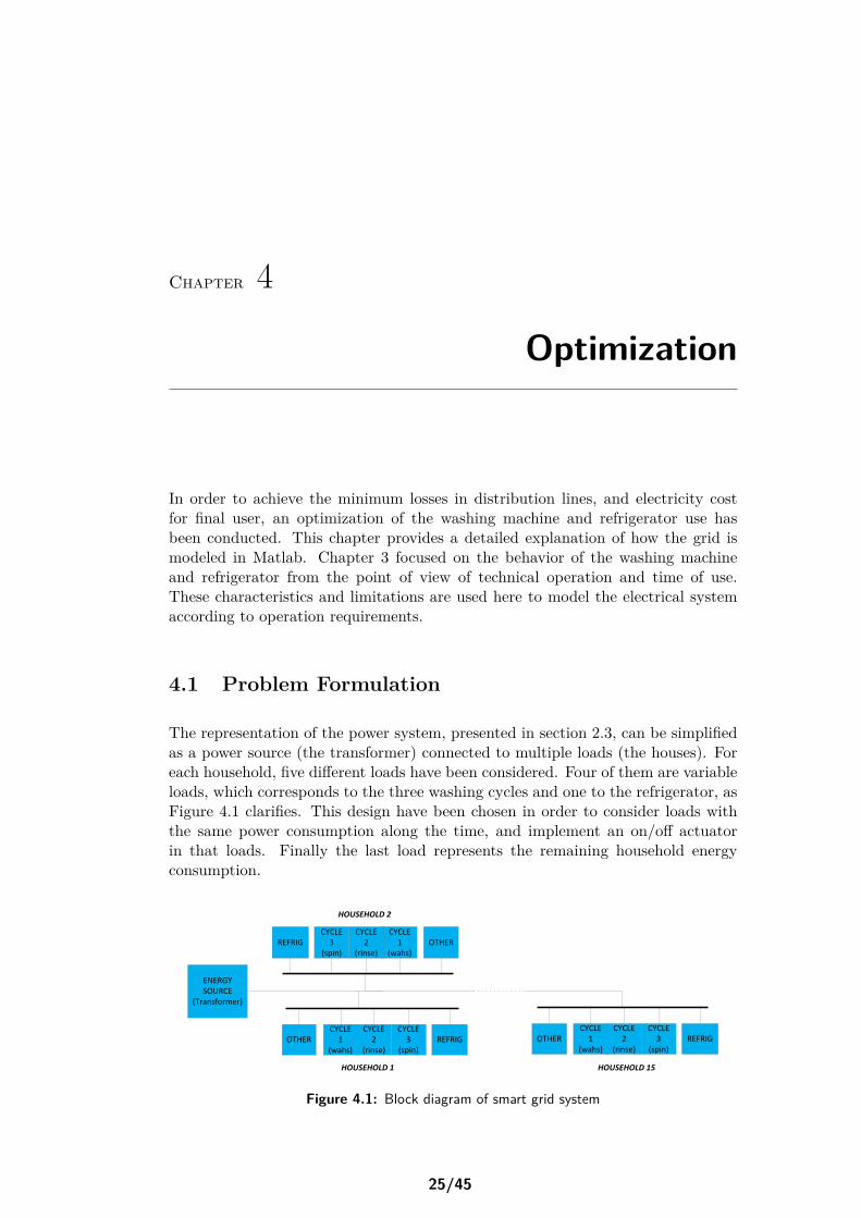
The representation of the power system, presented in section 2.3, can be simplifiedas a power source (the transformer) connected to multiple loads (the houses). Foreach household, five different loads have been considered. Four of them are variableloads, which corresponds to the three washing cycles and one to the refrigerator, asFigure 4.1 clarifies. This design have been chosen in order to consider loads withthe same power consumption along the time, and implement an on/off actuatorin that loads. Finally the last load represents the remaining household energyconsumption.
ENERGY SOURCE
(Transformer)
CYCLE 1
(wahs)
CYCLE 2
(rinse)
CYCLE 3
(spin)REFRIG OTHER
CYCLE 1
(wahs)
CYCLE 2
(rinse)
CYCLE 3
(spin)REFRIGOTHER
HOUSEHOLD 2
HOUSEHOLD 1
CYCLE 1
(wahs)
CYCLE 2
(rinse)
CYCLE 3
(spin)REFRIGOTHER
HOUSEHOLD 15
Figure 4.1: Block diagram of smart grid system
25/45
4.1. Problem Formulation Optimization
The washing machine pattern limits the time of use from around 8:00 to 0:00Figure 3.7, in order to simplify the optimization system and reduce the calculationtime this has been considered as the optimization period. The analysis resolution(time steps) is determined by the smallest operation time of the appliances, in thiscase it is 10 minutes, which corresponds to the last washing cycle (spin). A smallerresolution will result in a better control of the temperature in the refrigerator,since increments of 1◦C or even 0.5◦C could be considered. However it implies anincrease in the number of studied steps, which results in a much higher run time ofthe optimization algorithm.
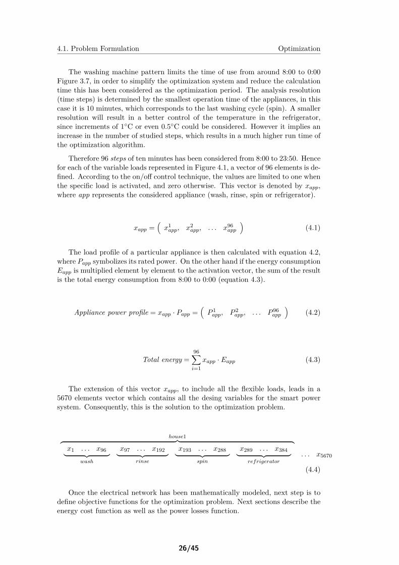
Therefore 96 steps of ten minutes has been considered from 8:00 to 23:50. Hencefor each of the variable loads represented in Figure 4.1, a vector of 96 elements is de-fined. According to the on/off control technique, the values are limited to one whenthe specific load is activated, and zero otherwise. This vector is denoted by xapp,where app represents the considered appliance (wash, rinse, spin or refrigerator).
xapp =(x1app, x2
app, . . . x96app
)(4.1)
The load profile of a particular appliance is then calculated with equation 4.2,where Papp symbolizes its rated power. On the other hand if the energy consumptionEapp is multiplied element by element to the activation vector, the sum of the resultis the total energy consumption from 8:00 to 0:00 (equation 4.3).
Appliance power profile = xapp · Papp =(P 1app, P 2
app, . . . P 96app
)(4.2)
Total energy =96∑i=1
xapp · Eapp (4.3)
The extension of this vector xapp, to include all the flexible loads, leads in a5670 elements vector which contains all the desing variables for the smart powersystem. Consequently, this is the solution to the optimization problem.
house1︷ ︸︸ ︷x1 . . . x96︸ ︷︷ ︸
wash
x97 . . . x192︸ ︷︷ ︸rinse
x193 . . . x288︸ ︷︷ ︸spin
x289 . . . x384︸ ︷︷ ︸refrigerator
. . . x5670
(4.4)
Once the electrical network has been mathematically modeled, next step is todefine objective functions for the optimization problem. Next sections describe theenergy cost function as well as the power losses function.
26/45
4.2. Energy cost function
4.2 Energy cost function
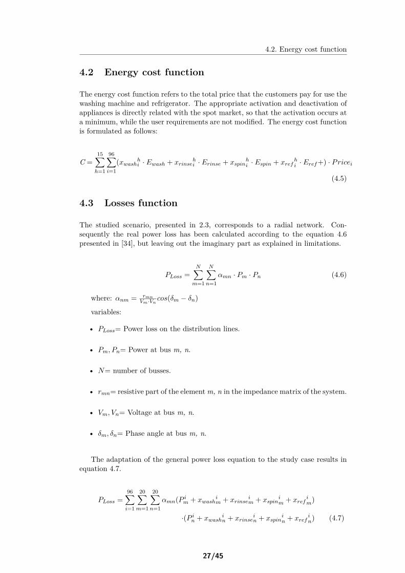
The energy cost function refers to the total price that the customers pay for use thewashing machine and refrigerator. The appropriate activation and deactivation ofappliances is directly related with the spot market, so that the activation occurs ata minimum, while the user requirements are not modified. The energy cost functionis formulated as follows:
C =15∑h=1
96∑i=1
(xwashhi · Ewash + xrinsehi · Erinse + xspin
hi · Espin + xref
hi · Eref+) · Pricei
(4.5)
4.3 Losses function
The studied scenario, presented in 2.3, corresponds to a radial network. Con-sequently the real power loss has been calculated according to the equation 4.6presented in [34], but leaving out the imaginary part as explained in limitations.
PLoss =N∑m=1
N∑n=1
αmn · Pm · Pn (4.6)
where: αnm = rmnVm·Vn
cos(δm − δn)
variables:
• PLoss= Power loss on the distribution lines.
• Pm, Pn= Power at bus m, n.
• N= number of busses.
• rmn= resistive part of the elementm, n in the impedance matrix of the system.
• Vm, Vn= Voltage at bus m, n.
• δm, δn= Phase angle at bus m, n.
The adaptation of the general power loss equation to the study case results inequation 4.7.
PLoss =96∑i=1
20∑m=1
20∑n=1
αmn(P im + xwashim + xrinse
im + xspin
im + xref
im)
·(P in + xwashin + xrinse
in + xspin
in + xref
in) (4.7)
27/45
4.4. Optimization using Matlab Optimization Toolbox
Although the voltage and phase angle change with power variations, it remainsalmost constant because it may not vary much, and consequently α has been con-sidered as constant. The values of V and δ have been obtained from a load flowconducted in the DIgSILENT model, which is presented in Chapter 5.
The result of equation 4.7 does not represent any final result for minimization,since it is the sum of power loss for each period. However, it represnets the totalpower loss, and it is an effective value to account for the minimization of total energylosses. The real value of energy loss will be calculated by using the DIgSILENTmodel.
4.4 Optimization using Matlab Optimization Toolbox
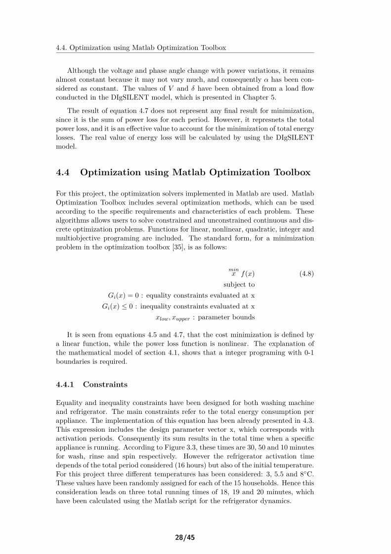
For this project, the optimization solvers implemented in Matlab are used. MatlabOptimization Toolbox includes several optimization methods, which can be usedaccording to the specific requirements and characteristics of each problem. Thesealgorithms allows users to solve constrained and unconstrained continuous and dis-crete optimization problems. Functions for linear, nonlinear, quadratic, integer andmultiobjective programing are included. The standard form, for a minimizationproblem in the optimization toolbox [35], is as follows:
minx f(x) (4.8)
subject toGi(x) = 0 : equality constraints evaluated at x
Gi(x) ≤ 0 : inequality constraints evaluated at xxlow, xupper : parameter bounds
It is seen from equations 4.5 and 4.7, that the cost minimization is defined bya linear function, while the power loss function is nonlinear. The explanation ofthe mathematical model of section 4.1, shows that a integer programing with 0-1boundaries is required.
4.4.1 Constraints
Equality and inequality constraints have been designed for both washing machineand refrigerator. The main constraints refer to the total energy consumption perappliance. The implementation of this equation has been already presented in 4.3.This expression includes the design parameter vector x, which corresponds withactivation periods. Consequently its sum results in the total time when a specificappliance is running. According to Figure 3.3, these times are 30, 50 and 10 minutesfor wash, rinse and spin respectively. However the refrigerator activation timedepends of the total period considered (16 hours) but also of the initial temperature.For this project three different temperatures has been considered: 3, 5.5 and 8◦C.These values have been randomly assigned for each of the 15 households. Hence thisconsideration leads on three total running times of 18, 19 and 20 minutes, whichhave been calculated using the Matlab script for the refrigerator dynamics.
28/45
4.4. Optimization using Matlab Optimization Toolbox
Besides the general energy constraints, other particular limitations have to beconsidered for each kind of appliance. For the washing machine, it can have onlyone cycle at a time and maintain the correct order of operation (wash, rinse andspin). In addition, the cycles cannot be broken.
Finally, the constraints necessary for the refrigerator have been designed de-pending on the initial temperature, and the maximum temperature which could bereach for each individual refrigerator. The upper bound temperature can be chosenfrom the scenarios described in section 3.2, a normal operation on 8◦C (scenario 1)or 10.5◦C (scenario 2). While the initial temperature has been randomly assignedto each refrigerator, the temperature range leads in two different kind of inequalityconstraints.
The bounds have been set according to the use pattern calculation (Figure 3.7)for the washing machine, while for the refrigerator the whole period is considered asfeasible, and the limitations are introduced exclusively by the constraints equations.
4.4.2 Solver Functions
As conclusion the minimization problem includes the following requirements:
• Integer boundaries solution set (binary).
• Linear Cost function.
• Nonlinear Loss function.
• Inequality linear constraints.
• Equality linear constraints.
However any of the solvers present in Matlab Optimization Toolbox fulfills allthe requirements. In order to achieve a proper optimization, the minimizationproblem has been divided in two subproblems. First refers to the cost optimization,which has been processed by using the bintprog solver. This algorithm is based indual-simplex and branch&bound methods. Dual-simplex is a common method tosolve linear functions, widely explained for example in [27]. Branch&bound methodis an iterative optimization algorithm which finds the best integer solution for agiven problem, based in a tree structure of feasible solutions [36]. The bounds are0-1 non selectable.
On the other hand, the loss power function has been solved using the optimizerfmincon. Fmincon solves nonlinear functions, with linear and nonlinear constraints,within a selectable range of bounds. This solver uses gradient based search methods.That means that the minimum is obtained by computing the values pointed by thegradient of the objective function, until a minimum is found. This method is basedon the knowledge that the gradient vector points in the direction of maximun
29/45
4.4. Optimization using Matlab Optimization Toolbox
increase of a function [37]. Hence one of the task of the optimizer is to calculatethe search direction. Some methods can be chosen in fmincon solver, in this projectthe interior point method has been used due to a smaller run time in contrast withother methods with a better accuracy but much longer run time.
Gradient search methods need an initial point from where the gradient is cal-culated. The initial point for fmincon is the optimal for a minimum energy cost(result of the cost optimization with bintprog). However the result is not an integersolution.
The noninterger result is actually a weighted solution of the optimal integerpoint. It means that each single objective value has a significant value for theminimum result, and the greater numbers represent the most beneficial activationintervals. The proposed methodology carries several optimizations using fmincon,and after each optimization the solution and the boundaries are improved.
It is done by fixing to 1 (activate) the biggest value of the solution, and adaptthe boundaries according to the characteristics of this point. For example if itcorresponds to a spin cycle all the other points for this cycle are set to 0. Thisiterative optimization procedure is repeated until an integer solution is obtained.
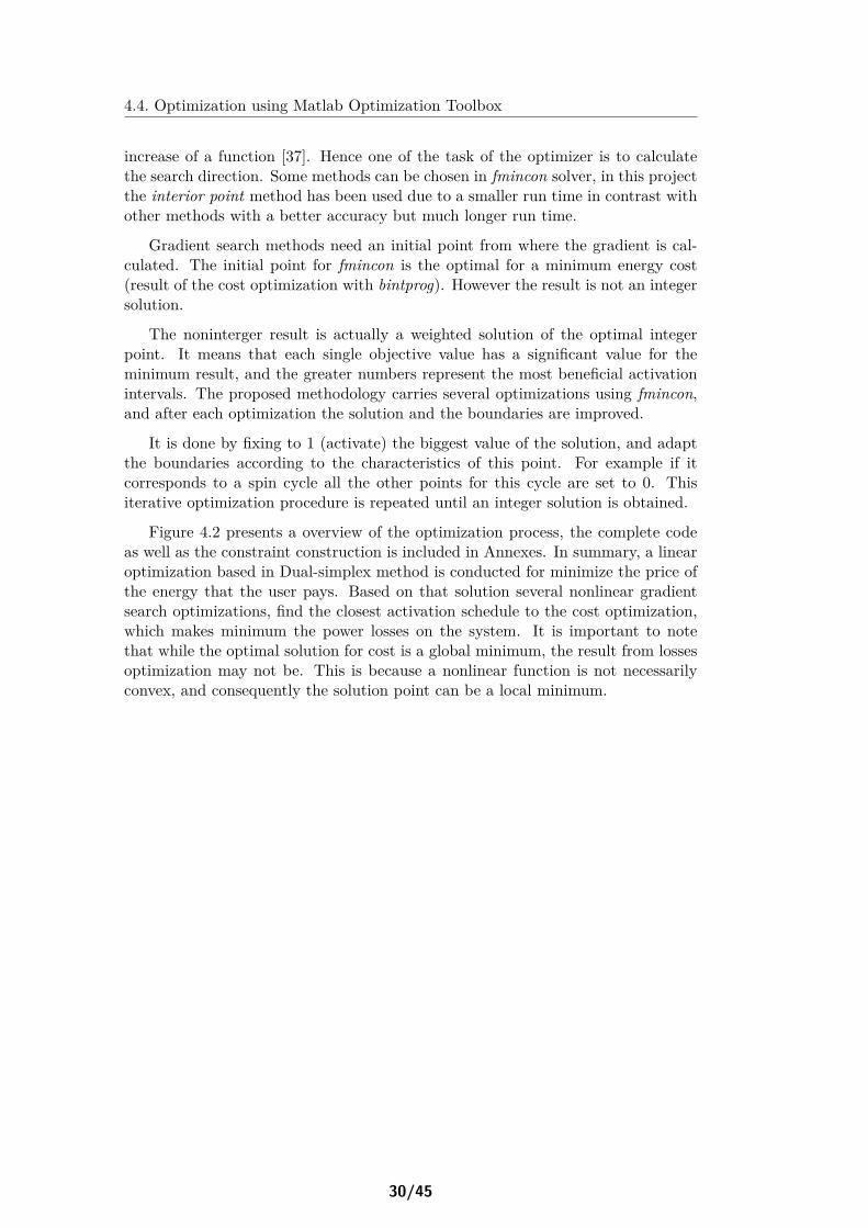
Figure 4.2 presents a overview of the optimization process, the complete codeas well as the constraint construction is included in Annexes. In summary, a linearoptimization based in Dual-simplex method is conducted for minimize the price ofthe energy that the user pays. Based on that solution several nonlinear gradientsearch optimizations, find the closest activation schedule to the cost optimization,which makes minimum the power losses on the system. It is important to notethat while the optimal solution for cost is a global minimum, the result from lossesoptimization may not be. This is because a nonlinear function is not necessarilyconvex, and consequently the solution point can be a local minimum.
30/45
4.5. Optimization results
LOAD WASHING LIMITS AND INITIAL
TEMPERATURE
COST OPTIMIZATION
(bintprog)
Construction of initial point
LOSS ENERGY OPTIMIZATON
(fmincon)
Adaptation of boundaries
Fix the maximun value
Optimization finished
COST COMPARATION
PRINT RESULTS
NO
YES
Boundaries & Constraints definition
IterativeOptimization
Figure 4.2: Flow Chart general algorithm
4.5 Optimization results
This section presents the results of the optimization process explained in Figure4.2. The specific study place has been described in 2.3, as well as the power profileand the transmission lines characteristics, which are necessaries to compute thepower losses in equation 4.7. The use pattern of the washing machine is deducedin Figure 3.7. The behavior of the refrigerator has led in two different scenarios ofmaximum temperature (8◦C and 10.5◦C) described in 3.2.
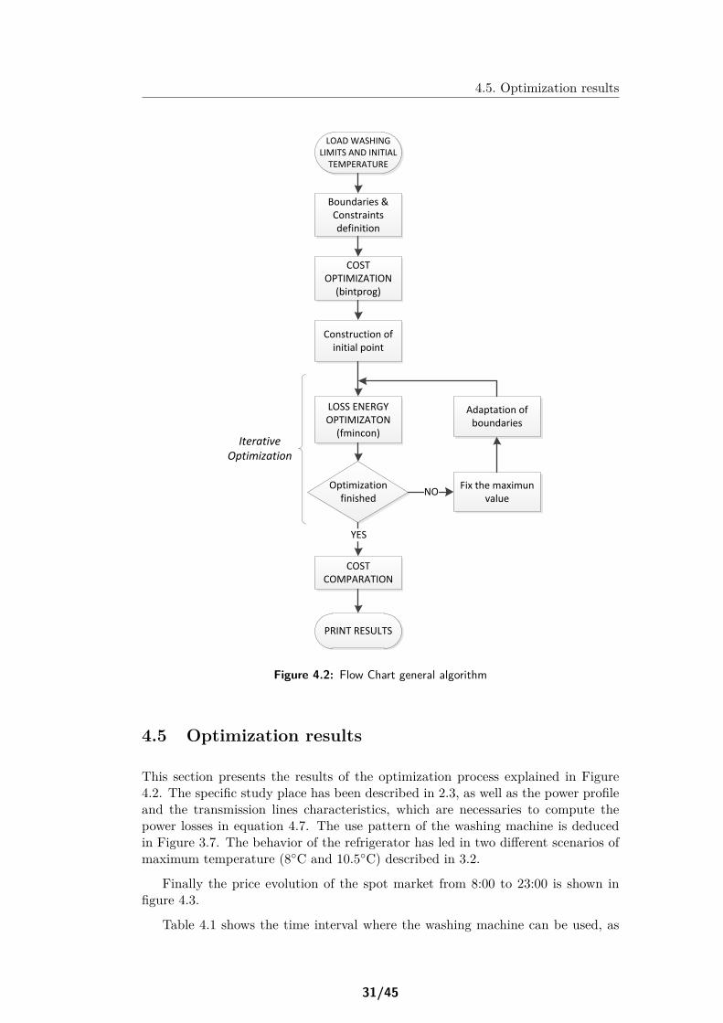
Finally the price evolution of the spot market from 8:00 to 23:00 is shown infigure 4.3.
Table 4.1 shows the time interval where the washing machine can be used, as
31/45
4.5. Optimization results
0,2
0,3
0,4
0,5
0,6
0,7
Energy Price [DKK/kWh]
Figure 4.3: Spot Market price for electricity
well as the total duration of this interval. The initial temperature for each house isalso included. Finally, the optimal schedule times for each washing cycle is shown.The results are for the Scenario 1, however the schedule for Scenario 2 is similar,except in four houses, where the variations are less than 30 minutes, and it is notshown.
INPUTS OUTPUTSHouse Start Finish Duration Initial Wash Rinse Spin
temperature1 9:20 11:50 2:30 3 10:00 10:40 11:302 - - - 5.5 - - -3 11:00 18:00 7:00 8 15:20 16:10 17:004 12:10 18:00 5:50 3 15:10 15:40 17:005 15:10 17:40 2:30 5.5 15:10 15:40 16:306 8:10 18:00 9:50 8 15:10 15:40 16:407 - - - 3 - - -8 13:30 16:00 2:30 5.5 14:10 14:40 15:409 - - - 8 - - -10 9:20 11:50 2:30 3 15:10 15:40 16:3011 - - - 5.5 - - -12 9:50 12:20 2:30 8 10:40 11:10 12:0013 16:10 18:40 2:30 3 16:10 16:40 17:3014 - - - 5.5 - - -15 18:00 20:30 2:30 8 18:00 19:10 20:10
Table 4.1: Optimization inputs and washing time results (Scenario 1)
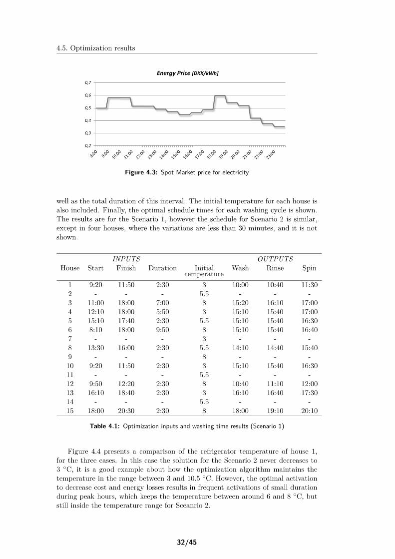
Figure 4.4 presents a comparison of the refrigerator temperature of house 1,for the three cases. In this case the solution for the Scenario 2 never decreases to3 ◦C, it is a good example about how the optimization algorithm maintains thetemperature in the range between 3 and 10.5 ◦C. However, the optimal activationto decrease cost and energy losses results in frequent activations of small durationduring peak hours, which keeps the temperature between around 6 and 8 ◦C, butstill inside the temperature range for Sceanrio 2.
32/45
4.5. Optimization results
0
2
4
6
8
10
12
8:00 9:00 10:00 11:00 12:00 13:00 14:00 15:00 16:00 17:00 18:00 19:00 20:00 21:00 22:00 23:00
Tem
per
atu
re [
⁰C]
Time [Hour]
Original
Scenario 1
Scenario 2
Figure 4.4: Temperature in refrigerator of house 1 for the three scenarios
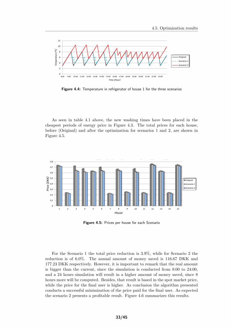
As seen in table 4.1 above, the new washing times have been placed in thecheapest periods of energy price in Figure 4.3. The total prices for each house,before (Original) and after the optimization for scenarios 1 and 2, are shown inFigure 4.5.
0
0,1
0,2
0,3
0,4
0,5
0,6
0,7
1 2 3 4 5 6 7 8 9 10 11 12 13 14 15
Pri
ce [
DK
K]
House
Original
Scenario 1
Scenario 2
0
0,1
0,2
0,3
0,4
0,5
0,6
0,7
0,8
1 2 3 4 5 6 7 8 9 10 11 12 13 14 15
Pri
ce [
DK
K]
House
Original
Scenario 1
Scenario 2
Figure 4.5: Prices per house for each Scenario
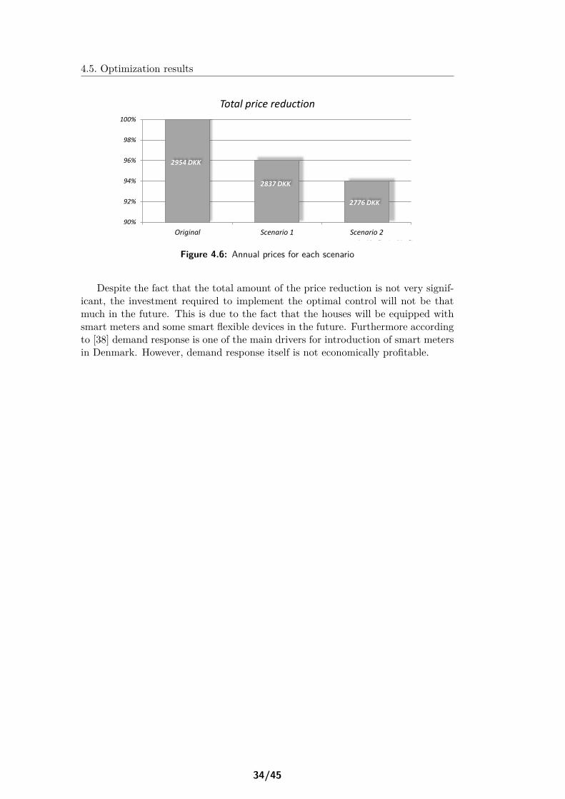
For the Scenario 1 the total price reduction is 3.9%, while for Scenario 2 thereduction is of 6.0%. The annual amount of money saved is 116.67 DKK and177.23 DKK respectively. However, it is important to remark that the real amountis bigger than the current, since the simulation is conducted from 8:00 to 24:00,and a 24 hours simulation will result in a higher amount of money saved, since 8hours more will be computed. Besides, that result is based in the spot market price,while the price for the final user is higher. As conclusion the algorithm presentedconducts a successful minimization of the price paid for the final user. As expectedthe scenario 2 presents a profitable result. Figure 4.6 summarizes this results.
33/45
4.5. Optimization results
0,2
0,3
0,4
0,5
0,6
0,7
0,8
Pri
ce [
DK
K]
90%
92%
94%
96%
98%
100%
Original Scenario 1 Scenario 2
Total price reduction
2954 DKK
2837 DKK
2776 DKK
Figure 4.6: Annual prices for each scenario
Despite the fact that the total amount of the price reduction is not very signif-icant, the investment required to implement the optimal control will not be thatmuch in the future. This is due to the fact that the houses will be equipped withsmart meters and some smart flexible devices in the future. Furthermore accordingto [38] demand response is one of the main drivers for introduction of smart metersin Denmark. However, demand response itself is not economically profitable.
34/45
Chapter 5
Modeling
This chapter provides a description of the topology and modeling of the networkin DIgSILENT Power Factory. The model is used to obtain the necessary datato implement the power loss function as well as to compare the results after theoptimal management with the original case.
5.1 System description
The test system is based on Section 2.3. The external grid supplies the energynecessary for the households. The control is based in a DLC (direct load control)model of flexible loads. Hence two different load elements represent each household.A fix load represents the normal power profile, while a variable load implementsthe optimal consumption of washing machine and refrigerator. Figure 5.1 showsthe DIgSILENT implementation.
The values included in the model are the result from a power flow simulation,conducted with average power consumption values, in order to obtain V and δ foreach bus (section 4.3).
5.2 Implementation of optimal results
The optimal control calculated in Chapter 4 has been implemented in the model.Figure 5.2 presents a comparative of the total active power, supplied by the maingrid, for each scenario. The resultant curve for both scenarios, 1 and 2, showshow the optimal control of the appliances leads in a flatten curve than the original.Moreover, the peaks have been reduced or avoided.
35/45
5.2. Implementation of optimal results Modeling
PowerFactory 14.1.3
Project: Graphic: Grid Date: 5/22/2013 Annex:
Terminal 40,41920,9981-0,1181
T 120,41920,9981-0,1186
E 5
0,41920,9980-0,1196
T 10
0,41920,9981-0,1185
Terminal 30,41940,9985-0,1090
E 4
0,41930,9984-0,1099
E 10,41940,9985-0,1091
E 3
0,41930,9985-0,1092
E 2
0,41930,9984-0,1099
Terminal 2
0,41960,9990-0,0962
M 6
0,41960,9989-0,0968
M 40,41960,9990-0,0963
M 2
0,41950,9989-0,0978
M 1
0,41950,9989-0,0969
Terminal 10,41980,9995-0,0824
M 10
0,41980,9995-0,0830
M 8
0,41980,9995-0,0829
M 5
0,41980,9994-0,0840
Terminal 00,42001,0000-0,0696
GridTerminal 10.5 kV10,50001,00000,0000
M 3
0,41980,9994-0,0838
Line (4)0,00-0,001,21
-0,000,001,21
Line (3)
0,01-0,002,59
-0,010,002,59
House 13
0,00-0,00
Flex App 13
0,00-0,00
House 15
0,00-0,00
Line H15
0,00-0,000,47
-0,000,000,47
Flex App 1..
0,00-0,00
Line H13
0,00-0,000,47
-0,000,000,47
House 14
0,00-0,00
Line H14
0,00-0,000,30
-0,000,000,30
Flex App 14
0,00-0,00
Line H12
0,00-0,000,42
-0,000,000,42
House 12
0,00-0,00
Flex App 12
0,00-0,00
Flex App 9
0,00-0,00
Line H9
0,00-0,000,19
-0,000,000,19
House 9
0,00-0,00
Flex App 11
0,00-0,00
House 11
0,00-0,00
Line H11
0,00-0,000,16
-0,000,000,16
Line H10
0,00-0,000,64
-0,000,000,64
House 10
0,00-0,00
Flex App 10
0,00-0,00
Flex App 8
0,00-0,00
Line H7
0,00-0,000,19
-0,000,000,19
House 8
0,00-0,00
Line H8
0,00-0,000,62
-0,000,000,62
House 7
0,00-0,00
Flex App 7
0,00-0,00
Line H6
0,00-0,000,93
-0,000,000,93
House 6
0,00-0,00
Flex App 6
0,00-0,00
Flex App 5
0,00-0,00
House 5
0,00-0,00
Line H5
0,00-0,000,54
-0,000,000,54
Line H1
0,00-0,000,92
-0,000,000,92
Line H4
0,00-0,000,66
-0,000,000,66
Line (2)
0,01-0,004,83
-0,010,004,83
Flex App 4
0,00-0,00
House 4
0,00-0,00
Flex App 3
0,00-0,00
House 3
0,00-0,00
Line H3
0,00-0,000,69
-0,000,000,69
Flex App 2
0,00-0,00
House 2
0,00-0,00
Line H2
0,00-0,000,89
-0,000,000,89
Line (1)
0,02-0,007,92
-0,020,007,92
Flex App 1
0,00-0,00
House 1
0,00-0,00
Transformer
0,02-0,004,05
-0,020,004,05
External Grid0,02 MW-0,00 ..1,00
DIg
SILE
NT
Figure 5.1: Grid modeled in DigSilent
36/45
Modeling 5.2. Implementation of optimal results
0
10
20
30
40
50
60
8:00 9:00 10:00 11:00 12:00 13:00 14:00 15:00 16:00 17:00 18:00 19:00 20:00 21:00 22:00 23:00 0:00
Po
wer
[kW
]
Time [hours]
Scenario 2
Original
Scenario 1
Figure 5.2: Power profile of the system for each scenario
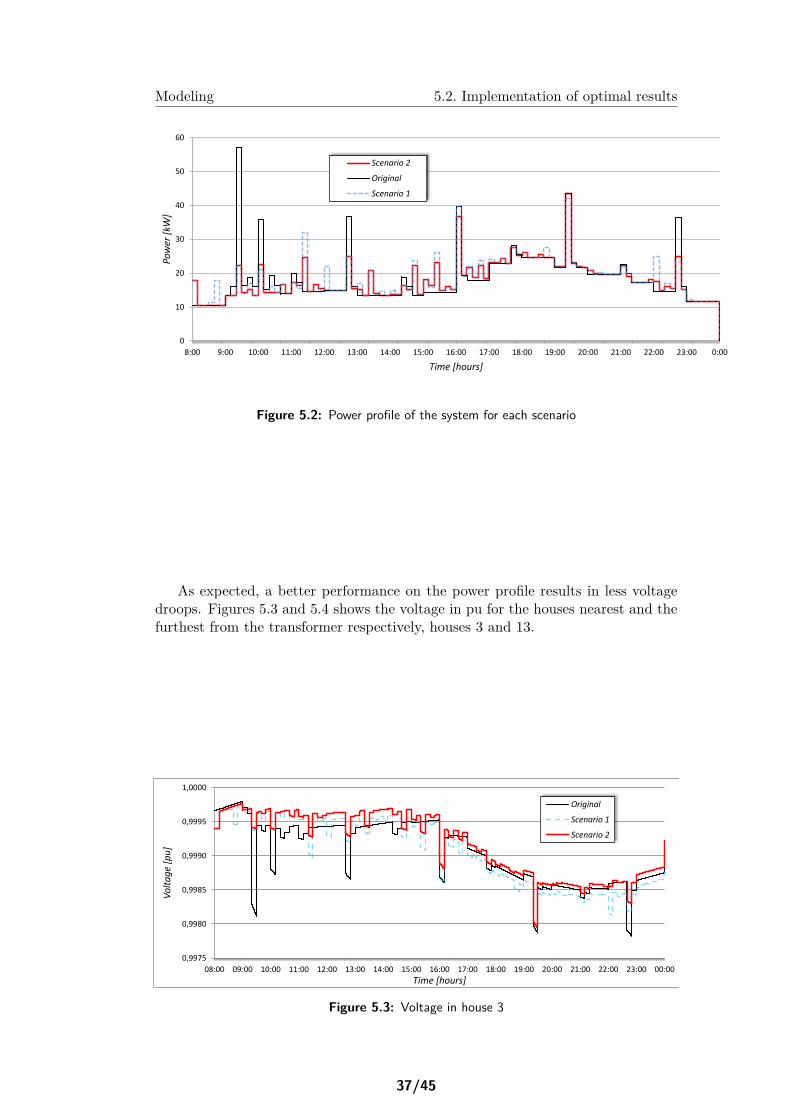
As expected, a better performance on the power profile results in less voltagedroops. Figures 5.3 and 5.4 shows the voltage in pu for the houses nearest and thefurthest from the transformer respectively, houses 3 and 13.
0,9975
0,9980
0,9985
0,9990
0,9995
1,0000
08:00 09:00 10:00 11:00 12:00 13:00 14:00 15:00 16:00 17:00 18:00 19:00 20:00 21:00 22:00 23:00 00:00
Vo
lta
ge
[pu
]
Time [hours]
Original
Scenario 1
Scenario 2
Figure 5.3: Voltage in house 3
37/45
5.3. Energy Losses
0,99
0,992
0,994
0,996
0,998
1
08:00 09:00 10:00 11:00 12:00 13:00 14:00 15:00 16:00 17:00 18:00 19:00 20:00 21:00 22:00 23:00 00:00
Vo
lta
ge
[pu
]
Time [hours]
Original
Scenario 1
Scenario 2
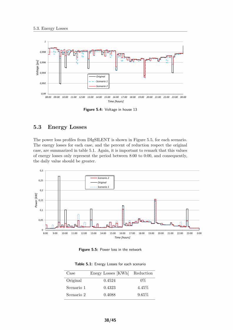
Figure 5.4: Voltage in house 13
5.3 Energy Losses
The power loss profiles from DIgSILENT is shown in Figure 5.5, for each scenario.The energy losses for each case, and the percent of reduction respect the originalcase, are summarized in table 5.1. Again, it is important to remark that this valuesof energy losses only represent the period between 8:00 to 0:00, and consequently,the daily value should be greater.
0
0,05
0,1
0,15
0,2
0,25
0,3
8:00 9:00 10:00 11:00 12:00 13:00 14:00 15:00 16:00 17:00 18:00 19:00 20:00 21:00 22:00 23:00 0:00
Po
wer
[kW
]
Time [hours]
Scenario 2
Original
Scenario 1
Figure 5.5: Power loss in the network
Table 5.1: Energy Losses for each scenario
Case Enegy Losses [KWh] ReductionOriginal 0.4524 0%Scenario 1 0.4323 4.45%Scenario 2 0.4088 9.65%
38/45

5.3. Energy Losses
The simulation results show that the method proposed is able to decrease theenergy losses for both scenarios.
39/45

5.3. Energy Losses
40/45
Chapter 6
Conclusion and future work
The objective of this project was to develop an intelligent management system forresidential loads. The project includes the study of residential loads, use pattern,optimization and modeling.
The distribution of residential electricity energy consumption in different loadshave been studied, and the most convenient appliances to implement a DSM havebeen presented. A way to convert washing machine and refrigerator in flexibleloads, has been developed. Two different methods have been proposed: so that theuser experience does not change and increasing the temperature of the refrigeratorduring some periods.
An optimization was conducted to find the best operation for the washing ma-chine and refrigerator. The operation results show the benefits of the DSM. Theprice that the user pays for the electrical energy and in the energy losses in the dis-tribution system have been properly reduced. The results of the simulations showthat the energy quality, measured by the voltage drop, experiment a significantimprovement.
As future work this report recommends, to investigate the control of otherappliances. A real time control for the refrigerator based on frequency variationscould be studied. Finally a longer simulation period will lead on a more accurateresult.
41/45

Bibliography
[1] G. Deconinck, B. Decroix, Smart Metering Tariff Schemes Combined withDistributed Energy Resources, K.U.Leuven, ESAT ELECTA Belgium
[2] Clark W. Gellins, The Concept of Demand-Side Management for Electric Util-ities, IEEE, 1985
[3] Bettina HIRL, Residential Energy Consumption and Efficiency Trends, Eu-ropean Commission, Joint Research Centre, Institute for Energy, EEDAL 11Conference, Copenhagen, Denmark, 2011
[4] David G. Infield, Joe Short, Chris Horne, Leon L. Freris, Potential for DomesticDynamic Demand-Side Management in the UK, IEEE 2007
[5] Demand-Side Management: Concepts and Methods, Clark W. Gellings, JohnH. Chamberlin, The Fairmont Press Inc.,Lilburn, GA, 1987
[6] Statistics Denmark - StatBank. ENE1N: Energy Accounts in physical units byindustry and type
[7] B. Atanasiu, P. Bertoldi, Residential electricity consumption in New MemberStates and Candidate Countries, European Commission-DG JRC, Institute forEnvironment and Sustainability, Italy 2008
[8] J. E. Jimenez, S. H. Haug, I. G. Szczesny, K. E. Pollestad, E. R. Moldes,Intelligent Management of the Micro-grid, student report, Aalborg University
[9] H Saele, E. Rosenberg, N. Feilberg, State-of-the-art Projects for estimating theelectricity end-use demnad, SINTEF Energy Research, 2010
[10] Demand side management:Benefits and challenges, Goran Strbac, Departmentof Electrical and Electronic Engineering, Imperial College London, 2008
[11] M. Castillo Cagigal, A. Gutierrez, F. Monasterio Huelin, E. Caamaño Martin,D. Masa. J. Jimenez Leube, A semi-distributed electric demand-side manage-ment system with PV generation for self-consumption enhancement, 2011
[12] M. Newborough, P. Augood, Demand-side management opportunities for theUK domestic sector
43/45
Bibliography Bibliography
[13] Gestión activa de la demanda de la energía eléctrica, Miguel Angel CerezoMoreno, Master Thesis, Universidad Carlos III Madrid, 2010
[14] M.Stadler, W. Krause, M. Sonnenschein, U. Vogel, Modelling and evaluationof control schemes for enhancing load shift of electricity demand for coolingdevices, 2008
[15] J.J. Tomlinson, D.T. Rizy, Bern Clothes Washer Study, Oak Ridge NationalLaboratory U.S. Department of Energy, 1998
[16] TopTen Europe, Washing Machines, 26 February 2013, topten.eu
[17] P.Sustek, P.Stekl, Washing Machine Three-Phase AC-Induction Direct VectorControl, Freescale Semiconductor, 2007
[18] L. Jung-Hyo, K. Tae-Woong, L. Won-Chul, Y. Jae-Sung, W. Choon-Yueng, Load modeling for the drum washing machine system simulation,Sungkyunkwan University, 2007
[19] D. W. Novotny, T. A. Lipo, Vector control and dynamics of AC drives, OxfordScience Publications, 1996
[20] I. Richardson, M. Thomson, Domestic Electricity Demand Model-Simulation Example, Loughborough University Institutional Repository, 2013,http://hdl.handle.net/2134/5786
[21] I. Richardson, M. Thomson, David Infield, Conor Clifford, Domestic electricityuse: A high-resolution energy demand model, 2010
[22] Joakim Widén, Magdalena Lundh, Iana Vassileva, Erik Dahlquist, Kajsa El-legard, Ewa Wäckelgard, Constructing load profiles for household electricityand hot water from time-use data-Modelling approach and validation, 2009
[23] Joakim Widén, Ewa Wäckelgard, A high-resolution stochastic model of do-mestic activity patterns and electricity demand, 2009
[24] Runming Yao, Koen Steemers, A method of formulating energy load profilefor domestic buildings in the UK, 2004
[25] I. Richardson, M. Thomson, David Infield, A high-resolution domestic buildingoccupancy model for energy demand simulations, Loughborough University,UK
[26] Ipsos-RSL and Office for National Statistics, United Kingdom Time Use Sur-vey, 2000 [computer file]. 3rd Edition. Colchester, Essex: UK Data Archive[distributor], September 2003. SN: 4504.
[27] Arora, Jasbor S. Introduction to optimum design, third edition, 2012
[28] A. Molina, A. Gabaldon, J.A. Fuentes, C. Alvarez, Implementation and assess-ment of physically based electrical models: application to direct load controlresidential programmes, 2002
44/45
Bibliography Bibliography
[29] M. Stadler, W Krause. M. Sonnenschein, U. Vogel, Modelling and evaluationof control schemes for enhancing load shift of electricity demand for coolingdevices, 2008
[30] N. Baghina, I. Lampropoulos, B. Asare-Bediako, W. L. Kling, P. F. Ribeiro,Predictive Control of a Domestic Freezer for Real-Time Demand ResponseApplications, 2012
[31] O. Laguerre, E. Derens, B. Palagos, Study of domestic refrigerator temperatureand analysis of factors affecting temperature: a French survey, 2002
[32] R. Saidur, H.H. Masjuki, I.A. Choudhury, Role of ambient temperature, dooropening, thermostat setting position and their combined effect on refrigerator-freezer energy consumption, 2001
[33] P. Constantopoulos, F.C. Schweppe, R.C. Larson, ESTIA: A real time con-sumer control scheme for space conditioning usage under spot electricity pric-ing, 1991
[34] Naresh Acharya, Pukar Mahat, N. Mithulananthan, An analytical approachfor DG allocation in primary distribution network, 2006
[35] Matlab® Optimization Toolbox™ User’s Guide R2012b
[36] SAS/OR 9.22 User’s Guide: Mathematical Programing, SAS Institute, 2010.
[37] Lunk Erik, Lecture 4, Optimization Theory, Institute of Energy Technology,Aalborg University
[38] European Smart Metering Landscape Report, S. Renner, M. Albu, H. Elburg,A. Lazicki, Intelligent Energy Europe, 2011
45/45