Embed Size (px)
Citation preview

Flow characteristics and scaling past highly porous wall-mounted1
fences2
Eduardo Rodrıguez-Lopez ⋆1
Paul J.K. Bruce 1
Oliver R.H. Buxton1
3
⋆: Corresponding author: [email protected]
1: Department of Aeronautics. Imperial College London. Exhibition Road, London SW7 2AZ.5
United Kingdom.6
Abstract7
An extensive characterization of the flow past wall-mounted highly porous fences based on single- and multi-scale8
geometries has been performed using hot-wire anemometry in a low-speed wind tunnel. Whilst drag properties9
(estimated from the momentum equation) seem to be mostly dependent on the grids’ blockage ratio; wakes of10
different size and orientation bars seem to generate distinct behaviours regarding turbulence properties. Far11
from the near-grid region, the flow is dominated by the presence of two well-differentiated layers: one close to12
the wall dominated by the near-wall behaviour and another one corresponding to the grid’s wake and shear13
layer, originating from between this and the freestream. It is proposed that the effective thickness of the wall14
layer can be inferred from the wall-normal profile of root-mean-square streamwise velocity or, alternatively, from15
the wall-normal profile of streamwise velocity correlation. Using these definitions of wall-layer thickness enables16
us to collapse different trends of the turbulence behaviour inside this layer. In particular, the root-mean-square17
level of the wall shear stress fluctuations, longitudinal integral length scale and spanwise turbulent structure18
are shown to display a satisfactory scaling with this thickness rather than with the whole thickness of the grid’s19
wake. Moreover, it is shown that certain grids destroy the spanwise arrangement of large turbulence structures20
in the logarithmic region which are then re-formed after a particular streamwise extent. It is finally shown that21
for fences subject to a boundary layer of thickness comparable to their height the effective thickness of the wall22
layer scales with the incoming boundary layer thickness. Analogously, it is hypothesized that the growth rate23
of the internal layer is also partly dependent on the incoming boundary layer thickness.24
1

1 Introduction1
Wind-tunnel testing usually requires the generation of artificially thick turbulent boundary layers (TBL). This2
is traditionally obtained by means of obstacles in such a way that their drag removes momentum from the fluid3
thickening the TBL (e.g. Counihan, 1969). Alternatively one can generate that loss of momentum by integrating4
an increased level of skin friction by means of roughness over a certain streamwise extent (e.g. Jimenez, 2004) or5
simulate it with the inclusion of freestream turbulence (Dogan et al., 2016). Whilst the two latter methods may6
present certain advantages, they require a longer streamwise extent and a more complex set-up than the former.7
Apart from the pioneering work of Counihan (1969), several other examples can be found in the literature8
considering thickening of TBL by immersion of obstacles (for a review see Hunt and Fernholz, 1975).9
In a recent work, Rodrıguez-Lopez et al. (2016a,b) showed that, in these cases, the way obstacles’ wakes10
interact with the near-wall region may have important implications in the length of the adaptation region.11
This region is understood as the streamwise fetch required for the obstacle’s influence to be “forgotten” and12
canonical TBL properties recovered. Whilst this state is relatively easy to be achieved in short wind tunnels if13
small trips are used (Erm and Joubert, 1991; Schlatter and Orlu, 2012); it is increasingly difficult with larger14
trips. Hence the possibility of reducing the adaptation region’s length is of interest. Rodrıguez-Lopez et al.15
(2016a,b) associated shorter adaptation regions with the lack of bulk recirculating fluid downstream of the16
obstacles. Furthermore, they showed that these situations are more likely to appear in cases where the wake17
of the obstacles is prevented from strongly influencing the near-wall region. This interaction is prevented for18
low-blockage (approximately 30%) obstacles in which the fluid bled through the obstacle makes it possible to19
avoid wall-normal interaction of wake and near-wall regions.20
A possible way of further studying this problem is the generation of different degrees of interaction between21
the obstacle’s wake and the wall whilst simultaneously avoiding bulk recirculation. This opens the possibility22
of using wall-mounted porous fences. These kinds of obstacles have been extensively used as a passive way23
of controlling various environmental and civil flows (e.g. Ranga-Raju et al., 1988; Li and Sherman, 2015).24
Downstream of turbulence-generating grids1 the presence of strong recirculation is controlled by their blockage25
ratio σ (σ is taken as the relationship between the solid area of the fence and the area of the smallest frame26
that can surround it). Castro (1971) offered experimental evidence showing that no recirculation appeared for27
σ . 70%. The drag coefficient of these grids, which, as mentioned above has implications for their ability as28
boundary layer thickening elements, also presents a maximum at this blockage ratio.29
Maximizing the drag coefficient is equivalent to maximizing the sheltering properties of the grid close down-30
stream of them. This is usually one of the main objectives of their engineering applications. Consequently, the31
flow past porous fences has probably been a victim of its own engineering success and a large number of studies32
has been focused on grid’s blockage of about 60 or 70% (Seginer, 1972; Ranga-Raju et al., 1988; Keylock et al.,33
2012; Li and Sherman, 2015, amongst others). However, little attention has been paid to lower porosity fences.34
Analogously, most of the studies are concentrated in a region close downstream of the grids, whereas the far35
1For readability, the terms grid or porous fence will be used equivalently throughout this paper
2

field development remains an open question. Curiously, the main interest for TBL thickness control is focused1
on the far-field development of low-porosity fences.2
Following the aforementioned recommendations, it seems reasonable to fix the grids’ blockage at 30% with3
the double objective of (i) avoiding fluid recirculation and (ii) preventing wake/near-wall interaction hence4
minimizing the extent of the adaptation region. However, fixing blockage ratio is far from finalising the grids5
design, particularly if one considers the turbulent properties downstream of the fences. The way the porosity6
is distributed along the grids can significantly influence the turbulent properties in their wakes and therefore7
the way they interact with the near-wall region. A few studies have previously proposed the use of non-uniform8
profiles of blockage (Wilson, 1987) as well as multiscale based approaches (Keylock et al., 2012).9
It is precisely from this perspective that new designs can be studied. During the last decade, several10
researchers have proposed novel practical applications to fractal-based multiscale geometries (first explored by11
Hurst and Vassilicos, 2007). Some of these applications include: noise of aerodynamic spoilers (Nedic et al.,12
2012), study of wakes (Dairay et al., 2015), aerodynamic performance (Nedic and Vassilicos, 2015), stirred13
tanks (Steiros et al., 2017) or vortex shedding study (Melina et al., 2016). Furthermore, they contributed to14
the discovery of new scaling laws for the location and intensity of the turbulence intensity peak downstream of15
grids (Mazellier and Vassilicos, 2010; Gomes-Fernandes et al., 2012).16
From these examples, one can assume that multiscale-based geometries present a clear potential to modify17
turbulent properties (intensity, spectra, length scales, etc.) for a fixed blockage ratio (which is essential to18
achieve a fair comparison in terms of flow past porous fences). Thus, the present paper converges these three19
methodologies. Firstly, studies of the evolution of tripping conditions necessitate the generation of large wakes20
which may experience different degrees of interaction with the near wall region. Secondly, highly porous fences21
may result in satisfactory devices for that purpose once their blockage ratio is matched in order to ensure a fair22
comparison. Thirdly, a possible way of modifying turbulent properties for a fixed blockage ratio resides on the23
use of multiscale geometries which have been successfully applied before for a certain number of applications.24
The main aim of this study is twofold: firstly, to assess the validity of various highly porous fences as25
devices to generate a thicker TBL. This part is based on the drag characterization of the grids, which is directly26
related with the modification of the TBL momentum thickness far downstream. Furthermore, links are proposed27
between this and a previous study (Rodrıguez-Lopez et al., 2017) which considered the evolution of the wall28
shear stress properties downstream of the same geometries. Secondly, a comprehensive flow characterization is29
conducted paying special attention to the turbulence properties and scaling of the adaptation region. Along30
these lines, one- and two-points simultaneous hot-wire anemometry are used to provide answers about the31
scaling magnitudes of the spatially evolving TBL downstream of highly porous fences.32
3

2 Experimental set-up1
2.1 The wind tunnel2
The experiments are conducted at Imperial College London in a wind tunnel of 0.91×0.91m2 section and 4.8m3
length, with freestream velocity U∞ ≈ 10m s−1. At these conditions, the incoming freestream turbulence level4
is ≤ 0.05%. The same wind tunnel has been broadly documented before (e.g. Mazellier and Vassilicos, 2010;5
Valente and Vassilicos, 2014; Rodrıguez-Lopez et al., 2016b).6
A wooden flat plate of thickness 16mm is mounted vertically spanning the whole wind tunnel with an elliptic7
(10:1) leading edge to avoid separation, and a trailing edge flap in order to modify the position of the stagnation8
point on the leading edge and control the pressure gradient along the plate. A strip of sand paper 20mm long9
with P40 grit size is placed at x = 80mm (immediately following the elliptic leading edge) to ensure transition10
to a TBL. A sketch of the set-up can be seen in figure 1(b); a similar experimental arrangement was used in11
(Rodrıguez-Lopez et al., 2017). The pressure distribution is shown in figure 1(a); although a slightly favourable12
pressure gradient is present in the central part of the plate, results in terms of mean and fluctuating wall13
shear stress show a good agreement with canonical zero pressure gradient (ZPG) TBL trends (as shown below).14
Comparisons will be performed with the ZPG TBL growing over the flat plate; note that, strictly speaking, this15
TBL is influenced by the sandpaper trip which promotes the transition from an earlier laminar state. Careful16
design of the trip, together with validation of the same experimental setting (Rodrıguez-Lopez et al., 2016b,17
2017) with previously published data enables us to denominate it as natural TBL to avoid further confusion.18
0 10 20 30 40x
-0.05
-0.02
0
0.02
0.05
Cp
AttCroFraReg
(a) (b)
Figure 1: Left column: (a) Pressure distribution along the flat plate for different configurations with or withoutgrid (c.f. section 2.2 for a description of the grids). The dashed black line shows the location at which the gridswere installed. (b) Sketch of the wind-tunnel arrangement (Not to scale, all dimensions in mm), flow goes leftto right. x = x/h is defined as the streamwise distance from the leading edge normalized with the grid heightand x = (x − xg)/h denotes the streamwise distance from the grid normalized with its height h = 100mm.WHW symbolizes the wall hot wire and FHW the free hot wire (c.f. section 2.3 for details).
For the first part of the study, the different grids are all located at xg = 100mm where the thickness of19
the boundary layer is negligible with respect to the height of the grid. In order to study the influence of the20
incoming boundary layer thickness, the grids can also be mounted at different xg positions where the boundary21
4

layer has thickness δI and momentum thickness θI .1
The coordinate system defines x as the streamwise distance downstream of the plate leading edge, y as the2
wall-normal distance from the plate, and z as the spanwise distance relative to the centreline. Mean quantities3
are denoted by a horizontal bar while the fluctuating part is shown with a superscript ′ (e.g. a(t) = a+ a′(t)).4
The subscript rms is used to express the root-mean-square level. The mean wall shear stress is expressed by τw5
and the friction velocity uτ =√
τw/ρ where ρ ≈ 1.17 kgm−3 is the fluid viscosity. The superscript + is used for6
magnitudes expressed in wall units, i.e. non-dimensionalized with the kinematic viscosity, ν ≈ 1.5×10⁻⁵m2s−1,7
and the friction velocity, uτ . In particular a wall unit is defined as δν = ν/uτ , thus y+ = y/δν , u
+ = u/uτ and the8
time, t+ = tu2τ/ν. Throughout the paper quantities normalized with the grid height, h, and/or the freestream9
velocity are designed by the superscript ∧, e.g. u = u/U∞, or x = x/h, which is defined as the streamwise10
distance from the leading edge normalized with the grid height. x = (x−xg)/h denotes the streamwise distance11
from the grid normalized with its height.12
2.2 The grids13
Four different porous fences are designed and mounted. The grids are made of two pieces of 400mm span and14
with a height h = 100mm mounted together at each side of the centreline up to a final span of 800mm (89%15
of the tunnel span). Special attention is paid to ensure the joint between the two pieces is as solid as possible.16
The total spanwise extent is obtained by the periodic repetition of the basic patterns described below; all the17
grids have the same blockage ratio σ = 30%. The grids could be mounted normal to the flat plate at several18
streamwise locations in the range 0.1 ≤ xg ≤ 3.3m by means of thin legs (threaded rods of 3mm diameter)19
which passed to the rear side of the plate where they were held by a nut. Figure 2 shows the grids’ basic patterns20
and Table 1 summarizes their main geometrical parameters. The same grids were also used by Rodrıguez-Lopez21
et al. (2017).22
10 30 50 70 90110z (mm)
00.20.40.60.8
1
y
Att
10 30 50 70 90z (mm)
Cro
10 30 50 70 90z (mm)
Fra
10 30 50 70 90z (mm)
020406080100
y(m
m)
Reg
Figure 2: Drawings of the basic pattern of the four tested grids. Note that thickness and length of the bars isto scale within the pictures. z = 0 corresponds to the wind-tunnel mid plane.
Att. This grid is obtained based on the attached eddy hypothesis of Townsend (1976) stating that eddy23
size would scale with its distance from the wall. The grid is designed by stacking four squares with lengths li24
(i = 0, 1, 2, 3), where li equals the distance from their centre to the wall. This produces a geometric distribution25
of squares with sizes up to fill the grid height of 100mm. A potential upper most bar is not considered in the26
5

GridsDescription Symbol Att Cro Fra Reg
Height h (mm) 100 100 100 100Blockage ratio σ (%) 30 30 30 30
Number of iterations N 4 3 3 1Spanwise periodicity ∆z (mm) 66.6 100 100 33.3
Thickness of bars
t0(mm) 14.8 5.6 5 5t1(mm) 4.93 2.50 2.24 -t2(mm) 1.64 1.12 1 -t3(mm) 0.82 - - -
Length of bars
t0(mm) 66.7 50 57 33.3t1(mm) 22.2 25 28.5 -t2(mm) 7.4 12.5 28.5 -t3(mm) 3.7 - - -
Table 1: Summary of geometrical parameters for the various grids.
design in order to avoid a large blockage in the outer region of the flow which would be significantly at odds1
with the other designs and not representative of a TBL. In order to appropriately scale the bar thickness, ti this2
is kept as a constant fraction (li/ti = 4.51) of the squares’ length throughout the four iterations. Note that this3
by keeping li/ti constant, the grid does not match Townsend’s eddy hierarchy in the outer part of the boundary4
layer.5
Cro. The grid design is based on a fractal cross pattern first described by Hurst and Vassilicos (2007).6
The only free parameters to fix are the number of iterations (which is kept to 3 due to the impossibility of7
manufacturing bars of smaller thickness); the thickness of the largest bar t0 = 5.6mm and the thickness ratio8
tr = t0/t2 = 5 (relation of the largest and smallest thickness). This grid has also been employed as a turbulence9
generator for combustion of opposing jets Goh et al. (2013, 2014).10
Fra. The grid design is based on the fractal square pattern described by Hurst and Vassilicos (2007). The11
number of iterations, 3, and thickness ratio (tr = 5) are chosen to be the same as the Cro case and the thickness12
of the largest bar as similar as possible (t0 = 5mm). This parameter cannot be varied independently from the13
blockage ratio which has to be σ = 30% for every grid. Turbulent properties of this grid have been extensively14
studied in the past years (e.g Hurst and Vassilicos, 2007; Valente and Vassilicos, 2014; Melina et al., 2016,15
amongst others).16
Reg. In order to characterize the effect of different bars arrangements; a regular grid is designed matching17
the same blockage (σ = 30%) and thickness (t = 5mm) of the multiscale cases.18
2.3 Hot wire anemometry19
Two single-component hot-wire anemometers operated in constant temperature mode are employed to perform20
velocity measurements.21
A first hot wire with diameter dw = 5µm and length lw ≈ 1mm is soldered onto the prongs of a 55P0522
boundary layer probe from Dantec Dynamics. This sensor is mounted on a linear traverse enabling its positioning23
at every point of the wind tunnel in the y and z directions and 9 ≤ x ≤ 43 in the streamwise direction. This24
6

traverse system is composed of three endless screws moved by steppermotors and controlled by a computer. The1
system enables the hot wire to be positioned and moved automatically during the experiment with a smallest2
displacement better than 2µm for every direction. The sensor is placed in the near-wall vicinity by means3
of a microscope but the accurate wall-probe relative position is extracted from the velocity profile following4
Rodrıguez-Lopez et al. (2015). Using an overheat ratio OHR=1.8 and sampling at 100 kHz for 60 s and low-pass5
filtering at ff = 30 kHz enables resolving the smallest scales of the fluid estimated by 0.2 < t+ = u2τ/(νff ) < 0.46
for the different configurations and streamwise locations. Note that, in this flow configuration, the kolmogorov7
and inner scaling may be decoupled since the grid acts as a turbulence generator, not scaling in inner units.8
This could be a limitation in order to assess the hot-wires resolution as a function of l+ for regions of the9
flow immersed in the grids’ wakes. Nevertheless, apart from the wall-shear stress measurements (which will be10
discussed below), the manuscript will only consider large-scale quantities such as the integral length scale or11
two-point correlations, which are substantially less affected by the limited resolution of hot wires. This hot wire12
is calibrated statically against a straight Pitot tube located in the freestream. This sensor will be called FHW13
(free hot wire) for brevity.14
A second sensor is built by attaching the body of a 55P01 Dantec Dynamics hot wire to a linear traverse15
mounted on the back of the flat plate. The prongs are passed through two holes and a thin coat of wax is16
applied to avoid any flow leakage. The sensor is made from a dw = 5µm Wollaston wire in-house etched to a17
length of lw = 0.82± 0.05mm. The value of lw/dw ≈ 164 is lower than the recommended value of 200 (Brunn,18
1995). A correction to this effect could be applied based on the scheme proposed by Hultmark et al. (2011)19
and Miller et al. (2014). However, this correction only modifies the measured values by a small amount (e.g.20
0.7% in the u′
rms value) hence it can be avoided since it is not the largest contribution to the error of this21
sensor. Furthermore this correction scheme cannot correct the instantaneous values of the fluctuations used for22
two-point measurements. The linear traverse enables positioning of the hot wire in the range 0.18 ≤ y ≤ 3mm23
with 10µm precision. The same values of OHR and ff are kept as in the FHW case. However, calibration of24
this device is significantly more challenging; the sensor is calibrated against the quasi-laminar boundary layer25
developing over the surface of a purpose-built small flat plate. Details of the calibration technique are given in26
the appendix A. The calibration was repeted before or after every experiment ensuring that the temperature27
drift between experiment and calibration was smaller than 0.5K. This sensor will be referred to as WHW (wall28
hot wire) for brevity.29
The set-up enables us to position both hot wires in the wall vicinity (and close to each other) such that30
simultaneous sampling of them is possible. This enables the measurement of two-point statistics both in the31
wall-normal and the spanwise directions by moving the FHW and leaving the WHW at a fixed position. To32
this effect, the inner hot wire is placed at a few wall untis from the wall and the FHW is traversed in the y33
or z directions for wall-normal or spanwise correlation respectively by means of the traverse system described34
above. Additionally, the independent traverse system of the WHW enables its positioning at various wall-normal35
locations. The points affected by the interaction of both sensors are discarded.36
Direct measurements of the mean wall shear stress τw, are also available from a previous study (Rodrıguez-37
7

Lopez et al., 2017) with an approximate accuracy of 4% on the determination of uτ . For completness, these1
values are summarized in Table 2 for the various grids and streamwise locations. These values are better than2
extrapolation from the mean velocity profile which may be ill-posed in strongly disrupted cases downstream of3
the grids. However, Rodrıguez-Lopez et al. (2017) show that estimations of uτ from the velocity profile using4
the method proposed by Rodrıguez-Lopez et al. (2015) can give reasonable estimations of uτ if no other method5
is available.6
Grid x = 9 x = 15 x = 19 x = 25 x = 31 x = 36 x = 43Att 0.3299 0.3035 0.3065 0.3151 0.3163 0.3301 0.3504Cro 0.3480 0.3251 0.3253 0.3286 0.3259 0.3491 0.3557Fra 0.3173 0.3068 0.3136 0.3167 0.3136 0.3100 0.3141Reg 0.3341 0.3091 0.3119 0.3132 0.3042 0.3066 0.3145
Table 2: Values of the friction velocity uτ for various grids and streamwise locations extracted from Rodrıguez-Lopez et al. (2017).
3 Results7
This section will be divided as follows: in the first place, the drag of the various porous fences will be studied in8
section 3.1. The turbulence properties downstream of different grids will be presented in section 3.2. The two9
layers hypothesized in section 1 are characterized in section 3.3. Later on, the validity of this scaling is tested10
for the fluctuations of the wall shear stress (section 3.4), the longitudinal integral length scale (section 3.5) and11
the spanwise turbulent structure (section 3.6). Finally, the influence of the incoming boundary layer will be12
studied in section 3.7.13
3.1 Drag of grids14
The ultimate goal of any device to thicken TBL is to precisely increase its Reynolds number for fixed freestream15
velocity, and streamwise distance. A simple analysis of the integral momentum equation for a naturally growing16
zero pressure gradient boundary layer shows that the momentum thickness θ, (and analogously the Reynolds17
number Reθ = θU∞/ν) increases as a consequence of the momentum lost by friction with the wall. The18
inclusion of obstacles (such as grids or trips) introduces an additional loss of momentum equal to their drag19
which contributes to increasing Reθ. Consequently, there is a direct link between the drag of a certain grid and20
its applicability as a device to increase TBL thickness. From another perspective, a common way to assess the21
performance of wall-mounted fences is to characterize their drag D per unit of spanwise length. This provides22
information about how much momentum is removed from the fluid and therefore it can give an estimation of the23
sheltering properties of a given fence. Hence a simple characterization in terms of drag coefficient may provide24
significant answers in terms of the fence performance, both as boundary layer modifier (in the far field) and25
also as sheltering fence (in the near field). Here, sheltering is understood as the capacity of the grids to reduce26
the flow velocity in their vicinity in order to, for instance, decrease the erosion generated by the wind (Li and27
8
Sherman, 2015).1
Let us first define the drag coefficient per unit length as Cd = 2D/(ρU2∞h). Despite some studies (e.g.2
Good and Joubert, 1968; Ranga-Raju et al., 1988) proposing the use of the local friction velocity uτ for the3
non-dimensionalization of D for various degrees of immersion; the election of U∞ seems more adequate for low4
values of δI/h such as those tested in this study. Furthermore, it also facilitates the comparison with other5
researchers given the difficulties of finding uτ for certain experimental and atmospheric situations.6
Contrary to studies in which the drag could be measured directly (Guan et al., 2003), the drag in this paper7
will be estimated from the momentum equation. This methodology has been previously followed by several8
researchers (see, e.g. Woodruff et al., 1963; Seginer, 1972; Dong et al., 2008) under different assumptions and/or9
experimental limitations. The procedure considers the integral streamwise momentum equation over a domain10
extending from x1 = −1 to x2 = 8 in the streamwise direction and from y = 0 to y → ∞ in the wall-normal11
direction. Two hypotheses are required: (i) neglect the contribution of the pressure based on the Cp evolution12
shown in figure 1(a). (ii) Model the contribution of the wall shear stress proportional to the wall shear stress that13
would appear in a naturally growing boundary layer over the same streamwise extent (τw(x) ∝ τNw (x)). There,14
the constant of proportionality being is relationship between τw at the outlet of the domain in the cases with15
and without grid: τGN = τw(x2)/τNw (x2). Furthermore, we define the momentum thickness θ =
∫
∞
0[u(1− u)]dy.16
Under these two hypotheses, we can calculate the drag coefficient as17
Cd ≈ 2
h
[
θ2 − θN2 τGN]
; (1)
where the superindex N symbolizes the naturally growing ZPG TBL over the same domain. Complete details18
of the procedure and discussion on the hypotheses can be found in the apendix B.19
Att Cro Fra Reg
θ2 (mm) 23.4 21.2 24.2 24.2θD (mm) 21.5 19.0 22.4 22.2
(θ2 − θD)/θ2 (%) 8.21 10.1 7.33 8.15Cd 0.43 0.38 0.45 0.44
Table 3: Values of momentum thickness θ2, at x2 (outlet of the domain), θD =[
θ2 − θN2 τGN]
= hCd/2 anddrag coefficient Cd for the various grids. The grids are always located at xg = 100mm where the incomingboundary layer thickness δI ≈ 0.
Table 3 shows the values of the momentum thickness at the outlet of the domain compared with the equivalent20
momentum thickness defined as θD =[
θ2 − θN2 τGN]
= hCd/2 which accounts for the contribution to the drag21
of the wall-friction. As one can see, 90% of the drag is determined by the momentum thickness at the outlet22
(which can be easily measured) hence, any possible variation on the modelling of the τw(x) term will have a23
limited impact in the final determination of the drag. Note that the tests are conducted for a single velocity24
hence the variability of Cd with Re remains an open question. Nevertheless, we are in the fully turbulent regime,25
thus form drag coefficient is expected to remain constant for different U∞.26
The drag coefficients for the various grids are shown in the last row of table 3. The Cro grid presents a27
9

slightly lower value of Cd than the other three grids which show a Cd ≈ 0.44. As mentioned in section 1, very1
few studies are focused on low porosity grids, hence making comparisons with other authors difficult. As a first2
approach one can calculate the fence’s drag based on the drag coefficient of individual bars; using this method3
and certain empirical correlations Hoerner (1965) estimates 0.5 / Cd / 0.6. The same result is obtained by4
using the model proposed by Taylor (1963) (whose direct measurements by free fall in a water tank report5
Cd ≈ 0.5). More recently Dong et al. (2008), using particle image velocimetry and the momentum equation,6
show Cd ≈ 0.5. Alternatively, there are a large number of studies which, without presenting results for the7
present blockage σ = 30%, show the trend followed by Cd for different porosities. Without trying to provide an8
exhaustive review, results presented in Woodruff et al. (1963); Seginer (1972); Guan et al. (2003) are consistent9
with a drag coefficient between 0.4 and 0.6 for a 30% blockage.10
There is approximately a 12% of difference between the drag coefficient of the Cro grid and the other11
three cases. It could be argued that this discrepancy is generated by the uncertainty associated to the method12
hypotheses. The described methodology relies on two assumptions, neglecting the pressure contribution and13
the approximation of the wall-friction by θN2 τGN . The former seems to hold equally well for the four grids (c.f.14
figure 1(a)) under boundary layer assumptions. However, p(y) = pw is only valid in the case |v| ≪ 1, which15
may not hold for every grid. In fact, (Rodrıguez-Lopez et al., 2016a) reported a negative mean vertical velocity16
persisting for a long streamwise extent downstream of large obstacles tripping a TBL. In the case v < 0, it17
would follow pw > p(y) which would entail an underestimation of the grid’s drag. Following Rodrıguez-Lopez18
et al. (2016b,a), v < 0 would imply a larger interaction between inner and outer regions of the boundary layer.19
This is confirmed by the spectral measurements (presented in section 3.2) showing that there is a stronger link20
between inner and outer structures for the Cro grid which could imply that boundary layer assumptions are less21
applicable in this case and this therefore could explain, to some extent, the smaller drag of the Cro grid. With22
respect to the contribution of the shear stress, a different skin friction history for x1 < x < x2 could change23
the value of the drag coefficient. However, θ2 − θD seems to be reasonably constant for the four grids; which is24
in good agreement with the similar value of τw(x) downstream of these grids shown in Table 2. An alternative25
explanation can be found by considering that the aspect ratio of the bars composing the Cro grid is smaller26
than those bars for the other grids (c.f. figure 2 and Table 1). This implies that their individual drag coefficient,27
and therefore the grid’s drag would be also smaller (Hoerner, 1965). In practice, it is likely that both effects28
have a certain influence in the smaller drag of the Cro grid.29
To summarize, the drag of the present fences is correctly estimated by Cd ≈ 0.45 except for the Cro30
grid which appears to be 12% lower, most likely due to the appearance of non-zero vertical velocity and the31
smaller aspect ratio of its bars. This result is well within the experimental and theoretical scatter of results32
present in the literature. As has been reported before, we can conclude that integral properties of the grids33
are mainly dependent on their blockage with the differing distribution of porosity playing a secondary role.34
However, different sized bars do have a certain impact and they can play a more significant role in the turbulent35
properties immediately downstream of them and also influence the far-field development of the incipient TBL.36
These aspects are addressed in the next section where we will characterize the turbulence properties downstream37
10
of the various grids.1
3.2 Turbulence properties2
0
1
2
3
u′+ rm
s
x = 9
Att Cro Fra Reg Nat
x = 15 x = 19
100 101 102 103
y+
0
1
2
3
u′+ rm
s
x = 25
100 101 102 103
y+
x = 31
100 101 102 103
y+
x = 43
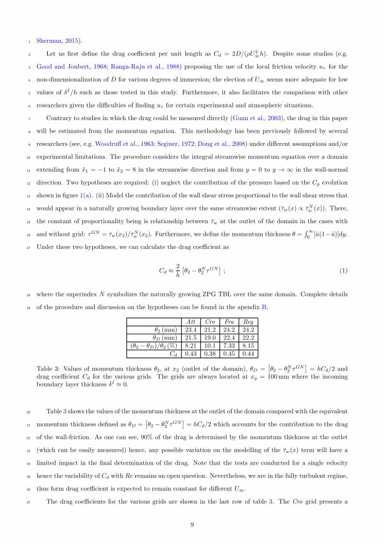
Figure 3: Profiles of inner-scaled turbulence level u′+rms for various grids and streamwise locations. The grids
are always located at xg = 100mm where the incoming boundary layer thickness δI ≈ 0. The solid pink likeshows the approximate location of the outer peak related with the shear layer.
The previous section has characterized the bulk behaviour of the grids using their drag coefficient. Despite3
some differences for the Cro grid case, drag seems to be primarily determined by the porosity whereas its4
distribution plays a secondary role. However, the turbulence characteristics are more likely to be influenced by5
the different grids’ bars orientation and geometry. This section will show the one-point statistics and turbulence6
level in the lee of the various grids.7
Figure 3 shows the profiles of u′
rms for the various grids and streamwise locations. No correction is applied8
to mitigate the effect of limited spanwise resolution (downstream of the grids uτ is smaller than in the natural9
case, hence l+w is also smaller and the resolution is improved). As a consequence, the peak turbulence intensity10
(at y+ ≈ 15) increases slightly with streamwise distance for every case.11
It seems logical to assume that the disturbed rms velocity profiles in the closest location to the grid will12
evolve with x until a closer resemblance to the natural case is achieved; indeed this situation is observed for13
every grid. In the closest measurement station (x = 9) the profiles qualitatively follow the natural case in the14
inner region (y+ / 300) whereas they display a clear departure further from the wall. A large peak is found15
in the external layer collapsing at y = 1 ↔ y+ ≈ 2000 which is most likely due to the shear layer appearing16
between the grids’ wake and the freestream. This peak decreases in magnitude with x; simultaneously, the17
rms level in the region 300 / y+ / 1000 increases with x for every grid. The interaction between the inner18
11
region and the grids’ wake may have some similarities with a TBL flow developing under freestream turbulence.1
However, in the present case the shear layer also presents some influence in the near-wall region which would2
not be the case under freestream turbulent conditions. This topic will be further discussed in section 3.3.3
Although the grids’ wakes generate a highly turbulent fluid in their vicinity, these wakes meet and interact far4
upstream of the first measurement station where their turbulence intensity is significantly smaller. Turbulence5
decay downstream of single- and multi-scale grids has been broadly documented before (see, for instance Hurst6
and Vassilicos, 2007; Mazellier and Vassilicos, 2010). Considering the turbulence intensity downstream of grid-7
generated turbulence, the turbulence level is reported to increase with the streamwise coordinate before reaching8
a peak at x ≈ 0.4x⋆; the turbulence intensity subsequently decreases further downstream. The definition of9
x⋆ = L20/t0 as a relationship between the length and thickness of the largest bar appears when considering the10
meeting point of these bars’ wakes. For the grid presenting the largest x⋆ = L20/t0 = 650mm (Fra) and in11
the closest measurement point we have x = 9 ↔ x = 1.23x⋆; which is far downstream of the peak appearance.12
Contrastingly, the turbulence level of the shear layer is maintained significantly higher much further downstream,13
probably as a consequence of the high shear which sustains the turbulence production (see figure 5 and the14
discussion below).15
102 103 104
λ+x
0
0.5
1
1.5
2
E11f/u2 τ
Att
x = 9 x = 15 x = 19 x = 25 x = 31 x = 43
102 103 104
λ+x
Cro
102 103 104
λ+x
Fra
102 103 104
λ+x
Reg
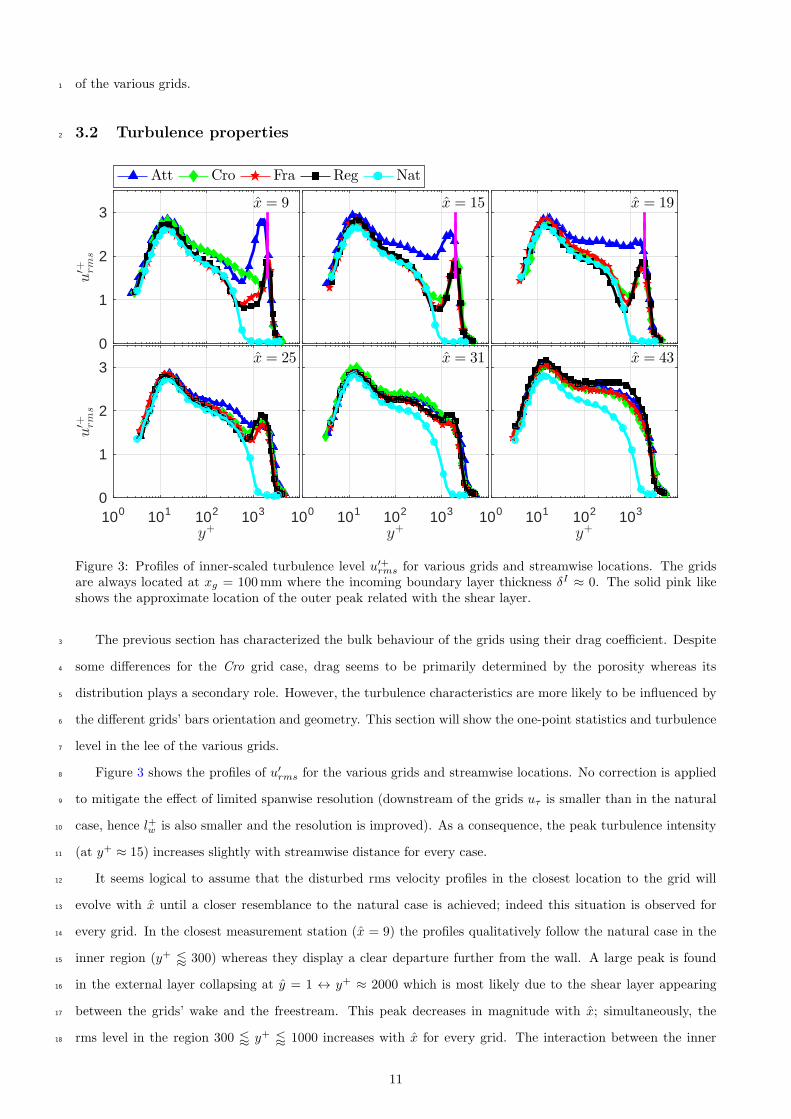
Figure 4: Inner-scaled premultiplied spectra, E11(u′)f/u2
τ , as a function of inner-scaled length scale, λ+x , at
y+ = 15 for various grids and streamwise locations. The grids are always located at xg = 100mm where theincoming boundary layer thickness δI ≈ 0.
Summarizing, figure 3 at x = 9 shows an inner region (y+ / 300) largely influenced by the presence of16
the wall and its mechanism of turbulence production for all grids; a second layer (300 / y+ / 2000) related17
to the grids’ bars’ wakes which presents a lower intensity as a consequence of their progressive decay and a18
strong external peak related to the shear layer appearing above the grid. Further downstream, the different19
layers progressively mix with each other until a qualitative resemblance to the natural case is obtained. Further20
explanation can be sought in the study of the spectral content of the streamwise velocity fluctuations. If the21
inner region is actually dominated by the presence of the wall, then its spectra would be expected to resemble22
that of a natural TBL in this region.23
Figure 4 shows the spectral content of the fluctuations for different grids and streamwise locations at y+ = 15,24
i.e. the location of the inner peak of turbulent intensity. The spectra are plotted against the inner scaled length25
12

scale λ+x = λxuτ/ν = u15uτ/(fν), where the transformation from frequency to length has been performed based1
on Taylor’s hypothesis considering the mean velocity u15 = u(y+ = 15) at the inner peak location. It is clearly2
observed that the spectral energy at the inner peak is primarily concentrated around λ+x ≈ 1000. This effect has3
been broadly reported before as representative of the inner behaviour of natural TBLs (see e.g. Chernyshenko4
and Baig, 2005b; Marusic et al., 2010; Rodrıguez-Lopez et al., 2016b). Note that the use of Taylor’s hypothesis5
in spatially evolving flows may be challenged; however, figures 3 and 4 show that the behaviour in the inner6
region seems to closely resemeble that of a natural TBL, hence the derivatives in the streamwise direction may7
be assumed to be sufficiently small so that Taylor’s hypothesis may still be applied as commonly done in natural8
TBLs (e.g. Marusic et al., 2010).9
0
0.5
1
1.5
y
x = 9
δs
x = 15
δs
x = 19
δs
0.2 0.4 0.6 0.8 1
u
0
0.5
1
1.5
y
x = 25
0.2 0.4 0.6 0.8 1
u
x = 31
0.2 0.4 0.6 0.8 1
u
x = 430.2 0.4 0.6 0.8
y/δ99
0
4
8
12(U∞ − u)/uτ
Att Cro Fra Reg Nat
0.2 0.4 0.6 0.8y/δ99
0
4
8
12(U∞ − u)/uτ
0.2 0.4 0.6 0.8y/δ99
0
4
8
12(U∞ − u)/uτ
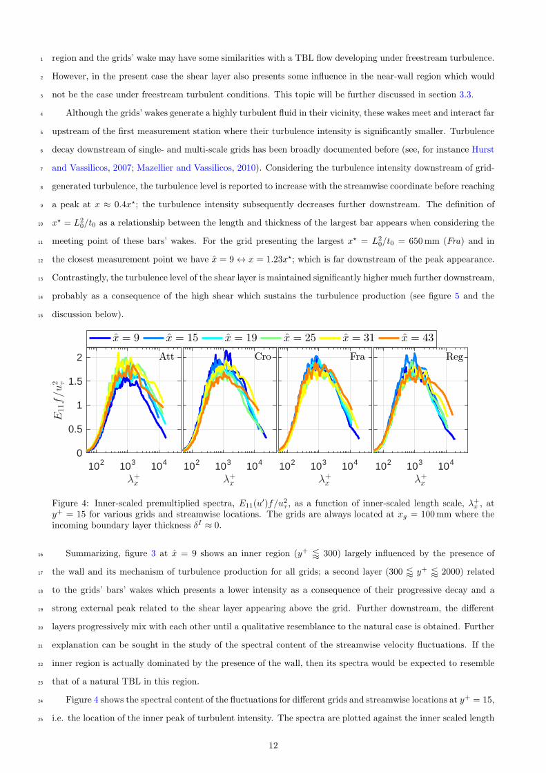
Figure 5: Wall-normal profiles of outer-scaled mean velocity u for various grids and streamwise locations. Thedashed red lines in the upper three plots show the linear trends fitted to the shear layer along with their thicknessδs, for the Fra grid. The insets in the bottom row show the outer-scaled velocity defects profiles for the variousgrids. The grids are always located at xg = 100mm where the incoming boundary layer thickness δI ≈ 0.
In order to assess the relationship of the outer peak with the shear layer, one should compare its wall-normal10
extent with the thickness of the shear layer δs. This thickness can be measured from the mean velocity profile11
by fitting a straight line in the vicinity of y = 1 (the central point of the shear layer). The point at which the12
mean velocity profile departs from the linear trend by a specified threshold (arbitrarily taken to be 0.02U∞) is13
defined as the lower limit of the shear layer which extends until δ99. Consequently, the distance between these14
two points is the thickness δs. This is shown in figure 5 where the streamwise evolution of the mean profiles15
is studied. Whilst for the sake of brevity, the linear fit in the shear layer is only shown for the Fra grid; no16
qualitative changes are observed for the other grids. As expected, the thickness of the shear layer increases17
with the streamwise coordinate and, similarly, the intensity of the shear (du/dy) decreases with x. For x > 2418
13

the shear layer cannot be further distinguished which is consistent with the disappearance of the associated1
turbulence intensity peak for the same streamwise locations (c.f. figure 3).2
Velocity defect profiles are shown in the insets of figure 5 once the shear layer has lost its predominant effect3
(i.e. x > 24). Whilst the lack of collapse with the natural case is not surprising, there is a certain tendency for4
the velocity profiles downstream of the various grids to resemble the natural case more closely for increasing x.5
In essence, it seems reasonable that eddies in the outer region (scaling in outer units) need a longer streamwise6
distance (in physical units) to recover than significantly smaller scales near the wall (scaling in viscous units).7
This may be related with a larger turnover time associated with scales of the order δ99 rather than near-wall8
structures scaling with viscous units.9
Att
102 103 104
λ+x
0
0.5
1
1.5
y
0 0.5 1 1.5 2 2.5 3E11f/u2τ
Cro
102 103 104
λ+x
Fra
102 103 104
λ+x
Reg
102 103 104
λ+x
Figure 6: Inner-scaled premultiplied spectra, E11(u′)f/u2
τ , as a function of inner-scaled length scale, λ+x , and
the wall-normal coordinate y for various grids and x = 9. Solid lines show the thickness of the shear layer δsand dashed lines are provisionally sketched separating inner and shear layers. The grids are always located atxg = 100mm where the incoming boundary layer thickness δI ≈ 0.
Figure 6 shows the wall-normal contours of premultiplied spectra E11(u′)f/u2
τ , as a function of inner-scaled10
length scale, λ+x at the first measurement station (x = 9). The scaling of the inner peak is solely influenced11
by the wall with a concentration of spectral energy around λ+x ≈ 1000 as confirmed in figure 4. The outer12
peak appearing in the u′
rms profiles is also clearly present in the spectral contours. Moreover, its wall-normal13
position and extent correspond with the thickness of the shear layer δs estimated as described above. Note that14
δs is defined by means of the departure from a linear trend in the mean profile and it is a valid scaling for the15
size of the spectral peak. This establishes a link between the shear in this region (which entails an enhanced16
production level) and the spectral content. For every grid, it is also clear that the intermediate region between17
the inner and outer peaks contains a much smaller turbulent kinetic energy as a consequence of the grids’ wake18
having decayed much faster in the absence of any mean shear which sustains the turbulence production.19
Special mention is required for the Att grid which, as opposed to the other three, shows a broader peak20
in the shear layer with a larger energy content which also extends for a greater wall-normal extent. This is21
probably due to a combination of much thicker vertical bars and open gaps whose interactions enhance the22
turbulent activity in the shear layer of this grid. Contrastingly, Fra and Reg grids present a narrower peak23
in the shear region which is undoubtedly separated from the near-wall region. This result could be predicted24
14

by looking at figure 3 in x = 9 where the rms profiles for these two grids exactly follow the natural case for1
y+ < 300 as opposed to the Att case and, to a lesser extent, the Cro for which there is a larger departure.2
The large wall-normal extent and energy content of the shear layer for the Att grid may influence the near-wall3
behaviour in a different way than the other two grids. In fact, this was reported in Rodrıguez-Lopez et al.4
(2017) where the Att grid was observed to present up to a 10% larger wall shear stress fluctuations (τ ′+w,rms)5
than that predicted at a comparable Reynolds number. This effect is likely due to the enhanced interaction6
between inner and outer layers as a consequence of its larger energy content.7
As opposed to the other 3 grids, Cro case presents a larger energy content in the region 0.2 ≤ y ≤ 0.6.8
Although this extra energy seems to be relatively independent from the shear layer; it may be assumed that it9
does not come from the wall either (the small streamwise location, x = 9, makes it unlikely for the boundary10
layer to have grown up to y ≈ 0.6). Hence it seems logical to hypothesize that, for the Cro case, the grid’s wake11
persist for a longer streamwise distance or, at least, presents a larger influence in the near-wall region. This may12
have some implications on other results, for instance, Rodrıguez-Lopez et al. (2016a) related a larger influence13
of the wake on the wall with the presence of negative wall-normal velocities. This was previously hypothesized14
in section 3.1 as a candidate for explaining the slightly different value of Cd in the Cro case.15
Summarizing, the spectral content and rms profiles provide enough evidence to suggest the appearance of16
two well-differentiated layers: (i) a wall layer as a consequence of the interaction with the wall and (ii) a second17
region related with the shear layer appearing between the grid and the freestream with a large turbulence18
activity due to the production facilitated by the high mean shear. Furthermore, one can tentatively sketch a19
qualitative separation between these two layers where the spectral contours are narrower (or even disappearing20
such as the Reg case). This separation is shown in figure 6 with a horizontal dashed line. Section 3.3 will21
propose a systematic method to establish a way to measure the separation between these layers which may have22
some implications for boundary layer scaling.23
3.3 Two layers concept24
The appearance of two layers inside the TBL such as those characterized in section 3.2 has been previously25
reported by different authors. One example of these layers, appears downstream of a sudden change in surface26
roughness. In these cases two layers are usually differentiated: one layer located far from the wall (whose prop-27
erties are set by the rough upstream boundary conditions) and a second region located close to the wall (with28
properties set by the roughness condition dowstream of the sudden change). With the streamwise distance, this29
second region progressively grows by mixing with the outer one in order to adapt to the new boundary condi-30
tion. Several examples can be found to establish a well-defined border between these two layers: for instance,31
Andreopoulos and Wood (1982) propose successive streamwise differentiation of velocity profiles. Contrarily,32
Antonia and Luxton (1971) showed that the border between these two layers could be characterized by an33
inflection in the profile u ∝ √y. More recently, this procedure was employed by Hanson and Ganapathisub-34
ramani (2016) who additionally proposed different velocity scalings for the inner and outer layers. A further35
15

methodology is proposed by Efros and Krogstad (2011), who fitted straight lines to the u′+rms profiles.1
Apart from studies considering step changes in surface roughness; the appearance of two well-differentiated2
layers has also been identified in TBLs subject to freestream turbulence (Dogan et al., 2016) or evolution from3
strong tripping conditions (Rodrıguez-Lopez et al., 2016a). In this case, Rodrıguez-Lopez et al. (2016a) who4
defined the border between them based on a drop in the correlation level with the near-wall region below a5
certain threshold.6
The main objective of this section is to propose and validate a method being able of distinguish between7
these two regions such that it should establish a clear border between them. Furthermore, it is conjectured8
that the thickness of the inner layer would act as an effective “outer scale” for the pseudo-TBL development9
underneath and therefore several quantities could be found to scale with this thickness. A qualitative sketch of10
the two layers is presented in figure 7(a). For completeness, the shear layer and its thickness δs described in11
section 3.2 are also sketched.12
However, none of the aforementioned methods of internal layer detection can be applied, essentially because13
the flow configuration is radically different. An alternative method therefore is proposed which can be applied14
to the present flow. Given that the appearance of the two layers has been postulated by studying the velocity15
fluctuations and spectral profiles, a deeper study of the u′+rms profile seems appropriate. In fact, note that these16
profiles (for the Fra and Reg cases) follow the natural TBL trend with surprising accuracy, despite the much17
lower Reynolds number of this case. This suggests that, in essence, one could look for a natural boundary layer18
of a Reynolds number smaller than the Grid+TBL case which presents the same u′+rms profile in the inner region.19
However, this procedure (finding a natural case that resembles the measured profile close to the wall) requires20
an underlying assumption that may be contradictory, namely, it neglects the influence of the outer region on21
the inner layer. Whilst there is experimental evidence showing that this interaction does exist (especially the22
influence of freestream turbulence on TBLs); we might neglect it as a first approach according to the results23
presented in figure 6. One can easily observe that there is indeed a much larger separation, at least for the Fra24
and Reg cases, than the typical interaction between freestream turbulence and TBLs (see, for instance Dogan25
et al., 2016). On the other hand, some problems may be foreseen in the Att and Cro cases due to the insufficient26
separation of layers or an excessive influence of the outer layer in the near-wall region (c.f. figure 6).27
Symbol Reference min Reτ max Reτ Points Type
OS13 ◭ Orlu and Schlatter (2013) 794 2017 14 Exp (HW)DE00 N Degraa et al. (1999) 541 10023 5 Exp (LDV)
HNMC09 ◮ Hutchins et al. (2009) 2820 18830 5 Exp (HW)RBB16 H Rodrıguez-Lopez et al. (2016b) 285 1058 7 Exp (HW)SJM13 ♦ Sillero et al. (2013) 1307 1989 6 DNS
SO10 � Schlatter and Orlu (2010) 252 1271 10 DNSDLV17 ⋆ Dıaz-Daniel et al. (2017) 400 650 6 DNS
Table 4: Summary of experiments (Exp) and direct numerical simulations (DNS) used to fit the expressionu′+rms = f(Reτ) given by equation (2).
16

(a)
102
103
104
Reτ
0.8
1
1.2
1.4
1.6
1.8
2
2.2
2.4
2.6
u′+ rm
s| y
+=200 OS13
DE00
HNMC09
RBB16
SJM13
SO10
DLV17
(b)
Figure 7: (a) Sketch of the δeff concept, the boundary layer properties are only influenced by the wall layersetting δeff or δρ as the typical length scale. (b) Compilation of u′+
rms at y+ = 200 for different experiments(filled triangles) and DNS simulations (empty symbols); see table 4 for the interpretation of the legend. Theblack dots show the Reτ for Reg grid at various x based on δ99 and the green dots show their correspondingReeff = δeffuτ/ν. The solid line is the empirical fitting given by equation (2) and the dashed lines show the95% confidence interval.
3.3.1 δeff definition1
δeff is defined as the thickness of an hypothetical natural TBL which would provide the same level of u′+rms2
in the wall layer of the Grid+TBL cases. The first problem to consider is which wall-normal extent should be3
compared with the natural case. The very near-wall region (buffer layer and below) is uniquely determined by4
the presence of the wall and its boundary condition, hence a resemblance with the natural case is expected and5
very little information could be extracted from this fact. Therefore, comparison with the natural case should6
be sought further away from the wall and y+ = O(100) seems a good starting point.7
The procedure is shown in figure 7(b) and described as follows: (i) compile the values of u′+rms at y+ =8
100, 200, 300 for several experiments and direct numerical simulations covering two decades of Reτ (blue and9
red symbols in figure 7(b)). (ii) fit an analytical expression u′+rms|y+=i = fi(Reτ ) with i = 100, 200, 300 (solid10
black line in figure 7(b)). (iii) Use the measured level of u′+
rms,i at the three wall normal locations to find Reeff,iτ11
such that u′+
rms,i|y+=i = fi(Reeff,iτ ). As shown in figure 7(b) with black dots the Reynolds number based on δ9912
does not capture the phenomena hence we find the “effective” Reynolds which should have the same level of13
fluctuations at that particular y+ (i.e. the green dots in figure 7(b)). (iv) The effective Reynolds number would14
be the average between the results obtained at the three wall-normal locations (Reeffτ =∑
Reeff,iτ /3). (v)15
Thus the thickness of the inner layer (so-called effective thickness) would be δeff = Reeffτ ν/uτ . The functional16
form of fi(Reτ ) is postulated as17
u′+rms|y+=i = AiReτ +Bi logReτ + Ci
logReτReτ
, (2)
where the selection of the functional form is not intended to provide any physical explanation of the phenomena18
involved. The functional dependence proposed by Marusic and Kunkel (2003) could not be employed since it is19
17

applicable only for wall-normal positions farther from the wall (y+ > 300). Furthermore, scaling based on the1
diagnostic plot (Alfredsson et al., 2011) was avoided since it does not provide any direct relationship with the2
boundary layer thickness.3
Figure 7(b) shows one example of this procedure (Reg grid at y+ = 200), other examples are similar and4
they are not shown for brevity. In this figure, one can observe the accurate fit provided by equation (2) to the5
various experiments and simulations of natural TBLs. Note that no correction for limited spanwise resolution6
has been applied to any data since this effect is expected to be negligibly small at y+ > 100 (Hutchins et al.,7
2009). Note also that, due to the lack of experimental data at very high Reτ , the uncertainty (given by the8
95% confidence interval) in this region is larger. This may present a problem for the furthest x locations of9
the experiment where Reeffτ → Reτ = δ99uτ/ν ≈ 3000. The solid black dots in figure 7(b) show the Reynolds10
number based on δ99; whereas the green dots show the value of Reeffτ estimated from the measured level of11
u′+rms. It is clearly observed that the original value of Reτ is not the correct one for scaling the turbulence12
intensity at this point.13
3.3.2 δρ definition14
Alternatively, one can follow the methodology proposed by Rodrıguez-Lopez et al. (2016a) who defined the15
wall layer as the region in which the correlation of the streamwise velocity fluctuations with a point located16
in the buffer layer was larger than a certain threshold ρ⋆uu = 0.3. Analogously, two-point streamwise velocity17
correlations were performed as described in section 2.3. The wall hot wire was located at a fixed point (x0, y+
0 ≈18
4, z0) and the free hot wire was traversed in the wall-normal direction for the same x0 and z0. To account19
for the inclination of the turbulent structures a time delay η, between the two signals was applied following20
extensive experimental evidence (Brown and Thomas, 1977; Robinson, 1986; Boppe et al., 1999; Marusic and21
Heuer, 2007). In these conditions the correlation factor can be defined as22
ρuu(y) =
∫
∞
0u′
whw(y0, t+ η)u′
fhw(y, t)dt
u′
whw,rmsu′
fhw,rms
. (3)
The point y⋆ at which ρuu(y⋆) < ρ⋆uu = 0.3 can be taken as representative of the inner layer. For a natural23
boundary layer this occurs at approximately y/δ ≈ 1/8 (scaling with outer units, see e.g. Marusic and Heuer,24
2007; Rodrıguez-Lopez et al., 2016b; Dıaz-Daniel et al., 2017). Since the objective is obtaining the thickness of a25
natural boundary layer which would exhibit similar near-wall behaviour, we can define an alternative definition26
of the effective thickness as δρ = 8y⋆, where the subindex ρ symbolizes that it has been obtained from the27
wall-normal profiles of streamwise correlation. The factor of 8 is dependent on y0, the wall-normal position of28
the WHW. Note however, that it does not play any role concerning the validity of δρ as a scaling parameter29
since this is invariant to any multiplicative constant.30
18

10 20 30 40x
0
0.5
1
1.5
2
2.5
3δ/δ 9
9
Att
10 20 30 40x
Cro δ99δρδeffNat
10 20 30 40x
Fra
10 20 30 40x
Reg
Figure 8: Evolution of the effective thickness δeff (with 95% confidence bounds) and the thickness based onthe correlation level δρ for various grids. The grids are always located at xg = 100mm where the incomingboundary layer thickness δI ≈ 0. The solid light-blue line shows the value of the natural TBL thickness (δNat
99 )for the various streamwise locations.
3.3.3 δeff and δρ evolution1
Figure 8 shows the streamwise evolution of these two definitions of effective thickness for the various grids2
tested. The 95% confidence interval in the determination of δeff (the two solid thin lines in figure 8) is the3
same as shown in figure 7(b). This is larger for high Re since there are less experiments at these conditions.4
Furthermore, the logarithmic trend of the curve in equation (2) makes it harder to extrapolate large Reeffτ5
from the turbulence intensity profile. The agreement between the two definitions of the inner layer thickness is6
clear and therefore it suggests the appearance of a well-defined physical mechanism in this region. The overall7
behaviour for all the grids is as expected, δeff is much smaller than δ99 close to the fences and grows by mixing8
with the grids’ wake and the shear layer until all the turbulent flow interacts with the near-wall region in the9
same manner as a TBL would do. The fact that δeff or δρ can be larger than δ99 for the furthest streamwise10
locations may be possible because of the influence of the turbulent outer fluid. In fact, a similar effect is11
observed for TBLs developing under the influence of freestream turbulence (Dogan et al., 2016) where certain12
properties of the TBL (such as the departure from the logarithmic law) are shown to be representative of a13
thicker boundary layer. Essentially, the same trend is observed here (especially for the Att grid), due to the14
large energy in the outer part of the TBL, the near-wall region behaves as a natural TBL which would have a15
thickness larger than δ99. Therefore these methods, present the potential of detecting not only the thickness of16
the wall layer but also the effective thickness generated as a consequence of an enhanced influence of the wake17
into the near-wall region.18
To summarize, after the identification of two differentiated layers in the grid+TBL flow in section 3.2; this19
section has presented two systematic procedures by which one can establish the thickness of the inner layer20
based on the u′+rms profile (δeff ) or the wall-normal variation of streamwise velocity correlation (δρ).21
19

3.4 Scaling of wall shear stress fluctuations1
The first test that these scalings should fulfil is the correct determination of the behaviour near the wall. A2
possible way to assess this behaviour is by means of the fluctuating wall shear stress τ ′+w,rms (Schlatter and Orlu,3
2010, 2012). This is shown to present a logarithmic trend with Reτ (which depends on the thickness of the4
boundary layer), hence it has potential as a diagnosis quantity for this new scaling. Rodrıguez-Lopez et al.5
(2017) obtained the fluctuations of the wall shear stress by means of a wall-mounted hot wire located in the6
inner region. This hot wire was calibrated against a naturally growing TBL where the wall shear stress can7
be extrapolated from the mean velocity profile as shown in Rodrıguez-Lopez et al. (2015). They showed that8
τ ′+w,rms in the wake of these porous fences presents an adaptation region in which τ ′+w,rms was significantly lower9
than the predictions, followed by a tendency to recover the expected value. The hypothesis is that only the10
inner layer (of thicknes δeff or δρ) contributes to those fluctuations. From there, it follows that the so-called11
adaptation region in Rodrıguez-Lopez et al. (2017) was just the growth of the inner layer which progressively12
resembles δ99 with the streamwise distance as shown in figure 8. This is therefore consistent with a two-layer13
structure in which the wall layer grows with x until the resemblance of a TBL since Reeffτ → Reτ for large x.14
Figure 9 presents the same results of τ ′+w,rms but now scaled with the effective thickness of the inner layer15
calculated by the aforementioned procedures. The first result is the small dispersion appearing between δeff16
calculated at the three wall-normal locations. This result is satisfactory since it ensures that the correct flow17
phenomena are captured at various wall-normal locations. Furthermore, it is strikingly clear that the so-called18
adaptation region from the grids’ disturbances presents a well-defined scaling and it is not just a simple arbitrary19
transient process to adapt to the new boundary conditions. Similarly, the thickness of the wall layer obtained20
by means of the correlation level also presents a clear agreement with δeff (as could be anticipated by their21
similarity in figure 8). Moreover, it is also a valid scaling parameter for the wall shear stress fluctuations. A side22
note is required for the Att case. The new scaling significantly improves the data’s trend (τ ′+w,rms ∝ logReeffτ ).23
However, the values appear to be shifted by a constant of approximately 0.025 with respect to the prediction24
of Schlatter and Orlu (2010). It is hypothesized that this could be related with the extraordinarily high25
intensity of the shear layer peak (discussed above in section 3.2) which enhances the fluctuations in the near-26
wall vicinity above the expected natural trend. However, the fact that the new scaling recovers the correct27
trend (τ ′+w,rms ∝ logReτ ) supports the use of this novel scaling for disrupted boundary layers.28
Whereas the correlation proposed by Schlatter and Orlu (2010) (based on DNS data, exempt from any29
measurement bias) is τ ′+w,rms = 0.298 + 0.018 logReτ ; Mathis et al. (2013) proposed shifting it by a constant30
τ ′+w,rms = 0.245 + 0.018 logReτ to account for a damping in the fluctuations due to the interaction between31
the hot-wire thermal wake and the wall substrate (Brunn, 1995; Chew et al., 1998). This attenuation appears32
independently of spanwise resolution effects (which are corrected in the present measurements as shown in33
Rodrıguez-Lopez et al. 2017). In any case, τ ′+w,rms = A + B logReτ can be interpreted as a constant level of34
fluctuations (likely caused by the presence of streaks Chernyshenko and Baig 2005a) plus a weak influence of the35
outer fluid (scaling with logReτ ). It has been reported that this interaction can be generated by a superposition36
20

103 104
Reτ
0.36
0.38
0.4
0.42
0.44τ′+ w,rms
Att
δ99 δy+=100eff δ
y+=200eff δ
y+=300eff
δρ 0.245 + 0.018 logReτ
103 104
Reτ
Cro
103 104
Reτ
Fra
103 104
Reτ
Reg
Figure 9: Wall shear stress fluctuations, τ ′+w,rms, as a function of Reτ based on different definitions of δ forvarious grids and streamwise locations. Data is taken from Rodrıguez-Lopez et al. (2017). Solid lines showτ ′+w,rms = 0.245 + 0.018 logReτ with 2% and 5% margins. The grids are always located at xg = 100mm where
the incoming boundary layer thickness δI ≈ 0.
and a modulation of the small near-wall structures by the large scale turbulence in the logarithmic layer (e.g.1
Mathis et al., 2011). Recovering τ ′+w,rms ∝ logReτ suggests that the physics of the flow in terms of the outer-2
inner interaction are captured by the scaling but the intensity of this effect is underestimated. This could be3
a consequence of a distinct influence of the grid’s wake on the wall region as hypothesized in section 3.2. An4
alternative interpretation of the distinct behaviour of Att grid could be given by the procedure described in5
Hanson and Ganapathisubramani (2016). In it, they specify a distinct velocity scale for the wall layer rather6
than uτ which would then recover the trend proposed by Schlatter and Orlu (2010). However this would be at7
odds with figures 3 and 4 which show uτ to be an adequate scaling for the location and magnitude of the inner8
turbulence peak. It also seems reasonable to assume that the skin-friction fluctuations scale with the local shear9
rather than with an outer-scale velocity such as U∞.10
By recovering the expected trend of τ ′+w,rms, this section has shown that the effective thickness of the inner11
layer is valid as an outer scaling for the pseudo-TBL developing underneath grid generated turbulence. The12
appearance of this scaling poses new questions regarding its applicability to other outer-scaled TBL phenomena.13
The next sections therefore will study the different length scales present in the flow and how their evolution can14
be explained in terms of this new scaling.15
3.5 Integral length scale, L1116
After having set the basis for the new scaling based on δeff , this section will study the wall-normal profiles of17
integral length scale and how their scaling may differ from that of a natural TBL. The longitudinal integral18
length scale L11 is obtained from single-component single-point hot-wire anemometry by considering the integral19
time scale T11 and the convection velocity uc: L11 = T11uc. Several studies have been focused on obtaining20
a value for the mean convection velocity across the TBL (Del Alamo and Jimenez, 2009; Geng et al., 2015)21
concluding that one can consider as a first approach the mean velocity profile uc = u(y) (i.e. Taylor’s hypothesis)22
for wall-normal positions such that the mean velocity is u+ & 11. Considering the autocorrelation function23
21

ρuu(η) =(∫
u′(t)u′(t+ η)dt)
/(u′2rms), one can obtain T11 by numerical integration of ρuu(η). In order to1
avoid the noise appearing at low ρuu, or equivalently, large time delays η, one can fit an exponential decay for2
ρuu < 0.5. Calculation of T11 based on Fourier spectra (not shown) provided qualitatively the same results.3
10-3
10-2
10-1
100
y/δ99
0
0.2
0.4
0.6
0.8
L11/δ 9
9
Att
x = 9 x = 15 x = 19 x = 25 x = 31 x = 37 x = 43
10-3
10-2
10-1
100
y/δeff
0
0.2
0.4
0.6
0.8
1
1.2
1.4
L11/δ e
ff
Att
10-3
10-2
10-1
100
y/δρ
0
0.2
0.4
0.6
0.8
1
L11/δ ρ
Att
10-3
10-2
10-1
100
y/δ99
Cro
10-3
10-2
10-1
100
y/δeff
Cro
10-3
10-2
10-1
100
y/δρ
Cro
10-3
10-2
10-1
100
y/δ99
Fra
10-3
10-2
10-1
100
y/δeff
Fra
10-3
10-2
10-1
100
y/δρ
Fra
10-3
10-2
10-1
100
y/δ99
Reg
10-3
10-2
10-1
100
y/δeff
Reg
10-3
10-2
10-1
100
y/δρ
Reg
Figure 10: Profiles of integral length scale L11, for various grids and streamwise locations normalized with δ99(first row) and with δeff (second row) and δρ (third row). The grids are always located at xg = 100mm wherethe incoming boundary layer thickness δI ≈ 0.
The first row of figure 10 shows the profiles of L11 scaled with δ99. Note that δ99 includes the three-layer4
structure described above, namely, wall layer, grid wake and shear layer. However, the typical length scales5
in the near-wall region should be expected to scale with the thickness of the wall layer rather than with δ99.6
Consequently, no collapse is observed in the first row of figure 10 for any grid or streamwise location. If, in the7
contrary, we use a scaling which accounts only for the thickness of the wall layer, that is, δeff or δρ as proposed8
above. Then L11 is shown to collapse when scaled with those parameters in the near wall region (second and9
third rows of figure 10 for y/δ / 0.2). Logically, this scaling is not valid out of the wall layer since it does not10
capture the physics there, which do not depend on the thickness of the near-wall region.11
A few differences can be observed between the two proposed scaling parameters. For cases where the12
22

spectral separation of scales is less clear (Att and Cro grids), L11 seems to scale better with δρ rather than1
δeff . This is likely due to the methodology followed to obtain δeff which relies on a sufficient separation of the2
spectral behaviour. Contrastingly, for cases where the separation in the turbulence intensity profiles is larger,3
the definition of δeff provides a better collapse. Independently, note that both δeff and δρ are more valid as a4
scaling parameter for the outer region of the wall-bounded flow than δ99 which does not reflect the separation5
between the wall and wake layers.6
For Fra and Reg cases the furthest streamwise location (x = 43) presents a distinct behaviour when scaled7
with δeff . Note that this is likely due to the large uncertainty in the determination of δeff for large Reτ values.8
In fact, figure 8 has shown that the point located at x = 43 presents an uncertainty of approximately 50%9
which, in turn, translates into a dubious scaling for the last point. If, on the other hand, we consider smaller10
streamwise locations (or, equivalently, Reynolds numbers), the collapse is shown to hold up to y/δeff of order11
unity.12
Note also that Att case presents as good a collapse as Fra and Reg grids despite its differences in terms13
of τ ′+w,rms (c.f. figure 9). In fact, Rodrıguez-Lopez et al. (2017) reported that, despite its larger τ ′+w,rms value,14
the autocorrelation of the wall shear stress for the Att grid was dominated by the presence of streaks (as in15
the natural case). This fact could be linked with the recovery of the trend τ ′+w,rms ∝ logReτ which was also16
related with the presence of streaks. In light of this evidence, it seems reasonable to hypothesize that the large17
turbulent kinetic energy in the outer part of the Att grid’s wake (generated by the combination of wakes of thick18
bars and large open areas) modifies the near-wall region by modifying its upper boundary condition. That is,19
the flow in the wall region, characterized by δeff , perceives the wake of the grid as its upper limit rather than20
the freestream. Since in this particular grid, the wake is more highly energetic (c.f. for instance, figure 6), the21
fluctuations are enhanced. However, the formation mechanisms of turbulence in the wall region (streaks) and22
its length scales remain unaltered. In essence, this mechanism would be equivalent to an inner boundary layer23
of thickness δeff in which the apparent freestream is modified by the presence of the grid’s wake enhancing24
turbulent fluctuations in a broadband manner, thus not modifying the predominant L11.25
To summarize, the integral length scale has been obtained from the correlation function and Taylor’s hy-26
pothesis showing that for a natural TBL it collapses in the inner region followed by a plateau with a Reynolds27
trend in the outer region. For the disrupted cases, δ99 cannot be used as a scaling parameter since it does not28
reflect the physics of the flow in the inner region which depend on its local thickness (determined either by δeff29
or δρ). Use of this scaling enables the collapse of L11 across the inner layer. For cases with insufficient spectral30
separation between the layers (Att and Cro grids as described in section 3.3), δρ presents a better collapse of31
the L11 profiles. Alternatively, if the spectral separation is larger (Fra and Reg grids) δeff is a better scaling32
parameter except for very high Reτ due to the larger uncertainty at the last position.33
23

3.6 Spanwise turbulent structure1
The streamwise characteristic lengths of the flow have been studied by means of L11 in section 3.5. However, the2
flow in the vicinity of a wall is strongly anisotropic in the spanwise direction. The spanwise organization of TBL3
flows in the near-wall region is characterized by the appearance of large or very large meandering structures4
resident in the logarithmic layer (e.g. Ganapathisubramani et al., 2005; Hutchins and Marusic, 2007a). These5
structures have also been reported to appear downstream of mild disruptions such as strong tripping conditions6
(Rodrıguez-Lopez et al., 2016b). Moreover, they also imprint their characteristics on the near wall region as a7
consequence of the inner-outer interaction mechanisms (Hutchins and Marusic, 2007b). As reported in Hutchins8
and Marusic (2007a), the spanwise separation of these structures clearly scales with the local boundary layer9
thickness. Hence it seems relevant to study their scaling under the influence of the grids’ wakes in terms of the10
new definitions of the internal thickness.11
0.1 0.3 0.5 0.7 0.9-0.2
0
0.2
0.4
0.6
0.1 0.3 0.5 0.7 0.9-0.2
0
0.2
0.4
0.6
0.1 0.3 0.5 0.7 0.9
0.1 0.3 0.5 0.7 0.9
0.1 0.3 0.5 0.7 0.9
0.1 0.3 0.5 0.7 0.9
0.1 0.3 0.5 0.7 0.9
0.1 0.3 0.5 0.7 0.9
0.2 0.6 1
0
0.25
0.2 0.6 1
0
0.25
0.2 0.6 1
0
0.25
0.2 0.6 1
0
0.25
0.2 0.6 1
0
0.25
0.2 0.6 1
0
0.25
0.2 0.6 1
0
0.25
0.2 0.6 1
0
0.25
Figure 11: Profiles of the spanwise correlation of streamwise velocity ρuu(z) at the beginning of the logarithmicregion, y+ ≈ 60, y/δ99 ≈ 0.02, (main plots) and in the near-wall region, y+ ≈ 4 (insets), for various gridsand streamwise locations normalized with δ99 (first row) and δρ (second row). The grids are always located atxg = 100mm where the incoming boundary layer thickness δI ≈ 0.
Two-point spanwise measurements are taken using both WHW and FHW simultaneously. Two heights over12
the wall are selected, one inside the very near-wall region y+ ≈ 4, which may be representative of the behaviour13
close to the wall and another one at the beginning of the logarithmic layer (y+ ≈ 60) where these very large14
24

structures are expected to appear. Correlation of the streamwise velocity in the spanwise direction is defined as1
ρuu(z) =
∫
∞
0u′
whw(z = 0, t)u′
fhw(z, t)dt
u′
whw,rmsu′
fhw,rms
(4)
where the minimum separation between the measurement points (given by the physical size of the hot wires) is2
approximately 4mm. A similar experimental arrangement was used in Rodrıguez-Lopez et al. (2016b).3
The first row of figure 11 shows the spanwise correlation of streamwise velocity for several grids and stream-4
wise locations normalized with δ99. The lack of collapse for different x is clearly observed, in particular, this5
effect is more pronounced closer to the grids. Note that, for x ≤ 15, ρuu drops to 0 for z/δ99 ≈ 0.05, much6
smaller than the expected value of approximately 0.3 (Hutchins and Marusic, 2007a). Furthermore, for Att and7
Cro grids, very little negative correlation is found for x < 24. This contrasts with the natural TBL case, in8
which the turbulent structures of positive fluctuation are flanked by negative ones. It seems therefore reasonable9
to assume that the presence of the grids destroys this pattern. This effect is less clear for Fra and Reg grids10
suggesting that the wall behaviour is less disrupted in this case, which is in agreement with past observations11
regarding the interaction between outer and wall layers (c.f. sections 3.2 and 3.3). Both effects (rapid loss12
in correlation and lack of negative values) tend towards the expected values of a natural TBL with x, this is13
consistent with the growth of the internal layer which progressively tends to δ99. In particular, the typical14
arrangement of alternating spanwise structures is recovered for Att and Cro grids at x ≈ 24, this is the same15
straemwise location where the turbulence peak related with the shear layer is lost (c.f. figure 3). From this16
evidence, it could be conjectured that the disappearance of the shear-layer peak and the appearance of the large17
structures in the logarithmic layer are related. Moreover, the geometry of the grids (figure 2) also suggests that18
Att and Cro grids should destroy the turbulent structures in the wall region more effectively as a consequence19
of the larger concentration of bars close to y = 0.20
Let us now normalize the spanwise separation with the new scaling thickness δρ as shown in the second row21
of figure 11. The performance of δeff as a scaling parameter is unsusprisingly worse, since δρ is based in the22
two-point correlation hence it is more valid to describe ρuu in other directions. Thus, for the sake of brevity23
only results scaled with δρ are presented.24
One can note that the collapse of Fra and Reg grids is significantly improved with respect to the degree of25
matching presented in L11/δρ (figure 10). The important result resides not only in the fact that the curves are26
shown to collapse amongst themselves, but also in the spanwise location of the minimum of the correlation, this27
is always located close to z/δρ ≈ 0.3 as has been reported for natural TBLs (Ganapathisubramani et al., 2005;28
Hutchins and Marusic, 2007a; Rodrıguez-Lopez et al., 2016b). Hence, this provides consistent evidence for δρ29
being the correct scaling for the wall layer forming under the grids’ wake.30
The spanwise organization present in the logarithmic layer shows its footprint in the near-wall region. This is31
shown in the insets of figure 11, where the same correlations are plotted but this time at y+ ≈ 4. The maximum32
correlation level is unsurprisingly smaller since the initial separation between the two hot wires is kept constant33
and typical eddy sizes are expected to be much smaller in this region than in the logarithmic layer (c.f. also34
25

figure 10). However, a similar trend is observed for all the grids and streamwise locations which collapse with1
δρ.2
Summarizing, large structures flanked by opposite sign fluctuations are destroyed in the vicinity of Att and3
Cro grids to form again after approximately 24 grid heights. For streamwise distances larger than this value4
and for the other two grids (at every x) these large structures are detected in the logarithmic layer with a5
separation of approximately 0.3δρ (analogous to a naturally developing TBL). As expected, it is shown that δ996
cannot be used as a scaling parameter, as it does not capture the physics of the wall layer. The footprint of7
these structures is also reflected in the very near-wall region with analogous separation (∝ δρ). This constitutes8
clear evidence of the dominant scaling in the wall layer.9
3.7 Incoming boundary layer influence10
Having established the dependence of TBL properties on the thickness of the inner layer, δρ or δeff , a question11
arises regarding the potential influence of the incoming BL thickness on the flow downstream of the grids. In12
particular, note that the scaling based on δeff was severely challenged in the Cro case, where the grid’s wake13
presented a larger interaction with the near-wall region. This influence was observed as a connection between14
the inner spectral peak and the shear layer region (c.f. figure 6). Moreover, it generated further difficulties for15
the determination of δeff from the u′+rms profile. It may be speculated that such scaling would exist even in this16
case but it cannot be detected with the present methodology. A similar effect (larger connection of the spectral17
contours between the inner and shear layers) can be obtained by the immersion of the grid in a progressively18
thicker TBL. This section therefore will study the spectra and integral length scale downstream of the various19
grids with different incoming TBLs.20
The different incoming boundary layers (of thickness δI and momentum thickness θI) are obtained by means21
of placing the grid at different streamwise locations where the TBL has grown to a larger thickness. All the22
measurements are taken at x = 8, i.e. 8 grid heights downstream of the grid. Five different degrees of immersion23
are tested ranging from virtually 0 (the case studied up until now) to approximately 80% of the grid height. For24
the thickest TBL case, artificial tripping was used to deliberately overtrip the developing TBL. This trip was25
made of two rows of slender cylinders 20mm high with their axis normal to the wall placed at 160mm from the26
leading edge. Details of this experimental arrangement can be found in Rodrıguez-Lopez et al. (2016b,a) where27
it is also justified that the TBL properties at the considered streamwise location are sufficiently canonical and28
the trip influence seems to be forgotten (at least sufficiently for the present purpose). Two different thickness of29
the TBL can be considered, δI99 based on the mean velocity profile reaching 0.99U∞ or, alternatively, δI based30
on a fit of a composite profile to the outer layer (Chauhan et al., 2009; Rodrıguez-Lopez et al., 2015). Table 531
summarizes the main parameters of the various incoming TBLs.32
Increasing the thickness of the incoming TBL implies that a larger fraction of the grid is subject to incoming33
turbulence (as opposed to the original case in which almost the whole flow impacting the grid was laminar).34
Furthermore, the length scale of the turbulence inside the incoming boundary layer will also increase (scaling35
26

xg δI99 (mm) δI (mm) θI (mm) Reθ uτ (ms−1) Reτ1 1 1.91 2.49 0.26 168 0.36 58
8 18.4 26.2 3.08 1891 0.40 68719 33.2 44.7 4.22 2623 0.37 106636 44.6 58.2 5.81 3563 0.38 1419
2 36 59.9 78.6 8.53 5220 0.36 1805
1: Estimation from Blasius laminar BL at x = 1.
2: With cylinders tripping based on Rodrıguez-Lopez et al. (2016b,a).
Table 5: Summary of TBL properties for various incoming TBL thickness. The friction velocity uIτ is extrapo-
lated from the mean velocity profile (Rodrıguez-Lopez et al., 2015).
with its thickness, c.f. figure 12(b)). This last effect is particularly important since it is anticipated that the1
grids interact with incoming turbulence of similar lengths to their mesh size (e.g. Groth and Johansson, 1988).2
Figure 12 shows the integral length scale for the various incoming boundary layers without the grid. Figure 12(b)3
follows the expected trend for the natural TBL exhibiting a collapse for small y followed by a plateau with a4
slight Reynolds trend. This fact entails that L11 grows with respect to the grid height (and consequently any5
measurement of the mesh size) as shown in figure 12(a). One can observe that there is a clear increase in both6
the fraction of grid influenced by the incoming TBL and also the typical length scale of this turbulence. Whilst7
the near-wall region is strongly influenced by the presence of the wall, the vast majority of the grids are exposed8
to turbulence of quasi constant L11.9
0 0.1 0.2 0.3 0.4 0.5L11
0
0.2
0.4
0.6
0.8
1
y
δI ≈ 0
δI = 0.26
δI = 0.45
δI = 0.58
δI = 0.79
(a)
10-3 10-2 10-1 100
y/δI99
0
0.2
0.4
0.6
0.8
1
L11/δI 99
(b)
Figure 12: Wall-normal profile of integral length scale L11, for different incoming boundary layers as a functionof y normalized with (a) the grid height h, and (b) the local TBL thickness δI99.
The increasing proportion of the grid influenced by the incoming turbulence can also be seen in the spectral10
contours. Figure 13 shows these contours for different incoming boundary layer thicknesses. The wall-normal11
extent of the region influenced by the near-wall turbulence is clearly seen to increase for larger incoming TBL.12
Furthermore, the dashed lines show the thickness of the incoming TBL (δI , based on mean-profile fitting)13
showing a clear correlation between the extent of the near-wall influenced region and the thickness of this layer.14
The behaviour of the other three grids is not shown for brevity but they show qualitatively similar trends.15
The intensity of the peak related with the shear layer is seen to increase with δI . This may be caused16
27
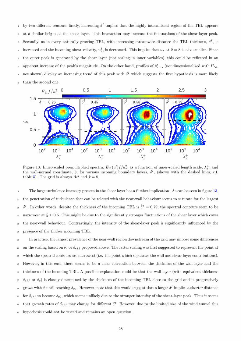
by two different reasons: firstly, increasing δI implies that the highly intermittent region of the TBL appears1
at a similar height as the shear layer. This interaction may increase the fluctuations of the shear-layer peak.2
Secondly, as in every naturally growing TBL, with increasing streamwise distance the TBL thickness, δI , is3
increased and the incoming shear velocity, uIτ , is decreased. This implies that uτ at x = 8 is also smaller. Since4
the outer peak is generated by the shear layer (not scaling in inner variables), this could be reflected in an5
apparent increase of the peak’s magnitude. On the other hand, profiles of u′
rms (nondimensionalized with U∞,6
not shown) display an increasing trend of this peak with δI which suggests the first hypothesis is more likely7
than the second one.8
δI = 0.26
102 103 104
λ+x
0
0.5
1
1.5
y
0 0.5 1 1.5 2 2.5 3E11f/u2τ
δI = 0.45
102 103 104
λ+x
δI = 0.58
102 103 104
λ+x
δI = 0.79
102 103 104
λ+x
Figure 13: Inner-scaled premultiplied spectra, E11(u′)f/u2
τ , as a function of inner-scaled length scale, λ+x , and
the wall-normal coordinate, y, for various incoming boundary layers, δI , (shown with the dashed lines, c.f.table 5). The grid is always Att and x = 8.
The large turbulence intensity present in the shear layer has a further implication. As can be seen in figure 13,9
the penetration of turbulence that can be related with the near-wall behaviour seems to saturate for the largest10
δI . In other words, despite the thickness of the incoming TBL is δI = 0.79; the spectral contours seem to be11
narrowest at y ≈ 0.6. This might be due to the significantly stronger fluctuations of the shear layer which cover12
the near-wall behaviour. Contrastingly, the intensity of the shear-layer peak is significantly influenced by the13
presence of the thicker incoming TBL.14
In practice, the largest prevalence of the near-wall region downstream of the grid may impose some differences15
on the scaling based on δρ or δeff proposed above. The latter scaling was first suggested to represent the point at16
which the spectral contours are narrowest (i.e. the point which separates the wall and shear layer contributions).17
However, in this case, there seems to be a clear correlation between the thickness of the wall layer and the18
thickness of the incoming TBL. A possible explanation could be that the wall layer (with equivalent thickness19
δeff or δρ) is closely determined by the thickness of the incoming TBL close to the grid and it progressively20
grows with x until reaching δ99. However, note that this would suggest that a larger δI implies a shorter distance21
for δeff to become δ99, which seems unlikely due to the stronger intensity of the shear-layer peak. Thus it seems22
that growth rates of δeff may change for different δI . However, due to the limited size of the wind tunnel this23
hypothesis could not be tested and remains an open question.24
28
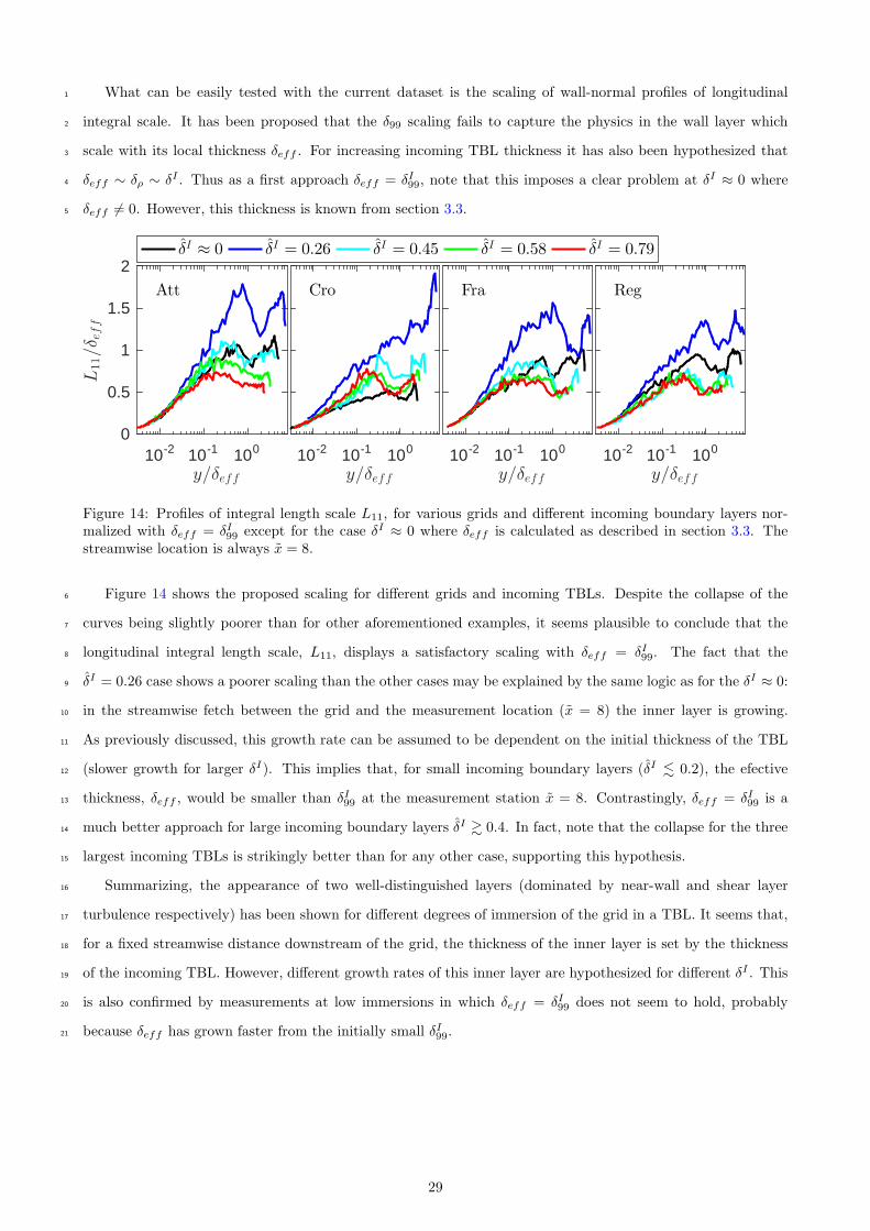
What can be easily tested with the current dataset is the scaling of wall-normal profiles of longitudinal1
integral scale. It has been proposed that the δ99 scaling fails to capture the physics in the wall layer which2
scale with its local thickness δeff . For increasing incoming TBL thickness it has also been hypothesized that3
δeff ∼ δρ ∼ δI . Thus as a first approach δeff = δI99, note that this imposes a clear problem at δI ≈ 0 where4
δeff 6= 0. However, this thickness is known from section 3.3.5
10-2 10-1 100
y/δeff
0
0.5
1
1.5
2
L11/δ e
ff
Att
δI ≈ 0 δI = 0.26 δI = 0.45 δI = 0.58 δI = 0.79
10-2 10-1 100
y/δeff
Cro
10-2 10-1 100
y/δeff
Fra
10-2 10-1 100
y/δeff
Reg
Figure 14: Profiles of integral length scale L11, for various grids and different incoming boundary layers nor-malized with δeff = δI99 except for the case δI ≈ 0 where δeff is calculated as described in section 3.3. Thestreamwise location is always x = 8.
Figure 14 shows the proposed scaling for different grids and incoming TBLs. Despite the collapse of the6
curves being slightly poorer than for other aforementioned examples, it seems plausible to conclude that the7
longitudinal integral length scale, L11, displays a satisfactory scaling with δeff = δI99. The fact that the8
δI = 0.26 case shows a poorer scaling than the other cases may be explained by the same logic as for the δI ≈ 0:9
in the streamwise fetch between the grid and the measurement location (x = 8) the inner layer is growing.10
As previously discussed, this growth rate can be assumed to be dependent on the initial thickness of the TBL11
(slower growth for larger δI). This implies that, for small incoming boundary layers (δI . 0.2), the efective12
thickness, δeff , would be smaller than δI99 at the measurement station x = 8. Contrastingly, δeff = δI99 is a13
much better approach for large incoming boundary layers δI & 0.4. In fact, note that the collapse for the three14
largest incoming TBLs is strikingly better than for any other case, supporting this hypothesis.15
Summarizing, the appearance of two well-distinguished layers (dominated by near-wall and shear layer16
turbulence respectively) has been shown for different degrees of immersion of the grid in a TBL. It seems that,17
for a fixed streamwise distance downstream of the grid, the thickness of the inner layer is set by the thickness18
of the incoming TBL. However, different growth rates of this inner layer are hypothesized for different δI . This19
is also confirmed by measurements at low immersions in which δeff = δI99 does not seem to hold, probably20
because δeff has grown faster from the initially small δI99.21
29

4 Conclusions1
A comprehensive flow characterization using one- and two-point hot-wire anemometry has been conducted2
downstream of single- and multi-scale wall-mounted highly porous fences. The bulk behaviour of the grids,3
studied by means of their drag, seems to be mainly dependent on their blockage ratio (which is kept the same4
for the various grids). However, slightly smaller value is detected for the Cro grid most likely due to the5
appearance of non-zero vertical velocity and the smaller aspect ratio of its bars. From another perspective,6
turbulent properties are shown to be dependent on the different distributions of blockage formed of bars of7
distinct sizes and orientations. These grids therefore generate a highly complex and inhomogeneous flow in8
their vicinity which interacts with the wall and evolves progressively towards a canonical turbulent boundary9
layer state. In this adaptation region, the turbulence of the bars’ wakes seems to decay much faster than that10
generated by either the wall or the shear layer appearing between the grid’s wake and the freestream. This is11
most likely due to the large mean shear appearing in these two regions which promotes turbulence production12
enhancing the fluctuations at these layers. Consequently the flow physics in the adaptation region are dominated13
by two different mechanisms depending on whether one considers the wall layer or the shear layer. In particular,14
spectra at large distances from the wall are shown to be clearly related with shear-layer thickness and, similarly,15
spectra in the near-wall region seem to follow the typical scaling of wall-bounded flows (λ+x ≈ 1000).16
The appearance of this clear separation of spectral behaviour along the wall-normal coordinate has enabled17
the definition a well-differentiated wall layer of effective thickness δeff . The thickness of this layer can also18
be established as a function of the point at which the wall normal profile of streamwise velocity correlation19
falls below a certain threshold (δρ). Both scalings can provide a measurement of the thickness of the wall layer20
although the latter seems to provide a more accurate description. The thickness of the wall layer is defined as21
the thickness of a naturally growing TBL which presents the same properties of that inner layer which develops22
under the influence of the fences’ wakes. Both δρ and δeff are shown to increase with x approaching δ99 or even23
exceeding it.24
Since this effective thickness can be understood as the upper boundary condition of the wall layer; δρ25
dominates the scaling of velocity fluctuations inside this region. In particular, a satisfactory scaling in terms of26
δρ is shown to hold for root-mean-square level of the wall shear stress fluctuations (τ ′+w,rms), longitudinal integral27
length scale (L11) and spanwise turbulent structure (ρuu(z)). Furthermore, details of the spanwise turbulent28
structure has also shown that large structures flanked by opposite sign fluctuations are not present for Att and29
Cro grids before 24h. For x > 24 and for the other two grids (every x) these large structures appear in the30
logarithmic layer with a separation of 0.3δρ (similar to a natural TBL).31
For cases where the incoming boundary layer was finite and comparable to the grid height h; the effective32
thickness of this inner layer is shown to scale with the thickness of the incoming TBL, δI ; at least for values of33
δI & 0.4. Furthermore, it is conjectured that the growth rate of δeff is also dependent on the incoming TBL34
thickness. In particular, it seems to grow faster for smaller δI .35
Despite the length of the adaptation region and the potential recovery of canonical TBL properties down-36
30
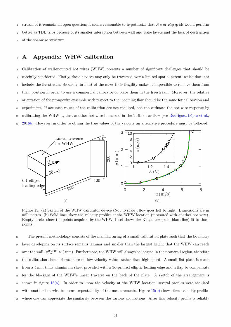
stream of it reamain an open question; it seems reasonable to hypothesize that Fra or Reg grids would perform1
better as TBL trips because of its smaller interaction between wall and wake layers and the lack of destruction2
of the spanwise structure.3
A Appendix: WHW calibration4
Calibration of wall-mounted hot wires (WHW) presents a number of significant challenges that should be5
carefully considered. Firstly, these devices may only be traversed over a limited spatial extent, which does not6
include the freestream. Secondly, in most of the cases their fragility makes it impossible to remove them from7
their position in order to use a commercial calibrator or place them in the freestream. Moreover, the relative8
orientation of the prong-wire ensemble with respect to the incoming flow should be the same for calibration and9
experiment. If accurate values of the calibration are not required, one can estimate the hot wire response by10
calibrating the WHW against another hot wire immersed in the TBL shear flow (see Rodrıguez-Lopez et al.,11
2016b). However, in order to obtain the true values of the velocity an alternative procedure must be followed.12
(a)
0 2 4 6 8u (m/s)
0
1
2
3
y(m
m)
1 1.2 1.4E (V)
0
2
4
6
8
10u(m
/s)
(b)
Figure 15: (a) Sketch of the WHW calibrator device (Not to scale), flow goes left to right. Dimensions are inmillimetres. (b) Solid lines show the velocity profiles at the WHW location (measured with another hot wire).Empty circles show the points acquired by the WHW. Inset shows the King’s law (solid black line) fit to thosepoints.
The present methodology consists of the manufacturing of a small calibration plate such that the boundary13
layer developing on its surface remains laminar and smaller than the largest height that the WHW can reach14
over the wall (yWHWmax ≈ 3mm). Furthermore, the WHW will always be located in the near-wall region, therefore15
the calibration should focus more on low velocity values rather than high speed. A small flat plate is made16
from a 4mm thick aluminium sheet provided with a 3d-printed elliptic leading edge and a flap to compensate17
for the blockage of the WHW’s linear traverse on the back of the plate. A sketch of the arrangement is18
shown in figure 15(a). In order to know the velocity at the WHW location, several profiles were acquired19
with another hot wire to ensure repeatability of the measurements. Figure 15(b) shows these velocity profiles20
where one can appreciate the similarity between the various acquisitions. After this velocity profile is reliably21
31

known, the calibration procedure consisted of sampling the WHW for 20 s at different wall-normal locations1
(from its minimum position yWHW0 = 0.18mm until 1.5mm in steps of 0.25mm and a further measurement at2
yWHW = 3mm). The WHW response at these locations is associated with the known velocity at the same y3
which is known from the velocity profiles acquisition. Once the response of the WHW is known, the coefficients4
A, B and C of the King’s law (E2 = A+BUC) are estimated by a least-squares fit.5
Figure 15(b) shows the values of the WHW response compared with the velocity profile measured before6
the calibration procedure. The agreement between these measurements and the velocity profiles is remarkably7
good at low velocities. However, it diverges slightly for the largest height, probably as a consequence of the8
interference of the prongs with the incoming fluid. Note that, at this position, the prong-to-prong distance is9
similar to its elevation over the wall hence some interaction may be expected. This is not expected to affect the10
results since this interference primarily affects the mean value and the current study only uses the fluctuations.11
The agreement with the King’s law is shown in the inset of figure 15(b) also displaying a remarkable agreement.12
B Appendix: Cd determination13
Let us consider a two-dimensional domain with its lower limit in the wall and the upper limit taken to be14
an undisrupted streamline far enough from the wall and the grid such that no mass or momentum cross this15
boundary. The subscripts 1 and 2 will denote the inlet (left) and outlet (right) of this domain respectively. We16
can write the mean integral momentum balance for this domain as:17
∫ y1
0
ρu21(y)dy +
∫ y1
0
p1(y)dy −∫ y2
0
ρu22(y)dy −
∫ y2
0
p2(y)dy = D +
∫ x2
x1
τw(x)dx . (5)
The selection of the region of the flow is not trivial and one should take some considerations prior to its18
determination. On the one hand taking x2 close to the grid (e.g. Dong et al., 2008) enables us to neglect the19
contribution of the shear stress term, which usually is difficult to measure or estimate. On the other hand, close20
to the grid the pressure contribution may be important and the spanwise inhomogeneities of the grid would21
make it impossible to assume two-dimensionality of the measurement domain. Seginer (1972) showed that the22
contribution of the term in p2 reduces drastically for x2 − x1 ≈ 10. Furthermore, the simplification of the 3D23
problem into a 2D domain can only be done after the spanwise inhomogeneities have dissappeared. Preliminary24
measurements (not shown for brevity) confirm that the spanwise homogeneity of the mean and rms profiles25
are significantly reduced for x > 5. The downstream limit of the domain should be therefore located further26
from that location. In order to find a compromise, the selected domain will have x1 upstream of the grid and27
x2 = 8h downstream of it. Moreover, since the upper edge of the domain is taken to be sufficiently far from the28
wall, we can assume that y2 ≈ y1 for simplicity although it does not have any effect on the results.29
With respect to the upstream limit of the domain, this will be taken to be x1 = −1, that is, at the leading30
edge of the flat plate. At this point the momentum thickness θ1 = 0 independently of the grid being mounted31
or not.32
32

For long streamwise domains (as the one considered), Seginer (1972) reported a low contribution of the1
pressure terms to the drag balance. Furthermore, under boundary layer assumptions, we could assume p(y) ≈ pw2
independent of y. Note in figure 1(a) that for x = 8 ↔ x = 0.9m, the wall pressure for the various grid cases is3
approximately the same as in the natural case. Therefore, we can assume that the flow is quasi-zero pressure4
gradient since variations in Cp are always smaller than 2%. Note that, strictly speaking p(y) ≈ pw may ot hold5
in the grids’ wake. However, preliminary measurements (not shown) reported a decrease of the wall-normal6
velocity for streamwise locations x > 2 which may support the use of this approximation. Hence it seems7
reasonable to neglect the contribution to the drag of the pressure difference across the domain.8
Under these assumptions, non-dimensionalizing the equations with the grid height h, and the freestream9
velocity U∞, and expressing the velocity profiles in terms of the momentum thickness θ =∫
∞
0[u(1 − u)]dy;10
equation (5) results:11
Cd ≈ 2
h
[
θ2 −1
ρU2∞
∫ x2
x1
τw(x)dx
]
. (6)
Where the wall shear stress term remains unknown because measurements of τw are not available for every12
x1 ≤ x ≤ x2. However, τw is known at station 2 (Rodrıguez-Lopez et al., 2017, and Table 2). In order to13
provide a meaningful estimation for the last term, let us consider the natural TBL case (without any grid14
installed), for this case we can write∫ x2
x1τNw dx ∝ θN2 , where superscript N denotes the natural case and, as15
mentioned above, θN1 = θ1 = 0. Given that we have the measurement of the wall shear stress at x2, we can use16
this information to approximate the last term in equation (6) as:17
1
ρU2∞
∫ x2
x1
τw(x)dx ≈ τGN 1
ρU2∞
∫ x2
x1
τNw (x)dx ≈ τGNθN2 , (7)
where τGN = τw(x2)/τNw (x2) is the relationship between the wall shear stress in the grid and the natural cases18
at x2. Note that the history of the wall shear stress between x1 and x2 is not known but we know the streamwise19
development of τw(x) for x > x2 as shown in Table 2. There, one can see that the shear stress remains relatively20
constant along x > x2 which sustains the use of τw(x2) as a control parameter for τw(x < x2). In any case,21
it has been shown (Table 3) that the contribution of the wall shear stress term to the drag determination is22
smaller than 10% hence variations in the modelization of this term have a rather limited impact in Cd.23
Thus the drag coefficient of the grids can be estimated as24
Cd ≈ 2
h
[
θ2 − θN2 τGN]
. (8)
References25
Alfredsson, P. H., Segalini, A., and Orlu, R. (2011). A new scaling for the streamwise turbulence intensity in26
wall-bounded turbulent flows and what it tells us about the ”outer” peak. Physics of Fluids, 23(4):041702.27
Andreopoulos, J. and Wood, D. H. (1982). The response of a turbulent boundary layer to a short length of28
surface roughness. Journal of Fluid Mechanics, 118:143–164.29
33

Antonia, R. A. and Luxton, R. E. (1971). The response of a turbulent boundary layer to a step change in1
surface roughness Part 1 . Smooth to rough. Journal of Fluid Mechanics, 48(4):721–761.2
Boppe, R. S., Neu, W. L., and Shuai, H. (1999). Large-scale motions in the marine atmospheric surface layer.3
Boundary-Layer Meteorology, 92(2):165–183.4
Brown, G. L. and Thomas, A. S. W. (1977). Large structure in a turbulent boundary layer. Physics of Fluids,5
20(10):243–252.6
Brunn, H. (1995). Hot-wire anemometry. UOP Oxford, Oxford, United Kingdom.7
Castro, I. (1971). Wake characteristics of two-dimensional perforated plates normal to an air-stream. Journal8
of Fluid Mechanics, 46(3):599–609.9
Chauhan, K. A., Monkewitz, P. A., and Nagib, H. M. (2009). Criteria for assessing experiments in zero pressure10
gradient boundary layers. Fluid Dynamics Research, 41(2):021404.11
Chernyshenko, S. I. and Baig, M. F. (2005a). Streaks and vortices in near-wall turbulence. Philosophical12
Transactions of the Royal Society, 363:1097–107.13
Chernyshenko, S. I. and Baig, M. F. (2005b). The mechanism of streak formation in near-wall turbulence.14
Journal of Fluid Mechanics, 544:99–131.15
Chew, Y. T., Khoo, B. C., Lim, C. P., and Teo, C. J. (1998). Dynamic response of hot-wire-anemometer. PartII:16
A flush-mounted hot-wire and hot-film probes for wall shear stress measurements. Measurement Science &17
Technology, 9(5):764–778.18
Counihan, J. (1969). An improved method of simulating an atmospheric boundary layer in a wind tunnel.19
Atmospheric Environment, 3(2):197–214.20
Dairay, T., Obligado, M., and Vassilicos, J. C. (2015). Non-equilibrium scaling laws in axisymmetric turbulent21
wakes. Journal of Fluid Mechanics, 781:166–195.22
Degraa, D. B., Webster, D. R., and Eaton, J. K. (1999). The effect of Reynolds number on boundary layer23
turbulence. Experimental Thermal and Fluid Science, 18:341–346.24
Del Alamo, J. C. and Jimenez, J. (2009). Estimation of turbulent convection velocities and corrections to25
Taylor’s approximation. Journal of Fluid Mechanics, 640:5–26.26
Dıaz-Daniel, C., Laizet, S., and Vassilicos, J. C. (2017). Wall shear stress fluctuations: mixed scaling and their27
effects on velocity fluctuations in a turbulent boundary layer. Physical Review Fluids, Under review.28
Dogan, E., Hanson, R. E., and Ganapathisubramani, B. (2016). Interactions of large-scale free-stream turbulence29
with turbulent boundary layers. Journal of Fluid Mechanics, 802:79–107.30
Dong, Z., Mu, Q., Luo, W., Qinan, G., Lu, P., and Wang, H. (2008). An analysis of drag force and moment for31
upright porous wind fences. Journal of Geophysical Research, 113(D4):1–8.32
Efros, V. and Krogstad, P.-A. (2011). Development of a turbulent boundary layer after a step from smooth to33
rough surface. Experiments in Fluids, 51(6):1563–1575.34
Erm, L. P. and Joubert, P. N. (1991). Low-Reynolds-number turbulent boundary layers. Journal of Fluid35
Mechanics, 230:1–44.36
Ganapathisubramani, B., Hutchins, N., Hambleton, W. T., Longmire, E. K., and Marusic, I. (2005). Investi-37
34

gation of large-scale coherence in a turbulent boundary layer using two-point correlations. Journal of Fluid1
Mechanics, 524(2005):57–80.2
Geng, C., He, G., Wang, Y., Xu, C., Lozano-Duran, A., and Wallace, J. M. (2015). Taylor’s hypothesis in3
turbulent channel flow considered using a transport equation analysis. Physics of Fluids, 27(2):025111.4
Goh, K., Geipel, P., and Lindstedt, R. (2014). Lean premixed opposed jet flames in fractal grid generated5
multiscale turbulence. Combustion and Flame, 161(9):2419–2434.6
Goh, K. H. H., Geipel, P., Hampp, F., and Lindstedt, R. P. (2013). Flames in fractal grid generated turbulence.7
Fluid Dynamics Research, 45(6):061403.8
Gomes-Fernandes, R., Ganapathisubramani, B., and Vassilicos, J. C. (2012). Particle image velocimetry study9
of fractal-generated turbulence. Journal of Fluid Mechanics, 711:306–336.10
Good, M. and Joubert, P. N. (1968). The form drag of two-dimensional bluff-plates immersed in turbulent11
boundary layers. Journal of Fluid Mechanics, 31(3):547–582.12
Groth, J. and Johansson, A. V. (1988). Turbulence reduction by screens. Journal of Fluid Mechanics, 197:139–13
155.14
Guan, D., Zhang, Y., and Zhu, T. (2003). A wind-tunnel study of windbreak drag. Agricultural and Forest15
Meteorology, 118(1-2):75–84.16
Hanson, R. E. and Ganapathisubramani, B. (2016). Development of turbulent boundary layers past a step17
change in wall roughness. Journal of Fluid Mechanics, 795:494–523.18
Hoerner, S. F. (1965). Fluid-dynamic drag: practical information on aerodynamic drag and hydrodynamic19
resistance. Hoerner Fluid Dynamics, 2nd edition.20
Hultmark, M., Ashok, A., and Smits, A. J. (2011). A new criterion for end-conduction effects in hot-wire21
anemometry. Measurement Science and Technology, 22(5):055401.22
Hunt, J. C. R. and Fernholz, H. (1975). Wind-tunnel simulation of the atmospheric boundary layer: a report23
on Euromech 50. Journal of Fluid Mechanics, 70(3):543–559.24
Hurst, D. and Vassilicos, J. C. (2007). Scalings and decay of fractal-generated turbulence. Physics of Fluids,25
19(3):035103.26
Hutchins, N. and Marusic, I. (2007a). Evidence of very long meandering features in the logarithmic region of27
turbulent boundary layers. Journal of Fluid Mechanics, 579:1–28.28
Hutchins, N. and Marusic, I. (2007b). Large-scale influences in near-wall turbulence. Philosophical transactions.29
Series A, Mathematical, physical, and engineering sciences, 365(1852):647–64.30
Hutchins, N., Nickels, T. B., Marusic, I., and Chong, M. S. (2009). Hot-wire spatial resolution issues in wall-31
bounded turbulence. Journal of Fluid Mechanics, 635:103–136.32
Jimenez, J. (2004). Turbulent Flows Over Rough Walls. Annual Review of Fluid Mechanics, 36(1):173–196.33
Keylock, C. J., Nishimura, K., Nemoto, M., and Ito, Y. (2012). The flow structure in the wake of a fractal fence34
and the absence of an inertial regime. Environmental Fluid Mechanics, 12(3):227–250.35
Li, B. and Sherman, D. J. (2015). Aerodynamics and morphodynamics of sand fences: A review. Aeolian36
Research, 17:33–48.37
35

Marusic, I. and Heuer, W. D. C. (2007). Reynolds number invariance of the structure inclination angle in wall1
turbulence. Physical Review Letters, 99(11):114504.2
Marusic, I. and Kunkel, G. J. (2003). Streamwise turbulence intensity formulation for flat-plate boundary layers.3
Physics of Fluids, 15(8):2461–2464.4
Marusic, I., McKeon, B. J., Monkewitz, P. A., Nagib, H. M., Smits, A. J., and Sreenivasan, K. R. (2010).5
Wall-bounded turbulent flows at high Reynolds numbers: Recent advances and key issues. Physics of Fluids,6
22(6):065103.7
Mathis, R., Hutchins, N., and Marusic, I. (2011). A predictive inner-outer model for streamwise turbulence8
statistics in wall-bounded flows. Journal of Fluid Mechanics, 681:537–566.9
Mathis, R., Marusic, I., Chernyshenko, S. I., and Hutchins, N. (2013). Estimating wall-shear-stress fluctuations10
given an outer region input. Journal of Fluid Mechanics, 715:163–180.11
Mazellier, N. and Vassilicos, J. C. (2010). Turbulence without Richardson-Kolmogorov cascade. Phys. Fluids,12
22(7):075101.13
Melina, G., Bruce, P. J. K., and Vassilicos, J. C. (2016). Vortex shedding effects in grid-generated turbulence.14
Physical Review Fluids, 1(4):044402.15
Miller, M., Estejab, B., and Bailey, S. C. C. (2014). Evaluation of hot-wire spatial filtering corrections for wall16
turbulence and correction for end-conduction effects. Experiments in Fluids, 55(5):1735.17
Nedic, J., Ganapathisubramani, B., Vassilicos, J. C., Boree, J., Brizzi, L. E., and Spohn, A. (2012). Aeroacoustic18
Performance of Fractal Spoilers. AIAA Journal, 50(12):2695–2710.19
Nedic, J. and Vassilicos, J. C. (2015). Vortex shedding and aerodynamic performance of an airfoil with multi-20
scale trailing edge modifications. AIAA Journal, 53(11):1–24.21
Orlu, R. and Schlatter, P. (2013). Comparison of experiments and simulations for zero pressure gradient22
turbulent boundary layers at moderate Reynolds numbers. Experiments in Fluids, 54(6):1547.23
Ranga-Raju, K. G., Garde, R. J., Singh, S. K., and Sing, N. (1988). Experimental study on characteristics of24
flow past porous fences. Journal of Wind Engineering and Industrial Aerodynamics, 29(1-3):155–163.25
Robinson, S. K. (1986). Instantaneous velocity profile measurements in a turbulent boundary layer. Chemical26
Engineering Communications, 43(4):347–369.27
Rodrıguez-Lopez, E., Bruce, P. J. K., and Buxton, O. R. H. (2015). A robust post-processing method to28
determine skin friction in turbulent boundary layers from the velocity profile. Experiments in Fluids, 56(4):68.29
Rodrıguez-Lopez, E., Bruce, P. J. K., and Buxton, O. R. H. (2016a). Near field development of artificially30
generated high Reynolds number turbulent boundary layers. Physical Review Fluids, 1(7):074401.31
Rodrıguez-Lopez, E., Bruce, P. J. K., and Buxton, O. R. H. (2016b). On the formation mechanisms of artificially32
generated high reynolds number turbulent boundary layers. Boundary-Layer Meteorology, 160(2):201–224.33
Rodrıguez-Lopez, E., Bruce, P. J. K., and Buxton, O. R. H. (2017). Experimental measurement of wall shear34
stress in strongly disrupted flows. Journal of Turbulence, 18(3):271–290.35
Schlatter, P. and Orlu, R. (2010). Assessment of direct numerical simulation data of turbulent boundary layers.36
Journal of Fluid Mechanics, 659:116–126.37
36

Schlatter, P. and Orlu, R. (2012). Turbulent boundary layers at moderate Reynolds numbers: inflow length1
and tripping effects. Journal of Fluid Mechanics, 710:5–34.2
Seginer, I. (1972). Windbreak drag calculated from the horizontal velocity field. Boundary-Layer Meteorology,3
3(1):87–97.4
Sillero, J. A., Jimenez, J., and Moser, R. D. (2013). One-point statistics for turbulent wall-bounded flows at5
Reynolds numbers up to δ{\approx}2000. Physics of Fluids, 25(10):105102.6
Steiros, K., Bruce, P. J. K., Buxton, O. R. H., and Vassilicos, J. C. (2017). Power consumption and form drag7
of regular and fractal-shaped turbines in a stirred tank. AIChE Journal, 63(2):843–854.8
Taylor, G. (1963). The Scientific Papers of G. I. Taylor. Vol. III. Aerodynamics and the Mechanics of Projectiles9
and Explosions. Cambridge University Press, Cambridge.10
Townsend, A. (1976). The Structure of Turbulent Shear Flow. Cambridge university Press, Cambridge and New11
York, 2 edition.12
Valente, P. C. and Vassilicos, J. C. (2014). The non-equilibrium region of grid-generated decaying turbulence.13
Journal of Fluid Mechanics, 744:8–37.14
Wilson, J. D. (1987). On the choice of a windbreak porosity profile. Boundary-Layer Meteorology, 38(1):37–49.15
Woodruff, N. P., Fryrear, D. W., and Lyles, L. (1963). Engineering similitude and momentum transfer principles16
applied to shelterbelt studies. Transactions of the ASME, 6(1):41–47.17
37