Fluid dynamics and mixing behavior of a static mixer using ...ltces.dem.ist.utl.pt/lxlaser/lxlaser2008/papers/01.2_3.pdf · 14th Int Symp on Applications of Laser Techniques to Fluid

14th Int Symp on Applications of Laser Techniques to Fluid Mechanics Lisbon, Portugal, 07-10 July, 2008

- 1 -

Fluid dynamics and mixing behavior of a static mixer using simultaneously

Particle Image Velocimetry and Planar Laser-Induced Fluorescence measurements

Andreas Lehwald1, Stefan Leschka

1,2, Katharina Zähringer

3, Dominique

Thévenin4

1: Lab. of Fluid Dynamics and Technical Flows, Otto-von-Guericke-University, Magdeburg, Germany,

[email protected]

2: now at Hydraulic & Coastal Engineering, DHI-WASY GmbH, Syke, Germany,

[email protected]


[email protected]


[email protected]

Abstract The mixing behavior around a SMX-type static mixer segment has been investigated experimentally by using Particle Image Velocimetry (PIV) and Planar Laser-Induced Fluorescence (PLIF) simultaneously. To quantify mixing, velocity fields and concentration fields have been measured for different Reynolds numbers along vertical and horizontal sections directly behind the mixer. The experimental data have been post-processed. A spectral analysis of the simultaneous PIV and PLIF measurements has been carried out, in order to determine the characteristic frequencies induced by the mixer and correlations between velocity and concentrations. Furthermore, the mixing efficiency has been quantified by considering the segregation index.

Introduction

In the past, the mixing behavior of static mixers has been investigated in a global manner for

various mixer configurations, but usually without relying on non-intrusive optical diagnostics. For

example Pahl and Muschelknautz (1982) have compared 12 different static mixer types, but

considering only global properties, like pressure drop and overall mixing efficiency.

Recently, static mixers have been also characterized using Planar Laser-Induced Fluorescence

(PLIF) to determine the concentration fields and the concentration variance, a characteristic

parameter to quantify macro-mixing. A few generic configurations (Wadley and Dawson, 2005) and

commercial static mixers (Pust et al., 2006) have been investigated in this manner. This is an

essential step, but an isolated PLIF measurement cannot deliver information concerning the flow

structure.

In the present project Particle Image Velocimetry (PIV) and PLIF have been combined and used

simultaneously to quantify experimentally the fluid behavior around a static mixer, in particular to

determine the flow and mixing conditions behind an isolated mixer segment. The considered

configuration is a SMX-type static mixer (fig. 1). These extensive experimental measurements are

additionally employed to check and improve numerical mixing models and to validate

computational simulations relying on Large-Eddy Simulations (LES). Such LES computations

should ultimately be able to characterize in an accurate manner the properties of industrial static

mixers.


- 2 -

Experimental set-up and measurement methods

In order to obtain laminar conditions at the inlet of the mixer, a gravity-driven flow channel

installation is used (fig. 2). For that, a pump delivers the fluid from a lower tank to an upper tank,

whose water level lies roughly 10 m above the channel axis. A diffuser is installed, which is used

after the down-pipe to adapt the cross-section from circular to square. This square shape has been

chosen for the whole measurement section in order to increase the quality of all optical

measurements by limiting refraction, laser beam divergence and image distortion. After the diffuser,

a 2.45 m long inflow section leads the fluid to the static mixer. The mixer consists of seven

rectangular lamellas with an individual width of 13 mm, as illustrated in figure 1. Four lamellas are

turned against the flow; between them, three are turned in the direction of the flow. The straight

outflow section behind the mixer also has a length of 2.45 m. Inflow, outflow and mixer consist of

acrylic glass and have a cross section of 91 x 91 mm². A flow meter is installed at the end of the test

section. The required flow-rates are adjusted using a precision control valve. From there, the fluid

goes to a damper. For simultaneous PIV and PLIF measurements, the water contains not only PIV

tracers but also the fluorescence dye. It is sent to a purification process, so that the dye does not re-

circulate in the installation (open loop). A schematic view of the experimental set-up developed for

the present investigation is shown in figure 2. Further details can be found in Leschka et al. (2006).

Figure 1. SMX-type static mixer considered in this study,

a) top view: horizontal (x-y) plane, b) side view: vertical (x-z) plane.

Figure 2. Schematic view of the experimental set-up.

For PIV measurements tracer particles are injected into the upper tank (fig. 2). Spherical hollow

glass balls (Type 110 P8 CP00) with a mean diameter of d50 = 10.2 µm (d10 = 2.9 µm, d90 = 21.6

µm), a mean density of 1.1 g/cm³ and a bulk volume between 2.22 l/kg and 2.85 l/kg have been

used. Depending on the fluid velocities, the tracer concentration is adapted to obtain 30 to 40

particles in a 32 x 32 pixel interrogation area of the PIV image. This results in a typical volume


- 3 -

fraction of Vp/Vf = 6.86·10-5

, low enough to avoid any influence of the particles on the flow.

For mixing measurements using PLIF, the fluorescence tracer (99% pure Rhodamine 6G) is

injected along the centerline, 39 mm in front of the mixer segment, with the same velocity as the

main fluid and with a Rhodamine concentration of 20 µg/l. The PLIF images have been acquired

using an intensified CCD camera (LaVision NanoStar, 1280 x 1024 pixels) during the first of two

PIV laser pulses (Nd:YAG, 532 nm, 80 mJ per pulse), while the CCD camera (LaVision Imager

Intense, 1600 x 1186 pixels) used for PIV takes double images, used to calculate the two-

dimensional velocity fields. To separate PIV and PLIF signals, the cameras are equipped with two

different filters. For recording PIV images a laser-line filter BP532/10 nm and for recording PLIF

images a high-pass filter LP580 nm have been used, respectively.

The outlet of the central LIF tracer injection system has a square section of 25 mm². Before entering

the test-section, the injected mixture of water and fluorescing dye flows through a thermostat

(Haake Phoenix 2 P1-C25P), which is used to control the temperature of the injected fluid and keep

the difference with the main fluid temperature within the channel below 0.5 K. The temperatures

typically lie around 17 °C in all experiments presented here. This very accurate temperature control

was observed to be absolutely necessary, in order to avoid a rapid stratification between the injected

mixture and the main flow, due to buoyancy.

The static over-pressure in the test-section is 0.872 bar. The Reynolds numbers are always

calculated using the hydraulic diameter of the channel and the mean streamwise velocities.

The resulting values of the Reynolds number Re together with the corresponding total flow rate and

the flow rates Q1 of main fluid and Q2 of the injected mixture, their ratio and the mean streamwise

velocities are summarized in table 1 for the two main cases (Re = 562 and Re = 1000) discussed in

this paper.

Static mixers are usually employed for highly viscous fluids and thus very low Reynolds numbers.

The present experiments use water as a main fluid but keep the analogy by considering the same

typical Reynolds numbers (similarity conditions), thus leading to very low velocities.

Table 1. Reynolds numbers, flow rates and resulting mean axial velocities.

Re [-] Q [l/h] Q1 [l/h] Q2 [l/h] ux

[mm/s] +

2

1 2

Q

Q Q [-]

562 184.8 184.0 0.826 6.2 4.5·10-3

1000 328.9 327.2 1.714 11.0 5.2·10-3

The PIV data has been post-processed and evaluated using an adaptive multi pass cross-correlation

with decreasing size over interrogation areas of 128 x 128, 64 x 64 and 32 x 32 pixels, each with 50

% overlapping. Furthermore, a Gaussian low-pass filter has been applied. In the interrogation area,

values lying within the range of 120 % of the second highest value have been accepted.

For PLIF a concentration calibration is necessary. In the literature different specifications can be

found concerning the linear part of the fluorescence behavior of the employed dye. Therefore

several tests have been conducted in order to find an appropriate range for the present optical and

flow conditions. As recommended by Law and Wang (2000), a concentration range of 0 µg/l to 20

µg/l has been finally found to be suitable for these experiments. The Nd:YAG-laser has been

systematically combined with an energy monitor, which allows to correct laser energy fluctuations

during post-processing. This correction is necessary to obtain accurate quantitative concentrations

from PLIF. Post-processing masks have been defined to exclude non-evaluable areas due to locally

insufficiently good optical conditions, resulting from the lamellas, shadows of mounting screws,

etc. (see also fig. 1). In addition, background images have been acquired. In this manner negative

effects like background scattering (reflection, diffraction and refraction) can be eliminated.


- 4 -

Results

The results presented in figure 3 exemplify instantaneous simultaneous measurements involving

PIV and PLIF directly behind the mixer (x = 50) mm, in the central horizontal and vertical plane at

Re = 562 and Re = 1000. White zones in the images correspond to masked areas, in which

measurements are not possible.

Reynolds number 562 is the reference case for this study. Averaging the velocity measurements

over 300 images, velocity ranges of 0.3 mm/s up to 33 mm/s in the horizontal plane and of 0.4

mm/s to 22 mm/s in the vertical plane are obtained. The maximum velocity is measured, as

expected, in-between the mixer lamellas (lowest hydraulic section).

At Re = 1000 the flow shows more vertical structures and the velocity magnitudes range between

0.2 mm/s and 57 mm/s in the horizontal plane and between 0.3 mm/s and 42 mm/s in the vertical

plane.

The differences observed between horizontal and vertical measurements are not surprising, since

the single-stage mixer structure is not at all isotropic (fig. 1), with all lamellas positioned in the

vertical direction. For such low Reynolds numbers, the influence of the mixer geometry is expected

to be very high, leading to different results in the horizontal and vertical plane. This difference will

decrease when increasing the Reynolds number or when considering realistic mixer geometry with

several stages, turned one to the other at 90°, and thus increasing flow isotropy.

The concentration measurements clearly show at Re = 562 small-scale, coherent vortex structures

both in the horizontal and in the vertical plane. The measurements for the higher Reynolds number

do not present such clear vortex structures any more. Due to the small quantity of dye injected in

the main flow and to the higher dynamics of the flow a large part of the injected fluid is already

well-mixed when the fluid leaves the mixer segment. Qualitatively, a high level of mixing is, in

particular seen in the horizontal plane just behind the mixer, since the influence of the lamellas is

maximal in this plane. In the vertical plane, elongated vortex filaments are observed. As a whole,

mixing homogeneity increases with the Reynolds number, as expected. This will be quantified in

what follows.

Behind the mixer the flow velocities and concentrations have been analyzed extensively using Non-

equidistant Fast-Fourier Transformation (NFFT) in order to identify the characteristic frequencies f

of the structures induced by the static mixer both in the velocity and in the concentration fields.

During the simultaneous PIV/PLIF measurements, the obtained acquisition frequency is limited to

1.6 Hz at most and is furthermore not constant, due to the limited and different data transfer-rates of

the cameras. As a consequence, a classical FFT analysis is not possible any more. For the present

post-processing the efficient Lomb-Scargle-Algorithm (NFFT, cf. Press et al., 1995) has been used.

The frequency analysis of the PIV data delivers clear peaks and harmonics for Re = 562 and Re =

1000 in the horizontal as well as in the vertical planes (fig. 4). The PLIF frequency analysis shows a

lower signal-to-noise ratio in the horizontal plane, especially for Re = 1000. For Re = 562 the peak

frequencies for velocity magnitude, velocity direction and concentration are all equal to 0.36 Hz.

This means that the structures induced by the mixer repeat very clearly after 2.78 s, as can also be

shown by looking directly at time-sequences. For Re = 1000, a peak frequency of 0.75 Hz (period

of 1.33 s) has been found. For both planes and both values of Re the variations of the velocity field

correlate very well with the fluctuations of the concentration field.


- 5 -

PIV measurement: velocity vector field PLIF measurement: concentration field

Re

= 5

62

ho

rizo

nta

l p

lan

e

ver

tica

l p

lan

e

Re

= 1

00

0

ho

rizo

nta

l p

lan

e

ver

tica

l p

lan

e

Figure 3. Velocity vector fields (left) and concentration fields (right) measured directly behind the static mixer at

Reynolds number 562 (top) and 1000 (bottom) for the central horizontal and vertical planes.


- 6 -

NFFT of velocity magnitude NFFT of velocity direction NFFT of concentration

Re

= 5

62 h

ori

zon

tal

pla

ne

ver

tica

l p

lan

e

Re

= 1

00

0 h

ori

zon

tal

pla

ne

ver

tica

l p

lan

e

Figure 4. NFFT for velocity vector fields considering separately vector magnitude (left) and vector direction (middle),

as well as NFFT of concentration fields (right). All measurements have been carried out directly behind the mixer at

Reynolds number 562 (top) and 1000 (bottom) for horizontal and vertical planes.

For the quantification of the mixing efficiency the classical segregation index 2

2S

max

Iσ

σ= , given by

Danckwerts (1952) and based on the normalized concentration variance, has been calculated along

the channel axis. The variance of the concentration c(x) of the injected dye is calculated by

[ ]22 1

A

c( x ) µ dAA

σ = − ⋅∫ , with the expectation (mean) value 1

A

µ c( x ) dAA

= ⋅∫ . The maximum computed

variance 2

maxσ , used as a reference value for normalization, is computed by considering

independently all individual results (global maximum). For this treatment the measurement area has

been divided in regular stripes along the streamwise direction. In each stripe, the “local”, mean

concentration value and variance can be determined. After having determined the global maximum

of the variance, a segregation index can be calculated as a function of the streamwise coordinate for

each instantaneous PLIF image. The resulting segregation indices have then been averaged over 300


- 7 -

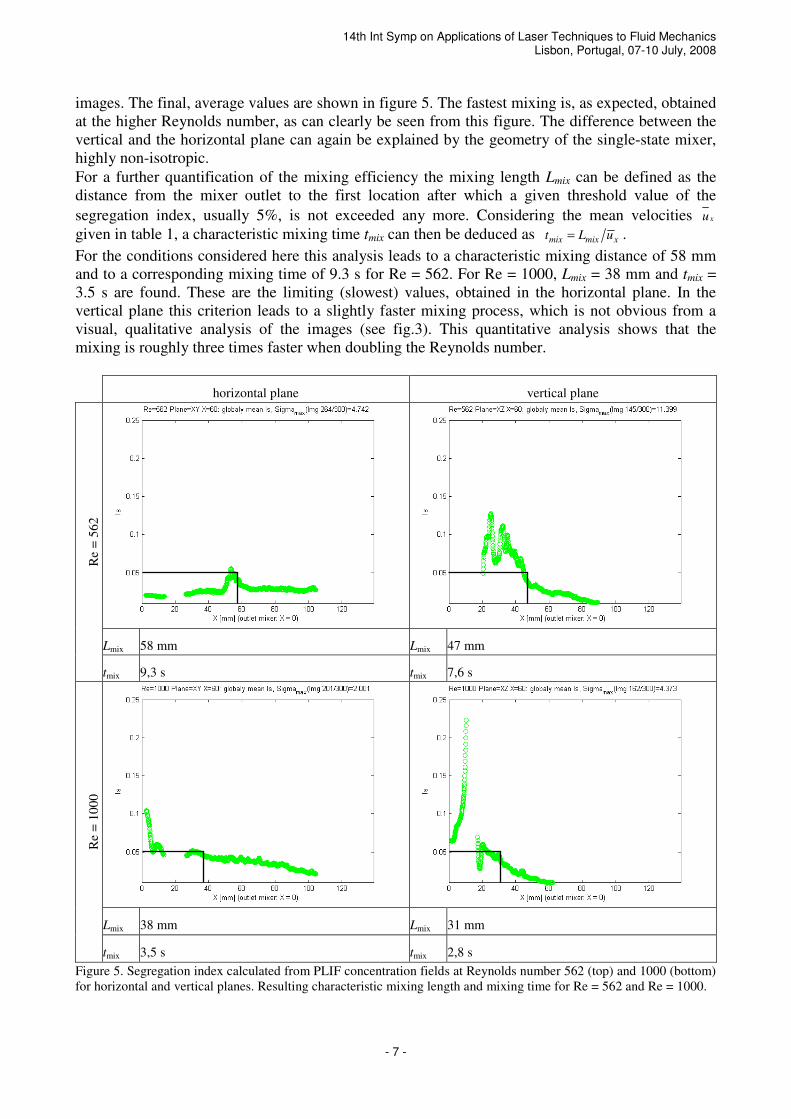
images. The final, average values are shown in figure 5. The fastest mixing is, as expected, obtained

at the higher Reynolds number, as can clearly be seen from this figure. The difference between the

vertical and the horizontal plane can again be explained by the geometry of the single-state mixer,

highly non-isotropic.

For a further quantification of the mixing efficiency the mixing length Lmix can be defined as the

distance from the mixer outlet to the first location after which a given threshold value of the

segregation index, usually 5%, is not exceeded any more. Considering the mean velocities xu

given in table 1, a characteristic mixing time tmix can then be deduced as xmixmix uLt = .

For the conditions considered here this analysis leads to a characteristic mixing distance of 58 mm

and to a corresponding mixing time of 9.3 s for Re = 562. For Re = 1000, Lmix = 38 mm and tmix =

3.5 s are found. These are the limiting (slowest) values, obtained in the horizontal plane. In the

vertical plane this criterion leads to a slightly faster mixing process, which is not obvious from a

visual, qualitative analysis of the images (see fig.3). This quantitative analysis shows that the

mixing is roughly three times faster when doubling the Reynolds number.

horizontal plane vertical plane

Re

= 5

62

Lmix 58 mm Lmix 47 mm

tmix 9,3 s tmix 7,6 s

Re

= 1

00

0

Lmix 38 mm Lmix 31 mm

tmix 3,5 s tmix 2,8 s

Figure 5. Segregation index calculated from PLIF concentration fields at Reynolds number 562 (top) and 1000 (bottom)

for horizontal and vertical planes. Resulting characteristic mixing length and mixing time for Re = 562 and Re = 1000.


- 8 -

Conclusions and present work

Thanks to such simultaneous PIV/PLIF measurements it is possible to characterize quantitatively

and in a non-intrusive manner the flow and mixing conditions behind static mixers, in particular to

determine characteristic flow frequencies, correlations between velocity and concentration fields

and to quantify mixing efficiency. In the near future similar simultaneous PIV and PLIF

measurements will be realized for up to four consecutive mixer segments, each of them turned by

π/2 compared to the previous one.

At present, mixing chemically reacting species in a liquid-liquid system is being characterized

experimentally, in order to quantify simultaneously micro-mixing and macro-mixing. For that

purpose, a preliminary study has demonstrated that fluorescein disodium salt (Uranine) can be used.

This fluorescence dye changes its fluorescence emission depending on the local pH-value, which

can be used to track micro-mixing. Figure 6 shows the fluorescence emission I as a function of the

pH-value for a range of the pH between 3.5 and 8.

relativ intensity [counts] = f(pH-value)

0,0

0,1

0,2

0,3

0,4

0,5

0,6

0,7

0,8

0,9

1,0

3,0 3,5 4,0 4,5 5,0 5,5 6,0 6,5 7,0 7,5 8,0 8,5pH-value [-]

I /

I ma

x [

-]

Figure 6. Fluorescence emission of fluorescein disodium salt (Uranine) as a function of the pH-value.

In this study hydrochloride acid (HCl) mixed with fluorescein disodium salt is injected into the

main fluid, which is an alkaline fluorescein disodium salt solution. The resulting acid-base reaction

changes the local pH-value and as a consequence the fluorescence properties of the fluorescein

disodium salt. Using equal concentrations of fluorescein disodium salt in both liquids, this local pH

modification can be quantified by PLIF and is a direct marker of the chemical reaction. PIV is again

employed simultaneously to analyze the velocity field.

All these experimental measurements will be made freely available to the scientific community

through a data-base accessible via Internet, which is already partly available under http://www.uni-

magdeburg.de/isut/LSS/Forschung/MASDOM/index.html.


- 9 -

Acknowledgments

The authors would like to acknowledge the financial support of the German Research Foundation

(DFG) through the Priority Programme “Analyse, Modellbildung und Berechnungen von

Strömungsmischern mit und ohne chemische Reaktion” (SPP1141). Interesting discussions with H.

Nobach (Max Planck Institute for Dynamics und Self-Organization, Goettingen, Germany)

concerning the frequency analysis of non-equidistant time-signals are gratefully acknowledged.

References

Danckwerths PV (1952) The definition and measurement of some characteristics of mixtures. Appl

Sci Res A3:279-296

Leschka S, Thévenin D, Zähringer K (2006) Fluid velocity measurements around a static mixer

usng Laser-Doppler Anemometry and Particle Image Velocimetry. Proceedings of the

Conference on Modelling Fluid Flow (Eds Lajos T, Vad J) Vol. 1, pp 639-646, Budapest,

ISBN 963 06 0361 6.

Law AWK, Wang H (2000) Measurement of mixing process with combined digital particle image

velocimetry and planar laser induced fluorescence. Exp Therm Fluid Sci 22:213-229

Leschka S, Thévenin D, Zähringer K (2006) Flow and mixing characterization of a static mixer

using Laser-Doppler Anemometry and simultaneous Particle-Image Velocimetry/Planar Laser-

Induced Fluorescence. NAMF Mixing XXI Conference, Park City, UT, 2007

Pahl MH, Muschelknautz E (1982) Static mixers and their applications. Int Chem Eng 22:197-205

Press W, Teukolsky S, Vetterling W, Flannery B (1995) Numerical Recipes in FORTRAN.

Cambridge University Press, ISBN 0 521 43064 X

Pust O, Strand T, Mathys P, Rütti A (2006) Quantification of Laminar Mixing Performance using

Laser-Induced Fluorescence. 13th International Symposium on Applications of Laser

Techniques to Fluid Mechanics, Lisbon 2006

Wadley R, Dawson MK (2005) LIF measurements of blending in static mixers in the turbulent and

transitional flow regimes. Chem Eng Sci 60 2469-2478

Documents

Fluid dynamics and mixing behavior of a static mixer using ...ltces.dem.ist.utl.pt/lxlaser/lxlaser2008/papers/01.2_3.pdf · 14th Int Symp on Applications of Laser Techniques to Fluid