Embed Size (px)
Citation preview
Heat Transfer
Thomas Rodgers
2013

Contents
List of Figures iii
1 Introduction to Heat Transfer 11.1 Introduction . . . . . . . . . . . . . . . . . . . . . . . . . . . . . . . . . 31.2 Forms of energy . . . . . . . . . . . . . . . . . . . . . . . . . . . . . . . 3
1.2.1 Heat . . . . . . . . . . . . . . . . . . . . . . . . . . . . . . . . . 41.2.2 Enthalpy . . . . . . . . . . . . . . . . . . . . . . . . . . . . . . 4
1.3 Specific heat capacity . . . . . . . . . . . . . . . . . . . . . . . . . . . . 51.4 Rate of Energy Uptake . . . . . . . . . . . . . . . . . . . . . . . . . . . 61.5 Latent heat of vaporisation/condensation (hfg) and latent heat of fusion/melt-
ing (hsf ) . . . . . . . . . . . . . . . . . . . . . . . . . . . . . . . . . . . 61.6 Thermophysical Properties of Water, Steam, and Air . . . . . . . . . . . 71.7 Conservation of energy and energy balances . . . . . . . . . . . . . . . . 9
1.7.1 Energy balances . . . . . . . . . . . . . . . . . . . . . . . . . . 91.7.2 Statement of the Law of Conservation . . . . . . . . . . . . . . . 101.7.3 Temperature-Enthalpy Diagrams . . . . . . . . . . . . . . . . . . 11
2 General Heat Transfer Equation 132.1 Introduction . . . . . . . . . . . . . . . . . . . . . . . . . . . . . . . . . 152.2 General Heat Transfer Equation . . . . . . . . . . . . . . . . . . . . . . 152.3 Mechanisms of Heat Transfer . . . . . . . . . . . . . . . . . . . . . . . . 16
2.3.1 Conduction . . . . . . . . . . . . . . . . . . . . . . . . . . . . . 162.3.2 Convection . . . . . . . . . . . . . . . . . . . . . . . . . . . . . 182.3.3 Radiation . . . . . . . . . . . . . . . . . . . . . . . . . . . . . . 22
2.4 The Standard Engineering Equation, and Analogy with Electrical Circuits 252.5 Problems . . . . . . . . . . . . . . . . . . . . . . . . . . . . . . . . . . 29
3 Heat Transfer by Conduction 313.1 Introduction . . . . . . . . . . . . . . . . . . . . . . . . . . . . . . . . . 333.2 Derivation of one-dimensional conduction heat transfer equation . . . . . 33
3.2.1 Rectangular Coordinates . . . . . . . . . . . . . . . . . . . . . . 363.2.2 Cylindrical Coordinates . . . . . . . . . . . . . . . . . . . . . . 363.2.3 Spherical Coordinates . . . . . . . . . . . . . . . . . . . . . . . 363.2.4 Special Cases . . . . . . . . . . . . . . . . . . . . . . . . . . . . 363.2.5 Physical Meaning of the Laplace Equation . . . . . . . . . . . . 38
3.3 Steady State Heat Conduction across a Slab . . . . . . . . . . . . . . . . 403.4 Steady State Heat Generation in a Slab Insulated on One Side . . . . . . . 42
i

CONTENTS
3.5 Temperature Profiles across Cylindrical Walls . . . . . . . . . . . . . . . 443.6 Temperature Profiles Across Spherical Walls . . . . . . . . . . . . . . . . 473.7 Boundary Conditions . . . . . . . . . . . . . . . . . . . . . . . . . . . . 48
3.7.1 Prescribed Temperature Boundary Condition (First Kind) . . . . . 483.7.2 Prescribed Heat Flux Boundary Condition (Second Kind) . . . . . 483.7.3 Convection Boundary Condition (Third Kind) . . . . . . . . . . . 49
3.8 Problems . . . . . . . . . . . . . . . . . . . . . . . . . . . . . . . . . . 51
4 Heat Transfer by Convection 534.1 Introduction . . . . . . . . . . . . . . . . . . . . . . . . . . . . . . . . . 554.2 Thermal Boundary Layer . . . . . . . . . . . . . . . . . . . . . . . . . . 554.3 Relating Convection Heat Transfer to Fluid Mechanics using Dimension-
less Numbers . . . . . . . . . . . . . . . . . . . . . . . . . . . . . . . . 564.4 Laminar Flow along a Flat Plate . . . . . . . . . . . . . . . . . . . . . . 574.5 Correlations for Predicting the Convection Heat Transfer Coefficient . . . 58
4.5.1 Forced Convection, Fully Developed Turbulent Flow in Smooth,Circular Pipes . . . . . . . . . . . . . . . . . . . . . . . . . . . . 58
4.5.2 Forced Convection, Laminar Flow over a flat Plate . . . . . . . . 604.5.3 Forced Convection, Turbulent Flow over a Flat Plate . . . . . . . 614.5.4 Forced Convection, Fully Developed Laminar Flow in Smooth,
circular Pipes . . . . . . . . . . . . . . . . . . . . . . . . . . . . 614.5.5 Forced Convection, Entrance Region of a Circular Tube . . . . . 614.5.6 Forced Convection, Fully Developed Turbulent Flow in Smooth,
Circular Pipes . . . . . . . . . . . . . . . . . . . . . . . . . . . . 614.6 Problems . . . . . . . . . . . . . . . . . . . . . . . . . . . . . . . . . . 63
5 Applications of Heat Transfer in Chemical Engineering 655.1 Introduction . . . . . . . . . . . . . . . . . . . . . . . . . . . . . . . . . 675.2 Heat Loss through Composite Cylinders . . . . . . . . . . . . . . . . . . 67
5.2.1 Critical Thickness of Insulation, and the Paradox of cylindricalInsulation . . . . . . . . . . . . . . . . . . . . . . . . . . . . . . 69
5.3 Transient Heating and Cooling of Mixing Vessels and of Solids of High λ 715.3.1 Example . . . . . . . . . . . . . . . . . . . . . . . . . . . . . . 73
5.4 Problems . . . . . . . . . . . . . . . . . . . . . . . . . . . . . . . . . . 75
ii

List of Figures
1.1 Specific heat capacity . . . . . . . . . . . . . . . . . . . . . . . . . . . . 61.2 Variation of enthalpy and specific heat capacity . . . . . . . . . . . . . . 71.3 Abridged steam tables . . . . . . . . . . . . . . . . . . . . . . . . . . . . 91.4 Temperature-enthalpy plot . . . . . . . . . . . . . . . . . . . . . . . . . 11
2.1 Typical range of thermal conductivity of various materials . . . . . . . . 202.2 Effect of temperature on thermal conductivity of materials . . . . . . . . 202.3 Heat transfer by convection between a hot fluid and a wall . . . . . . . . 212.4 Resistance diagram for heat transfer . . . . . . . . . . . . . . . . . . . . 262.5 Convection and conduction through a wall . . . . . . . . . . . . . . . . . 26
3.1 Nomenclature for derivation of the one-dimensional heat conduction equa-tion . . . . . . . . . . . . . . . . . . . . . . . . . . . . . . . . . . . . . 33
3.2 Example temperature profile through a cylinder . . . . . . . . . . . . . . 46
4.1 Development of the thermal boundary layer for flow over a wall . . . . . 55
5.1 Radial heat flow through a hollow composite cylinder with layers in per-fect thermal contact . . . . . . . . . . . . . . . . . . . . . . . . . . . . . 68
iii

iv
Chapter 1Introduction to Heat Transfer
Contents1.1 Introduction . . . . . . . . . . . . . . . . . . . . . . . . . . . . . . . 3
1.2 Forms of energy . . . . . . . . . . . . . . . . . . . . . . . . . . . . . 3
1.2.1 Heat . . . . . . . . . . . . . . . . . . . . . . . . . . . . . . . . 4
1.2.2 Enthalpy . . . . . . . . . . . . . . . . . . . . . . . . . . . . . 4
1.3 Specific heat capacity . . . . . . . . . . . . . . . . . . . . . . . . . . 5
1.4 Rate of Energy Uptake . . . . . . . . . . . . . . . . . . . . . . . . . 6
1.5 Latent heat of vaporisation/condensation (hfg) and latent heat offusion/melting (hsf ) . . . . . . . . . . . . . . . . . . . . . . . . . . . 6
1.6 Thermophysical Properties of Water, Steam, and Air . . . . . . . . 7
1.7 Conservation of energy and energy balances . . . . . . . . . . . . . 9
1.7.1 Energy balances . . . . . . . . . . . . . . . . . . . . . . . . . 9
1.7.2 Statement of the Law of Conservation . . . . . . . . . . . . . . 10
1.7.3 Temperature-Enthalpy Diagrams . . . . . . . . . . . . . . . . . 11
1

2

1.1. INTRODUCTION 3
1.1 Introduction
Heat transfer is one of the most useful things you will ever learn as a process engineer,for the following reasons:
• Many chemical reactions are carried out at high temperatures; attaining and main-taining these temperatures for optimum operation requires a knowledge of heattransfer.
• Energy comprises a major economic cost in the processing industries and in do-mestic situations, with energy often lost as heat (the lowest form of energy); energyconservation and recovery requires an understanding of heat transfer principles.
• Heat transfer is a good example of transport phenomena (of which the other twoare mass transfer and momentum transfer), the basis of chemical engineering; agood understanding of heat transfer eases the understanding of these other transferprocesses and of rate processes generally.
Heat transfer is also a relatively easy subject to understand, conceptually, and one that isvery familiar – in fact, the one subject in chemical engineering that we probably allude toevery day. However, the downside of a subject that is conceptually easy to understand isthat the theory for it is therefore well developed mathematically. So to become expert atit, you need to become skillful at difficult maths.
Heat transfer is about transfer of energy, and you probably already know the followingfacts:
• Unit of energy is the Joule.
• Energy is conserved (First law of Thermodynamics).
• Heat can only flow from a hotter material to a colder material (Second law of Ther-modynamics).
This knowledge will actually form the basis for this course. Firstly we will considerEnergy balances briefly, as energy balances are the foundation of heat transfer. Thenwe will consider Heat Transfer, i.e. the mechanisms by which heat is transferred from ahotter to a colder body, and how to calculate the rate at which this happens. Then we willfinish the course by considering the Applications of Heat Transfer theory to some specificexamples of industrial relevance, including heat losses from pipes, insulation, and heatingup batch vessels.
1.2 Forms of energy
Forms of energy include:
Kinetic energy – energy arising from motion. This is important if the system is rapidlymoving, such as a bullet. Most processes are fairly stationary, so the kinetic energiesinvolved are negligible and can be ignored in the energy balance. But this mightnot be true if, for example, a stream enters or leaves the system with high velocity,such as a jet from a nozzle.
4 CHAPTER 1. INTRODUCTION TO HEAT TRANSFER
Potential energy – energy arising from being moved against gravity. Most processesoccur at or near the earthâAZs surface, so potential energy is not a major considera-tion in an energy balance. However, when liquids are pumped to reasonable heightsabove the ground, the energy requirement to pump them may be substantial, andcertainly is the energy that you would need to consider in sizing the pump motor.
Internal energy – the energy of molecular motion (translation, vibration and rotation)and of intermolecular attraction and repulsion This is related to enthalpy, which wewill talk about later, and is usually obtained from tables.
Heat and Work – In many ways these are the forms of energy most familiar to us. Inan important sense, heat and work are different from the other forms of energydescribed above, in that they are energy in transit, i.e. energy being transferredfrom one body to another. Possibly this is why they seem familiar to us. Lookingat a brick, it is not evident that it contains internal energy, but if you drop it on yourfoot, the work it does on your foot is felt quite evidently.
1.2.1 Heat
Heat is the most familiar form of energy. We know that a stove feels hot and ice feelscold. To describe this familiar phenomenon more carefully, what happens is that whenwe touch a stove, heat flows from the stove to our hand, and it therefore feels hot (relativeto our hand). When we touch an ice cube, heat flows from our hand to the ice cube, andit feels cold (relative to our hand). From these familiar notions we can formulate twoimportant ideas:
• Heat is a form of energy which flows, or as we often say, is transferred from oneobject to another or between a system and its surroundings. Because of this heatflow, one object loses some energy, and the other object gains this energy. Whenwe hold an ice cube, heat flows from our hand to the ice cube. So our hand losessome of its energy content, as shown by the decrease in its temperature. Conversely,the energy content of the ice cube increases, as shown by the fact that the ice cubemelts. So heat is a form of energy in transit, a form which flows or is transferred asa result of a temperature difference.
• Secondly, in order for there to be a flow of heat, there must be a temperature differ-ence or gradient (heat, like water, will only flow “downhill”).
From these two ideas, we can define heat as “the form of energy which flows from oneobject or system to another as the result of a temperature difference”. And it is one ofthe laws of thermodynamics, and something that we know from our everyday experience,that the direction of the flow is from hotter bodies to colder bodies.
1.2.2 Enthalpy
We noted earlier the concept of Internal Energy, that is, the energy that a material pos-sesses as a result of the motion and attractions and repulsions of its molecules. This energydepends on the composition of the material and its state, which is determined by the tem-perature and pressure. Related to the internal energy is the Enthalpy, h. The properties ofenthalpy are as follows:
1.3. SPECIFIC HEAT CAPACITY 5
• For a given material, at constant pressure, the enthalpy depends only on the ma-terial’s temperature and physical state (i.e. liquid, solid, vapour) So, for example,water at 100 ◦C has less energy and less enthalpy than steam at 100 ◦C.
• At constant temperature and physical state, the change of enthalpy with pressure iszero for ideal gases and small for liquids and solids.
This means that, for liquids, if you know the enthalpy at a given temperature and thecorresponding vapour pressure then this is close enough for other pressures. So tablesoften give enthalpy data at a particular temperature and the corresponding vapour pres-sure.
There are no absolute values for enthalpy. Instead, the enthalpy of a substance is given avalue of zero at some arbitrary datum point, and all other enthalpies are quoted relative tothis reference point. For many substances the reference datum is set at 25 ◦C and 1 atmpressure, with the substance in its physical state normal to those conditions. But otherdatum points can be taken – for example, for water, the datum point at which the enthalpyof liquid water is zero is often taken to be the triple point (the point at which solid, liquidand gaseous water can coexist) which occurs at a conveniently close to zero temperatureof 0.01 ◦C, and its equilibrium vapour pressure of 611.2 Pa.
1.3 Specific heat capacity
Which weighs more, a kg of water or a kg of air?
Okay, then which will require more energy to heat it up?
When you heat a material up, its enthalpy increases as the temperature increases. Howmuch energy (or enthalpy) does it take to raise the temperature of a material by, say, 1 ◦C?This depends on the material. For water, for example, it takes about 4180 J to raise thetemperature of 1 kg by 1 ◦C, while for air, it takes only about 1005 J (less than a quarter)to achieve the same temperature rise.
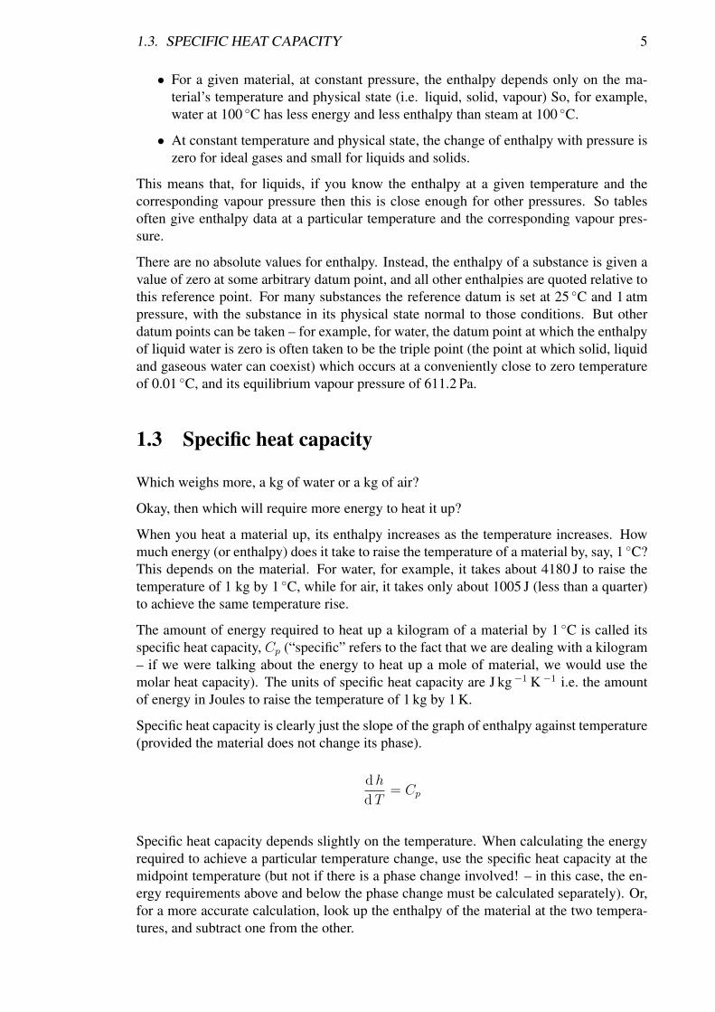
The amount of energy required to heat up a kilogram of a material by 1 ◦C is called itsspecific heat capacity, Cp (“specific” refers to the fact that we are dealing with a kilogram– if we were talking about the energy to heat up a mole of material, we would use themolar heat capacity). The units of specific heat capacity are J kg −1 K −1 i.e. the amountof energy in Joules to raise the temperature of 1 kg by 1 K.
Specific heat capacity is clearly just the slope of the graph of enthalpy against temperature(provided the material does not change its phase).
dh
dT= Cp
Specific heat capacity depends slightly on the temperature. When calculating the energyrequired to achieve a particular temperature change, use the specific heat capacity at themidpoint temperature (but not if there is a phase change involved! – in this case, the en-ergy requirements above and below the phase change must be calculated separately). Or,for a more accurate calculation, look up the enthalpy of the material at the two tempera-tures, and subtract one from the other.
6 CHAPTER 1. INTRODUCTION TO HEAT TRANSFER
T
hSlope = Cp
Figure 1.1: Specific heat capacity.
1.4 Rate of Energy Uptake
Specific heat capacity is the amount of energy required to raise the temperature of 1 kg ofmaterial by 1◦C; it has units of J kg−1 K−1. Looking at the units, if we multiply specificheat capacity by a temperature change and a mass flow rate, we will therefore get units ofJ s−1, i.e. Watts, or rate of heat transfer. The symbol for rate of heat transfer is Q (the dotindicates a flow rate):
Q = mCp (Tout − Tin)
W =Js
=kgs· J
kg K·K
So if we know the heat transfer rate, mass flow rate and specific heat capacity, we cancalculate the temperature change of a material from this equation.
The above equation is one of the most useful equations you’ll learn in this course. Thereis no need to memorise it, as you can work it out logically just by considering the unitsof specific heat capacity. But you do need to understand it – and by understanding it,naturally you’ll remember it.
For a batch operation the equation is much the same but without the dots, indicating thetotal quantity of energy required to change the temperature of a given mass:
Q = mCp (Tfinal − Tinitial)
J = kg · Jkg K
·K
Alternatively, the rate of change of temperature can be related to the heat transfer rate:
Q = mCpdT
d t
W = kg · Jkg K
· Ks
1.5 Latent heat of vaporisation/condensation (hfg) andlatent heat of fusion/melting (hsf )
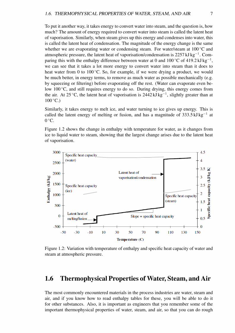
Water at atmospheric pressure boils when it reaches 100 ◦C, to form steam at 100 ◦C.Both are at the same temperature, but steam evidently contains more energy than water.
1.6. THERMOPHYSICAL PROPERTIES OF WATER, STEAM, AND AIR 7
To put it another way, it takes energy to convert water into steam, and the question is, howmuch? The amount of energy required to convert water into steam is called the latent heatof vaporisation. Similarly, when steam gives up this energy and condenses into water, thisis called the latent heat of condensation. The magnitude of the energy change is the samewhether we are evaporating water or condensing steam. For water/steam at 100 ◦C andatmospheric pressure, the latent heat of vaporisation/condensation is 2257 kJ kg−1. Com-paring this with the enthalpy difference between water at 0 and 100 ◦C of 419.2 kJ kg−1,we can see that it takes a lot more energy to convert water into steam than it does toheat water from 0 to 100 ◦C. So, for example, if we were drying a product, we wouldbe much better, in energy terms, to remove as much water as possible mechanically (e.g.by squeezing or filtering) before evaporating off the rest. (Water can evaporate even be-low 100 ◦C, and still requires energy to do so. During drying, this energy comes fromthe air. At 25 ◦C, the latent heat of vaporisation is 2442 kJ kg−1, slightly greater than at100 ◦C.)
Similarly, it takes energy to melt ice, and water turning to ice gives up energy. This iscalled the latent energy of melting or fusion, and has a magnitude of 333.5 kJ kg−1 at0 ◦C.
Figure 1.2 shows the change in enthalpy with temperature for water, as it changes fromice to liquid water to steam, showing that the largest change arises due to the latent heatof vaporisation.
Figure 1.2: Variation with temperature of enthalpy and specific heat capacity of water andsteam at atmospheric pressure.
1.6 Thermophysical Properties of Water, Steam, and Air
The most commonly encountered materials in the process industries are water, steam andair, and if you know how to read enthalpy tables for these, you will be able to do itfor other substances. Also, it is important as engineers that you remember some of theimportant thermophysical properties of water, steam, and air, so that you can do rough

8 CHAPTER 1. INTRODUCTION TO HEAT TRANSFER
calculations in your head or on an envelope. Table 1.1 shows typical values of importantthermophysical properties for water, steam and air. Note that values are given for differenttemperatures, either 0, 25, or 100 ◦C. The shaded values you ought to remember, at leastroughly – the others are there for reference. The density of air is not usually tabulated asit is easily calculated from the ideal gas law. Thermal conductivities and diffusivities aregiven for reference – we will introduce these later. Dynamic viscosities are also given,just for interest.
Table 1.1: Typical values of important thermophysical properties of water, ice, steam, and air.
Property Water Ice Steam AirSpecific heat capacity, Cp(kJ kg−1 K−1)
4.180a 2.101c 2.034b 1.005a
Latent heat of vaporisation/-condensation, hlg (kJ kg−1)
2257b 2257b
Latent heat of fusion/melting,hsl (kJ kg−1)
333.5c 333.5c
Density, ρ (kg m3) 997a– 958b 917c 0.6b 1.186a,*
Thermal conductivity, λ or k(W m−1 K−1)
0.611a 2.240c 0.0248b 0.025a
Viscosity, µ (Pa s) 891× 10−6a 12.06× 10⁻⁶b 18.3× 10⁻⁶a
Thermal diffusivity, α(m2 s−1)
0.147× 10⁻⁶a 1.17× 10⁻⁶c 20.3× 10⁻⁶b 21.0× 10⁻⁶a
Dynamic viscosity, v (m2 s−1)(= momentum diffusivity)
0.894× 10⁻⁶a 20.1× 10⁻⁶b 15.4× 10⁻⁶a
Ratiomomentum diffusivity
thermal diffusivity6.1a 0.99b 0.73a
a 25 ◦C, b 100 ◦C, c 0 ◦C, * From ideal gas law.Shaded values you ought to remember, at least approximately.
Figure 1.3 presents an abridged steam table, which list the important thermophysical prop-erties of liquid water and steam at selected temperatures and the corresponding saturatedvapour pressure.
Example: What is the energy requirement to raise the temperature of 60 kg of water from10 ◦C to 80 ◦C? Calculate the answer in two ways – by using the specific heat capacity atthe midpoint temperature (45 ◦C), and by subtracting the enthalpy of water at 10 ◦C fromthe enthalpy of water at 80 ◦C. Why are the two answers different? Which answer is moreaccurate?
Example: What is the energy requirement to convert 1 kg of water at 10 ◦C into steamat 150 ◦C? Calculate your answer by adding the energy required to raise the water from10 ◦C to 100 ◦C (using the specific heat capacity at the midpoint temperature of 55 ◦C),adding the latent heat of vaporisation, the adding the energy to raise the steam from 100 ◦Cto 150 ◦C (again using the appropriate mid-point temperature to look up the specific heatcapacity). Then calculate the energy requirement by subtracting the enthalpy of water at10 ◦C from the enthalpy of steam at 150 ◦C. How do the two answers compare?

1.7. CONSERVATION OF ENERGY AND ENERGY BALANCES 9
Figure 1.3: Abridged steam tables.
1.7 Conservation of energy and energy balances
Energy is expensive. An energy balance accounts for all the energy entering and leavinga system. If we overlook one of the forms of energy entering or leaving the system, wewill not calculate the energy balance correctly.
1.7.1 Energy balances
Conservation of energy is one of the fundamental laws of the universe, along with con-servation of mass, except where nuclear reactions are involved, in which case mass canbe converted to energy via the equation
E = mc2
Because c2 is such a large term, a very small amount of mass is converted into vastamounts of energy – this is why nuclear energy is such an attractive prospect.
10 CHAPTER 1. INTRODUCTION TO HEAT TRANSFER
1.7.2 Statement of the Law of Conservation
But in most process industries, except the nuclear industry, we don’t get nuclear reactionsoccurring, so we can take it as fundamentally true that energy, and mass, are conserved.This means that all the energy that enters a system must leave, one way or another, or elsemust accumulate in the system. We write this as follows:
IN− OUT + GENERATION− DISSIPATION = ACCUMULATION
This applies for heat transfer, mass transfer and momentum transfer. This is a fundamen-tal statement for chemical engineers, and it applies to all situations, from overall plantbalances to individual unit operations and to small elements within equipment. Applyingthis law to conservation of energy within process equipment results in sets of equations,either algebraic or differential, which describe the variation of temperature or heat flowwithin the equipment. If the process or operation involves no generation or dissipation ofheat (e.g. no reactions producing or removing energy), then the above equation simplifiesto
IN− OUT = ACCUMULATION
If the system is also operating at steady state i.e. nothing is changing, then there cannotbe any accumulation within the system, therefore
IN− OUT = 0
orTOTAL ENERGY IN = TOTAL ENERGY OUT
We must remember to include all forms of energy involved, and recognise that a particularform of energy is not necessarily conserved, as energy can be transformed, e.g. frommechanical work into heat.
It helps enormously when performing an energy balance (or a mass balance) to draw adashed line around the system of interest, whether the system is an entire process, somesection of it, a single unit operation, or a differential element within an item of processequipment. This helps to define clearly what energy flows are entering and leaving thesystem, and helps you to avoid overlooking any.
Mass and energy balance examples can be deceptively easy, but more difficult examplesrequire a systematic approach. Five helpful steps to performing mass and energy balancesare as follows:
1. Draw a picture, with all streams (mass and energy) entering and leaving the system.Draw a dashed line to indicate the boundaries of the system. Label the streams(with numbers if necessary).
2. Decide a basis on which to perform the calculations.
3. Draw up two balance tables, one for the mass balance, the other for the energybalance.
4. Perform preliminary calculations – fill in the balance tables.
5. Set x = the unknown quantity to be calculated. Solve for x.

1.7. CONSERVATION OF ENERGY AND ENERGY BALANCES 11
1.7.3 Temperature-Enthalpy Diagrams
You will remember the enthalpy-temperature diagram for water, where we showed howenthalpy changed with temperature. We showed it this way, because it makes intuitivesense to consider, when we change the temperature of water, how its enthalpy wouldchange. But it might actually be more sensible to look at it as, by adding energy to thewater, we are changing its enthalpy, and are seeing how the temperature changes. In otherwords, it might make more sense to make temperature the dependent axis, and enthalpythe independent axis. This would make our temperature-enthalpy diagram for a purecomponent look like Figure 1.4.
Figure 1.4: Temperature-enthalpy plot for a pure component at constant pressure.
TE is the temperature of evaporation, or the boiling point. For a multicomponent stream,this would vary over the evaporation region from the bubble point to the dew point.
TF is the temperature of fusion, or the freezing point. For a multicomponent stream, thiswould vary over the fusion region from the solidus point to the liquidus point.
hlg is the enthalpy (or latent heat) of evaporation = fn[T, P, composition] hsl is the en-thalpy (or latent heat) of fusion = fn[T, P, composition] hsg is the enthalpy (or latentheat) of sublimation = fn[T, P, composition]

12

Chapter 2General Heat Transfer Equation
Contents2.1 Introduction . . . . . . . . . . . . . . . . . . . . . . . . . . . . . . . 15
2.2 General Heat Transfer Equation . . . . . . . . . . . . . . . . . . . . 15
2.3 Mechanisms of Heat Transfer . . . . . . . . . . . . . . . . . . . . . . 16
2.3.1 Conduction . . . . . . . . . . . . . . . . . . . . . . . . . . . . 16
2.3.2 Convection . . . . . . . . . . . . . . . . . . . . . . . . . . . . 18
2.3.3 Radiation . . . . . . . . . . . . . . . . . . . . . . . . . . . . . 22
2.4 The Standard Engineering Equation, and Analogy with ElectricalCircuits . . . . . . . . . . . . . . . . . . . . . . . . . . . . . . . . . . 25
2.5 Problems . . . . . . . . . . . . . . . . . . . . . . . . . . . . . . . . . 29
13

14

2.1. INTRODUCTION 15
2.1 Introduction
We have talked a lot about energy balances, and that energy is conserved over a system,but may be transferred within the system. For example, in a heat exchanger the totalenergy entering and leaving the system is constant, but heat is transferred from the hot tothe cold stream. And we established that the rate of change of enthalpy of either stream,H & D , is equal in magnitude to the heat transfer rate, Q (in J s−1 or Watts, W), throughthe heat exchanger walls.
So energy balances tell us how much heat is transferred, but they do not tell us how (i.e.by what mechanisms) this heat is transferred, or how we can design our heat exchanger(or whatever) to achieve this rate of transfer. To decide these questions, we need to movefrom a study of energy balances to Heat Transfer.
2.2 General Heat Transfer Equation
Let us start by considering what factors we might expect to affect heat transfer. If I havean external wall in my office, with a window, and I lose heat through the wall and thewindow, what factors might affect the rate at which I lose heat and therefore the size ofthe heater I need in my office?
• size of the wall – Area, A
• temperature difference between my office and the outside – ∆T
• thickness of the wall – x
• what the wall is made of – its thermal conductivity – λ or k
• rate of transfer of heat from air inside to the wall, and from the wall to the outside
• Sunny, raining, windy
• Open or closed window
• etc.
In a general sense, the thing that is causing heat transfer to occur is the temperature dif-ference, ∆T
If ∆T is larger, the rate of heat transfer will be greater. The fact that there is a wall inthe way means that there is a resistance to heat transferring. If we have a thicker wall, forexample, the resistance to heat transfer will be greater, and heat will be transferred moreslowly. So the rate of heat transfer could be described by an equation:
Q =∆ t
R
where R incorporates all the factors that contribute to the resistance to heat transfer, suchas the area of the wall, its thickness, what it’s made of, etc. The units of R are clearlyK W−1, in other words, the amount of temperature driving force required to cause heat tobe transferred at a rate of 1 W. N.B. This is only true for steady state conditions.
Alternatively, the rate of heat transfer could be described by:
Q = UA∆T
16 CHAPTER 2. GENERAL HEAT TRANSFER EQUATION
where U represents some sort of overall heat transfer coefficient (units: W m−1 K−1),which would incorporate the thickness of the wall, what it’s made of, rate of heat transferto it from the air inside and from it to the air outside. Clearly, R = 1/UA.
This is the General Heat Transfer Equation, and ranks alongside Q = MCp (Tout − Tin) asone of the most important heat transfer equations you will learn – memorise it and digestit! The General Heat Transfer Equation can also be written as
q =Q
A= U∆T
where q is called the heat flux or heat transfer per unit area (units: W m−2). Often it is theheat flux that we are interested in.
2.3 Mechanisms of Heat Transfer
Let’s start by identifying the major energy transfer mechanisms.
Heat transfer Other energy transfer mechanismsConduction MechanicalConvection ElectricalRadiation Electromagnetic (e.g microwave)
(Phase change) Chemical reactionNuclear reaction
The difference between the heat transfer list and the other mechanisms identified abovefor energy transfer is that in the first list, the driving force for energy transfer is a tem-perature difference. For heat transfer, energy will only flow if there is a temperaturedifference. The other mechanisms can generate thermal energy within a material withoutthe requirement for a temperature gradient.
To quote from Ozisik, page 1, “Since heat flow takes places whenever there is a tem-perature gradient in a system, a knowledge of the temperature distribution in a system isessential in heat transfer studies.” We will therefore aim, as much as possible, to focus onwhat the temperature distribution is in the systems we are considering, i.e. the temperatureprofile.
2.3.1 Conduction
Conduction is the mechanism of heat transfer in which energy exchange takes place froma region of high temperature to one of lower temperature by the kinetic motion or directimpact of molecules and by the drift of electrons. The latter applies particularly to metals,which are both good electrical conductors and heat conductors. Essentially, conduction isheat transfer by molecular motion in solids or fluids at rest.
The empirical law of heat conduction, based on experimental observation, was proposedby Joseph Fourier, who stated that the rate of heat flow by conduction in a given directionis proportional to the area normal to the direction of heat flow and to the gradient of thetemperature in that direction:

2.3. MECHANISMS OF HEAT TRANSFER 17
Fourier’s law: Qx = −λAdT
dx
In terms of heat flux: qx = −λdT
dx
Qx is the rate of heat flow through area A in the positive x-direction. Heat will onlyflow in the positive x-direction if the temperature is decreasing in that direction – hencethe negative sign, as dT/dx must be negative for Qx to be positive – i.e. heat flows“downhill”. The proportionality constant, λ (or k as is often used) is called the thermalconductivity of the material. Good conductors have high values of λ, good insulatorslow values. λ has SI units W m−1 K−1, and varies from around 0.1 W m−1 K−1 for gasesand insulating materials to up to 1000 W m−1 K−1 for highly conducting metals such ascopper or silver. If the temperature gradient through the material is uniform (as it wouldbe in a slab of isotropic material) and at steady state, and the thermal conductivity doesnot change significantly with temperature, then Fourier’s equation can be written in itssteady state form:
Qx =λ
xA∆T
= UA∆T
=∆T
R
Therefore, U = λx
and R = xλA
for pure conduction.
Comparing with the General Heat Transfer Equation, we see that for pure conductionthrough a slab, U , the overall heat transfer coefficient, under steady state conditions isgiven by λ
x. If we think in terms of the resistance to heat transfer, then R = x
λA. This
makes sense: as the thickness of the wall increases, so must its resistance to heat transfer.But if the thermal conductivity is very large, then heat is transferred easily, and the resis-tance to heat transfer is small. Similarly, if the area is very large, then a lot of heat will belost through it.
Figure 2.1 overleaf shows typical ranges of thermal conductivities for various materials.Note that it is a logarithmic scale, and that metals have thermal conductivities typically1 000 − 10 000 times greater than insulators and gases. Figure 2.2 shows the effect oftemperature on thermal conductivities of some representative materials. Table 2.1 belowgives thermal conductivities of various materials at 0 ◦C.
18 CHAPTER 2. GENERAL HEAT TRANSFER EQUATION
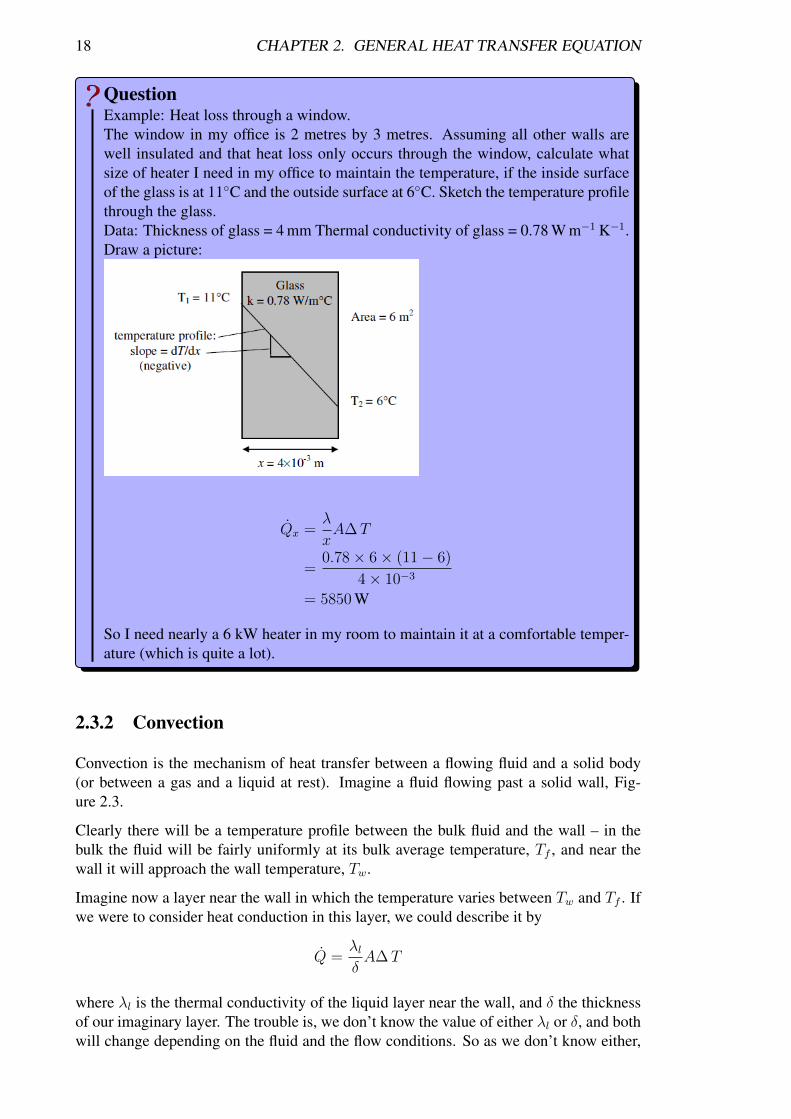
QuestionExample: Heat loss through a window.The window in my office is 2 metres by 3 metres. Assuming all other walls arewell insulated and that heat loss only occurs through the window, calculate whatsize of heater I need in my office to maintain the temperature, if the inside surfaceof the glass is at 11◦C and the outside surface at 6◦C. Sketch the temperature profilethrough the glass.Data: Thickness of glass = 4 mm Thermal conductivity of glass = 0.78 W m−1 K−1.Draw a picture:
Qx =λ
xA∆T
=0.78× 6× (11− 6)
4× 10−3
= 5850 W
So I need nearly a 6 kW heater in my room to maintain it at a comfortable temper-ature (which is quite a lot).
2.3.2 Convection
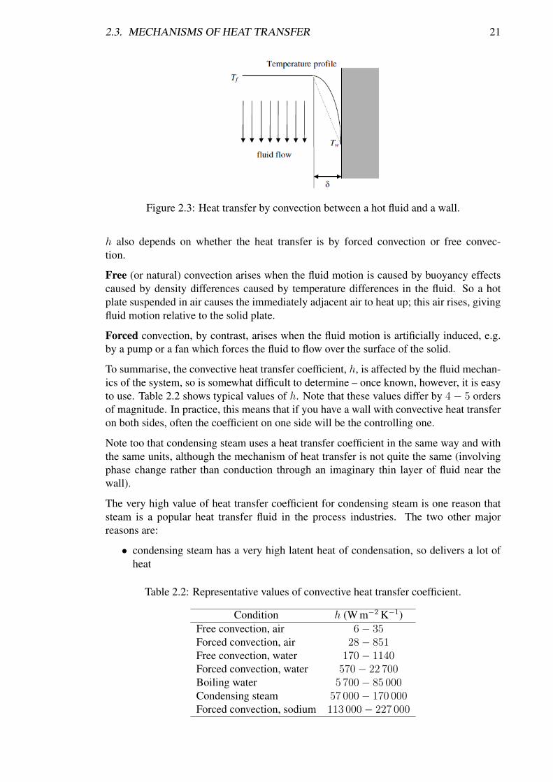
Convection is the mechanism of heat transfer between a flowing fluid and a solid body(or between a gas and a liquid at rest). Imagine a fluid flowing past a solid wall, Fig-ure 2.3.
Clearly there will be a temperature profile between the bulk fluid and the wall – in thebulk the fluid will be fairly uniformly at its bulk average temperature, Tf , and near thewall it will approach the wall temperature, Tw.
Imagine now a layer near the wall in which the temperature varies between Tw and Tf . Ifwe were to consider heat conduction in this layer, we could describe it by
Q =λlδA∆T
where λl is the thermal conductivity of the liquid layer near the wall, and δ the thicknessof our imaginary layer. The trouble is, we don’t know the value of either λl or δ, and bothwill change depending on the fluid and the flow conditions. So as we don’t know either,

2.3. MECHANISMS OF HEAT TRANSFER 19
Table 2.1: Thermal conductivities of various materials at 0 ◦C.
Material Thermal ConductivityW m−1 K−1 Btu −1hr −1ft ◦F−1
MetalsSilver (pure) 400 237Copper (pure) 385 223Aluminium (pure) 202 117Nickel (pure) 93 54Iron (pure) 73 42Carbon steel, 1% 43 25Lead (pure) 35 20.3Stainless steel (15% Cr, 10% Ni) 19 11.3Chrome-nickel steel (18% Cr, 8% Ni) 16.3 9.4Non-metallic solidsQuartz, parallel to axis 41.6 24Magnesite 4.15 2.4Marble 2.08− 2.94 1.2− 1.7Ice 2.0 1.19Sandstone 1.83 1.06Mortar 1.16 0.69Glass, window 0.78 0.45Maple or oak 0.17 0.096White pine 0.112 0.066Corrugated cardboard 0.064 0.038Sawdust 0.059 0.034Glass wool 0.038 0.022LiquidsMercury 8.21 4.74Water 0.556 0.327Ammonia 0.540 0.312Lubricating oil, SAE50 0.147 0.085Freon 12, CCl2F2 0.073 0.042GasesHydrogen 0.175 0.101Helium 0.141 0.081Air 0.024 0.0139Water vapour (saturated) 0.0206 0.0119Carbon dioxide 0.0146 0.00844
we may as well replace them both by a single term, which we will call the convective heattransfer coefficient, h:
Q = hA∆T
To be dimensionally correct, h must have SI units of W m−2 K−1. These are the sameunits as U ; clearly, for pure convection, U is equal to h. The resistance to heat transfer byconvection is given by R = 1/hA.
The convective heat transfer coefficient varies with the type of flow (turbulent or laminar),the geometry of the system, the physical properties of the fluid, the average temperature,the position along the surface of the body, and time. So calculating h is quite complicated.

20 CHAPTER 2. GENERAL HEAT TRANSFER EQUATION
Figure 2.1: Typical range of thermal conductivity of various materials.
Figure 2.2: Effect of temperature on thermal conductivity of materials.
We will consider ways to calculate it later in the course.
2.3. MECHANISMS OF HEAT TRANSFER 21
Figure 2.3: Heat transfer by convection between a hot fluid and a wall.
h also depends on whether the heat transfer is by forced convection or free convec-tion.
Free (or natural) convection arises when the fluid motion is caused by buoyancy effectscaused by density differences caused by temperature differences in the fluid. So a hotplate suspended in air causes the immediately adjacent air to heat up; this air rises, givingfluid motion relative to the solid plate.
Forced convection, by contrast, arises when the fluid motion is artificially induced, e.g.by a pump or a fan which forces the fluid to flow over the surface of the solid.
To summarise, the convective heat transfer coefficient, h, is affected by the fluid mechan-ics of the system, so is somewhat difficult to determine – once known, however, it is easyto use. Table 2.2 shows typical values of h. Note that these values differ by 4 − 5 ordersof magnitude. In practice, this means that if you have a wall with convective heat transferon both sides, often the coefficient on one side will be the controlling one.
Note too that condensing steam uses a heat transfer coefficient in the same way and withthe same units, although the mechanism of heat transfer is not quite the same (involvingphase change rather than conduction through an imaginary thin layer of fluid near thewall).
The very high value of heat transfer coefficient for condensing steam is one reason thatsteam is a popular heat transfer fluid in the process industries. The two other majorreasons are:
• condensing steam has a very high latent heat of condensation, so delivers a lot ofheat
Table 2.2: Representative values of convective heat transfer coefficient.
Condition h (W m−2 K−1)Free convection, air 6− 35Forced convection, air 28− 851Free convection, water 170− 1140Forced convection, water 570− 22 700Boiling water 5 700− 85 000Condensing steam 57 000− 170 000Forced convection, sodium 113 000− 227 000
22 CHAPTER 2. GENERAL HEAT TRANSFER EQUATION
• the temperature at which the steam condenses can be easily controlled by changingthe pressure
Additional, more minor, reasons include: steam is cheap, non-toxic, environmentallyfriendly
Example: Steam condenses on the inside of an insulated pipe 10 m in length and withouter diameter 5 cm. Heat is lost at a rate of 900 W to the external air at 15 ◦C with aconvective heat transfer coefficient of 20 W m−2 K−1. Calculate the temperature of theouter surface of the pipe.
Q = hAδ T
900 = 20× (π × 0.05× 10)× (Ts − 15)
Ts = 43.6 ◦C
Answer: 43.6 ◦C
2.3.3 Radiation
All bodies emit electromagnetic energy as a result of their temperature; this energy iscalled thermal radiation. The internal energy of the body is converted into electromag-netic waves which travel through space. The emitted radiation depends on the temper-ature of the body, the wave length (or range of wave lengths) and the condition of thesurface.
Similarly, radiation falling on a body may be absorbed, transmitted or reflected (or a com-bination of all three). Radiation incident on an absorbing body is attenuated as it passesthrough the body. If it is attenuated over a very short distance (a few angstroms), thenthe body is considered opaque to thermal radiation. Water and glass partially reflect, par-tially absorb and partially transmit, and are therefore considered semi-transparent. Onlyin a vacuum does thermal radiation propagate with no attenuation. However, air and mostgases are transparent to thermal radiation for most practical purposes, although somegases such as CO2, carbon monoxide, water vapour and ammonia can absorb significantthermal radiation over certain wavelength bands.
Bodies which absorb all radiation falling on them (without transmitting or reflecting any)are called black bodies. Black bodies are also perfect emitters or ideal radiators – theyemit the maximum possible amount of thermal radiation. Bodies which reflect or transmitsome of the radiation incident on them, and emit less than the maximum possible, arecalled grey bodies.
So, thermal radiation emitted from one body and absorbed by another represents a mech-anism of heat transfer. The difference between radiation and the other two forms of heattransfer discussed above, conduction and convection, is that radiation does not require amedium through which to travel. Radiation can transfer heat in a vacuum. This is howheat energy from the sun can travel to Earth, despite there being nothing (substantial) inbetween.
The maximum emitted radiation from a black body is given by the Stefan-Boltzmannlaw:
Eb = σT 4

2.3. MECHANISMS OF HEAT TRANSFER 23
where Eb is the emitted black body radiation (W m−2), T is the absolute temperature inKelvins (K), and σ is the Stefan-Boltzmann constant.
Clearly the amount of energy radiated by a body increases very rapidly with temperature,as this is raised to the fourth power.
Real (i.e. grey) bodies do not emit the maximum radiation given by the above equation,but some smaller amount given by
E = εEb = εσT 4
where ε is the emissivity of the surface.
The emissivity, ε, depends on the surface conditions. It is unity for a true black body, andbetween 0 and 1 for all real bodies.
When radiation falls onto a black body, it is completely absorbed. But for real (grey)bodies, the energy absorbed is less than all of the incident radiation, and is given by
qabs = αqinc
where qabs is the energy absorbed (W m−2), qinc is the energy incident on the surface(W m−2), and α is the absorptivity of the surface.
Like ε, α is between zero and unity, and is only unity for black bodies. The absorptivityof a body is generally different from its emissivity, but often, to simplify the analysis, αis assumed to equal ε.
The net heat transfer flux (heat transfer per unit area) for two very large black bodiesseparated by a vacuum is given by
q = Eb1 − Eb2= σ
(T 4
1 − T 42
)However, in real situations we are dealing with surfaces of finite areas which may beseparated such that not all of the radiation leaving one strikes the other. We are interestedin the net heat transfer in these situations, which we can describe by
Q = F1,2σA1
(T 4
1 − T 42
)where F1,2 is the view factor between the two surfaces which depends on the geometryof the system, and is defined as “the fraction of the radiation leaving surface 1 that isintercepted by surface 2”. This equation describes the heat transfer rate from a surface attemperature T1 of area A1 falling on a surface at temperature T2 and of area A2 (which isincluded in F1,2).
If one of the bodies is a black body or has a very large area (e.g. the sky), then (as we’llsee later) the equation simplifies to the following:
Q = σA1ε1
(T 4
1 − T 42
)This is the equation that we’ll use at this stage, as we’ll confine ourselves mostly togeometries where the area and emissivity of only one of the two bodies exchanging heatvia thermal radiation matters.
24 CHAPTER 2. GENERAL HEAT TRANSFER EQUATION
Heat transfer by thermal radiation is non-linear with respect to temperature. This can giverise to iterative calculations when combined with convection.
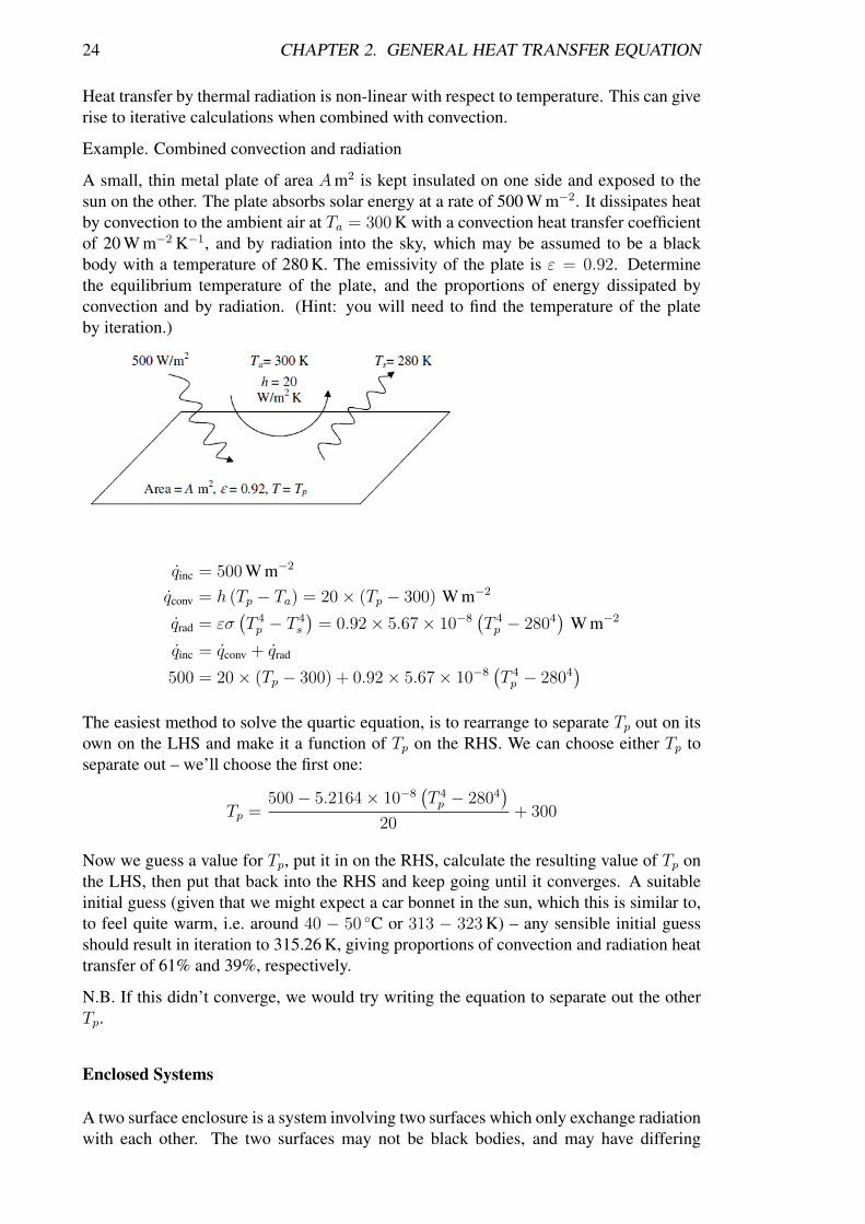
Example. Combined convection and radiation
A small, thin metal plate of area Am2 is kept insulated on one side and exposed to thesun on the other. The plate absorbs solar energy at a rate of 500 W m−2. It dissipates heatby convection to the ambient air at Ta = 300 K with a convection heat transfer coefficientof 20 W m−2 K−1, and by radiation into the sky, which may be assumed to be a blackbody with a temperature of 280 K. The emissivity of the plate is ε = 0.92. Determinethe equilibrium temperature of the plate, and the proportions of energy dissipated byconvection and by radiation. (Hint: you will need to find the temperature of the plateby iteration.)
qinc = 500 W m−2
qconv = h (Tp − Ta) = 20× (Tp − 300) W m−2
qrad = εσ(T 4p − T 4
s
)= 0.92× 5.67× 10−8
(T 4p − 2804
)W m−2
qinc = qconv + qrad
500 = 20× (Tp − 300) + 0.92× 5.67× 10−8(T 4p − 2804
)The easiest method to solve the quartic equation, is to rearrange to separate Tp out on itsown on the LHS and make it a function of Tp on the RHS. We can choose either Tp toseparate out – we’ll choose the first one:
Tp =500− 5.2164× 10⁻⁸
(T 4p − 2804
)20
+ 300
Now we guess a value for Tp, put it in on the RHS, calculate the resulting value of Tp onthe LHS, then put that back into the RHS and keep going until it converges. A suitableinitial guess (given that we might expect a car bonnet in the sun, which this is similar to,to feel quite warm, i.e. around 40 − 50 ◦C or 313 − 323 K) – any sensible initial guessshould result in iteration to 315.26 K, giving proportions of convection and radiation heattransfer of 61% and 39%, respectively.
N.B. If this didn’t converge, we would try writing the equation to separate out the otherTp.
Enclosed Systems
A two surface enclosure is a system involving two surfaces which only exchange radiationwith each other. The two surfaces may not be black bodies, and may have differing
2.4. THE STANDARD ENGINEERING EQUATION, AND ANALOGY WITH ELECTRICAL CIRCUITS25
emissivities. In this situation, the net heat transfer may be described by
Q =σ(T 4
1 − T 42
)1− ε1
ε1A1
+1
A1F1,2
+1− ε2
ε2A2
For large (infinite) parallel planes, where F1,2 = 1 and A1 = A2 = A, this simplifiesto
Q =σA(T 4
1 − T 42
)1
ε1
+1
ε2
− 1
while for long (infinite) concentric cylinders, where F1,2 = 1 and A1/A2 = r1/r2, thissimplifies to
Q =σA1
(T 4
1 − T 42
)1
ε1
+1− ε2
ε2
(r1
r2
)If one of the bodies is a black body or has a very large area (e.g. the sky), then the equationsimplifies to
Q = σA1ε1
(T 4
1 − T 42
)If a radiation shield of emissivities εs1 and εs2 on its two sides is inserted between twolarge parallel planes to reduce the heat transfer, it can be shown that the rate of heattransfer is then given by
Q =σA(T 4
1 − T 42
)(1
ε1
+1
ε2
− 1
)+
(1
εs1+
1
εs2− 1
)
If the emissivity of the shield is the same on both sides, this simplifies to
Q =σA(T 4
1 − T 42
)1
ε1
+2
εs+
1
ε2
− 2
and so on for additional shields.
2.4 The Standard Engineering Equation, and Analogywith Electrical Circuits
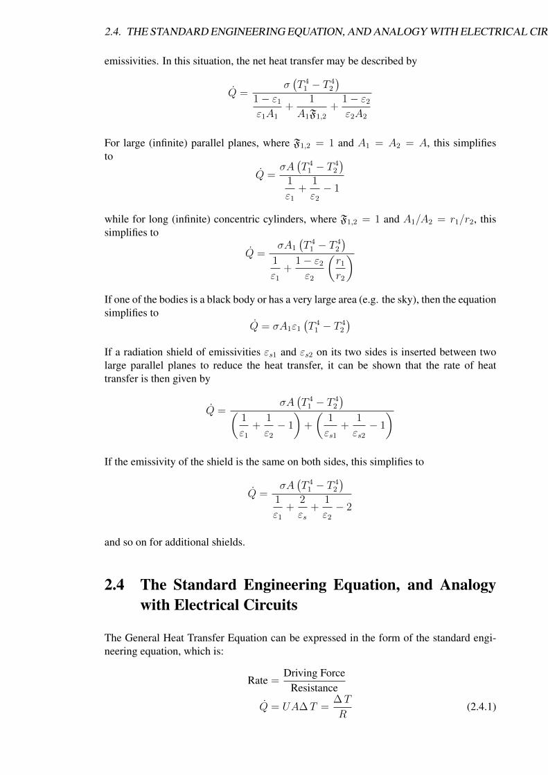
The General Heat Transfer Equation can be expressed in the form of the standard engi-neering equation, which is:
Rate =Driving Force
Resistance
Q = UA∆T =∆T
R(2.4.1)

26 CHAPTER 2. GENERAL HEAT TRANSFER EQUATION
where clearly, the resistance to heat transfer, R, is equal to 1/UA. Remember, this isonly true for steady state conditions; under unsteady state (i.e. changing) conditions, thedifferential form of the equation would need to be applied.
This form of equation is most familiar to us as
V = IR
or
I (rate of flow of electrons) =V (driving force)
R (resistance)
In fact, a circuit-type diagram can be drawn to represent heat transfer, as shown in Fig-ure 2.4.
Figure 2.4: Resistance diagram for heat transfer.
The concept of using circuit diagrams to represent heat transfer helps when we come toconsider several heat transfer operations in series, such as convection on one side of awall, conduction through the wall, and convection heat transfer from the other side. Itbecomes very clear that we determine the overall resistance by summing the individualresistances, as shown in Figure 2.5:
Figure 2.5: Summing heat transfer resistances in series, for convection and conductionthrough a wall.
From above
Q = UA∆T =(Ti − To)
R
2.4. THE STANDARD ENGINEERING EQUATION, AND ANALOGY WITH ELECTRICAL CIRCUITS27
where
R =1
UA
=1
A
(1
hi+x
λ+
1
ho
)As the areas for heat transfer are equal, we can simplify things by writing
Q = UA∆T
and calculating U directly from
1
U=
(1
hi+x
λ+
1
ho
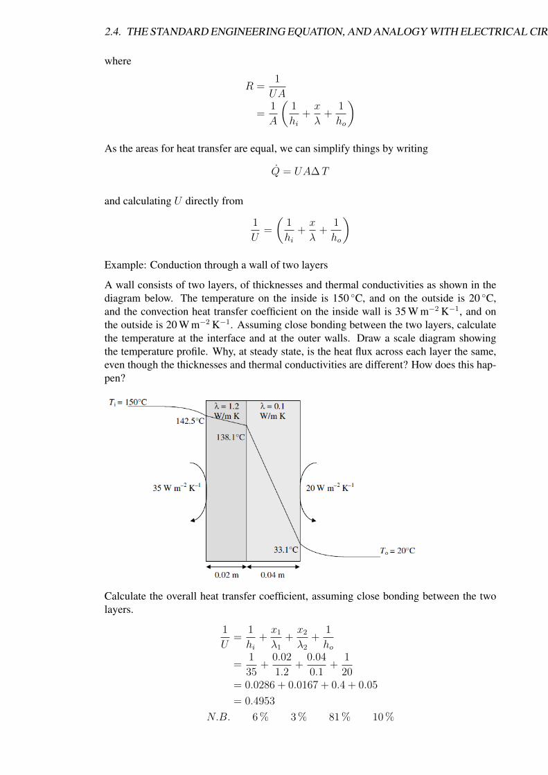
)Example: Conduction through a wall of two layers
A wall consists of two layers, of thicknesses and thermal conductivities as shown in thediagram below. The temperature on the inside is 150 ◦C, and on the outside is 20 ◦C,and the convection heat transfer coefficient on the inside wall is 35 W m−2 K−1, and onthe outside is 20 W m−2 K−1. Assuming close bonding between the two layers, calculatethe temperature at the interface and at the outer walls. Draw a scale diagram showingthe temperature profile. Why, at steady state, is the heat flux across each layer the same,even though the thicknesses and thermal conductivities are different? How does this hap-pen?
Calculate the overall heat transfer coefficient, assuming close bonding between the twolayers.
1
U=
1
hi+x1
λ1
+x2
λ2
+1
ho
=1
35+
0.02
1.2+
0.04
0.1+
1
20= 0.0286 + 0.0167 + 0.4 + 0.05
= 0.4953
N.B. 6 % 3 % 81 % 10 %
28 CHAPTER 2. GENERAL HEAT TRANSFER EQUATION
– most of the resistance is in the second layer.
U = 2.02 W m−2 K−1
Calculate the heat flux.
q = U∆T
= 2.02× (150− 20)
= 262.6 W m−2
Note – this same rate of heat transfer must pass from the inside to the wall, through eachlayer, and from the wall to the outside
Calculate the temperature at the left hand wall and at the interface between the two lay-ers.
q = hi∆T
262.6 = 35× (150− T1)
T1 = 142.5 ◦C
q =λ1
x1
∆T
262.6 =1.2
0.02× (142.5− T2)
T2 = 138.1 ◦C
Calculate the temperature at the right hand wall, and check that the final calculation yieldsa temperature of 20 ◦C.
q =λ2
x2
∆T
262.6 =0.1
0.04× (138.1− T3)
T2 = 33.1 ◦C
q = ho∆T
262.6 = 20× (33.1− T1)
T1 = 20 ◦C
Sketch the temperature profile on the above picture.
Why, at steady state, is the heat flux across each layer the same, even though the thick-nesses and thermal conductivities are different? How does this happen?
The heat flux must be the same across each layer, otherwise there would be accumulationof heat, the temperature would rise, and we would not be at steady state. How this isachieved is by matching the temperature driving force across each layer to the resistance– a layer with more resistance requires a larger temperature driving force to get the sameamount of heat through it. Remember the units of resistance, K W−1 i.e. the temperaturedriving force required to achieve 1 W of heat transfer. A larger resistance means a largertemperature driving force is required.
2.5. PROBLEMS 29
2.5 Problems
1. A tank of water is kept boiling with an internal 10 kW heater, and loses energythrough evaporation and through the walls of the tank. The surrounding environ-ment has a temperature of 20 ◦C.
(a) Calculate the heat loss through the walls, which are made of 5 mm thick stain-less steel with a total surface area of 2.8 m2. Calculate the percentage of re-sistance to heat transfer contributed by the boiling water, the walls and the air.Assume natural convection of the air. Which is the controlling resistance?
(b) Calculate the rate of evaporation of water.
Data:
Thermal conductivity of stainless steel = 19 W m−1 K−1
Latent heat of vaporisation of water = 2257 kJ kg−1
Take the convective heat transfer coefficient for boiling water to be about 45000W m−2 K−1, and for air under free convection to be 35 W m−2 K−1.
2. A thermocouple is located inside a ceramics oven for temperature control. Thewalls of the oven are at 600 ◦C, and the air temperature is 527 ◦C. The thermocouplecan be assumed to be spherical with a diameter of 2 mm, and to have a uniformtemperature throughout.
Assuming that both the oven walls and the thermocouple are black bodies withrespect to radiation, calculate the steady state temperature that would be recordedby the thermocouple for an air velocity of 4 m s−1 if the convection heat transfercoefficient can be found from the following correlation:
hD
l= 0.37Re0.6
Comment on the recorded measurements. Suggest how a more accurate air temper-ature reading could be obtained. [Hint: you will need to determine the steady statetemperature iteratively.]
Data: Physical properties of air at 527 ◦C
ρ = 0.435 kg m−3
µ = 0.370× 10⁻⁴ Pa s
λ = 0.0577 W m−1 K−1

30
Chapter 3Heat Transfer by Conduction
Contents3.1 Introduction . . . . . . . . . . . . . . . . . . . . . . . . . . . . . . . 33
3.2 Derivation of one-dimensional conduction heat transfer equation . . 33
3.2.1 Rectangular Coordinates . . . . . . . . . . . . . . . . . . . . . 36
3.2.2 Cylindrical Coordinates . . . . . . . . . . . . . . . . . . . . . 36
3.2.3 Spherical Coordinates . . . . . . . . . . . . . . . . . . . . . . 36
3.2.4 Special Cases . . . . . . . . . . . . . . . . . . . . . . . . . . . 36
3.2.5 Physical Meaning of the Laplace Equation . . . . . . . . . . . 38
3.3 Steady State Heat Conduction across a Slab . . . . . . . . . . . . . . 40
3.4 Steady State Heat Generation in a Slab Insulated on One Side . . . 42
3.5 Temperature Profiles across Cylindrical Walls . . . . . . . . . . . . 44
3.6 Temperature Profiles Across Spherical Walls . . . . . . . . . . . . . 47
3.7 Boundary Conditions . . . . . . . . . . . . . . . . . . . . . . . . . . 48
3.7.1 Prescribed Temperature Boundary Condition (First Kind) . . . . 48
3.7.2 Prescribed Heat Flux Boundary Condition (Second Kind) . . . . 48
3.7.3 Convection Boundary Condition (Third Kind) . . . . . . . . . . 49
3.8 Problems . . . . . . . . . . . . . . . . . . . . . . . . . . . . . . . . . 51
31

32

3.1. INTRODUCTION 33
3.1 Introduction
Conduction is the mechanism of heat transfer in solids. Solids tend to have temperaturedistributions or profiles across them, i.e. they are hotter on the outside or inside, or onone side etc. Fluids tend to be well-mixed, so that we are not really concerned abouttheir temperature distribution – it tends to even out to a uniform temperature just throughmixing. But solids don’t – heat is transferred by conduction, and the nature of the heattransfer depends on the temperature distribution. We noted earlier that “Since heat flowtakes places whenever there is a temperature gradient in a system, a knowledge of thetemperature distribution in a system is essential in heat transfer studies.” So we now wantto consider how to calculate firstly the temperature distribution in a system, and from itthe heat transfer rate.
3.2 Derivation of one-dimensional conduction heat trans-fer equation
To do this we will develop the basic mathematical equation which describes the temper-ature distribution through a system. We will do this based on the energy conservationequation, which we will apply to a very small element. As we noted earlier when wewere considering energy balances, conservation of energy applies whether we are con-sidering a whole plant, a single item of equipment, or a small differential element withinsome equipment. Here we are going to consider conservation of energy over a smalldifferential element.
To simplify the mathematical notation, and to illustrate the meaning of the terms in theequation, we will start by considering just one-dimensional conduction. This would applywhen considering, for example, conduction through a wall where the height and width ofthe wall are very large compared with its thickness, so that essentially there is no differ-ence in temperature along the height or width, and the only difference to be considered isthat across the thickness of the wall.
So, considering one-dimensional heat conduction in the x-dimension, consider a volumeelement of thickness ∆x and area normal to the x-direction, as shown in Figure 3.1 below.
Figure 3.1: Nomenclature for derivation of the one-dimensional heat conduction equation.

34 CHAPTER 3. HEAT TRANSFER BY CONDUCTION
An energy balance for this volume element is stated as(Net rate of heat gain
by conduction
)+
(Rate of
energy generation
)=
(Rate of increase
of internal energy
)I II = III
Note that this energy balance does not assume steady state, and it includes the possibilityof energy generation. This energy generation could arise from, for example, electricalresistance, nuclear reaction, or chemical reaction. Each of the terms I, II and III will beconsidered in turn.
I Net rate of heat gain by conduction
Heat enters the volume element by conduction through the area A normal to the x-coordinate at the point x, and leaves by conduction through the area A at the pointx+ ∆x. Let q be the conduction heat flux (heat flow per unit area, W m2) at point xin the positive x-direction at the surface A of the element. Then the rate of heat flowinto the volume element through the surface A at location x is written as
[Aq]x
Similarly, the rate of heat flow out of the element by conduction at the location x +∆x is given by
[Aq]x+∆x
Then the net rate of heat flow by conduction into the element is the difference be-tween the flow in and flow out:
I ≡ [Aq]x − [Aq]x+∆x
II Rate of energy generation
The rate of energy generation in an element of volume ADx is given by
II ≡ A∆xg
where g = g(x, t) is the energy generation per unit volume (W m3) at the point x andat time t.
III Rate of increase of internal energy
The relationship between the rate of energy input into a mass of material and the rateof energy change is given by
Q = mCpdT
d tkg× J
kg K× K
s= W
Mass is given by density × volume, therefore
III ≡ A∆xρCp∂ T (x, t)
∂ t
Note that we use the partial derivative, ∂, as we are considering in the term the changein temperature with respect to time, but not distance.
3.2. DERIVATION OF ONE-DIMENSIONAL CONDUCTION HEAT TRANSFER EQUATION35
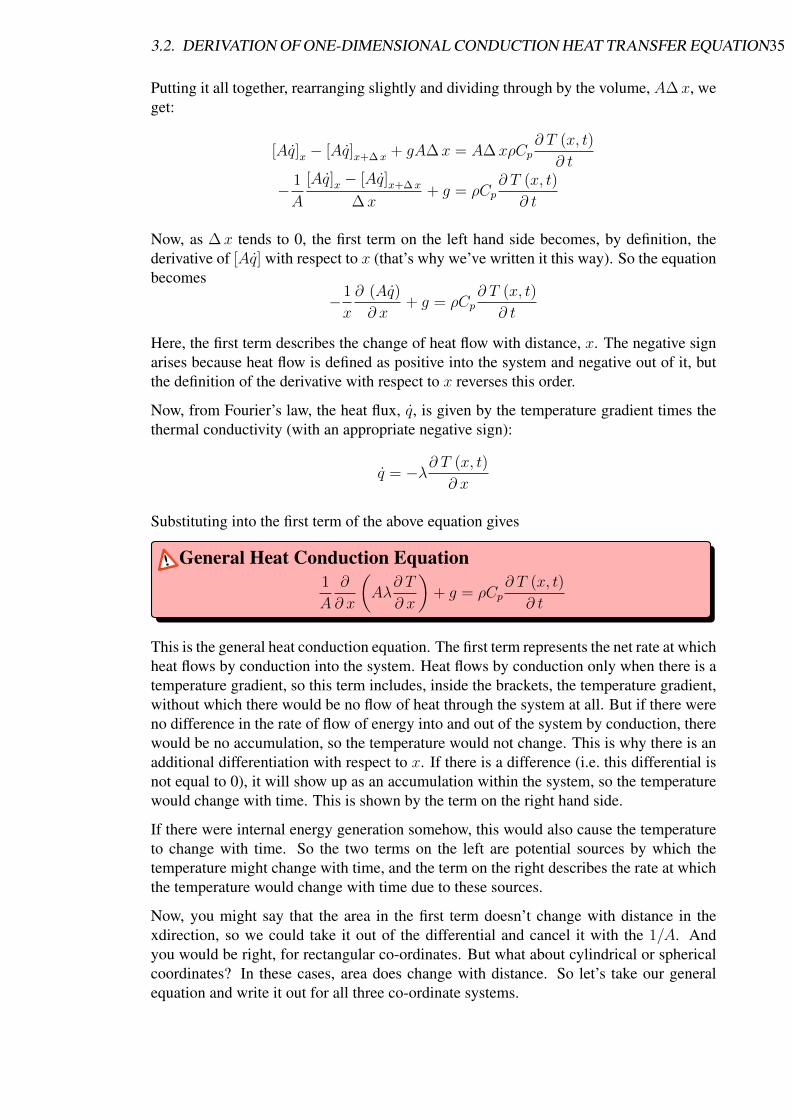
Putting it all together, rearranging slightly and dividing through by the volume, A∆x, weget:
[Aq]x − [Aq]x+∆x + gA∆x = A∆xρCp∂ T (x, t)
∂ t
− 1
A
[Aq]x − [Aq]x+∆x
∆x+ g = ρCp
∂ T (x, t)
∂ t
Now, as ∆x tends to 0, the first term on the left hand side becomes, by definition, thederivative of [Aq] with respect to x (that’s why we’ve written it this way). So the equationbecomes
−1
x
∂ (Aq)
∂ x+ g = ρCp
∂ T (x, t)
∂ t
Here, the first term describes the change of heat flow with distance, x. The negative signarises because heat flow is defined as positive into the system and negative out of it, butthe definition of the derivative with respect to x reverses this order.
Now, from Fourier’s law, the heat flux, q, is given by the temperature gradient times thethermal conductivity (with an appropriate negative sign):
q = −λ∂ T (x, t)
∂ x
Substituting into the first term of the above equation gives
General Heat Conduction Equation1
A
∂
∂ x
(Aλ
∂ T
∂ x
)+ g = ρCp
∂ T (x, t)
∂ t
This is the general heat conduction equation. The first term represents the net rate at whichheat flows by conduction into the system. Heat flows by conduction only when there is atemperature gradient, so this term includes, inside the brackets, the temperature gradient,without which there would be no flow of heat through the system at all. But if there wereno difference in the rate of flow of energy into and out of the system by conduction, therewould be no accumulation, so the temperature would not change. This is why there is anadditional differentiation with respect to x. If there is a difference (i.e. this differential isnot equal to 0), it will show up as an accumulation within the system, so the temperaturewould change with time. This is shown by the term on the right hand side.
If there were internal energy generation somehow, this would also cause the temperatureto change with time. So the two terms on the left are potential sources by which thetemperature might change with time, and the term on the right describes the rate at whichthe temperature would change with time due to these sources.
Now, you might say that the area in the first term doesn’t change with distance in thexdirection, so we could take it out of the differential and cancel it with the 1/A. Andyou would be right, for rectangular co-ordinates. But what about cylindrical or sphericalcoordinates? In these cases, area does change with distance. So let’s take our generalequation and write it out for all three co-ordinate systems.
36 CHAPTER 3. HEAT TRANSFER BY CONDUCTION
3.2.1 Rectangular Coordinates
These are our familiar, Cartesian, x, y, z coordinates, and in this system of coordinates,area normal to the x-direction does not change as x increases. SoA in the general equationis constant, and the equation simplifies to
∂
∂ x
(λ∂ T
∂ x
)+ g = ρCp
∂ T (x, t)
∂ t
This is the one-dimensional, time-dependent heat conduction equation in the rectangularcoordinate system.
3.2.2 Cylindrical Coordinates
In cylindrical co-ordinates our three axes are given by r, φ, and z, and for one-dimensionalheat conduction we are concerned with conduction in the radial direction, r. Area in-creases proportionally with r, so the general equation becomes
1
r
∂
∂ r
(rλ∂ T
∂ r
)+ g = ρCp
∂ T (r, t)
∂ t
This is the one-dimensional, time-dependent heat conduction equation in the cylindricalcoordinate system.
3.2.3 Spherical Coordinates
In spherical co-ordinates, once again we denote the radial coordinate by r instead of x. Inthis case, area A is proportional to r2, so the general equation becomes
1
r2
∂
∂ r
(r2λ
∂ T
∂ r
)+ g = ρCp
∂ T (r, t)
∂ t
This is the one-dimensional, time-dependent heat conduction equation in spherical coor-dinates.
3.2.4 Special Cases
Let’s consider some special cases, which will help us understand what each of the termsmeans in a physical sense. And, to avoid excessive brain strain, let’s look just at thefamiliar rectangular co-ordinate system, for which the equation is
∂
∂ x
(λ∂ T
∂ x
)+ g = ρCp
∂ T (x, t)
∂ t

3.2. DERIVATION OF ONE-DIMENSIONAL CONDUCTION HEAT TRANSFER EQUATION37
Constant Thermal Conductivity
If the thermal conductivity, λ, were constant, then we could take it out of the first term.We could also divide through by λ, to give
∂
∂ x
(∂ T
∂ x
)+g
λ=ρCpλ
∂ T (x, t)
∂ t
∂2 T
∂ x2 +g
λ=
1
α
∂ T
∂ t
where α is the thermal diffusivity (λ/ρCp). The thermal diffusivity is a measure of therate at which heat is propagated through a medium; the larger the thermal diffusivity, thefaster heat is propagated.
No Internal Energy Generation
If, in addition, there were no internal energy generation, and we were just consideringpure conduction heat transfer, then we get
∂2 T
∂ x2 =1
α
∂ T
∂ tFourier Equation
This means quite simply that the rate of change of temperature, which indicates a rate ofchange of internal energy, must be balanced by the net rate at which energy is flowing byconduction into the system.
No Heat Conduction
If both surfaces of the system were well insulated so that there was no conduction into orout of the element, then the equation becomes
g
λ=
1
α
∂ T
∂ t
which is equivalent to
g = ρCp∂ T
∂ t
then multiply both sides by m3 to get
Power (W) = mCp∂ T
∂ t
This quite clearly means that the rate of energy generation is balanced by the rate ofchange of temperature of the material.

38 CHAPTER 3. HEAT TRANSFER BY CONDUCTION
Steady State Heat Conduction
Under steady state conditions, there is no change with respect to time. Therefore the righthand side of the above equation must be zero:
d2 T
dx2 +g
λ= 0 Poisson Equation
Note that for steady state conditions the derivatives are no longer partial, so d is usedinstead of ∂.
If there is also no internal energy generation, then
d2 T
dx2 = 0 Laplace Equation
This is the Laplace equation, and it simply means that, while there is a temperature gradi-ent causing conduction heat flow (i.e. the first derivative is not zero), there is no differencein the heat flow that would cause accumulation (i.e. the second differential does equalzero), so there is no accumulation and therefore no temperature change.
If there is internal energy generation, then the Poisson equation simply means that the rateof internal energy generation is balanced by the rate of conduction out of the system, andthere is no accumulation and no temperature change.
Equivalent equations exist for cylindrical and spherical co-ordinates (see below), and forthree-dimensional heat conduction. For three dimensional steady state heat conductionwith no internal energy generation, Laplace’s equation becomes
∂2 T
∂ x2 +∂2 T
∂ y2 +∂2 T
∂ z2 = ∇2T = 0
which is the three-dimensional form of Laplace’s equation.
Table 3.1: Summary of the Poisson and Laplace equations in different coordinate systems.
Coordinate System Poisson equation Laplace equation
Rectangulard2 T
dx2 +g
λ= 0
d2 T
dx2 = 0
Cylindrical1
r
d
d r
(r
dT
d r
)+g0
λ= 0
d
d r
(r
dT
d r
)= 0
Spherical1
r2
d
d r
(r2 dT
d r
)+g0
λ= 0
d
d r
(r2 dT
d r
)= 0
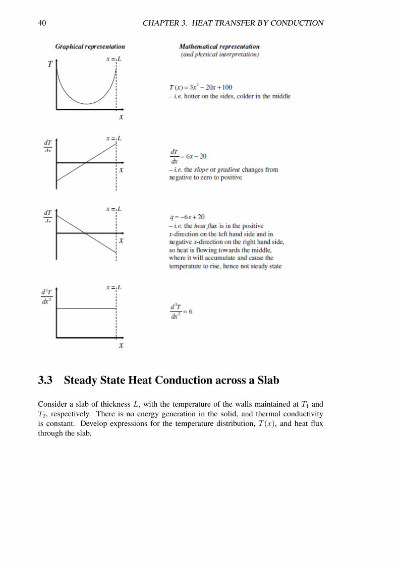
3.2.5 Physical Meaning of the Laplace Equation
Heat flow by conduction is proportional to the temperature gradient...

3.2. DERIVATION OF ONE-DIMENSIONAL CONDUCTION HEAT TRANSFER EQUATION39
There will only be accumulation of heat if the temperature gradient changes...
Let’s think about the relationship between the physical situation and the mathematicsdescribing that physical situation a bit further. The figure below shows an instantaneoustemperature profile in a solid slab of thickness L. The temperature profile might arise, forexample, because the slab has been plunged into hot water such that the sides have begunto heat, while the centre is still cool. Eventually the whole slab will heat to the sameuniform temperature throughout, but at a given moment in time, the temperature profileis as shown in the figure. For the sake of illustration, it can be described by a quadraticfunction, as shown to the right of the figure.
Sketch the profiles of dT/dx, q and d2T/dx2 across the slab, based on thinking aboutwhat is going on physically as indicated by the figure, and based on differentiating themathematical expression describing the physical situation. To simplify the maths, assumeλ = 1 W m−1 K−1.
40 CHAPTER 3. HEAT TRANSFER BY CONDUCTION
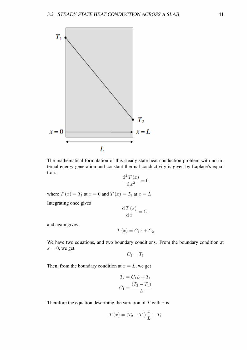
3.3 Steady State Heat Conduction across a Slab
Consider a slab of thickness L, with the temperature of the walls maintained at T1 andT2, respectively. There is no energy generation in the solid, and thermal conductivityis constant. Develop expressions for the temperature distribution, T (x), and heat fluxthrough the slab.
3.3. STEADY STATE HEAT CONDUCTION ACROSS A SLAB 41
The mathematical formulation of this steady state heat conduction problem with no in-ternal energy generation and constant thermal conductivity is given by Laplace’s equa-tion:
d2 T (x)
dx2 = 0
where T (x) = T1 at x = 0 and T (x) = T2 at x = L
Integrating once givesdT (x)
dx= C1
and again givesT (x) = C1x+ C2
We have two equations, and two boundary conditions. From the boundary condition atx = 0, we get
C2 = T1
Then, from the boundary condition at x = L, we get
T2 = C1L+ T1
C1 =(T2 − T1)
L
Therefore the equation describing the variation of T with x is
T (x) = (T2 − T1)x
L+ T1

42 CHAPTER 3. HEAT TRANSFER BY CONDUCTION
which is a straight line starting at T1, with slope (T2 − T1)/L. If T2 < T1, then this slopeis negative, and heat flows from T1 to T2.
So we know the temperature distribution. But we want to know the heat flowrate or flux.This we get from Fourier’s law:
q = −λdT
dx
Differentiating our temperature distribution with respect to x gives
dT
dx=
(T2 − T1)
L
Thereforeq (x) = −λ
L(T2 − T1)
orQ =
λ
LA∆T
which is the same (essentially) as the conduction heat transfer equation which we devel-oped earlier. Note that q(x) is independent of x, i.e. is the same throughout the slab.
So we have learned from this exercise that we solve the general heat conduction equationby integrating, and we find the constants of integration from the boundary conditions.We therefore need as many boundary conditions as constants of integration (two in thiscase). We have also learned that, having found the temperature distribution in this way, wedifferentiate it to find the heat flux, and that the equation obtained in this way is the sameas that which we encountered earlier for describing heat conduction through a slab – inother words, what we are learning now is no different to what we learned about conductionearlier, it’s just that we’ve made the fundamental basis for it more explicit.
3.4 Steady State Heat Generation in a Slab Insulated onOne Side
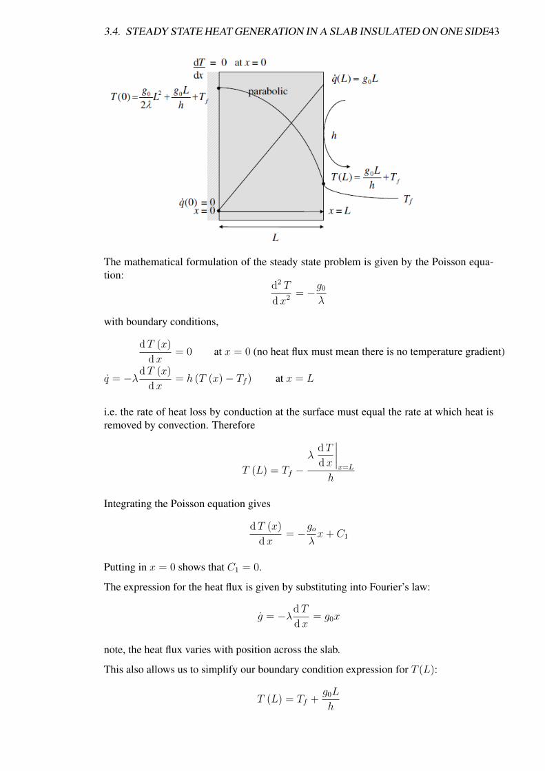
Consider a slab of thickness L and constant thermal conductivity λ in which energy isgenerated at a constant rate of g0 W m3. The boundary surface at x = 0 is insulatedso that there is no heat flow across this boundary, and that at x = L dissipates heat byconvection into a fluid at temperature Tf with a heat transfer coefficient h.
In this example, there is energy generation in the medium. This could apply to an electri-cal heating element or a nuclear fuel rod, for example. This means that we are unable tocalculate the heat flow by considering the driving force and resistance to flow – we cannotuse the resistance approach when there is energy generation. To solve this one, we needto solve the heat conduction equation.
3.4. STEADY STATE HEAT GENERATION IN A SLAB INSULATED ON ONE SIDE43
The mathematical formulation of the steady state problem is given by the Poisson equa-tion:
d2 T
dx2 = −g0
λ
with boundary conditions,
dT (x)
dx= 0 at x = 0 (no heat flux must mean there is no temperature gradient)
q = −λdT (x)
dx= h (T (x)− Tf ) at x = L
i.e. the rate of heat loss by conduction at the surface must equal the rate at which heat isremoved by convection. Therefore
T (L) = Tf −λ
dT
dx
∣∣∣∣x=L
h
Integrating the Poisson equation gives
dT (x)
dx= −go
λx+ C1
Putting in x = 0 shows that C1 = 0.
The expression for the heat flux is given by substituting into Fourier’s law:
g = −λdT
dx= g0x
note, the heat flux varies with position across the slab.
This also allows us to simplify our boundary condition expression for T (L):
T (L) = Tf +g0L
h
44 CHAPTER 3. HEAT TRANSFER BY CONDUCTION
Integrating again givesT (x) = − go
2λx2 + C2
Applying the boundary condition at x = L gives
T (L) = − go2λL2 + C2 = Tf +
g0L
h
ThereforeC2 =
go2λL2 +
g0L
h+ Tf
Therefore the temperature distribution becomes
T (x) = − go2λx2 +
go2λL2 +
g0L
h+ Tf
=go2λL2
(1−
(xL
)2)
+g0L
h+ Tf
The physical significance of these terms is that the first is due to the energy generation,and the second to the presence of the finite convection heat transfer coefficient at thesurface. If this were infinite, this term would vanish.
Note that the temperature distribution is not uniform across the slab (it is parabolic), andneither is the heat flux (which is linear with respect to x, starting at 0).
3.5 Temperature Profiles across Cylindrical Walls
Cylindrical systems are very frequently encountered in the process industries, in partic-ular in pipework. Often we have pipes conveying hot fluids, and it is important that weknow the temperature distribution and therefore heat losses across the pipe walls. Otherexamples include heat generation in cylindrical fuel elements in nuclear reactors or inelectrical wires carrying currents.
The steady state heat conduction equation with constant, uniform energy generation forthe cylindrical co-ordinate system is given by
1
r
d
d r
(r
dT
d r
)+g0
λ= 0
or,d
d r
(r
dT
d r
)= −g0
λr
Integrating twice gives
dT (r)
d r= − g0
2λr +
C1
r
T (r) = − g0
4λr2 + C1 ln r + C2
Clearly, we need two boundary conditions to determine the two integration constants.

3.5. TEMPERATURE PROFILES ACROSS CYLINDRICAL WALLS 45
To solve this for a solid cylinder with energy generation (e.g. a wire carrying current), wewould specify the surface temperature and that the heat flux at the centre of the wire = 0,due to the temperature gradient at the centre being 0 (as the cylinder is symmetric).
Let us consider the more common (for process engineers) situation of a hollow pipewith no internal energy generation containing flowing fluid, where the inner surface atr = ri and the outer surface at r = ro are maintained at temperatures Ti and To, respec-tively.
Therefore the above equations become
dT (r)
d r=C1
rT (r) = C1 ln r + C2
The boundary conditions give us
Ti = C1 ln ri + C2
To = C1 ln ro + C2
Simultaneous solution of these equations gives
C1 =To − Ti
ln
(rori
)C2 = Ti − (To − Ti)
ln ri
ln
(rori
)Introducing these into the above equation for T (r) gives
T (r) =To − Ti
ln
(rori
) ln r + Ti − (To − Ti)ln ri
ln
(rori
)= Ti + (To − Ti)
ln r − ln ri
ln
(rori
)from which
T (r)− TiTo − Ti
=
ln
(r
ri
)ln
(rori
)
46 CHAPTER 3. HEAT TRANSFER BY CONDUCTION
The heat flux is given, as usual, by Fourier’s law:
q = −λdT (r)
d r
From earlier,dT (r)
d r=C1
r=
1
r
To − Ti
ln
(rori
)Hence
q =λ
r
Ti − To
ln
(rori
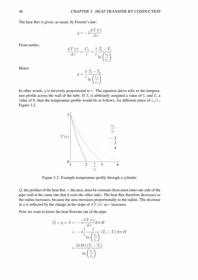
)In other words, q is inversely proportional to r. The equation above tells us the tempera-ture profile across the wall of the tube. If Ti is arbitrarily assigned a value of 1, and To avalue of 0, then the temperature profile would be as follows, for different ratios of ro/ri,Figure 3.2.
T (r)
r
ri
rori
234
1
01 2 3 4
Figure 3.2: Example temperature profile through a cylinder.
Q, the product of the heat flux× the area, must be constant (heat must enter one side of thepipe wall at the same rate that it exits the other side). The heat flux therefore decreases asthe radius increases, because the area increases proportionally to the radius. The decreasein q is reflected by the change in the slope of dT/d r as r increases.
Now we want to know the heat flowrate out of the pipe:
Q = q × A = − λdT (r)
d r2πrH
= − λ1
r
1
ln
(rori
) (To − Ti) 2πrH
=2πHλ (Ti − To)
ln
(rori
)

3.6. TEMPERATURE PROFILES ACROSS SPHERICAL WALLS 47
Comparing with
Q =(Ti − To)
R
clearly, the resistance to heat transfer is given by
R =1
UA=
ln
(rori
)2πHλ
This analysis is appropriate when the thickness of the pipe walls is large compared withthe pipe radius. For thin-walled pipes (where the pipe thickness is small compared withthe radius), a rectangular approximation can be used.
Alternatively, the log-mean area, Am, can be used, defined by
R =x
λAm=
(ro − ri)λAm
=
ln
(rori
)2πHλ
Am =(ro − ri) 2πH
ln
(rori
) =(Ao − Ai)
ln
(AoAi
)
The log-mean area will be useful for heat exchanger calculations.
3.6 Temperature Profiles Across Spherical Walls
Spherical or hemi-spherical shaped containers are often used in the process industries,because the have the minimum surface area per unit volume (so minimise heat losses)and have uniform distribution of stresses within the container walls. It is left as a tutorialexercise for students to show that the temperature distribution across the wall of a hollowspherical container of constant thermal conductivity, with inner and outer surfaces main-tained at temperatures Ti and To respectively, for steady state heat conduction with nointernal energy generation, is given by
T (r) =rir
ro − rro − ri
Ti +ror
r − riro − ri
To
and the heat flow byQ = 4πλ
riroro − ri
(Ti − To)
The resistance can then given by
R =1
4πλ
ro − ririro
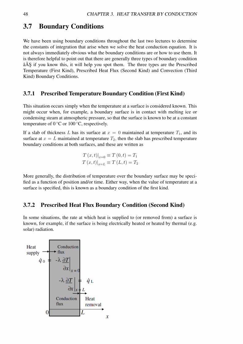
48 CHAPTER 3. HEAT TRANSFER BY CONDUCTION
3.7 Boundary Conditions
We have been using boundary conditions throughout the last two lectures to determinethe constants of integration that arise when we solve the heat conduction equation. It isnot always immediately obvious what the boundary conditions are or how to use them. Itis therefore helpful to point out that there are generally three types of boundary conditionâAS if you know this, it will help you spot them. The three types are the PrescribedTemperature (First Kind), Prescribed Heat Flux (Second Kind) and Convection (ThirdKind) Boundary Conditions.
3.7.1 Prescribed Temperature Boundary Condition (First Kind)
This situation occurs simply when the temperature at a surface is considered known. Thismight occur when, for example, a boundary surface is in contact with melting ice orcondensing steam at atmospheric pressure, so that the surface is known to be at a constanttemperature of 0 ◦C or 100 ◦C, respectively.
If a slab of thickness L has its surface at x = 0 maintained at temperature T1, and itssurface at x = L maintained at temperature T2, then the slab has prescribed temperatureboundary conditions at both surfaces, and these are written as
T (x, t)|x=0 ≡ T (0, t) = T1
T (x, t)|x=L ≡ T (L, t) = T2
More generally, the distribution of temperature over the boundary surface may be speci-fied as a function of position and/or time. Either way, when the value of temperature at asurface is specified, this is known as a boundary condition of the first kind.
3.7.2 Prescribed Heat Flux Boundary Condition (Second Kind)
In some situations, the rate at which heat is supplied to (or removed from) a surface isknown, for example, if the surface is being electrically heated or heated by thermal (e.g.solar) radiation.
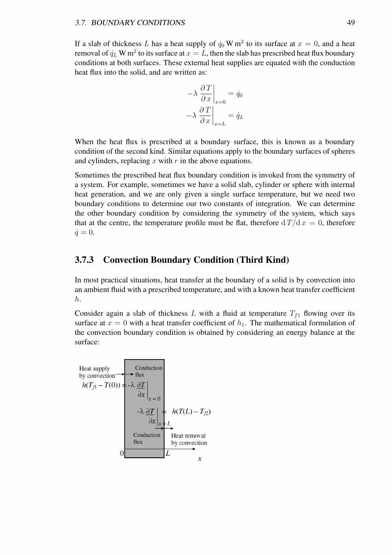
3.7. BOUNDARY CONDITIONS 49
If a slab of thickness L has a heat supply of q0 W m2 to its surface at x = 0, and a heatremoval of qL W m2 to its surface at x = L, then the slab has prescribed heat flux boundaryconditions at both surfaces. These external heat supplies are equated with the conductionheat flux into the solid, and are written as:
−λ ∂ T∂ x
∣∣∣∣x=0
= q0
−λ ∂ T∂ x
∣∣∣∣x=L
= qL
When the heat flux is prescribed at a boundary surface, this is known as a boundarycondition of the second kind. Similar equations apply to the boundary surfaces of spheresand cylinders, replacing x with r in the above equations.
Sometimes the prescribed heat flux boundary condition is invoked from the symmetry ofa system. For example, sometimes we have a solid slab, cylinder or sphere with internalheat generation, and we are only given a single surface temperature, but we need twoboundary conditions to determine our two constants of integration. We can determinethe other boundary condition by considering the symmetry of the system, which saysthat at the centre, the temperature profile must be flat, therefore dT/dx = 0, thereforeq = 0.
3.7.3 Convection Boundary Condition (Third Kind)
In most practical situations, heat transfer at the boundary of a solid is by convection intoan ambient fluid with a prescribed temperature, and with a known heat transfer coefficienth.
Consider again a slab of thickness L with a fluid at temperature Tf1 flowing over itssurface at x = 0 with a heat transfer coefficient of h1. The mathematical formulation ofthe convection boundary condition is obtained by considering an energy balance at thesurface:
50 CHAPTER 3. HEAT TRANSFER BY CONDUCTION
Convection heat fluxfrom the fluid at Tf1 to
the surface at x = 0
=
Conduction heat fluxfrom the surface atx = 0 into the plate
h1 [Tf1 − T (x, t)|x=0] = − λ ∂ T
∂ x
∣∣∣∣x=0
If a fluid at temperature Tf2 with heat transfer coefficient h2 flows over the surface atx = L, the energy balance is staged as
h2 [T (x, t)|x=L − Tf2] = −λ ∂ T∂ x
∣∣∣∣x=L
A convection boundary condition is known as a boundary condition of the third kind. Theconvection boundary condition is the most general of the three – in fact, the other twoare just special cases (see Ozisik for the reasoning why). The solution of conduction heattransfer problems hinges on the boundary conditions, and these are usually convectionboundary conditions. This means that the next key to solving heat transfer problems isknowing how to calculate the convection heat transfer coefficient.

3.8. PROBLEMS 51
3.8 Problems
1. A commercial freezer is to be maintained at −18 ◦C. The freezer is insulated withglass wool insulation sandwiched between two sheets of aluminum. Calculate thethickness of glass wool insulation required (λ = 0.04 W m−1 K−1) if the externalwall temperature is 25 ◦C, and the heat flux into the freezer is 170 W m−2. Ignorethe thermal resistance of the aluminum sheets. How will a variation of 1 ◦C in theexternal wall temperature impact on the thickness of insulation required?
[1 cm]
2. A furnace wall is made up of three layers, the inner one of firebrick, the middleone of insulating brick and the outer one of red brick, of thermal conductivities1.21, 0.13, and 0.85 W m−1 K−1, respectively, and thicknesses 200 mm, 70 mm, and95 mm, respectively. The inner wall is at 900 ◦C, and the heat flux is 1000 W m−2.Assuming close bonding between each layer at their interfaces, calculate the tem-perature at each interface and at the outer wall. Is the outer wall at a safe tem-perature for nearby personnel? Which is the controlling resistance? Draw a scalediagram showing the temperature profile.
[900 ◦C, 735 ◦C, 196 ◦C, 84 ◦C]
3. A stainless steel fermentation vessel is to be maintained at 37 ◦C. The vessel hasa cylindrical central section 2 m in diameter and 3 m in height, and the top andbottom of the vessel are hemispherical in shape with a 2 m diameter. The liq-uid in the vessel comes to the top of the central cylindrical section. Estimatethe rate at which heat must be supplied to maintain the vessel temperature, ifthe surroundings are at 10 ◦C. Take the liquid-side convective heat transfer coef-ficient to be 200 W m−2 K−1, the internal air convective heat transfer coefficientto be 30 W m−2 K−1, and the external air convective heat transfer coefficient to be7 W m−2 K−1. Ignore the thickness of the walls and the thermal resistance of thestainless steel, and ignore radiative heat losses.
[5.55 kW]
4. The temperature of the water in a pipe is measured using a thermocouple, whichmay be considered a sphere of diameter 2 mm, thermal conductivity 25 W m−2 K−1,density 8400 kg m3, and specific heat capacity 400 J kg−1 ◦C−1. The heat transfercoefficient between the water and the thermocouple is 700 W m−2 K−1. Is a lumpedsystem analysis applicable? If the temperature of the water flowing past the thermo-couple suddenly changes from 10 ◦C to 40 ◦C, how long will it take for the thermo-couple to reach a reading of 39 ◦C? What is the time constant for the thermocouple?
[Yes (Bi = 9.33× 10⁻³ < 0.1), 5.44 seconds, 1.6 seconds]
5. A wall is made up of three layers, the inner one of wood, the middle one of insu-lating glass wool and the outer one of cork, of thermal conductivities 0.112, 0.038and, 0.04 W m−1 K−1, respectively, and thicknesses 12 mm, 20 mm and 16 mm, re-spectively. Air on the inner face of the wall is at 90 ◦C, and transfers heat with aconvective heat transfer coefficient of 27 W m−2 K−1, while air on the outer face ofthe wall is at 5ÂrC and has a convective heat transfer coefficient of 8 W m−2 K−1.Assuming close bonding between each layer at their interfaces, calculate the over-all heat transfer rate and the temperature at the wall surfaces and at the interfaceswithin the wall. Sketch the temperature profile.
52 CHAPTER 3. HEAT TRANSFER BY CONDUCTION
[71.1 W m−2, 87.37 ◦C, 79.75 ◦C, 42.33 ◦C, 13.89 ◦C]
6. In many practical situations, heat transfer takes place simultaneously by convectionto (or from) the ambient air and by radiation to (or from) the surroundings. Com-bined convection and radiation problems often require an iterative solution. Notethat the temperature driving force for convective and radiative heat transfer maybe different. A small, thin metal plate of area Am2 is kept insulated on one sideand exposed to the sun on the other. The plate absorbs solar energy at a rate of500 W m−2, and dissipates heat by convection to the ambient air at Ta = 300 Kwith a convection heat transfer coefficient of 20 W m−2 K−1, and by radiation intothe sky, which may be assumed to be a blackbody with a temperature of 280 K. Theemissivity of the plate is ε = 0.92. Determine the equilibrium temperature of theplate, and the proportions of energy dissipated by convection and radiation. (Hint:you will need to find the temperature of the plate by trial and error.)
[315.26 K, 61%, 39%]
7. Heat is lost by both convection and radiation from a steam pipe of 4 cm outer di-ameter with a wall surface temperature of 125 ◦C, into an external environment at0 ◦C. The convection heat transfer coefficient is 20 W m−2 K−1, and the emissivityof the pipe surface is 0.92. Calculate the rate of heat loss per metre of pipe, and theproportions of heat transfer contributed by convection and radiation.
[442.5 W/metre of pipe, 71%, 29%]
8. A room in Scotland has a glass window of width 1.5 m and height 2 m, 5 mm thickand with a thermal conductivity λ = 1.4 W m−1 K−1. In the middle of winter, theair on the inside and outside of the glass is at 20 ◦C and −10 ◦C, respectively, withconvection heat transfer coefficients of 25 W m−2 K−1 and 15 W m−2 K−1, respec-tively. The window is the only source of heat loss from the room, which is keptwarm via an electric heater.
(a) Calculate the rate of heat loss through the window and hence the power re-quirement of the heater. Assuming the heater is on for 24 hours per day,estimate the daily cost of heating the room, basing your answer on a typicaldomestic cost for electricity in the UK (i.e. check a recent electricity bill,quoting the supplier).
(b) The window is replaced by a double glazed window in which two 5 mm thickpanes of glass are separated by a 10 mm air gap (thermal conductivity of stillair is 0.024 W m−1 K−1. Calculate the rate of heat loss through the new win-dow, and the percentage contribution of each resistance.

Chapter 4Heat Transfer by Convection
Contents4.1 Introduction . . . . . . . . . . . . . . . . . . . . . . . . . . . . . . . 55
4.2 Thermal Boundary Layer . . . . . . . . . . . . . . . . . . . . . . . . 55
4.3 Relating Convection Heat Transfer to Fluid Mechanics using Di-mensionless Numbers . . . . . . . . . . . . . . . . . . . . . . . . . . 56
4.4 Laminar Flow along a Flat Plate . . . . . . . . . . . . . . . . . . . . 57
4.5 Correlations for Predicting the Convection Heat Transfer Coefficient 58
4.5.1 Forced Convection, Fully Developed Turbulent Flow in Smooth,Circular Pipes . . . . . . . . . . . . . . . . . . . . . . . . . . . 58
4.5.2 Forced Convection, Laminar Flow over a flat Plate . . . . . . . 60
4.5.3 Forced Convection, Turbulent Flow over a Flat Plate . . . . . . 61
4.5.4 Forced Convection, Fully Developed Laminar Flow in Smooth,circular Pipes . . . . . . . . . . . . . . . . . . . . . . . . . . . 61
4.5.5 Forced Convection, Entrance Region of a Circular Tube . . . . 61
4.5.6 Forced Convection, Fully Developed Turbulent Flow in Smooth,Circular Pipes . . . . . . . . . . . . . . . . . . . . . . . . . . . 61
4.6 Problems . . . . . . . . . . . . . . . . . . . . . . . . . . . . . . . . . 63
53

54
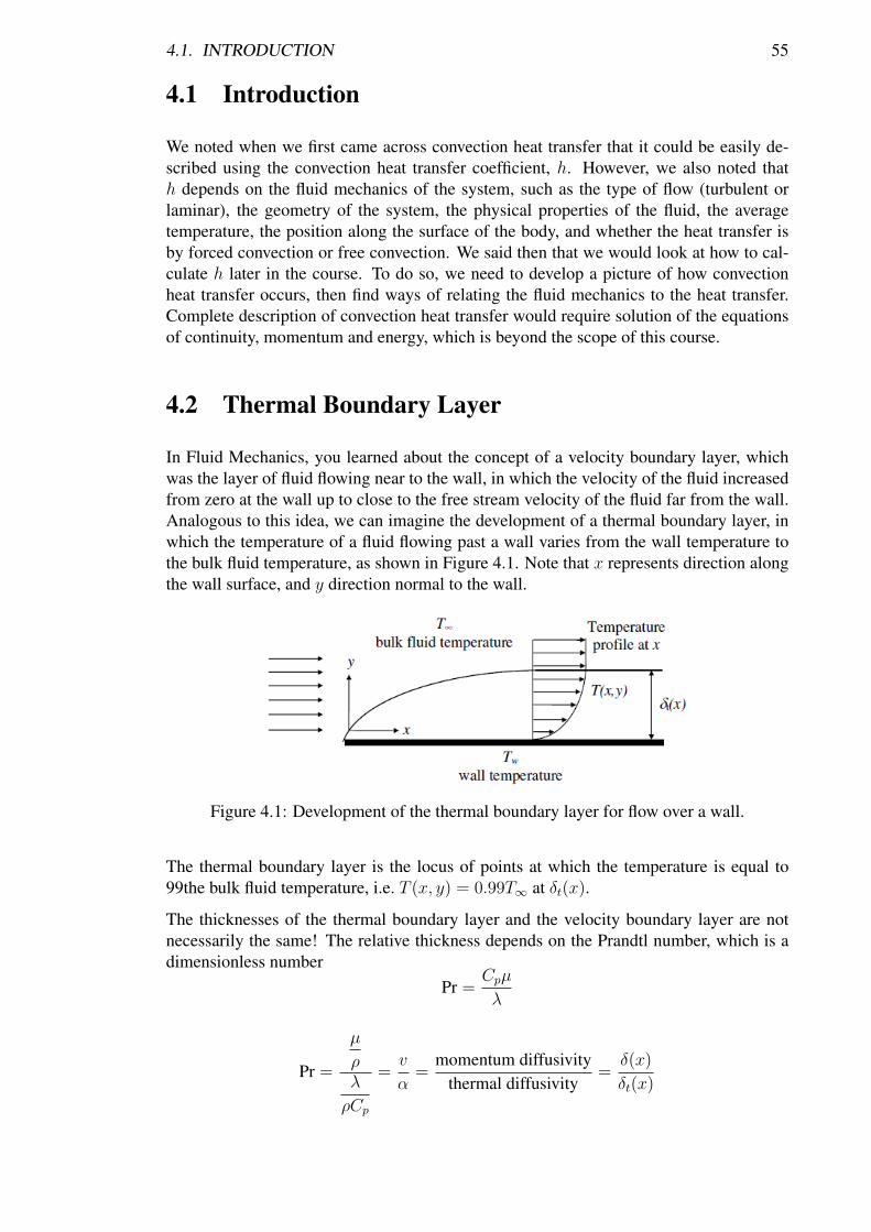
4.1. INTRODUCTION 55
4.1 Introduction
We noted when we first came across convection heat transfer that it could be easily de-scribed using the convection heat transfer coefficient, h. However, we also noted thath depends on the fluid mechanics of the system, such as the type of flow (turbulent orlaminar), the geometry of the system, the physical properties of the fluid, the averagetemperature, the position along the surface of the body, and whether the heat transfer isby forced convection or free convection. We said then that we would look at how to cal-culate h later in the course. To do so, we need to develop a picture of how convectionheat transfer occurs, then find ways of relating the fluid mechanics to the heat transfer.Complete description of convection heat transfer would require solution of the equationsof continuity, momentum and energy, which is beyond the scope of this course.
4.2 Thermal Boundary Layer
In Fluid Mechanics, you learned about the concept of a velocity boundary layer, whichwas the layer of fluid flowing near to the wall, in which the velocity of the fluid increasedfrom zero at the wall up to close to the free stream velocity of the fluid far from the wall.Analogous to this idea, we can imagine the development of a thermal boundary layer, inwhich the temperature of a fluid flowing past a wall varies from the wall temperature tothe bulk fluid temperature, as shown in Figure 4.1. Note that x represents direction alongthe wall surface, and y direction normal to the wall.
Figure 4.1: Development of the thermal boundary layer for flow over a wall.
The thermal boundary layer is the locus of points at which the temperature is equal to99the bulk fluid temperature, i.e. T (x, y) = 0.99T∞ at δt(x).
The thicknesses of the thermal boundary layer and the velocity boundary layer are notnecessarily the same! The relative thickness depends on the Prandtl number, which is adimensionless number
Pr =Cpµ
λ
Pr =
µ
ρλ
ρCp
=v
α=
momentum diffusivitythermal diffusivity
=δ(x)
δt(x)

56 CHAPTER 4. HEAT TRANSFER BY CONVECTION
The Prandtl number is a measure of the ratio of momentum diffusivity to heat diffusivity.If this ratio is equal to unity, as it is for gases, then the thermal and velocity boundarylayers have the same thickness, i.e.
δ(x) = δt(x) for Pr = 1 (gases)
For fluids for which Pr � 1, such as liquid metals, the thermal boundary layer is muchthicker than the velocity boundary layer i.e. heat is propagated through the fluid to agreater extent than momentum. For fluids for which Pr� 1, such as ordinary liquids andoils, the thermal boundary layer is much thinner than the velocity boundary layer.
4.3 Relating Convection Heat Transfer to Fluid Mechan-ics using Dimensionless Numbers
Suppose the temperature distribution, T (x, y), in the thermal boundary layer were known.Then the heat flux from the fluid to the wall at the point x along the wall would be givenby
q (x) = λf∂ T (x, y)
∂ y
∣∣∣∣y=0
where λf is the thermal conductivity of the fluid. (Note we are omitting the negative signfor convenience.) But we don’t generally know the temperature distribution, so insteadwe define a local heat transfer coefficient h(x) such that the heat flux between the fluidand the wall at point x along the surface of the wall is given by
q (x) = h (x) (T∞ − Tw)
Note that the local heat transfer coefficient can vary along the wall i.e. h(x) is a functionof x. Equating the above two equations gives
h (x) = λf
∂ T
∂ y
∣∣∣∣y=0
T∞ − Tw
Let us now define a dimensionless temperature θ(x, y) as
θ (x, y) =T (x, y)− TwT∞ − Tw
Clearly, θ(x, y) will vary from 0 at the wall to 1 in the bulk fluid. We can then write theabove equation in terms of this dimensionless temperature as
h (x) = λf∂ θ (x, y)
∂ y
∣∣∣∣y=0

4.4. LAMINAR FLOW ALONG A FLAT PLATE 57
4.4 Laminar Flow along a Flat Plate
An approximate expression for the temperature profile in the thermal layer for laminarflow along a flat plate is given by
θ (x, y) =3
2
y
δt (x)− 1
2
[y
δt (x)
]3
Similarly, an expression for the thickness of the thermal boundary layer is given by
δt (x) = 4.53x
Re0.5x Pr0.333
where the local Reynolds number, Rex is defined as
Rex =u∞x
v
where u∞ is the bulk fluid velocity, v is the kinematic viscosity (µ/ρ), and x is the distancealong the plate.
The heat transfer coefficient is related to the temperature profile by
h (x) = λf∂ θ (x, y)
∂ y
∣∣∣∣y=0
∂ θ (x, y)
∂ y
∣∣∣∣y=0
=3
2δt (x)
Thereforeh (x) =
3λf2δt (x)
Substituting in our expression for δt(x) gives
h (x) =3λfRe0.5
x Pr0.333
2× 4.53× x
= 0.331λfx
Re0.5x Pr0.333
Rearranging to give three dimensionless groups gives
Nux =h (x)x
λf= 0.331Re0.5
x Pr0.333
where Nux is the local Nusselt number, and is a function of the Prandtl and Reynoldsnumbers. Note that h(x) varies with x−0.5, i.e. the convection heat transfer coefficientalong the length of the wall decreases, as we noted earlier.
In fact, the exact expression for laminar flow along a flat plate is given by
Nux =h (x)x
λf= 0.332Re0.5
x Pr0.333
58 CHAPTER 4. HEAT TRANSFER BY CONVECTION
so our analysis is pretty close. The range of application for this correlation is Rex <5× 10⁵, 0.6 < Pr < 10, and it applies when the wall temperature of the plate is constantalong the plate.
The above example introduces the Nusselt number, which is an important dimensionlessgroup for describing convection heat transfer. Looking closely at the general form of theNusselt number, using a characteristic dimension L, it is clearly a ratio of
Nu =hL
λf=
h∆T
λfL
∆T
which can be interpreted as the ratio of convection heat transfer to conduction heat transferacross the thermal boundary layer.
The example also demonstrates that the Nusselt number is a function of the Reynoldsand Prandtl numbers, which describe the fluid mechanics of the system. This sort ofexpression therefore gives us our goal, which was to relate the convection heat transfercoefficient to the fluid mechanics. Knowing the fluid mechanics, we can calculate Re andPr, and from these predict the convection heat transfer coefficient. Similar expressionshave been developed for other systems e.g. flow in tubes, along ducts, turbulent flow etc.Clearly in these cases the temperature profile and thermal boundary layer profile will bedifferent, so the equations will be different, but they often have this general form. In thenext lecture we will look at some of these.
4.5 Correlations for Predicting the Convection Heat Trans-fer Coefficient
4.5.1 Forced Convection, Fully Developed Turbulent Flow in Smooth,Circular Pipes
One correlation (among many!) for forced convection fully developed turbulent flowinside smooth tubes is given by the Sieder and Tate equation:
Nu = 0.027Re0.8Pr0.333
(µbµw
)0.14
This equation is applicable for the following range of conditions:
• 0.7 < Pr < 16, 700
• Re > 10, 000 (Re = umD/v)
• L/D > 60
• smooth pipes
The term (µb/µw)0.14 is a correction factor which accounts for the fact that the fluid vis-cosity changes with temperature near the wall.
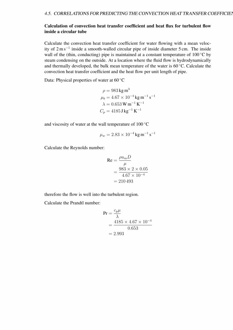
4.5. CORRELATIONS FOR PREDICTING THE CONVECTION HEAT TRANSFER COEFFICIENT59
Calculation of convection heat transfer coefficient and heat flux for turbulent flowinside a circular tube
Calculate the convection heat transfer coefficient for water flowing with a mean veloc-ity of 2 m s−1 inside a smooth-walled circular pipe of inside diameter 5 cm. The insidewall of the (thin, conducting) pipe is maintained at a constant temperature of 100 ◦C bysteam condensing on the outside. At a location where the fluid flow is hydrodynamicallyand thermally developed, the bulk mean temperature of the water is 60 ◦C. Calculate theconvection heat transfer coefficient and the heat flow per unit length of pipe.
Data: Physical properties of water at 60 ◦C
ρ = 983 kg m3
µb = 4.67× 10⁻⁴ kg m−1 s−1
λ = 0.653 W m−1 K−1
Cp = 4185 J kg−1 K−1
and viscosity of water at the wall temperature of 100 ◦C
µw = 2.83× 10⁻⁴ kg m−1 s−1
Calculate the Reynolds number:
Re =ρumD
µ
=983× 2× 0.05
4.67× 10−4
= 210 493
therefore the flow is well into the turbulent region.
Calculate the Prandtl number:
Pr =cpµ
λ
=4185× 4.67× 10−4
0.653= 2.993

60 CHAPTER 4. HEAT TRANSFER BY CONVECTION
Then
Nu = 0.027Re0.8Pr0.333
(µbµw
)0.14
= 0.027× 210 4930.8 × 2.9930.333 ×(
4.67
2.83
)0.14
= 0.027× 18 138× 1.441× 1.073
= 757.2
hD
λ= 757.2
h =757.2× 0.653
0.05= 9889 W m−2 K−1
q = h (Tw − Tf )= 9889× (100− 60)
= 395 597 W m−2
The area per meter of pipe is,
A = πDh
= π × 0.05× 1
= 0.1571 m2 m−1
Q = qA
= 395 567× 0.1571
= 62 112 W m−1
The above example demonstrates the use of a convection heat transfer correlation. Thereare many such correlations, developed for different geometrical situations e.g. pipes,ducts, flat plates, and applicable over different ranges of conditions e.g. laminar or tur-bulent flow, range of Prandtl number. The important thing is to know that, to use a cor-relation, you must be sure that it is applicable to your particular system, and that youare operating within its range of applicability. You should also bear in mind that theiraccuracy is perhaps only ±25%.
4.5.2 Forced Convection, Laminar Flow over a flat Plate
Local Nusselt number, Nux,
Nux = 0.332Re0.5x Pr0.333
Average Nusselt number, Num, over a distance L
Num = 0.664Re0.5L Pr0.333
Range of application: ReL < 5× 10⁵, 0.6 < Pr < 10, constant wall temperature.
4.5. CORRELATIONS FOR PREDICTING THE CONVECTION HEAT TRANSFER COEFFICIENT61
4.5.3 Forced Convection, Turbulent Flow over a Flat Plate
Local Nusselt number, Nux,
Nux = 0.029Re0.8x Pr0.43
Average Nusselt number, Num, over a distance L
Num = 0.036(Re0.8
L − 9200)
Pr0.43
(µbµw
)0.25
Range of application: 2× 10⁵ < ReL < 5.5× 10⁶, 0.7 < Pr < 380, 0.26 < µb/µw < 3.5,constant wall temperature.
4.5.4 Forced Convection, Fully Developed Laminar Flow in Smooth,circular Pipes
Nu = 4.364
Range of application: Re < 2300, constant wall heat flux along the pipe.
Nu = 3.66
Range of application: Re < 2300, constant wall temperature along the pipe.
4.5.5 Forced Convection, Entrance Region of a Circular Tube
Num = 3.66 +0.0668Gz
1 + 0.04Gz0.667
where Gz = Re Pr/ (L/D) = Graetz number and L is distance from inlet.
Range of application: Gz < 100, constant wall temperature
4.5.6 Forced Convection, Fully Developed Turbulent Flow in Smooth,Circular Pipes
Colburn Equation
Nu = 0.023Re0.8Pr0.333
Range of application: 0.7 < Pr < 160, Re > 10 000, L/D > 60, smooth pipes.
Dittus-Boelter Equation
Nu = 0.023Re0.8Prn
where n = 0.4 for heating and 0.3 for cooling.
Range of application: 0.7 < Pr < 160, Re > 10 000, L/D > 60, smooth pipes.
62 CHAPTER 4. HEAT TRANSFER BY CONVECTION
Sieder and Tate Equation
Nu = 0.027Re0.8Pr0.333
(µbµw
)0.14
Range of application: 0.7 < Pr < 16 700, Re > 10 000, L/D > 60, smooth pipes.
Petukhov Equation
Nu =Re Pr
1.07 + 12.7(Pr0.667 − 1
)(f8
)0.5
(f
8
)(µbµw
)n
where
n = 0.11 for heating with uniform Tw
= 0.25 for cooling with uniform Tw
= 0.0 for uniform wall heat flux or for gases
and f is the friction factor.
Range of application: 104 < Re < 5× 10⁶, 0.5 < Pr < 200 with 5-6% error, 0.5 < Pr <2000 with 10% error, 0.025 < µb/µw < 12.5.
For non-circular ducts, the tube diameter in the above correlations can be replaced by thehydraulic diameter, Dh, of the non-circular duct, defined as
Dh =4AcP
where Ac is the cross sectional area and P is the wetted perimeter.
4.6. PROBLEMS 63
4.6 Problems
1. A refrigerated lorry container is being designed. The container of the lorry is 7 mlong, 3 m high and 2 m wide. A worst case scenario is assumed, that the lorry istravelling at 60 miles per hour on a hot sunny day with the ambient air temperatureat 30 ◦C.
(a) Calculate the rate of convective heat transfer to the top and two sides of thelorry container, if their surfaces are at 18 ◦C. (Ignore the lorry’s cab, under-side and back doors.) Use the following correlation to calculate the averageconvection heat transfer coeffcient for air flowing over a flat surface of lengthL:
h =λ
L
(0.0125Re0.8
L − 287)
Use the following physical properties of air at 30 ◦C: λ = 0.026 W m−1 K−1,ρ = 1.163 kg m−3, µ = 1.86× 10⁻⁵ Pa s.
(b) Solar radiation falls onto the top and one side of the lorry at a flux of 500 W m−2.Calculate the total cooling duty required to maintain the container’s steadystate internal temperature.
(c) The walls of the container are made of insulation (thermal conductivity of0.11 W m−1 K−1) sandwiched between two stainless steel sheets, each of 5 mmthickness and with a thermal conductivity of 19 W m−1 K−1.
(d) If the outer surface of the lorry walls are at 18 ◦C, and the inside wall of thechamber is to be maintained at 2 ◦C, calculate the thickness of the insulationrequired. Assume heat enters the lorry container only through the top and twosides (ignore the front, back and underside).
2. Energy is generated at a constant rate of 104 W m−3 throughout a slab of thickness10 cm and constant thermal conductivity 1.2 W m−1 K−1. The boundary surfaceon one side is insulated so that there is no heat flow across this boundary, andon the other dissipates heat by convection into a fluid at temperature 20 ◦C with aheat transfer coefficient 74 W m−2 K−1. Calculate the steady state temperature atboth surfaces of the slab, and the heat flux from the slab into the fluid. Sketch thetemperature profile and heat flux profile through the slab. (N.B. The heat flux canbe calculated in three ways - from the temperature profile at the slab surface, fromthe convection heat transfer equation, and one other way - what is it?)
[T (0) = 75.18 ◦C, T (L) = 33.51 ◦C, Q = 1000 W m−2]
3. A wall of thickness L and constant thermal conductivity λ is irradiated with gammarays at the surface x = 0. The gamma rays attenuate as they pass through the wall,and in so doing convert their energy into heat. This volumetric heat generationvaries through the wall at a rate given by G(x) = G0 exp (−βx) where G0 andβ are constants. The boundary surface at x = 0 is kept thermally insulated, andthe boundary surface at x = L dissipates heat by convection with convection heattransfer coefficient h into a fluid at temperature Tf . Develop an expression for thesteady state heat flux throughout the wall as a function of distance x, and for thewall surface temperature at x = L.
[q =G0
β(1− exp (−βx)), T (L) = Tf +
G0
hβ(1− exp (−βL))]
64 CHAPTER 4. HEAT TRANSFER BY CONVECTION
4. For the system described in the question above, calculate the convection heat fluxand the wall surface temperature at x = L, for G0 = 104 W m−3, β = 3 m−1,L = 0.5 m, λ = 2.5 W m−1 K−1, h = 70 W m−2 K−1, Tf = 15 ◦C.
5. A wire of radius R and constant thermal conductivity λ carrying current generatesheat at a constant rate throughout of gW m−3. The heat is dissipated by convectioninto the ambient air at a temperature Tf with a heat transfer coefficient h.
(a) Show that the expression for the steady state temperature profile throughoutthe wire is given by
T (r) =g
4λR2
(1−
( rR
)2)
+gR
2h+ Tf
(b) Derive an expression for the heat flux profile throughout the wire. Sketch thetemperature profile and heat flux profile.
(c) For the above wire and the following data: g = 6× 10⁶ W m−3, R = 1.5 mm,Tf = 10 ◦C, λ = 2.5 W m−1 K−1, h = 45 W m−2 K−1; calculate the tempera-ture at the surface of the wire.
Chapter 5Applications of Heat Transfer in ChemicalEngineering
Contents5.1 Introduction . . . . . . . . . . . . . . . . . . . . . . . . . . . . . . . 67
5.2 Heat Loss through Composite Cylinders . . . . . . . . . . . . . . . . 67
5.2.1 Critical Thickness of Insulation, and the Paradox of cylindricalInsulation . . . . . . . . . . . . . . . . . . . . . . . . . . . . . 69
5.3 Transient Heating and Cooling of Mixing Vessels and of Solids ofHigh λ . . . . . . . . . . . . . . . . . . . . . . . . . . . . . . . . . . . 71
5.3.1 Example . . . . . . . . . . . . . . . . . . . . . . . . . . . . . 73
5.4 Problems . . . . . . . . . . . . . . . . . . . . . . . . . . . . . . . . . 75
65

66

5.1. INTRODUCTION 67
5.1 Introduction
We started this course by stating that heat transfer is one of the most useful things youwill ever learn, for several reasons, including that many processing situations involve heattransfer, and that it is an excellent example of transport phenomena. Next year you will doa course called Momentum, Heat and Mass Transfer, which will aim to bring these threetopics together and show that, mathematically, they have the same form. That course willthen concentrate on the mathematics, so that you become competent at solving problemsfor any of the three transport phenomena. But you will cope with that course much betterif you have a good grasp of the physical situations that all this maths describes. Thatis why, throughout this course, we have tried to highlight what is happening physically,recognising that the maths is simply a tool to describe the physical situation quantitatively.(Show an overhead from Momentum, Heat and Mass Transfer.)
But the other, more immediately practical reason that heat transfer will be so useful toyou is that it applies to many processing situations of practical interest. So for the restof this course, we are going to apply the heat transfer principles that you have learned totypical industrial problems.
One such problem is heat losses from insulated pipes carrying hot fluids. We know thatfor steady state heat transfer through a composite slab, we simply add the resistances toheat transfer, both for conduction through the slab, and for convection at the surface. Theresistance to heat transfer for conduction through a slab is given by R = 1/UA = x/Al,and for convection is given by R = 1/hA. But with cylinders and spheres, the areaincreases with radius, so the expression for the thermal resistance is more complicated,and had to be derived by solving Laplace’s equation, as we did in Lecture 10. Today wewill apply this to heat loss through composite cylinders, in particular, insulated pipes, andwe will learn why sometimes adding insulation to pipes is counter-productive, as it canactually increase heat loss.
5.2 Heat Loss through Composite Cylinders
As noted earlier, cylindrical systems are of great interest to process engineers, as pipes arecylindrical, and much of a process plant is taken up with pipework. Often these pipes arecarrying hot fluids, such as steam, and often they are insulated to minimise heat losses.It is important that we are able to calculate the amount of insulation required, and thatrequires us to be able to calculate the heat loss across composite coaxial cylinders i.e.several cylindrical layers in series, as shown in Figure 5.1.
The clearest way to approach this is to utilise the thermal resistance concept introducedearlier, that the resistance to heat flow is determined by summing the individual resis-tances across each layer, along with the convection heat transfer resistances on the insideand outside of the pipe. This will only work for steady state conditions, as the thermalresistance analogy only applies for steady state.
Q =Ta − TbR
=Ta − Tb
Ra +R1 +R2 +Rb

68CHAPTER 5. APPLICATIONS OF HEAT TRANSFER IN CHEMICAL ENGINEERING
Figure 5.1: Radial heat flow through a hollow composite cylinder with layers in perfectthermal contact.
For convection heat transfer, we know that the resistance to heat transfer is given by
R =1
hA
Therefore
Ra =1
ha2πr0H
Rb =1
hb2πr2H
We have previously derived the temperature profile and heat flux across a cylindrical wall,and found that the resistance to heat transfer was given by
R =
ln
(rori
)2πHλ
Therefore, for each of the two layers in the composite cylinder,
R1 =
ln
(r1
r0
)2πHλ1
R2 =
ln
(r2
r1
)2πHλ2
We can thus calculate each of the resistances, add them together, and divide the tempera-ture difference by the sum to get the heat flow rate.
R =1
UA=
1
ha2πr0H+
ln
(r1
r0
)2πHλ1
+
ln
(r2
r1
)2πHλ2
+1
hb2πr2H

5.2. HEAT LOSS THROUGH COMPOSITE CYLINDERS 69
In calculations, the overall heat transfer coefficient is usually based on the outer tubesurface, in this case, r2. The overall heat transfer coefficient can be defined as
UoAo =1
1
ha2πr0H+
ln
(r1
r0
)2πHλ1
+
ln
(r2
r1
)2πHλ2
+1
hb2πr2H
Uo =
[Ao
(1
ha2πr0H+
1
2πHλ1
ln
(r1
r0
)+
1
2πHλ2
ln
(r2
r1
)+
1
hb2πr2H
)]−1
=
(2πr2H
ha2πr0H+
2πr2H
2πHλ1
ln
(r1
r0
)+
2πr2H
2πHλ2
ln
(r2
r1
)+
2πr2H
hb2πr2H
)−1
=
(r2
har0
+r2
λ1
ln
(r1
r0
)+r2
λ2
ln
(r2
r1
)+
1
hb
)−1
Or often in terms of the diameters,
Uo =
[D2
D0
1
ha+D2
2λ1
ln
(D1
D0
)+D2
2λ2
ln
(D2
D1
)+
1
hb
]−1
5.2.1 Critical Thickness of Insulation, and the Paradox of cylindricalInsulation
Now, consider what happens when we add a layer of insulation to a cylindrical pipe. Theresistance to heat transfer contributed by the insulation is given by
Rins =
ln
(r2
r1
)2πHλins
Clearly as r2 increases (and r1 stays constant), the resistance to heat transfer increases,which is what you would expect.
Consider also the resistance to convection heat transfer at the surface, given by
Rb =1
hb2πr2H
Here, as r2 increases, the resistance to heat transfer actually decreases, as the area for heattransfer increases.
So as we add insulation to a pipe, the resistance to conduction heat transfer through theinsulation increases, but the resistance to convection heat transfer at the surface decreases.At some point, there will be a minimum resistance, which would correspond to a maxi-mum heat loss. So the paradox of cylindrical insulation is that, it is possible, by addinginsulation to a pipe, to actually increase the heat loss!
It is important, therefore, to know at what thickness of insulation you are actually increas-ing heat loss, so that you can be sure that you put on a greater thickness than this. But insome situations, we can actually use this to our advantage, for example when we want tomaximise heat loss to avoid overheating. So electric wires and power cables often have acoating of just the right thickness to maximise cooling.
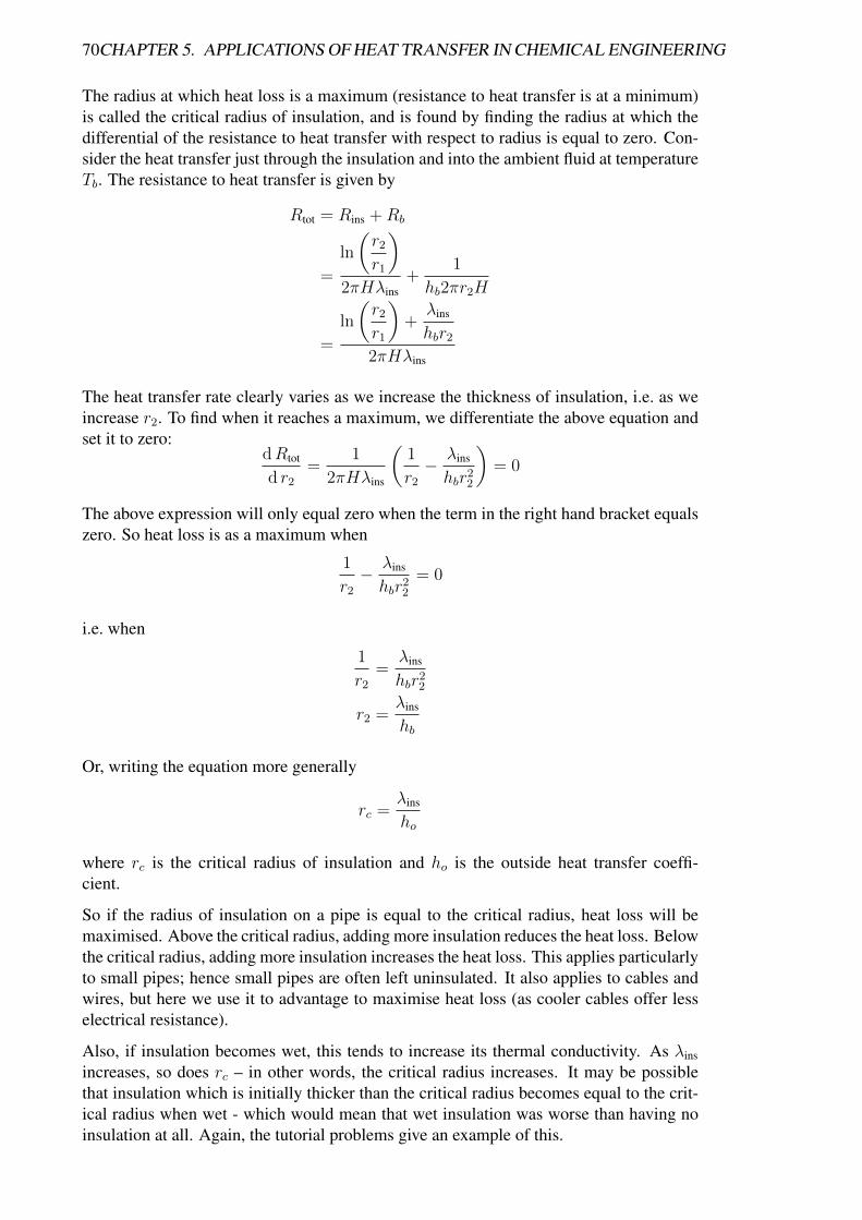
70CHAPTER 5. APPLICATIONS OF HEAT TRANSFER IN CHEMICAL ENGINEERING
The radius at which heat loss is a maximum (resistance to heat transfer is at a minimum)is called the critical radius of insulation, and is found by finding the radius at which thedifferential of the resistance to heat transfer with respect to radius is equal to zero. Con-sider the heat transfer just through the insulation and into the ambient fluid at temperatureTb. The resistance to heat transfer is given by
Rtot = Rins +Rb
=
ln
(r2
r1
)2πHλins
+1
hb2πr2H
=
ln
(r2
r1
)+λins
hbr2
2πHλins
The heat transfer rate clearly varies as we increase the thickness of insulation, i.e. as weincrease r2. To find when it reaches a maximum, we differentiate the above equation andset it to zero:
dRtot
d r2
=1
2πHλins
(1
r2
− λins
hbr22
)= 0
The above expression will only equal zero when the term in the right hand bracket equalszero. So heat loss is as a maximum when
1
r2
− λins
hbr22
= 0
i.e. when
1
r2
=λins
hbr22
r2 =λins
hb
Or, writing the equation more generally
rc =λins
ho
where rc is the critical radius of insulation and ho is the outside heat transfer coeffi-cient.
So if the radius of insulation on a pipe is equal to the critical radius, heat loss will bemaximised. Above the critical radius, adding more insulation reduces the heat loss. Belowthe critical radius, adding more insulation increases the heat loss. This applies particularlyto small pipes; hence small pipes are often left uninsulated. It also applies to cables andwires, but here we use it to advantage to maximise heat loss (as cooler cables offer lesselectrical resistance).
Also, if insulation becomes wet, this tends to increase its thermal conductivity. As λins
increases, so does rc – in other words, the critical radius increases. It may be possiblethat insulation which is initially thicker than the critical radius becomes equal to the crit-ical radius when wet - which would mean that wet insulation was worse than having noinsulation at all. Again, the tutorial problems give an example of this.
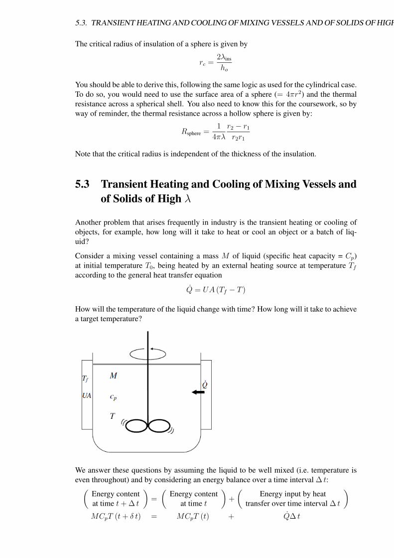
5.3. TRANSIENT HEATING AND COOLING OF MIXING VESSELS AND OF SOLIDS OF HIGH λ71
The critical radius of insulation of a sphere is given by
rc =2λins
ho
You should be able to derive this, following the same logic as used for the cylindrical case.To do so, you would need to use the surface area of a sphere (= 4πr2) and the thermalresistance across a spherical shell. You also need to know this for the coursework, so byway of reminder, the thermal resistance across a hollow sphere is given by:
Rsphere =1
4πλ
r2 − r1
r2r1
Note that the critical radius is independent of the thickness of the insulation.
5.3 Transient Heating and Cooling of Mixing Vessels andof Solids of High λ
Another problem that arises frequently in industry is the transient heating or cooling ofobjects, for example, how long will it take to heat or cool an object or a batch of liq-uid?
Consider a mixing vessel containing a mass M of liquid (specific heat capacity = Cp)at initial temperature T0, being heated by an external heating source at temperature Tfaccording to the general heat transfer equation
Q = UA (Tf − T )
How will the temperature of the liquid change with time? How long will it take to achievea target temperature?
We answer these questions by assuming the liquid to be well mixed (i.e. temperature iseven throughout) and by considering an energy balance over a time interval ∆ t:(
Energy contentat time t+ ∆ t
)=
(Energy content
at time t
)+
(Energy input by heat
transfer over time interval ∆ t
)MCpT (t+ δ t) = MCpT (t) + Q∆ t

72CHAPTER 5. APPLICATIONS OF HEAT TRANSFER IN CHEMICAL ENGINEERING
Rearranging
Q =MCp (T (t+ ∆ t)− T (t))
∆ t= MCp
(T (t+ ∆ t)− T (t))
∆ t
As ∆ t goes to zero, the right hand side becomes the differential of T with respect to time.Also, substituting in for Q gives
Q = UA (Tf − T ) = MCpdT
d t
in other words, the rate of heat transfer at any moment is balanced by the rate of change oftemperature. To find an explicit expression for temperature at time t, we need to rearrangeand integrate:
dT
Tf − T=
UA
MCpd t∫ T (t)
T0
dT
Tf − T=
∫ t
0
UA
MCpd t
[− ln (Tf − T )]T (T )T0
=UA
MCpt
− ln
(Tf − T (t)
Tf − T0
)=
UA
MCpt
Tf − T (t)
Tf − T0
= exp
[− UA
MCpt
]= exp
[− tτ
]where τ = MCp/UA is the time constant for the system.
Note that the left hand side expression is a dimensionless temperature expression whichvaries from 1 initially to zero after an infinitely long time. So the temperature of thevessel contents approaches the heating temperature by exponential decay. The analysisapplies whether we are heating or cooling, provided the heat source maintains a constanttemperature.
The above analysis would apply, for example, to a steam jacketed vessel, in which thesteam temperature stays constant throughout the heating process. Note that we could heatthe vessel contents in other ways, for example, by direct steam injection (which wouldalter the mass of the liquid as it heated), or by direct electrical heating (in which caseheat transfer would be at a constant rate and the temperature would increase linearly withtime), or by a heating fluid which is simultaneously cooling so that its temperature is alsochanging.
The above analysis also applies to heating (or cooling) of a solid of very high thermal con-ductivity (so that the temperature throughout can be considered uniform, equivalent to theassumption above that the liquid is well mixed). This type of analysis is called a lumpedsystem analysis. We can determine whether a lumped system analysis is appropriate for asolid, i.e. whether the temperature distribution in the solid is sufficiently uniform for thissort of analysis, by defining a dimensionless number called the Biot number, Bi, as
Bi =hLsλs
5.3. TRANSIENT HEATING AND COOLING OF MIXING VESSELS AND OF SOLIDS OF HIGH λ73
where λs is the thermal conductivity of the solid and Ls is the characteristic length, givenby
Ls =V
A
i.e. volume divided by surface area for heat transfer. For a sphere, the characteristic lengthis
Ls =
4
3πr3
4πr2=r
3=D
6
and for a slab heated on both sides it is half the thickness of the slab, L/2.
The lumped system analysis will then be accurate within about 5% if Bi < 0.1.
The physical significance of the Biot number becomes clearer if it is written as
Bi =h
λsLs
where it is clearly the ratio of heat transfer by convection to the solid to heat transfer byconduction within the solid. So, if heat transfer within the solid is very fast, the tempera-ture within the solid will be fairly uniform, and the Biot number will be small.
The analysis also applies to a fluid flowing along a pipe, in which case time can be re-placed by distance down the pipe, resulting in
Tf − T (x)
Tf − T0
= exp
[− UA
MCpx
]= exp
[− xX
]
where X = MCp/UA with units of m, where A is the surface area for heat transfer permeter of pipe.
5.3.1 Example
An aluminium plate (λ = 160 W m−1 K−1, ρ = 2790 kg m−3, Cp = 880 J kg−1 K−1) ofthickness L = 3 cm and at a uniform intial temperature of 225 ◦C is suddenly immersedinto a well-stirred fluid maintained at a constant temperature of 25 ◦C. The heat transfercoefficient between the plate and the fluid is 320 W m−2 K−1. Determine the time requiredfor the centre of the plate to cool to 50 ◦C.
A lumped system analysis is appropriate if Bi < 0.1. The characteristic dimension isgiven by
Ls =Volume
Area=LA
2A=L
2= 1.5 cm
Therefore
Bi =hLsλs
=320× 1.5× 10−2
160= 3× 10⁻²
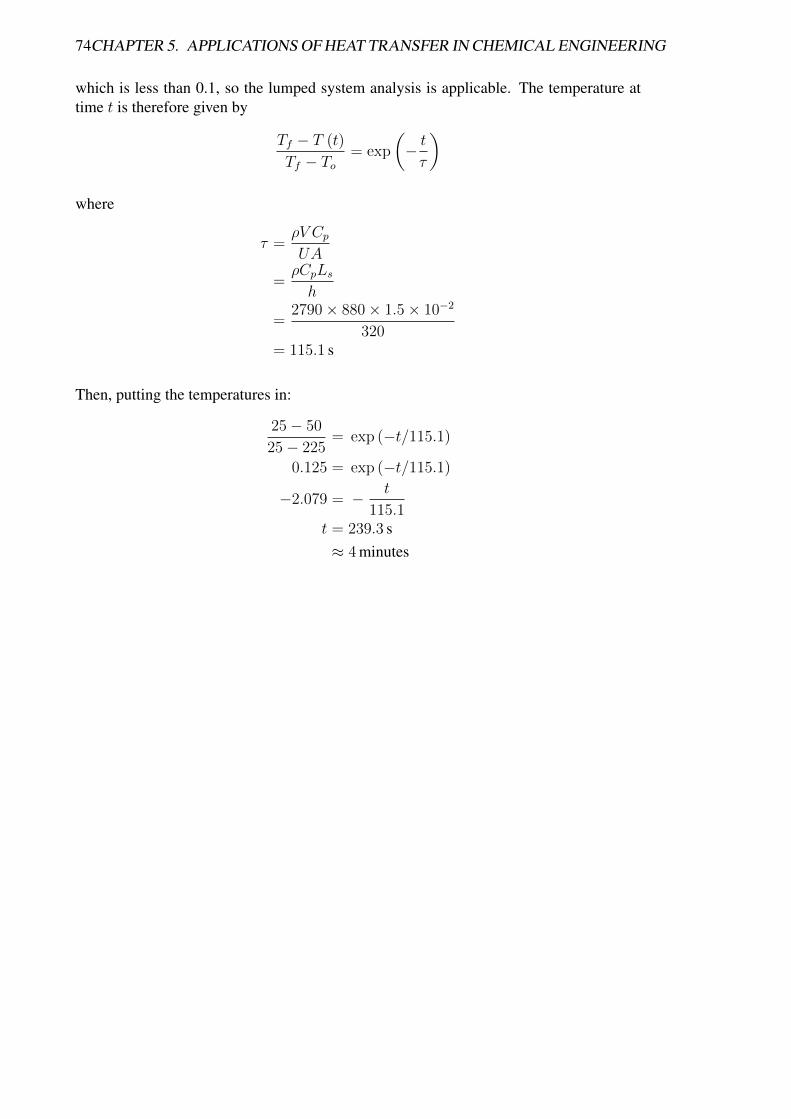
74CHAPTER 5. APPLICATIONS OF HEAT TRANSFER IN CHEMICAL ENGINEERING
which is less than 0.1, so the lumped system analysis is applicable. The temperature attime t is therefore given by
Tf − T (t)
Tf − To= exp
(− tτ
)
where
τ =ρV CpUA
=ρCpLsh
=2790× 880× 1.5× 10−2
320= 115.1 s
Then, putting the temperatures in:
25− 50
25− 225= exp (−t/115.1)
0.125 = exp (−t/115.1)
−2.079 = − t
115.1t = 239.3 s≈ 4 minutes

5.4. PROBLEMS 75
5.4 Problems
1. The contents of a jacketed fermentation vessel with a capacity of 30 m3 of liquidare to be heated using steam condensing in the jacket at 121 ◦C. The heat trans-fer area of the jacketed vessel is 25 m2, and the overall heat transfer coefficient is1500 W m−2 K−1. The density of the fermentation broth is 1020 kg m−3, its specificheat capacity is 3880 J kg−1 K−1, and the broth is well mixed. The initial tempera-ture of the broth is 15 ◦C. Ignoring the thermal resistance and heat capacity of thevessel walls, calculate the time (in minutes) required to raise the temperature of thebroth to 100 ◦C.
[85 minutes]
2. After allowing for the heat generated by respiration, a fermenter loses heat at a rateof 8 kW, which must be replaced to maintain the temperature in the fermenter at37 ◦C. This heat duty is to be supplied by a thin helical copper coil of internal diam-eter 1.5 cm passing through the fermenter, carrying hot water at 90 ◦C. The averagevelocity of water in the tube is 1.8 m s−1. Calculate the heat transfer coefficient inthe tube using the Seider and Tate correlation
Nu = 0.027Re0.8Pr0.333
(µbµw
)0.14
If the heat transfer coefficient on the outside of the tube is 1500 W m−2 K−1, cal-culate the overall heat transfer coefficient, heat flow rate per unit length of pipe,and the length of pipe required to achieve the required heat transfer duty. Ignorethe thickness and thermal resistance of the copper pipe, and assume the pipe walltemperature to be 70 ◦C.
Thermophysical properties of water at 90 ◦C,
λ = 0.676 W m−1 K−1
ρ = 965 kg m−3
µ = 316× 10−6 Pa sCp = 4207 J kg−2 K−1
and viscosity of water at 70 ◦C = 405× 10−6 Pa s
[12 622 W m−2 K−1, 1341 W m−2 K−1, 3349 W, 2.39 m]
3. (a) Explain why the steady state rate of heat transfer through several layers in se-ries is the same through each layer, even if their thermal conductivities differ,and how this is achieved.
(b) A cylindrical fermenter is to be maintained at 37 ◦C. The fermenter is 4 mtall and 1.5 m in diameter, and is made of 5 mm thick stainless steel (λ =19 W m−1 K−1).
Calculate the steady state rate of heat loss to the surrounding air at 10 ◦C, ifthe liquid side heat transfer coefficient is 150 W m−2 K−1 and the air side heattransfer coefficient is 10 W m−2 K−1. Assume the fermenter is full of liquid,and that heat loss occurs through the sides, top and bottom.
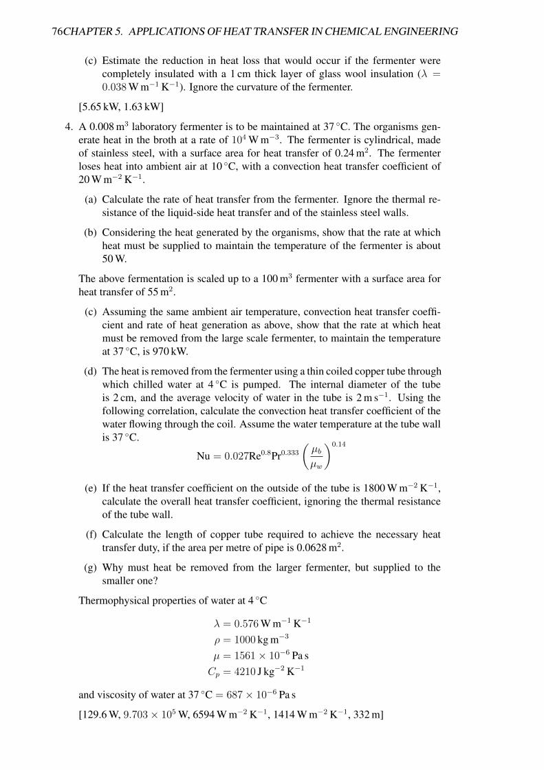
76CHAPTER 5. APPLICATIONS OF HEAT TRANSFER IN CHEMICAL ENGINEERING
(c) Estimate the reduction in heat loss that would occur if the fermenter werecompletely insulated with a 1 cm thick layer of glass wool insulation (λ =0.038 W m−1 K−1). Ignore the curvature of the fermenter.
[5.65 kW, 1.63 kW]
4. A 0.008 m3 laboratory fermenter is to be maintained at 37 ◦C. The organisms gen-erate heat in the broth at a rate of 104 W m−3. The fermenter is cylindrical, madeof stainless steel, with a surface area for heat transfer of 0.24 m2. The fermenterloses heat into ambient air at 10 ◦C, with a convection heat transfer coefficient of20 W m−2 K−1.
(a) Calculate the rate of heat transfer from the fermenter. Ignore the thermal re-sistance of the liquid-side heat transfer and of the stainless steel walls.
(b) Considering the heat generated by the organisms, show that the rate at whichheat must be supplied to maintain the temperature of the fermenter is about50 W.
The above fermentation is scaled up to a 100 m3 fermenter with a surface area forheat transfer of 55 m2.
(c) Assuming the same ambient air temperature, convection heat transfer coeffi-cient and rate of heat generation as above, show that the rate at which heatmust be removed from the large scale fermenter, to maintain the temperatureat 37 ◦C, is 970 kW.
(d) The heat is removed from the fermenter using a thin coiled copper tube throughwhich chilled water at 4 ◦C is pumped. The internal diameter of the tubeis 2 cm, and the average velocity of water in the tube is 2 m s−1. Using thefollowing correlation, calculate the convection heat transfer coefficient of thewater flowing through the coil. Assume the water temperature at the tube wallis 37 ◦C.
Nu = 0.027Re0.8Pr0.333
(µbµw
)0.14
(e) If the heat transfer coefficient on the outside of the tube is 1800 W m−2 K−1,calculate the overall heat transfer coefficient, ignoring the thermal resistanceof the tube wall.
(f) Calculate the length of copper tube required to achieve the necessary heattransfer duty, if the area per metre of pipe is 0.0628 m2.
(g) Why must heat be removed from the larger fermenter, but supplied to thesmaller one?
Thermophysical properties of water at 4 ◦C
λ = 0.576 W m−1 K−1
ρ = 1000 kg m−3
µ = 1561× 10−6 Pa sCp = 4210 J kg−2 K−1
and viscosity of water at 37 ◦C = 687× 10−6 Pa s
[129.6 W, 9.703× 10⁵ W, 6594 W m−2 K−1, 1414 W m−2 K−1, 332 m]


![Energy transfer[1]](https://img.pdfslide.net/doc/110x75/58727eeb1a28abc7068b5dbf/energy-transfer1.jpg)