Embed Size (px)
Citation preview
Fluid - Structure and Soil - Structure Interaction of Bridge Piers
by W. Phillip Yen, Ph.D., P.E 1 and Kornel Kerenyi, Ph.D. 2
1 Research Structural Engineer, Seismic Hazard Mitigation (HRDI-07), Federal Highway Administration, 6300 Georgetown Pike, McLean, Virginia 22101; PH (202) 493-3056; FAX (202) 493-3442; email: [email protected] 2 Hydraulic Research Engineer, GKY and Associates, Inc., 5411-E Backlick Road, Springfield, Virginia 22151; PH (703) 642-5080; FAX (703) 642-5367; email: [email protected]
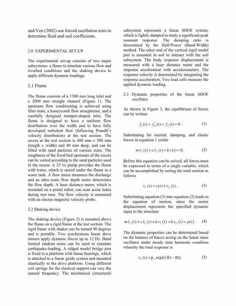
ABSTRACT The goal of this research is to test various combinations of hazards such as wind, flood, scour and dynamic loadings (e.g., earthquakes and vessel impacts) for impacts to bridge pier structural stability. Most equations and design criteria currently in use treat these hazards separately, although they can occur concurrently. A study that combines all hazards and dynamic loadings would be very complicated. Therefore the initial research is designed and fabricated to study only flow (flood), soil (sediment particle size and river bed geometry) and dynamic loading (harmonic, random and impulsive loads). A rigid mass, single degree of freedom (SDOF) oscillator represents the simplified bridge pier. A specially designed flume, which is 3000 mm long and 400 mm wide, allows for the investigation of different soil conditions and various flow velocities. The oscillating pier is mounted elastically on a structure over the test section of the flume. Two synchronous linear drive motors apply the dynamic loads. The oscillating bridge pier, neglecting flow and soil conditions, represents a perfect linear spring-damper system. In combination with flow and soil the system gets nonlinear. The goal of this initial research is to replace the soil and flow effects with an equivalent spring-damper system. This paper summarizes the fluid – structure interaction and the soil structure interaction tests. The equivalent spring and damping coefficients are plotted vs. forcing frequencies. KEYWORDS: multi hazard impacts on bridge piers, fluid structure interaction, soil structure
interaction 1.0 INTRODUCTION This study is concerned with the safety of bridges subjected to different natural hazard events. The events of interest are earthquakes, scour, hurricanes and vessel impact. Several bridge foundations are under water, so the structural response during an earthquake under these combined conditions is very complicated. Research at the Federal Highway Administration (FHWA) Turner Fairbanks Highway Research Center (TFHRC) Seismic Hazard Mitigation has focused on developing an experimental set-up to investigate a simple model where flow, scour (soil) and earthquakes (dynamic forces) interact with a bridge pier structure. The experimental set-up is designed to study the fluid-soil interaction of a rigid single degree of freedom (SDOF) oscillator using a forced oscillation experiment. The linear SDOF oscillator acts as a reference system to investigate the nonlinear behavior of the system when it interacts with fluid and soil. The identification procedure to determine the additional fluid and soil forces based on a forced oscillation test are similar used to identify fluid dynamic damping and stiffness. Staubli (1983) and Deniz (1997) used forced oscillation tests in a tow-tank to determine force coefficients and phase angle to describe the fluid dynamic system. Scruton (1963) and Bardowicks (1976) proposed a description of flow-induced load in the form of components in phase with body displacement and velocity. They use controlled vibration experiments in a wind tunnel. Kerenyi
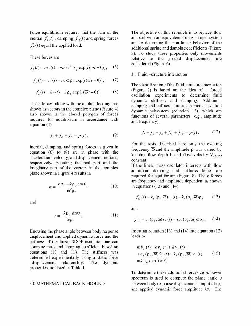
and Yen (2002) use forced oscillation tests to determine fluid and soil coefficients. 2.0 EXPERIMENTAL SET-UP The experimental set-up consists of two major subsystems: a flume to simulate various flow and riverbed conditions and the shaking device to apply different dynamic loadings. 2.1 Flume The flume consists of a 1300 mm long inlet and a 2000 mm straight channel (Figure 1). The upstream flow conditioning is achieved using filter mats, a honeycomb flow straightener, and a carefully designed trumpet-shaped inlet. The flume is designed to have a uniform flow distribution over the width and to have fully developed turbulent flow (following Prandtl’s velocity distribution) at the test section. The recess at the test section is 400 mm x 300 mm (length x width) and 80 mm deep, and can be filled with sand particles of various sizes. The roughness of the fixed bed upstream of the recess can be varied according to the sand particles used in the recess. A 25 l/s pump provides the flume with water, which is stored under the flume in a water tank. A flow meter measures the discharge and an ultra sonic flow depth meter determines the flow depth. A laser distance meter, which is mounted on a portal robot, can scan scour holes during test runs. The flow velocity is measured with an electro magnetic velocity probe. 2.2 Shaking device The shaking device (Figure 2) is mounted above the flume on a rigid frame at the test section. The rigid frame with shaker can be turned 90 degrees and is portable. Two synchronous linear drive motors apply dynamic forces up to 12 Hz. Band limited random noise can be used to simulate earthquake-loading. A ridged model bridge pier is fixed to a platform with linear bearings, which is attached to a linear guide system and mounted elastically to the drive platform. Using different coil springs for the elastical support can vary the natural frequency. The mechanical (structural)
subsystem represents a linear SDOF system, which is lightly damped to study a significant peak resonant response. The damping ratio is determined by the Half-Power (Band-Width) method. The other end of the vertical rigid model pier is mounted in soil to interact with the soil subsystem. The body response displacement is measured with a laser distance meter and the response acceleration with accelerometers. The response velocity is determined by integrating the response acceleration. Two load cells measure the applied dynamic loading. 2.3 Dynamic properties of the linear SDOF
oscillator As shown in Figure 3, the equilibrium of forces can be written
0)()()( =++ tftftf SDI . (1) Substituting for inertial, damping, and elastic forces in equation 1 yields
0 =)(+)(+)( tvktvctvm TT &&& . (2) Before this equation can be solved, all forces must be expressed in terms of a single variable, which can be accomplished by noting the total motion as follows
)(+)(=)( tvtvtv GT . (3) Substituting equation (3) into equation (2) leads to the equation of motion, since the motor displacement represents the specified dynamic input to the structure
)(=)( =)(+)(+)( tptvktvktvctvm GTTT &&& . (4) The dynamic properties can be determined based on the balance of forces acting on the linear mass oscillator under steady state harmonic condition whereby the total response is
)]θ−ω([ρ=)( ttv TT iexp . (5)
Force equilibrium requires that the sum of the inertial , damping and spring forces
equal the applied load. )(tfI )(tfD
)(tfS
These forces are
θ)]−ρω−== tωimtvmtfT
2I ([exp)()( && , (6)
θ)]−ρω== tωicitvctf ΤD ([exp))( (& , (7)
θ)]−ρ== tωiktvktf ΤS ([exp)()( . (8)
These forces, along with the applied loading, are shown as vectors in the complex plane (Figure 4) also shown is the closed polygon of forces required for equilibrium in accordance with equation (4)
)(=++ tpfff SDI . (9) Inertial, damping, and spring forces as given in equation (6) to (8) are in phase with the acceleration, velocity, and displacement motions, respectively. Equating the real part and the imaginary part of the vectors in the complex plane shown in Figure 4 results in
T2
GT kkmρω
θρ−ρ = cos (10)
and
T
Gkcρω
θρ = sin . (11)
Knowing the phase angle between body response displacement and applied dynamic force and the stiffness of the linear SDOF oscillator one can compute mass and damping coefficient based on equations (10 and 11). The stiffness was determined experimentally using a static force –displacement relationship. The dynamic properties are listed in Table 1. 3.0 MATHEMATICAL BACKGROUND
The objective of this research is to replace flow and soil with an equivalent spring damper system and to determine the non-linear behavior of the additional spring and damping coefficients (Figure 5). To study these properties only movements relative to the ground displacements are considered (Figure 6). 3.1 Fluid –structure interaction The identification of the fluid-structure interaction (Figure 7) is based on the idea of a forced oscillation experiments to determine fluid dynamic stiffness and damping. Additional damping and stiffness forces can model the fluid dynamic subsystem (equation 12), which are functions of several parameters (e.g., amplitude and frequency).
)(=++++ tpfffff DFSFSDI . (12) For the tests described here only the exciting frequency ω and the amplitude ρ was varied by keeping flow depth h and flow velocity VFLUID constant. If the linear mass oscillator interacts with flow additional damping and stiffness forces are required for equilibrium (Figure 8). These forces are frequency and amplitude dependent as shown in equations (13) and (14)
TTFTTFSF ,ktv,ktf ρωρ=ωρ= )()()()( (13) and
TTFTTFDF ,citv,cf ρωωρ=ωρ= )()()( & . (14) Inserting equation (13) and (14) into equation (12) leads to
).ω(ρ =)( )ω,ρ(+ )()ω,ρ(+
+)(+)(+ )(
tktvktvc
tvktvctvm
G
TTFTTF
TTT
iexp&
&&&
(15)
To determine these additional forces cross power spectrum is used to compute the phase angle θ between body response displacement amplitude ρT and applied dynamic force amplitude kρG. The
forces can be expressed by equilibrating the dynamic force components
ISGSF ffkf −−θρ= cos (16)
DGDF fkf −θρ= sin . (17) Substituting equations (6) to (8) and equations (13) and (14) into equation (16) and (17), one obtains the fluid coefficient functions
T
T2
TGTF
mkkρ
ρω+ρ−θρ =)ω,ρ( )cos( (18)
T
TGTF
ckcρω
ρω−θρ =)ω,ρ( sin . (19)
3.2 Soil –structure interaction To describe the soil subsystem (Figure 9) again an equivalent damping and stiffness force will be identified. The additional soil forces are plotted in the complex plane as shown in Figure 10. Equilibrating the forces results in
)(=++++ tpfffff DSSSSDI . (20) The soil tests described here only the exciting frequency ω and the amplitude ρ was varied. Non-cohesive soil with D50 = 0.3 mm was used for the soil – structure experiments. The pile depth d (Figure 9) was constant at the beginning of each test. These soil forces are again frequency and amplitude dependent as shown in equations (21) and (22)
TTSTTSSS ,ktv,ktf ρωρ=ωρ= )()()()( (21) and
TTSTTSDS ,citv,cf ρωωρ=ωρ= )()()( & . (22) Inserting equation (21) and (22) into equation (20) leads to
).ω(ρ =)( )ω,ρ(+ )()ω,ρ(+
+)(+)(+ )(
tktvktvc
tvktvctvm
G
TTSTTS
TTT
iexp&
&&&
(23)
Cross power spectrum is used to calculate the phase angle θ between body response displacement amplitude ρT and dynamic force amplitude kρG. Equilibrating the real and imaginary components of the forces results in
ISGSS ffkf −−θρ= cos (24)
DGDS fkf −θρ= sin . (25) Substituting equations (6) to (8) and equations (21) and (22) into equation (24) and (25), to get the soil coefficient functions
T
T2
TGTS
mkkρ
ρω+ρ−θρ =)ω,ρ( )cos( (26)
T
TGTS
ckcρω
ρω−θρ =)ω,ρ( sin . (27)
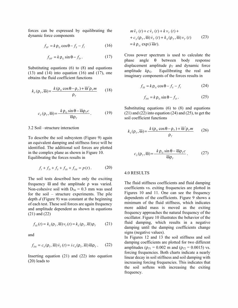
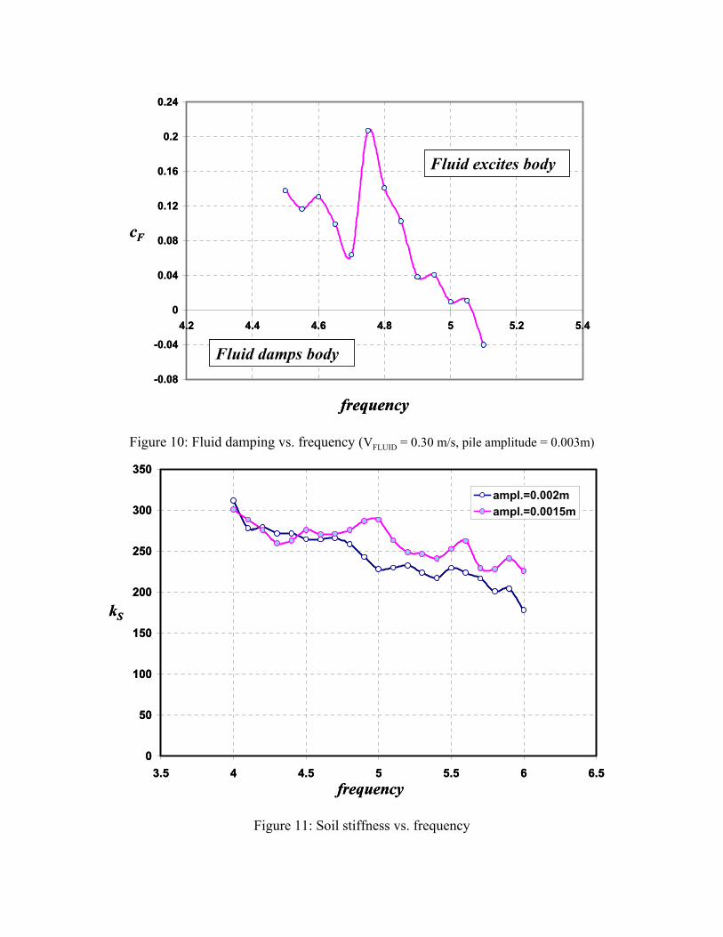
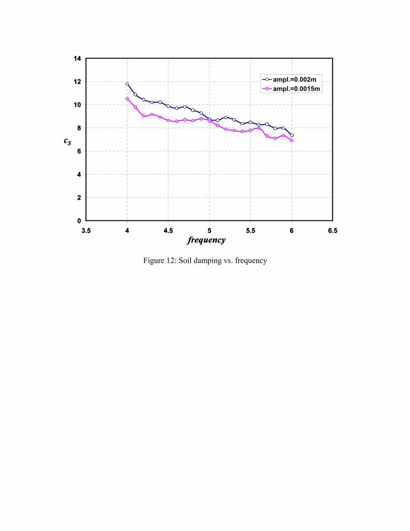
4.0 RESULTS The fluid stiffness coefficients and fluid damping coefficients vs. exiting frequencies are plotted in Figures 10 and 11. One can see the frequency dependents of the coefficients. Figure 9 shows a minimum of the fluid stiffness, which indicates more added mass is moved as the exiting frequency approaches the natural frequency of the oscillator. Figure 10 illustrates the behavior of the fluid damping, which results in a negative damping until the damping coefficients change signs (negative values). In Figures 12 and 13 the soil stiffness and soil damping coefficients are plotted for two different amplitudes (ρT1 = 0.002 m and (ρT2 = 0.0015) vs. forcing frequencies. Both charts indicate a nearly linear decay in soil stiffness and soil damping with increasing forcing frequencies. This indicates that the soil softens with increasing the exiting frequency.
6.0 REFERENCES Deniz S., Staubli T., (1997), Oscillating rectangular and octagonal profiles: Interaction of leading- and trailing-edge vortex formation, Journal of Fluids and Structures, Vol. 11, p. 3-31.
Barowicks, H., (1976), Effects of cross-sectional shape and amplitude on aeroelastic vibrations of sharp-edged prismatic bodies, Doctoral Dissertation, Techn. Universitaet Hannover, Germany.
Kerenyi K., Yen P. W., (2002), Multi Hazard Dynamic Testing for Bridge Piers, Proceedings of the 18th US-Japan Bridge Engineering Workshop, St Luis, Missouri, p. 77-82. Staubli, T., (1983), Investigation of oscillating forces on a vibrating cylinder in cross-flow, Doctoral Dissertation, ETH Zuerich, Switzerland
Scruton, C., (1963),. On the wind-excited oscillations of stacks, towers and masts, 1st Conference wind effects on buildings and structures, Teddington, UK, Paper 16
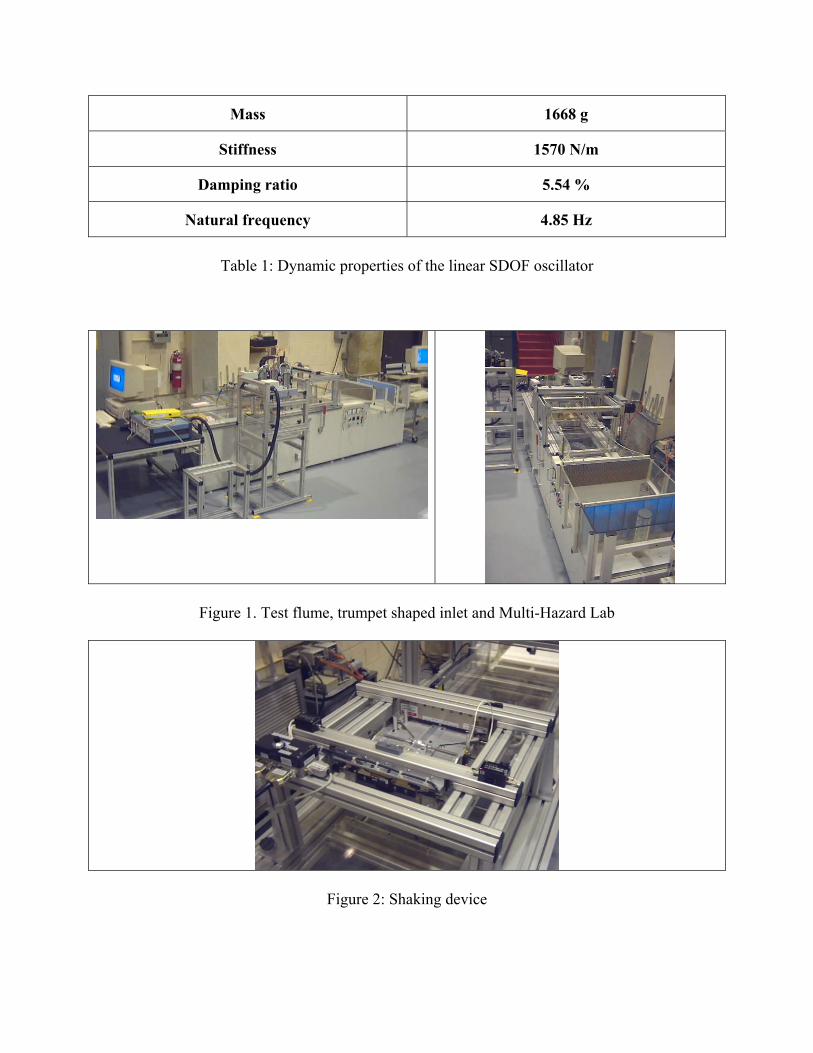
Mass 1668 g
Stiffness 1570 N/m
Damping ratio 5.54 %
Natural frequency 4.85 Hz
Table 1: Dynamic properties of the linear SDOF oscillator
Figure 1. Test flume, trumpet shaped inlet and Multi-Hazard Lab
Figure 2: Shaking device
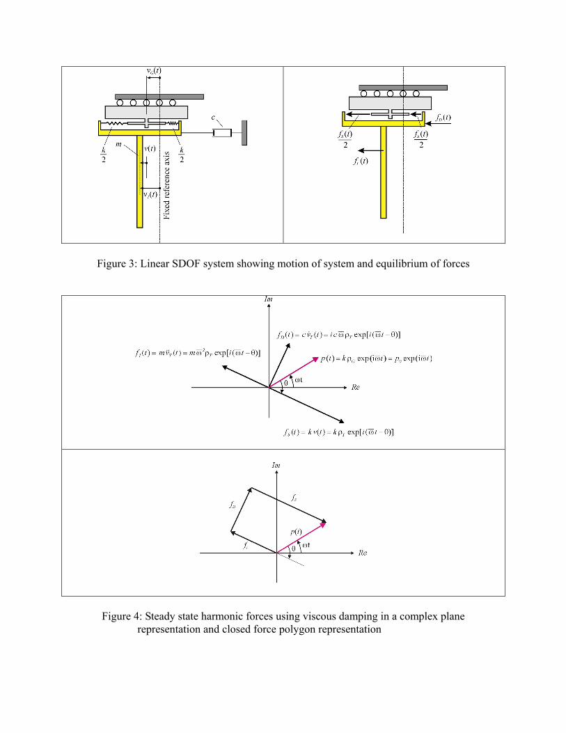
Figure 3: Linear SDOF system showing motion of system and equilibrium of forces
Figure 4: Steady state harmonic forces using viscous damping in a complex plane
representation and closed force polygon representation
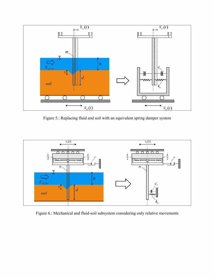
Figure 5.: Replacing fluid and soil with an equivalent spring damper system
Figure 6.: Mechanical and fluid-soil subsystem considering only relative movements
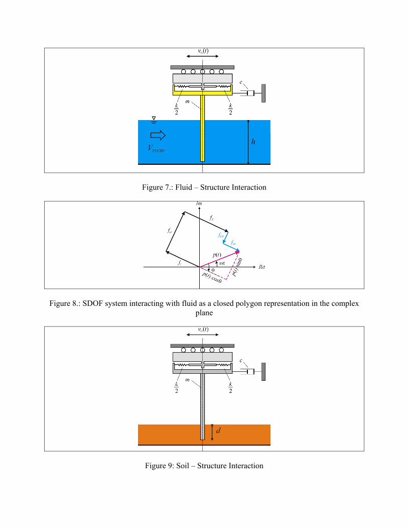
Figure 7.: Fluid – Structure Interaction
Figure 8.: SDOF system interacting with fluid as a closed polygon representation in the complex
plane
Figure 9: Soil – Structure Interaction
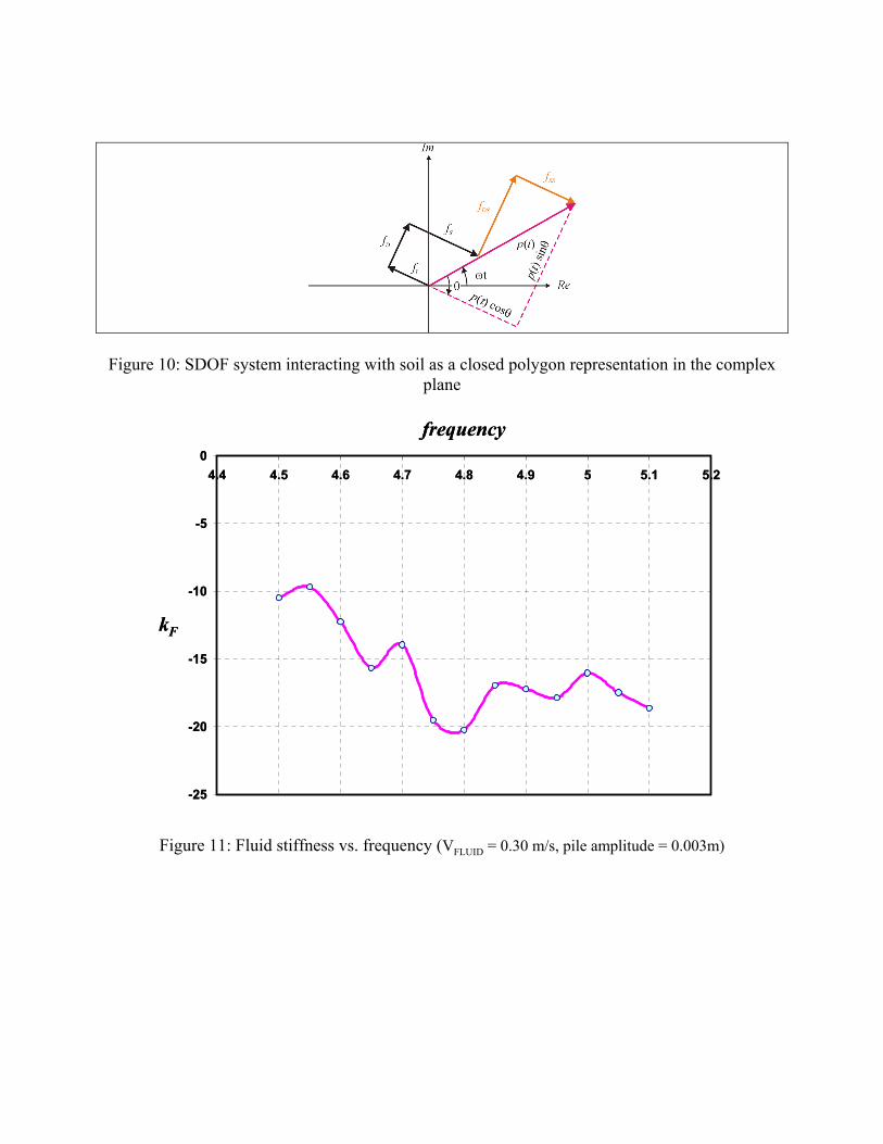
Figure 10: SDOF system interacting with soil as a closed polygon representation in the complex
plane
kF
frequency
-25
-20
-15
-10
-5
04.4 4.5 4.6 4.7 4.8 4.9 5 5.1 5.2
kF
frequency
-25
-20
-15
-10
-5
04.4 4.5 4.6 4.7 4.8 4.9 5 5.1 5.2
Figure 11: Fluid stiffness vs. frequency (VFLUID = 0.30 m/s, pile amplitude = 0.003m)
-0.08
-0.04
0
0.04
0.08
0.12
0.16
0.2
0.24
4.2 4.4 4.6 4.8 5 5.2 5.4
frequency
cF
Fluid excites body
Fluid damps body-0.08
-0.04
0
0.04
0.08
0.12
0.16
0.2
0.24
4.2 4.4 4.6 4.8 5 5.2 5.4
frequency
cF
Fluid excites body
Fluid damps body
Figure 10: Fluid damping vs. frequency (VFLUID = 0.30 m/s, pile amplitude = 0.003m)
kS
frequency
0
50
100
150
200
250
300
350
3.5 4 4.5 5 5.5 6 6.5
ampl.=0.002mampl.=0.0015m
kS
frequency
0
50
100
150
200
250
300
350
3.5 4 4.5 5 5.5 6 6.5
ampl.=0.002mampl.=0.0015m
Figure 11: Soil stiffness vs. frequency
frequency
cS
0
2
4
6
8
10
12
14
3.5 4 4.5 5 5.5 6 6.5
ampl.=0.002mampl.=0.0015m
frequency
cS
0
2
4
6
8
10
12
14
3.5 4 4.5 5 5.5 6 6.5
ampl.=0.002mampl.=0.0015m
Figure 12: Soil damping vs. frequency