FLUX DENSITY MEASUREMENT ON OPEN VOLUMETRIC

RECEIVERS

Felix Göhring1, Olaf Bender

2, Marc Röger

3, Janina Nettlau

4, Peter Schwarzbözl

1

1 German Aerospace Center (DLR), Solar Research, 51147 Cologne, Germany

Phone: +49-2203 601 2994, E-Mail: felix.goehring@dlr.de

2 Technical University of Darmstadt, Reactive Flows and Diagnostics, Germany

3 German Aerospace Center (DLR), Solar Research, Plataforma Solar de Almería, Spain

4 University of Stuttgart, Institute for Thermodynamics and Thermal Engineering, Germany

Abstract

Flux density measurement on external receivers is an important parameter for supervision and control of

commercial and research solar tower power plants. This article presents a flux density measurement system

developed for open volumetric receivers that can be adapted to other receiver systems. Affordable video

camera technique is used and advanced corrections are applied. Main focus is put on the challenge caused by

not perfectly diffuse reflecting receiver surfaces and correction of this effect to achieve reliable measurement

data. For this task the bidirectional reflectance distribution function of the used absorber material has been

determined and employed. The system has been developed and tested by the German Aerospace Center

(DLR) at the Plataforma Solar de Almería and the Solar Tower Jülich.

Keywords: flux density, flux distribution, bidirectional reflectance distribution function, gonioreflectometer

1. Introduction

Flux density measurement on external receivers is an important parameter for supervision and control of

commercial and research solar tower power plants. It is a valuable input for control systems, operators,

complex simulation models and is necessary for performance assessment of receiver and heliostat field. As

indirect flux measurement with moving bars needs additional hardware and gets more difficult with larger

receiver apertures, flux could be measured directly on the receiver surface at external receivers. Tests on the

Plataforma Solar de Almería (PSA) demonstrated the feasibility of this task on small-scale receivers [1]. The

technology has been applied to the Solar Power Tower Jülich (STJ), a demonstration power plant with an

open volumetric receiver and nominal electric output of 1.5 MW [2], and the correction methodology has

been elaborated in detail.

2. Indirect flux density measurement

In laboratory and test scale receivers flux measurement is often done by moving a reflecting target with

Lambertian characteristics through the focus while a CCD-camera detects the reflected brightness which is

proportional to the intensity of the reflected irradiation [3]. As this method needed installation of a large

moving bar at the 22 m² receiver at STJ, another system was developed that basically detects the reflected

radiation from the absorber surface and applies corrections and calibrations to account for the non-

Lambertian characteristics and inhomogeneous reflectivities of the absorber cups.

The heliostat field of STJ consists of 2153 heliostats with almost flat mirrors and a total area of around

18 000 sqm. The control system allows free choice of aimpoints. Aiming point optimization for achieving

best flux distribution during operation of the receiver at different loads is of great interest for ongoing work.

2.1 General setup and measurement system

The CCD-camera that captures the raw images is located between heliostat field and tower (Fig. 1) to avoid

effects of retroreflection that cause difficulties to exactly quantify reflections to the camera. The receiver at

STJ that is monitored by the camera consists of 1080 SiC absorber cups arranged in 36 rows and 30 columns

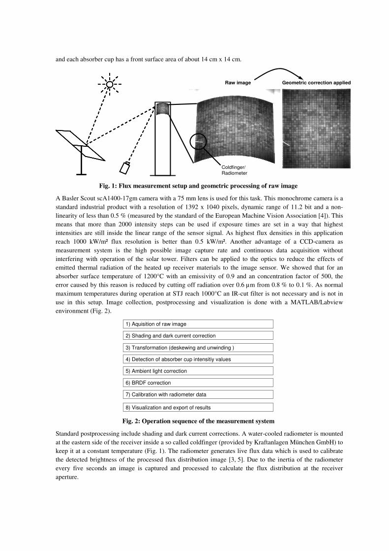
and each absorber cup has a front surface area of about 14 cm x 14 cm.

Coldfinger/

Radiometer

Raw image Geometric correction applied

Fig. 1: Flux measurement setup and geometric processing of raw image

A Basler Scout scA1400-17gm camera with a 75 mm lens is used for this task. This monochrome camera is a

standard industrial product with a resolution of 1392 x 1040 pixels, dynamic range of 11.2 bit and a non-

linearity of less than 0.5 % (measured by the standard of the European Machine Vision Association [4]). This

means that more than 2000 intensity steps can be used if exposure times are set in a way that highest

intensities are still inside the linear range of the sensor signal. As highest flux densities in this application

reach 1000 kW/m² flux resolution is better than 0.5 kW/m². Another advantage of a CCD-camera as

measurement system is the high possible image capture rate and continuous data acquisition without

interfering with operation of the solar tower. Filters can be applied to the optics to reduce the effects of

emitted thermal radiation of the heated up receiver materials to the image sensor. We showed that for an

absorber surface temperature of 1200°C with an emissivity of 0.9 and an concentration factor of 500, the

error caused by this reason is reduced by cutting off radiation over 0.6 µm from 0.8 % to 0.1 %. As normal

maximum temperatures during operation at STJ reach 1000°C an IR-cut filter is not necessary and is not in

use in this setup. Image collection, postprocessing and visualization is done with a MATLAB/Labview

environment (Fig. 2).

1) Aquisition of raw image

2) Shading and dark current correction

3) Transformation (deskewing and unwinding )

5) Ambient light correction

4) Detection of absorber cup intensitiy values

6) BRDF correction

7) Calibration with radiometer data

8) Visualization and export of results

Fig. 2: Operation sequence of the measurement system

Standard postprocessing include shading and dark current corrections. A water-cooled radiometer is mounted

at the eastern side of the receiver inside a so called coldfinger (provided by Kraftanlagen München GmbH) to

keep it at a constant temperature (Fig. 1). The radiometer generates live flux data which is used to calibrate

the detected brightness of the processed flux distribution image [3, 5]. Due to the inertia of the radiometer

every five seconds an image is captured and processed to calculate the flux distribution at the receiver

aperture.

2.2 Postprocessing and visualization

After data collection, shading and dark current corrections are applied to the raw image [3, 5]. A transformed

flat image of the receiver surface is beneficial for effective image processing. Therefore, the image is

deskewed and unwinded. As the camera position and orientation is not totally stable (e.g. influence

temperature and wind), the receiver corners are detected automatically for the processing of each single

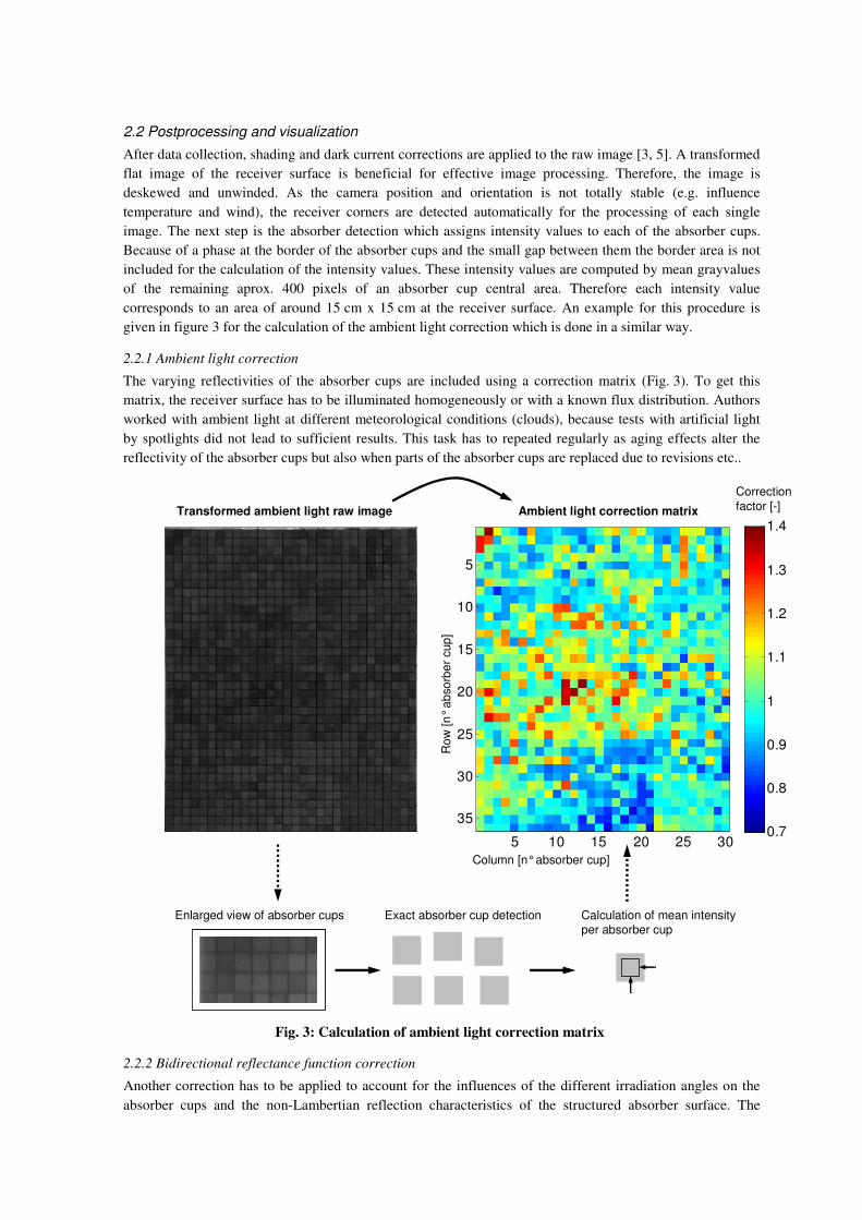
image. The next step is the absorber detection which assigns intensity values to each of the absorber cups.

Because of a phase at the border of the absorber cups and the small gap between them the border area is not

included for the calculation of the intensity values. These intensity values are computed by mean grayvalues

of the remaining aprox. 400 pixels of an absorber cup central area. Therefore each intensity value

corresponds to an area of around 15 cm x 15 cm at the receiver surface. An example for this procedure is

given in figure 3 for the calculation of the ambient light correction which is done in a similar way.

2.2.1 Ambient light correction

The varying reflectivities of the absorber cups are included using a correction matrix (Fig. 3). To get this

matrix, the receiver surface has to be illuminated homogeneously or with a known flux distribution. Authors

worked with ambient light at different meteorological conditions (clouds), because tests with artificial light

by spotlights did not lead to sufficient results. This task has to repeated regularly as aging effects alter the

reflectivity of the absorber cups but also when parts of the absorber cups are replaced due to revisions etc..

200 400 600 800 1000

200

400

600

800

1000

1200

5 10 15 20 25 30

5

10

15

20

25

30

350.7

0.8

0.9

1

1.1

1.2

1.3

1.4

Ro

w[n

°a

bso

rbe

rcup

]

Column [n°absorber cup]

Correction

factor [-]Transformed ambient light raw image Ambient light correction matrix

Enlarged view of absorber cups Exact absorber cup detection Calculation of mean intensityper absorber cup

Fig. 3: Calculation of ambient light correction matrix

2.2.2 Bidirectional reflectance function correction

Another correction has to be applied to account for the influences of the different irradiation angles on the

absorber cups and the non-Lambertian reflection characteristics of the structured absorber surface. The

bidirectional reflectance distribution function (BRDF) is constant for perfect diffuse reflecting materials but

for real surfaces it depends on ray incidence angles and observation angles. The BRDF is a four dimensional

function that is defined as the ratio between incidence and reflected radiance [6, 7]:

( , , , )( , , , )

( , ) cos d

r r r

r r

L θ φ θ φρ θ φ θ φ

L θ φ θ Ω=

The unit of BRDF is [sr-1

]. As in this work the BRDF values are only compared to those determined with the

same device the raw sensor signals are used for calculations and presentations and the sensor unit [mV] is

omitted.

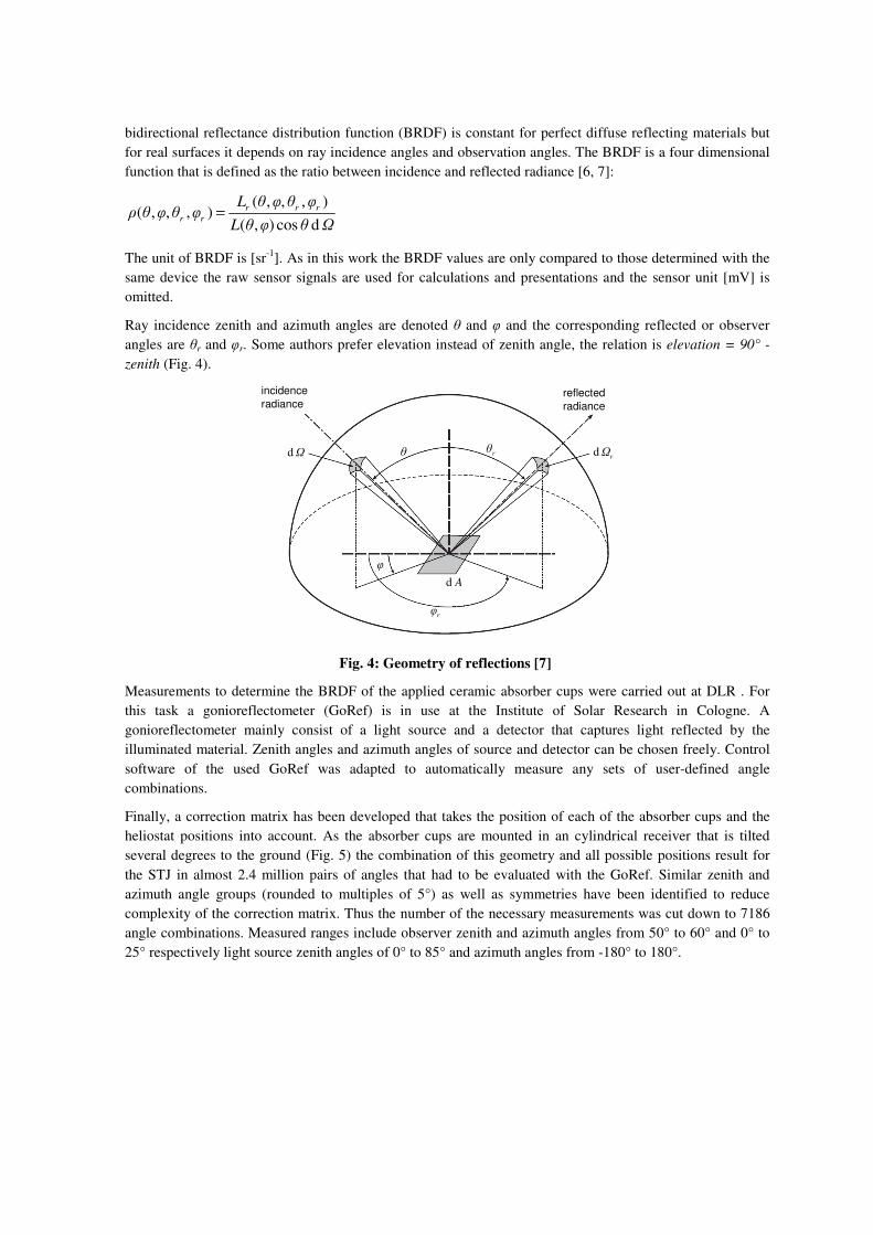
Ray incidence zenith and azimuth angles are denoted θ and φ and the corresponding reflected or observer

angles are θr and φr. Some authors prefer elevation instead of zenith angle, the relation is elevation = 90° -

zenith (Fig. 4).

θ rθ

rφ

φ

d A

d rΩdΩ

incidence

radiancereflected

radiance

θ rθ

rφ

φ

d A

d rΩdΩ

incidence

radiancereflected

radiance

Fig. 4: Geometry of reflections [7]

Measurements to determine the BRDF of the applied ceramic absorber cups were carried out at DLR . For

this task a gonioreflectometer (GoRef) is in use at the Institute of Solar Research in Cologne. A

gonioreflectometer mainly consist of a light source and a detector that captures light reflected by the

illuminated material. Zenith angles and azimuth angles of source and detector can be chosen freely. Control

software of the used GoRef was adapted to automatically measure any sets of user-defined angle

combinations.

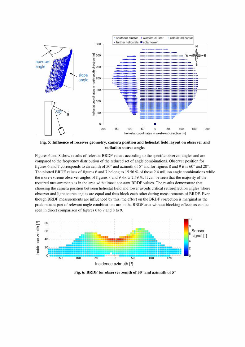
Finally, a correction matrix has been developed that takes the position of each of the absorber cups and the

heliostat positions into account. As the absorber cups are mounted in an cylindrical receiver that is tilted

several degrees to the ground (Fig. 5) the combination of this geometry and all possible positions result for

the STJ in almost 2.4 million pairs of angles that had to be evaluated with the GoRef. Similar zenith and

azimuth angle groups (rounded to multiples of 5°) as well as symmetries have been identified to reduce

complexity of the correction matrix. Thus the number of the necessary measurements was cut down to 7186

angle combinations. Measured ranges include observer zenith and azimuth angles from 50° to 60° and 0° to

25° respectively light source zenith angles of 0° to 85° and azimuth angles from -180° to 180°.

apertureangle

slopeangle

nr

50°

0

50

100

150

200

250

300

350

-200 -150 -100 -50 0 50 100 150 200

heliostat coordinates in west-east direction [m]

helio

sta

t coord

inate

s in n

ort

h-s

outh

direction [

m]

southern cluster western cluster calculated center

further heliostats solar tower

N

EW

S

Fig. 5: Influence of receiver geometry, camera position and heliostat field layout on observer and

radiation source angles

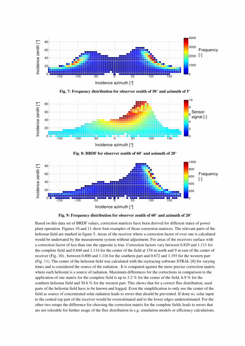
Figures 6 and 8 show results of relevant BRDF values according to the specific observer angles and are

compared to the frequency distribution of the reduced set of angle combinations. Observer position for

figures 6 and 7 corresponds to an zenith of 50° and azimuth of 5° and for figures 8 and 9 it is 60° and 20°.

The plotted BRDF values of figures 6 and 7 belong to 15.56 % of those 2.4 million angle combinations while

the more extreme observer angles of figures 8 and 9 show 2.59 %. It can be seen that the majority of the

required measurements is in the area with almost constant BRDF values. The results demonstrate that

choosing the camera position between heliostat field and tower avoids critical retroreflection angles where

observer and light source angles are equal and thus block each other during measurements of BRDF. Even

though BRDF measurements are influenced by this, the effect on the BRDF correction is marginal as the

predominant part of relevant angle combinations are in the BRDF area without blocking effects as can be

seen in direct comparison of figures 6 to 7 and 8 to 9.

-150 -100 -50 0 50 100 1500

20

40

60

80

0

2

4

6

8

10

Incidence azimuth [°]

Incid

ence

zenith

[°]

Sensor

signal [-]

Fig. 6: BRDF for observer zenith of 50° and azimuth of 5°

-150 -100 -50 0 50 100 1500

20

40

60

80

0

1000

2000

3000

4000

Incidence azimuth [°]

Incid

ence

zenith

[°]

Frequency

[-]

Fig. 7: Frequency distribution for observer zenith of 50° and azimuth of 5°

-150 -100 -50 0 50 100 1500

20

40

60

80

0

2

4

6

8

10

Incidence azimuth [°]

Incid

ence

zenith

[°]

Sensor

signal [-]

Fig. 8: BRDF for observer zenith of 60° and azimuth of 20°

-150 -100 -50 0 50 100 1500

20

40

60

80

0

200

400

600

800

1000

Frequency

[-]

Incidence azimuth [°]

Incid

ence

zenith

[°]

Fig. 9: Frequency distribution for observer zenith of 60° and azimuth of 20°

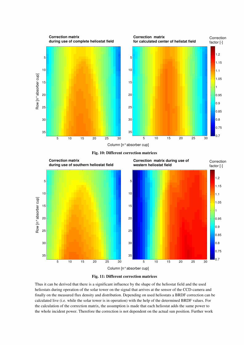
Based on this data set of BRDF values, correction matrices have been derived for different states of power

plant operation. Figures 10 and 11 show four examples of those correction matrices. The relevant parts of the

heliostat field are marked in figure 5. Areas of the receiver where a correction factor of over one is calculated

would be underrated by the measurement system without adjustment. For areas of the receivers surface with

a correction factor of less than one the opposite is true. Correction factors vary between 0.829 and 1.111 for

the complete field and 0.840 and 1.114 for the center of the field at 154 m north and 9 m east of the center of

receiver (Fig. 10) , between 0.800 and 1.116 for the southern part and 0.672 and 1.193 for the western part

(Fig. 11). The center of the heliostat field was calculated with the raytracing software STRAL [8] for varying

times and is considered the source of the radiation . It is compared against the more precise correction matrix

where each heliostat is a source of radiation. Maximum differences for the corrections in comparison to the

application of one matrix for the complete field is up to 3.2 % for the center of the field, 6.9 % for the

southern heliostat field and 30.6 % for the western part. This shows that for a correct flux distribution, used

parts of the heliostat field have to be known and logged. Even the simplification to only use the center of the

field as source of concentrated solar radiation leads to errors that should be prevented. If done so, solar input

to the central top part of the receiver would be overestimated and to the lower edges underestimated. For the

other two setups the difference for choosing the correction matrix for the complete fields leads to errors that

are not tolerable for further usage of the flux distribution in e.g. simulation models or efficiency calculations.

5 10 15 20 25 30

5

10

15

20

25

30

35

5 10 15 20 25 30

5

10

15

20

25

30

35

0.7

0.75

0.8

0.85

0.9

0.95

1

1.05

1.1

1.15

1.2

Column [n°absorber cup]

Row

[n°

absorb

er

cup

]Correction

factor [-]

Correction matrixduring use of complete heliostat field

Correction matrixfor calculated center of helistat field

Fig. 10: Different correction matrices

5 10 15 20 25 30

5

10

15

20

25

30

35

5 10 15 20 25 30

5

10

15

20

25

30

35

0.7

0.75

0.8

0.85

0.9

0.95

1

1.05

1.1

1.15

1.2

Column [n°absorber cup]

Row

[n°

absorb

er

cup

]

Correction

factor [-]

Correction matrixduring use of southern heliostat field

Correction matrix during use ofwestern heliostat field

Fig. 11: Different correction matrices

Thus it can be derived that there is a significant influence by the shape of the heliostat field and the used

heliostats during operation of the solar tower on the signal that arrives at the sensor of the CCD-camera and

finally on the measured flux density and distribution. Depending on used heliostats a BRDF correction can be

calculated live (i.e. while the solar tower is in operation) with the help of the determined BRDF values. For

the calculation of the correction matrix, the assumption is made that each heliostat adds the same power to

the whole incident power. Therefore the correction is not dependent on the actual sun position. Further work

will compare this against correction matrices that include cosine and atmospheric losses and uncertainties in

heliostat tracking and aimpoint control and therefore have to be calculated for the exact time of the

acquisition of the flux distribution.

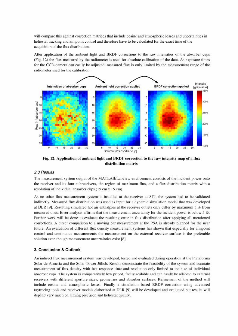
After application of the ambient light and BRDF corrections to the raw intensities of the absorber cups

(Fig. 12) the flux measured by the radiometer is used for absolute calibration of the data. As exposure times

for the CCD-camera can easily be adjusted, measured flux is only limited by the measurement range of the

radiometer used for the calibration.

Row

[n°

abso

rber

cup]

5 10 15 20 25 30

5

10

15

20

25

30

35

5 10 15 20 25 30

5

10

15

20

25

30

35

5 10 15 20 25 30

5

10

15

20

25

30

351000

1500

2000

2500

3000

3500

Intensity[grayvalue]

Column [n°absorber cup]

Intensities of absorber cups Ambient light correction applied BRDF correction applied

Fig. 12: Application of ambient light and BRDF correction to the raw intensity map of a flux

distribution matrix

2.3 Results

The measurement system output of the MATLAB/Labview environment consists of the incident power onto

the receiver and its four subreceivers, the region of maximum flux, and a flux distribution matrix with a

resolution of individual absorber cups (15 cm x 15 cm).

As no other flux measurement system is installed at the receiver at STJ, the system had to be validated

indirectly. Measured flux distribution was used as input for a dynamic simulation model that was developed

at DLR [9]. Resulting simulated hot air enthalpies at the receiver outlets only differ by maximum 5 % from

measured ones. Error analysis affirms that the measurement uncertainty for the incident power is below 5 %.

Further work will be done to evaluate the resulting error in flux distribution after applying all mentioned

corrections. A direct comparison to a moving bar measurement at the PSA is already planned for the near

future. An evaluation of different flux density measurement systems has shown that especially for aimpoint

control and continuous measurements the measurement on the external receiver surface is the preferable

solution even though measurement uncertainties exist [8].

3. Conclusion & Outlook

An indirect flux measurement system was developed, tested and evaluated during operation at the Plataforma

Solar de Almería and the Solar Tower Jülich. Results demonstrate the feasibility of the system and accurate

measurement of flux density with fast response time and resolution only limited to the size of individual

absorber cups. The system is comparatively low priced, freely scalable and can easily be adapted to external

receivers with different aperture sizes, geometries and absorber surfaces. Refinement of the method will

include cosine and atmospheric losses. Finally a simulation based BRDF correction using advanced

raytracing tools and receiver models elaborated at DLR [9] will be developed and evaluated but results will

depend very much on aiming precision and heliostat quality.

Acknowledgments

Financial support from the German Federal Ministry for the Environment, Nature Conservation and Nuclear

Safety, the Ministries of Economic Affairs of the States of North Rhine-Westphalia and Bavaria are

gratefully acknowledged. We also thank Stadtwerke Jülich GmbH for operating the power plant and their

support, Kraftanlagen München GmbH for supplying the STJ with coldfingers and radiometers and

integrating them into the process control system and Markus Pfänder for his valuable contributions during the

early development phase of this work.

References

[1] M. Röger, P. Herrmann, M. Ebert, C. Prahl, S. Ulmer, F. Göhring, Flux density measurement on large-

scale receivers, Proceedings of SolarPACES 2011, Granada, Spain, Sept. 20-23 (2011)

[2] S. Pomp, P. Schwarzbözl, G. Koll, F. Göhring, T. Hartz, M. Schmitz, B. Hoffschmidt, The Solar Tower

Jülich – First Operational Experiences and Test Results, Proceedings of 16th

SolarPACES, Perpignan,

France, Sep. 21-24, 2010

[3] S. Ulmer, Messung der Strahlungsflussdichteverteilung von punktkonzentrierenden solarthermischen

Kraftwerken, VDI-Verlag GmbH, Düsseldorf, 2004

[4] European Machine Vision Association: EMVA Standard 1288 – Standard for Characterization and

Presentation of Specification Data for Image Sensors and Cameras (Release A1.03), 2006

[5] E. Lüpfert, P. Heller, Steffen Ulmer, R. Monterreal, J. Fernández, Concentrated solar radiation

measurement with video image processing and online fluxgage calibration. Solar Thermal 2000

International Conference Sydney, Australia, March 8-10 (2000)

[6] R. Siegel, J. R. Howell, Wärmeübertragung durch Strahlung, Springer-Verlag, Berlin, 1988

[7] J. Gengenbach, REM-Berechnung und Messung des Emissionsgrades mikrostrukturierter Oberflächen,

Helmut-Schmidt-Universität, Universität der Bundeswehr Hamburg, 2007

[8] Belhomme, B., Pitz-Paal, R., Schwarzbözl, P., Ulmer, S., New Fast Ray Tracing Tool for High-Precision

Simulation of Heliostat Fields, Journal of Solar Energy Engineering, 131, 3 (2009), 031002-031008.

[9] N. Ahlbrink, J. Anderson, M. Diehl, D. Maldonado Quinto, R. Pitz-Paal, Optimized Operation of an Open

Volumetric Air Receiver, Proceedings of 16th

SolarPACES, Perpignan, France, Sep. 21-24, 2010