FluxLetter Vol.5 No. 2 March 2013

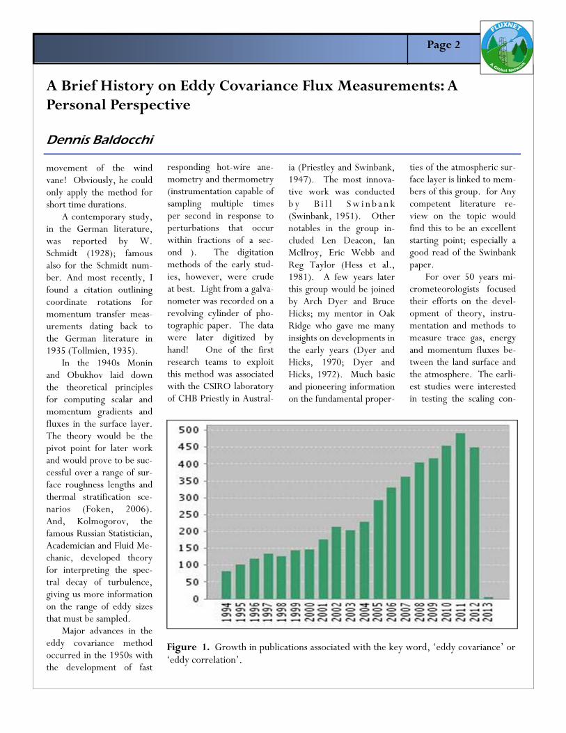
Because so many prac-titioners are new to the field of eddy covariance flux measurements, we felt it would be a good time to provide a short and broad history on the topic of flux-es in general and focusing on eddy covariance. The field of eddy co-variance has experienced rapid, exponential growth since the 1990s due to a convergence of develop-ments in instrumentation, personal computers, data storage devices and advanc-es in micrometeorological theory; Figure 1 shows the growth in publications asso-ciated with the key word, eddy covariance. As I write this history, the web of science informs me that nearly 5000 papers

FluxLetter The Newsletter of FLUXNET

Vol.5 No. 2 March 2013

In This Issue:

A brief hstory on eddy covar-iance flux measurements: A personal perspective Dennis Baldocchi….....Pages 1-8

The Yatir Forest: Post-cards from the edge Dan Yakir……..….Pages 9-11

Solving the energy dissi-pation riddle in Yatir Eyal Rotenberg….....Pages 12-14

The Yatir Forest Site: Decoup-ling phenology to maximize carbon uptake Kadmiel Maseyk..….Pages 15-17

Decoupling of the tree hydraulic components in Yatir Forest Tamir Klein..….…Pages 18-19

Ecohydrology of Yatir – a forest growing in the desert Naama Raz-Yaseef..Pages 20-22

Backing up the flux meaure-ments in the Yatir Forest José M. Grünzweig ..Pages 23-24

The Yatir Forest Site: The nitrogen perspective Ilya Gelfand……...Pages 25-26

A Tribute to Shashi Verma Dennis Baldocchi....Pages 27-28

35 years of urban climate research at the ‘Vancouver-Sunset’ flux tower Andreas Christen, Tim Oke , Sue Grimmond, Douw Steyn and Matthias Roth…....Pages 29-37

have been published that are linked to the key words ‘eddy covariance’ or ‘eddy correlation’. Micrometeorology The idea of using mi-crometeorological methods to assess mass and energy exchange can be traced back to before and around the turn of the 20th Centu-ry. The concept of Fickian diffusion led early fluid me-chanics, such as Ludwig Prandtl, G.I. Taylor and Bowen (1920s), to propose the flux-gradient approach, as a concept for evaluating fluxes of momentum, water and heat. Sir Osborne Reynolds (Reynolds, 1895) is credit-ed with devising the theo-

retical idea of the eddy co-variance method after he laid down his famous con-cept of Reynolds averaging. Application of this method was delayed many years due to technical reasons as it relies on fast anemometry and meteorology. One of the first applications of this method was applied in 1926 and was reported by F.J. Scrase (1930, Some charac-teristics of eddy motion in the atmosphere, Geophysi-cal Memoirs, #52, Meteor-ological Office. London, 56 pp). His instrumentation and digitization methods, however, were quite primi-tive. He evaluated the three wind vectors using rapid measurements of wind speed and wind direc-tion. He digitized the data by photographing the wind meter dial and using a kine-matograph to record the

A Brief History on Eddy Covariance Flux Measurements: A Personal Perspective Dennis Baldocchi

In this issue of the FLUXLETTER, we present two historical accounts; one is a history of flux measurements using the eddy covariance method. The sec-ond is a history of the development of flux measurements specific to urban ecosystems. We also profile the Yatir Forest in Israel; a pine forest established at the semi-arid dry timberline. Lastly, Dennis Baldocchi offers a tribute to Shashi Verma; a pioneer in the flux community who has recently retired.

Editors: Laurie Koteen and Dennis Baldocchi, The FLUXNET Office at the University of California, Berkeley

Page 2


responding hot-wire ane-mometry and thermometry (instrumentation capable of sampling multiple times per second in response to perturbations that occur within fractions of a sec-ond ). The digitation methods of the early stud-ies, however, were crude at best. Light from a galva-nometer was recorded on a revolving cylinder of pho-tographic paper. The data were later digitized by hand! One of the first research teams to exploit this method was associated with the CSIRO laboratory of CHB Priestly in Austral-

ia (Priestley and Swinbank, 1947). The most innova-tive work was conducted b y B i l l S w i n b a n k (Swinbank, 1951). Other notables in the group in-cluded Len Deacon, Ian McIlroy, Eric Webb and Reg Taylor (Hess et al., 1981). A few years later this group would be joined by Arch Dyer and Bruce Hicks; my mentor in Oak Ridge who gave me many insights on developments in the early years (Dyer and Hicks, 1970; Dyer and Hicks, 1972). Much basic and pioneering information on the fundamental proper-

ties of the atmospheric sur-face layer is linked to mem-bers of this group. for Any competent literature re-view on the topic would find this to be an excellent starting point; especially a good read of the Swinbank paper. For over 50 years mi-crometeorologists focused their efforts on the devel-opment of theory, instru-mentation and methods to measure trace gas, energy and momentum fluxes be-tween the land surface and the atmosphere. The earli-est studies were interested in testing the scaling con-

movement of the wind vane! Obviously, he could only apply the method for short time durations. A contemporary study, in the German literature, was reported by W. Schmidt (1928); famous also for the Schmidt num-ber. And most recently, I found a citation outlining coordinate rotations for momentum transfer meas-urements dating back to the German literature in 1935 (Tollmien, 1935). In the 1940s Monin and Obukhov laid down the theoretical principles for computing scalar and momentum gradients and fluxes in the surface layer. The theory would be the pivot point for later work and would prove to be suc-cessful over a range of sur-face roughness lengths and thermal stratification sce-narios (Foken, 2006). And, Kolmogorov, the famous Russian Statistician, Academician and Fluid Me-chanic, developed theory for interpreting the spec-tral decay of turbulence, giving us more information on the range of eddy sizes that must be sampled. Major advances in the eddy covariance method occurred in the 1950s with the development of fast

Figure 1. Growth in publications associated with the key word, ‘eddy covariance’ or ‘eddy correlation’.

Page 3


rized in Foken (Foken, 2006). The publication of Workshop on Micromete-orology in 1973 summa-rized the many field exper-iments and codified many of the theories that are used to this day. In the 1970s, theoretical advances in boundary layer meteor-ology were led by J. Deardorff. He developed early models on surface boundary layer fluxes, large eddy simulation and mixing layer theory ( D e a r d o r f f , 1 9 7 2 ; Deardorff, 1978). du Pont Donaldson is credited with introducing higher order closure theory to microme-teorology and K. Shankar Rao and John Wyngaard are among the first who applied higher order clo-sure theory to describe advection (Rao et al., 1974).

Ag/Forest Meteorology By the early 1960s, many concepts pioneered by micrometeorologists, such as Swinbank and co-workers, were ready for practical application to agricultural and ecological problems. Among the first experimentalists to apply flux-gradient theory to

assess CO2 and water vapor exchange over crops in-cluded E. Inoue (1957, Japan), John Monteith ((Monteith and Szeicz, 1960), Sutton Bonnington and Nottingham), Champ Tanner (1960, Univ Wis-consin), Ed Lemon (1962, Cornell), Tom Denmead (1966, CSIRO, Australia), and Norm Rosenberg (1966, Univ. Nebraska). It is my understanding that Dr. Inoue was a developer of the Zero airplane that was used by kamikaze pi-lots during World War 2 by the Japanese. The de-militarization of Japan fol-lowing the War enabled Inoue to apply his skills towards peaceful activities like agriculture and crop production. Among the other important technical advances were the develop-ment of the net radiometer by Verner Suomi, as well as his contributions to the development of the sonic anemometer, with Joost Businger and J.C. Kaimal. Tanner made many advanc-es in wet bulb psychrome-try, which lended itself towards measuring water vapor fluxes with gradient methods. With the success of micrometeorological meas-urements over short vege-

tation came a desire to ap-ply them over tall vegeta-tion. A number of pio-neering flux studies were conducted between the late 1960s and early 1970s. Tom Denmead (Denmead, 1969) , Baumgar tner (Baumgartner A, 1969), Jarvis et al.(Jarvis et al., 2007) and Lemon et al (Lemon et al., 1970) were among the first investiga-tors to apply flux-gradient methods over forests. Coyne and Kelley (Coyne and Kelley, 1975), Saugier and Ripley (Saugier and Ripley, 1978) were among the earliest ecologist to make CO2 measurements over native ecosystems, such as tundra and grass-lands, respectively. Researchers soon found that forests did not operate like tall crops. A series of measurements at Thetford forest in England by Raupach (Raupach, 1979; Raupach and Legg, 1984), Stewart, Gash, Thom and colleagues (Stewart and Thom, 1973) drew atten-tion to the fact that the application of flux gradient theory would prove to be troublesome over tall for-ests. Evidence was grow-ing showing that Monin-Obukhov scale theory—a theory that was successfully

cepts of Monin and Obu-khov, understanding the spectral properties of tur-bulence and the statistical properties of turbulence in the surface boundary layer during stable, neutral and unstable thermal stratifica-tion. Many of the earliest micrometeorological stud-ies were conducted over very ideal landscapes. These locales consisted of extremely level terrain with negligible or short vegetation and were in windy and sunny climes where atmospheric condi-tions could be expected to be steady. Examples in-clude the O’Neill, Nebras-ka (Project Prairie Grass, Lettau and Davidson, 1 9 5 7) , t he K a ns a s (Businger, 1971; Kaimal and Wyngaard, 1990) and Davis (Pruitt et al., 1973) experiments in North America, the Aus-tralian Wangara experi-ment (Hess et al., 1981) and its predecessors near Hay and Kerang (Swinbank and Dyer, 1967) and stud-ies near Tsimlyanskoye in Russia (Zilitinkevich and Chalikov, 1968). These are powerful datasets still being used to parameterize and model surface layer turbulence and are summa-

Page 4

method on aircraft to measure eddy fluxes across landscapes (Desjardins et al., 1982). In the late 1970s, the US Department of Energy funded Lawrence Livermore Laboratory to develop and build open path CO2 sensors. Three sensors were built and were used in a series of pioneering flux measure-ments over crops by Shashi Verma and students in Ne-braska (Anderson and Ver-ma, 1985; Anderson et al., 1984) and by Marv Wesely and colleagues at Argonne (Wesely et al., 1983). And in Japan, E. Ohtaki suc-cessfully developed an in-strument that was applied over rice (Ohtaki, 1984). The logistical difficul-ties associated with making micrometeorological flux-gradient measurements over forests lead to a rela-tive hiatus on mass and energy studies over forests between the mid 70’s and mid 80’s (Paul Jarvis, per-sonal communication). Exceptions included forest meteorology studies in Germany and Sweden using the Flux-Gradient method. The development and commercial availability of sonic anemometers (Kaimal and Businger, 1963), fast response hy-

grometry, and infrared spectrometry (Auble and Meyers 1992; Hyson and Hicks, 1975; Ohtaki and Matsui, 1982) in the 1980/90s lead to a renais-sance of work in the eddy covariance field. It is im-portant to note that studies in this era were based on datasets that consisted of tens of hours of data. The sensors drifted and had to be calibrated frequently. Computer data storage media were small, and in-vestigators tended to baby sit their instruments for each moment of data col-lection. Among the first mod-ern eddy covariance studies over forests were sets of measurements conducted in the early 1980s by the ATDD/NOAA lab in Oak Ridge, TN (McMillen, 1988; Verma et al., 1986), the Institute of Hydrology i n t h e A m a z o n (Shuttleworth, 2007; Shut-tleworth et al., 1984), Ar-gonne National Lab (Wesely et al., 1983) and the CSIRO Centre for En-vironmental Mechanics (Denmead, 1984; Den-mead and Bradley, 1987). The studies of Denmead and colleagues were partic-ularly revolutionary, as they were among the first

to directly measure counter-gradient transfer inside forest canopies. Until the 1990s, open and closed path CO2 sen-sors remained a rare quan-tity. The development of a home-made open path CO2 sensor by Auble and Meyers at the NOAA At-mospheric Turbulence and Diffusion Laboratory in Oak Ridge, TN,(Auble and Meyers 1992) changed this course. They were able to produce tens of sensors that were soon purchased and implemented by col-leagues in Oregon and San Diego. Simultaneously, LICOR was making ad-vances in producing a closed path sensor that used a solid state detector, that enabled one to con-duct eddy covariance meas-urements. These advances, and further developments in computers and data stor-age, lead to a new genera-tion of studies that started collecting data for hun-dreds of hours and tens of days at a time. The cited technical advancements correspond-ed with the political and scientific decision to con-duct large-scale multi-investigator experiments (Shuttleworth, 2007).

predicting gradient behav-ior over short vegetation--breaks down within the roughness layer over tall forests. Direct measure-ments were showing that eddy exchange coefficients were enhanced by turbu-lent transport because the turbulence length scales are long compared to the length scale of scalar gradi-ents (Garratt, 1978; Raupach, 1979). Meas-urements over forests also have logistical difficulties, which arise from the need to suspend delicate instru-mentation tens of meters above the ground. The efficient turbulent mixing afforded by tall forests also caused vertical gradients of scalar properties to be small and difficult to re-solve. One of the first appli-cations of the eddy covari-ance method to agricultural meteorology and on the subject of carbon dioxide exchange occurred in the late 1960s. This work is a t t r i b u t e d t o R a y Desjardins; a graduate stu-dent of Ed Lemon (Desjardins, 1974). Dr. Desjardins was also instru-mental in developing the eddy accumulation method and was a pioneer in apply-ing the eddy covariance


Page 5

time conditions; data col-lected from these studies included thousands of hours and a hundred days. Unfortunately, plant and atmosphere interac-tions do not abide by the academic calendar and op-erate when researchers, professors and students are ready to go to the field. They operate 24 hours a day, seven days a week, 52 weeks a year. So we need-ed to attain information on mass and energy fluxes on time scales of days to years. At set of experiments at Harvard Forest, starting in 1990 by Wofsy et al. (Wofsy et al., 1993) were among the first studies to attempt to measure eddy fluxes of carbon dioxide, water and energy exchange over the course of a year. Andy Black’s group started the boreal aspen study in 1993 as part of the BORE-AS project (Black et al., 1996). And around the early to mid-1990s, Riccar-do Valentini and students were measuring continuous fluxes in Italy (Valentini et al., 1995), S. Yamamoto and colleagues were mak-ing flux measurements in Japan (Yamamoto et al., 1999), and my own group started long term eddy covariance flux measure-

ments at Walker Branch Watershed in Tennessee (Greco and Baldocchi, 1996; Wilson and Baldoc-chi, 2001). With the en-couragement of the first set of long term flux measure-ments, we were able to develop regional flux net-works, like CarboEuroflux, AmeriFlux, Fluxnet-Canada, China-Flux, AsiaNet, Ozflux and LBA (Brazil) networks, and combine them into the global network, FLUXNET (Baldocchi et al., 1996). Bibliography Denmead, O.T. 1983. M i c r o m e t e o r o l o g i c a l methods for measuring gaseous losses of nitrogen in the field. In: Gaseous Loss of Nitrogen from plant-soil systems. eds. J.R. Freney and J.R. Simp-son. pp 137-155. Denmead, O.T. and M.R. Raupach. 1993. Methods for measuring atmospheric gas transport in agricultural and forest systems. In: Ag-ricultural Ecosystem Ef-fects on Trace Gases and Global Climate Change. American Society of Agronomy.

Lenschow, DH. 1995. Mi-crometeorological tech-niques for measuring bio-sphere-atmosphere trace gas exchange. In: Biogenic Trace Gases: Measuring Emissions from Soil and Water. Eds. P.A. Matson and R.C. Harriss. Black-well Sci. Pub. Pp 126-163. Endnote References Anderson, D.E. and Ver-ma, S.B., 1985. Turbu-lence spectra of CO2 water-vapor, temperature and wind velocity fluctuations over a crop surface. Boundary-Layer Meteorol-ogy, 33(1): 1-14. Anderson, D.E., Verma, S.B. and Rosenberg, N.J., 1984. Eddy-correlation measurements of CO2, latent-heat, and sensible heat fluxes over a crop sur-face. Boundary-Layer Me-teorology, 29(3): 263-272. Auble, D.L. and Meyers , T.P., 1992. An open path, fast response infrared-absorption gas analyzer for H2O and CO2. Boundary Layer Meteorology, 59: 243-256.

B a l d o c c h i , D . D . , R.Valentini, Running, S.R., Oechel, W. and Dahlman, R., 1996. Strate-

Among the first studies of this scope was the HAPEX-MOBILHY experiment in southwestern France (Gash et al., 1989), followed by another experiment in Kansas; FIFE in 1986 and 1987 (Sellers and Hall, 1992). By this time, ex-perimentalists dared to expose their instruments to time periods exceeding a week or two- of ideal con-ditions. FIFE-- the First ISLSCP (International Sat-ellite Land Surface Clima-tology Project) Field Ex-periment--was conducted on a multiple campaign mode, and covered the duration of the growing season of a grassland. Success with these campaigns increased inter-est in additional large-scale studies, but over more complex landscapes, e.g. ‘FIFE in a Forest’. Plan-ning led to the design and execution of the BOREAS experiment in Canada (Sellers et al., 1995; Sellers et al., 1997) and the HAPEX-Sahel experiments over the 1992 through 1995 period (Gash et al., 1997). These studies are notable for providing a strong understanding of how forests and short-statured vegetation operat-ed under ideal summer


Page 6

Deardorff, J.W., 1978. Efficient Prediction of G r o u n d S u r f a c e -Temperature and Mois-ture, with Inclusion of a Layer of Vegetation. Jour-nal of Geophysical Re-search-Oceans and Atmos-pheres, 83(NC4): 1889-1903.

Denmead, O.T., 1969. Comparative micrometeor-ology of a wheat field and a forest of Pinus radiata. Ag-ricultural Meteorology, 6(5): 357-371.

Denmead, O.T., 1984. Plant Physiological Meth-ods for Studying Evapo-transpiration - Problems of Telling the Forest from the Trees. Agricultural Water Management, 8(1-3): 167-189.

Denmead, O.T. and Brad-ley, E.F., 1987. On Scalar Transport in Plant Cano-pies. Irrigation Science, 8(2): 131-149.

Desjardins, R., 1974. Technique to Measure Co2 Exchange under Field Con-ditions. International Jour-nal of Biometeorology, 18(1): 76-83.

Desjardins, R.L., Brach, E.J., Alvo, P. and Schuepp, P.H., 1982. Air-craft Monitoring of Surface

Carbon-Dioxide Exchange. Science, 216(4547): 733-735.

Dyer, A.J. and Hicks, B.B., 1970. Flux-Gradient Relationships in Constant Flux Layer. Quarterly Journal of the Royal Mete-orological Society, 96(410): 715-&.

Dyer, A.J. and Hicks, B.B., 1972. Spatial Varia-bility of Eddy Fluxes in Constant Flux Layer. Quarterly Journal of the Royal Meteorological Soci-ety, 98(415): 206-&.

Foken, T., 2006. 50 years of the Monin-Obukhov similarity theory. Boundary-Layer Meteorology, 119(3): 431-447.

Garratt, J.R., 1978. Flux Profile Relations above Tall Vegetation. Quarterly Journal of the Royal Mete-orological Society, 104(439): 199-211.

Gash, J.H.C. et al., 1997. The variability of evapora-tion during the HAPEX-Sahel intensive observation period. Journal of Hydrol-ogy, 189(1-4): 385-399.

Gash, J.H.C. et al., 1989. M i c r o m e t e o r o l o g i c a l Measurements in Les-Landes Forest During

Hapex-Mobilhy. Agricul-tural and Forest Meteorol-ogy, 46(1-2): 131-147.

Greco, S. and Baldocchi, D.D., 1996. Seasonal vari-ations of CO2 and water vapor exchange rates over a temperate deciduous for-est. Global Change Biolo-gy., 2: 183-198.

Hess, G.D., Hicks, B.B. and Yamada, T., 1981. The Impact of the Wangara Experiment. Boundary-Layer Meteorology, 20(2): 135-174.

Hyson, P. and Hicks, B.B., 1975. Single-Beam Infrared Hygrometer for Evapora-tion Measurement. Journal of Applied Meteorology, 14(3): 301-307.

Jarvis, P.G., Stewart, J.B. and Meir, P., 2007. Fluxes of carbon dioxide at Thet-ford Forest. Hydrology and Earth System Sciences, 11(1): 245-255.

Kaimal, J.C. and Businger, J.A., 1963. A continuous wave sonic anemometer thermometer. Journal of Applied Meteorology, 2: 156-164.

K a i m a l , J . C . a n d Wyngaard, J.C., 1990. The Kansas and Minnesota Experiments. Boundary-

gies for measuring and modelling CO2 and water vapor fluxes over terrestri-al ecosystems. Global Change Biology., 2: 159-168..

Baumgartner A, 1969. Me-teorological approach to exchange of CO2 between atmosphere and vegetation, particularly forest stands. Photosynthetica, 3(2): 127-&.

Black, T. et al., 1996. An-nual cycles of water vapour and carbon dioxide fluxes in and above a boreal aspen forest. Global Change Biol, 2: 219-229.

Businger, J.A., 1971. Flux-profile relationships in the atmospheric surface layer. Journal of Atmospheric Science, 28: 181.

Coyne, P.I. and Kelley, J.J., 1975. CO2 Exchange over Alaskan Arctic tun-dra—Meteorological as-sessment by an aerodynam-ic method. Journal of Ap-plied Ecology, 12(2): 587-&.

Deardorff, J.W., 1972. Parameterization of Plane-tary Boundary-Layer for Use in General Circulation Models. Monthly Weather Review, 100(2): 93-&.


Page 7

Vertical transport of heat by turbulence in the atmos-phere. Proceedings of the Royal Society of London Series a-Mathematical and Physical Sciences, 189(1019): 543-561.

Pruitt, W.O., Morgan, D.L. and Lourence, F.J., 1973. Momentum and Mass Transfers in Surface Boundary-Layer. Quarterly Journal of the Royal Mete-orological Society, 99(420): 370-386.

Rao, K.S., Wyngaard, J.C. and Cote, O.R., 1974. Structure of 2-Dimensional Internal Boundary-Layer over a Sudden Change of Surface-Roughness. Journal of the Atmospheric Scienc-es, 31(3): 738-746.

Raupach, M.R., 1979. Anomalies in Flux-Gradient Relationships over Forest. Boundary-Layer Meteorology, 16(4): 467-486.

Raupach, M.R. and Legg, B.J., 1984. The Uses and Limitations of Flux-Gradient Relationships in Micrometeorology. Agri-cultural Water Manage-ment, 8(1-3): 119-131.

Reynolds, O., 1895. On the dynamical theory of incompressible viscous

fluids and the determinati-no of the criterion. Philo-sophical Transactions of the Royal Society of London, A, 186: 123-164.

Saugier, B. and Ripley, E.A., 1978. Evaluation of aerodynamic method of determining fluxes over natural grassland. Quarter-ly Journal of the Royal Me-teorological Society, 104(440): 257-270.

Sellers, P.J. and Hall, F.G., 1992. Fife in 1992 - Results, Scientific Gains, and Future-Research Di-rections. Journal of Geo-p h y s i c a l R e s e a r c h -Atmospheres, 97(D17): 19091-19109.

Sellers, P.J. et al., 1995. Boreal Ecosystem Atmso-phere (BOREAS): an over-view and early results from the 1994 field year. Bulle-tin of the American Mete-orological Society., 76: 1549-1577.

Sellers, P.J. et al., 1997. Boreas in 1997: Scientific results; experimental over-view and future directions. Journal of Geophysical Re-search., 102: 28731- 28770.

Shuttleworth, W.J., 2007. Putting the 'vap' into evap-oration. Hydrology and

Earth System Sciences, 11(1): 210-244.

Shuttleworth, W.J. et al., 1984. Eddy-Correlation Measurements of Energy Partition for Amazonian Forest. Quarterly Journal of the Royal Meteorologi-cal Society, 110(466): 1143-1162.

Stewart, J.B. and Thom, A.S., 1973. Energy Budg-ets in Pine Forest. Quar-terly Journal of the Royal Meteorological Society, 99(419): 154-170.

Swinbank, W.C., 1951. The Measurement of Verti-cal Transfer of Heat and Water Vapor by Eddies in the Lower Atmosphere. Journal of Meteorology, 8(3): 135-145.

Swinbank, W.C. and Dyer, A.J., 1967. An experi-mental study in micro-meteorology. Quarterly Journal of the Royal Mete-orological Society, 93(398): 494-&.

Tollmien, W., 1935. Über die Korrelation der Geschwindigkeitskompo-nenten in periodisch schwankenden Wirbel-verteilungen. ZAMM - Journal of Applied Mathe-matics and Mechanics /

Layer Meteorology, 50(1-4): 31-47.

Lemon, E., Allen, L.H. and Muller, L., 1970. Car-bon dioxide exchange of a tropical rain forest .2. Bio-science, 20(19): 1054-&.

McMillen, R.T., 1988. An Eddy-Correlation Tech-nique with Extended Ap-plicability to Non-Simple Terrain. Boundary-Layer Meteorology, 43(3): 231-245.

Monteith, J.L. and Szeicz, G., 1960. The Carbon-Dioxide Flux over a Field of Sugar Beet. Quarterly Journal of the Royal Mete-orological Society, 86(368): 205-214.

Ohtaki, E., 1984. The Budget of Carbon-Dioxide Variance in the Surface-Layer over Vegetated Fields. Boundary-Layer Meteorology, 29(3): 251-261.

Ohtaki, E. and Matsui, T., 1982. Infrared Device for Simultaneous Measurement of Fluctuations of Atmos-pheric Carbon-Dioxide and Water-Vapor. Boundary-Layer Meteorology, 24(1): 109-119.

Priestley, C.H.B. and Swinbank, W.C., 1947.


Page 8

Midlatitude Forest. Sci-ence, 260(5112): 1314-1317.

Yamamoto, S., Murayama, S., Saigusa, N. and Kondo, H., 1999. Seasonal and inter-annual variation of CO2 flux between a tem-perate forest and the at-mosphere in Japan. Tellus, 51B: 402-413.

Zilitinkevich , S.S. and Chalikov, D.V., 1968. On momentum heat and mois-ture exchange in process of interaction between atmos-phere and underlying sur-face. Izvestiya Akademii Nauk Sssr Fizika Atmosfery I Okeana, 4(7): 765-&.

Contact Dennis Baldocchi Dept. of Environmental Science, Policy and Man-agement, University of CA, Berkeley 94720-3114 [email protected]

Zeitschrift für Angewandte Mathematik und Mechanik, 15(1-2): 96-100.

Valentini, R., Mugnozza, G.S., De Angelis, P. and Matteucci, G., 1995. Coupling water sources and carbon metabolism of natural vegetation at integrated time and space scales. Agricultural and Forest Meteorology, 73(3-4): 297-306.

Verma, S.B., Baldocchi, D.D., Anderson, D.E., Matt, D.R. and Clement, R.E., 1986. Eddy Fluxes of CO2, water vapor and sen-sible heat over a deciduous forest. Boundary Layer Meteorology.. 36: 71-91.

Wesely, M.L., Cook, D.R. and Hart, R.L., 1983. Fluxes of Gases and Parti-cles above a Deciduous Forest in Wintertime. Boundary-Layer Meteorol-ogy, 27(3): 237-255.

Wilson, K.B. and Baldoc-chi, D.D., 2001. Compar-ing independent estimates of carbon dioxide exchange over five years at a decidu-ous forest in the southern United States. Journal of Geophysical Research, 106: 34167-34178.

Wofsy, S.C. et al., 1993. Net Exchange of CO2 in a


Page 9

mended, and painted (green, of course). Within a couple of months a 19m tower was ceremonially set down and leveled at the

est in Israel (31⁰20’N, 35⁰00’E). Together with Tongbau Lin, a dedicated postdoc from China, and a few part time students, we

dents and postdocs were recruited for a range of projects to obtain a com-prehensive perspective on questions such as as:

How a forest functions where experts predicted a forest should not exist;

What defines the ‘dry tim-berline’;

What lessons can we learn from Yatir, with respect to the future of forests in wet-ter areas undergoing warming and drying?

More than ten years down the road, 4 MSc. and 4 Ph.D. theses, and 10 postdoc projects, with team members from China, New Zealand, Nepal, UK, Germany, and Israel, over 30 scientific papers and dozens of proceedings chapters, abstracts and posters, we are still fasci-n a t e d , a n d i n d e e d awestruck, by the intrica-cies of the operation of the dryland forest. Surprisingly the forest turned out to be a carbon sink of ~2.3 t C Ha, not very different from the FLUXNET mean of about 2.6 (Grunzweig et al., 2002, 2007; Maseyk et al., 2008; Rotenberg & Yakir, 2010). Reconstruct-ing the evolution of the carbon stock in the forest,

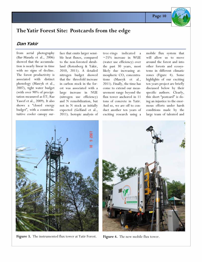
At the dawn of the new Millennium, in early 2000, we decided to setup a flux station site that will provide information on forest activities at the semi-a r i d ‘ d r y t i m b e r -line’ (Figure 1), which was not covered by the exten-sive efforts of the young Fluxnet. The only funding opportunity available was for a regular “large-equipment” grant as done when requesting a new microscope. This was not inappropriate: in adopting the flux tower as our re-search tool, we essentially ‘inverted the microscope’. We shifted from a reduc-tionist approach of trying to understand an organism by breaking it apart, to a holistic approach trying to understand how the parts integrate to explain the functioning of the Ecosys-tem. In reality, one cannot put up a flux site for the price of a microscope. And so, to make ends meet, we set out to a large junkyard. A set of sections of an old building construction crane was found that had the po-tential, with some imagina-tion, to form a tower at the right height and stability and at a bargain price (Figure 2). These were shipped to a friendly ma-chine shop, cleaned up,

The Yatir Forest Site: Postcards from the edge Dan Yakir

bottom of a 3x3x3 m hole and fixed, for ever, with the help of 11 tons of con-crete, at the center of the largest (~20,000 ha) and driest (290 mm precipita-tion) 40 year old pine for-

added the scientific coating onto the tower, and before long a state of the art flux tower began its operation (Figure 3). Being a field research site, not just a monitoring station, stu-

Figures 1&2. Yatir Forest (above) and an old building construction crane converted to a flux tower (below).

Page 10

face that emits larger sensi-ble heat fluxes, compared to the non-forested shrub-land (Rotenberg & Yakir, 2010, 2011). A detailed nitrogen budget showed that the threefold increase in carbon stock in the for-est was associated with a large increase in NUE (nitrogen use efficiency) and N remobilization, but not in N stock as initially expected (Gelfand et al., 2011). Isotopic analysis of

tree-rings indicated a ~25% increase in WUE (water use efficiency) over the past 30 years, most likely due increasing at-mospheric CO2 concentra-tions (Maseyk et al., 2011). Finally, the time has come to extend our meas-urement range beyond the flux tower anchored in 11 tons of concrete in Yatir. And so, we are off to con-duct another ten years of exciting research using a

mobile flux system that will allow us to move around the forest and into other forests and ecosys-tems in different climatic zones (Figure 4). Some highlights of our exciting ten years project are briefly discussed below by their specific authors. Clearly, this short “postcard” is do-ing an injustice to the enor-mous efforts under harsh conditions made by the large team of talented and

from aerial photography (Bar-Masada et al., 2006) showed that the accumula-tion is nearly linear in time with no signs of decline. The forest productivity is associated with distinct phenology (Maseyk et al., 2007), tight water budget (with over 90% of precipi-tation measured as ET; Raz Yaseef et al., 2009). It also shows a “closed energy budget”, with a counterin-tuitive cooler canopy sur-


Figure 3. The instrumented flux tower at Yatir Forest. Figure 4. The new mobile flux tower.

Page 11

Maseyk K, Grünzweig J, Rotenberg E and Yakir D (2008) Respiration accli-mation contributes to high carbon-use efficiency in a seasonally dry pine forest. Global Change Biology, doi: 1 0 . 1 1 1 1 / j . 1 3 6 5 -2486.2008.01604.x

Rotenberg E and Yakir D (2011) Distinct long- and short-wave radiation re-gimes in high productivity semi-arid pine forest. Glob-al Change Biology. 17, 1 5 3 6 - 1 5 4 8 . D o i : 1 0 . 1 1 1 1 / j / 1 3 6 5 -2486.2010.02320.x

Rotenberg R and Yakir D (2010) Contribution of semi-arid forests to the climate system. Science, 327, 451-454 DOI: 10.1126/science.1179998.

Maseyk K, Angert A, Hemming D, Leavitt S and Yakir D (2011) The con-trol of temperature and precipitation and CO2 on tree growth and water use efficiency in semi-arid woodland. Oecologia, 167, 5 7 3 - 5 8 5 . Doi:10.1007/s00442-011-2010-4.

Gelfand I, Grunzweig JM and Yakir D (2011) Slow-ing of nitrogen cycling and increasing nitrogen use efficiency following affor-estation of semi-arid shrub-

land. Oecologia, DOI 10.1007/s00442-011-2111-0

Raz-Yaseef N, Yakir D, Rotenberg E, Schiller G, Cohen S (2009) Ecohydrol-ogy of a semi-arid forest: partitioning among water balance components. Eco-h y d r o l o g y , D O I : 10.1002/eco.65

Contact:

Dan Yakir Department of Environ-mental Sciences and Energy Research Weizmann Insti-t u t e o f S c i e n c e Rehovot 76100 ISRAEL Tel: 972-8-934-2549 [email protected]

dedicated students and sci-entists, but we hope it will serve as an invitation to read more of the results from one of the most re-mote and unique Fluxnet sites.

References:

Grünzweig JM, Lin T, Rotenberg E and Yakir D ( 2 0 0 2 ) C a r b o n sequestration potential in arid-land forest. Global Global Change Biology, 9,791-799.

Bar Massada A, Carmel Y., Even Tzur G., Grünzweig JM, and Yakir D (2006) Assessment of temporal changes in above-ground forest tree biomass using aerial photographs and al-lometric equations. Canadi-an J Forest Res. 10, 2585-2594.

Grunzweig JM, Gelfand I and Yakir D (2007) Bioge-ochemical factors contrib-uting to enhanced carbon storage following afforesta-tion of semi-arid shrub-land. Biogeochemistry 4, 891-904.

Maseyk K, Tongbao L, Rotenberg E, Grünzweig J, Schwartz A and Yakir D (2007) Physiology phenol-ogy interactions in a pro-ductive semi-arid pine for-est. New Phytology, 178, 603-616.


Page 12

ation budget in semiarid regions in the 1970s postu-lated that “..reduction of vegetation, with conse-quent increase of albedo in the Sahel region would cause sinking (air) motion, additional drying, and would therefore perpetuate t h e a r i d c o n d i -tions…” (Charney, 1975; 1977 More recently, with greater awareness of the importance of the CO2 rise in the atmosphere, the con-trasting effects of vegeta-tion in removing atmos-

pheric carbon reducing its warming effect, while also decreasing surface albedo, enhancing surface warm-ing. But detail studies gen-erally focused on relatively wet regions (temperate, tropical). These aspects motivated us to link geo-physical (energy fluxes) and biogeochemical (carbon fluxes) studies in the Yatir forest to explore the po-tential for and implications of afforestation and deserti-fication in semi-arid re-gions (Rotenberg & Yakir,

2010, 2011). Both remote sensing (MODIS) and local meas-urements indicate that the forest canopy surface tem-perature in Yatir is lower than the surface tempera-ture in adjacent non-forested areas. While some surface cooling due to add-ed forest cover may sound reasonable, this finding is counter to expectations in Yatir for the following rea-sons. First, the forest albe-do is 0.1 lower than the surrounding, translating

With annual incoming solar radiation of ~7.5 GJ m-2 (~238 W m-2), the Yatir forest is exposed to a radiation load similar to that at the heart of the Sa-hara desert. Clearly, an evergreen forest needs to develop means to cope with such energy inputs, and with limited water availability this cannot be through the common evap-otranspiration route. Fur-thermore, Charney, who carried out pioneering studies on the surface radi-

The Yatir Forest Site: Solving the energy dissipation riddle in Yatir Eyal Rotenberg

Figure 1. Changes in surface energy fluxes associated with desertification (left; the Charney effect) and afforestation (right, the “Yatir effect). Upward and downward arrows indicate expected enhancement or suppression in flux asso-ciated with the land cover change.

Page 13

into a 24 W m-2 increase in radiation absorption by the forest canopy. Second, the forest “skin” surface (canopy and soil surface) is cooler, by 5˚C on annual mean.. Cooler surface emits less long-wave ther-mal radiation, and addi-tional 25 W m-2 are held back by the forest. Com-bined, the increased ab-sorption and reduced emis-sion, translate tothe nearly 50 W m-2 increase in radia-tion load associated with afforestation in this region. For comparison, this is as large as the difference in net radiation between, the Sahara desert and Den-mark, for example. Moreo-ver, latent heat flux, the common cooling and ener-gy dissipation mechanism in temperate forests, is not an option where water is virtually unavailable for some 7 months a year. And so, we are left with sensi-ble heat flux as the only major heat dissipation route. But sensible heat fluxes are normally directly proportional to the surface temperature, and our for-est surface is cooler… As it turned out sensible heat flux is indeed the major heat dissipation route. So much so that in summer the Bowen ratio (the ratio of sensible to latent heat fluxes), which is often


Figure 2: The radiation measurement setup over the Yatir forest, included: 2 - Kipp& Zonen CM21 for the solar radiation range, 2 - Eppley PIR for the thermal range,2 - Kipp&Zonen PQS1 for the PAR and 2 - Skye 4 Channel SKR 1850 sensors. A set of sen-sors is looking upward (to the atmosphere) the other downward.

Figure 3. Forest vs background and the characteristic mean annual values of energy flux-es above the semi-arid Yatir forest, compared to global mean values (in brackets). Note the high incoming short wave solar radiations (SWR) and low albedo (ratio of out-going to incoming SWR), the low latent heat (LE) and large sensible heat (H) fluxes.

Page 14

Charney, J. (1975). "Dynamics of deserts and drought in the Sahel." Quarterly journal of the Royal Meteorological Soci-ety 101(428): 193-202. Charney, J., W. J. Quirk, e t a l . ( 1 9 7 7 ) . "Comparative-Study of Effects of Albedo Change on Drought in Semi-Arid Regions." Journal of the Atmospheric Sciences 34(9): 1366-1385. Rotenberg, E. and D. Ya-kir (2010). "Contribution of Semi-Arid Forests to the Climate System." Science 327(5964): 451-454.

Contact:

Eyal Rotenberg Department of Environ-mental Sciences and Energy Research Weizmann Insti-t u t e o f S c i e n c e Rehovot 76100 ISRAEL Tel: 972-8-934-2549 eyal.rotenberg@weiz mann ac.il

around 1 in temperate for-ests, goes beyond 20 in Yatir, when the entire net solar radiation flux of ~800 W m-2 is dissipated as large sensible heat flux of the same magnitude. The solu-tion to this apparent “riddle” is simple when we recall that while sensible heat flux is indeed directly proportional to the surface temperature, but inversely proportional to the aerody-namic resistance of the sur-face layer. And a semi-arid forest with its low tree density and large surface area becomes an efficient low resistance “convector” well coupled to the sur-rounding atmosphere. In Yatir, the ‘canopy convec-tor effect’ is so efficient that the sensible heat flux is even greater than in the Sahara desert. It of course remains to be tested what are the consequences of the massive sensible heat fluxes above a sufficiently large forest area for the local circulation and synoptic systems. The Yatir forest is too small for that, but a modeling exercise is under way to address such ques-tions now that we have quantified the surface be-havior.

References


Page 15

Pushing a forest to the edge, like the case for the Yatir Forest, can provide insights into the responses and strategies that can be produced in response to climate change. This in-cludes changes in the tim-ing of individual life-cycle events (phenophases), which represent adapta-tions to maximise fitness in a particular environment.

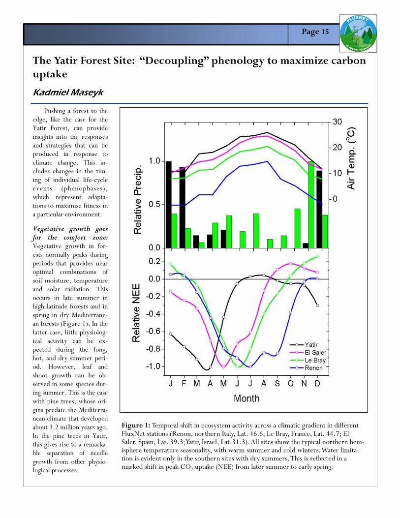
Vegetative growth goes for the comfort zone: Vegetative growth in for-ests normally peaks during periods that provides near optimal combinations of soil moisture, temperature and solar radiation. This occurs in late summer in high latitude forests and in spring in dry Mediterrane-an forests (Figure 1). In the latter case, little physiolog-ical activity can be ex-pected during the long, hot, and dry summer peri-od. However, leaf and shoot growth can be ob-served in some species dur-ing summer. This is the case with pine trees, whose ori-gins predate the Mediterra-nean climate that developed about 3.2 million years ago. In the pine trees in Yatir, this gives rise to a remarka-ble separation of needle growth from other physio-logical processes.

The Yatir Forest Site: “Decoupling” phenology to maximize carbon uptake

Kadmiel Maseyk

Figure 1: Temporal shift in ecosystem activity across a climatic gradient in different FluxNet stations (Renon, northern Italy, Lat. 46.6; Le Bray, France, Lat. 44.7; El Saler, Spain, Lat. 39.3; Yatir, Israel, Lat.31.3). All sites show the typical northern hem-isphere temperature seasonality, with warm summer and cold winters. Water limita-tion is evident only in the southern sites with dry summers. This is reflected in a marked shift in peak CO2 uptake (NEE) from later summer to early spring.

Page 16

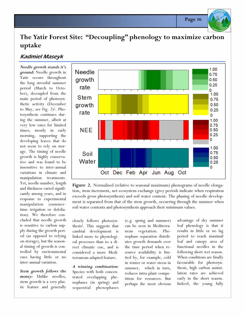
Needle growth stands it’s ground: Needle growth in Yatir occurs throughout the long stressful summer period (March to Octo-ber), decoupled from the main period of photosyn-thetic activity (December to May, see Fig. 2)2. Pho-tosynthesis continues dur-ing the summer, albeit at very low rates for limited times, mostly in early morning, supporting the developing leaves that do not seem to rely on stor-age. The timing of needle growth is highly conserva-tive and was found to be insensitive to inter-annual variations in climate and manipulation treatments. Yet, needle number, length and thickness varied signifi-cantly among years, and in response to experimental manipulation (summer-time irrigation or defolia-tion). We therefore con-cluded that needle growth is sensitive to carbon sup-ply during the growth peri-od (as opposed to relying on storage), but the season-al timing of growth is con-trolled by environmental cues having little or no inter-annual variation.

Stem growth follows the money: Unlike needles, stem growth is a very plas-tic feature and generally


Kadmiel Maseyk

Figure 2. Normalised (relative to seasonal maximum) phenograms of needle elonga-tion, stem increment, net ecosystem exchange (grey periods indicate when respiration exceeds gross photosynthesis) and soil water content. The phasing of needle develop-ment is separated from that of the stem growth, occurring through the summer when soil water contents and photosynthesis approach their minimum values.

closely follows photosyn-thesis3. This suggests that cambial development is linked more to physiologi-cal processes than to a di-rect climatic cue, and is considered a more Medi-terranean-adapted feature.

A winning combination: Species with both concen-trated overlapping phe-nophases (in spring) and sequential phenophases

(e.g. spring and summer) can be seen in Mediterra-nean vegetation. Phe-nophase separation distrib-utes growth demands over the time period when re-source availability is lim-ited by, for example, cold in winter or water stress in summer, which in turn, reduces intra-plant compe-tition for resources. But perhaps the most obvious

advantage of dry summer leaf phenology is that it results in little or no lag period to reach maximal leaf and canopy area of functional needles in the following short wet season. When conditions are finally favourable for photosyn-thesis, high carbon assimi-lation rates are achieved early in the short season. Indeed, the young fully

Page 17

expanded needles show the highest rates of assimilation at that time among the leaf cohorts. Achieving this high early season capacity is also supported by high leaf nitrogen contents at the start of the season due to the completion of growth-related N remobilisation and translocation (see sec-tion on Nitrogen in this Letter), and other adjust-ments to the semi-arid con-ditions including dynamic pigmentation to protect needles from photo-damage (reduction in chlo-rophyll and increase xan-thophyll cycle pigments). Having canopy develop-ment during the hydrologi-cal limitation period also helps maintain canopy size at sustainable levels. These results highlight important features when considering functional re-sponses to environmental change: the response across phenological processes of a species will differ, depend-ing on the nature of the change, the drivers of the phenophases and evolution-ary constraints on plastici-ty. It appears that the sepa-ration of wood and foliage phenophases in this dry environment enables more efficient allocation of re-sources, optimizes canopy development and maximiz-


Kadmiel Maseyk

es carbon gain. Some in-vestment is required, how-ever, in mechanisms pre-venting photo-oxidative damage and hydrological stress to maintain dry sea-son leaf phenology. Under-standing the interactions between climate, physiolo-gy and phenology in this system provides insights into features contributing to the success of pines un-der warm and dry condi-tions, and may have more general relevance to (warming and drying) tem-perate regions as well.

References

Orshan, G. Plant Pheno-morphological Studies in Mediterranean Type Eco-systems. Vol. 12 (Kluwer Academic Publishers, 1989).

Maseyk, K. S. et al. Physi-ology-phenology interac-tions in a productive semi-arid pine forest. New Phy-tologist 178, 603-616, d o i : 1 0 . 1 1 1 1 / j . 1 4 6 9 -8 1 3 7 . 2 0 0 8 . 0 2 3 9 1 . x (2008).

Maseyk, K., Grunzweig, J. M., Rotenberg, E. & Ya-kir, D. Respiration accli-mation contributes to high carbon-use efficiency in a

seasonally dry pine forest. Global Change Biology 14, 1553-1567, doi:10.1111/j.1365-2486.2008.01604.x (2008).

Liphschitz, N. & Lev-Yadun, S. Cambial Activity of Evergreen and Seasonal Dimorphics around the Mediterranean. Iawa Bulle-tin 7, 145-153 (1986).

Contact:

Kadmiel Maseyk K a d m i e l . M a s e y k @ g r i g non.inra.fr

Page 18

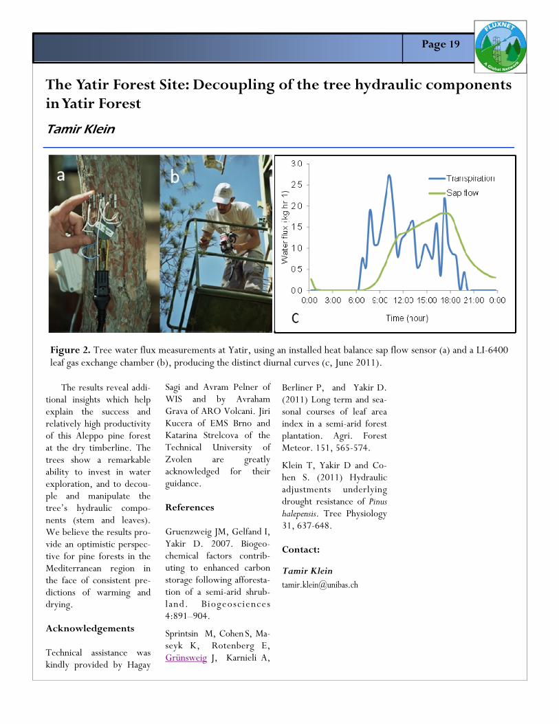
Investment in explora-tion: When water is scarce, more resources need to be devoted to-wards exploring for it and extracting it from the soil. This is clearly seen in Pinus halepensis, the dominant tree species in Yatir. In-creasing water stress trig-gers dramatic shifts in bio-mass allocation among leaves, stems, and roots. While in the absence of water stress total root growth is only 34% of freshly synthesized bio-mass, it increases to as high as 87% under severe water stress conditions (Figure 1; see Klein et al., 2011 for details). The in and the out of tree water use: Tree wa-ter use is often estimated by tree-scale stem sap flow, or by short-term leaf-scale gas exchange meas-urements. We applied both methods simultaneously, and scaled up both meas-urements to the stand level by relying on extensive estimates of LAI and local, site-specific allometric equations (Gruenzweig et al., 2007; Sprintsin et al., 2011). As expected, on the daily time-scale, water mass balance exists be-tween the trunk and the

The Yatir Forest Site: Decoupling of the tree hydraulic components in Yatir Forest

Tamir Klein

leaves. On shorter time-scales, however, strong decoupling between stem sap flow and leaf transpira-tion was observed (Figure 2). Examining the diurnal dynamics showed that changes in sap flow are gradual, while transpiration rates greatly fluctuate, and peak transpiration can be twice that of sap-flow; Moreover, we found that transpiration ceases at night, whereas sap flow continued long after dark. The hazards and safe-guards of decoupling: The relative magnitude of nocturnal sap flow during summer months surpasses some previously reported values for pine forests. The observations that sap flow occurred at night, tempo-rally decoupled from leaf transpiration, imply that the tree xylem undergoes substantial changes in its water content on a daily basis. Such changes may involve large short-term deficits of up to 15 dm3 of water per tree, although some of the xylem hydrau-lic imbalance may be buff-ered by short-term water storage capacity. Nonethe-less, the observed decou-pling must also mean the development of embolism

in xylem tracheids, as ob-served in the dynamics of the percent loss of hydrau-lic conductivity (PLC, up to 40%). This, in turn, would require a capacity to recover hydraulic conduct-ance to maintain the ob-served hydraulic patterns in

a continuous manner. In-deed our latest findings provide evidence on the capacity for rapid recovery from loss of hydraulic con-ductivity in Pinus halepensis (within a few hours and repeating twice in a single daytime cycle).

Figure 1. Partitioning of dry biomass accumulation among leaves, stems and roots of Pinus halepensis under conditions of increasing water stress.

Page 19

The results reveal addi-tional insights which help explain the success and relatively high productivity of this Aleppo pine forest at the dry timberline. The trees show a remarkable ability to invest in water exploration, and to decou-ple and manipulate the tree’s hydraulic compo-nents (stem and leaves). We believe the results pro-vide an optimistic perspec-tive for pine forests in the Mediterranean region in the face of consistent pre-dictions of warming and drying. Acknowledgements Technical assistance was kindly provided by Hagay

The Yatir Forest Site: Decoupling of the tree hydraulic components in Yatir Forest

Tamir Klein

Sagi and Avram Pelner of WIS and by Avraham Grava of ARO Volcani. Jiri Kucera of EMS Brno and Katarina Strelcova of the Technical University of Zvolen are greatly acknowledged for their guidance. References Gruenzweig JM, Gelfand I, Yakir D. 2007. Biogeo-chemical factors contrib-uting to enhanced carbon storage following afforesta-tion of a semi-arid shrub-land. Biogeosciences 4:891–904.

Sprintsin M, Cohen S, Ma-seyk K, Rotenberg E, Grünsweig J, Karnieli A,

Berliner P, and Yakir D. (2011) Long term and sea-sonal courses of leaf area index in a semi-arid forest plantation. Agri. Forest Meteor. 151, 565-574.

Klein T, Yakir D and Co-hen S. (2011) Hydraulic adjustments underlying drought resistance of Pinus halepensis. Tree Physiology 31, 637-648. Contact:

Tamir Klein [email protected]

Figure 2. Tree water flux measurements at Yatir, using an installed heat balance sap flow sensor (a) and a LI-6400 leaf gas exchange chamber (b), producing the distinct diurnal curves (c, June 2011).

Page 20

Puzzlement motivated research: The survival and success of the Yatir forest is a puzzle. Average precipi-tation is 283±88 mm yr-1, but drought years occur regularly, and precipitation as low as 138 mm yr-1 has been recorded since the planting of the forest. The rainy season is short, lead-ing to seasonal droughts, with prolonged near-hygroscop-ic surface soil water content levels lasting through the long summer (~5% m3 m-3 from June to November). Groundwater is deep (~300 m), and be-cause soil water potentials are low, no deep drainage or uptake from depths be-low 2-3 m can be ex-pected. Yet, a relatively high productivity forest has been growing here over the past 45 years. Understand-ing the water dynamics within the forest is key to unraveling this puzzle, and helps predict the future of forests across the Mediter-ranean regions undergoing drying trends. A decade of field measurements and analysis has revealed a range of interesting and unexpected processes. Developments motivated by technological needs: First, we noted that the

afforestation essentially totally eliminated runoff. While impressive flash floods were observed at times in the surrounding shrubland, the runoff mon-itoring station at the exit of the Yatir forest watershed stays dry even during the strongest storms. Indeed,

measurements of evapo-transpiration (ET) show that, on average, ET ac-counts for 94% of annual precipitation (Fig. 1; Raz-Yaseef et al., 2010a). Next, our attention was drawn to soil evaporation (Es). In an open-canopy forest, exposed to high

radiation load, we ex-pected soil evaporation to be an important compo-nent requiring examina-tion. But reliable methods to directly measure soil evaporation at high spatial and temporal resolution were absent. This motivat-ed us to develop our own

The Yatir Forest Site: Ecohydrology of Yatir – a forest growing in the desert

Naama Raz-Yaseef

Figure 1. Components of the hydrological cycle in the Yatir forest: Precipitation (P), interception by the canopy (EI), through-fall (Pt), tree transpiration (ET), soil evapora-tion (ES), soil water adsorption (A), soil water storage (S). Losses (L) out of the system included runoff (Q), subsurface flow (F), deep drainage (D).

Page 21

method by modifying our standard soil respiration chambers and the measure-ment protocol. The effort was worthwhile. Results indicated that soil evapora-tion accounted for 39% of the total evaporative losses, with large spatial variabil-ity. Evaporation fluxes in open gaps were twice as high as those in shaded are-as. Simulating tree shading in our forest allowed us, in turn, to predict how the


Naama Raz-Yaseef

partitioning of ET would vary with changes in the forest tree density. This simple predictive tool indi-cated that current tree den-sity (300 trees ha-1, canopy cover of 54%), previously arrived at empirically by foresters, is in fact near optimal. Higher tree den-sity at this site would in-crease ET demands beyond the average precipitation input and could result in tree mortality. Reducing

tree density would result in greater losses to soil evapo-ration (Fig. 2; Raz-Yaseef et al., 2010b). Need to scratch the sur-face: The proportional contribution of different flux component to total ET varied seasonally, due to their differential response to seasonal environmental

drivers (Raz-Yaseef et al., 2012). Soil evaporation was correlated to soil mois-ture at the topsoil (0-10 cm). It peaked twice dur-ing the seasonal cycle: Once during the wetting period in the fall, and again during drying season in spring. These periods were characterized by superficial

Figure 2. Changes in the proportional contribution to the ecosystem hydrological balance as a function of canopy cover (forest tree density). Shading increases and soil evaporation decreases with increasing canopy cover, but increased interception and tree transpira-tion reduces residual (excess) water in the system. Excess water is the component available for runoff and recharge to depth or for additional vegetation. Under current precipitation (285 mm yr-1, dotted horizontal line) and tree density (65% cover, 300 tree ha-1) the system is nearly balanced.

Figure 3. Inter-annual variations: similar annual pre-cipitation but low intensities (2005/6) or high (based 2007/8) years produced significant differences in tree transpiration (Et). Only storms of >30 mm infiltrate below 20 cm soil depth and into the main root zone. Increasing storm intensity can compensate for reduced total precipitation.

Page 22

soil moisture and high radi-ation. Summer was too dry and winter was too cold to generate significant evapo-ration fluxes. Surprisingly, low evaporation fluxes were measured throughout the dry summer period. Perhaps even more surpris-ing was the conclusion that ~50% of the daily flux was due to re-evaporation of moisture condensed onto the soil at night (measured as negative water fluxes from atmosphere to the soil). In contrast to soil evaporation, tree transpira-tion (Tt) was associated with soil moisture at a 10-20 cm depth layer (the depth of maximum root density), and peaked only in late spring (~1.5 mm d-

1), after the accumulation of moisture from the few larger storms that infiltrat-ed below the topsoil layer. Moisture at this depth was maintained for much long-er periods than at the sur-face, often with carry-over between hydrological years. Ultimately, the ratio Tt/ ET, the major link to forest productivity and survival, was more strongly associated with the fraction of precipitation from larger storm (>30 mm), than with total annual precipita-tion.


Naama Raz-Yaseef

These results are sig-nificant because climate change scenarios for the Mediterranean often pre-dict drying but also increas-ing storm intensity. Our findings indicate that the latter effect (intensity) can at least partially compen-sate for the former (drying) (Fig. 3). References Raz-Yaseef, N., Roten-berg, E., Yakir, D., 2010a. Effects of spatial variations in soil evaporation caused by tree shading on water flux partitioning in a semi-arid pine forest. Agricul-tural and Forest Meteorol-ogy 150 (3): 454-462. Raz-Yaseef, N., Yakir, D., Rotenberg, E., Schiller, G., Cohen, S., 2010b. Ecohydrology of a semi-arid forest: partitioning among water balance com-ponents and its implica-tions for predicted precipi-tation changes. Ecohydrol-ogy 3: 143-154. Raz Yaseef, N., Yakir, D., Schiller, G., Cohen, S., 2012. Dynamics of evapo-transpiration partitioning in a semi-arid forest as affect-ed by temporal rainfall pat-terns. Agricultural and

Forest Meteorology 157, 77-85. Contact:

Naama Raz-Yaseef Climate and Carbon Sci-ences Program, Earth Sci-ences Division, Lawrence Berkeley National Labora-t o r y , B e r k e l e y , C A . [email protected]

Page 23

Ecosystems in dry re-gions are generally low in productivity and carbon storage, but the Yatir for-est seems to defy such as-sumptions. This was checked quantitatively by eddy covariance measure-ments over 10 years. But, eddy flux measurements have their own difficulties and uncertainties and must be backed up and con-strained by additional measurements, and ulti-mately by “carbon account-ing”.

Carbon stocks meet car-bon fluxes: Much effort was invested in Yatir to add this perspective, by aerial photography (Bar Massada et al., 2006), and by esti-mating carbon stocks both below and above ground. As it turned out, planting a Pinus halepensis forest in an overgrazed, semi-arid shrubland increased the soil organic carbon stock by 75% over a period of 35 years (Grünzweig et al., 2007). Adding the tree and understory carbon invento-ry (using site-specific al-lometric equations; See Figure 1) to soil organic carbon, obtained by cor-ing, produced estimates of the ecosystem carbon stock. In total, those in

The Yatir Forest Site: Backing up the flux measurements in the Yatir Forest

José M. Grünzweig

the forest were 2.5 fold the carbon stock in the shrub-land. Aerial photography suggests a near linear in-crease in aboveground tree carbon stock over time (Bar Massada et al., 2006), which allowed us to esti-mate meaningful average annual increases of 180 g C m−2 yr−1 over 35 years. These estimates are con-sistent with the recent NEE measurements of just over 200 g C m−2 yr−1 with large inter-annual variations (Grünzweig et al., 2003; Rotenberg & Yakir, 2010).

No nutrients to the res-cue: Such a large increase in carbon stocks would suggest the need for a simi-lar increase in nutrient stocks, mainly nitrogen. However, nitrogen stocks did not change significantly due to afforestation. Con-sequently, the ecosystem C/N ratio increased mark-edly from 7.6 in the native shrubland to 16.6 in the forest, suggesting an in-crease in nitrogen use effi-ciency by the ecosystem (Grünzweig et al., 2007).

No water and no decom-position: Biogeochemical mechanisms enabling the rise in carbon storage in-clude low decomposition rates due to recalcitrant pine litter and dry condi-tions (the volumetric water content of the upper 40 cm of the soil profile is below 20% over 75% of the year and below 12% over 65% of the year). 13C isotopic analyses indicated a small isotopic signal introduced by relatively 13C-rich pine biomass (-23 to -24‰) as compared to 13C-poor

Figure 1. Subsampling stem sections and branches for moisture content during a field campaign aimed at creating site-specific allometric equations for Pinus halepensis (picture courtesy: Avi Bar Masada).

Page 24

shrubland vegetation (-26 to -29‰), leading to a dis-tinct pine signal especially in the litter and the upper soil layers (Figure 2). This helped us to show that soil organic matter (SOM) de-rived from pine inputs de-cays at low rates, likely as a consequence of protection within organo-mineral complexes. Low decay rates of litter and SOM were also confirmed by relat ively low soil-respiration rates as deter-

The Yatir Forest Site: Backing up the flux measurements in the Yatir Forest

José M. Grünzweig

mined by measurements of CO2 efflux from the soil surface (Grünzweig et al., 2009). And, soil respira-tion rates were low despite high root production (Grünzweig et al., 2007), and relatively high below-ground NPP (root produc-tion, exudation, micorrhiza etc.; Gelfand et al., 2012) and belowground carbon allocation (~40% of GPP; Grünzweig et al., 2009). Therefore, in the light of the total carbon budget, we

concluded that the high carbon sequestration of the Yatir semi-arid pine forest reflects its relatively high productivity, moderate nitrogen requirements and low heterotrophic carbon loss rates.

References

Bar Massada A, Carmel Y., Even Tzur G., Grünzweig JM and Yakir D (2006) Assessment of temporal changes in aboveground forest tree biomass using aerial photographs and al-lometric equations. Cana-dian Journal of Forest Re-search 10, 2585-2594. Gelfand I, Grünzweig JM and Yakir D (2012) Slow-ing of nitrogen cycling and increasing nitrogen use efficiency following affor-estation of semi-arid shrub-land. Oecologia, 168, 563-575. doi: 10.1007/s00442-011-2111-0 Grünzweig JM, Lin T, Ro-tenberg E, Schwartz A and Yakir D (2003) Carbon sequestration in arid-land forest. Global Change Biol-ogy 9,791-799.

Grünzweig JM, Gelfand I, Fried Y and Yakir D (2007) Biogeochemical factors contributing to enhanced

carbon storage following afforestation of a semi-arid shrubland. Biogeosciences 4 , 8 9 1 - 9 0 4 . d o i : 1 0 . 5194/bg-4-891-2007

Grünzweig JM, Maseyk K, Hemming D, Lin T, Ro-tenberg E, Faloon and Ya-kir D (2009) Water limita-tion to soil CO2 efflux in a pine forest at the semi-arid ‘timberline’. Journal of Geophysical Research 114, G 0 3 0 0 8 , d o i : 10.1029/2008JG000874.

Rotenberg E and Yakir D (2010) Contribution of semi-arid forests to the climate system. Science 327, 451-454 do i : 10.1126/science.1179998. Contact: José M. Grünzweig j o s e . g r u e n z w e i g @ mail.huji.ac.il

Figure 2. Small isotopic signal of pine biomass record-ed throughout the litter layer (0 cm depth) and soil profile (0-50 cm depth). This relatively 13C-rich signal allowed us to calculate the addition of new organic car-bon and of decay of old shrubland-derived carbon in the soil (from Grünzweig et al., 2007).

Page 25

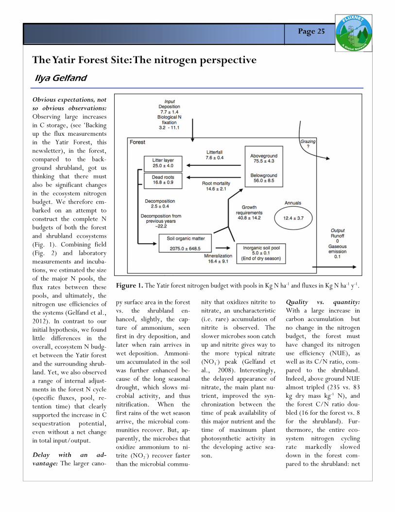
Obvious expectations, not so obvious observations: Observing large increases in C storage, (see ‘Backing up the flux measurements in the Yatir Forest, this newsletter), in the forest, compared to the back-ground shrubland, got us thinking that there must also be significant changes in the ecosystem nitrogen budget. We therefore em-barked on an attempt to construct the complete N budgets of both the forest and shrubland ecosystems (Fig. 1). Combining field (Fig. 2) and laboratory measurements and incuba-tions, we estimated the size of the major N pools, the flux rates between these pools, and ultimately, the nitrogen use efficiencies of the systems (Gelfand et al., 2012). In contrast to our initial hypothesis, we found little differences in the overall, ecosystem N budg-et between the Yatir forest and the surrounding shrub-land. Yet, we also observed a range of internal adjust-ments in the forest N cycle (specific fluxes, pool, re-tention time) that clearly supported the increase in C sequestration potential, even without a net change in total input/output.

Delay with an ad-vantage: The larger cano-

The Yatir Forest Site: The nitrogen perspective

Ilya Gelfand

py surface area in the forest vs. the shrubland en-hanced, slightly, the cap-ture of ammonium, seen first in dry deposition, and later when rain arrives in wet deposition. Ammoni-um accumulated in the soil was further enhanced be-cause of the long seasonal drought, which slows mi-crobial activity, and thus nitrification. When the first rains of the wet season arrive, the microbial com-munities recover. But, ap-parently, the microbes that oxidize ammonium to ni-trite (NO2

-) recover faster than the microbial commu-

nity that oxidizes nitrite to nitrate, an uncharacteristic (i.e. rare) accumulation of nitrite is observed. The slower microbes soon catch up and nitrite gives way to the more typical nitrate (NO3

-) peak (Gelfand et al., 2008). Interestingly, the delayed appearance of nitrate, the main plant nu-trient, improved the syn-chronization between the time of peak availability of this major nutrient and the time of maximum plant photosynthetic activity in the developing active sea-son.

Quality vs. quantity: With a large increase in carbon accumulation but no change in the nitrogen budget, the forest must have changed its nitrogen use efficiency (NUE), as well as its C/N ratio, com-pared to the shrubland. Indeed, above ground NUE almost tripled (235 vs. 83 kg dry mass kg-1 N), and the forest C/N ratio dou-bled (16 for the forest vs. 8 for the shrubland). Fur-thermore, the entire eco-system nitrogen cycling rate markedly slowed down in the forest com-pared to the shrubland: net

Figure 1. The Yatir forest nitrogen budget with pools in Kg N ha-1 and fluxes in Kg N ha-1 y-1.

Page 26

N mineralization rates in the soil decreased by ap-proximately 50%, decom-position rates decreased by approximately 20%, and a decrease of approximately 64% in NOx loss in volati-lazation was estimated (Glefand et al., 2009). While our investiga-tion was by no means ex-haustive, the first insights into the N cycle of a pine forest at the dry timberline provide another piece of the puzzle that help explain the observed 2.5-fold in-crease in the C stock of this ecosystem without the need to invoke any signifi-cant changes in the N stocks.

References

Gelfand I and Yakir D (2008) Influence of nitrite accumulation in association with seasonal patterns and mineralization of soil nitro-gen in a semi-arid pine for-est. Soil Biology Bio-chemi, 40, 415-424. Gelfand, I, Feig, G, Meixner FX, Yakir D (2008) Effects of semi-arid shrubland afforestation on biogenic NO emission from soil. Soil Biology Biochemi, 41, 1561-1570. Gelfand I, Grunzweig JM and Yakir D (2012) Slow-ing of nitrogen cycling and

The Yatir Forest Site: The nitrogen perspective

Ilya Gelfand

increasing nitrogen use efficiency following affor-estation of semi-arid shrub-land. Oecologia, 168, 563-575. DOI 10.1007/s00442-011-2111-0 Contact Ilya Gelfand W.K. Kellogg Biological Station, Michigan State University 3700 E Gull Lake Dr Hickory Corners, Mi 49060 [email protected]

Figure 1. The Yatir forest nitrogen budget with pools in Kg N ha-1 and fluxes in Kg N ha-1 y-1.

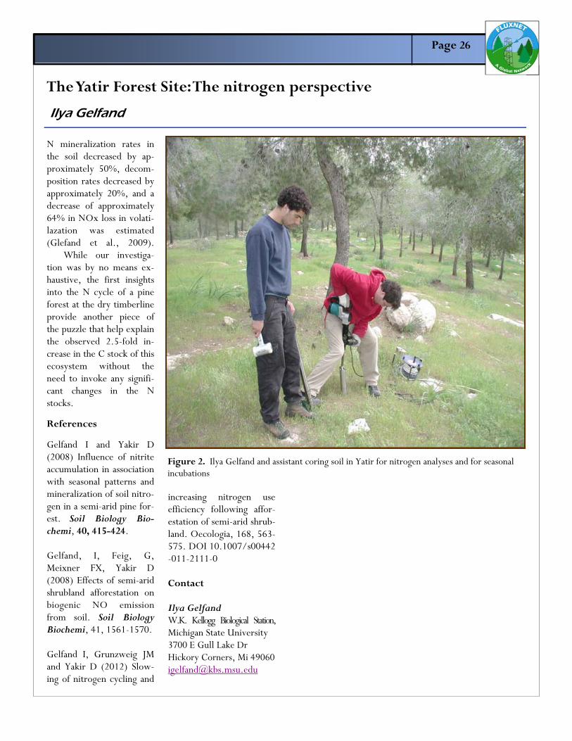
Figure 2. Ilya Gelfand and assistant coring soil in Yatir for nitrogen analyses and for seasonal incubations

Page 27

This past Septem-ber, Prof. Shashi Ver-ma retired from the University of Nebraska, Lincoln after a career that spanned the years 1974 to 2012. We want to take this op-portunity to profile, Prof. Verma, in the Fluxletter, and remi-nisce on his many con-tributions to our field. Shashi Verma is one of the pioneers of mak-ing eddy covariance measurements of CO2 and water vapor fluxes between vegetation and the atmosphere. He was a mentor to many of us active in the FLUXNET community (e.g. Joon Kim, George Burba, Dean Anderson, and this author). And his developments and findings were funda-mental in founding and execu t ing long- te rm f l u x m e a s u r e m e n t s across regional and global networks. I first met Prof. Verma early one morn-

A Tribute to Shashi Verma

Dennis Baldocchi

ing (by early I mean 5 am), August, 1977. I had just arrived in Lin-coln, Nebraska to start graduate work under the tutelage of Prof. N o r m R o s e n b e r g , whom we affectionately called ‘Doc’. I was told to arrive at the lab early to join the crew on the daily trip to Mead for field re-search, and to help move irrigation pipe. Having just fled our California walnut farm, where I had been mov-ing irrigation pipe daily for over a decade, I was hoping for better and greater tasks. That morning, as I peered into the truck I saw this young guy—he was a few years over 30, the age of many post-docs—an assistant pro-fessor named Shashi Verma. ‘Who is this guy?’, I thought, as I had expected Doc. I soon found out who this guy was. He proved to me to be a b r i l l i an t , i n s i gh t fu l , patient, kind, hard-working and innovative scientist. What I did not an-ticipate at the time was how he was on the verge of pushing the fields of agricultural meteorology and bio-meteorology so far for-

ward. At this time, the f ield of agricultural meteorology was focus-ing on measuring crop temperature with infra-red thermometers and relating these tempera-tures to crop stress and yield. Shashi was trained as a civil engi-neer (BS, Ranchi Uni-vers i ty , Ind ia ; MS, University of Colora-do; PhD, Colorado State University) and was on the verge of bringing his engineer-ing training to agricul-ture. He knew it was the flux of heat and matter that controls the local environment and affects water use and primary productiv-ity. So, Shashi was fixed on developing the new eddy covariance method to measure these fluxes directly. This desire led him to work with scientists at Lawrence L ivermore Nat iona l Lab (Ga i l Bingham) to develop and deploy a new open-path CO2 sensor to measure crop photo-synthesis. He was also at the vanguard by us-ing computers to col-lect data on magnetic tape. This was a big deal at the time, as the ub iqu i tous Campbel l data-loggers had not been developed, yet.

( R o s e n b e r g ’ s d a t a -logger was a DATEX; a huge analog device that punched holes in paper tape to record voltages of solar radiation, tem-perature and humidity. If the paper tape tore you could tape it to-gether. Over the course of the next five years Shashi and his students would produce some of the first eddy covari-ance measurements of carbon dioxide and wa-ter vapor flux over crops, like soybeans and sorghum. In the meantime, he was also a pioneer in conducting comparative flux meas-urements; a way of us-ing micrometeorology flux measurement tech-nology to ask and an-swer scientific ques-tions. In the early 1980’s he had a project working with geneti-cists to develop better crops to feed the world. One idea in-volved changing the morphology of soy-beans -- to examine how creating soybeans with hairy and narrow leaves affected their mass and energy ex-change. By measuring fluxes over two com-parative fields simulta-neously, Verma was able to deduce impacts

Page 28

of these morphological changes relative to co-occurring weather. After my cohort graduated, Shashi start-ed down a new path of research on methane fluxes, with the new Campbell tunable diode l a s e r s p e c t r o m e t e r . With his student Joon K im and co l l e ague Dave Billesbach, Verma and company made some of the first season long, eddy covariance flux measurements of methane in harsh wet-land environments in M i n n e s o t a , w e s t e r n Nebraska and Saskatch-ewan, Canada. One of the great things about Shashi as a mentor is that you could go to his office and ask any question any time about any-thing science related. I don’t recall ever being rebuked, or ever hav-ing left his office with-out the answer. An-other great thing about his mentorship is that he gave his students the resources to do the work. Maybe it was a different time, but we never worried about funding or instrumen-tation to do the work or go to meetings to present the work. He also taught us how to be careful scientists

Tribute to Shashi Verma

Dennis Baldocchi and the importance of calibration—the man-tra in my lab today is ‘ca l ibra te, ca l ibra te, calibrate’. In those early days he’d cali-brate the eddy covari-ance system every 3 hours. He’d zero the psychrometer system hourly, and he had us go through every line of computer code and repeat the calculations by hand to make sure the code was correct in computing fluxes! And when it came to writ-ing up the work, he was there with con-s t r u c t i v e c r i t i c i s m . Not being the best writer, my manuscripts would come back all red, with suggestions for improvements, bet-ter ways to think about the sentences and the material we were pre-senting. On leaving Nebras-ka, I had many oppor-tunities to continue working with Shashi. In 1984, he came to Oak Ridge with his ‘new fangled’ CO2 sensor and we made the first measurements of CO2 exchange over a deciduous forest. That work was so new that we produced 5 peer reviewed papers with 3 weeks o f me asure -m e n t s . O u r n e x t

chance to collaborate was in 1993-94 in Can-ada during the BOREAS experiment. Later in our careers we had the pleasure of meeting at least once a year at sci-entific meetings, like Ameriflux or the AMS AgForest Met confer-ence. Then, we had much fun sitting to-gether, visiting, going to dinner and talking about life in general, family and science. Shashi Verma is a modest individual, who has had a distinguished career. Among his honors, he is a fellow of the Agronomy Socie-ty of America, recipi-ent of the American Meteoro logy Soc ie ty Award for Outstanding Achievement in Biome-teorology and Charles Bessey Professor of Natural Resources. In closing, I’d like to remark on his scien-tific pedigree. He was a student of the late Jack Cermak, an engi-neer at Colorado State University, who was noted for wind tunnel studies of wind flow in urban settings. What I did not know about was w h o h i s s c i e n t i f i c grandfather and great g r a n d f a t h e r w e r e . During the BOREAS p r o j e c t , w h e r e w e

worked together again in Canada, I was sitting in the Toronto airport waiting for a flight home. Wilf Brutsaert, the engineering profes-sor at Cornell, known for his book on Evapo-ration, walked up to me and said: ‘you are Shashi Verma’s stu-dent….you are related to Ted von Karman, two degrees removed’, and walked away; von Karman was the the fluid mechanics profes-sor at Cal Tech, best known for the von Kar-man constant (k = 0.40). I asked Shashi about this encounter and he could not verify this genealogy. More recently, I was at a meeting in Lausanne, Switzerland and sat next to Prof. Brutsaert on the bus to a field trip, so I asked him about this genealogy. He said Bill Sears was a student of von Karman. Jack Cermak was a stu-dent of Sears at Cor-nell, followed by Ver-ma. So in closing, we thank you for your con-tributions to science and your fine mentor-ing and we wish you a happy and healthy re-tirement and much fun and time with your son and his family in Texas.

Page 29

The ‘Sunset’ neigbor-hood in Vancouver, BC, may be the most extensive-ly studied area in urban climatology. Since 1977, about 50 papers have been published that focus on flux measurements, land-atmosphere exchange, and models developed using data gathered on and around the ‘Vancouver-Sunset’ micrometeorologi-cal tower. This newsletter contribution aims to pro-vide a brief history of this unique flux tower, show how selected developments in urban climatology were linked to work at this site, and highlight some of the ongoing research on urban trace-gas flux measure-ments to validate fine-scale emission models.

Establishing an urban micrometeorological tower (1977) One of the biggest conceptual chal-lenges in urban climatology is the spatial heterogeneity of cities. From single lots (roofs, walls, streets, lawns) to the land-cover patchiness in an urban neighborhood (parks, low-density, high-density areas) up to the differences in surface properties between cities and the surrounding area (urban heat island, country breezes etc.) - ur-ban systems are dominated

by heterogeneity on many scales, and advection is the norm rather than the ex-ception. From the start it was clear that micromete-orological approaches and theories developed for flat and homogeneous sites would be unlikely to apply a priori to the study of ur-ban land-atmosphere inter-actions. Moreover, it is challenging to separate urban effects from other effects (local winds, land-cover differences, topogra-phy, synoptic effects) un-less proper experimental control (Lowry, 1977) has been established. In the 1960s and 1970s the mostly unpublished trials to measure turbulent fluxes above urban surfaces were flawed because mi-crometeorological methods were applied with instru-ments situated generally too close (low) to the ele-ments that constitute the urban surface e.g. on roof-tops or on small masts with-in the layer that is now recognized as the rough-ness sublayer (Raupach and Thom, 1981). In the 1970s, there was growing evidence from pioneering work such as the turbu-lence studies using eddy covariance (EC) instru-ments mounted on masts during METROMEX in St. Louis, USA (Clarke et al.,

1978) and in both Vancou-ver (Burnaby) and Uppsala by Oke (1978) that micro-meteorological methods might work as long as the measurement height was well above the height of the buildings. In other words, in the inertial sublayer

above extensive urban sur-faces where individual flow-distorting effects of build-ings are blended. Can fluxes be meas-ured successfully using tra-ditional micrometeorologi-cal approaches, if we are high enough above the sur-

35 years of urban climate research at the ‘Vancouver-Sunset’ flux tower

Andreas Christen, Tim Oke , Sue Grimmond , Douw Steyn and Matthias Roth

Figure 1. Then graduate student Douw Steyn (left) and research assistant Brian Guy (right) celebrating having fi-nally completed installation of the complete set of mast mounted instrumentation in July 1978. The set-up includ-ed a uvw propellor anemometer (top), a wind profile with cup-anemometers, a yaw-sphere and a Bowen-Ratio sys-tem (bottom right), all approaches adopted from work in agricultural and forest climatology.

Page 30

face? How high is high enough? What are site re-quirements that would al-low this? What would be an appropriate site in the complex setting of a city like Vancouver? Those questions were part of a graduate research seminar led by then Associate Pro-fessor Tim Oke at the Uni-versity of British Colum-bia, in the mid-1970s. As an exercise, students were involved in the identifica-tion of a ‘homogeneous’ site in Vancouver at which it would be possible to make successful microme-teorological measure-ments. The criteria devel-oped were: (a) no major changes in building and tree height and density around the site, (b) a rela-tively flat area, and (c) no significant land-cover boundaries (i.e. a sufficient fetch). One of the sites identified by his students, using maps and air photos was the ‘Sunset’ residential neighborhood. Follow-up work suggested it might be possible to erect a tower in this area, inside a power substation of BC Hydro, where security was good. Subsequently, after gaining the approval of the city planning authorities and the local residents and with funding from the Natural Science and Engineering



Research Council of Cana-d a ( N S E R C ) t h e ‘Vancouver Sunset’ tower was established in 1977 (123.0784ºW, 49.2261 ºN). It was one of the first, and now the longest-running micrometeorologi-cal tower in Canada in an urban setting. With a height of 30 m this slim lattice structure allows relatively undisturbed measurements to be made at 4 to 5 times the gable height of the surrounding buildings (6-7m). But the perceived sim-plicity, was not as straight-forward from a practical perspective. It required about ten years to establish confidence in flux meas-urements at Vancouver –Sunset. During that period a number of the key ap-proaches used today to conduct urban flux meas-

urements were established by research completed at the tower. Pioneering research on the urban energy and water balances (1977 - 1987) In the late 1970s, there was essentially no experimental evidence concerning the magnitude of, and controls on, the energy and water balances in cities. Urban weather and hydrology models as-sumed that cities are large-ly impervious and ex-tremely dry. During the first decade, retrieving energy and water balances and the diurnal and season-al changes in their compo-nent fluxes was at the cen-ter of the research program at Vancouver-Sunset. How do we measure integrated turbulent fluxes of sensible and latent heat

from an urban surface? What are the proper meth-ods to do that? The first experiments applied instru-ment systems used over agricultural and forest stands, including the Bow-en ratio energy balance (BREB) approach (Kalanda et al., 1980) and aerody-namic methods using gradi-ents of air temperature, humidity and wind and the net all-wave radiation (Figure 1). Oke and McCaughey (1983) com-pared the summertime energy balance fluxes measured in 1980 using the BREB approach at Vancou-ver-Sunset, to a simultane-ously operated system over a grassland site outside the built-up area of the city. The surprising results dur-ing the fairly dry summer season showed that evapo-transpiration was about

Figure 2. Simultaneously measured averages of energy balance terms measured / esti-mated at the urban flux tower ‘Vancouver Sunset’ compared to ‘Vancouver-Airport’ which served as a rural reference. Shown is a 30-day ensemble average (from Oke 1987 based on Cleugh and Oke, 1986; reproduced with permission).

Page 31

40% higher over the city (where lawns were irrigat-ed) than the rural values, or at least about equal dur-ing cloudy days. Unfortu-nately, despite using high-quality instruments, cali-brations, tests and the in-stallation of multiple re-versible Bowen ratio pro-file systems, the gradients recorded were often ex-tremely small, and at or below the resolution of the instruments. The first studies to apply EC included meas-urements with a yaw-sphere thermometer sys-tem. The system measured turbulent sensible heat fluxes from wind and tem-perature fluctuations with a pressure sphere anemome-ter and a fine-wire re-sistance thermometer, re-spectively. It was built at UBC in the laboratory of Dr. Andy Black in Soil Sci-ence, and tested over an extensive grass site (Yap et al., 1974; Yap and Oke, 1974). It was first used at ‘Vancouver-Sunset’ in July-August, 1978 in the study of Steyn (1980). Steyn’s work at the tower also in-cluded the first analysis of surface roughness using morphometric analysis and turbulence spectra for the wind components. The yaw-sphere-thermometer system was superseded by a

commercial Campbell Sci-entific CA27 1D ultrasonic-anemometer and ther-mometer system in sum-mer 1983 (Cleugh and Oke, 1986). Net all-wave radiation was measured directly, while storage was estimated and the latent heat flux was solved as a residual. Figure 2 shows the diurnal course of the energy balance terms in summer 1983 compared to simultaneously measured values at a rural grassland site within 7 km distance. Most early energy and water balance measure-ments were conducted in the dry summer season.

The first work in other seasons was carried out in winter to spring 1987, and showed that latent heat flux was the most im-portant turbulent flux of the energy balance in the w e t w i n t e r t i m e (Grimmond, 1988, 1992). Winter and summer data from the tower were also used to develop an urban e v a p o t r a n s p i r a t i o n -interception model based on the urban energy bal-ance that considered stor-age heat flux, aerodynamic and surface resistances and drainage (Grimmond, 1988; Grimmond and Oke, 1991).

Unlike the case of agri-cultural or forested surfac-es, where the use of heat flux plates and temperature profiles was established, the complexity of the con-struction materials and the structure of an urban sur-face inhibited direct meas-urement of the storage heat flux density. Alternatively, different parameterizations were developed. Initially Oke et al. (1981) devel-oped a model with a linear relationship between net radiation and storage. It was an area-weighted aver-age of the equivalent rela-tions of several urban sur-faces (grass, concrete, tar-



Figure 3. Instrumentation at 27.5m on the 'Vancouver-Sunset' tower in 1989 used by then graduate student Matthias Roth to study turbulence spectra, scalar and momentum fluxes and dissimilarity of turbulent exchange mechanisms. Left is a EC system com-posed of a 1-D sonic anemometer (CSI CA27T) and Krypton hydrometer (CSI KH20), in the center is a 3-D sonic anemometer (Kaijo Denki DAT-310 TR-61C) was used to retrieve all 3-D turbulence statistics, and at the right is another 1-D sonic anemometer (CSI CA27T) combined with a Lyman-alpha hygrometer (ERC BLR) (Photo: M. Roth)

Page 32

mac, etc.). To account for the phase lag that exists in the diurnal course of each surface relation, Oke and Cleugh (1987) developed, and Grimmond et al. (1991) applied, the Objec-tive Hysteresis Model (OHM) to the urban area. This simple approach has proven to be very practical to apply in connection with field observations, as it agrees well with other methods that often require much greater input (Roberts et al., 2006), and has been incorporated into simple urban energy bal-ance models. The last term of the urban energy balance, the anthropogenic heat flux, (i.e. the heat released by human activities, including combustion, electricity, human metabolism) is inac-cessible to direct measure-ment. But a detailed inven-tory of sources around the tower site was compiled by Grimmond (1988). Her results suggested values of about 8 W m-2 on the an-nual average. By the end of the 1980s the methodology to measure turbulent fluxes was established, which greatly advanced capabili-ties to quantify, study and model the energy and wa-ter balance of the urban surface. The studies and

subsequent models devel-oped at 'Vancouver Sunset' demonstrated that urban areas are not comparable to the dry 'urban desert' pos-tulated in early writing and models and that urban veg-etation and irrigation can play a crucial role in energy partitioning (Oke, 1989). Turbulence and source areas (1985 - 1995) The successful measurement of turbulent fluxes inspired discussions on whether the

turbulent exchange of heat and mass above the urban surface can be described using standard surface layer scaling, specifically the Monin-Obukhov similarity theory (MOST). Previous work on turbulence and dispersion over extremely rough urban surfaces had focused on the transfer of momentum, but Roth et al. (1989) presented the first detailed analysis of the tur-bulence transfer (integral statistics and cospectra)

that included fluctuations of temperature and water vapor. Roth and Oke (1993) and Roth (1993) gathered extensive meas-urements of velocity and scalar fluctuations, using a 10Hz - 3D sonic anemome-ter linked with thermocou-ples and fast hygrometers on the tower (Figure 3). They demonstrated that many aspects of the turbu-lent transfer can be suc-cessfully analyzed within the Monin-Obukhov scal-ing framework in the urban inertial sublayer. They also identified a number of fun-damental differences from theory including increased efficiency of the turbulent transfer of momentum and sensible heat. Another in-teresting finding was that the dissipation of turbulent kinetic energy was smaller than predicted. A possible explanation was that transport processes of TKE were more relevant so close to the roughness ele-ments. Finally, the source patterns for water vapor were patchy compared to the more uniform distribu-tion of sensible heat sources and this caused the latent heat fluxes to disa-gree with MOST predic-tions (Roth, 1993). The biggest remaining challenge in the interpreta-



Figure 4. 0.5 level isopleths of the turbulent source areas at ‘Vancouver-Sunset’ for August 19, 1986 calcu-lated by SAM (from Schmid, 1990).

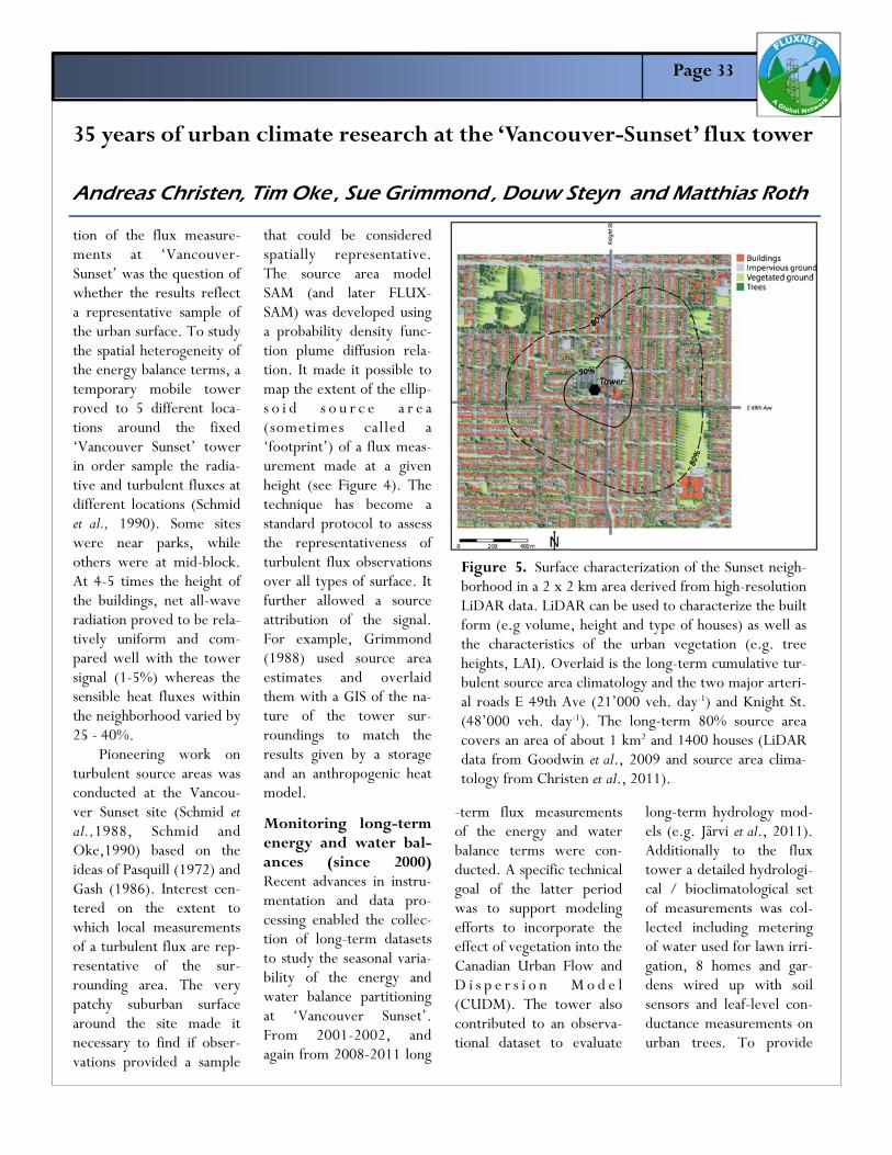
Page 33

tion of the flux measure-ments at ‘Vancouver-Sunset’ was the question of whether the results reflect a representative sample of the urban surface. To study the spatial heterogeneity of the energy balance terms, a temporary mobile tower roved to 5 different loca-tions around the fixed ‘Vancouver Sunset’ tower in order sample the radia-tive and turbulent fluxes at different locations (Schmid et al., 1990). Some sites were near parks, while others were at mid-block. At 4-5 times the height of the buildings, net all-wave radiation proved to be rela-tively uniform and com-pared well with the tower signal (1-5%) whereas the sensible heat fluxes within the neighborhood varied by 25 - 40%. Pioneering work on turbulent source areas was conducted at the Vancou-ver Sunset site (Schmid et al.,1988, Schmid and Oke,1990) based on the ideas of Pasquill (1972) and Gash (1986). Interest cen-tered on the extent to which local measurements of a turbulent flux are rep-resentative of the sur-rounding area. The very patchy suburban surface around the site made it necessary to find if obser-vations provided a sample

that could be considered spatially representative. The source area model SAM (and later FLUX-SAM) was developed using a probability density func-tion plume diffusion rela-tion. It made it possible to map the extent of the ellip-s o i d s o u r c e a r e a (sometimes called a ‘footprint’) of a flux meas-urement made at a given height (see Figure 4). The technique has become a standard protocol to assess the representativeness of turbulent flux observations over all types of surface. It further allowed a source attribution of the signal. For example, Grimmond (1988) used source area estimates and overlaid them with a GIS of the na-ture of the tower sur-roundings to match the results given by a storage and an anthropogenic heat model.

Monitoring long-term energy and water bal-ances (since 2000)Recent advances in instru-mentation and data pro-cessing enabled the collec-tion of long-term datasets to study the seasonal varia-bility of the energy and water balance partitioning at ‘Vancouver Sunset’. From 2001-2002, and again from 2008-2011 long

-term flux measurements of the energy and water balance terms were con-ducted. A specific technical goal of the latter period was to support modeling efforts to incorporate the effect of vegetation into the Canadian Urban Flow and D i s p e r s i o n M o d e l (CUDM). The tower also contributed to an observa-tional dataset to evaluate

long-term hydrology mod-els (e.g. Järvi et al., 2011). Additionally to the flux tower a detailed hydrologi-cal / bioclimatological set of measurements was col-lected including metering of water used for lawn irri-gation, 8 homes and gar-dens wired up with soil sensors and leaf-level con-ductance measurements on urban trees. To provide



Figure 5. Surface characterization of the Sunset neigh-borhood in a 2 x 2 km area derived from high-resolution LiDAR data. LiDAR can be used to characterize the built form (e.g volume, height and type of houses) as well as the characteristics of the urban vegetation (e.g. tree heights, LAI). Overlaid is the long-term cumulative tur-bulent source area climatology and the two major arteri-al roads E 49th Ave (21’000 veh. day-1) and Knight St. (48’000 veh. day-1). The long-term 80% source area covers an area of about 1 km2 and 1400 houses (LiDAR data from Goodwin et al., 2009 and source area clima-tology from Christen et al., 2011).

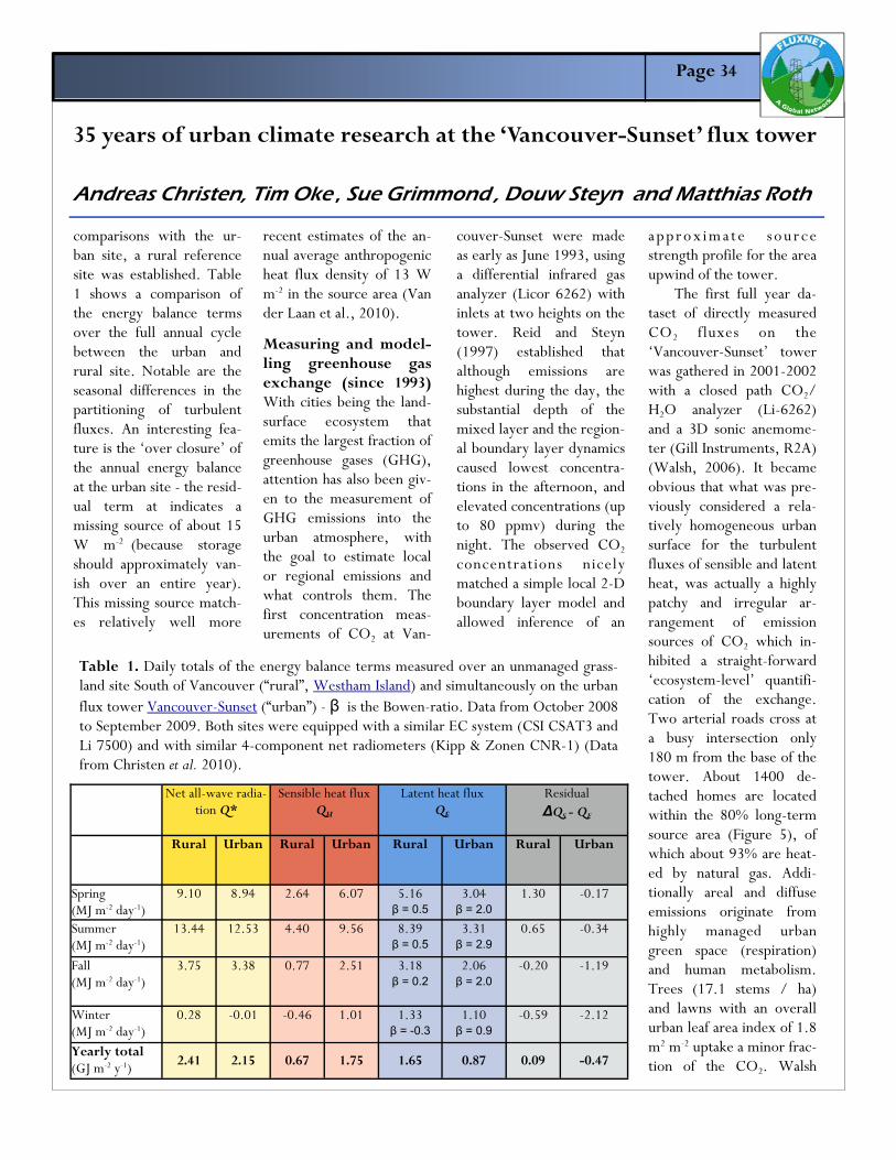
Page 34

comparisons with the ur-ban site, a rural reference site was established. Table 1 shows a comparison of the energy balance terms over the full annual cycle between the urban and rural site. Notable are the seasonal differences in the partitioning of turbulent fluxes. An interesting fea-ture is the ‘over closure’ of the annual energy balance at the urban site - the resid-ual term at indicates a missing source of about 15 W m-2

(because storage should approximately van-ish over an entire year).

This missing source match-es relatively well more

recent estimates of the an-nual average anthropogenic heat flux density of 13 W m-2 in the source area (Van der Laan et al., 2010).

Measuring and model-ling greenhouse gas exchange (since 1993) With cities being the land-surface ecosystem that emits the largest fraction of greenhouse gases (GHG), attention has also been giv-en to the measurement of GHG emissions into the urban atmosphere, with the goal to estimate local or regional emissions and what controls them. The first concentration meas-urements of CO2 at Van-

couver-Sunset were made as early as June 1993, using a differential infrared gas analyzer (Licor 6262) with inlets at two heights on the tower. Reid and Steyn (1997) established that although emissions are highest during the day, the substantial depth of the mixed layer and the region-al boundary layer dynamics caused lowest concentra-tions in the afternoon, and elevated concentrations (up to 80 ppmv) during the night. The observed CO2 concentrations nicely matched a simple local 2-D boundary layer model and allowed inference of an

a p p r o x i m a t e s o u r c e strength profile for the area upwind of the tower. The first full year da-taset of directly measured CO2 fluxes on the ‘Vancouver-Sunset’ tower was gathered in 2001-2002 with a closed path CO2/H2O analyzer (Li-6262) and a 3D sonic anemome-ter (Gill Instruments, R2A) (Walsh, 2006). It became obvious that what was pre-viously considered a rela-tively homogeneous urban surface for the turbulent fluxes of sensible and latent heat, was actually a highly patchy and irregular ar-rangement of emission sources of CO2 which in-hibited a straight-forward ‘ecosystem-level’ quantifi-cation of the exchange. Two arterial roads cross at a busy intersection only 180 m from the base of the tower. About 1400 de-tached homes are located within the 80% long-term source area (Figure 5), of which about 93% are heat-ed by natural gas. Addi-tionally areal and diffuse emissions originate from highly managed urban green space (respiration) and human metabolism. Trees (17.1 stems / ha) and lawns with an overall urban leaf area index of 1.8 m2 m-2 uptake a minor frac-tion of the CO2. Walsh



Net all-wave radia-tion Q*

Sensible heat flux QH

Latent heat flux QE

Residual ∆QS - QF

Rural Urban Rural Urban Rural Urban Rural Urban

Spring (MJ m-2 day-1)

9.10 8.94 2.64 6.07 5.16 β = 0.5

3.04 β = 2.0

1.30 -0.17

Summer (MJ m-2 day-1)

13.44 12.53 4.40 9.56 8.39 β = 0.5

3.31 β = 2.9

0.65 -0.34

Fall (MJ m-2 day-1)

3.75 3.38 0.77 2.51 3.18 β = 0.2

2.06 β = 2.0

-0.20 -1.19

Winter (MJ m-2 day-1)

0.28 -0.01 -0.46 1.01 1.33 β = -0.3

1.10 β = 0.9

-0.59 -2.12

Yearly total (GJ m-2 y-1) 2.41 2.15 0.67 1.75 1.65 0.87 0.09 -0.47

Table 1. Daily totals of the energy balance terms measured over an unmanaged grass-land site South of Vancouver (“rural”, Westham Island) and simultaneously on the urban flux tower Vancouver-Sunset (“urban”) - β is the Bowen-ratio. Data from October 2008 to September 2009. Both sites were equipped with a similar EC system (CSI CSAT3 and Li 7500) and with similar 4-component net radiometers (Kipp & Zonen CNR-1) (Data from Christen et al. 2010).

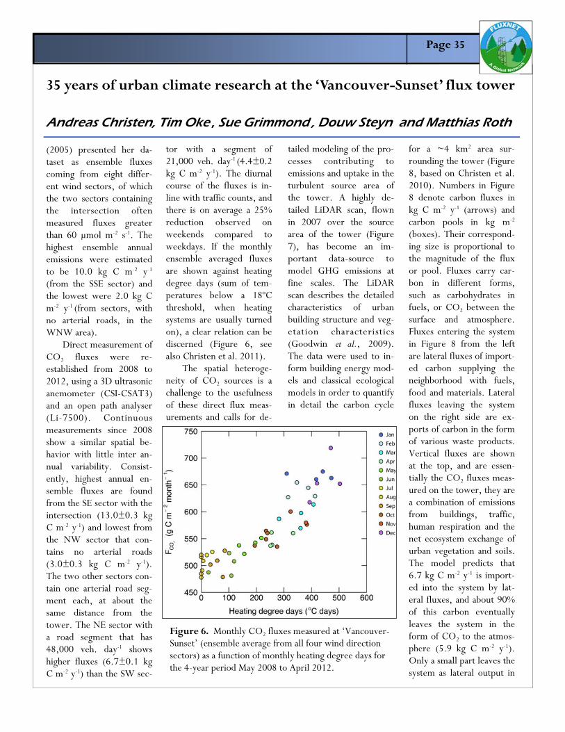
Page 35

(2005) presented her da-taset as ensemble fluxes coming from eight differ-ent wind sectors, of which the two sectors containing the intersection often measured fluxes greater than 60 μmol m-2 s-1. The highest ensemble annual emissions were estimated to be 10.0 kg C m-2 y-1 (from the SSE sector) and the lowest were 2.0 kg C m-2 y-1 (from sectors, with no arterial roads, in the WNW area). Direct measurement of CO2 fluxes were re-established from 2008 to 2012, using a 3D ultrasonic anemometer (CSI-CSAT3) and an open path analyser (Li-7500). Continuous measurements since 2008 show a similar spatial be-havior with little inter an-nual variability. Consist-ently, highest annual en-semble fluxes are found from the SE sector with the intersection (13.0±0.3 kg C m-2 y-1) and lowest from the NW sector that con-tains no arterial roads (3.0±0.3 kg C m-2 y-1). The two other sectors con-tain one arterial road seg-ment each, at about the same distance from the tower. The NE sector with a road segment that has 48,000 veh. day-1 shows higher fluxes (6.7±0.1 kg C m-2 y-1) than the SW sec-

tor with a segment of 21,000 veh. day-1 (4.4±0.2 kg C m-2 y-1). The diurnal course of the fluxes is in-line with traffic counts, and there is on average a 25% reduction observed on weekends compared to weekdays. If the monthly ensemble averaged fluxes are shown against heating degree days (sum of tem-peratures below a 18ºC threshold, when heating systems are usually turned on), a clear relation can be discerned (Figure 6, see also Christen et al. 2011). The spatial heteroge-neity of CO2 sources is a challenge to the usefulness of these direct flux meas-urements and calls for de-

tailed modeling of the pro-cesses contributing to emissions and uptake in the turbulent source area of the tower. A highly de-tailed LiDAR scan, flown in 2007 over the source area of the tower (Figure 7), has become an im-portant data-source to model GHG emissions at fine scales. The LiDAR scan describes the detailed characteristics of urban building structure and veg-etation characteristics (Goodwin et al., 2009). The data were used to in-form building energy mod-els and classical ecological models in order to quantify in detail the carbon cycle

for a ~4 km2 area sur-rounding the tower (Figure 8, based on Christen et al. 2010). Numbers in Figure 8 denote carbon fluxes in kg C m-2 y-1 (arrows) and carbon pools in kg m-2

(boxes). Their correspond-ing size is proportional to the magnitude of the flux or pool. Fluxes carry car-bon in different forms, such as carbohydrates in fuels, or CO2 between the surface and atmosphere. Fluxes entering the system in Figure 8 from the left are lateral fluxes of import-ed carbon supplying the neighborhood with fuels, food and materials. Lateral fluxes leaving the system on the right side are ex-ports of carbon in the form of various waste products. Vertical fluxes are shown at the top, and are essen-tially the CO2 fluxes meas-ured on the tower, they are a combination of emissions from buildings, traffic, human respiration and the net ecosystem exchange of urban vegetation and soils. The model predicts that 6.7 kg C m-2 y-1 is import-ed into the system by lat-eral fluxes, and about 90% of this carbon eventually leaves the system in the form of CO2 to the atmos-phere (5.9 kg C m-2 y-1). Only a small part leaves the system as lateral output in



Figure 6. Monthly CO2 fluxes measured at ‘Vancouver-Sunset’ (ensemble average from all four wind direction sectors) as a function of monthly heating degree days for the 4-year period May 2008 to April 2012.

Page 36

the form of waste (0.8 kg C m-2 y-1). Readers familiar with similar carbon budg-

ets for forests will recog-nize that pathways of car-bon in an urban ecosystem

are linear rather than cyclic and that the 'urban ecosys-tem' is characterized by a

substantial throughput of carbon; most of the im-ported carbon are fossil fuels (>80%). The local storage of carbon is small. Vegetation and soils are moderate pools and most carbon is stored in build-ings – this includes carbon in wooden buildings and furniture. Nevertheless, compared to the fluxes, pools in an urban ecosys-tem are relatively small. This carbon cycle model can be also defined in a spatial context because the location of roads (traffic counts) and build-ings (heating systems) is well known in an urban area. Christen et al. (2011) used a gridded version of this model at a fine resolu-tion of 50m and overlaid turbulent source areas of the EC system on the tow-er. In the annual total the modelled fluxes weighed by the turbulent source area (7.42 kg C m-2 y-1 )

matched reasonably well the measured flux of 6.71 kg C m-2 y-1

determined by means of EC on the tower (given the uncertainty of source area models). This opens up opportunities for flux towers to verify fine-scale pollutant and GHG emission inventories. Most recently, the approach has been extend-



Figure 7. Modeled urban carbon cycle for the Sunset neighborhood. See text for details (modified from Christen et al. 2010).

Page 37

ed to direct EC measure-ments of Methane (CH4)

using a open-path CH4 ana-lyzer (Li7700). Between Feb 2012 and April 2012 an average (net) emission of 17 nmol m-2 s-1 (23.7 mg CH4 m-2 day-1) was record-ed. This flux density matches larger-scale esti-mates for cities and is com-parable to emissions from wetlands. A higher CH4

flux density is measured during the daytime (maximum ~24 nmol m-2 s-1), a lower flux density is recorded in the late night (minimum ~9 nmol m-2 s-

1). Most of the CH4 emit-ted in an urban area can be attributed to incomplete combustion (traffic, space heating / natural gas) and possibly some fugitive emissions of the natural gas network that supplies homes. Uncertain to-date is the contribution of bio-genic processes.

Conclusions

Urban flux towers such as ‘Vancouver-Sunset’ can be a platform to not only quantify the exchange processes over a specific urban area, but more im-portantly are places to de-velop, translate and adapt experimental approaches to complex and extremely rough surfaces. The recent advances in the numerical

modeling of the urban en-vironment (building energy modeling, GHG emission modeling, dispersion and weather forecasting at in-creasingly finer scales) re-quire detailed information on flow, turbulence and land-atmosphere interac-tions in cities. The knowledge and certainty that we can apply theories or use selected parameteri-zations and simplifications originate from experi-mental field research on micrometeorological tow-ers in the urban atmos-phere. Urban measure-ments are also needed to test and verify models. As such, results obtained at ‘Vancouver-Sunset’ are not only of local interest, but have more generally ad-vanced the modeling of weather, climate, hydrolo-gy and emissions in the urban environment. Acknowledgements The unique measurements at Vancouver-Sunset would not have been possible without the continuous financial support of the Natural Science and Engi-neering Research Council of Canada (NSERC) con-tinuously since 1977, and more recently the Canadi-an Foundation for Climate and Atmospheric Sciences

(CFCAS) and the Canadian Foundation for Innova-tion / BCKDF. BC Hydro has provided the University of British Columbia with a long-term permission and commitment that have al-lowed us to operate this unique research facility. References Clarke, J.F., Ching J.K.S., Binkowski F.S., Godowitch J.M., 1978: “Turbulent structure of the urban sur-face boundary layer”, Ninth NATO/CCMS Interna-tional Technical Meeting on Air Pollution Modeling and its Application, Toron-to, ON. Christen, A., Coops N., Kellett R., Crawford B., Heyman E., Olchovski I., Tooke R., van der Laan M., 2010: “A LiDAR-Based Urban Metabolism Approach to Neighbour-hood Scale Energy and Carbon Emissions Model-ling”. University of British Columbia, 2010 Technical report for Natural Re-sources Canada, 104pp.

Christen A., Crawford B., Grimmond S., Voogt J., Oke T. (2010): “Year-long urban-rural differences of the surface radiation and energy balance observed in and near Vancouver, BC”, 44th Annual CMOS Con-

gress / 36th Annual Scientific Meeting of CGU. May 31 - June 4, Ottawa, Canada.

Christen, A., Coops N.C., Crawford B.R., Kellett R., Liss K.N., Olchovski I., Tooke T.R., van der Laan M., Voogt J. A., 2011: “Validation of modeled carbon-dioxide emissions from an urban neighbor-hood with direct eddy-covariance measurements”, Atmospheric Environment, 45, 6057-6069.

Cleugh, H., Oke, T.R. 1986: "Suburban-rural energy balance compari-sons in summer for Van-couver, B.C." Boundary-Layer Meteorology, 36, 351-369.

Gash J.H.C., 1986: “A note on estimating the ef-fect of a limited fetch on micrometeorological evap-oration measurements”, Boundary-Layer Meteorology, 35, 409-413.

Contact

Andreas Christen Department of Geography and Atmospheric Science Program University of British Columbia 132 - 1984 West Mall Vancouver BC V6T 1Z2 Canada [email protected]



Documents

FluxLetter Vol.5 No. 2 March 2013