Embed Size (px)
Citation preview
International Journal of Business and Social Science Vol. 3 No. 10 [Special Issue – May 2012]
145
Forecasting Exchange Rates: a Comparative Analysis
Vincenzo Pacelli
Ph. D. - University of Rome “La Sapienza”
Tenured Assistant Professor of Economics of Financial Intermediaries
University of Foggia
Faculty of Economics
Via Caggese, 1 - 71100 - Foggia - Italy
Abstract
This research aims to analyze and to compare the ability of different mathematical models, such as artificial
neural networks (ANN) and ARCH and GARCH models, to forecast the daily exchange rates Euro/U.S. dollar (USD), identifying which, among all the models applied, produces more accurate forecasts. By empirically
comparing the different mathematical models developed in this research, the traditional indicators for assessing
the relevance of the models show that the ARCH and GARCH models, especially in their static formulations, are
better than the ANN for analyzing and forecasting the dynamics of the exchange rates.
JEL Classification: C3, C5, G14, G20.
Keywords: Exchange Rate; Forecasting; Artificial Neural Networks; ARCH and GARCH models.
1. Introduction
The recent international economic crisis has highlighted the need for banks to implement effective systems for estimating the market risks. In particular, the international activity of the largest banks and the increasing
volatility of exchange rates emphasize the importance of exchange rate risk, whose active management by the
banks require the use of effective forecasting models.
The study of the topic of forecasting in financial markets is based on the research hypotheses that:
(h1 ) the process of pricing in financial markets is not random;
(h2) the degree of information efficiency at Fama of the financial markets is not strong or semi-strong.
If the two research hypotheses proposed were not considered valid, it would be highly redundant and useless to
study the issue of forecasting in financial markets.
This research aims to analyze and to compare the ability of different mathematical models, such as artificial
neural networks (ANN) and ARCH and GARCH models, to highlight non-random and therefore predictable
behaviour in a highly liquid market and therefore characterized by high efficiency, such as the exchange rate Euro/US dollar. So a non-linear model of ANN and different ARCH and GARCH models were developed and
empirically tested to forecast the daily exchange rates Euro/U.S. dollar (USD), identifying which, among all the
models applied, produces more accurate forecasts. After developing and applying empirically the ANN and alternative formulations of the ARCH and GARCH models with different number of parameters (lags p and
q), this research compares these formulations using the traditional indicators for assessing the relevance of the
models, leading to interesting conclusions about which is the model characterized by better forecasting ability.
2. A Literature Review
The economic theory has not yet provided econometric models to produce efficient forecasts of exchange rates,
although many studies have been devoted to the estimation of the equilibrium of exchange rates from the 20s to the recent years [Cassel (1923); Samuelson (1964); Mundell (1968); Dornbusch (1973 and 1979); Allen and
Kenen (1980); Frankel and Mussa (1985); MacDonald (1999); Rogoff (1999); Alba e Papell (2007); Kim B.H.,
Kim H.K. and Oh (2009); Taylor (2009); Grossmann, Simpson e Brown (2009)]. In particular, Meese and Rogoff
(1983) found that none of the forecasting models of the exchange rate established by economic theory has a better ability to forecast, over a period lower than 12 months, rather than the forward rate models or random walk,
emphasizing the paradox that the variations of exchange rates are completely random.
The Special Issue on Social Science Research © Centre for Promoting Ideas, USA www.ijbssnet.com
146
In the wake of the study of Meese and Rogoff, some authors, including Hsieh (1989), Refenes, Azema-Barac,
Chen, Karoussous (1993), Nabney, Dunis, Dallaway, Leong, Redshaw (1996), Brooks (1996 and 1997), Tenti (1996), Lawrence, Giles, Tsoi (1997), Gabbi (1999), Gencay (1999), Soofi, Cao (1999), Alvarez and Alvarez-
Diaz (2003, 2005 and 2007) Alvarez-Diaz (2008), Reitz and Taylor (2008), Anastakis and Mort (2009), Majhi,
Panda and Sahoo (2009), Bereau, Lopez and Villavicencio (2010), Bildirici, Alp and Ersen (2010), have studied
the predictability of the dynamics of exchange rates of non-linear models such as artificial neural networks, genetic algorithms, expert systems or fuzzy models, leading however to conflicting results.
Mandelbrot (1963) and Fama (1965) have shown that the time series of exchange rates are generally characterized by conditional heteroskedasticity, leptocurtosis and volatility clustering. These features of the series of the
exchange rates therefore imply the rejection of the hypothesis of normality, as these financial series show
alternating periods characterized by large fluctuations around the average value with periods characterized by
smaller variations. In this framework, numerous studies on econometric models were carried out, such as on ARCH and GARCH models, which are able to analyze and perceive the time variability of the phenomenon
of volatility, and are therefore useful tools to capture the non-linearity of the changes in exchange rates (Krager
and Kugler, 1993; Rossi, 1995; Brooks, 1996 and 1997; Bali and Guirguis, 2007; Wang, Chen, Jin and Zhou, 2010).
The pioneers of the ARCH (Autoregressive Conditional Heteroschedasticity) models were Engle (1982) and Bollerslev (1986), who generalized the model of Engle opening the way for a new generation of models able to
capture the dynamics of time series, the GARCH (Generalized Autoregressive Conditional Heteroschedasticity)
models. Over the years other contributions have extended the GARCH models in to two directions: univariate and multivariate models. The first category includes the E-GARCH model (Exponential GARCH) of Nelson (1991),
the T-GARCH model (Threshold GARCH) of Glosten, Jagannathan and Runkle (1993), the Q-GARCH model
(Quadratic GARCH) of Sentana (1995). The second category includes the VECH model of Bollerslev, Engle and
Wooldridge (1988), the BEKK model formalized by Engle and Kroner (1995), the O-GARCH model (Orthogonal GARCH) of Alexander and Chibumba (1996) and the GO-GARCH (Generalized Orthogonal GARCH) of Van
der Weide (2002).
3. The Methodology
The prediction of the financial time series, as the exchange rates, requires the prior identification of a specific
portfolio of variables (input data for forecasting models) which are explanatory of the phenomenon to be foreseen and therefore significantly influence the pricing (output for forecasting models). The forecasting models, in fact,
will learn the characteristics of the phenomenon to be foreseen by the variables of input selected and by the
historical data that represent the phenomenon analyzed. The models predicting exchange rates, developed by the
economic theory over the years, can be classified into two main categories:
structural prediction models or linear ones, such as econometric models as Autoregressive Conditional
Heteroschedasticity (ARCH), Generalized Autoregressive Conditional Heteroschedasticity (GARCH), State
Space, which are based on the general view that every action of traders can be explained by a model of
behaviour and thus by a definite, explicit function that can bind variables determinants of the phenomenon to be foreseen;
black box forecasting models or non-linear ones, such as artificial neural networks, genetic algorithms,
expert systems or fuzzy models, which, through the learning of the problem analyzed, attempt to identify and predict the non random and non-linear dynamics of prices, but without explicit ties and logical functions that
bind the variables analyzed.
This paper aims to analyze and to compare the ability of different mathematical models belonging from the two
categories, such as artificial neural networks (ANN) and ARCH and GARCH models, to forecast the exchange
rate Eur/ Usd.
3.1. The Methodology for the Development of the Artificial Neural Network Model (ANNm)
The objective of the ANN developed is to predict the trend of the exchange rate Euro / USD up to three days
ahead of last data available. The variable of output of the ANN designed is then the daily exchange rate
Euro/Dollar and the frequency of data collection of variables of input and the output is daily.

International Journal of Business and Social Science Vol. 3 No. 10 [Special Issue – May 2012]
147
The construction of the data base used to train the artificial neural network (ANN) developed was divided into the
following three phases:
data collection;
data analysis;
variable selection.
The phase of data collection must achieve the following objectives:
regularity in the frequency of the data collection by the markets;
homogeneity between the information provided to the ANN and that available for the market operators.
In the phase of the data collection, both macro-economic variables (fundamental data) and market data were,
therefore, initially considered as variables of input, from which it was assumed that the behaviour of the exchange
rate euro-dollar was conditional. The data were collected from the 1st January, 1999 to December 31, 2009
1.
Once collected all the data, there was the stage of their analysis, which aims to select the data, that will be used to
train ANN, among those initially collected. This phase is crucial, because the learning capacity of the ANN
depends on the quality of information provided, which is the capacity of this information to provide a true representation of the phenomenon without producing ambiguous, distorting or amplifying effects in the phases of
training networks.
In this phase, the observation of the correlation or similarity coefficients allow to evaluate the nature of relations
between the variables of input considered, suggesting the elimination of the variables highly correlated with each
other and therefore capable to product amplifying or distorting effects during the training phases (Pacelli,
Bevilacqua, Azzollini, 2011).
Following the analysis of the correlation coefficients, there was the stage of selection of variables and the
variables with the following characteristics were eliminated:
variables characterized by a Pearson correlation coefficient with at least one other variable considered above
the threshold level of acceptance equal to 0,80;
monthly variables, because, having developed a neural network with a daily frequency of data collection of variables of input and output, they were considered potentially able to produce ambiguous or redundant
signals during the training of ANN.
As a result of the selection of variables conducted according to the criteria outlined above, the following seven
variables of input of the ANN were selected:
Nasdaq Index;
Daily Exchange Rate Eur/Usd New Zeland;
Gold Spot Price Usa; Average returns of Government Bonds - 5 years in the Usa zone;
Average returns of Government Bonds - 5 years in the Eurozone;
Crude Oil Price – CLA (Crude oil); Exchange rate Euro / US dollar of the previous day compared to the day of the output.
In establishing the final data set with data of the seven input variables, exceptional values, as the outliers, were
also removed related to special historical events such as the terrorist attacks of September 11, 2001.
For each of these variables of input, historical memory was calculated, which is the number of daily observations in which it is very high the possibility that the daily value of the variables is self-correlated with the values of n
days2.
The historical memory was calculated by a polynomial interpolation with coefficient R2 equal to 0,98 for 90% of
cases. The historical memories calculated for each variable are:
Nasdaq index: eight surveys;
Daily exchange rate Euro / NZ Dollar: five surveys;
1 Source of data are Bloomberg and Borsa Italiana. 2 The construction of the data set of the ANN is based on the concept of historical memory as the objective of the ANN is to
predict the trend of the exchange rate Euro / Dollar.
The Special Issue on Social Science Research © Centre for Promoting Ideas, USA www.ijbssnet.com
148
Spot price of gold expressed in dollars per ounce: six surveys;
Average returns of government bonds - 5 years in the USA: eight surveys; Average returns of government bonds - 5 years in the Eurozone: seven surveys;
The price of crude oil (CLA): eight surveys;
Exchange rate Euro / USD: seven surveys more output3;
In order to predict the trend of historical memories of individual variables by determining the angular coefficients
(m), it was used by the software MatLab the function Polyfit, whereas for the first experiments a degree of the
polynomial approximation of 1.
Since the ANN uses values between -1 and 1 where it is used the activation function Tansig4, it was necessary to
normalize data through the interpolation performed with MatLab, assigning values between -1 and 1 to vary of the
value of the angular coefficient (m) produced by the Polyfit, according to the following summary:
IF 0<=m<=0.1 Then value =0.2 IF 0.1<m<=1.1 Then value =0.4
IF 1.1<m<=3.1 Then value =0.6
IF 3.1<m<=7.1 Then value =0.8 IF m>7.1 Then value =1
IF -0.1<=m<0 Then value =-0.2
IF -1.1<=m<-0.1 Then value =-0.4 IF -3.1<=m<-0.1 Then value =-0.6
IF -7.1<=m<3.1 Then value =-0.8
IF m<-7.1 Then value =-1
As shown by the previous scheme, the change of the angular coefficient determines the change in trend growth or
reduction of the exchange rate Euro / USD.
The inputs of the network were reduced by 49 (i.e. 7 input with their historical memories) to 7, while the records
are 547.
An innovative genetic algorithm multi-objective was used to solve the problem of finding the optimal topology of
a Multi Layer Perceptron (MLP) neural network as a trade-off between the performance in terms of precision and
the performance in terms of generalization, avoiding the problems of overfitting during the training phase (Pacelli, Bevilacqua, Azzollini, 2011). In this paper each MLP neural topology developed for this research was
trained on data sets described in this paragraph by monitoring two parameters of precision and generalization.
Generalization and accuracy were calculated as mean square error over all 120 training examples and all 40 examples of validation considered. In particular, for the purposes of this research, the optimal MLP neural
network topology has been designed and tested by means the specific genetic algorithm multi-objective Pareto-
Based designed from Bevilacqua et al. (2006).
3.2. The Methodology: the ARCH and GARCH Models
The ARCH (Auto Regressive Conditionally Heteroskedasticity) model, introduced by Engle in 1982, is one of the
main methods used to analyze financial time series.
In a simplified version of the model proposed by Engle, the ARCH process is expressed by the following relation:
Yt = ϕjxt,j + et
k
j=1
3 To train the ANN, it is considered as current moment t-2 for each variable, as to obtain two readings back in order to predict
a trend output rate Eur / U.S. dollar equal to three days. 4 Hyperbolic tangent sigmoid activation function: Tansig (n) = 2 / (1 + exp (-2 * n)) -1, where n is the matrix of inputs. The
results of a function Tansig can vary between -1 and 1.
(a)
International Journal of Business and Social Science Vol. 3 No. 10 [Special Issue – May 2012]
149
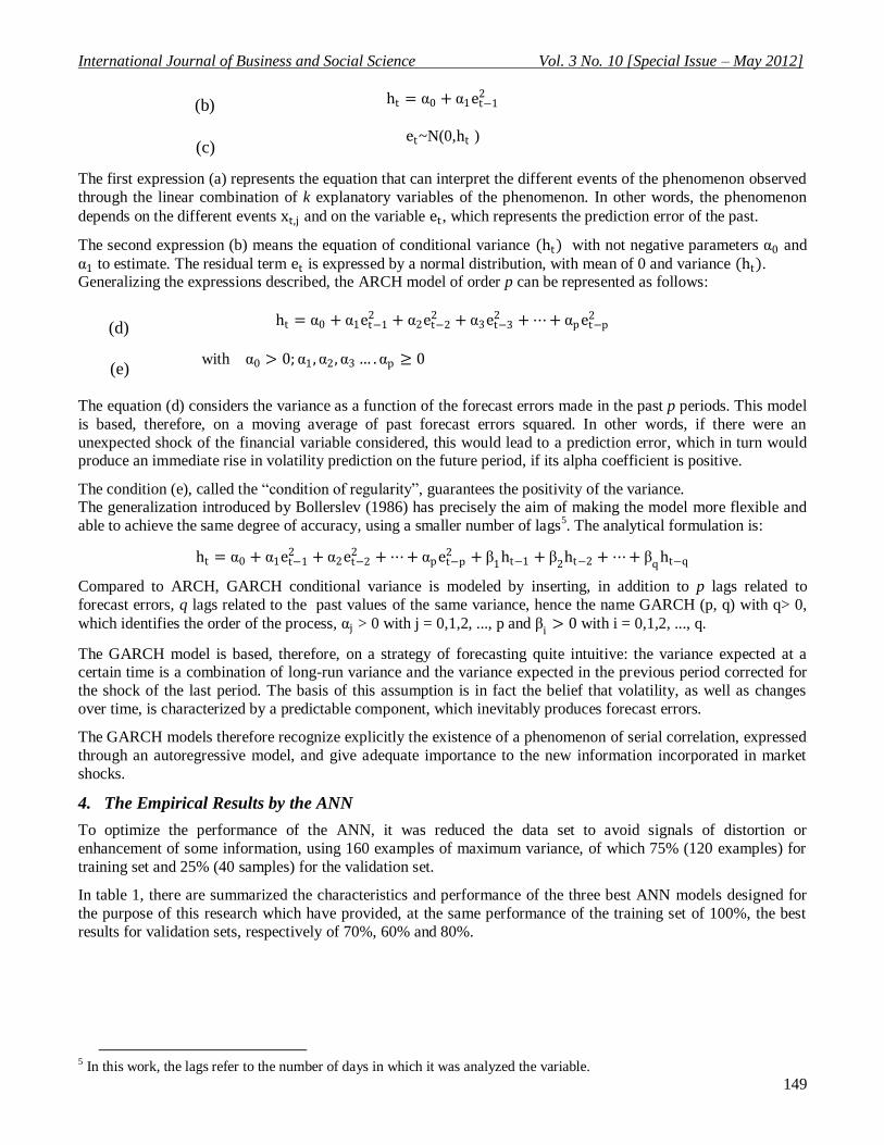
ht = α0 + α1et−12
et~N(0,ht )
The first expression (a) represents the equation that can interpret the different events of the phenomenon observed
through the linear combination of k explanatory variables of the phenomenon. In other words, the phenomenon
depends on the different events xt,j and on the variable et , which represents the prediction error of the past.
The second expression (b) means the equation of conditional variance (ht) with not negative parameters α0 and
α1 to estimate. The residual term et is expressed by a normal distribution, with mean of 0 and variance (ht). Generalizing the expressions described, the ARCH model of order p can be represented as follows:
ht = α0 + α1et−12 + α2et−2
2 + α3et−32 + ⋯ + αp et−p
2
with α0 > 0; α1, α2 , α3 … . αp ≥ 0
The equation (d) considers the variance as a function of the forecast errors made in the past p periods. This model
is based, therefore, on a moving average of past forecast errors squared. In other words, if there were an
unexpected shock of the financial variable considered, this would lead to a prediction error, which in turn would produce an immediate rise in volatility prediction on the future period, if its alpha coefficient is positive.
The condition (e), called the “condition of regularity”, guarantees the positivity of the variance. The generalization introduced by Bollerslev (1986) has precisely the aim of making the model more flexible and
able to achieve the same degree of accuracy, using a smaller number of lags5. The analytical formulation is:
ht = α0 + α1et−12 + α2et−2
2 + ⋯ + αp et−p2 + β
1ht−1 + β
2ht−2 + ⋯ + β
qht−q
Compared to ARCH, GARCH conditional variance is modeled by inserting, in addition to p lags related to
forecast errors, q lags related to the past values of the same variance, hence the name GARCH (p, q) with q> 0,
which identifies the order of the process, αj > 0 with j = 0,1,2, ..., p and βi
> 0 with i = 0,1,2, ..., q.
The GARCH model is based, therefore, on a strategy of forecasting quite intuitive: the variance expected at a certain time is a combination of long-run variance and the variance expected in the previous period corrected for
the shock of the last period. The basis of this assumption is in fact the belief that volatility, as well as changes
over time, is characterized by a predictable component, which inevitably produces forecast errors.
The GARCH models therefore recognize explicitly the existence of a phenomenon of serial correlation, expressed
through an autoregressive model, and give adequate importance to the new information incorporated in market
shocks.
4. The Empirical Results by the ANN
To optimize the performance of the ANN, it was reduced the data set to avoid signals of distortion or
enhancement of some information, using 160 examples of maximum variance, of which 75% (120 examples) for
training set and 25% (40 samples) for the validation set.
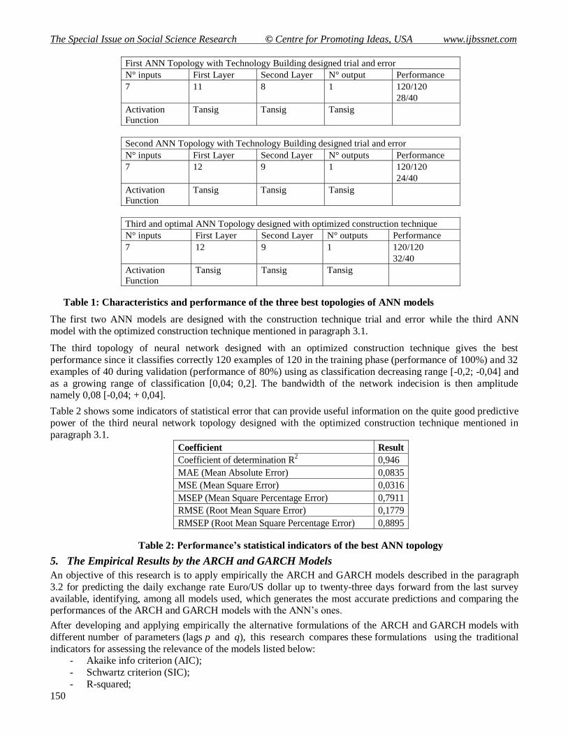
In table 1, there are summarized the characteristics and performance of the three best ANN models designed for
the purpose of this research which have provided, at the same performance of the training set of 100%, the best
results for validation sets, respectively of 70%, 60% and 80%.
5 In this work, the lags refer to the number of days in which it was analyzed the variable.
(b)
(c)
(d)
(e)
The Special Issue on Social Science Research © Centre for Promoting Ideas, USA www.ijbssnet.com
150
Table 1: Characteristics and performance of the three best topologies of ANN models
The first two ANN models are designed with the construction technique trial and error while the third ANN
model with the optimized construction technique mentioned in paragraph 3.1.
The third topology of neural network designed with an optimized construction technique gives the best
performance since it classifies correctly 120 examples of 120 in the training phase (performance of 100%) and 32
examples of 40 during validation (performance of 80%) using as classification decreasing range [-0,2; -0,04] and
as a growing range of classification [0,04; 0,2]. The bandwidth of the network indecision is then amplitude namely 0,08 [-0,04; + 0,04].
Table 2 shows some indicators of statistical error that can provide useful information on the quite good predictive
power of the third neural network topology designed with the optimized construction technique mentioned in
paragraph 3.1.
Table 2: Performance’s statistical indicators of the best ANN topology
5. The Empirical Results by the ARCH and GARCH Models
An objective of this research is to apply empirically the ARCH and GARCH models described in the paragraph
3.2 for predicting the daily exchange rate Euro/US dollar up to twenty-three days forward from the last survey
available, identifying, among all models used, which generates the most accurate predictions and comparing the performances of the ARCH and GARCH models with the ANN’s ones.
After developing and applying empirically the alternative formulations of the ARCH and GARCH models with
different number of parameters (lags p and q), this research compares these formulations using the traditional
indicators for assessing the relevance of the models listed below: - Akaike info criterion (AIC);
- Schwartz criterion (SIC);
- R-squared;
First ANN Topology with Technology Building designed trial and error
N° inputs First Layer Second Layer N° output Performance
7 11 8 1 120/120
28/40
Activation
Function
Tansig Tansig Tansig
Second ANN Topology with Technology Building designed trial and error
N° inputs First Layer Second Layer N° outputs Performance
7 12 9 1 120/120
24/40
Activation
Function
Tansig Tansig Tansig
Third and optimal ANN Topology designed with optimized construction technique
N° inputs First Layer Second Layer N° outputs Performance
7 12 9 1 120/120
32/40
Activation
Function
Tansig Tansig Tansig
Coefficient Result
Coefficient of determination R2 0,946
MAE (Mean Absolute Error) 0,0835
MSE (Mean Square Error) 0,0316
MSEP (Mean Square Percentage Error) 0,7911
RMSE (Root Mean Square Error) 0,1779
RMSEP (Root Mean Square Percentage Error) 0,8895
International Journal of Business and Social Science Vol. 3 No. 10 [Special Issue – May 2012]
151
- Adjusted R-squared;
- Standard deviation.
The empirical analysis was conducted on a series of daily data of the exchange rate Euro/U.S. dollar related to the
period from December 31, 2008 until December 31, 2009.
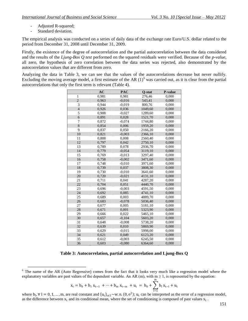
Firstly, the existence of the degree of autocorrelation and the partial autocorrelation between the data considered
and the results of the Ljung-Box Q test performed on the squared residuals were verified. Because of the p-value,
all zero, the hypothesis of zero correlation between the data series was rejected, also demonstrated by the autocorrelation values that are different from zero.
Analyzing the data in Table 3, we can see that the values of the autocorrelations decrease but never nullify.
Excluding the moving average model, a first estimate of the AR (1)6 was carried out, as it is clear from the partial
autocorrelations that only the first term is relevant (Table 4).
AC PAC Q-stat P-value
1 0,981 0,981 276,46 0,000 2 0,963 -0,016 543,41 0,000
3 0,944 -0,019 800,76 0,000 4 0,926 0,036 1049,60 0,000 5 0,908 -0,027 1289,60 0,000 6 0,891 0,028 1521,70 0,000 7 0,872 -0,074 1744,80 0,000
8 0,854 0,006 1959,20 0,000 9 0,837 0,050 2166,20 0,000 10 0,821 -0,003 2366,10 0,000 11 0,808 0,008 2560,40 0,000 12 0,797 0,042 2750,10 0,000 13 0,789 0,078 2936,70 0,000 14 0,779 -0,054 3119,10 0,000 15 0,769 -0,013 3297,40 0,000
16 0,758 -0,002 3471,60 0,000 17 0,748 -0,010 3971,60 0,000 18 0,739 0,037 3808,30 0,000 19 0,730 -0,010 3641,60 0,000 20 0,720 -0,021 4131,10 0,000 21 0,711 0,041 4287,20 0,000 22 0,704 0,051 4440,70 0,000 23 0,696 -0,003 4591,50 0,000 24 0,692 0,085 4741,10 0,000
25 0,689 0,003 4889,70 0,000 26 0,683 -0,078 5036,40 0,000 27 0,677 0,005 5181,10 0,000 28 0,671 0,001 5323,90 0,000 29 0,666 0,022 5465,10 0,000 30 0,657 -0,104 5603,20 0,000 31 0,648 -0,008 5738,20 0,000 32 0,639 0,010 5869,90 0,000
33 0,629 -0,015 5998,00 0,000 34 0,621 0,049 6123,20 0,000 35 0,612 -0,003 6245,50 0,000 36 0,603 -0,080 6364,60 0,000
Table 3: Autocorrelation, partial autocorrelation and Ljung-Box Q
6 The name of the AR (Auto Regressive) comes from the fact that it looks very much like a regression model where the
explanatory variables are past values of the dependent variable. An AR (m), with m ≥ 1, is represented by the equation:
xt = b0 + b1 xt−1 + ⋯ + bm xt−m + ut = b0 + bl xt−l
m
l=1
+ ut
where bl , ∀ l = 0, 1, … , m, are real constant and ut t∈T~w. n. 0, σ2 ; ut can be interpreted as the error of a regression model,
as the difference between xt and its conditional mean, where the set of conditioning is composed of past values xt .
The Special Issue on Social Science Research © Centre for Promoting Ideas, USA www.ijbssnet.com
152
Variable Coefficient
Standard
Error
T
Statistics P-value
C 1,4528 0,0713 20,3845 0,0000
AR(1) 0,9864 0,0099 99,5965 0,0000
F Statistics 9919,4560
P-value 0,0000
log-likelihood 795,6307
Akaike info criterion (AIC) -6,1049
Schwarz criterion (SIC) -6,0775
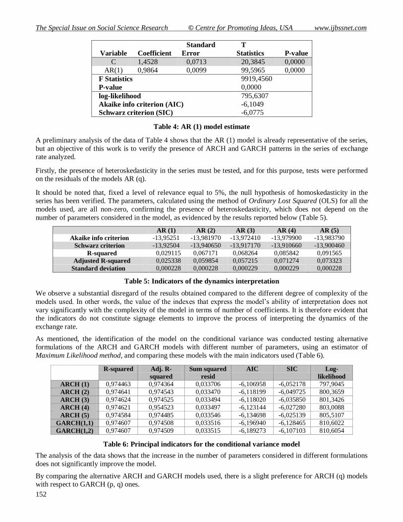
Table 4: AR (1) model estimate
A preliminary analysis of the data of Table 4 shows that the AR (1) model is already representative of the series,
but an objective of this work is to verify the presence of ARCH and GARCH patterns in the series of exchange rate analyzed.
Firstly, the presence of heteroskedasticity in the series must be tested, and for this purpose, tests were performed on the residuals of the models AR (q).
It should be noted that, fixed a level of relevance equal to 5%, the null hypothesis of homoskedasticity in the series has been verified. The parameters, calculated using the method of Ordinary Lost Squared (OLS) for all the
models used, are all non-zero, confirming the presence of heteroskedasticity, which does not depend on the
number of parameters considered in the model, as evidenced by the results reported below (Table 5).
AR (1) AR (2) AR (3) AR (4) AR (5)
Akaike info criterion -13,95251 -13,981970 -13,972410 -13,979900 -13,983790
Schwarz criterion -13,92504 -13,940650 -13,917170 -13,910660 -13,900460
R-squared 0,029115 0,067171 0,068264 0,085842 0,091565
Adjusted R-squared 0,025338 0,059854 0,057215 0,071274 0,073323
Standard deviation 0,000228 0,000228 0,000229 0,000229 0,000228
Table 5: Indicators of the dynamics interpretation
We observe a substantial disregard of the results obtained compared to the different degree of complexity of the
models used. In other words, the value of the indexes that express the model’s ability of interpretation does not
vary significantly with the complexity of the model in terms of number of coefficients. It is therefore evident that the indicators do not constitute signage elements to improve the process of interpreting the dynamics of the
exchange rate.
As mentioned, the identification of the model on the conditional variance was conducted testing alternative formulations of the ARCH and GARCH models with different number of parameters, using an estimator of
Maximum Likelihood method, and comparing these models with the main indicators used (Table 6).
R-squared Adj. R-
squared
Sum squared
resid
AIC SIC Log-
likelihood
ARCH (1) 0,974463 0,974364 0,033706 -6,106958 -6,052178 797,9045
ARCH (2) 0,974641 0,974543 0,033470 -6,118199 -6,049725 800,3659
ARCH (3) 0,974624 0,974525 0,033494 -6,118020 -6,035850 801,3426
ARCH (4) 0,974621 0,954523 0,033497 -6,123144 -6,027280 803,0088
ARCH (5) 0,974584 0,974485 0,033546 -6,134698 -6,025139 805,5107
GARCH(1,1) 0,974607 0,974508 0,033516 -6,196940 -6,128465 810,6022
GARCH(1,2) 0,974607 0,974509 0,033515 -6,189273 -6,107103 810,6054
Table 6: Principal indicators for the conditional variance model
The analysis of the data shows that the increase in the number of parameters considered in different formulations
does not significantly improve the model.
By comparing the alternative ARCH and GARCH models used, there is a slight preference for ARCH (q) models with respect to GARCH (p, q) ones.
International Journal of Business and Social Science Vol. 3 No. 10 [Special Issue – May 2012]
153
The models described above can then be used for interesting operating applications in finance, as forecasting
financial series of data or trading.
Assuming that at the basis of all forecasts there is the volatility, as the uncertainty observed in the markets, and
that it is identified with the conditional variance on previous information and available at a given instant of time, in this research ARCH and GARCH models, constructed and described previously, are used to predict the
exchange rate Euro/US Dollar.
Using a sample consisting of N observations and fixed H <N, the aim is to make predictions for the times H +1, H +2, ..., N.
We represent two prediction models:
- the static forecast (Table 7): the prediction uses only the number of observed data, increased by a factor at
every step: in this case fH+1with the series x1, x2 , … , xH, fH+2 with x1, x2, … , xH, xH+1 ,.. and fN with
x1, x2, … , xH , xH+1,… , xN-1 are calculated;
- the dynamic forecast (Table 8): expected values are calculated using the series of observed data at the
period before the prediction: after the first period, the observed data are replaced by the corresponding
amounts previously provided for, as fH+1 is calculated using the series 𝑥1 , 𝑥2, … , 𝑥H, the value of fH+2 is
calculated with the series 𝑥1, 𝑥2, … , 𝑥H, fH+1, and so on until it is estimated fN with the series
𝑥1, 𝑥2, … , 𝑥H, fH+1, … , fN-1.
All predictions were made with twenty-three days after the last survey. In order to test the forecasting ability of the models used, in addition to the theoretical values obtained by the empirical application of the models, we have
calculated the actual historical values, that represent the terms of comparison in the process of performance
evaluation of the forecasting models used.
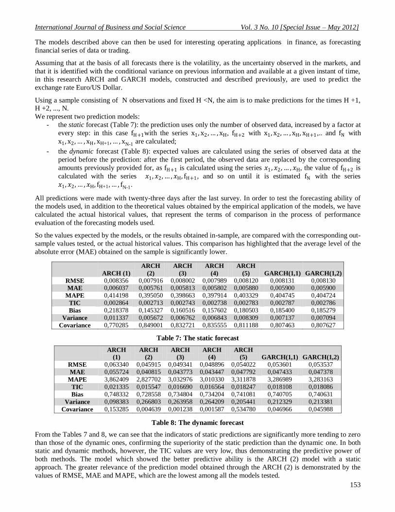
So the values expected by the models, or the results obtained in-sample, are compared with the corresponding out-
sample values tested, or the actual historical values. This comparison has highlighted that the average level of the
absolute error (MAE) obtained on the sample is significantly lower.
ARCH (1)
ARCH
(2)
ARCH
(3)
ARCH
(4)
ARCH
(5) GARCH(1,1) GARCH(1,2)
RMSE 0,008356 0,007916 0,008002 0,007989 0,008120 0,008131 0,008130
MAE 0,006037 0,005761 0,005813 0,005802 0,005880 0,005900 0,005900
MAPE 0,414198 0,395050 0,398663 0,397914 0,403329 0,404745 0,404724
TIC 0,002864 0,002713 0,002743 0,002738 0,002783 0,002787 0,002786
Bias 0,218378 0,145327 0,160516 0,157602 0,180503 0,185400 0,185279
Variance 0,011337 0,005672 0,006762 0,006843 0,008309 0,007137 0,007094
Covariance 0,770285 0,849001 0,832721 0,835555 0,811188 0,807463 0,807627
Table 7: The static forecast
ARCH
(1)
ARCH
(2)
ARCH
(3)
ARCH
(4)
ARCH
(5) GARCH(1,1) GARCH(1,2)
RMSE 0,063340 0,045915 0,049341 0,048896 0,054022 0,053601 0,053537
MAE 0,055724 0,040815 0,043773 0,043447 0,047792 0,047433 0,047378
MAPE 3,862409 2,827702 3,032976 3,010330 3,311878 3,286989 3,283163
TIC 0,021335 0,015547 0,016690 0,016564 0,018247 0,018108 0,018086
Bias 0,748332 0,728558 0,734804 0,734204 0,741081 0,740705 0,740631
Variance 0,098383 0,266803 0,263958 0,264209 0,205441 0,212329 0,213381
Covariance 0,153285 0,004639 0,001238 0,001587 0,534780 0,046966 0,045988
Table 8: The dynamic forecast
From the Tables 7 and 8, we can see that the indicators of static predictions are significantly more tending to zero
than those of the dynamic ones, confirming the superiority of the static prediction than the dynamic one. In both static and dynamic methods, however, the TIC values are very low, thus demonstrating the predictive power of
both methods. The model which showed the better predictive ability is the ARCH (2) model with a static
approach. The greater relevance of the prediction model obtained through the ARCH (2) is demonstrated by the
values of RMSE, MAE and MAPE, which are the lowest among all the models tested.
The Special Issue on Social Science Research © Centre for Promoting Ideas, USA www.ijbssnet.com
154
6. Concluding Remarks
By the analysis of the empirical results, it is possible to say, first of all, that the empirical research conducted
largely support the two research hypothesis discussed in section 1, justifying the attempt to forecast the exchange
rate Euro / USD performed in this research. The good forecasting performances of the different models developed show that the process of formation of the exchange rates is not completely governed by noise.
Furthermore by comparing the ability of the different mathematical models developed in this research, such as an
artificial neural network (ANN) and different ARCH and GARCH models, the traditional indicators for assessing the relevance of the models show that the ARCH and GARCH models, especially in their static formulations, are
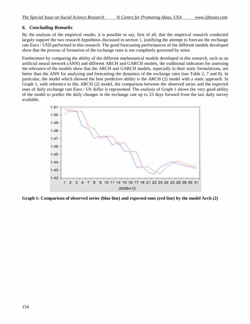
better than the ANN for analyzing and forecasting the dynamics of the exchange rates (see Table 2, 7 and 8). In
particular, the model which showed the best predictive ability is the ARCH (2) model with a static approach. In Graph 1, with reference to this ARCH (2) model, the comparison between the observed series and the expected
ones of daily exchange rate Euro / US dollar is represented. The analysis of Graph 1 shows the very good ability
of the model to predict the daily changes in the exchange rate up to 23 days forward from the last daily survey available.
Graph 1: Comparison of observed series (blue line) and expected ones (red line) by the model Arch (2)
International Journal of Business and Social Science Vol. 3 No. 10 [Special Issue – May 2012]
155
References
Alba J. D., Papell D. H. (2007), “Purchasing power parity and country characteristics: Evidence from panel data tests”,
in Journal of Development Economics, Volume 83, Issue 1, May , pp. 240-251.
Alexander C., Chibumba A. (1996), “Multivariate orthogonal factor GARCH”, in Discussion Paper in mathematics,
University of Sussex.
Allen P. R., Kenen P. B. (1980), Asset Markets, Exchange Rates, and Economic Integration, Cambridge University
Press, London.
Alvarez-Dıaz M., Alvarez A. (2003), “Forecasting exchange rates using genetic algorithms”, in Applied Economics Letters, Volume 10, pp. 319–22.
Alvarez-Dıaz M., Alvarez A. (2005), “Genetic multimodel composite forecast for non-linear forecasting of exchange
rates”, in Empirical Economics, Volume 30, pp. 643–63.
Alvarez-Dıaz M., Alvarez A. (2007), “Forecasting exchange rates using an evolutionary neural network”, in Applied
Financial Economics Letters, Volume 3, pp.5–9.
Alvarez-Diaz M. (2008), “Exchange rates forecasting: local or global method?”, in Applied Financial Economics Letters, Volume 40, pp. 1969-1984.
Anastakis L., Mort N. (2009), ”Exchange rate forecasting using a combined parametric and nonparametric self-
organising modelling approach”, in Expert Systems with Applications, Volume 36, Issue 10, December, pp.
12001-12011.
Bali R., Guirguis H. (2007), “Extreme observations and non-normality in ARCH and GARCH”, in International Review of Economics & Finance, n. 16, Issue 3, pp. 332-346.
Bereau S., Lopez Villavicencio A., Mignon V. (2010), “Nonlinear adjustment of the real exchange rate towards its
equilibrium value: A panel smooth transition error correction modelling”, in Economic Modelling, Volume 27,
Issue 1, January, pp. 404-416.
Bevilacqua V., Mastronardi G., Menolascina F., Pannarale P., Pedone A. (2006), “A Novel Multi-Objective Genetic
Algorithm Approach to Artificial Neural Network Topology Optimisation: The Breast Cancer Classification
Problem”, in Proceedings of 2006 International Joint Conference on Neural Networks IEEE 06CH37726D,
pp. 7803-9489-5.
Bildirici M., Alp E. A., Ersin O. (2010), “TAR-cointegration neural network model: An empirical analysis of exchange
rates and stock returns”, in Expert Systems with Applications, Volume 37, Issue 1, January pp. 2-11.
Bollerslev T. (1986), “Generalized autoregressive conditional heteroskedasticity”, in Journal of Econometrics, n. 31,
pp. 307–327.
Bollerslev T., Engle R. F., Wooldridge J. M. (1988), “A capital asset pricing model with time varying covariances”, in
Journal of Political Economy, n. 96, pp. 116–131.
Brooks C. (1996), “Testing for Nonlinearity in Daily Pound Exchange Rates”, in Applied Financial Economics, Volume 6, pp. 307-317.
Brooks C. (1997), “Linear and non-linear (non-) forecastability of highfrequency exchange rates”, in Journal of
forecasting, n. 16, pp. 125-145.
Cassel G. (1923), Money and Foreign Exchange, Macmillan, New York
Dornbusch R. (1973), “Currency Depreciation, Hoarding and relative Prices”, in Journal of political Economy, pp. 893-
915.
Dornbusch R. (1979), “Monetary policy under Exchange Rate Flexibility”, in Managed Exchange Rate Flexibility: The Recent Experience, Federal Reserve Bank of Boston, Conference Series Volume 20, pp. 90-122.
Dornbusch R. (1987), Purchaising Power of Money, in The New Palgrave, Stockton Press, New York.
Engle R. F. (1982), “Autoregressive conditional heteroskedasticity with estimates of the U.K. inflation”, in
Econometrica, n. 50, pp. 987–1008.
Engle R. F., Kroner K. F. (1995), ”Multivariate simultaneous generalized ARCH”, in Econometric Theory, n. 11, pp.
122–150.
Fama E. F. (1965), “The behavior of stock market prices”, in Journal of Business, n. 38, pp. 34–105.
Frankel J. A., Mussa M. L. (1985), “Asset Markets, Exchange Rates, and the Balance of payments”, in Jones W. R.,
Kenen P. B., Handbook of International Economics, Volume II, North-Holland, Amsterdam.
Gabbi G. (a cura di) (1999), La previsione nei mercati finanziari: trading system, modelli econometrici e reti neurali,
Bancaria Editrice, Roma.
Gencay R. (1999), “Linear, non-linear and essential foreign exchange rate prediction with simple technical trading
rules”, in Journal of International Economics, Volume 47, pp. 91–107.
The Special Issue on Social Science Research © Centre for Promoting Ideas, USA www.ijbssnet.com
156
Glosten L. R., Jagannathan R., Runkle D. (1993), “On the reaction between the expected value and the volatility of the
nominal excess return on stocks”, in Journal of Finance, n. 48, pp. 1779–1801.
Grossmann A., Simpson M. W., Brown C. J. (2009), “The impact of deviation from relative purchasing power parity
equilibrium on U.S. foreign direct investment”, in The Quarterly Review of Economics and Finance, Volume
49, Issue 2, May, pp. 521-550.
Hsieh D. A. (1989), “Testing for nonlinear dependence in daily foreign exchange rates”, in Journal of Business,
Volume 62, pp. 329–68.
Kim B. H., Kim H. K., Oh K. Y. (2009), “ The purchasing power parity of Southeast Asian currencies: A time-varying
coefficient approach”, in Economic Modelling, Volume 26, Issue 1, January, pp. 96-106.
Kräger H., Kugler P. (1993), “Non-linearities in foreign exchange markets: a different perspective”, in Journal of
International Money and Finance, n. 12, 195-208.
Lawrence S., Giles C. L., Tsoi A. C. (1997), “Symbolic Conversion, Grammatical Inference and rule Extraction for
Foreign Exchange Rate Prediction”, in Weigend A. S., Abu Mustafa Y., Refens A. P .N., Decision
Technologies for Financial Engineering, World Scientific, Singapore.
MacDonald R. (1999), “Exchange Rate Behavior: are fundamentals important?”, in The Economic Journal, pp. 673-
691.
Majhi R., Panda G., Sahoo G. (2009), “Efficient prediction of exchange rates with low complexity artificial neural
network models”, in Expert Systems with Applications, Volume 36, Issue 1, January , pp. 181-189.
Mandelbrot B. B. (1963),“The variation of certain speculative prices”, in Journal of Business, n. 36, pp. 394–419.
Meese R., Rogoff K. (1983), “Empirical Exchange Rate Models of the Seventies: How well do they fit out of sample?”,
in Journal of International Economics, pp. 3-24.
Mundell R. (1968), International Economics, MacMillan, New York.
Nabney I., Dunis C., Dallaway R., Leong S., Redshaw W. (1996), “Leading Edge Forecasting Techniques for
Exchange Rate Prediction”, in Dunis C., Forecasting Financial Markets. Exchange Rates and Asset Management, John Wiley & Sons, Chichester.
Nelson D. B. (1991), “Conditional heteroskedasticity in asset returns: a new approach”, in Econometrica, n 59, pp.
347–370.
Pacelli V. (2009), “An Intelligent Computing Algorithm to Analyze Bank Stock Returns”, in Aa. Vv. (eds) (2009),
Emerging Intelligent Computing Technology and Applications, Lectures Notes on Computer Sciences, n. 5754,
Springer Verlag, New York, pp. 1093-1103;
Pacelli V., Bevilacqua V., Azzollini M. (2011), “An Artificial Neural Network Model to Forecast Exchange Rates”, in
Journal of Intelligent Learning Systems and Applications, Vol. 3, n. 2/2011, pp. 57-69, Scientific Research
Publishing, Inc. USA;
Refenes A. P., Azema Barac K., Yoda M., Takeoka M. (1993), “Currency Exchange Rates prediction and neural
network design strategies”, in Neural Computing & Applications, n.1, pp. 46-58.
Reitz S., Taylor M. (2008), “The coordination channel of foreign exchange intervention: A nonlinear microstructural
analysis”, in European Economic Review, Volume 52, Issue 1, January pp. 55-76.
Rogoff K. (1999), “Monetary Models of the Dollaro/Yen/Euro”, in The Economic Journal, pp 655-659.
Rossi E. (1995), “Un modello GARCH multivariato per la volatilità dei tassi di cambio”, in Liuc papers, n.21 Serie Economia e Impresa 4.
Samuelson P.(1964), “Theoretical Notes on Trade Problems”, in Review of Economics and Statistics, pp. 145-154.
Sentana E. (1995), “Quadratic ARCH models: a potential re-interpretation of ARCH models”, in Review of Eonomic Studies, n. 62, pp. 639–661.
Soofi A. S., Cao L. (1999), “Nonlinear deterministic forecasting of daily peseta-dollar exchange rate”, in Economic Letters, Volume 62, pp.175–8.
Taylor M. (2009), Purchaising Power Parity and Real Exchange Rates, Routledge.
Tenti P. (1996), “Forecasting foreign exchange rates using recurrent neural networks”, in Applied Artificial Intelligence, Volume 10, pp. 567–81.
Van der Weide R. (2002), “GO-GARCH: a multivariate generalized orthogonal GARCH model”, in Journal of Applied Econometrics, n. 17, pp. 549–564.
Wang Z. R., Chen X. C. , Jin Y. B., Zhou Y. J. (2010), “Estimating risk of foreign exchange portfolio: using VaR and
CVaR based on GARCH-EVT Copula model”, in Physica A: Statistical Mechanics and its Applications , n.
389, Issue 21, pp. 4918-4928.