Embed Size (px)
Citation preview

Foreign Exchange Predictability and the Carry Trade:A Decomposition Approach�
Stanislav Anatolyev Nikolay Gospodinovy Ibrahim Jamali Xiaochun Liu
CERGE-EI and Federal Reserve Bank American University University ofNew Economic School of Atlanta of Beirut Alabama
March 2017
Abstract
In this paper, we decompose currency returns into multiplicative sign and absolute return compo-nents, which exhibit much greater predictability than raw returns, and use the joint conditionaldistribution of these components to obtain forecasts of future exchange rate returns. Our resultssuggest that the decomposition model produces higher forecast and directional accuracy thanany of the competing models. We undertake trading exercises using carry trade returns andshow that the forecasting gains translate into economically and statistically signi�cant (risk-adjusted) pro�tability when trading individual currencies or forming currency portfolios basedon the predicted returns from the decomposition model.
Keywords: Exchange rate forecasting; Carry trade; Return decomposition; Copula; Jointpredictive distribution.
JEL classi�cation codes: F31, F37, C32, C53, G15.
�The views expressed here are the authors�and not necessarily those of the Federal Reserve Bank of Atlanta or theFederal Reserve System. The third author gratefully acknowledges �nancial support from the American Universityof Beirut�s University Research Board.
yCorresponding author: Nikolay Gospodinov, Research Department, Federal Reserve Bank of Atlanta, 1000Peachtree Street, N.E., Atlanta, GA 30309-4470, USA; Tel: 404-498-7892; Email: [email protected].
1 Introduction
Modern international macroeconomic theory is founded on the belief that exchange rate changes can
be explained by economic fundamentals. Starting with Meese and Rogo¤ (1983), a large number of
studies has documented the empirical regularity that the random walk model of exchange rates is
the best performing model in terms of out-of-sample forecasting and that economic fundamentals
do not contain predictive power for exchange rate movements. While a near-random-walk behavior
in exchange rates is expected when the discount factor is near unity (Engel and West, 2005), the
failure of the economic fundamentals and �nancial variables to exhibit any systematic predictive
power is widely regarded as a major weakness of modern international macroeconomics (Bacchetta
and van Wincoop, 2006).1
While this earlier literature supports the existence of an �exchange rate disconnect puzzle�,
the empirical evidence documenting some success at predicting exchange rate movements has
steadily accumulated in subsequent contributions to the literature (Chinn and Meese, 1995; Clarida,
Sarno, Taylor and Valente; 2003; Engel, Mark and West, 2007; Mark, 1995). More recently, addi-
tional empirical evidence suggesting short-horizon predictability in exchange rate returns emerged
(Molodtsova and Papell; 2009; Ferraro, Rogo¤ and Rossi, 2015).2 However, the most robust evi-
dence of predictive power of economic fundamentals for exchange rate returns is uncovered when
the information from many predictors is aggregated. Li, Tsiakas and Wang (2015) provide evi-
dence that exchange rate return forecasts generated from "kitchen sink" regressions with elastic-net
shrinkage methods yield statistical and economic gains over the competing models. Similarly, Della
Corte, Sarno and Tsiakas (2009) show that combining the forecasts of di¤erent models generates
economically signi�cant improvements relative to the random walk.3
1The disconnect between fundamentals and exchange rate changes is known as the �exchange rate disconnectpuzzle� (see, for example, Della Corte and Tsiakas, 2012). Engel and West (2005) demonstrate analytically thatexchange rates can exhibit near-random-walk behavior if fundamentals are integrated of order one and the factorused for discounting future fundamentals is near one. The authors also argue that, in such a setup, the near-random-walk behavior in exchange rates can still be consistent with a rational expectations present-value model and thattheir �ndings shed light on the reasons underlying the disconnect between exchange rates and fundamentals. Sarnoand Sojli (2009) lend support to Engel and West (2005)�s analytical framework by providing empirical evidence thatthe discount factor is close to one.
2At �rst, the �ndings emerging from the literature pointed to long-horizon predictability in exchange rates (Chinnand Meese, 1995; Mark, 1995). Later studies also �nd short-horizon predictability in exchange rate movements usingTaylor rule fundamentals (Molodtsova and Papell, 2009). Della Corte and Tsiakas (2012) articulately describe thestate of the literature since Meese and Rogo¤ (1973) as coming �full circle�from �nding no predictability in exchangerate movements to uncovering long-horizon predictability (Mark, 1995) then back to �nding no predictability (Cheung,Chinn and Pasqual, 2005) to eventually �nding evidence of short-horizon predictability (Molodtsova and Papell, 2009).
3Della Corte and Tsiakas (2012) summarize the three approaches that have traditionally been used in the literature
1

The �ndings emerging from recent contributions to the literature con�rm that predictability is
not con�ned to exchange rate returns but also extends to the cross-section and time series of carry
trade returns. Even if exchange rates were to follow a random walk (and exchange rate returns
are unpredictable), the returns to the carry trade, a popular trading strategy among investors,
are predictable. In a carry trade, an investor borrows in a low-interest currency and invests the
borrowed funds in a high-yielding currency. Note that the carry trade returns consist, as detailed
next, of two parts- a future currency return and an interest rate di¤erential. This implies that
carry trade predictability can arise from predictability in either exchange rate returns or interest
rate di¤erentials. If exchange rates follow a random walk, carry trade returns would be equal to
the interest rate di¤erential between two currencies and are therefore predictable (Li, Tsiakas and
Wang, 2015).
The consensus emerging from the empirical research suggests that the carry trade has provided
investors with statistically and economically signi�cant positive returns over sustained periods and
that carry trade returns are predictable. These latter two �ndings largely explain the strategy�s
popularity. Lustig, Roussanov and Verdelhan (2011) provide evidence that the interest rate dif-
ferential (i.e. a �high-minus-low� interest rate factor) is an important cross-sectional predictor
of carry trade returns while Menkho¤, Sarno, Schmeling and Schrimpf (2012a) �nd that a global
foreign exchange volatility factor is another cross-sectional predictor of carry trade returns.
A number of studies also uncover time series predictability in carry trade returns (Ang and
Chen, 2010; Bakshi and Panayotov, 2013; Cenedese, Sarno and Tsiakas, 2014).4 The predictability
of the carry trade returns and the pro�tability of the carry trade are consistent with the lack of
empirical support for Uncovered Interest Parity (UIP) and with the �forward premium puzzle�.5
to uncover predictability in exchange rates returns. One group of studies assesses a (linear) model�s statisticalperformance vis-à-vis the random walk and is therefore speci�c to the model in question and is concerned withthe time series predictability in individual currency returns. Another strand of research evaluates the economicsigni�cance of several exchange rate forecasts within a portfolio allocation exercise while the third approach relies onforecast combination in order to account for model uncertainty. In this paper, we assess the statistical and economicsigni�cance of our forecasts and thereby employ the �rst and second approaches to assessing predictability.
4Bakshi and Panayotov (2013) identify the TED spread as an important predictor of carry trade returns while Angand Chen (2010) �nd that term structure of interest rate variables are useful predictors of carry trade returns. Thesuccess of the TED spread and the currency volatility factors in predicting carry trade returns is consistent with theability of these variables to proxy for crash (Brunnermeier, Nagel and Pedersen, 2009; Berge, Jordà and Taylor, 2010;Farhi, Fraiberger, Gabaix, Ranciere and Verdelhan, 2009; Jordà and Taylor, 2012) and liquidity (Mancini, Ranaldoand Wrampelmeyer, 2013; Mancini Gri¤oli and Ranaldo, 2011) risk.
5The �forward premium puzzle�is the empirical regularity that forward rates are biased predictors of future spotrates. For a recent review of the literature on the �forward premium puzzle�, see Engel (2015). Under CoveredInterest Parity (CIP), the �forward premium puzzle� is equivalent to an empirical violation of UIP (Cenedese,Sarno and Tsiakas, 2014; Della Corte and Tsiakas, 2012; Li, Tsiakas and Wang, 2015). The empirical rejection of
2

In this paper, we adopt a statistical approach to uncovering and exploiting potential predictabil-
ity in future currency returns. More speci�cally, we capitalize on the method proposed by Anatolyev
and Gospodinov (2010), extended to time-varying copulas, to decompose currency returns into two
multiplicative components (sign and absolute returns) that individually exhibit much greater pre-
dictability than raw returns. We then model the joint conditional distribution of these components
and use it to produce forecasts of future returns. This method of incorporating any implicit non-
linearities in a �exible, indirect fashion is motivated by the prior empirical evidence pointing to a
statistically and economically signi�cant element of nonlinear out-of-sample predictability in for-
eign exchange markets especially at long horizons (Cenedese, Sarno and Tsiakas, 2014; Clarida,
Sarno, Taylor and Valente, 2003; Kilian and Taylor, 2003). The decomposition model thus exploits
deviations from UIP to predict future currency returns which are the uncertain part of carry trade
returns.6 While we assess the statistical accuracy of the currency returns forecasts from the de-
composition model, we examine the economic signi�cance of our �ndings using carry trade returns
in light of he popularity of the carry trade among currency investors.
By virtue of allowing for nonlinearities in currency returns, our paper relates to an existing
line of research that exploits the existence of nonlinearities in foreign exchange rate returns for
predictive purposes (Clarida, Sarno, Taylor and Valente, 2003; Kilian and Taylor, 2003). By way
of conditioning on absolute returns for two quantiles, our approach also closely relates to that
of Cenedese, Sarno and Tsiakas (2014) who decompose market variance into average variance
and average correlation and provide empirical evidence, using predictive quantile regressions, that
average variance is a strong predictor of future carry trade returns.
Several interesting results emerge from our analysis. First, the decomposition model exhibits
substantial directional accuracy in predicting future currency returns. Second, the out-of-sample
forecasting gains of the decomposition model (relative to the random walk and linear prediction
models) translate into economically and statistically highly signi�cant pro�tability. More speci�-
cally, trading individual currency forward contracts or forming portfolios based on the sign of the
UIP, in turn, implies that exchange rates do not su¢ ciently adjust to eliminate the gains that investors can realizeby borrowing in low-yielding currencies and investing in high-yielding currencies. The latter strategy is a simpleimplementation of the carry trade and violations of UIP therefore give rise to carry trade pro�tability (Della Corteand Tsiakas, 2012).
6As discussed next, carry trade returns are composed of two parts: the forward premium (or interest rate di¤er-ential) which constitutes the �xed or perfectly predictable part of carry trade returns and the future currency return,which constitutes the uncertain part of the carry trade return. We use to decomposition model to generate forecastsof future currency returns.
3

predicted return from the decomposition model generates larger (risk-adjusted) pro�ts than any of
the competing models.
We contribute to the existing foreign exchange predictability literature along the following lines.
From a modeling perspective, this paper o¤ers a new approach to modeling and forecasting currency
returns. While pure carry trade strategies exploit only the di¤erential in interest rates, both of
which are near the zero lower bound over much of our out-of-sample forecasting period, we employ
a model-based carry trade strategy that capitalizes on the predictability of future currency returns.
As we show in the paper, our decomposition model uncovers a large degree of predictability that
generates highly pro�table trading strategies. On the empirical front, our analysis sheds light on
the recent pro�tability of the carry trade and momentum portfolios as a by-product of the economic
assessment of the decomposition model.
The rest of the paper proceeds as follows. Section 2 provides a motivating example for our
decomposition approach as well as a detailed discussion of the speci�c decomposition model that
we employ. The data and variables employed in the empirical analysis are described in Section 3.
Our empirical �ndings as well as the trading strategies that we consider to assess the pro�tability
of the decomposition model are discussed in Section 4. Section 5 o¤ers some concluding remarks.
2 Decomposition Method
2.1 Motivating Example
The decomposition method is based on exploiting predictability of multiplicative components in
order to tease out nonlinear predictability from a series that is linearly unpredictable. Let us
�rst illustrate this possibility with a simple example. Suppose that two processes, "t and xt, are
symmetrically distributed and serially and mutually independent at all leads and lags. Construct
at to be a zero-mean AR(1) process
at = �at�1 + "t:
Let at be observable at time t: This series is mean predictable from the past if � 6= 0, and the best
predictor is �at�1: Next, let xt be observable at time t; and set the binary variable bt to be the sign
of the last period xt:
bt = sign(xt�1):
4

This series is perfectly predictable from the past of xt. Note that the series at and bt have mean
zero and are mutually independent at all lags and leads. Now let us construct the �returns�series
rt = atbt
which has the properties that E [rt] = E [at]E [bt] = 0; and, for j > 0;
E [rtrt�j ] = E [atbtat�jbt�j ] = E [atat�j ]E [bt]E [bt�j ] = 0:
In other words, the �returns�have mean zero and are serially uncorrelated, i.e., linearly unpredictable
from their own past. Moreover, rt is also linearly unpredictable from at�j for any j > 0; from bt�j
for any j � 0, and from xt�j for any j > 0:
E [rtat�j ] = E [atbtat�j ] = E [atat�j ]E [bt] = 0;
E [rtbt�j ] = E [atbtbt�j ] = E [at]E [btbt�j ] = 0;
E [rtxt�j ] = E [atbtxt�j ] = E [at]E [btxt�j ] = 0:
This shows that the �returns�rt+1 are linearly unpredictable from all observable histories. However,
rt+1 is nonlinearly predictable from the observable past since
E [rt+1jFt] = �at sign(xt):
The optimal nonlinear predictor is proportional to �; the degree of persistence in at; while the
optimal linear predictor is zero irrespective of it. Note that a similar result would also hold if
the best predictor of at was nonlinear in at�1. This example provides some intuition why the
decomposition model is potentially able to detect certain forms of hidden predictability in the
data; namely, when one (or both) of the multiplicative components exhibits persistence.
2.2 General Approach
Now we describe the decomposition approach of Anatolyev and Gospodinov (2010) whose key
insight is based on the return decomposition
rt = jrtj sign(rt) = jrtj(2I[rt > 0]� 1);
where rt are asset returns and I[�] is the indicator function. The method then proceeds with
the joint dynamic modeling of the two multiplicative components ��volatility� jrtj and (a linear
transformation of) �direction�I[rt > 0].
5

As in the above example, the driving force behind the predictive ability of the decomposition
model is the predictability in the two components, jrtj and I[rt > 0], that has been documented in
previous studies. Consider �rst the model speci�cation for absolute returns. Since jrtj is a positively
valued variable, the dynamics of absolute returns is speci�ed using the multiplicative error model
(Engle, 2002)
jrtj = t�t;
where t = E(jrtjjFt�1) and �t is a positive multiplicative error. This error has unit conditional
mean and conditional distribution D which may be �exibly speci�ed as a scaled Weibull distribution
with a shape parameter &. A convenient dynamic speci�cation for the conditional expectation t
is the logarithmic autoregressive model
ln t = !v + �v ln t�1 + vjrt�1j+ �vI [rt�1 > 0] + x0t�1�v: (1)
This volatility model allows for persistence, regime-switching, a direct e¤ect of last-period absolute
return, and possible e¤ects of other predictors xt�1:
In the direction model, the conditional �success probability�pt = Prfrt > 0jFt�1g is parameter-
ized as a dynamic logit model
pt =exp (�t)
1 + exp (�t)
with
�t = !d + �dI [rt�1 > 0] + y0t�1�d; (2)
allowing for regime-switching and possible e¤ects of other predictors yt�1 that may be di¤erent
from xt�1. A direct persistence e¤ect is not included because directional persistence is much lower
than volatility persistence.
To describe the joint distribution of Rt � (jrtj; I [rt > 0])0; the copula approach is used. The
conditional marginals of Rt are (D( t);B(pt))0, where B(pt) denotes the Bernoulli distribution
with probability mass function pvt (1� pt)1�v, v 2 f0; 1g: Let C(w1; w2) denote a copula function
on [0; 1] � [0; 1]. Anatolyev and Gospodinov (2010) derive that, conditional on Ft�1, the joint
density/mass of Rt is given by
fRt (u; v) = fD(uj t)%t�FD(uj t)
�v �1� %t
�FD(uj t)
��1�v; (3)
where fD (�) and FD (�) are density and CDF of D, and %t (z) = 1� @C (z; 1� pt) =@w1.
6

Denote by �t a time-varying copula parameter that captures the dependence between the two
marginals. We consider the Frank copula7 which has the form
C(w1; w2) = �1
�ln
�1 +
[exp (��w1)� 1][exp (��w2)� 1]exp (��)� 1
�;
where � < 0 (� > 0) implies negative (positive) dependence while � = 0 implies independence. For
this copula, Anatolyev and Gospodinov (2010) deduce that
%t (z) =
�1� 1� exp (�� (1� pt))
1� exp (�pt)exp (� (1� z))
��1:
To allow for greater �exibility, we adopt a time-varying copula speci�cation, where the depen-
dence (copula) parameter is assumed to follow the dynamic process (see Manner and Reznikova,
2012)
�t = �0 + �1�t�1 + �2jrt�1j(1� I [rt�1 > 0])
with j�1j < 1 and �t 2 (�1;+1)n0. In this speci�cation, the forcing variable jrt�1j(1�I [rt�1 > 0])
is equal to jrt�1j when rt�1 is negative and zero otherwise. As �t ! 0, the Frank copula approaches
the independence copula and %t (z) = pt.
The parameter vector (&; !v; �v; v; �v; �0v; !d; �d; �
0d; �0; �1; �2)
0 is estimated by maximum like-
lihood. From (3), the sample log-likelihood function to be maximized is given by
TXt=1
�I [rt > 0] ln %t
�FD(jrtjj t)
�+ (1� I [rt > 0]) ln
�1� %t
�FD(jrtjj t)
��+ ln fD(jrtjj t)
:
As our interest lies in the mean prediction of returns, we use the fact that
E (rt+1jFt) = 2E (jrt+1jI [rt+1 > 0] jFt)� E (jrt+1jjFt)
to construct the prediction of return at time t+ 1 as
r̂t+1 = 2�̂t+1 � ̂t+1; (4)
where ̂t+1 and �̂t+1 are feasible analogs of t+1 and �t+1; and �t+1 = E (jrt+1jI [rt+1 > 0] jFt)
is the conditional expected cross-product of jrt+1j and I [rt+1 > 0]. As shown in Anatolyev and
Gospodinov (2010), �t+1 can be computed as
�t+1 =
Z 1
0QD(z)%t+1(z)dz; (5)
7The subsequent results are very similar with double Clayton copula and Farlie�Gumbel�Morgenstern copula andwe omit the discussion of these two copula choices.
7

where QD(z) is a quantile function of the distribution D: The feasible version �̂t+1 is obtained
numerically (via the Gauss�Chebyshev quadrature) by evaluating the integral (5) using �tted QD(z)
and �tted %t+1(z):
3 Data Description
Our empirical analysis is conducted with a cross-section comprising the ten major and most liquid
(Della Corte and Tsiakas, 2012) currencies (G10) over the period January 1976 to December 2016.
More speci�cally, monthly data on the spot (St) and one-month forward (Ft) rates, expressed in
US dollars per unit of the foreign currency, for the British pound (GBP), Canadian dollar (CAD),
Swiss franc (CHF), Euro (EUR), Japanese yen (JPY), Australian dollar (AUD), New Zealand
dollar (NZD), Swedish krona (SEK) and Norwegian krone (NOK) are obtained from Barclays
Bank through Datastream8 for the period December 1984 to December 2016.9
One-month forward rates for the period January 1976 to November 1984 are implied using
CIP. In order to apply CIP, we �rst obtain data on the one-month Euro deposit rates starting
January 1976 for GBP, CAD, CHF, USD and in August 1978 for JPY from Datastream. The
interest rate data are then combined with spot exchange rates obtained from the Federal Reserve�s
H.10 statistical release and the one-month forwards for these currencies are computed using CIP.10
Given that the one-month Euro deposit rate data for Japan are available only after August 1978,
we follow Della Corte and Tsiakas (2012) by using spot and one-month forward data for JPY from
Hai, Mark and Wu (1997) to back�ll our data to January 1976.11 One month forward and spot
data for the Euro are available starting only January 1999. Therefore, we extend the spot and
forward rate data for the Euro back to January 1976 by splicing them with spot and one-month
forward rate data on the Deutsche Mark (DEM) using the �xed conversion rate between the Euro
and Deutsche Mark of January 1999.12
8The bid and ask data used in the pro�t computations of Section 4.2 are also obtained from Barclays Bank viaDatastream.
9The cross-section of G10 currencies is used in a number of in�uential studies such as Della Corte and Tsiakas(2012), Li, Tsiakas and Wang (2015), Burnside, Eichenbaum, Kleshchelski, and Rebelo (2011), Lustig, Roussanov,and Verdelhan (2011), Daniel, Hodrick, and Lu (2017), and Bekaert and Panayotov (2016). The one-month forwardand spot rates are end-of-month observations sampled from daily data.10The pre-December 1984 spot exchange rates can be downloaded from: https://www.federalreserve.gov/
releases/h10/hist/default1989.htm.11Table 1 of Della Corte and Tsiakas (2012) provides an excellent overview of the data sources, including thorough
information regarding series codes. This detailed data description provides guidance for assembling spot and one-month forward rate data for the G10 currencies starting in 1976.12We thank an anonymous referee for suggesting that we follow the literature by merging data for EUR with data
8

As a result of the unavailability of one-month Euro deposit rate data for Norway, Sweden, New
Zealand and Australia prior to 1997, we again follow Della Corte and Tsiakas (2012) to extend
the spot and forward rate data for these currencies back to 1976. For Norway and Sweden, we
obtain spot and one-forward rate data, quoted in terms of British pound, from Datastream and
convert these rates into USD using the GBP/USD exchange rate. We obtain money market rate
data for New Zealand and Australia from Datastream and combine these interest rate data with
spot exchange rate data in order to imply the NZD and AUD forward rates via CIP for the period
January 1976 to November 1984.13
The currency returns for the j-th exchange rate are constructed as rjt+1 = ln(Sjt+1)� ln(Sjt).
The main interest of this paper lies in forecasting carry trade (or excess currency) returns that are
de�ned as erjt+1 = ln(Sjt+1) � ln(Fjt) = sjt+1 � fjt = (sjt+1 � sjt) � (fjt � sjt) = rjt+1 � fpjt,
where fpjt = ln(Fjt) � ln(Sjt) = fjt � sjt. Under risk-neutrality and rational expectations, UIP
implies that the expected carry trade return is equal to zero (Li, Tsiakas and Wang, 2015).14 A
sizeable number of existing studies document the lack of empirical support for UIP and deviations
from UIP imply that carry trade returns are di¤erent from zero.
Unlike UIP which is a predictive relationship, CIP is a contemporaneous arbitrage condition
which stipulates that the forward premium is equal to the interest rate di¤erential fjt�sjt = it�i�t ,
where it and i�t denote the nominal interest rates in the domestic and foreign currency, respectively.15
In contrast to the weak empirical support for UIP, ample empirical evidence exists in support of
CIP.16
for DEM in order to extend the Euro spot and forward rates series backwards. Similar to the other currencies, weobtain the one-month forward rate data for DEM, used to splice the EUR series and extend it back to 1976, byapplying CIP to spot and one-month Euro deposit rates for DEM.13The source of the interest rate data for New Zealand and Australia is the International Financial Statistics
database of the International Monetary Fund. The series codes can be found in Della Corte and Tsiakas (2012).14More precisely, Li, Tsiakas and Wang (2015) note that the implications of UIP are threefold. First, UIP implies
that the forward rate is an unbiased predictor of the future spot rate. The large literature on the �forward premiumpuzzle� provides strong empirical evidence against the unbiasedness of forward rates as predictors of future spotexchange rates. Second, as noted above, the expected currency excess (carry trade) returns are equal to zero underUIP. Hassan and Mano (2014) argue that while the forward premium puzzle implies non-zero currency excess returns,the two have to be treated as separate phenomena. Third, under CIP and UIP, the expected currency returns areequal to the forward premium.15A common approach to testing CIP is to estimate the following regression:
ft � st = �+ �(it � i�t ) + error:
Under CIP and in the absence of transaction costs, the intercept and slope coe¢ cients in the previous regressionshould equal zero and one, respectively.16See, for example, Akram, Sarno and Rime (2008) for evidence of empirical support for CIP. More recent research
(Baba and Packer, 2009) suggests that short-lived deviations from CIP can exist during periods of �nancial turmoil
9

To be exact, carry trade (or excess currency) returns are given by erjt+1 = (sjt+1�sjt)�(it�i�t )
as they measure the returns from investing in a foreign currency that is �nanced by borrowing in
the domestic currency (Brunnermeier, Nagel and Pedersen, 2009). Under CIP, the excess currency
return can be equivalently written, in terms of the forward premium, as erjt+1 = (sjt+1 � sjt) �
(fjt � sjt).
Table 1 provides summary statistics of the exchange rate data. The currency returns for the nine
exchange rates are plotted in Figure 1. As documented elsewhere in the literature, the exchange
rate returns appear to be serially uncorrelated while the forward premium is highly persistent with
variability which is only a small fraction of the variability of the currency returns (Gospodinov,
2009). The null hypothesis of a zero mean of exchange rate returns cannot be rejected at any
commonly used signi�cance level for all currencies. As a result, we use the decomposition approach
described in the previous section to obtain the forecast of sjt+1 � sjt �rst and then construct the
predicted carry trade returns by subtracting the (observed at time t) forward premium fjt � sjt.
This also allows us to relate our results to the large literature on (in-sample and out-of-sample)
forecasting of currency returns and gain a better understanding of the source of the statistical and
economic improvements of the carry trade strategies.
4 Empirical Results
4.1 Currency Return Predictability
This section presents in-sample estimation and out-of-sample forecasts for the exchange rate returns.
4.1.1 In-Sample Estimation Results
Let �rt�1 = rt�1 � 1t�1
Pt�1i=1 ri denote the demeaned exchange rate returns. The predictors for
the volatility model (1) and direction model (2) are xt�1 = fpt�1 and yt�1 = (fpt�1; �r2t�1; �r3t�1)
0,
respectively. The higher moments of returns are included in the direction model following Anatolyev
and Gospodinov (2010). Thus, the decomposition model for the dynamic behavior of exchange rate
returns rt uses marginals that are given by
ln t = !v + �v ln t�1 + vjrt�1j+ �vI [rt�1 > 0] + �vfpt�1(such as the period following the Lehman bankruptcy) due to insu¢ cient liquidity (Mancini Gri¤oli and Ranaldo,2011). Subsequent research (Borio, McCauley, McGuire and Sushko, 2016; Du, Tepper and Verdelhan, 2016) alsomaintains that temporary deviations from CIP continued to occur after the �nancial crisis.
10

�t = !d + �dI [rt�1 > 0] + �1dfpt�1 + �2d�r2t�1 + �3d�r3t�1;
and a joint distribution based on the time-varying Frank copula
C(jrtj; I [rt > 0]) = �1
�tln
�1 +
[exp (��tjrtj)� 1][exp (��tI [rt > 0])� 1]exp (��t)� 1
�;
where �t = �0 + �1�t�1 + �2jrt�1j(1� I [rt�1 > 0]). As speci�ed above, the models for each of the
nine exchange rates against the USD are estimated with monthly data for the period January 1976
�December 2016.
Table 2 reports the estimated parameters and their corresponding t-statistics. A few interesting
observations emerge from these results. All of the exchange rates are characterized by strong
persistence in volatility. The forward premium appears to be a useful predictor for both the
volatility and the direction models.17 Finally, the persistence parameter in the time-varying copula
process is large and signi�cant for GBP, CAD, CHF, JPY and NOK.
Even though Table 2 shows that some parameters in the decomposition model may be insignif-
icant for one or more currencies, we do not undertake any model selection for individual currencies
for the following reasons. First, some predictors may only exhibit occasional and short-lived pre-
dictive power (and hence are insigni�cant in the whole sample) but they might prove to be useful
when needed the most (during the �nancial crisis or periods of liquidity shortage, for example).
Second, keeping all predictors the same facilitates the comparison and the interpretation of the
out-of-sample results across models and currencies. We acknowledge, however, that the forecasting
performance can be further improved by a careful model selection based on information up to the
time when the forecast is constructed.18
4.1.2 Out-of-Sample Forecasting Results
This section reports results for one-step ahead out-of-sample forecasts for currency returns. The
forecast period is from January 2004 to December 2016. We set the length of the window in the out-
of-sample forecasting exercise to be R = 335, which is the length of the initial estimation sample,
and consider two competing models: a linear predictive model and the decomposition model. The
17 In an earlier version of the paper, we also experimented with speculative and hedging pressure for each currencyas well the S&P500 option-implied volatility index (VIX) as predictors.18This point is accentuated in Sarno and Valente (2009) who conduct a thorough search for the best-performing
model in terms of exchange rate return prediction. Their analysis also reveals frequent shifts in the relation betweeneconomic fundamentals and exchange rate movements which possibly explains the success of non-linear models ofexchange rate return prediction.
11

linear model uses the same vector of predictors, (fpt�1; �r2t�1; �r3t�1)
0, as the decomposition model.
The benchmark is a random walk (RW) model with drift.
Table 3 reports the out-of-sample pseudo-R2 statistic of Campbell and Thompson (2008) for
forecasting currency returns19
R2oos = 1�PT�1t=R L(rjt+1 � r̂jt+1)PT�1t=R L(rjt+1 � ~rjt+1)
;
where L(�) is a loss function based on forecast errors, and r̂jt+1 and ~rjt+1 denote the forecasts
from one of the competing models and the benchmark (RW) model, respectively. More speci�cally,
a positive R2oos statistic implies that the competing model outperforms the benchmark model in
terms of out-of-sample prediction and vice versa. This paper considers loss functions based on both
squared and absolute forecast errors.
The results suggest that the decomposition model dominates the random walk with drift and
linear models for all currencies and loss functions. Under the quadratic (absolute) loss function,
the largest forecast gains are obtained for EUR (AUD) followed by those for CHF and AUD (CHF
and EUR). Albeit more moderate, the out-of-sample improvement for the other currencies is also
impressive.
To determine the statistical signi�cance of these �ndings, Table 3 also presents the test proposed
by Giacomini and White (GW, 2006) based on the di¤erence in currency j forecast losses 4Ljt+1 =
L(rjt+1� r̂jt+1)�L(rjt+1� ~rjt+1), where L(rjt+1� r̂jt+1) and L(rjt+1� ~rjt+1) are losses computed
from the competing model and the RW model, respectively. As for R2oos, we use both quadratic and
absolute error loss functions. Following Giacomini and White (GW, 2006), we use the conditional
version of the test with a test function (1;4Ljt)0. The di¤erence is statistically signi�cant if the test
statistic exceeds the critical value from a �22 distribution. A plus (minus) sign indicates that the
corresponding model outperforms (underperforms) the benchmark statistically signi�cantly at the
10% level. The results in Table 3 show that the decomposition model dominates the RW and linear
models for all currencies. The improvements of the decomposition model over the RW benchmark
are statistically signi�cant for GBP, EUR, AUD and NZD under a quadratic loss function and for
GBP, CHF, EUR, AUD and NOK under an absolute loss function.
19While Campbell and Thompson (2008) and Welch and Goyal (2008) employ the statistic R2oos to assess theperformance of competing models in predicting the equity risk premium, Della Corte and Tsiakas (2012) and Li,Tsiakas and Wang (2015) use R2oos to compare the out-of-sample predictive accuracy of competing models for foreignexchange rate returns.
12

Next, we present evidence for the directional performance of the models which is exploited in
the next section. In particular, we compute the statistics for the area under the receiver operating
characteristic curve (AUC) suggested by Jordà and Taylor (2012).20 Note that higher values for
AUC indicate a better directional forecast performance. As evident from Table 3, the directional
forecasts of the decomposition model outperform those based on the linear and RW with drift
models across all currencies.
Since Meese and Rogo¤ (1973), researchers routinely compare models�statistical and directional
forecast accuracy to that of the RW. Nonetheless, Della Corte and Tsiakas (2012) observe that
even marginal statistical forecast accuracy gains for a model vis-à-vis the RW may translate into
economic pro�tability. In addition, Melvin, Prins and Shand (2013) persuasively argue that a model
which correctly rank-orders currency return forecasts (relative to one other in the cross-section) is
su¢ cient for successful currency investing. That is, from the perspective of investors, (losses) pro�ts
do not directly follow from a model�s (in)ability to outperform the RW benchmark. Based on the
prior observations, we next evaluate the economic signi�cance of the accuracy of these directional
forecasts in the context of trading strategies.
4.2 Trading Strategies
4.2.1 Active Trading Strategy for Individual Currencies
The trading strategy discussed in this section is based on the sign of predicted carry trade returns
from one of the econometric models. We conduct our trading exercises using the sign of the
predicted carry trade returns, rather than the sign currency returns, so as to benchmark our results
against the carry trade which is a popular strategy in active currency management (Li, Tsiakas
and Wang, 2015). The strategy, conducted from the perspective of a U.S. investor, consists of
going long in the foreign currency when the sign of the predicted carry trade return from one of
the econometric models is positive. Conversely, when the predicted sign of the carry trade return
is negative, the trader shorts the foreign currency. As argued in Burnside, Eichenbaum and Rebelo
(2011), the payo¤ from conducting the carry trade in the forward market is proportional, under
CIP, to trading directly in the spot market (i.e., based on interest rate di¤erentials). The realized
20More speci�cally, let dt+1 = sign(ert+1) 2 f�1; 1g, Np =P
dt+1=11, Nn =
Pdt+1=�1 1, �k = f bert+1jdt+1 = 1g
for k = 1; :::; Np, and �l = f bert+1jdt+1 = �1g for l = 1; :::; Nn. Then, AUC = 1NpNn
PNpk=1
PNnl=1 I [�k > �l]. See
Jordà and Taylor (2012) for more details.
13

return from trading based on model i is
�̂ijt+1 = sign( berijt+1)erjt+1; (6)
where berijt+1 = r̂ijt+1 + (sjt � fjt) and r̂ijt+1 denotes the i-th model forecast of rjt+1 for currency j.
It is important to stress that the predicted returns r̂ijt+1 are genuine out-of-sample forecasts that
utilize information only up to time t.
Following the literature (Lustig, Roussanov and Verdelhan, 2011; Menkho¤, Sarno, Schmeling
and Schrimpf, 2012a; Bakshi and Panayotov, 2013), we employ the bid-ask prices to account for
the transaction costs that investors would incur when implementing the trades. Let sajt and sbjt
denote the ask and bid (o¤ered) prices, respectively, for currency j. The spot price, sjt, is the
midpoint of the bid and ask quotes. The trading strategy considered is as follows: the investor
goes long in the foreign currency if the predicted carry trade return from one of the econometric
models is positive and exceeds the transaction costs observed at time t; that is, if sign( berijt+1) > 0and berijt+1 > sajt � sjt. Conversely, the investor shorts the foreign currency if the predicted carry
trade return from model i is negative and exceeds, in absolute value, the transaction costs observed
at time t (if sign( berijt+1) < 0 and j berijt+1j > sjt � sbjt). If the predicted carry trade return is lower
than the transaction costs, no position is taken (i.e., the investor stays outside the market). The
net-of-transaction costs returns of a long position are given by sign( berijt+1)erjt+1 � (sajt+1 � sjt+1)
while the net of transaction costs returns to a short position are sign( berijt+1)erjt+1� (sjt+1�sbjt+1).We consider a benchmark strategy that uses the sign of the forward premium as an ex ante
predictor of the sign of the carry trade returns. This strategy consists of selling currencies that are
at a forward premium and buying currencies that are at a forward discount (Burnside, Eichenbaum
and Rebelo, 2011). The predicted carry trade return of the benchmark strategy is ber0jt+1 = �fpjtwhich is equivalent to trading based on a random walk model for the spot exchange rate.21
The value of the initial investment is set equal to $100. The value of the portfolio is re-
calculated and re-invested every period. The results for the net-of-transaction-cost payo¤s as well
as the annualized average returns, volatilities and Sharpe ratios are presented in Table 4.
Table 4 shows that, with the exception of JPY and NZD (which are popular carry trade fund-
ing and investment currencies, respectively), the decomposition model outperforms the remaining
21Starting from erjt+1 = sjt+1 � fjt = (sjt+1 � sjt) � (fjt � sjt), a random walk (with no drift) for sjt+1 wouldimply that ber0jt+1 = �fpjt.
14

models with some of the di¤erences in payo¤s (GBP, EUR and AUD) being large. Similar results
hold for the risk-adjusted returns (Sharpe ratios) in Table 4.22 We also considered another trading
strategy in which the investor longs the foreign currency if sign( berijt+1) > 0 and shorts the foreigncurrency if sign( berijt+1) < 0. The investor thereby takes a position and incurs transaction costs
every period. The results are very similar (with slightly lower payo¤s in most cases) to the results
reported in Table 4 for the trading strategy with the option to stay outside the market.
4.2.2 Currency Portfolios
In addition to investigating the pro�tability of trading individual currencies based on the sign of
the econometric forecast, we examine the directional pro�tability of the econometric models from
a portfolio perspective. More speci�cally, an equally-weighted portfolio is constructed by averaging
the net-of-transaction costs realized returns from one of the econometric models across all the
currencies. The excess return of the equally weighted portfolio therefore measures the returns
accruing to an investor who trades the currencies based on the predicted sign of the carry trade
returns from one of the econometric models.
Following the literature (Accominotti and Chambers, 2014; Ang and Chen, 2010; Brunnermeier,
Nagel and Pedersen, 2009; Lustig, Roussanov and Verdelhan, 2011 and Li, Tsiakas andWang, 2015),
we construct benchmark long-short carry trade portfolios on the basis of interest rate di¤erentials
(as proxied for, under CIP, by fpjt). The �rst portfolio, referred to as �signed forward premium�
or �signed fp�, consists of going long a currency that is at a forward discount (i.e., a currency
with a negative forward premium) and going short a currency that is at a forward premium (i.e.,
a currency whose forward premium is positive). The returns of this portfolio are equivalent to
trading based on a random walk model for each of the exchange rates. In line with prior research,
we also sort currencies based on the forward premium. More speci�cally, we consider three long-
short �forward premium�portfolios: a �one long/one short�portfolio (1l/1s(fp)) in which the investor
longs the currency with the largest negative forward premium and shorts the currency with the
largest positive forward premium, a �two long/two short�portfolio (2l/2s(fp)) in which the investor
longs the two currencies with the largest negative forward premiums and shorts the two currencies
with the largest positive forward premiums as well as a �three long/three short�portfolio (3l/3s(fp))
22To evaluate the statistical signi�cance of the computed Sharpe ratios, we constructed 90% bootstrap con�denceintervals based on the moving block bootstrap with a blocksize equal to 8. Only the decomposition-based Sharperatios for GBP, CHF and EUR are statistically larger than zero.
15

in which the investor goes long the three currencies with the largest negative forward premiums and
goes short the three currencies with the largest positive forward premiums.23 For most of our out-
of-sample period, JPY and CHF are the currencies with the largest positive forward premium.24
This is consistent with these currencies being �funding currencies� as noted in previous research
(Brunnermeier, Nagel and Pedersen, 2009; Galati, Heath and McGuire, 2007). The �target� or
�investment�currencies in the carry trade are AUD and NZD.
In addition to portfolios formed on the basis of the forward premium, we employ the momentum
portfolios of Menkho¤, Sarno, Schmeling and Schrimpf (2012b) constructed by sorting currencies
on the basis of the lagged carry trade returns as additional benchmarks. Again, we consider three
variants of the momentum portfolio: The �one long/one short�momentum portfolio (1l/1s(m))
consists of longing the currency with the largest carry trade return and shorting the currency with
the lowest carry trade return at time t, the �two long/two short�portfolio (2l/2s(m)) consists of
going long the two currencies with the largest carry trade returns and short the two currencies with
the lowest carry trade returns at time t and the �three long/three short�momentum (3l/3s(m)),
used in Li, Tsiakas and Wang (2015), consists of going long the three currencies with the largest
carry trade returns and short the three currencies with the lowest carry trade returns at time
t.25 The investor realizes the returns at time t + 1. All the portfolios (momentum and carry) are
rebalanced monthly. While cognizant of the challenges inherent in identifying useful benchmarks
for active currency investing discussed by Melvin, Prins and Shand (2013), we elect to employ the
carry trade and momentum portfolios as benchmarks due to their widespread use by academics (Li,
Tsiakas and Wang, 2015, among others) and investors alike.
When constructing the long-short portfolios, the net-of-transaction costs returns to a currency
in which the investor goes long are computed as erjt+1 � (sajt+1 � sjt+1) � (fjt � f bjt) whereas
the net-of-transaction costs returns for a currency in which the investor goes short are erjt+1 �
(sjt+1�sbjt+1)� (fajt�fjt). The results (dollar values and Sharpe ratios) for the portfolio strategies
are reported in Table 5. For comparability with the existing literature, Table 5 also reports the
23While the �three long/three short�portfolio is commonly used in existing research (Li, Tsiakas and Wang, 2015),we consider three variants of the forward premium portfolios in light of Bekaert and Panayotov (2016)�s empirical�ndings according to which the carry trade�s pro�tability hinges on the currencies included in the portfolio. In fact,the authors distinguish between �good�and �bad�carry trades depending on the currencies comprising the portfolio.The di¤erences in the pro�tability of the three forward premium portfolios that we consider resonates with Bekaertand Panayotov (2016)�s �ndings.24 In 2015 and 2016, SEK and CHF become the two funding currencies.25As noted in Li, Tsiakas and Wang (2015), the momentum portfolio allows investors to gain a long exposure to
the currencies that are on an upward trend and a short exposure in currencies that are on a downward trend.
16

skewness and the kurtosis of each portfolio�s realized returns.
Overall, the portfolio formed on the basis of the decomposition model generates higher pro�ts
and risk-adjusted returns than the other portfolios.26 The decomposition model�s portfolio returns
also exhibit a lower volatility than the �three long/three short�carry and momentum portfolios. In
addition, the decomposition model�s skewness is positive and larger than that of any of the bench-
mark portfolios. These latter observations suggest that the decomposition model�s portfolio might
be less prone to crash risk than these portfolios. The decomposition model�s portfolio also outper-
forms any of the competing benchmarks on a risk-adjusted return basis (i.e. in terms of Sharpe
ratio). Furthermore, with the exception of GBP, the risk-adjusted returns of the decomposition
model�s portfolio also appear to be larger than most of the individual currencies. This is consistent
with portfolio volatility being lower, due to better diversi�cation, than individual currency return
volatility.27 We view our results as suggesting that a portfolio strategy might be less adversely
a¤ected than individual currencies by the unwinding of the carry trade.
The statistical and trading success of the decomposition model appears to be stemming from
two factors. First, the decomposition model models the entire conditional distribution of currency
returns and incorporates, in a parsimonious and �exible manner, inherent nonlinearities in the ex-
change rate dynamics that may prove particularly important during periods of �nancial turbulence.
Second and relatedly, by modeling absolute returns directly, which proxy for volatility, the decom-
position model succeeds in avoiding large negative losses. In this respect, we interpret the success
of the decomposition as being consistent with the �ndings of Cenedese, Sarno and Tsiakas (2014)
who provide, using predictive quantile regressions, compelling empirical evidence which suggests
that higher variance relates to future carry losses. Furthermore, our decomposition of currency
returns relates analytically to the approach of Cenedese, Sarno and Tsiakas (2014). In fact, while
we decompose currency returns into absolute and sign components, Cenedese, Sarno and Tsiakas
(2014) decompose market variance into average variance and average correlation and show that the
predictive power for future carry trade returns arises from average variance. The authors also show
that conditioning on market variance results in net-of-transaction costs trading gains. In a similar
26The Sharpe ratio for the decomposition method is statistically larger than zero using moving block bootstrapwith a blocksize equal to 8. The Sharpe ratios of the other trading strategies are insigni�cant.27As pointed out by Brunnermeier, Nagel and Pedersen (2009), elevated levels of volatility can lead to the unwinding
of carry trade positions, and, consequently, to currency crashes. In this context, it is interesting to note that Menkho¤,Sarno, Schmeling and Schrimpf (2012a) identify a global currency volatility risk factor and show, by sorting currenciesinto �ve portfolios based on volatility, that high interest rate currencies yield lower payo¤s when global volatility ishigh.
17

vein, our �ndings suggest that conditioning on absolute returns yields statistical and economic
gains. Finally, the decomposition model delivers substantially improved directional forecasts which
play a crucial role in the success of the model-based trading strategies.
5 Concluding Remarks
This paper examines the pro�tability of carry trade returns using a �exible approach that de-
composes currency returns into multiplicative sign and absolute return components which exhibit
much greater predictability than raw returns. We use the joint conditional distribution of these
components, modeled as a time-varying copula, to produce forecasts of future returns.
Our out-of-sample forecasting results suggest that the decomposition model exhibits substantial
out-of-sample predictability. We show that the out-of-sample forecasting gains of the decomposition
model translate into economically and statistically highly signi�cant pro�tability: trading individual
currencies or forming portfolios based on the predicted carry trade returns from the decomposition
model generates larger risk-adjusted pro�ts than any of the competing models. We view the
decomposition model�s success as arising from its improved directional forecasting and its ability
to avoid large losses by adequately capturing the tail of the distribution of future currency excess
returns. It would be interesting, as an avenue for future research, to examine if the carry trade�s
pro�tability of the decomposition model extends to other asset markets (such as commodity and
bond markets) as in Koijen, Moskowitz, Pedersen and Vrugt (2017).
18
References
[1] Accominotti, O., and D. Chambers, 2014, Out-of-Sample Evidence on the Returns to CurrencyTrading, Working Paper, London School of Economics.
[2] Akram, Q. F., D. Rime, and L. Sarno, 2008, Arbitrage in the Foreign Exchange Market:Turning on the Microscope, Journal of International Economics 76, 237�253.
[3] Anatolyev, S., and N. Gospodinov, 2010, Modeling Financial Return Dynamics via Decompo-sition, Journal of Business and Economic Statistics 28, 232�245.
[4] Ang, A., and J. S. Chen, 2010, Yield Curve Predictors of Foreign Exchange Returns, WorkingPaper, Columbia University.
[5] Baba, N., and F. Packer, 2009, Interpreting Deviations from Covered Interest Parity duringthe Financial Market Turmoil of 2007�08, Journal of Banking and Finance 33, 1953�1962.
[6] Bacchetta, P., and E. van Wincoop, 2006, Can Information Heterogeneity Explain the Ex-change Rate Determination Puzzle?, American Economic Review 96, 552�576.
[7] Bakshi, G., and G. Panayotov, 2013, Predictability of Currency Carry Trades and Asset PricingImplications, Journal of Financial Economics 110, 139�163.
[8] Berge, T. J., Ò. Jordà, and A. M. Taylor, 2010, Currency Carry Trades, NBER Working PaperNo. 16491.
[9] Bekaert, G., and G. Panayotov, 2016, Good Carry, Bad Carry, Columbia Business SchoolResearch Paper No. 15-53, Columbia University.
[10] Borio, C., R. McCauley, P. McGuire, and V. Sushko, 2016, Covered Interest Parity Lost:Understanding the Cross-Currency Basis, BIS Quarterly Review (September), 45�64.
[11] Brunnermeier, M. K., S. Nagel, and L. H. Pedersen, 2009, Carry Trades and Currency Crashes,NBER Macroeconomics Annual 23, 313�347.
[12] Burnside, C., M. Eichenbaum, I. Kleshchelski, and S. Rebelo, 2011, Do Peso Problems Explainthe Returns to the Carry Trade? Review of Financial Studies 24, 853�891.
[13] Burnside, C., M. Eichenbaum, and S. Rebelo, 2011, Carry Trade and Momentum in CurrencyMarkets, Annual Review of Financial Economics 3, 511�535.
[14] Campbell, J. Y., and S. B. Thompson, 2008, Predicting Excess Stock Returns Out of Sample:Can Anything Beat the Historical Average?, Review of Financial Studies 21, 1509�1531.
[15] Cenedese, G., L. Sarno, and I. Tsiakas, 2014, Foreign Exchange Risk and the Predictability ofCarry Trade Returns, Journal of Banking and Finance 42, 302�313.
[16] Cheung, Y-W., M. D. Chinn, and A. G. Pascual, 2005, Empirical Exchange Rate Models of theNineties: Are any Fit to Survive?, Journal of International Money and Finance 24, 1150�1175.
[17] Chinn, M. D., and R. A. Meese, 1995, Banking on Currency Forecasts: How Predictable isChange in Money?, Journal of International Economics 38, 161�178.
[18] Clarida, R. H., Sarno, L., Taylor, M. P., and G. Valente, 2003, The Out-of-Sample Success ofTerm Structure Models as Exchange Rate Predictors: A Step Beyond, Journal of InternationalEconomics 60, 61�83.
19

[19] Daniel, K., R. J. Hodrick, and Z. Lu, 2017, The Carry Trade: Risks and Drawdowns, CriticalFinance Review, forthcoming.
[20] Della Corte, P., L. Sarno, and I. Tsiakas, 2009, An Economic Evaluation of Empirical ExchangeRate Models, Review of Financial Studies 22, 3491�3530.
[21] Della Corte, P., and I. Tsiakas, 2012, Statistical and Economic Methods for Evaluating Ex-change Rate Predictability, in Handbook of Exchange Rates (J. James, I. Marsh and L. Sarno,eds.), 221�264, John Wiley & Sons, Inc., Hoboken, NJ, USA.
[22] Du, W., A. Tepper, and A. Verdelhan, 2016, Deviations from Covered Interest Rate Parity,Working Paper, Federal Reserve Board.
[23] Engel, C., 2015, Exchange Rates and Interest Parity, in Handbook of International Economics(E. Helpman, K. Rogo¤ and G. Gopinath, eds.), Vol. 4, 453�522.
[24] Engel, C., N. C. Mark, and K. D. West, 2007, Exchange Rate Models Are Not As Bad As YouThink, NBER Macroeconomics Annual 22, 381�441.
[25] Engel, C., and K. D. West, 2005, Exchange Rates and Fundamentals, Journal of PoliticalEconomy 113, 485�517.
[26] Engle, R. F., 2002, New Frontiers for ARCH Models, Journal of Applied Econometrics 17,425�446.
[27] Farhi, E., S. P. Fraiberger, X. Gabaix, R. Ranciere, and A. Verdelhan, 2009, Crash Risk inCurrency Markets, NBER Working Paper No. 15062.
[28] Ferraro, D., K. Rogo¤, and B. Rossi, 2015, Can Oil Prices Forecast Exchange Rates?, Journalof International Money and Finance 54, 116�141.
[29] Galati, G., A. Heath, and P. McGuire, 2007, Evidence of Carry Trade Activity, BIS QuarterlyReview (September), 27�41.
[30] Giacomini, R., and H. White, 2006, Tests of Conditional Predictive Ability, Econometrica 74,1545�1578.
[31] Gospodinov, N., 2009, A New Look at the Forward Premium Puzzle, Journal of FinancialEconometrics 7, 312�338.
[32] Hai, W., N. C. Mark, and Y. Wu, 1997, Understanding Spot and Forward Exchange RateRegressions, Journal of Applied Econometrics 12, 715�734.
[33] Hassan, T. A., and R. C. Mano, 2014, Forward and Spot Exchange Rates in a Multi-CurrencyWorld, NBER Working Paper No. 20294.
[34] Jordà, Ò, and A. M. Taylor, 2012, The Carry Trade and Fundamentals: Nothing to Fear butFEER Itself, Journal of International Economics 88, 74�90.
[35] Kilian, L., and M. P. Taylor, 2003, Why Is It So Di¢ cult to Beat the Random Walk Forecastof Exchange Rates?, Journal of International Economics 60, 85�107.
[36] Koijen, R., T. Moskowitz, L. H. Pedersen, and E. Vrugt, 2017, Carry, Journal of FinancialEconomics, forthcoming.
[37] Li, J., I. Tsiakas, and W. Wang, 2015, Predicting Exchange Rates Out of Sample: Can Eco-nomic Fundamentals Beat the RandomWalk?, Journal of Financial Econometrics 13, 293�341.
20

[38] Lustig, H., N. Roussanov, and A. Verdelhan, 2011, Common Risk Factors in Currency Markets,Review of Financial Studies 24, 3731�3777.
[39] Mancini, L., A. Ranaldo, and J. Wrampelmeyer, 2013, Liquidity in the Foreign ExchangeMarket: Measurement, Commonality, and Risk Premiums, Journal of Finance 68, 1805�1841.
[40] Mancini Gri¤oli, T., and A. Ranaldo, 2011, Limits to Arbitrage during the Crisis: FundingLiquidity Constraints and Covered Interest Parity, Working Paper, Swiss National Bank.
[41] Manner, H., and O. Reznikova, 2012, A Survey on Time-Varying Copulas: Speci�cation,Simulations, and Application, Econometric Reviews 31, 654�687.
[42] Mark, N. C., 1995, Exchange Rates and Fundamentals: Evidence on Long-Horizon Predictabil-ity, American Economic Review 85, 201�218.
[43] Melvin, M., J. Prins, and D. Shand, 2013, Forecasting Exchange Rates: An Investor Per-spective, in Handbook of Economic Forecasting 2B (G. Elliott and A. Timmermann, eds.),721�750.
[44] Meese, R. A., and K. Rogo¤, 1983, Empirical Exchange Rate Models of the Seventies: DoThey Fit Out of Sample?, Journal of International Economics 14, 3�24.
[45] Menkho¤, L., L. Sarno, M. Schmeling, and A. Schrimpf, 2012a, Carry Trades and GlobalForeign Exchange Volatility, Journal of Finance 67, 681�718.
[46] Menkho¤, L., L. Sarno, M. Schmeling and A. Schrimpf, 2012b, Currency Momentum Strategies,Journal of Financial Economics 106, 660�684.
[47] Molodtsova, T., and D. H. Papell, 2009, Out-of-Sample Exchange Rate Predictability withTaylor Rule Fundamentals, Journal of International Economics 77, 167�180.
[48] Sarno, L., and E. Sojli, 2009, The Feeble Link between Exchange Rates and Fundamentals:Can We Blame the Discount Factor?, Journal of Money, Credit and Banking 41, 437�442.
[49] Sarno, L., and G. Valente, 2009, Exchange Rates and Fundamentals: Footloose or EvolvingRelationship?, Journal of the European Economic Association 7, 786�830.
[50] Welch, I., and A. Goyal, 2008, A Comprehensive Look at the Empirical Performance of EquityPremium Prediction, Review of Financial Studies 21, 1455�1508.
21

Table 1. Descriptive statistics.
currency variable mean med std min max skew kurt AC(1)GBP r -0.100 -0.077 2.974 -13.172 13.347 -0.257 4.789 0.073
fp -0.144 -0.087 0.213 -1.118 0.796 -0.633 5.312 0.827er 0.044 0.042 3.007 -12.655 13.782 -0.205 4.658 0.091
CAD r -0.056 -0.006 1.990 -12.452 8.984 -0.512 7.786 -0.051fp -0.064 -0.050 0.140 -0.758 0.406 -0.541 4.726 0.675er 0.008 0.009 2.005 -12.623 8.976 -0.552 7.739 -0.043
CHF r 0.192 0.114 3.445 -14.554 12.803 -0.016 4.097 -0.002fp 0.216 0.207 0.268 -0.885 1.052 0.303 3.969 0.841er -0.024 -0.123 3.469 -15.331 12.598 -0.066 4.037 0.016
EUR r 0.070 0.131 3.146 -11.139 10.006 -0.141 3.718 0.008fp 0.096 0.100 0.225 -0.546 0.868 -0.107 3.896 0.835er -0.026 0.063 3.156 -10.950 9.543 -0.174 3.667 0.019
JPY r 0.195 0.052 3.303 -10.363 15.980 0.350 4.349 0.052fp 0.223 0.186 0.268 -2.232 1.796 -0.803 18.405 0.515er -0.027 -0.0819 3.326 -11.070 15.552 0.293 4.223 0.072
AUD r -0.112 0.068 3.273 -19.553 8.930 -1.055 7.796 0.026fp -0.208 -0.199 0.258 -1.035 0.712 -0.152 4.579 0.831er 0.097 0.278 3.291 -19.394 9.135 -0.994 7.620 0.037
NZD r -0.081 0.094 3.431 -24.850 12.263 -1.056 9.951 -0.011fp -0.290 -0.230 0.365 -3.045 0.516 -2.624 14.927 0.819er 0.208 0.272 3.498 -24.981 12.469 -0.914 9.685 0.019
SEK r -0.148 -0.063 3.178 -16.959 8.777 -0.661 5.817 0.076fp -0.142 -0.111 0.311 -2.845 1.117 -2.336 18.081 0.663er -0.005 0.075 3.182 -16.563 8.824 -0.575 5.335 0.087
NOK r -0.090 0.062 3.055 -13.008 10.003 -0.310 4.314 0.018fp -0.170 -0.137 0.321 -1.768 2.765 0.541 19.965 0.656er 0.080 0.201 3.057 -12.804 10.059 -0.274 4.141 0.038
Notes: The table presents the mean, median (med), standard deviation (std), minimum value(min), maximum value (max), skewness (skew), kurtosis (kurt) and the �rst-order autocorrelationcoe¢ cient (AC(1)) of the currency returns (r), forward premium (fp) and carry trade returns (er)for the period January 1976 to December 2016. All series are in percent.
22

Table 2. Estimation results for currency returns from the decomposition method.
GBP CAD CHF EUR JPY AUD NZD SEK NOKvolatility
& 1:098(2:468)
1:134(3:357)
1:189(4:427)
1:150(3:652)
1:149(3:635)
1:118(3:043)
1:075(2:013)
1:170(4:100)
1:138(3:423)
!v �0:530(�1:928)
�0:419(�3:277)
�0:828(�10:82)
�0:724(�1:218)
�0:722(�1:769)
�1:270(�3:439)
�0:367(�4:054)
�1:210(�2:373)
�2:584(�2:556)
�v 0:869(12:54)
0:916(35:09)
0:800(25:06)
0:815(5:293)
0:824(7:962)
0:674(7:393)
0:910(42:02)
0:684(5:283)
0:347(1:317)
v 1:971(2:305)
4:146(3:534)
3:012(3:156)
2:011(1:025)
1:359(0:733)
4:461(2:582)
2:642(4:291)
3:003(1:590)
4:116(1:322)
�v �0:047(�1:385)
0:008(0:271)
0:025(0:691)
�0:037(�0:814)
0:026(0:538)
�0:210(�3:619)
�0:086(�3:029)
�0:122(�2:371)
0:028(0:427)
�v �4:959(�4:551)
6:027(9:921)
2:753(2:112)
2:051(2:969)
10:535(31:68)
�17:80(�15:50)
�1:970(�3:447)
�8:513(�3:101)
�4:215(�2:318)
direction!d �0:220
(�1:491)�0:146(�1:048)
�0:089(�0:528)
�0:094(�0:612)
�0:004(�0:020)
�0:109(�0:721)
�0:283(�1:892)
�0:225(�1:626)
0:051(0:347)
�d 0:148(0:779)
0:153(0:807)
0:544(2:772)
0:481(2:439)
0:387(1:993)
0:014(0:074)
0:235(1:254)
0:227(1:187)
0:207(1:085)
�1d �0:952(�2:098)
�1:599(�2:396)
�0:645(�1:863)
�0:143(�2:108)
�0:744(�2:004)
�0:851(�2:342)
�0:586(�2:203)
�0:581(�2:804)
0:122(1:790)
�2d 0:020(1:322)
0:044(1:007)
0:012(1:187)
�0:076(�1:296)
0:034(1:806)
�0:026(�1:410)
0:062(1:107)
0:013(1:044)
�0:075(�1:263)
�3d 0:026(1:256)
0:013(1:314)
�0:042(�1:908)
�0:028(�1:324)
�0:039(�1:522)
�0:028(�1:611)
�0:024(�1:245)
0:035(1:359)
�0:013(�1:712)
copula�0 0:222
(1:698)�0:205(�2:018)
�0:018(�0:626)
�0:236(�0:858)
0:207(1:543)
�0:348(�1:189)
�0:009(�0:048)
0:257(0:851)
0:014(0:307)
�1 0:623(2:634)
0:750(2:209)
0:968(17:29)
0:109(0:247)
0:818(4:746)
0:516(1:081)
0:478(1:868)
0:100(0:199)
0:980(20:04)
�2 �12:92(�7:191)
14:25(7:060)
2:157(0:662)
19:95(5:795)
�11:25(�1:619)
8:512(3:716)
�15:86(�2:595)
�31:03(�6:621)
�2:303(�1:389)
Notes: The table reports the maximum likelihood estimates and their t-statistics (in parenthesesbelow the estimates) for the decomposition model with time-varying copula dependence. All t-statistics are for statistical signi�cance except for the t-statistic for & which is testing the null that& = 1:
23
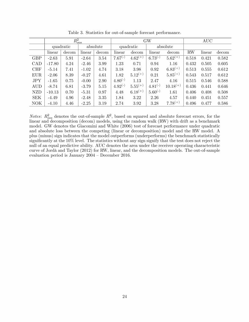
Table 3. Statistics for out-of-sample forecast performance.
R2oos GW AUCquadratic absolute quadratic absolute
linear decom linear decom linear decom linear decom RW linear decomGBP -2.63 5.91 -2.64 3.54 7.67(-) 4.62(+) 6.73(-) 5.62(+) 0.518 0.421 0.582CAD -17.80 4.24 -2.46 3.99 1.23 0.71 0.94 1.16 0.432 0.505 0.605CHF -5.14 7.41 -1.02 4.74 3.18 3.98 0.92 6.83(+) 0.513 0.555 0.612EUR -2.06 8.39 -0.27 4.61 1.82 5.12(+) 0.21 5.85(+) 0.543 0.517 0.612JPY -1.65 0.75 -0.00 2.90 4.80(-) 1.13 2.47 4.16 0.515 0.546 0.588AUD -8.74 6.81 -3.79 5.15 4.92(-) 5.55(+) 4.81(-) 10.18(+) 0.436 0.441 0.646NZD -10.13 0.70 -5.31 0.97 4.48 6.18(+) 5.60(-) 1.61 0.406 0.408 0.508SEK -4.49 4.96 -2.48 3.35 1.84 3.22 2.26 4.57 0.440 0.451 0.557NOK -4.10 4.46 -2.25 3.19 2.74 3.92 3.28 7.78(+) 0.496 0.477 0.586
Notes: R2oos denotes the out-of-sample R2, based on squared and absolute forecast errors, for the
linear and decomposition (decom) models, using the random walk (RW) with drift as a benchmarkmodel. GW denotes the Giacomini and White (2006) test of forecast performance under quadraticand absolute loss between the competing (linear or decomposition) model and the RW model. Aplus (minus) sign indicates that the model outperforms (underperforms) the benchmark statisticallysigni�cantly at the 10% level. The statistics without any sign signify that the test does not reject thenull of an equal predictive ability. AUC denotes the area under the receiver operating characteristiccurve of Jordà and Taylor (2012) for RW, linear, and the decomposition models. The out-of-sampleevaluation period is January 2004 �December 2016.
24

Table 4. Dollar values ($100 initial investment), annualized average returns, standard deviationsand Sharpe ratios of trading strategies for individual currencies.
Payo¤ in $ Average return Std. deviation Sharpe ratiobench linear decom bench linear decom bench linear decom bench linear decom
GBP 75.67 91.47 211.85 -1.85 -0.30 6.18 7.55 8.76 8.99 -0.24 -0.03 0.68CAD 72.11 75.45 111.92 -2.19 -1.71 1.33 7.97 9.51 9.71 -0.27 -0.18 0.13CHF 92.65 84.11 114.07 0.10 -0.75 3.32 10.17 10.64 10.12 0.01 -0.07 0.32EUR 115.78 93.89 205.40 1.43 -0.02 6.03 7.94 9.58 9.88 0.18 -0.00 0.61JPY 110.62 84.83 105.20 1.05 -0.77 0.87 7.52 9.89 9.73 0.14 -0.07 0.08AUD 115.00 56.23 209.41 1.93 -3.59 6.51 13.01 12.71 12.88 0.14 -0.28 0.50NZD 125.69 86.15 105.03 2.71 -0.25 1.32 13.76 13.35 13.76 0.19 -0.01 0.09SEK 86.45 53.96 149.22 -0.66 -4.12 3.67 9.58 11.11 10.93 -0.06 -0.37 0.33NOK 55.79 65.21 128.77 -3.86 -2.67 2.52 11.00 11.05 10.82 -0.35 -0.24 0.23
Notes: The table presents the dollar payo¤s to a $100 initial investment, annualized average re-turns in %, standard deviations and Sharpe ratios based on the sign of the predicted carry tradereturn from one of the competing models (benchmark (bench), linear and decomposition (decom))during the out-of-sample evaluation period: January 2004 �December 2016. Benchmark refers toa strategy of taking a long or short position depending on the sign of the forward premium.
25
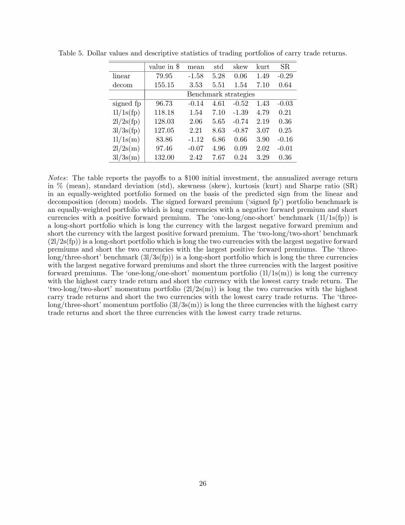
Table 5. Dollar values and descriptive statistics of trading portfolios of carry trade returns.
value in $ mean std skew kurt SRlinear 79.95 -1.58 5.28 0.06 1.49 -0.29decom 155.15 3.53 5.51 1.54 7.10 0.64
Benchmark strategiessigned fp 96.73 -0.14 4.61 -0.52 1.43 -0.031l/1s(fp) 118.18 1.54 7.10 -1.39 4.79 0.212l/2s(fp) 128.03 2.06 5.65 -0.74 2.19 0.363l/3s(fp) 127.05 2.21 8.63 -0.87 3.07 0.251l/1s(m) 83.86 -1.12 6.86 0.66 3.90 -0.162l/2s(m) 97.46 -0.07 4.96 0.09 2.02 -0.013l/3s(m) 132.00 2.42 7.67 0.24 3.29 0.36
Notes: The table reports the payo¤s to a $100 initial investment, the annualized average returnin % (mean), standard deviation (std), skewness (skew), kurtosis (kurt) and Sharpe ratio (SR)in an equally-weighted portfolio formed on the basis of the predicted sign from the linear anddecomposition (decom) models. The signed forward premium (�signed fp�) portfolio benchmark isan equally-weighted portfolio which is long currencies with a negative forward premium and shortcurrencies with a positive forward premium. The �one-long/one-short� benchmark (1l/1s(fp)) isa long-short portfolio which is long the currency with the largest negative forward premium andshort the currency with the largest positive forward premium. The �two-long/two-short�benchmark(2l/2s(fp)) is a long-short portfolio which is long the two currencies with the largest negative forwardpremiums and short the two currencies with the largest positive forward premiums. The �three-long/three-short�benchmark (3l/3s(fp)) is a long-short portfolio which is long the three currencieswith the largest negative forward premiums and short the three currencies with the largest positiveforward premiums. The �one-long/one-short�momentum portfolio (1l/1s(m)) is long the currencywith the highest carry trade return and short the currency with the lowest carry trade return. The�two-long/two-short�momentum portfolio (2l/2s(m)) is long the two currencies with the highestcarry trade returns and short the two currencies with the lowest carry trade returns. The �three-long/three-short�momentum portfolio (3l/3s(m)) is long the three currencies with the highest carrytrade returns and short the three currencies with the lowest carry trade returns.
26

Figure 1: Monthly returns for the spot exchange rates against USD (in percent).
1970 1980 1990 2000 2010 2020
-20
-10
0
10
GBP
1970 1980 1990 2000 2010 2020
-20
-10
0
10
CAD
1970 1980 1990 2000 2010 2020
-20
-10
0
10
CHF
1970 1980 1990 2000 2010 2020
-20
-10
0
10
EUR
1970 1980 1990 2000 2010 2020
-20
-10
0
10
JPY
1970 1980 1990 2000 2010 2020
-20
-10
0
10
AUD
1970 1980 1990 2000 2010 2020
-20
-10
0
10
NZD
1970 1980 1990 2000 2010 2020
-20
-10
0
10
SEK
1970 1980 1990 2000 2010 2020
-20
-10
0
10
NOK
27