Foundations of Neoclassical Growth · Foundations of Neoclassical Growth Omer Ozak SMU Macroeconomics II Omer Ozak (SMU) Economic Growth Macroeconomics II 1 / 78. Preliminaries Introduction

Foundations of Neoclassical Growth

Omer Ozak

SMU

Macroeconomics II

Omer Ozak (SMU) Economic Growth Macroeconomics II 1 / 78

Preliminaries Introduction

Foundations of Neoclassical Growth

Solow model: constant saving rate.

More satisfactory to specify the preference orderings of individualsand derive their decisions from these preferences.

Enables better understanding of the factors that affect savingsdecisions.

Enables to discuss the “optimality” of equilibria

Whether the (competitive) equilibria of growth models can be“improved upon”.

Notion of improvement: Pareto optimality.


Preliminaries Preliminaries

Preliminaries I

Consider an economy consisting of a unit measure of infinitely-livedhouseholds.

I.e., an uncountable number of households: e.g., the set of householdsH could be represented by the unit interval [0, 1].

Emphasize that each household is infinitesimal and will have no effecton aggregates.

Can alternatively think of H as a countable set of the formH = {1, 2, ...,M} with M = ∞, without any loss of generality.

Advantage of unit measure: averages and aggregates are the same

Simpler to have H as a finite set in the form {1, 2, ...,M} with Mlarge but finite.

Acceptable for many models, but with overlapping generations requirethe set of households to be infinite.



Preliminaries II

How to model households in infinite horizon?

1 “infinitely lived” or consisting of overlapping generations with fullaltruism linking generations→infinite planning horizon

2 overlapping generations→finite planning horizon (generally...).



Time Separable Preferences

Standard assumptions on preference orderings so that they can berepresented by utility functions.

In particular, each household i has an instantaneous utility function

ui (ci (t)) ,

ui : R+→ R is increasing and concave and ci (t) is the consumptionof household i .

Note instantaneous utility function is not specifying a completepreference ordering over all commodities—here consumption levels inall dates.

Sometimes also referred to as the “felicity function”.

Two major assumptions in writing an instantaneous utility function

1 consumption externalities are ruled out.2 overall utility is time separable.


Preliminaries Infinite Horizon

Infinite Planning Horizon

Start with the case of infinite planning horizon.

Suppose households discount the future “exponentially”—or“proportionally”.

Thus household preferences at time t = 0 are

Ei0

∞

∑t=0

βti ui (ci (t)) , (1)

where βi ∈ (0, 1) is the discount factor of household i .

Interpret ui (·) as a “Bernoulli utility function”.

Then preferences of household i at time t = 0 can be represented bythe following von Neumann-Morgenstern expected utility function.



Heterogeneity and the Representative Household

Ei0 is the expectation operator with respect to the information set

available to household i at time t = 0.

So far index individual utility function, ui (·), and the discount factor,βi , by “i”

Households could also differ according to their income processes.E.g., effective labor endowments of {ei (t)}∞

t=0, labor income of{ei (t)w (t)}∞

t=0.

But at this level of generality, this problem is not tractable.

Follow the standard approach in macroeconomics and assume theexistence of a representative household.



Time Consistency

Exponential discounting and time separability: ensure“time-consistent” behavior.

A solution {x (t)}Tt=0 (possibly with T = ∞) is time consistent if:

whenever {x (t)}Tt=0 is an optimal solution starting at time t = 0,

{x (t)}Tt=t ′ is an optimal solution to the continuation dynamicoptimization problem starting from time t = t ′ ∈ [0,T ].


Representative Household Representative Household

Challenges to the Representative Household

An economy admits a representative household if preference side canbe represented as if a single household made the aggregateconsumption and saving decisions subject to a single budgetconstraint.

This description concerning a representative household is purelypositive

Stronger notion of “normative” representative household: if we canalso use the utility function of the representative household for welfarecomparisons.

Simplest case that will lead to the existence of a representativehousehold: suppose each household is identical.


Representative Household Representative Household

Representative Household II

I.e., same β, same sequence {e (t)}∞t=0 and same

u (ci (t))

where u : R+→ R is increasing and concave and ci (t) is theconsumption of household i .

Again ignoring uncertainty, preference side can be represented as thesolution to

max∞

∑t=0

βtu (c (t)) , (2)

β ∈ (0, 1) is the common discount factor and c (t) the consumptionlevel of the representative household.

Admits a representative household rather trivially.

Representative household’s preferences, (2), can be used for positiveand normative analysis.


Representative Household A Negative Result

Representative Household III

If instead households are not identical but assume can model as ifdemand side generated by the optimization decision of arepresentative household:More realistic, but:

1 The representative household will have positive, but not always anormative meaning.

2 Models with heterogeneity: often not lead to behavior that can berepresented as if generated by a representative household.

Theorem (Debreu-Mantel-Sonnenschein Theorem) Let ε > 0 be ascalar and N < ∞ be a positive integer. Consider a set ofprices P ε =

{p ∈ RN

+: pj/pj ′ ≥ ε for all j and j ′}

and anycontinuous function x : P ε → RN

+ that satisfies Walras’ Lawand is homogeneous of degree 0. Then there exists anexchange economy with N commodities and H < ∞households, where the aggregate demand is given by x (p)over the set P ε.


Representative Household A Negative Result

Representative Household IV

That excess demands come from optimizing behavior of householdsputs no restrictions on the form of these demands.

E.g., x (p) does not necessarily possess a negative-semi-definiteJacobian or satisfy the weak axiom of revealed preference(requirements of demands generated by individual households).

Hence without imposing further structure, impossible to derivespecific x (p)’s from the maximization behavior of a single household.

Severe warning against the use of the representative householdassumption.

Partly an outcome of very strong income effects:

special but approximately realistic preference functions, and restrictionson distribution of income rule out arbitrary aggregate excess demandfunctions.


Representative Household A Partial Positive Result

Gorman Aggregation

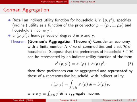
Recall an indirect utility function for household i , vi(p, y i

), specifies

(ordinal) utility as a function of the price vector p = (p1, ..., pN) andhousehold’s income y i .vi(p, y i

): homogeneous of degree 0 in p and y .

Theorem (Gorman’s Aggregation Theorem) Consider an economywith a finite number N < ∞ of commodities and a set H ofhouseholds. Suppose that the preferences of household i ∈ Hcan be represented by an indirect utility function of the form

v i(p, y i

)= ai (p) + b (p) y i , (3)

then these preferences can be aggregated and represented bythose of a representative household, with indirect utility

v (p, y) =∫i∈H

ai (p) di + b (p) y ,

where y ≡∫i∈H y idi is aggregate income.



Linear Engel Curves

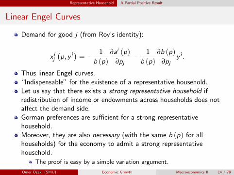
Demand for good j (from Roy’s identity):

x ij(p, y i

)= − 1

b (p)

∂ai (p)

∂pj− 1

b (p)

∂b (p)

∂pjy i .

Thus linear Engel curves.

“Indispensable” for the existence of a representative household.

Let us say that there exists a strong representative household ifredistribution of income or endowments across households does notaffect the demand side.

Gorman preferences are sufficient for a strong representativehousehold.

Moreover, they are also necessary (with the same b (p) for allhouseholds) for the economy to admit a strong representativehousehold.

The proof is easy by a simple variation argument.



Importance of Gorman Preferences

Gorman Preferences limit the extent of income effects and enablesthe aggregation of individual behavior.

Integral is “Lebesgue integral,” so when H is a finite or countable set,∫i∈H y idi is indeed equivalent to the summation ∑i∈H y i .

Stated for an economy with a finite number of commodities, but canbe generalized for infinite or even a continuum of commodities.

Note all we require is there exists a monotonic transformation of theindirect utility function that takes the form in (3)—as long as nouncertainty.

Contains some commonly-used preferences in macroeconomics.



Example: Constant Elasticity of Substitution Preferences

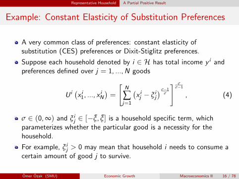
A very common class of preferences: constant elasticity ofsubstitution (CES) preferences or Dixit-Stiglitz preferences.

Suppose each household denoted by i ∈ H has total income y i andpreferences defined over j = 1, ...,N goods

U i(x i1, ..., x iN

)=

[N

∑j=1

(x ij − ξ ij

) σ−1σ

] σσ−1

, (4)

σ ∈ (0, ∞) and ξ ij ∈ [−ξ, ξ] is a household specific term, whichparameterizes whether the particular good is a necessity for thehousehold.

For example, ξ ij > 0 may mean that household i needs to consume acertain amount of good j to survive.



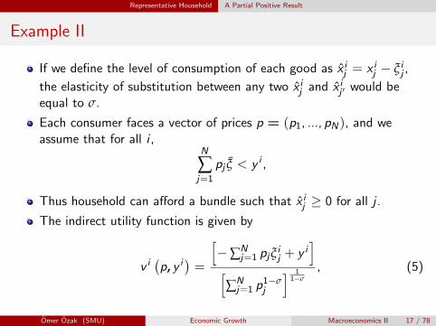
Example II

If we define the level of consumption of each good as x ij = x ij − ξ ij ,

the elasticity of substitution between any two x ij and x ij ′ would beequal to σ.

Each consumer faces a vector of prices p = (p1, ..., pN), and weassume that for all i ,

N

∑j=1

pj ξ < y i ,

Thus household can afford a bundle such that x ij ≥ 0 for all j .

The indirect utility function is given by

v i(p, y i

)=

[−∑N

j=1 pjξij + y i

][∑N

j=1 p1−σj

] 11−σ

, (5)



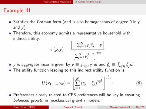
Example III

Satisfies the Gorman form (and is also homogeneous of degree 0 in pand y).

Therefore, this economy admits a representative household withindirect utility:

v (p, y) =

[−∑N

j=1 pjξj + y]

[∑N

j=1 p1−σj

] 11−σ

y is aggregate income given by y ≡∫i∈H y idi and ξj ≡

∫i∈H ξ ijdi .

The utility function leading to this indirect utility function is

U (x1, ..., xN) =

[N

∑j=1

(xj − ξj )σ−1

σ

] σσ−1

. (6)

Preferences closely related to CES preferences will be key in ensuringbalanced growth in neoclassical growth models.


Representative Household Normative Representative Household

Normative Representative Household

Gorman preferences also imply the existence of a normativerepresentative household.

Recall an allocation is Pareto optimal if no household can be madestrictly better-off without some other household being made worse-off.



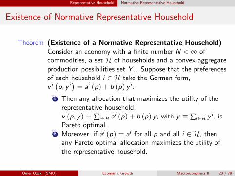
Existence of Normative Representative Household

Theorem (Existence of a Normative Representative Household)Consider an economy with a finite number N < ∞ ofcommodities, a set H of households and a convex aggregateproduction possibilities set Y .. Suppose that the preferencesof each household i ∈ H take the Gorman form,v i(p, y i

)= ai (p) + b (p) y i .

1 Then any allocation that maximizes the utility of therepresentative household,v (p, y) = ∑i∈H ai (p) + b (p) y , with y ≡ ∑i∈H y i , isPareto optimal.

2 Moreover, if ai (p) = ai for all p and all i ∈ H, thenany Pareto optimal allocation maximizes the utility ofthe representative household.



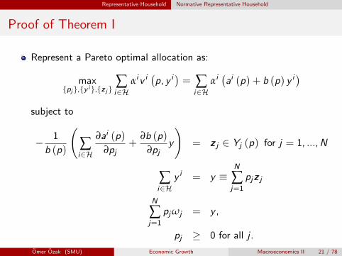
Proof of Theorem I

Represent a Pareto optimal allocation as:

max{pj},{y i},{z j}

∑i∈H

αiv i(p, y i

)= ∑

i∈Hαi(ai (p) + b (p) y i

)subject to

− 1

b (p)

(∑i∈H

∂ai (p)

∂pj+

∂b (p)

∂pjy

)= z j ∈ Yj (p) for j = 1, ...,N

∑i∈H

y i = y ≡N

∑j=1

pjz j

N

∑j=1

pjωj = y ,

pj ≥ 0 for all j .



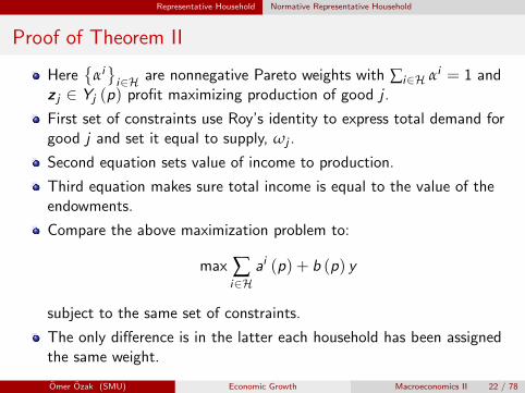
Proof of Theorem II

Here{

αi}i∈H are nonnegative Pareto weights with ∑i∈H αi = 1 and

z j ∈ Yj (p) profit maximizing production of good j .

First set of constraints use Roy’s identity to express total demand forgood j and set it equal to supply, ωj .

Second equation sets value of income to production.

Third equation makes sure total income is equal to the value of theendowments.

Compare the above maximization problem to:

max ∑i∈H

ai (p) + b (p) y

subject to the same set of constraints.

The only difference is in the latter each household has been assignedthe same weight.



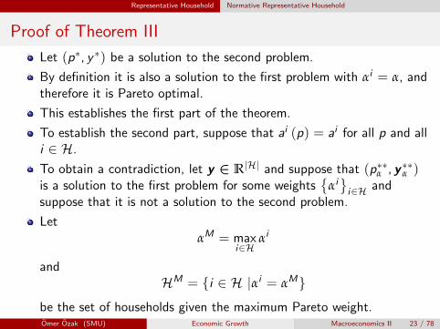
Proof of Theorem III

Let (p∗, y ∗) be a solution to the second problem.

By definition it is also a solution to the first problem with αi = α, andtherefore it is Pareto optimal.

This establishes the first part of the theorem.

To establish the second part, suppose that ai (p) = ai for all p and alli ∈ H.

To obtain a contradiction, let y ∈ R|H| and suppose that (p∗∗α , y ∗∗α )is a solution to the first problem for some weights

{αi}i∈H and

suppose that it is not a solution to the second problem.

LetαM = max

i∈Hαi

andHM = {i ∈ H |αi = αM}

be the set of households given the maximum Pareto weight.Omer Ozak (SMU) Economic Growth Macroeconomics II 23 / 78


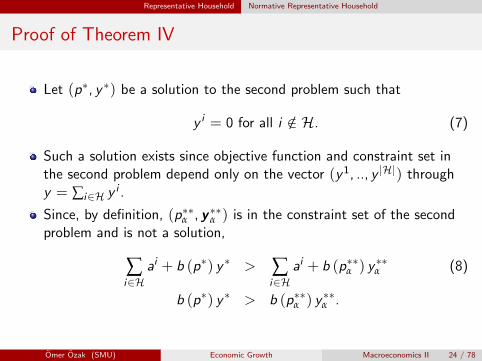
Proof of Theorem IV

Let (p∗, y ∗) be a solution to the second problem such that

y i = 0 for all i /∈ H. (7)

Such a solution exists since objective function and constraint set inthe second problem depend only on the vector (y1, .., y |H|) throughy = ∑i∈H y i .

Since, by definition, (p∗∗α , y ∗∗α ) is in the constraint set of the secondproblem and is not a solution,

∑i∈H

ai + b (p∗) y ∗ > ∑i∈H

ai + b (p∗∗α ) y ∗∗α (8)

b (p∗) y ∗ > b (p∗∗α ) y ∗∗α .



Proof of Theorem V

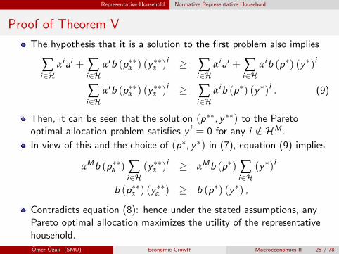
The hypothesis that it is a solution to the first problem also implies

∑i∈H

αiai + ∑i∈H

αib (p∗∗α ) (y ∗∗α )i ≥ ∑i∈H

αiai + ∑i∈H

αib (p∗) (y ∗)i

∑i∈H

αib (p∗∗α ) (y ∗∗α )i ≥ ∑i∈H

αib (p∗) (y ∗)i . (9)

Then, it can be seen that the solution (p∗∗, y ∗∗) to the Paretooptimal allocation problem satisfies y i = 0 for any i /∈ HM .

In view of this and the choice of (p∗, y ∗) in (7), equation (9) implies

αMb (p∗∗α ) ∑i∈H

(y ∗∗α )i ≥ αMb (p∗) ∑i∈H

(y ∗)i

b (p∗∗α ) (y ∗∗α ) ≥ b (p∗) (y ∗) ,

Contradicts equation (8): hence under the stated assumptions, anyPareto optimal allocation maximizes the utility of the representativehousehold.


Infinite Planning Horizon Infinite Horizon

Infinite Planning Horizon I

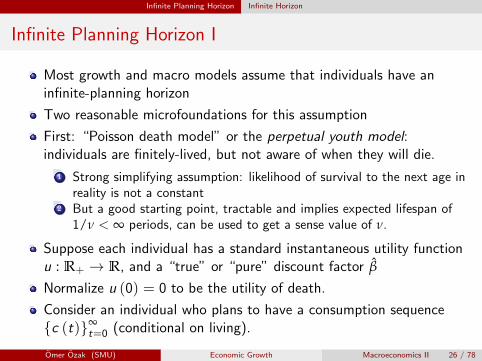
Most growth and macro models assume that individuals have aninfinite-planning horizon

Two reasonable microfoundations for this assumption

First: “Poisson death model” or the perpetual youth model:individuals are finitely-lived, but not aware of when they will die.

1 Strong simplifying assumption: likelihood of survival to the next age inreality is not a constant

2 But a good starting point, tractable and implies expected lifespan of1/ν < ∞ periods, can be used to get a sense value of ν.

Suppose each individual has a standard instantaneous utility functionu : R+ → R, and a “true” or “pure” discount factor β

Normalize u (0) = 0 to be the utility of death.

Consider an individual who plans to have a consumption sequence{c (t)}∞

t=0 (conditional on living).



Infinite Planning Horizon II

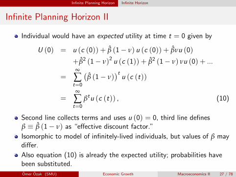
Individual would have an expected utility at time t = 0 given by

U (0) = u (c (0)) + β (1− ν) u (c (0)) + βνu (0)

+β2 (1− ν)2 u (c (1)) + β2 (1− ν) νu (0) + ...

=∞

∑t=0

(β (1− ν)

)tu (c (t))

=∞

∑t=0

βtu (c (t)) , (10)

Second line collects terms and uses u (0) = 0, third line definesβ ≡ β (1− ν) as “effective discount factor.”

Isomorphic to model of infinitely-lived individuals, but values of β maydiffer.

Also equation (10) is already the expected utility; probabilities havebeen substituted.



Infinite Planning Horizon III

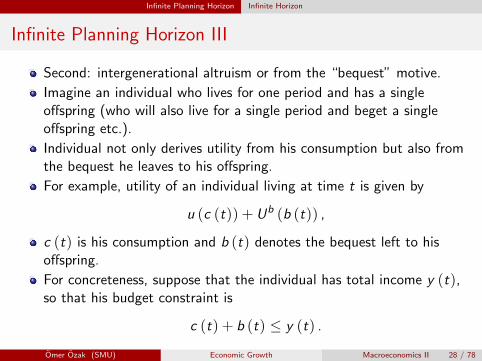
Second: intergenerational altruism or from the “bequest” motive.

Imagine an individual who lives for one period and has a singleoffspring (who will also live for a single period and beget a singleoffspring etc.).

Individual not only derives utility from his consumption but also fromthe bequest he leaves to his offspring.

For example, utility of an individual living at time t is given by

u (c (t)) + Ub (b (t)) ,

c (t) is his consumption and b (t) denotes the bequest left to hisoffspring.

For concreteness, suppose that the individual has total income y (t),so that his budget constraint is

c (t) + b (t) ≤ y (t) .



Infinite Planning Horizon IV

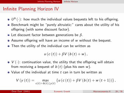
Ub (·): how much the individual values bequests left to his offspring.

Benchmark might be “purely altruistic:” cares about the utility of hisoffspring (with some discount factor).

Let discount factor between generations be β.

Assume offspring will have an income of w without the bequest.

Then the utility of the individual can be written as

u (c (t)) + βV (b (t) + w) ,

V (·): continuation value, the utility that the offspring will obtainfrom receiving a bequest of b (t) (plus his own w).

Value of the individual at time t can in turn be written as

V (y (t)) = maxc(t)+b(t)≤y (t)

{u (c (t)) + βV (b (t) + w (t + 1))} ,



Infinite Planning Horizon V

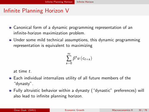
Canonical form of a dynamic programming representation of aninfinite-horizon maximization problem.

Under some mild technical assumptions, this dynamic programmingrepresentation is equivalent to maximizing

∞

∑s=0

βsu (ct+s)

at time t.

Each individual internalizes utility of all future members of the“dynasty”.

Fully altruistic behavior within a dynasty (“dynastic” preferences) willalso lead to infinite planning horizon.


Representative Firm Representative Firm

The Representative Firm I

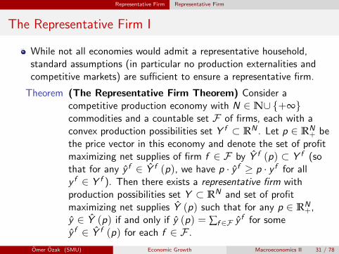
While not all economies would admit a representative household,standard assumptions (in particular no production externalities andcompetitive markets) are sufficient to ensure a representative firm.

Theorem (The Representative Firm Theorem) Consider acompetitive production economy with N ∈N∪ {+∞}commodities and a countable set F of firms, each with aconvex production possibilities set Y f ⊂ RN . Let p ∈ RN

+ bethe price vector in this economy and denote the set of profitmaximizing net supplies of firm f ∈ F by Y f (p) ⊂ Y f (sothat for any y f ∈ Y f (p), we have p · y f ≥ p · y f for ally f ∈ Y f ). Then there exists a representative firm withproduction possibilities set Y ⊂ RN and set of profitmaximizing net supplies Y (p) such that for any p ∈ RN

+,y ∈ Y (p) if and only if y (p) = ∑f ∈F y f for somey f ∈ Y f (p) for each f ∈ F .



Proof of Theorem: The Representative Firm I

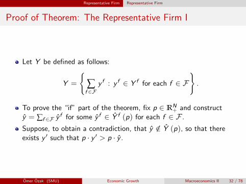
Let Y be defined as follows:

Y =

{∑f ∈F

y f : y f ∈ Y f for each f ∈ F}

.

To prove the “if” part of the theorem, fix p ∈ RN+ and construct

y = ∑f ∈F y f for some y f ∈ Y f (p) for each f ∈ F .

Suppose, to obtain a contradiction, that y /∈ Y (p), so that thereexists y ′ such that p · y ′ > p · y .



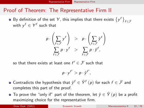
Proof of Theorem: The Representative Firm II

By definition of the set Y , this implies that there exists{y f}f ∈F

with y f ∈ Y f such that

p ·(

∑f ∈F

y f

)> p ·

(∑f ∈F

y f

)∑f ∈F

p · y f > ∑f ∈F

p · y f ,

so that there exists at least one f ′ ∈ F such that

p · y f ′ > p · y f ′ ,

Contradicts the hypothesis that y f ∈ Y f (p) for each f ∈ F andcompletes this part of the proof.

To prove the “only if” part of the theorem, let y ∈ Y (p) be a profitmaximizing choice for the representative firm.



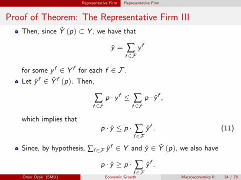
Proof of Theorem: The Representative Firm III

Then, since Y (p) ⊂ Y , we have that

y = ∑f ∈F

y f

for some y f ∈ Y f for each f ∈ F .

Let y f ∈ Y f (p). Then,

∑f ∈F

p · y f ≤ ∑f ∈F

p · y f ,

which implies thatp · y ≤ p · ∑

f ∈Fy f . (11)

Since, by hypothesis, ∑f ∈F y f ∈ Y and y ∈ Y (p), we also have

p · y ≥ p · ∑f ∈F

y f .



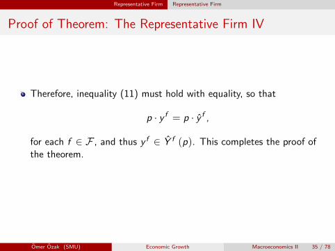
Proof of Theorem: The Representative Firm IV

Therefore, inequality (11) must hold with equality, so that

p · y f = p · y f ,

for each f ∈ F , and thus y f ∈ Y f (p). This completes the proof ofthe theorem.



The Representative Firm II

Why such a difference between representative household andrepresentative firm assumptions? Income effects.

Changes in prices create income effects, which affect differenthouseholds differently.

No income effects in producer theory, so the representative firmassumption is without loss of any generality.

Does not mean that heterogeneity among firms is uninteresting orunimportant.

Many models of endogenous technology feature productivitydifferences across firms, and firms’ attempts to increase theirproductivity relative to others will often be an engine of economicgrowth.


Optimal Growth Problem Formulation

Problem Formulation I

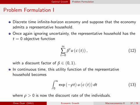
Discrete time infinite-horizon economy and suppose that the economyadmits a representative household.

Once again ignoring uncertainty, the representative household has thet = 0 objective function

∞

∑t=0

βtu (c (t)) , (12)

with a discount factor of β ∈ (0, 1).

In continuous time, this utility function of the representativehousehold becomes ∫ ∞

0exp (−ρt) u (c (t)) dt (13)

where ρ > 0 is now the discount rate of the individuals.



Problem Formulation II

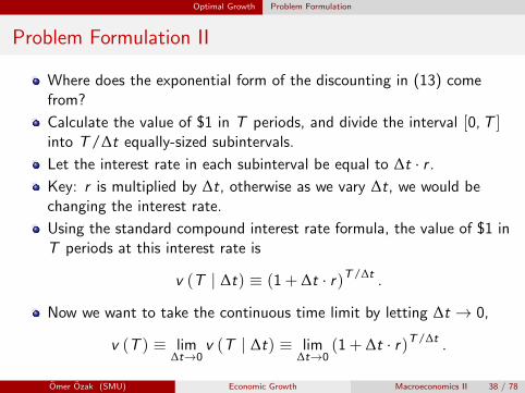
Where does the exponential form of the discounting in (13) comefrom?

Calculate the value of $1 in T periods, and divide the interval [0,T ]into T/∆t equally-sized subintervals.

Let the interest rate in each subinterval be equal to ∆t · r .

Key: r is multiplied by ∆t, otherwise as we vary ∆t, we would bechanging the interest rate.

Using the standard compound interest rate formula, the value of $1 inT periods at this interest rate is

v (T | ∆t) ≡ (1 + ∆t · r)T/∆t .

Now we want to take the continuous time limit by letting ∆t → 0,

v (T ) ≡ lim∆t→0

v (T | ∆t) ≡ lim∆t→0

(1 + ∆t · r)T/∆t .



Problem Formulation III

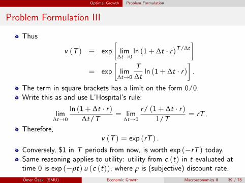
Thus

v (T ) ≡ exp

[lim

∆t→0ln (1 + ∆t · r)T/∆t

]= exp

[lim

∆t→0

T

∆tln (1 + ∆t · r)

].

The term in square brackets has a limit on the form 0/0.

Write this as and use L’Hospital’s rule:

lim∆t→0

ln (1 + ∆t · r)∆t/T

= lim∆t→0

r/ (1 + ∆t · r)1/T

= rT ,

Therefore,v (T ) = exp (rT ) .

Conversely, $1 in T periods from now, is worth exp (−rT ) today.

Same reasoning applies to utility: utility from c (t) in t evaluated attime 0 is exp (−ρt) u (c (t)), where ρ is (subjective) discount rate.


Welfare Theorems Towards Equilibrium

Welfare Theorems I

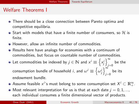
There should be a close connection between Pareto optima andcompetitive equilibria.

Start with models that have a finite number of consumers, so H isfinite.

However, allow an infinite number of commodities.

Results here have analogs for economies with a continuum ofcommodities, but focus on countable number of commodities.

Let commodities be indexed by j ∈N and x i ≡{x ij

}∞

j=0be the

consumption bundle of household i , and ωi ≡{

ωij

}∞

j=0be its

endowment bundle.

Assume feasible x i ’s must belong to some consumption set X i ⊂ R∞+ .

Most relevant interpretation for us is that at each date j = 0, 1, ...,each individual consumes a finite dimensional vector of products.



Welfare Theorems II

Thus x ij ∈ X ij ⊂ RK

+ for some integer K .

Consumption set introduced to allow cases where individual may nothave negative consumption of certain commodities.

Let X ≡ ∏i∈H X i be the Cartesian product of these consumptionsets, the aggregate consumption set of the economy.

Also use the notation x ≡{x i}i∈H and ω ≡

{ωi}i∈H to describe

the entire consumption allocation and endowments in the economy.

Feasibility requires that x ∈ X .

Each household in H has a well defined preference ordering overconsumption bundles.

This preference ordering can be represented by a relationship %i forhousehold i , such that x ′ %i x implies that household i weakly prefersx ′ to x .



Welfare Theorems III

Suppose that preferences can be represented by ui : X i → R, suchthat whenever x ′ %i x , we have ui (x ′) ≥ ui (x).

The domain of this function is X i ⊂ R∞+ .

Let u ≡{ui}i∈H be the set of utility functions.

Production side: finite number of firms represented by FEach firm f ∈ F is characterized by production set Y f , specifieslevels of output firm f can produce from specified levels of inputs.

I.e., y f ≡{y fj

}∞

j=0is a feasible production plan for firm f if y f ∈ Y f .

E.g., if there were only labor and a final good, Y f would include pairs(−l , y) such that with labor input l the firm can produce at most y .



Welfare Theorems IV

Take each Y f to be a cone, so that if y ∈ Y f , then λy ∈ Y f for anyλ ∈ R+. This implies:

1 0 ∈ Y f for each f ∈ F ;2 each Y f exhibits constant returns to scale.

If there are diminishing returns to scale from some scarce factors, thisis added as an additional factor of production and Y f is still a cone.

Let Y ≡ ∏f ∈F Y f represent the aggregate production set andy ≡

{y f}f ∈F such that y f ∈ Y f for all f , or equivalently, y ∈ Y .

Ownership structure of firms: if firms make profits, they should bedistributed to some agents

Assume there exists a sequence of numbers (profit shares)θ≡

{θif}f ∈F ,i∈H such that θif ≥ 0 for all f and i , and ∑i∈H θif = 1

for all f ∈ F .

θif is the share of profits of firm f that will accrue to household i .



Welfare Theorems V

An economy E is described by E ≡ (H,F , u, ω, Y , X , θ).

An allocation is (x , y ) such that x and y are feasible, that is, x ∈ X ,y ∈ Y , and ∑i∈H x ij ≤ ∑i∈H ωi

j + ∑f ∈F y fj for all j ∈N.

A price system is a sequence p ≡ {pj}∞j=0, such that pj ≥ 0 for all j .

We can choose one of these prices as the numeraire and normalize itto 1.

Also define p · x as the inner product of p and x , i.e.,p · x ≡ ∑∞

j=0 pjxj .



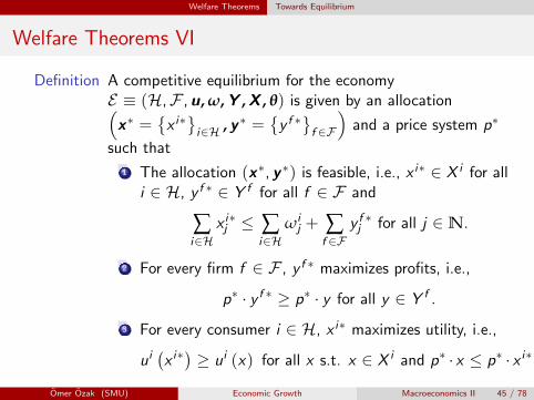
Welfare Theorems VI

Definition A competitive equilibrium for the economyE ≡ (H,F , u, ω, Y , X , θ) is given by an allocation(x∗ =

{x i∗}i∈H , y ∗ =

{y f ∗}f ∈F

)and a price system p∗

such that

1 The allocation (x∗, y ∗) is feasible, i.e., x i∗ ∈ X i for alli ∈ H, y f ∗ ∈ Y f for all f ∈ F and

∑i∈H

x i∗j ≤ ∑i∈H

ωij + ∑

f ∈Fy f ∗j for all j ∈N.

2 For every firm f ∈ F , y f ∗ maximizes profits, i.e.,

p∗ · y f ∗ ≥ p∗ · y for all y ∈ Y f .

3 For every consumer i ∈ H, x i∗ maximizes utility, i.e.,

ui(x i∗)≥ ui (x) for all x s.t. x ∈ X i and p∗ · x ≤ p∗ · x i∗.



Welfare Theorems VII

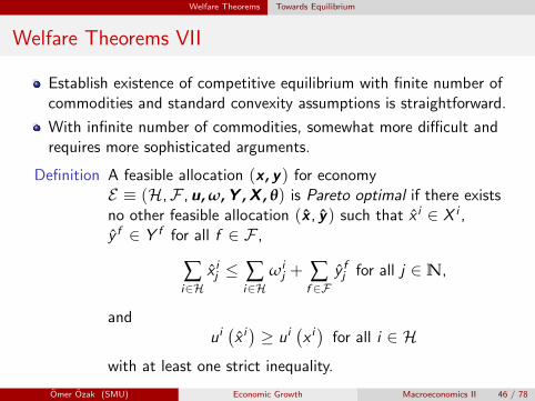
Establish existence of competitive equilibrium with finite number ofcommodities and standard convexity assumptions is straightforward.

With infinite number of commodities, somewhat more difficult andrequires more sophisticated arguments.

Definition A feasible allocation (x , y ) for economyE ≡ (H,F , u, ω, Y , X , θ) is Pareto optimal if there existsno other feasible allocation (x , y ) such that x i ∈ X i ,y f ∈ Y f for all f ∈ F ,

∑i∈H

x ij ≤ ∑i∈H

ωij + ∑

f ∈Fy fj for all j ∈N,

andui(x i)≥ ui

(x i)

for all i ∈ H

with at least one strict inequality.



Welfare Theorems VIII

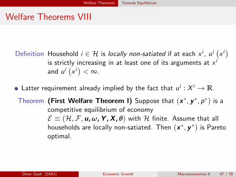
Definition Household i ∈ H is locally non-satiated if at each x i , ui(x i)

is strictly increasing in at least one of its arguments at x i

and ui(x i)< ∞.

Latter requirement already implied by the fact that ui : X i → R.

Theorem (First Welfare Theorem I) Suppose that (x∗, y ∗, p∗) is acompetitive equilibrium of economyE ≡ (H,F , u, ω, Y , X , θ) with H finite. Assume that allhouseholds are locally non-satiated. Then (x∗, y ∗) is Paretooptimal.



Proof of First Welfare Theorem I

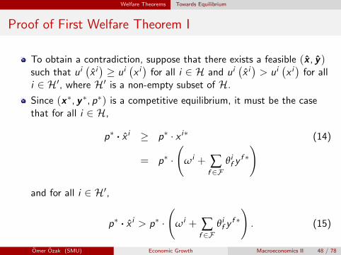
To obtain a contradiction, suppose that there exists a feasible (x , y )such that ui

(x i)≥ ui

(x i)

for all i ∈ H and ui(x i)> ui

(x i)

for alli ∈ H′, where H′ is a non-empty subset of H.

Since (x∗, y ∗, p∗) is a competitive equilibrium, it must be the casethat for all i ∈ H,

p∗ · x i ≥ p∗ · x i∗ (14)

= p∗ ·(

ωi + ∑f ∈F

θif yf ∗)

and for all i ∈ H′,

p∗ · x i > p∗ ·(

ωi + ∑f ∈F

θif yf ∗)

. (15)



Proof of First Welfare Theorem II

Second inequality follows immediately in view of the fact that x i∗ isthe utility maximizing choice for household i , thus if x i is strictlypreferred, then it cannot be in the budget set.

First inequality follows with a similar reasoning. Suppose that it didnot hold.

Then by the hypothesis of local-satiation, ui must be strictlyincreasing in at least one of its arguments, let us say the j ′thcomponent of x .

Then construct x i (ε) such that x ij (ε) = x ij and x ij ′ (ε) = x ij ′ + ε.

For ε ↓ 0, x i (ε) is in household i ’s budget set and yields strictlygreater utility than the original consumption bundle x i , contradictingthe hypothesis that household i was maximizing utility.

Note local non-satiation implies that ui(x i)< ∞, and thus the

right-hand sides of (14) and (15) are finite.



Proof of First Welfare Theorem III

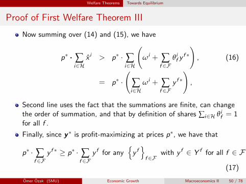
Now summing over (14) and (15), we have

p∗ · ∑i∈H

x i > p∗ · ∑i∈H

(ωi + ∑

f ∈Fθif y

f ∗)

, (16)

= p∗ ·(

∑i∈H

ωi + ∑f ∈F

y f ∗)

,

Second line uses the fact that the summations are finite, can changethe order of summation, and that by definition of shares ∑i∈H θif = 1for all f .

Finally, since y ∗ is profit-maximizing at prices p∗, we have that

p∗ · ∑f ∈F

y f ∗ ≥ p∗ · ∑f ∈F

y f for any{y f}f ∈F

with y f ∈ Y f for all f ∈ F .

(17)



Proof of First Welfare Theorem IV

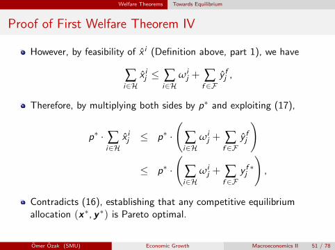
However, by feasibility of x i (Definition above, part 1), we have

∑i∈H

x ij ≤ ∑i∈H

ωij + ∑

f ∈Fy fj ,

Therefore, by multiplying both sides by p∗ and exploiting (17),

p∗ · ∑i∈H

x ij ≤ p∗ ·(

∑i∈H

ωij + ∑

f ∈Fy fj

)

≤ p∗ ·(

∑i∈H

ωij + ∑

f ∈Fy f ∗j

),

Contradicts (16), establishing that any competitive equilibriumallocation (x∗, y ∗) is Pareto optimal.



Welfare Theorems IX

Proof of the First Welfare Theorem based on two intuitive ideas.

1 If another allocation Pareto dominates the competitive equilibrium,then it must be non-affordable in the competitive equilibrium.

2 Profit-maximization implies that any competitive equilibrium alreadycontains the maximal set of affordable allocations.

Note it makes no convexity assumption.

Also highlights the importance of the feature that the relevant sumsexist and are finite.

Otherwise, the last step would lead to the conclusion that “∞ < ∞”.

That these sums exist followed from two assumptions: finiteness ofthe number of individuals and non-satiation.



Welfare Theorems X

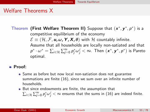
Theorem (First Welfare Theorem II) Suppose that (x∗, y ∗, p∗) is acompetitive equilibrium of the economyE ≡ (H,F , u, ω, Y , X , θ) with H countably infinite.Assume that all households are locally non-satiated and thatp∗ ·ω∗ = ∑i∈H ∑∞

j=0 p∗j ωi

j < ∞. Then (x∗, y ∗, p∗) is Paretooptimal.

Proof:

Same as before but now local non-satiation does not guaranteesummations are finite (16), since we sum over an infinite number ofhouseholds.But since endowments are finite, the assumption that

∑i∈H ∑∞j=0 p

∗j ωi

j < ∞ ensures that the sums in (16) are indeed finite.



Welfare Theorems X

Second Welfare Theorem (converse to First): whether or not H isfinite is not as important as for the First Welfare Theorem.

But requires assumptions such as the convexity of consumption andproduction sets and preferences, and additional requirements becauseit contains an “existence of equilibrium argument”.

Recall that the consumption set of each individual i ∈ H is X i ⊂ R∞+ .

A typical element of X i is x i =(x i1, x i2, ...

), where x it can be

interpreted as the vector of consumption of individual i at time t.

Similarly, a typical element of the production set of firm f ∈ F , Y f ,is y f =

(y f1 , y f2 , ...

).

Let us define x i [T ] =(x i0, x i1, x i2, ..., x iT , 0, 0, ...

)and

y f [T ] =(y f0 , y f1 , y f2 , ..., y fT , 0, 0, ...

).

It can be verified that limT→∞ x i [T ] = x i and limT→∞ y f [T ] = y f

in the product topology.



Second Welfare Theorem I

Theorem

Consider a Pareto optimal allocation (x∗∗, y ∗∗) in an economy describedby ω,

{Y f}f ∈F ,

{X i}i∈H, and

{ui (·)

}i∈H. Suppose all production and

consumption sets are convex, all production sets are cones, and all{ui (·)

}i∈H are continuous and quasi-concave and satisfy local

non-satiation. Suppose also that 0 ∈ X i , that for each x , x ′ ∈ X i withui (x) > ui (x ′) for all i ∈ H, there exists T such that ui (x [T ]) > ui (x ′)for all T ≥ T and for all i ∈ H, and that for each y ∈ Y f , there exists Tsuch that y [T ] ∈ Y f for all T ≥ T and for all f ∈ F .Then this allocationcan be decentralized as a competitive equilibrium.



Second Welfare Theorem II

Theorem

(continued) In particular, there exist p∗∗ and (ω∗∗, θ∗∗) such that

1 ω∗∗ satisfies ω = ∑i∈H ωi∗∗;

2 for all f ∈ F ,

p∗∗ · y f ∗∗ ≥ p∗∗ · y for all y ∈ Y f ;

3 for all i ∈ H,

if x i ∈ X i involves ui(x i)> ui

(x i∗∗

), then p∗∗ · x i ≥ p∗∗ · w i∗∗,

where w i∗∗ ≡ ωi∗∗ + ∑f ∈F θi∗∗f y f ∗∗.

Moreover, if p∗∗ ·w ∗∗ > 0 [i.e., p∗∗ · w i∗∗ > 0 for each i ∈ H], theneconomy E has a competitive equilibrium (x∗∗, y ∗∗, p∗∗).



Welfare Theorems XII

Notice:

if instead we had a finite commodity space, say with K commodities,then the hypothesis that 0 ∈ X i for each i ∈ H and x , x ′ ∈ X i withui (x) > ui (x ′), there exists T such that ui (x [T ]) > ui (x ′ [T ]) forall T ≥ T and all i ∈ H (and also that there exists T such that ify ∈ Y f , then y [T ] ∈ Y f for all T ≥ T and all f ∈ F) would besatisfied automatically, by taking T = T = K .Condition not imposed in Second Welfare Theorem in economies with afinite number of commodities.In dynamic economies, its role is to ensure that changes in allocationsat very far in the future should not have a large effect.

The conditions for the Second Welfare Theorem are more difficult tosatisfy than those for the First.

Also the more important of the two theorems: stronger results thatany Pareto optimal allocation can be decentralized.



Welfare Theorems XIII

Immediate corollary is an existence result: a competitive equilibriummust exist.

Motivates many to look for the set of Pareto optimal allocationsinstead of explicitly characterizing competitive equilibria.

Real power of the Theorem in dynamic macro models comes when wecombine it with models that admit a representative household.

Enables us to characterize the optimal growth allocation thatmaximizes the utility of the representative household and assert thatthis will correspond to a competitive equilibrium.


Welfare Theorems Sketch of the Proof

Sketch of the Proof of SWT I

First, I establish that there exists a price vector p∗∗ and anendowment and share allocation (ω∗∗, θ∗∗) that satisfy conditions1-3.

This has two parts.

(Part 1) This part follows from the Geometric Hahn-Banach Theorem.

Define the “more preferred” sets for each i ∈ H:

P i ={x i ∈ X i :ui

(x i)> ui

(x i∗∗

)}.

Clearly, each P i is convex.

Let P = ∑i∈H P i and Y ′ = ∑f ∈F Y f + {ω}, where recall thatω = ∑i∈H ωi∗∗, so that Y ′ is the sum of the production sets shiftedby the endowment vector.

Both P and Y ′ are convex (since each P i and each Y f are convex).



Sketch of the Proof of SWT II

Consider the sequences of production plans for each firm to be subsetsof `K∞, i.e., vectors of the form y f =

(y f0 , y f1 , ...

), with each y fj ∈ RK

+.

Moreover, since each production set is a cone, Y ′ = ∑f ∈F Y f + {ω}has an interior point.

Moreover, let x∗∗ = ∑i∈H x i∗∗.

By feasibility and local non-satiation, x∗∗ = ∑f ∈F y i∗∗ + ω.

Then x∗∗ ∈ Y ′ and also x∗∗ ∈ P (where P is the closure of P).

Next, observe that P ∩ Y ′ = ∅. Otherwise, there would exist y ∈ Y ′,which is also in P.

This implies that if distributed appropriately across the households, ywould make all households equally well off and at least one of themwould be strictly better off



Sketch of the Proof of SWT III

I.e., by the definition of the set P, there would exist{x i}i∈H such

that ∑i∈H x i = y , x i ∈ X i , and ui(x i)≥ ui

(x i∗∗

)for all i ∈ H

with at least one strict inequality.

This would contradict the hypothesis that (x∗∗, y ∗∗) is a Paretooptimum.

Since Y ′ has an interior point, P and Y ′ are convex, andP ∩ Y ′ = ∅, Geometric Theorem implies that there exists a nonzerocontinuous linear functional φ such that

φ (y) ≤ φ (x∗∗) ≤ φ (x) for all y ∈ Y ′ and all x ∈ P. (18)

(Part 2) We next need to show that this linear functional can beinterpreted as a price vector (i.e., that it does have an inner productrepresentation).



Sketch of the Proof of SWT IV

To do this, first note that if φ (x) is a continuous linear functional,then φ (x) = ∑∞

j=0 φj (xj ) is also a linear functional, where each

φj (xj ) is a linear functional on Xj ⊂ RK+.

Moreover, φ (x) = limT→∞ φ (x [T ]).

Second claim follows from the fact that φ (x [T ]) is bounded aboveby ‖φ‖ · ‖x‖, where ‖φ‖ denotes the norm of the functional φ and isthus finite.

Clearly, ‖x‖ is also finite.

Moreover, since each element of x is nonnegative, {φ (x [t])} is amonotone sequence, thus limT→∞ φ (x [T ]) converges and we denotethe limit by φ (x).

Moreover, this limit is a bounded functional and therefore fromContinuity of Linear Function Theorem, it is continuous.



Sketch of the Proof of SWT V

The first claim follows from the fact that since xj ∈ Xj ⊂ RK+, we can

define a continuous linear functional on the dual of Xj byφj (xj ) = φ

(x j)= ∑K

s=1 p∗∗j ,sxj ,s , where x j = (0, 0, ..., xj , 0, ...) [i.e., x j

has xj as jth element and zeros everywhere else].

Then clearly,

φ (x) =∞

∑j=0

φj (xj ) =∞

∑s=0

p∗∗s xs = p∗∗ · x .

To complete this part of the proof, we only need to show thatφ (x) = ∑∞

j=0 φj (xj ) can be used instead of φ as the continuouslinear functional in (18).



Sketch of the Proof of SWT VI

This follows immediately from the hypothesis that 0 ∈ X i for eachi ∈ H and that there exists T such that for any x , x ′ ∈ X i withui (x) > ui (x ′), ui (x [T ]) > ui (x ′ [T ]) for all T ≥ T and for alli ∈ H, and that there exists T such that if y ∈ Y f , then y [T ] ∈ Y f

for all T ≥ T and for all f ∈ F .

In particular, take T ′ = max{T , T

}and fix x ∈ P.

Since x has the property that ui(x i)> ui

(x i∗∗

)for all i ∈ H, we

also have that ui(x i [T ]

)> ui

(x i∗∗ [T ]

)for all i ∈ H and T ≥ T ′.

Therefore,

φ (x∗∗ [T ]) ≤ φ (x [T ]) for all x ∈ P.

Now taking limits,

φ (x∗∗) ≤ φ (x) for all x ∈ P.



Sketch of the Proof of SWT VII

A similar argument establishes that φ (x∗∗) ≥ φ (y) for all y ∈ Y ′, sothat φ (x) can be used as the continuous linear functional separatingP and Y ′.

Since φj (xj ) is a linear functional on Xj ⊂ RK+, it has an inner

product representation, φj (xj ) = p∗∗j · xj and therefore so doesφ (x) = ∑∞

j=0 φj (xj ) = p∗∗ · x .

Parts 1 and 2 have therefore established that there exists a pricevector (functional) p∗∗ such that conditions 2 and 3 hold.

Condition 1 is satisfied by construction.

Condition 2 is sufficient to establish that all firms maximize profits atthe price vector p∗∗.

To show that all consumers maximize utility at the price vector p∗∗,use the hypothesis that p∗∗ · w i∗∗ > 0 for each i ∈ H.



Sketch of the Proof of SWT VIII

We know from Condition 3 that if x i ∈ X i involvesui(x i)> ui

(x i∗∗

), then p∗∗ · x i ≥ p∗∗ · w i∗∗.

This implies that if there exists x i that is strictly preferred to x i∗∗ andsatisfies p∗∗ · x i = p∗∗ · w i∗∗ (which would amount to the consumernot maximizing utility), then there exists x i − ε for ε small enough,such that ui

(x i − ε

)> ui

(x i∗∗

), then p∗∗ ·

(x i − ε

)< p∗∗ · w i∗∗,

thus violating Condition 3.

Therefore, consumers also maximize utility at the price p∗∗,establishing that (x∗∗, y ∗∗, p∗∗) is a competitive equilibrium. �


Sequential Trading Sequential Trading

Sequential Trading I

Standard general equilibrium models assume all commodities aretraded at a given point in time—and once and for all.

When trading same good in different time periods or states of nature,trading once and for all less reasonable.

In models of economic growth, typically assume trading takes place atdifferent points in time.

But with complete markets, sequential trading gives the same resultas trading at a single point in time.

Arrow-Debreu equilibrium of dynamic general equilibrium model: allhouseholds trading at t = 0 and purchasing and selling irrevocableclaims to commodities indexed by date and state of nature.

Sequential trading: separate markets at each t, households tradinglabor, capital and consumption goods in each such market.

With complete markets (and time consistent preferences), both areequivalent.



Sequential Trading II

(Basic) Arrow Securities: means of transferring resources acrossdifferent dates and different states of nature.

Households can trade Arrow securities and then use these securities topurchase goods at different dates or after different states of nature.

Reason why both are equivalent:

by definition of competitive equilibrium, households correctly anticipateall the prices and purchase sufficient Arrow securities to cover theexpenses that they will incur.

Instead of buying claims at time t = 0 for xhi ,t ′ units of commodityi = 1, ...,N at date t ′ at prices (p1,t ′ , ..., pN,t), sufficient forhousehold h to have an income of ∑N

i=1 pi ,t ′xhi ,t ′ and know that it can

purchase as many units of each commodity as it wishes at time t ′ atthe price vector (p1,t ′ , ..., pN,t ′).

Consider a dynamic exchange economy running across periodst = 0, 1, ...,T , possibly with T = ∞.



Sequential Trading III

There are N goods at each date, denoted by (x1,t , ..., xN,t).

Let the consumption of good i by household h at time t be denotedby xhi ,t .

Goods are perishable, so that they are indeed consumed at time t.

Each household h ∈ H has a vector of endowment(ωh

1,t , ..., ωhN,t

)at

time t, and preferences

T

∑t=0

βthu

h(xh1,t , ..., xhN,t

),

for some βh ∈ (0, 1).

These preferences imply no externalities and are time consistent.

All markets are open and competitive.

Let an Arrow-Debreu equilibrium be given by (p∗, x∗), where x∗ isthe complete list of consumption vectors of each household h ∈ H.



Sequential Trading IV

That is,x∗ = (x1,0, ...xN,0, ..., x1,T , ...xN,T ) ,

with xi ,t ={xhi ,t}h∈H for each i and t.

p∗ is the vector of complete pricesp∗ =

(p∗1,0, ..., p∗N,0, ..., p1,T , ..., pN,T

), with p∗1,0 = 1.

Arrow-Debreu equilibrium: trading only at t = 0 and chooseallocation that satisfies

T

∑t=0

N

∑i=1

p∗i ,txhi ,t ≤

T

∑t=0

N

∑i=1

p∗i ,tωhi ,t for each h ∈ H.

Market clearing then requires

∑h∈H

N

∑i=1

xhi ,t ≤ ∑h∈H

N

∑i=1

ωhi ,t for each i = 1, ...,N and t = 0, 1, ...,T .



Sequential Trading V

Equilibrium with sequential trading:

Markets for goods dated t open at time t.There are T bonds—Arrow securities—in zero net supply that can betraded at t = 0.Bond indexed by t pays one unit of one of the goods, say good i = 1at time t.

Prices of bonds denoted by (q1, ..., qT ), expressed in units of goodi = 1 (at time t = 0).

Thus a household can purchase a unit of bond t at time 0 by payingqt units of good 1 and will receive one unit of good 1 at time t

Denote purchase of bond t by household h by bht ∈ R.

Since each bond is in zero net supply, market clearing requires

∑h∈H

bht = 0 for each t = 0, 1, ...,T .



Sequential Trading VI

Each individual uses his endowment plus (or minus) the proceedsfrom the corresponding bonds at each date t.

Convenient (and possible) to choose a separate numeraire for eachdate t, p∗∗1,t = 1 for all t.

Therefore, the budget constraint of household h ∈ H at time t, givenequilibrium (p∗∗, q∗∗):

N

∑i=1

p∗∗i ,txhi ,t ≤

N

∑i=1

p∗∗i ,tωhi ,t + q∗∗t bht for t = 0, 1, ...,T , (19)

together with the constraint

T

∑t=0

q∗∗t bht ≤ 0

with the normalization that q∗∗0 = 1.



Sequential Trading VII

Let equilibrium with sequential trading be (p∗∗, q∗∗, x∗∗, b∗∗).Theorem (Sequential Trading) For the above-described economy, if

(p∗, x∗) is an Arrow-Debreu equilibrium, then there exists asequential trading equilibrium (p∗∗, q∗∗, x∗∗, b∗∗), such thatx∗ = x∗∗, p∗∗i ,t = p∗i ,t/p

∗1,t for all i and t and q∗∗t = p∗1,t for

all t > 0. Conversely, if (p∗∗, q∗∗, x∗∗, b∗∗) is a sequentialtrading equilibrium, then there exists an Arrow-Debreuequilibrium (p∗, x∗) with x∗ = x∗∗, p∗i ,t = p∗∗i ,tp

∗1,t for all i

and t, and p∗1,t = q∗∗t for all t > 0.

Focus on economies with sequential trading and assume that thereexist Arrow securities to transfer resources across dates.These securities might be riskless bonds in zero net supply, or withoutuncertainty, role typically played by the capital stock.Also typically normalize the price of one good at each date to 1.Hence interest rates are key relative prices in dynamic models.


Optimal Growth Optimal Growth in Discrete Time

Optimal Growth in Discrete Time I

Economy characterized by an aggregate production function, and arepresentative household.

Optimal growth problem in discrete time with no uncertainty, nopopulation growth and no technological progress:

max{ct ,kt}∞

t=0

∞

∑t=0

βtu (ct) (20)

subject tokt+1 = f (kt) + (1− δ) kt − ct , (21)

kt ≥ 0 and given k0 > 0.

Initial level of capital stock is k0, but this gives a single initialcondition.



Optimal Growth in Discrete Time II

Solution will correspond to two difference equations, thus needanother boundary condition

Will come from the optimality of a dynamic plan in the form of atransversality condition.

Can be solved in a number of different ways: e.g., infinite dimensionalLagrangian, but the most convenient is by dynamic programming.

Note even if we wished to bypass the Second Welfare Theorem anddirectly solve for competitive equilibria, we would have to solve aproblem similar to the maximization of (20) subject to (21).



Optimal Growth in Discrete Time III

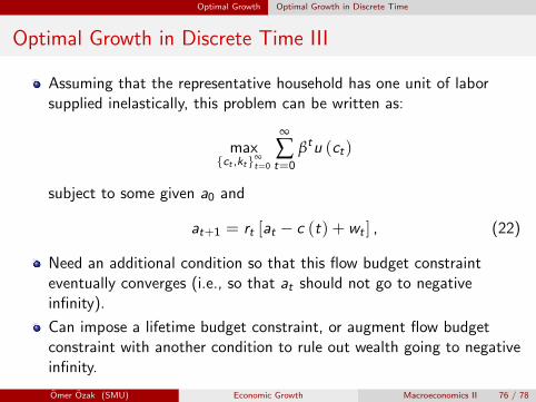
Assuming that the representative household has one unit of laborsupplied inelastically, this problem can be written as:

max{ct ,kt}∞

t=0

∞

∑t=0

βtu (ct)

subject to some given a0 and

at+1 = rt [at − c (t) + wt ] , (22)

Need an additional condition so that this flow budget constrainteventually converges (i.e., so that at should not go to negativeinfinity).

Can impose a lifetime budget constraint, or augment flow budgetconstraint with another condition to rule out wealth going to negativeinfinity.


Optimal Growth Optimal Growth in Continuous Time

Optimal Growth in Continuous Time

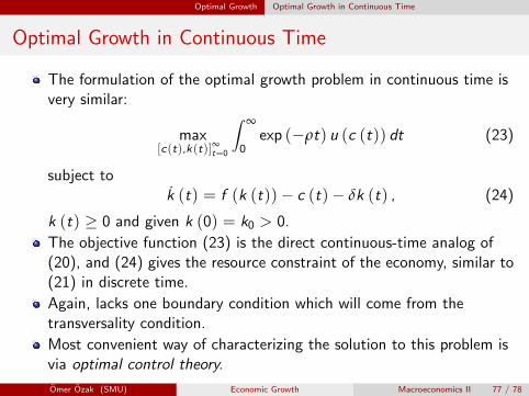
The formulation of the optimal growth problem in continuous time isvery similar:

max[c(t),k(t)]∞t=0

∫ ∞

0exp (−ρt) u (c (t)) dt (23)

subject tok (t) = f (k (t))− c (t)− δk (t) , (24)

k (t) ≥ 0 and given k (0) = k0 > 0.

The objective function (23) is the direct continuous-time analog of(20), and (24) gives the resource constraint of the economy, similar to(21) in discrete time.

Again, lacks one boundary condition which will come from thetransversality condition.

Most convenient way of characterizing the solution to this problem isvia optimal control theory.


Conclusions Conclusions

Conclusions

Models we study in this book are examples of more general dynamicgeneral equilibrium models.

First and the Second Welfare Theorems are essential.

The most general class of dynamic general equilibrium models are notbe tractable enough to derive sharp results about economic growth.

Need simplifying assumptions, the most important one being therepresentative household assumption.


Documents

Foundations of Neoclassical Growth · Foundations of Neoclassical Growth Omer Ozak SMU Macroeconomics II Omer Ozak (SMU) Economic Growth Macroeconomics II 1 / 78. Preliminaries Introduction