Fourier Analysis Methods for PDE’s

R. Danchin

November 14, 2005

2

Contents

1 An introduction to Fourier analysis 71.1 Notations and definitions . . . . . . . . . . . . . . . . . . . . . . . . . . . . . . . 71.2 The Littlewood-Paley decomposition . . . . . . . . . . . . . . . . . . . . . . . . . 8

1.2.1 Bernstein inequalities . . . . . . . . . . . . . . . . . . . . . . . . . . . . . 81.2.2 The nonhomogeneous Littlewood-Paley decomposition . . . . . . . . . . . 91.2.3 About the periodic case . . . . . . . . . . . . . . . . . . . . . . . . . . . . 10

1.3 Littlewood-Paley decomposition and functional spaces . . . . . . . . . . . . . . . 111.3.1 Sobolev and Holder spaces . . . . . . . . . . . . . . . . . . . . . . . . . . . 111.3.2 Besov spaces . . . . . . . . . . . . . . . . . . . . . . . . . . . . . . . . . . 131.3.3 A few properties of Besov spaces . . . . . . . . . . . . . . . . . . . . . . . 15

1.4 Paradifferential calculus . . . . . . . . . . . . . . . . . . . . . . . . . . . . . . . . 211.4.1 Definitions . . . . . . . . . . . . . . . . . . . . . . . . . . . . . . . . . . . 211.4.2 Results of continuity for the paraproduct and the remainder . . . . . . . . 221.4.3 Results of continuity for the product . . . . . . . . . . . . . . . . . . . . 231.4.4 A result of compactness in Besov spaces . . . . . . . . . . . . . . . . . . . 241.4.5 Results of continuity for the composition . . . . . . . . . . . . . . . . . . 27

1.5 Calculus in homogeneous functional spaces . . . . . . . . . . . . . . . . . . . . . 281.5.1 Homogeneous Littlewood-Paley decomposition . . . . . . . . . . . . . . . 291.5.2 Homogeneous Besov spaces . . . . . . . . . . . . . . . . . . . . . . . . . . 291.5.3 Paradifferential calculus in homogeneous spaces . . . . . . . . . . . . . . . 35

1.6 Exercises . . . . . . . . . . . . . . . . . . . . . . . . . . . . . . . . . . . . . . . . 37

2 The heat equation 392.1 Generalities . . . . . . . . . . . . . . . . . . . . . . . . . . . . . . . . . . . . . . . 392.2 A priori estimates in Besov spaces for the heat equation . . . . . . . . . . . . . . 40

2.2.1 Spectral localization . . . . . . . . . . . . . . . . . . . . . . . . . . . . . . 412.2.2 Estimates for the heat equation . . . . . . . . . . . . . . . . . . . . . . . . 422.2.3 A counterexample . . . . . . . . . . . . . . . . . . . . . . . . . . . . . . . 432.2.4 Estimates in nonhomogeneous Besov spaces, and the periodic case . . . . 43

2.3 Optimal well-posedness results for Navier-Stokes equations . . . . . . . . . . . . . 442.3.1 The model . . . . . . . . . . . . . . . . . . . . . . . . . . . . . . . . . . . 442.3.2 About scaling and critical spaces . . . . . . . . . . . . . . . . . . . . . . . 462.3.3 Global well-posedness for small data . . . . . . . . . . . . . . . . . . . . . 472.3.4 Further results . . . . . . . . . . . . . . . . . . . . . . . . . . . . . . . . . 50

2.4 Exercises . . . . . . . . . . . . . . . . . . . . . . . . . . . . . . . . . . . . . . . . 51

3 The transport equation 533.1 Framework and basic properties . . . . . . . . . . . . . . . . . . . . . . . . . . . . 533.2 A priori estimates in Besov spaces . . . . . . . . . . . . . . . . . . . . . . . . . . 543.3 Solving the transport equation in Besov spaces . . . . . . . . . . . . . . . . . . . 58

3

4 CONTENTS

3.4 On the Cauchy problem for a shallow water equation . . . . . . . . . . . . . . . . 603.4.1 About Camassa-Holm equation . . . . . . . . . . . . . . . . . . . . . . . . 603.4.2 A well-posedness result and a blow-up criterion . . . . . . . . . . . . . . . 613.4.3 Uniqueness . . . . . . . . . . . . . . . . . . . . . . . . . . . . . . . . . . . 623.4.4 The proof of existence . . . . . . . . . . . . . . . . . . . . . . . . . . . . . 633.4.5 Blow-up criterion and energy conservation . . . . . . . . . . . . . . . . . . 65

3.5 Exercises . . . . . . . . . . . . . . . . . . . . . . . . . . . . . . . . . . . . . . . . 68

4 A short insight into compressible fluid mechanics 694.1 About the model . . . . . . . . . . . . . . . . . . . . . . . . . . . . . . . . . . . . 69

4.1.1 Physical conservation laws . . . . . . . . . . . . . . . . . . . . . . . . . . . 694.1.2 The full model . . . . . . . . . . . . . . . . . . . . . . . . . . . . . . . . . 704.1.3 Simplifying assumptions . . . . . . . . . . . . . . . . . . . . . . . . . . . . 704.1.4 Barotropic fluids . . . . . . . . . . . . . . . . . . . . . . . . . . . . . . . . 72

4.2 Local well-posedness in critical spaces . . . . . . . . . . . . . . . . . . . . . . . . 724.2.1 The existence proof . . . . . . . . . . . . . . . . . . . . . . . . . . . . . . 73

4.3 Further results . . . . . . . . . . . . . . . . . . . . . . . . . . . . . . . . . . . . . 834.4 Exercises . . . . . . . . . . . . . . . . . . . . . . . . . . . . . . . . . . . . . . . . 84

Bibliographie 87

Introduction

Since the 80’s, Fourier analysis methods have known a growing interest in the study oflinear and nonlinear PDE’s. In particular, techniques based on Littlewood-Paley decompositionand paradifferential calculus have proved to be very efficient. Littlewood-Paley decompositionhas been introduced more than fifty years ago in harmonic analysis but its systematic use inthe PDE’s framework is rather recent. Paradifferential calculus, as for it, has been introducedin 1981 by J.-M. Bony for the study of the propagation of microlocal singularities in nonlinearhyperbolic PDE’s (see [4]).

In the present notes, we aim at giving a survey of those techniques and a few examples ofhow they may used to solve PDE’s. We focus on two linear models: the heat equation andthe transport equation. For each of them, an example of related nonlinear problem is given.Although most of the results we present here belong to the mathematical folklore, we wantto point out that Fourier analysis methods are very efficient to tackle most of well-posednessproblems for evolutionary PDE’s in the whole space or in the torus.

The notes are structured as follows. The first chapter deals with Fourier analysis. Weintroduce Littlewood-Paley decomposition and show how it may used to characterize functionalspaces. We also give a (non so) short insight into the theory of homogeneous spaces whichturn out to be well adapted to the study of many PDE’s and are omitted in most of textbookson functional analysis. Finally, we introduce some smatterings of paradifferential calculus andprove estimates for the product of two temperate distributions, when it makes sense.

In the second chapter, we focus on the heat equation. We state a priori estimates in Besovspaces with optimal gain of derivatives. As an application, we prove global well-posedness inBesov spaces with critical regularity for the incompressible Navier-Stokes equations with smalldata.

The third chapter is devoted to the study of transport equations associated to Lipschitzvectorfields. We state a priori estimates in Besov spaces then apply our results to the study ofa shallow water equation.

In the last chapter, we give an example of coupling between heat equation and transportequation, namely the compressible barotropic Navier-Stokes system. Well-posedness in Besovspaces with critical regularity is stated.

Acknowledgments The author is grateful to J.-Y. Chemin for supplying most material forthe first chapter, to Zhouping Xin, Chiaojang Xu and Yinbin Deng for the invitation to deliverthis course at Wuhan Normal University, to Ping Zhang for his kind invitation at the ChineseAcademy of Sciences in Beijing and to Yuxin Ge for helping me to communicate between Franceand China.

5

6 CONTENTS

Chapter 1

An introduction to Fourier analysis

1.1 Notations and definitions

• S stands for the Schwartz space of smooth functions over RN whose derivatives of all orderdecay at infinity. The space S is endowed with the topology generated by the followingfamily of semi-norms:

‖u‖M,S := supx∈RN

|α|≤M

(1 + |x|)M |∂αu(x)| for all u ∈ S and M ∈ N.

• The set S ′ of temperate distributions is the dual set of S for the usual pairing.

• For any u ∈ S, the Fourier transform of u denoted by u or Fu is defined by

∀ξ ∈ RN , u(ξ) = Fu(ξ) :=∫

RN

e−iξ·xu(x) dx.

The Fourier transform maps S into and onto itself, and the inverse Fourier transform isgiven by the formula F−1 = (2π)−NF .

• The Fourier transform is extended by duality to the whole S ′ by setting

< u, ϕ >:=< u, ϕ >S′,S

whenever u ∈ S ′ and ϕ ∈ S.

• Derivatives: for all multi-index α ∈ NN , we have

F(∂αxu) = (iξ)αFu and F(xαu) = (−i)|α|∂α

ξ Fu.

• Algebraic properties: for (u, v) ∈ S × S ′ , we have u ∗ v ∈ S ′ and

F(u ∗ v) = FuFv.

The above formula also holds true for couples of distributions with compact supports.

• Multipliers: if A is a smooth function with polynomial growth at infinity, and u ∈ S ′(RN )then we set A(D)u := F−1

(AFu

).

• The open (resp. closed) ball with radius R centered at x0 ∈ RN is denoted by B(0, R)(resp. B(0, R)).

• The shell ξ ∈ RN |R1 ≤ |ξ| ≤ R2 is denoted by C(0, R1, R2).

• The notation A . B means that A ≤ CB for some “irrelevant” constant C (which maychange from line to line but whose meaning is clear from the context). Likewise, A ≈ Bmeans that A . B and B . A.

7

8 CHAPTER 1. AN INTRODUCTION TO FOURIER ANALYSIS

1.2 The Littlewood-Paley decomposition

1.2.1 Bernstein inequalities

As recalled in the previous section, in Fourier variables differentiating with respect to xj amountsto multiplying by the function ξ 7→ iξj .

As far as one is concerned with estimates in Lebesgue spaces and whenever the distributionwe consider is well localized in Fourier variables, Bernstein lemma states that differentiatingamounts to multiplying by an appropriate constant

Lemma (Bernstein). Let k be in N. Let (R1, R2) satisfy 0 < R1 < R2. There exists a constantC depending only on r1, r2, N, such that for all 1 ≤ a ≤ b ≤ ∞ and u ∈ La, we have

Supp u ⊂ B(0, R1λ) ⇒ sup|α|=k ‖∂αu‖Lb ≤ Ck+1λk+N( 1a− 1

b) ‖u‖La ,(1.1)

Supp u ⊂ C(0, R1λ,R2λ) ⇒ C−k−1λk ‖u‖La ≤ sup|α|=k ‖∂αu‖La ≤ Ck+1λk ‖u‖La .(1.2)

Proof: Arguing by rescaling, one can assume with no loss of generality that λ = 1.

Now, fix a smooth function φ compactly supported and such that φ ≡ 1 in a neighborhoodof the ball B(0, R1). We notice that u = φu. Hence, denoting g := F−1φ, we get for allmulti-index α,

∂αu(x) =∫∂αg(y)u(x− y)dy.

Taking advantage of Young inequality, we thus get

‖∂αu‖Lb ≤ ‖∂αg‖Lc ‖u‖La with1c

= 1 +1b− 1a·

Because‖∂αg‖Lc ≤ ‖∂αg‖L∞ + ‖∂αg‖L1 ≤ Ck+1,

the proof of the first inequality is complete.

For proving (1.2), we first notice that the inequality on the right is a particular case of(1.1). Next, we introduce a smooth function ϕ with compact support in RN \ 0 andsuch that ϕ ≡ 1 in a neighborhood of the shell C(0, R1, R2).

As∑

|α|=k(iξ)α(−iξ)α = |ξ|2k, we have

(1.3) u =∑|α|=k

gα ? ∂αu with gα(ξ) := (iξ)α|ξ|−2kϕ(ξ).

Making use of Young inequality, one can now conclude to the left inequality in (1.2).

Remark. In other words, if u is supported in a ball of radius λ then differentiating once is notworse that multiplying by λ. If u is supported in the shell ξ ∈ RN |R1λ ≤ |ξ| ≤ R2λ then,up to an irrelevant constant, differentiating once amounts to multiplying by λ.

In most applications, the functions we deal with are not spectrally supported in a shell orin a ball. Hence, if one wants to take advantage of the nice properties exhibited in Bernsteinlemma, one first has to split the function into pieces which are spectrally supported in a shellor in a ball. This may be done by introducing a dyadic partition of unity in Fourier variables.There are two main ways to proceed. Either the decomposition is made indistinctly over thewhole space RN (and we say that the decomposition is homogeneous), or the low frequenciesare treated separately (and the decomposition is said to be nonhomogeneous).

Both decompositions have advantages and drawbacks. The nonhomogeneous one is moresuitable for characterizing the usual functional spaces whereas the properties of invariance bydilation of the homogeneous decomposition may be more adapted for studying certain PDE’s orstating optimal functional inequalities having some scaling invariance.

1.2. THE LITTLEWOOD-PALEY DECOMPOSITION 9

1.2.2 The nonhomogeneous Littlewood-Paley decomposition

Let α > 1 and (ϕ, χ) be a couple of smooth functions valued in [0, 1], such that ϕ is supportedin the shell ξ ∈ RN |α−1 ≤ |ξ| ≤ 2α, χ is supported in the ball ξ ∈ RN | |ξ| ≤ α and

∀ξ ∈ RN , χ(ξ) +∑q∈N

ϕ(2−qξ) = 1.

For u ∈ S ′, one can define nonhomogeneous dyadic blocks as follows. Let

∆qu := 0 if q ≤ −2,

∆−1u := χ(D)u = h ? u with h := F−1χ,

∆qu := ϕ(2−qD)u = 2qN

∫h(2qy)u(x− y)dy with h = F−1ϕ, if q ≥ 0.

One can prove that we haveu =

∑q∈Z

∆qu in S ′(RN )

for all temperate distribution u (see exercise 1.2). The right-hand side is called nonhomogeneousLittlewood-Paley decomposition of u.

It is also convenient to introduce the following low frequency cut-off:

Squ :=∑

p≤q−1

∆pu.

Of course, S0u = ∆−1u. Because ϕ(ξ) = χ(ξ/2) − χ(ξ) for all ξ ∈ RN , one can prove that,more generally, we have

Squ = χ(2−qD)u =∫h(2qy)u(x− y)dy for all q ∈ N.

The Littlewood-Paley decomposition is “almost” orthogonal in L2. Assuming for instance thatα = 4/3, we have the following result1:

Proposition 1.2.1. For any u ∈ S ′(RN ) and v ∈ S ′(RN ), the following properties hold:

∆p∆qu ≡ 0 if |p− q| ≥ 2,∆q(Sp−1u∆pv) ≡ 0 if |p− q| ≥ 5.

Remark. At this point, one can wonder why it is so important to choose smooth cut-off functionsχ and ϕ for defining a Littlewood-Paley decomposition. Obviously, setting ∆′

−1u := 1|ξ|≤1(D)uand ∆′

qu := 12q≤|ξ|≤2q+1(D)u would define a dyadic spectral decomposition which, in addition,would be orthogonal in L2.

In most applications however, it is crucial that we have

‖∆qu‖Lp ≤ C ‖u‖Lp

for some constant C independent of q.Alas, unless p = 2, the above inequality fails to be true with ∆′

qu instead of ∆qu (seeexercise 1.5).

1Of course, similar properties may be proved for any α > 1.

10 CHAPTER 1. AN INTRODUCTION TO FOURIER ANALYSIS

1.2.3 About the periodic case

Throughout, a1, · · · , aN denote N positive reals. We denote by TNa the periodic box with

period 2πai in the i-th direction, and QNa := (0, 2πa1) × · · · × (0, 2πaN ). We also introduce

ZNa := Z/a1 × · · · × Z/aN the dual lattice associated to TN

a .We claim that the analysis of the previous section for temperate distributions defined on the

whole space RN may be carried out to S ′(TNa ) with very few changes.

Indeed, decompose u ∈ S ′(TNa ) into Fourier series:

u(x) =∑

β∈eZNa

uβeiβ·x with uβ :=

1|TN

a |

∫TN

a

e−iβ·yu(y) dy.

Denotinghq(x) =

∑β∈eZN

a

ϕ(2−qβ)eiβ·x,

one can now define the periodic dyadic blocks as follows:

∆perq u(x) :=

∑β∈eZN

a

ϕ(2−qβ)uβ eiβ·x =

1|TN

a |

∫TN

a

hq(y)u(x− y) dy for all q ∈ Z

and the low frequency cut-off:

Sperq u(x) := u0 +

∑p≤q−1

∆perp u(x) =

∑β∈eZN

a

χ(2−qβ)uβeiβ·x.

It is obvious that ∆perp u = 0 for negative enough p (depending on a) and that

u = u0 +∑

q

∆perq u in S ′(TN

a ).

Now, to any temperate distribution u over RN , one can associate the periodic distribution uper

defined by

uper(x) :=∑

α∈ZN2πa

u(x+ α) where ZN2πa := 2πa1Z× · · · × 2πaNZ.

For uper, both periodic and nonhomogeneous Littlewood-Paley decompositions are available. Itturns out that periodic blocks and nonhomogeneous blocks coincide in the following sense:

Proposition 1.2.2. For all temperate distribution u over RN , one has

∀q ∈ Z,(ϕ(2−qD)u

)per = ∆perq uper.

Proof: This is actually an easy consequence of the following Poisson formula for θ ∈ S ′(RN ):

1(2π)N

∑β∈ZN

θ(β) =∑

α∈ZN

θ(2πα),

which, after a change of variables yields

(1.4) ∀u ∈ S ′(RN ), ∀x ∈ RN ,1

|TNa |

∑β∈eZN

a

eiβ·xu(β) =∑

α∈ZN2πa

u(x+ α).

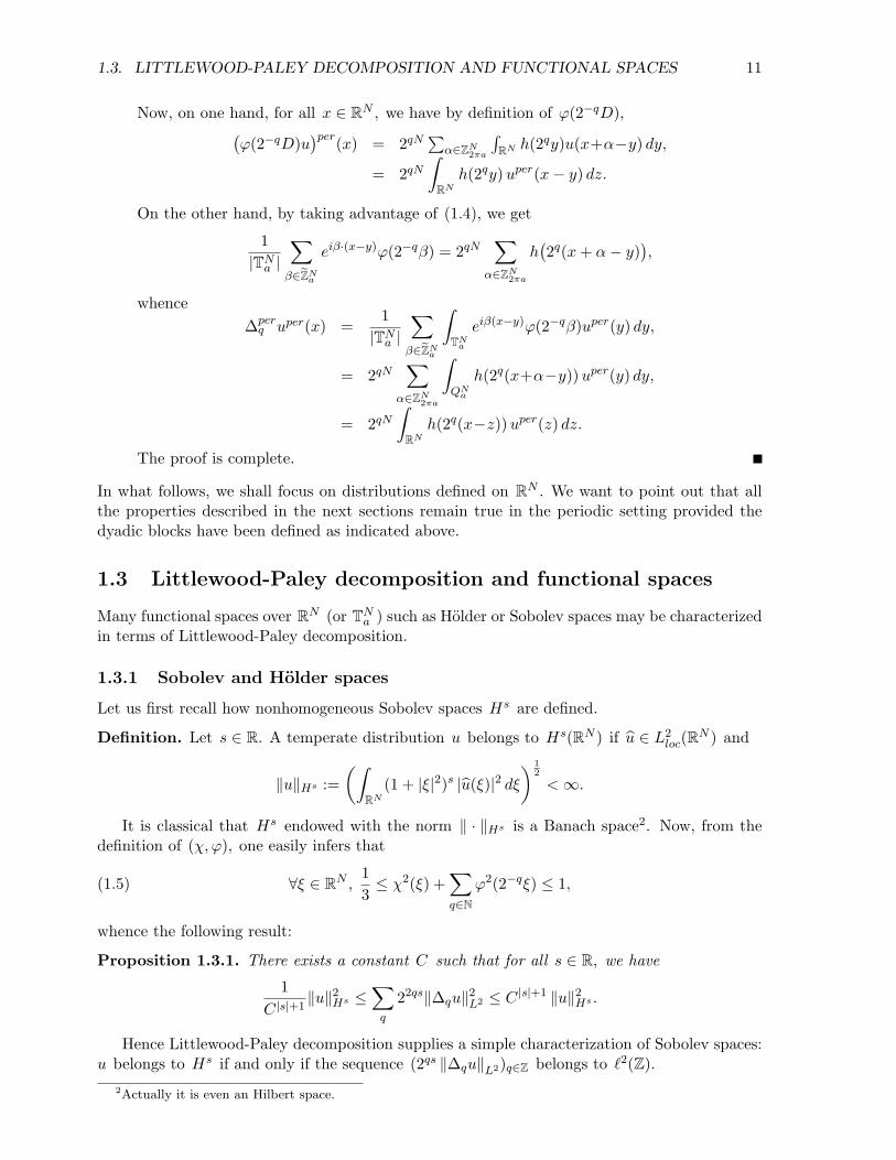
1.3. LITTLEWOOD-PALEY DECOMPOSITION AND FUNCTIONAL SPACES 11

Now, on one hand, for all x ∈ RN , we have by definition of ϕ(2−qD),(ϕ(2−qD)u

)per(x) = 2qN∑

α∈ZN2πa

∫RN h(2qy)u(x+α−y) dy,

= 2qN

∫RN

h(2qy)uper(x− y) dz.

On the other hand, by taking advantage of (1.4), we get

1|TN

a |∑

β∈eZNa

eiβ·(x−y)ϕ(2−qβ) = 2qN∑

α∈ZN2πa

h(2q(x+ α− y)

),

whence∆per

q uper(x) =1

|TNa |

∑β∈eZN

a

∫TN

a

eiβ(x−y)ϕ(2−qβ)uper(y) dy,

= 2qN∑

α∈ZN2πa

∫QN

a

h(2q(x+α−y))uper(y) dy,

= 2qN

∫RN

h(2q(x−z))uper(z) dz.

The proof is complete.

In what follows, we shall focus on distributions defined on RN . We want to point out that allthe properties described in the next sections remain true in the periodic setting provided thedyadic blocks have been defined as indicated above.

1.3 Littlewood-Paley decomposition and functional spaces

Many functional spaces over RN (or TNa ) such as Holder or Sobolev spaces may be characterized

in terms of Littlewood-Paley decomposition.

1.3.1 Sobolev and Holder spaces

Let us first recall how nonhomogeneous Sobolev spaces Hs are defined.

Definition. Let s ∈ R. A temperate distribution u belongs to Hs(RN ) if u ∈ L2loc(RN ) and

‖u‖Hs :=(∫

RN

(1 + |ξ|2)s |u(ξ)|2 dξ) 1

2

<∞.

It is classical that Hs endowed with the norm ‖ · ‖Hs is a Banach space2. Now, from thedefinition of (χ, ϕ), one easily infers that

(1.5) ∀ξ ∈ RN ,13≤ χ2(ξ) +

∑q∈N

ϕ2(2−qξ) ≤ 1,

whence the following result:

Proposition 1.3.1. There exists a constant C such that for all s ∈ R, we have

1C |s|+1

‖u‖2Hs ≤

∑q

22qs‖∆qu‖2L2 ≤ C |s|+1 ‖u‖2

Hs .

Hence Littlewood-Paley decomposition supplies a simple characterization of Sobolev spaces:u belongs to Hs if and only if the sequence (2qs ‖∆qu‖L2)q∈Z belongs to `2(Z).

2Actually it is even an Hilbert space.

12 CHAPTER 1. AN INTRODUCTION TO FOURIER ANALYSIS

Let us now focus on Holder spaces.

Definition. Let r ∈ (0, 1). We denote by Cr the set of bounded functions u : RN → R suchthat there exists C ≥ 0 with

(1.6) ∀(x, y) ∈ RN × RN , |u(x)− u(y)| ≤ C|x− y|r.

More generally, if r > 0 is not an integer, we denote by Cr the set of [r] times3 differentiablefunctions u such that ∂αu ∈ Cr−[r] for all |α| ≤ r.

One can easily prove that the set Cr endowed with the norm

‖u‖Cr :=∑|α|≤[r]

(‖∂αu‖L∞ + sup

x 6=y

|∂αu(x)− ∂αu(y)||x− y|r−[r]

)

is a Banach space.In the case r ∈ R+ \ N, the Littlewood-Paley decomposition supplies a very simple charac-

terization of Cr :

Proposition 1.3.2. There exists a constant C such that for all r ∈ R+ \ N and u ∈ Cr wehave

supq

2qr ‖∆qu‖L∞ ≤ Cr+1

[r]!‖u‖Cr .

Conversely, if the sequence (2qr ‖∆qu‖L∞)q≥−1 is bounded then

‖u‖Cr ≤ Cr+1

(1

r − [r]+

1[r] + 1− r

)sup

q2qr ‖∆qu‖L∞ .

Proof: Let us just sketch the proof (for more details see [10]).

Let us first notice that, owing to∫xαh(x)dx = 0 for all multi-index α, one can write

(1.7) ∀q ∈ N, ∆qu(x) = 2qN

∫h(2q(x− y))

(u(y)−

[r]∑k=1

1k!Dku(x)(y − x)(k)

)dy.

Applying the [r]-th order Taylor formula for bounding the right-hand side of (1.7) andusing the fact that ‖∆−1u‖L∞ ≤ C ‖u‖L∞ yields the first inequality.

For proving the converse inequality, we notice that since for all multi-index we have ∂αu =∑q ∂

α∆qu, Bernstein lemma insures that

‖∂αu‖L∞ ≤ C1+r

r − [r]sup

q2qr ‖∆qu‖L∞

whenever |α| ≤ [r].

Next, for all multi-index α of size [r], all (x, y) ∈ RN ×RN such that |x− y| ≤ 1 and allQ ∈ N, we have

|∂αu(x)− ∂αu(y)| ≤Q−1∑q=−1

|∂α∆qu(x)− ∂α∆qu(y)|++∞∑q=Q

|∂α∆qu(x)− ∂α∆qu(y)|.

3From now on, the notation [r] stands for the integer part of r.

1.3. LITTLEWOOD-PALEY DECOMPOSITION AND FUNCTIONAL SPACES 13

Making use of Bernstein lemma, we end up with

|∂αu(x)− ∂αu(y)| ≤ Cr+1(supq≥0

2qr ‖∆qu‖L∞

)( Q∑q=−1

2−q(r−[r]−1)|x− y|+∑

q≥Q+1

2−q(r−[r])).

Choosing Q = [− log2 |x− y|] + 1 yields the wanted inequality.

Remark. The above characterization of Holder spaces is false if r is an integer (see exercise 1.9).

1.3.2 Besov spaces

From now on, we make the convention that for all non-negative sequence (aq)q∈Z, the notation(∑q a

rq

) 1r stands for supq aq in the case r = ∞.

The characterizations of Sobolev and Holder spaces given in the previous part naturally leadto the following definition:

Definition. Let 1 ≤ p, r ≤ ∞ and s ∈ R. For u ∈ S ′(RN ), we set

‖u‖Bsp,r

:=(∑

q

(2qs ‖∆qu‖Lp

)r) 1r

.

The Besov space Bsp,r is the set of temperate distributions u such that ‖u‖Bs

p,r<∞.

Before going further into the study of Besov spaces, let us state two important lemmas. Thefirst one reads:

Lemma 1.3.3. Let (uq)q∈N be a sequence of bounded functions such that the Fourier transformof uq is supported in dyadic shells. Let us assume that, for some M ≥ 0, we have

‖uq‖L∞ ≤ C2qM .

Then the series∑

q uq is convergent in S ′.

Proof: After rescaling, relation (1.3) rewrites

(1.8) uq = 2−qk∑|α|=k

2qNgα(2q·) ? ∂αuq.

Therefore, for any test function φ in S, we have

(1.9) 〈uq, φ〉 = (−1)k2−qk∑|α|=k

〈uq, 2qN gα(2q·) ? ∂αφ〉 with g(z) = g(−z).

Hence|〈uq, φ〉| ≤ C2−qk

∑|α|=k

2qM‖∂αφ‖L1 .

Let us choose k > M . Then∑

q〈uq, φ〉 is a convergent series, the sum of which is lessthan C‖φ‖P,S for some large enough integer P. Thus the formula

〈u, φ〉 := limq→∞

∑q′≤q

〈∆q′u, φ〉

defines a temperate distribution.

14 CHAPTER 1. AN INTRODUCTION TO FOURIER ANALYSIS

The second important lemma is the following one:

Lemma 1.3.4. Let s ∈ R and 1 ≤ p, r ≤ ∞. Let (uq)q≥−1 be a sequence of functions such that(∑q≥−1

(2qs ‖uq‖Lp

)r) 1r

<∞.

(i) If Supp u−1 ⊂ B(0, R2) and Supp uq ⊂ C(0, 2qR1, 2qR2) for some 0 < R1 < R2 thenu :=

∑q≥−1 uq belongs to Bs

p,r and there exists a universal constant C such that

‖u‖Bsp,r≤ C1+|s|

(∑q≥−1

(2qs ‖uq‖Lp

)r) 1r

.

(ii) If s is positive and Supp uq ⊂ B(0, 2qR) for some R > 0 then u :=∑

q≥−1 uq belongs toBs

p,r and there exists a universal constant C such that

‖u‖Bsp,r≤ C1+s

s

(∑q≥−1

(2qs ‖uq‖Lp

)r) 1r

.

Proof: Under the hypothesis of the first assertion and according to Bernstein lemma, we have

‖uq‖L∞ ≤ C2q“

Np−s

”. Lemma 1.3.3 thus implies that

∑q uq is a convergent series in S ′ .

Next, we notice that there exists an integer N0 so that

|q′ − q| ≥ N0 =⇒ ∆q′uq = 0.

Therefore, with the convention that uq = 0 if q ≤ −2, we can write that

‖∆q′u‖Lp = ‖∑

|q−q′|<N0

∆q′uq‖Lp

≤ C∑

|q−q′|<N0

‖uq‖Lp .

So, we obtain that

2q′s‖∆q′u‖Lp ≤ C∑

|q−q′|≤N0

2q′s‖uq‖Lp

≤ C1+|s|∑

|q−q′|≤N0

2qs‖uq‖Lp ,

and we deduce from convolution inequalities that

‖u‖Bsp,r≤ C1+|s|

(∑q∈N

2rqs‖uq‖rLp

) 1r

,

which is exactly the first result.

For proving the second result, we first notice that for any q, we have

‖uq‖Lp ≤ C2−qs.

1.3. LITTLEWOOD-PALEY DECOMPOSITION AND FUNCTIONAL SPACES 15

As s is positive, this implies that∑

q uq is a convergent series in Lp . Next, we notice thatthere exists some N1 ∈ N such that

q′ ≥ q +N1 =⇒ ∆q′uq = 0.

Now, we write that

‖∆q′u‖Lp =∥∥∥∥ ∑

q>q′−N1

∆q′uq

∥∥∥∥Lp

,

≤ C∑

q>q′−N1

‖uq‖Lp .

So, we get that2q′s‖∆q′u‖Lp ≤ C

∑q≥q′−N1

2(q′−q)s2qs‖uq‖Lp .

In other words, we have

2q′s‖∆q′u‖Lp ≤ C(ck) ? (d`) with ck = 1[−N1,+∞[(k)2−ks and d` = 2`s‖u`‖Lp .

Applying convolution inequalities for series completes the proof of the second property.

Corollary. The definition of the space Bsp,r does not depend on the choice of the couple (χ, ϕ)

defining the Littlewood-Paley decomposition.

Remark. The Besov spaces have been obtained by taking first the Lp norm on each dyadicblock, then taking a weighted `r norm. It turns out that taking first the weighted `r normand next the Lp norm over RN is also relevant. This yields new Banach spaces called Triebel-Lizorkin spaces and denoted by F s

p,r. Using such spaces may be appropriate for studying certainproblems. In particular, if 1 < p < ∞, the space F 0

p,2 coincides with the Lebesgue space Lp

and, more generally, F sp,2 coincide with the potential space Hs

p of temperate distributions u

such that (I −∆)s2 belongs to Lp.

The reader is referred to [36] or [38] for a more complete study of Triebel-Lizorkin spaces.

1.3.3 A few properties of Besov spaces

In the following proposition, we give a first list of important properties of Besov spaces.

Proposition 1.3.5. Let s ∈ R and 1 ≤ p, r ≤ ∞.

(i) Topological properties: Bsp,r is a Banach space which is continuously embedded in S ′.

(ii) Density: the space C∞c of smooth functions with compact support is dense in Bsp,r if and

only if p and r are finite.

(iii) Duality: for all s ∈ R and 1 ≤ p, r <∞, the space B−sp′,r′ is the dual space of Bs

p,r.

If 1 ≤ p <∞, the completion Bsp,∞ of C∞c for the norm ‖ · ‖Bs

p,∞ is the predual of B−sp′,1.

(iv) Separability: If 1 ≤ p, r <∞ then the space Bsp,r is separable. The same holds for Bs

p,∞.

(v) Embeddings: we have

(a) Bsp,r → Bes

p,er whenever s < s or s = s and r ≥ r,

(b) Bsp,r → B

s−N( 1p− 1ep )ep,r whenever p ≥ p,

16 CHAPTER 1. AN INTRODUCTION TO FOURIER ANALYSIS

(c) we have B0∞,1 → C ∩L∞. If p <∞ then the space B

Np

p,1 is continuously embedded inthe space C0 of continuous bounded functions which decay at infinity.

(vi) Fatou property: if (un)n∈N is a bounded sequence of Bsp,r which tends to u in S ′ then

u ∈ Bsp,r and

‖u‖Bsp,r≤ lim inf ‖un‖Bs

p,r.

(vii) Complex interpolation: if u ∈ Bsp,r ∩Bes

p,r and θ ∈ [0, 1] then u ∈ Bθs+(1−θ)esp,r and

‖u‖B

θs+(1−θ)esp,r

≤ ‖u‖θBs

p,r‖u‖1−θ

Besp,r.

(viii) Real interpolation: if u ∈ Bsp,∞ ∩ Bes

p,∞ and s < s then u belongs to Bθs+(1−θ)esp,1 for all

θ ∈ (0, 1) and there exists a universal constant C such that

‖u‖B

θs+(1−θ)esp,1

≤ C

θ(1−θ)(s−s)‖u‖θ

Bsp,∞‖u‖1−θ

Besp,∞

.

Proof: Let us first prove that Bsp,r is continuously embedded in S ′. By definition, Bs

p,r is asubspace of S ′ . Thus it suffices to prove that there exist a constant C and an integer Msuch that for any φ ∈ S we have

(1.10) |〈u, φ〉| ≤ C‖u‖Bsp,r‖φ‖M,S .

Taking advantage of (1.9) with ∆qu instead of uq, we see that for all k ∈ N, there existsan integer Mk and a constant Ck such that

|〈∆qu, φ〉| ≤ Ck2−q(2q(1−k) ‖∆qu‖L∞

)‖φ‖Mk,S .

According to Bernstein lemma, we have ‖∆qu‖L∞ ≤ C2q Np ‖∆qu‖Lp . Hence, if k has been

chosen so large as to satisfy s−N/p ≥ 1− k, we have

|〈∆qu, φ〉| ≤ Ck2−q‖u‖Bsp,r‖φ‖Mk,S

which, after summation on q, yields inequality(1.10).

Next, consider (u(n))n∈N a Cauchy sequence in Bsp,r . Inequality (1.10) implies that for

any test function φ in S , sequence (〈u(n), φ〉)n∈N is a Cauchy sequence in R. Thus theformula

〈u, φ〉 := limn→∞

〈u(n), φ〉

defines a temperate distribution. By definition of the norm of Bsp,r, sequence (∆qu

(n))n∈Nis a Cauchy sequence in Lp for any q . Thus an element uq of Lp exists such that(∆qu

(n))n∈N converges to uq in Lp . As the sequence (u(n))n∈N converges to u in S ′ weactually have ∆qu = uq.

Fix a Q ∈ N and a positive ε. Since for all q ≥ −1, ∆qu(n) tends to ∆qu in Lp, we have

for all n ∈ N,(∑q≤Q

(2qs‖∆q(u(n) − u)‖Lp

)r) 1r

= limm→∞

(∑q≤Q

(2qs‖∆q(u(n) − u(m))‖Lp

)r) 1r

.

1.3. LITTLEWOOD-PALEY DECOMPOSITION AND FUNCTIONAL SPACES 17

Because the argument of the limit in the right-hand side is bounded by ‖u(n) − u(m)‖Bsp,r

and (u(n))n∈N is a Cauchy sequence in Bsp,r, one can now conclude that there exists a n0

(independent of Q) such that for all n ≥ n0, we have

(∑q≤Q

(2qs‖∆q(u(n) − u)‖Lp

)r) 1r

≤ ε.

Letting Q go to infinity insures that (u(n))n∈N tends to u in Bsp,r.

Let us tackle the proof of (ii). Consider first the case where r is finite. Let u be in Bsp,r

and ε > 0. Since r is finite, there exists an integer q such that

(1.11) ‖u− Squ‖Bsp,r<ε

2·

Now let φ be in C∞c . For any q′ ∈ N, Bernstein lemma insures that we have,

2q′s‖∆q′(φSqu− Squ)‖Lp ≤ 2−q′2q′([s]+2)‖∆q′(φSqu− Squ)‖Lp

≤ Cs2−q′ sup|α|=[s]+2

‖∂α(φSqu− Squ)‖Lp .

From the above inequality, we get that

(1.12) ‖φSqu− Squ‖Bsp,r≤ Cs

(‖(1− φ)Squ‖Lp + sup

|α|=[s]+2‖∂α((1−φ)Squ)‖Lp

).

Let us consider a sequence (φn)n∈N such that all the derivatives of φn of order less thanor equal to [s] + 2 are uniformly bounded with respect to n and such that φn ≡ 1 in aneighborhood of the ball B(0, n). If p is finite, combining Leibniz formula and Lebesguetheorem, we discover that

limn→∞

‖(1−φn)Squ‖Lp + sup|α|=[s]+2

‖∂α((1−φn)Squ)‖Lp = 0·

Thus a function φ in C∞c exists such that

Cs

(‖(1− φ)Squ‖Lp + sup

|α|=[s]+2‖∂α((1−φ)Squ)‖Lp

)<ε

2· .

Combining (1.11) and (1.12), we end up with

‖φSqu− u‖Bsp,r< ε.

As Squ is a smooth function, this completes the proof in the case p, r <∞.

Now, it is obvious that the set C∞b of smooth functions with bounded derivatives at allorders is embedded in any space Bs

∞,r. Therefore C∞c cannot be a dense subset of Bs∞,r.

Finally, the closure of C∞c for the Besov norm Bsp,∞ is the space of temperate distributions

u such thatlim

q→∞2qs‖∆qu‖Lp = 0,

which is a strict subspace of Bsp,∞. This completes the proof of (ii).

18 CHAPTER 1. AN INTRODUCTION TO FOURIER ANALYSIS

In order to prove the properties of duality, we use the fact that the map

u 7−→ (∆qu)q≥−1

is a (bi)continuous isomorphism between Bsp,r and4 `rs(L

p).

Assume that 1 ≤ p < ∞. On one hand, if in addition 1 ≤ r < ∞, it is obvious that`r′−s(L

p′) is the dual of `rs(Lp). On the other hand, `1−s(L

p′) is the dual space of the set ofLp valued sequences (zq)q≥−1 such that

limq→+∞

2qs ‖zq‖Lp = 0.

Now, one can prove that Bsp,∞ is the space of temperate distributions u such that

limq→+∞

2qs ‖∆qu‖Lp = 0,

whence the desired result.

The proof of (iv) also relies on the use of the map u 7−→ (∆qu)q≥−1. The details are leftto the reader.

Let us now prove (v). Considering that `r(Z) ⊂ `er(Z) for r ≤ r, the first embedding isstraightforward. In order to prove the second embedding, we apply Bernstein lemma andget

‖S0u‖Lep ≤ C‖S0u‖Lp and ‖∆qu‖Lep ≤ C2qN“

1p− 1ep

”‖∆qu‖Lp if q ∈ N,

whence the result.

For proving that BNp

p,1 → Cb we use again Bernstein lemma and get that

‖∆qu‖L∞ ≤ 2q Np ‖∆qu‖Lp .

This insures that the series∑

∆qu of continuous bounded functions converges uniformly onRN . Hence u is a bounded continuous function. Besides, it is obvious that the embedding

is continuous. If p is finite, one can use in addition that C∞c is dense in BNp

p,1 and concludethat u decays at infinity.

Let us now focus on the proof of (vi). Let (un)n∈N be a bounded sequence of Bsp,r which

tends to some u in S ′. This insures that for all q ∈ Z, sequence (∆qun)n∈N tends to ∆quin S ′. Since (∆qun)n∈N is a bounded sequence in Lp ∩ C∞b , one can conclude that ∆qubelongs to Lp ∩ C∞b and that

‖∆qu‖Lp ≤ lim inf ‖∆qun‖Lp .

Now, for all Q ∈ N, we have(∑Qq=−1

(2qs ‖∆qu‖Lp

)r) 1r

≤(∑Q

q=−1

(2qs lim inf ‖∆qun‖Lp

)r) 1r

,

≤ lim inf(∑Q

q=−1

(2qs ‖∆qun‖Lp

)r) 1r

,

≤ lim inf ‖un‖Bsp,r.

Letting Q go to infinity completes the proof of (vi).4Here `rs stands for the set of sequences (zq)q≥−1 such that ‖(2qszq)‖`r <∞.

1.3. LITTLEWOOD-PALEY DECOMPOSITION AND FUNCTIONAL SPACES 19

Property (vii) is a straightforward consequence of Holder inequality.

For proving (viii), we write

‖u‖B

θs+(1−θ)esp,1

=∑q≤Q

2q(θs+(1−θ)es)‖∆qu‖Lp +∑q>Q

2q(θs+(1−θ)es)‖∆qu‖Lp

for some Q to be chosen hereafter.

Now, by definition of the Besov norms, we have

2q(θs+(1−θ)es)‖∆qu‖Lp ≤ 2q(1−θ)(es−s)‖u‖Bsp,∞ ,

2q(θs+(1−θ)es)‖∆qu‖Lp ≤ 2−qθ(es−s)‖u‖Besp,∞

.

Thus we infer that

‖u‖B

θs+(1−θ)esp,1

≤ ‖u‖Bsp,∞

∑q≤Q

2q(1−θ)(es−s) + ‖u‖Besp,∞

∑q>Q

2−qθ(es−s)

≤ ‖u‖Bsp,∞

2(Q+1)(1−θ)(es−s)

2(1−θ)(es−s) − 1+ ‖u‖Bes

p,∞

2−Qθ(es−s)

1− 2−θ(es−s)·

In order to complete the proof of (viii), it suffices to choose Q such that

‖u‖Besp,∞

‖u‖Bsp,∞

≤ 2Q(es−s) < 2‖u‖Bes

p,∞

‖u‖Bsp,∞

.

One can wonder how far is Bsp,∞ from Bs

p,1, or in other words, what happens if one lets θ tendsto 1 in proposition 1.3.5.(viii). Of course, one already knows that

Bsp,1 → Bs

p,r → Bsp,∞.

A more precise answer is given by the following logarithmic interpolation result:

Proposition 1.3.6. There exists a constant C such that for all s ∈ R, ε > 0 and 1 ≤ p ≤ ∞,we have

‖u‖Bsp,1≤ C

1+εε

‖u‖Bsp,∞

(1 + log

‖u‖Bs+εp,∞

‖u‖Bsp,∞

).

Proof: Let Q be a positive integer to be fixed hereafter. We have

‖u‖Bsp,1

=∑q<Q

2qs‖∆qu‖Lp +∑q≥Q

2qs‖∆qu‖Lp ,

whence,

‖u‖Bsp,1≤ (Q+ 1)‖u‖Bs

p,∞ +2−Qε

1− 2−ε‖u‖Bs+ε

p,∞.

Choosing for Q the closest positive integer to1ε

log2

‖u‖Bs+εp,∞

‖u‖Bsp,∞

yields the result.

We now want to study how multipliers operate on Besov spaces. Before stating our result, weneed to define the multipliers we are going to consider.

20 CHAPTER 1. AN INTRODUCTION TO FOURIER ANALYSIS

Definition. A smooth function f : RN → R is said to be a Sm -multiplier if for all multi-indexα, there exists a constant Cα such that

∀ξ ∈ RN , |∂αf(ξ)| ≤ Cα(1 + |ξ|)m−|α|.

Proposition 1.3.7. Let m ∈ R and f be a Sm -multiplier. Then for all s ∈ R and 1 ≤ p, r ≤ ∞the operator f(D) is continuous from Bs

p,r to Bs−mp,r .

Proof: Let ϕ be a smooth function supported in a shell and such that ϕ ≡ 1 on Supp ϕ. Itis clear that we have

∆qf(D)u = ϕ(2−qD)f(D) ∆qu for all q ∈ N.

Hence, by virtue of convolution inequalities, we have

‖∆qf(D)u‖Lp ≤ ‖kq‖L1 ‖∆qu‖Lp

withkq(x) :=

1(2π)N

∫eix·ξf(ξ)ϕ(2−qξ) dξ.

By performing an easy change of variables, we notice that ‖kq‖L1 = ‖`q‖L1 with

`q(y) :=1

(2π)N

∫eiy·ηϕ(η)f(2qη) dη.

Now, for all M ∈ N, we have

(1 + |y|2)M`q(y) =∫

(1−∆η)M(eiy·η

)ϕ(η)f(2qη) dη,

=∫eiy·η (1−∆η)M

(ϕ(η)f(2qη)

)dη,

=∑

|α|+|β|≤2M

cα,β2q|β|∫eiy·η ∂αϕ(η) ∂βf(2qη)

)dη,

for some integers cα,β (whose exact value does not matter).

Hence, using the fact that integration may be restricted to Supp ϕ and that |∂βf(2qη)| ≤Cβ

(1 + 2q|η|

)m−|β|, we get

(1 + |y|2)M |`q(y)| ≤ CM2qm.

Choosing M > N/2, we thus conclude that

‖kq‖L1 = ‖`q‖L1 ≤ C2qm

whence∀q ∈ N, 2q(s−m) ‖f(D)∆qu‖Lp ≤ C2qs ‖∆qu‖Lp .

Stating a similar inequality for q = −1 is left to the reader. This yields the proposition.

Proposition 1.3.8. A constant C exists which satisfies the following properties. Let s < 0,(p, r) ∈ [1,∞]2 and u ∈ S ′. Then u belongs to Bs

p,r if and only if (2qs‖Squ‖Lp)q∈N ∈ `r(N).Moreover, we have

12‖u‖Bs

p,r≤(∑

q

(2qs‖Squ‖Lp

)r) 1r

≤ C(1 +

1|s|

)‖u‖Bs

p,r.

1.4. PARADIFFERENTIAL CALCULUS 21

Proof: On one hand, we have

2qs‖∆qu‖Lp ≤ 2qs(‖Sq+1u‖Lp + ‖Squ‖Lp)

≤ 2−s2(q+1)s‖Sq+1u‖Lp + 2qs‖Squ‖Lp ,

which proves the inequality on the left. On the other hand, we can write that

2qs‖Squ‖Lp ≤ 2qs∑

q′≤q−1

‖∆q′u‖Lp

≤∑

q′≤q−1

2(q−q′)s2q′s‖∆q′u‖Lp .

As s is negative, we get the result.

1.4 Paradifferential calculus

When dealing with nonlinear problems, one often has to study the functional properties ofproducts of two temperate distributions u and v.

Characterizing distributions such that the product uv makes sense is an intricate questionwhich is intimately related to the notion of wavefront (see e.g [1] for an elementary introduction).

In this section, we shall see that very simple arguments based on the use of Littlewood-Paleydecomposition yield sufficient conditions for uv to be defined, and continuity results for the map(u, v) 7→ uv.

1.4.1 Definitions

For u and v two temperate distributions, we have the following formal decomposition:

uv =∑p,q

∆pu∆qv.

The fundamental idea of paradifferential calculus is to split uv into three parts, both of thembeing always defined. The first part, denoted by Tuv and called paraproduct of v by u cor-responds to terms ∆pu∆qv where p is small in comparison with q. The second term, Tvu isthe symmetric counterpart of Tvu (i.e. we keep only the terms corresponding to large frequen-cies of u multiplied by small frequencies of v ). The third and last term (the remainder term)corresponds to the dyadic blocks of u and v with comparable frequencies.

This very simple splitting device goes back to the pioneering work by J.-M. Bony in [4]. Inwhat follows, we shall adopt the following definition for paraproduct and remainder:

Definition. Let u and v be two temperate distributions. We denote

Tuv =∑

p≤q−2

∆pu∆qv =∑

q

Sq−1u∆qv

andR(u, v) =

∑q

∆qu ∆qv with ∆q := ∆q−1 + ∆q + ∆q+1.

At least formally, we have the following Bony decomposition:

(1.13) uv = Tuv + Tvu+R(u, v).

Of course, it may happen that the product uv is not defined. However, the reader may retainthe following principles:

22 CHAPTER 1. AN INTRODUCTION TO FOURIER ANALYSIS

• The paraproduct of two temperate distributions u and v is always defined. This is due tothe fact that the general term of the paraproduct is spectrally localized in dyadic shells.

Besides, the regularity of Tuv is mainly determined by the regularity of v. In particular,Tuv cannot be more regular than v.

• The remainder may not be defined. Roughly, it is defined as soon as u and v belong tofunctional spaces whose sum of regularity index is positive. In that case, the regularityexponent of R(u, v) is the sum of the regularity exponents of u and v .

1.4.2 Results of continuity for the paraproduct and the remainder

The bilinear paraproduct and remainder operators benefit from continuity properties in mostusual functional spaces. In the present chapter, we focus on Besov spaces. The reader is referredto [36] and [37] for a more complete study.

As regards the paraproduct, we have the following results:

Proposition 1.4.1. Let 1 ≤ p, r ≤ ∞ and s ∈ R.

(i) The paraproduct T is a bilinear continuous operator from L∞ × Bsp,r to Bs

p,r and thereexists a constant C such that

‖T‖L(L∞×Bsp,r;Bs

p,r) ≤ C |s|+1.

(ii) If σ > 0 and 1 ≤ r, r1, r2 ≤ ∞ are such that 1/r = 1/r1 + 1/r2 then T is bilinearcontinuous from B−σ

∞,r1×Bs

p,r2to Bs−σ

p,r and there exists a constant C such that

‖T‖L(B−σ∞,r1

×Bsp,r2

;Bs−σp,r ) ≤

C |s−σ|+1

σ·

Proof: According to proposition 1.2.1, the sequence(F(Sq−1u∆qv)

)q∈Z is supported in dyadic

shells. Hence, in view of proposition 1.3.5, it suffices to prove that(∑q

(2qs ‖Sq−1u∆qv‖Lp

)r) 1r

. ‖u‖L∞ ‖v‖Bsp,r.

Since ‖Sq−1u‖L∞ ≤ ‖h‖L1 ‖u‖L∞ , this is actually straightforward. This yields the firstresult.

For proving the second result, we use that, because σ > 0, we have

2q(s−σ) ‖Sq−1u∆qv‖Lp ≤(2qs ‖∆qv‖Lp

) ∑q′≤q−2

2σ(q′−q) 2−q′σ∥∥∆q′u

∥∥L∞

.

Therefore, combining Holder and convolution inequalities for series, we get(∑q∈Z

(2q(s−σ) ‖Sq−1u∆qv‖Lp

)r) 1r

≤(∑

k≥2

2−kσ)‖u‖B−σ

∞,r1‖v‖Bs

p,r2,

whence the desired inequality.

Remark. By combining the above results of continuity for the paraproduct with the embeddingsstated in proposition 1.3.5, one can get a score of other results of continuity. For instance,

by using that for all ε > 0, we have BNp1−ε

p1,r1 → B−ε∞,r1

, we discover that T is continuous from

BNp1−ε

p1,r1 ×Bsp,r2

to Bs−εp,r for all 1 ≤ p, p1, r, r1, r2 ≤ ∞ such that 1/r = 1/r1 + 1/r2.

1.4. PARADIFFERENTIAL CALCULUS 23

Proposition 1.4.2. Let (s1, s2) ∈ R2 and 1 ≤ p, p1, p2, r, r1, r2 ≤ ∞. Assume that

(1.14)1p≤ 1p1

+1p2

≤ 1,1r≤ 1r1

+1r2

and s1 + s2 > 0.

Then the remainder R maps Bs1p1,r1

×Bs2p2,r2

in Bs1+s2+N

(1p− 1

p1− 1

p2

)p,r and there exists a constant

C such that

‖R(u, v)‖B

s1+s2+N

(1p−

1p1− 1

p2

)p,r

≤ C |s1+s2|+1

s1 + s2‖u‖B

s1p1,r1

‖v‖Bs2p2,r2

.

Proof: It suffices to treat the case where 1/r = 1/r1 + 1/r2 and 1/p = 1/p1 + 1/p2. Thegeneral case then follows from the embeddings of proposition 1.3.5.(v).

Now, by definition of the remainder operator, we have

R(u, v) =∑

q

∆qu ∆qv.

On one hand, by definition of ∆q and ∆q, the support of F(∆qu∆qv

)is included in

B(0, 3 · 2q+3). On the other hand, by virtue of Holder inequality for functions, we have

2q(s1+s2)‖∆qu ∆qv‖Lp ≤(2qs1‖∆qu‖Lp1

)(2qs2‖∆qv‖Lp2

).

Applying Holder inequality for series, we thus have∥∥2q(s1+s2)‖∆qu ∆qv‖Lp

∥∥`r ≤ C‖u‖B

s1p1,r1

‖v‖Bs2p2,r2

.

As s1 + s2 > 0 has been assumed, lemma 1.3.4 yields the desired result.

Remark. By combining proposition 1.3.5.(v) with the above proposition, one can get otherresults of continuity for the remainder. Moreover, condition (1.14) may be somewhat relaxed(see exercise 1.10).

1.4.3 Results of continuity for the product

We do not aim at giving an exhaustive list of the mapping properties of (u, v) 7→ uv in Besovspaces. As a matter of fact, memorizing such a list would be quite useless: it is actuallyfar wiser to appeal to results of continuity for the paraproduct and remainder, and to Bony’sdecomposition.

For example, by combining propositions 1.4.1 and 1.4.2, and the continuous embeddingsstated in proposition 1.3.5, one gets the following important results:

Proposition 1.4.3. Let s > 0 and 1 ≤ p, r ≤ ∞. Then Bsp,r ∩ L∞ is an algebra and we have

‖uv‖Bsp,r

. ‖u‖L∞ ‖v‖Bsp,r

+ ‖v‖L∞ ‖u‖Bsp,r.

Proof: According to propositions 1.4.2 and 1.4.1, we have

‖R(u, v)‖Bsp,r

. ‖u‖Bsp,r‖v‖B0

∞,∞,

‖Tuv‖Bsp,r

. ‖u‖L∞ ‖v‖Bsp,r,

‖Tvu‖Bsp,r

. ‖v‖L∞ ‖u‖Bsp,r.

One can easily check that L∞ → B0∞,∞, hence applying Bony’s decomposition yields the

proposition.

24 CHAPTER 1. AN INTRODUCTION TO FOURIER ANALYSIS

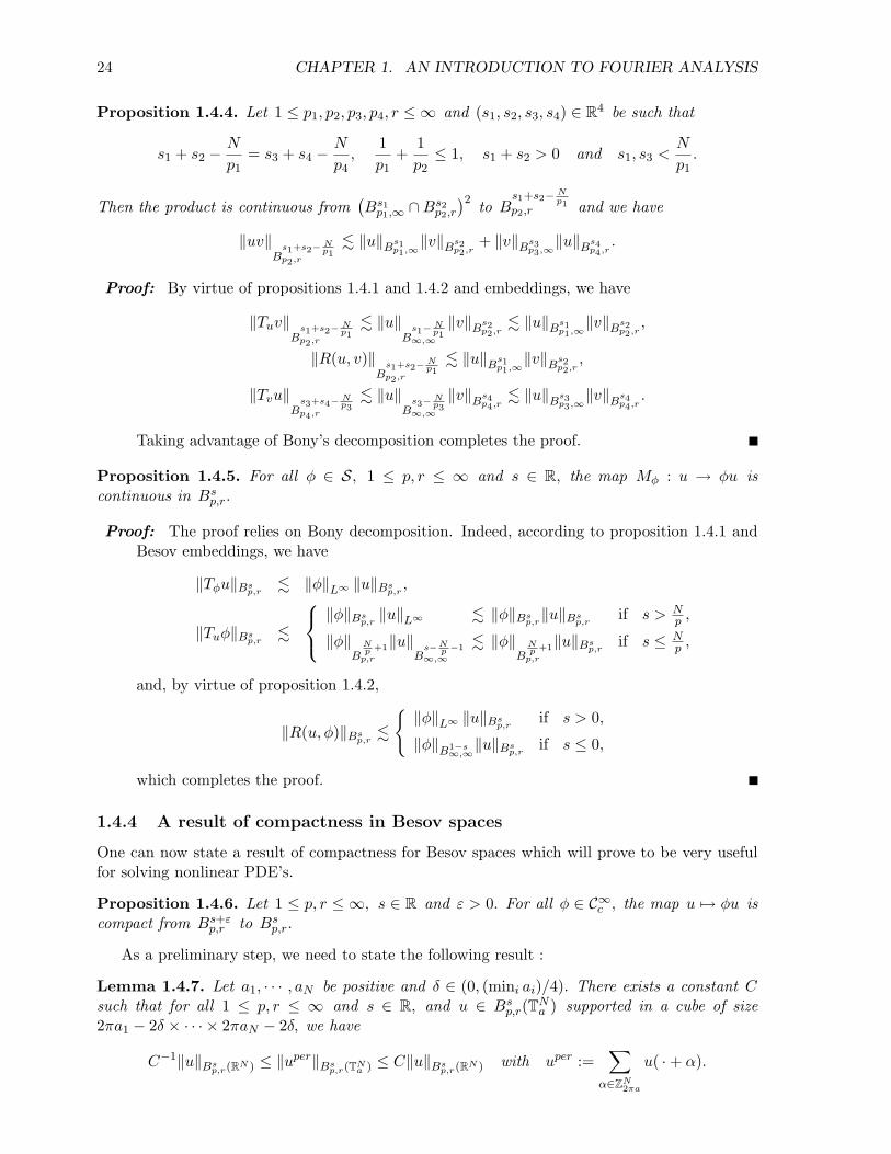
Proposition 1.4.4. Let 1 ≤ p1, p2, p3, p4, r ≤ ∞ and (s1, s2, s3, s4) ∈ R4 be such that

s1 + s2 −N

p1= s3 + s4 −

N

p4,

1p1

+1p2

≤ 1, s1 + s2 > 0 and s1, s3 <N

p1.

Then the product is continuous from(Bs1

p1,∞ ∩Bs2p2,r

)2 to Bs1+s2− N

p1p2,r and we have

‖uv‖B

s1+s2−Np1

p2,r

. ‖u‖Bs1p1,∞

‖v‖Bs2p2,r

+ ‖v‖Bs3p3,∞

‖u‖Bs4p4,r

.

Proof: By virtue of propositions 1.4.1 and 1.4.2 and embeddings, we have

‖Tuv‖B

s1+s2−Np1

p2,r

. ‖u‖B

s1−Np1∞,∞

‖v‖Bs2p2,r

. ‖u‖Bs1p1,∞

‖v‖Bs2p2,r

,

‖R(u, v)‖B

s1+s2−Np1

p2,r

. ‖u‖Bs1p1,∞

‖v‖Bs2p2,r

,

‖Tvu‖B

s3+s4−Np3

p4,r

. ‖u‖B

s3−Np3∞,∞

‖v‖Bs4p4,r

. ‖u‖Bs3p3,∞

‖v‖Bs4p4,r

.

Taking advantage of Bony’s decomposition completes the proof.

Proposition 1.4.5. For all φ ∈ S, 1 ≤ p, r ≤ ∞ and s ∈ R, the map Mφ : u → φu iscontinuous in Bs

p,r.

Proof: The proof relies on Bony decomposition. Indeed, according to proposition 1.4.1 andBesov embeddings, we have

‖Tφu‖Bsp,r

. ‖φ‖L∞ ‖u‖Bsp,r,

‖Tuφ‖Bsp,r

.

‖φ‖Bsp,r‖u‖L∞ . ‖φ‖Bs

p,r‖u‖Bs

p,rif s > N

p ,

‖φ‖B

Np +1

p,r

‖u‖B

s−Np −1

∞,∞

. ‖φ‖B

Np +1

p,r

‖u‖Bsp,r

if s ≤ Np ,

and, by virtue of proposition 1.4.2,

‖R(u, φ)‖Bsp,r

.

‖φ‖L∞ ‖u‖Bs

p,rif s > 0,

‖φ‖B1−s∞,∞

‖u‖Bsp,r

if s ≤ 0,

which completes the proof.

1.4.4 A result of compactness in Besov spaces

One can now state a result of compactness for Besov spaces which will prove to be very usefulfor solving nonlinear PDE’s.

Proposition 1.4.6. Let 1 ≤ p, r ≤ ∞, s ∈ R and ε > 0. For all φ ∈ C∞c , the map u 7→ φu iscompact from Bs+ε

p,r to Bsp,r.

As a preliminary step, we need to state the following result :

Lemma 1.4.7. Let a1, · · · , aN be positive and δ ∈ (0, (mini ai)/4). There exists a constant Csuch that for all 1 ≤ p, r ≤ ∞ and s ∈ R, and u ∈ Bs

p,r(TNa ) supported in a cube of size

2πa1 − 2δ × · · · × 2πaN − 2δ, we have

C−1‖u‖Bsp,r(RN ) ≤ ‖uper‖Bs

p,r(TNa ) ≤ C‖u‖Bs

p,r(RN ) with uper :=∑

α∈ZN2πa

u( ·+ α).

1.4. PARADIFFERENTIAL CALCULUS 25

Proof: With no loss of generality, one can assume that

Supp u ⊂ QNa,δ := [δ, 2πa1 − δ]× · · · × [δ, 2πaN − δ].

Let θ be a smooth function supported in QNa,δ/2 and equals to one on a neighborhood of

QNa,δ. Denoting hq := 2qNh(2q·), we have for all q ∈ N, M ∈ N and x ∈ RN ,

∆qu(x) = 〈u, θhq(x− ·)〉,=

⟨(Id−∆)−Mu, (Id−∆)M

(θhq(x− ·)

)⟩.

By virtue of Besov embeddings, one can choose M so large as to satisfy

Bsp,r(RN ) →

v ∈ S ′(RN ) | (Id−∆)−Mv ∈ L∞(RN )

.

By taking advantage of Leibniz formula, we thus get for some large enough C,

|∆qu(x)| ≤ C‖u‖Bsp,r(RN )

∑|α|+|β|≤2M

∫RN

|∂αθ(y)||∂βhq(x− y)| dy.

If one assumes that x 6∈ QNa then one has5 |x − y| ≥ |x − πa| − π|a| + δ/2 whenever y

belongs to Supp θ. Therefore one has for all K ∈ N,

|∆qu(x)| ≤C(

|x−πa|−π|a|+ δ2

)K ‖u‖Bsp,r(RN )

∑|α|+|β|≤2M

∫RN

|x−y|K |∂αθ(y)||∂βhq(x−y)| dy

and it is easy to conclude that there exists a constant CK such that

(1.15) |∆qu(x)| ≤ CK

(|x−πa| − π|a|+ δ

2)−K 2(2M−K)q‖u‖Bs

p,r(RN ) for all x∈RN \QNa .

By choosing K = 2M + 1 with M large enough, one can now easily conclude that

(1.16) ‖∆qu‖Lp(RN\QNa ) ≤ C2−q‖u‖Bs

p,r(RN )

for some constant C depending only on δ and on a.

Next, we notice that, by virtue of proposition 1.2.2, we have

∀x ∈ RN , ∆perq uper(x)−∆qu(x) =

∑α∈ZN

2πa\0

∆qu(x+ α).

Therefore, taking M large enough and using (1.15) with K = 2M + 1, one gathers thatfor all x ∈ QN

a , we have

|∆perq uper(x)−∆qu(x)| ≤ C2−q‖u‖Bs

p,r(RN ),

whence

(1.17) ‖∆perq uper −∆qu‖Lp(QN

a ) ≤ C2−q‖u‖Bsp,r(RN ).

Note that if one replaces the function hq by the function 2qNF−1χ(2q·) in the abovecomputations then one gets

(1.18) max(‖Squ‖Lp(RN\QN

a ), ‖Sperq uper−Squ‖Lp(QN

a )

)≤ C2−q‖u‖Bs

p,r(RN ).

5We take the max norm in RN to simplify the computations.

26 CHAPTER 1. AN INTRODUCTION TO FOURIER ANALYSIS

Let q0 ∈ N be such that 8C2−q0 ≤ 1. From (1.16), (1.17) and (1.18), we get∣∣∣∣∣(‖Sper

q0uper‖r

Lp(QNa ) +

∑q≥q0

(2qs‖∆per

q uper‖Lp(QNa )

)r) 1r

−(‖Sq0u‖r

Lp(RN ) +∑q≥q0

(2qs‖∆qu‖Lp(RN )

)r) 1r

∣∣∣∣∣ ≤ ‖u‖Bsp,r(RN )

2.

One can easily show that(‖Sper

q0uper‖r

Lp(QNa ) +

∑q≥q0

(2qs‖∆per

q uper‖Lp(QNa )

)r) 1r

≈ ‖uper‖Bsp,r(TN

a )

and that (‖Sq0u‖r

Lp(RN ) +∑q≥q0

(2qs‖∆qu‖Lp(RN )

)r) 1r

≈ ‖u‖Bsp,r(RN )

whence the desired result.

One can now prove proposition 1.4.6. According to proposition 1.4.5, we already know thatTφ : u 7→ φu maps Bs+ε

p,r (RN ) in Bsp,r(RN ). We shall prove the compactness by decomposing Tφ

into a product of continuous maps, one of them being compact.With no loss of generality, one can assume that φ is supported in some cube QN

a,δ whichsatisfies the assumptions of proposition 1.4.7. Now, one can use the decomposition

Tφ = J I Π Mφ

where

• J stands for the extension map by 0 outside QNa from the subset of those distributions

over TNa whose restriction to QN

a is supported in QNa,δ, to the set of temperate distributions

over RN supported in QNa,δ,

• I is the canonical embedding from Bs+εp,r (TN

a ) to Bsp,r(TN

a ),

• Π is the map u 7→ uper introduced in proposition 1.2.2,

• Mφ is the map u 7→ φu over Bs+εp,r (RN ) with values in Bs+ε

p,r (RN ).

According to proposition 1.4.5, the map Mφ is continuous. Besides, according to lemma 1.4.7,the map J (resp. Π ) is continuous from the subspace of those distributions of Bs

p,r(TNa ) whose

restriction to QNa is supported in QN

a,δ, to Bsp,r(RN ) (resp. from the subspace of distributions

of Bs+εp,r (RN ) supported in QN

a,δ, to Bs+εp,r (TN

a )).We claim that I may be approximated by a sequence of operators with finite rank. This

will yield compactness.Indeed, introduce the finite rank operator In defined by

In(v) :=∑q≤n

∆perq v.

Using proposition 1.2.1, we discover that for all q ∈ N, we have

∆perq (I − In)(v) =

∑j>n

|j−q|≤1

∆perq ∆per

v.

1.4. PARADIFFERENTIAL CALCULUS 27

We thus have for some constant C independent of q,

2qs‖∆perq (I − In)(v)‖Lp(TN

a ) ≤ C2−nε(2q(s+ε)‖∆per

q v‖Lp(TNa )

),

whence‖I − In)(v)‖Bs

p,r(TNa ) ≤ C2−nε‖v‖Bs+ε

p,r (TNa ).

This insures that In tends to I in L(Bs+ε

p,r (TNa );Bs

p,r(TNa )). The proof of proposition 1.4.6 is

complete.

1.4.5 Results of continuity for the composition

Let us state the main result of this section:

Proposition 1.4.8. Let I be an open interval of R. Let s > 0 and σ be the smallest integersuch that σ ≥ s. Let F : I → R satisfy F (0) = 0 and F ′ ∈ W σ,∞(I; R). Assume that v ∈ Bs

p,r

has values in J ⊂⊂ I . Then F (v) ∈ Bsp,r and there exists a constant C depending only on s,

I, J, and N, and such that

‖F (v)‖Bsp,r≤ C

(1+‖v‖L∞

)σ‖F ′‖Wσ,∞(I)‖v‖Bsp,r.

Proof: The proof is based on Meyer’s first linearization method (see e.g. [1], chapter 2).

Of course, one can change F for a function F ∈ Wσ+1,∞(R) compactly supported in Iand such that F ≡ F on a neighborhood of J . So let us assume that F belongs toWσ+1,∞(R) and has compact support in I.

The starting point of the proof is the following formal decomposition6

(1.19) F (v) =∑

q′≥−1

F (Sq′+1v)− F (Sq′v).

According to first order Taylor’s formula, we have for all q′ ≥ −1,

F (Sq′+1v)− F (Sq′v) = mq′∆q′v with mq′ :=∫ 1

0F ′(Sq′v + τ∆q′v) dτ.

One can easily prove that the mp ’s are Meyer multipliers, namely

(1.20) ∀k ∈ 0, · · · , σ,∥∥∥Dkmq′

∥∥∥L∞

≤ Ck2q′k(1 + ‖v‖L∞)k‖F ′‖Wk,∞ .

In particular, inequality (1.20) with k = 0 implies that∥∥F (Sq′+1v)− F (Sq′v)∥∥

Lp ≤ C2−q′s supq

2qs ‖∆qv‖Lp .

Since s is positive, we conclude that (1.19) holds true in Lp.

We now have to prove that F (v) belongs to Bsp,r. For all q ≥ −1, we have

∆qF (v) =∑

−1≤q′≤q−1

∆q

(mq′ ∆q′v

)︸ ︷︷ ︸

∆1q

+∑q′≥q

∆q

(mq′ ∆q′v

)︸ ︷︷ ︸

∆2q

.

6Remind that S−1v ≡ 0.

28 CHAPTER 1. AN INTRODUCTION TO FOURIER ANALYSIS

Taking advantage of Bernstein lemma, we get for all (q′, q) such that −1 ≤ q′ ≤ q − 1,∥∥∆q

(mq′ ∆q′v

)∥∥Lp . 2−qσ

∥∥Dσ∆q

(mq′ ∆q′v

)∥∥Lp ,

whence, combining Leibniz formula and (1.20),

2qs∥∥∆q

(mq′ ∆q′v

)∥∥Lp . ‖F ′‖Wσ,∞(I)(1 + ‖v‖L∞)σ 2(q′−q)(σ−s)

(2q′σ

∥∥∆q′v∥∥

Lp

).

Since σ > s, convolution inequalities enable us to conclude that(∑q

(2qs∥∥∆1

q

∥∥Lp

)r) 1r

. ‖F ′‖Wσ,∞(I)(1 + ‖v‖L∞)σ ‖v‖Bsp,r

and proposition 1.3.4 insures that∑

∆1q belongs to Bs

p,r.

Bounding the term pertaining to ∆2q is easy. Indeed, we have according to (1.20),

2qs∥∥∆q(mq′∆q′v)

∥∥Lp . ‖F ′‖L∞(I)2

(q−q′)s(2q′s

∥∥∆q′v∥∥

Lp

),

so that, since s > 0, (∑q

(2qs∥∥∆2

q

∥∥Lp

)r) 1r

. ‖F ′‖L∞(I) ‖v‖Bsp,r.

Applying once again proposition 1.3.4 completes the proof.

Finally, combining propositions 1.4.3 and 1.4.8 with the following equality:

F (v)− F (u) = (v − u)∫ 1

0F ′(u+ τ(v − u)) dτ,

we readily get the following

Corollary 1.4.9. Let I be an open interval of R and F : I → R. Let s > 0 and σ be thesmallest integer such that σ ≥ s. Assume that F ′(0) = 0 and that F ′′ belongs to Wσ,∞(I; R).Let u, v ∈ Bs

p,r have values in J ⊂⊂ I. There exists a constant C = Cs,I,J,N such that

‖F (v)− F (u)‖Bsp,r≤ C

(1+‖v‖L∞

)σ‖F ′′‖Wσ,∞(I)

×(‖v − u‖Bs

p,rsup

τ∈[0,1]‖u+ τ(v − u)‖L∞ + ‖v − u‖L∞ sup

τ∈[0,1]‖u+ τ(v − u)‖Bs

p,r

).

1.5 Calculus in homogeneous functional spaces

Nonhomogeneous functional spaces are not the most natural spaces for studying mathematicalproblems which have a property of invariance by dilation. For instance, it is well known thatthe Sobolev embedding H1(R3) → L6(R3) involves only the L2 norm of the gradient and notthe whole H1 norm. We shall also see in the next chapters that many interesting PDE’s havesome properties of scaling invariance.

This is a good motivation for introducing a homogeneous Littlewood-Paley decompositionwhere the low frequencies are treated exactly as the high frequencies, and to define homogeneousfunctional spaces.

1.5. CALCULUS IN HOMOGENEOUS FUNCTIONAL SPACES 29

1.5.1 Homogeneous Littlewood-Paley decomposition

Let (χ, ϕ) be as in section 1.2.2. The homogeneous dyadic blocks are defined by

∆qu := ϕ(2−qD)u for all q ∈ Z.

We also introduce the following low frequency cut-off:

Squ := χ(2−qD) for all q ∈ Z.

The above definition deserves two important preliminary remarks:

• For u ∈ S ′, we have∑

q∈Z ∆qu = u modulo a polynomial only.

• In contrast with the nonhomogeneous case, we do not have Squ =∑

p≤q−1 ∆pu.

In light of the first remark, working with distributions modulo polynomials seems to be the mostappropriate choice. As a matter of fact, this is the viewpoint of most authors of textbooks onabstract functional analysis (see e.g. [38] or [36]).

Since in the next chapters, we aim at applying homogeneous Littlewood-Paley decompositionfor solving nonlinear PDE’s however, it is not suitable to work with distributions defined modulopolynomials. This motivates the following definition (after J.-Y. Chemin in [12]):

Definition. We denote by S ′h the space of temperate distributions u such that

limj→−∞

Sju = 0 in S ′.

Remarks. (i) A polynomial u does not belong to S ′h unless it is identically 0. Indeed, if u isa polynomial then we have Sju = u for all j in Z .

(ii) It is obvious that S ′h is the space of temperate distributions u which satisfy

u =∑

j

∆ju in S ′.

(iii) The space S ′h is not a closed subspace of S ′ for the topology of weak convergence. Indeed,consider a sequence (fn)n∈N with fn(x) = f(x/n) and f ∈ S such that f(0) = 1. Then(fn)n∈N tends weakly to the constant function 1 which does not belong to S ′h.

Examples. (i) If a temperate distribution u is such that its Fourier transform u is locallyintegrable near 0, then u belongs to S ′h .

(ii) If u is a temperate distribution such that for some function θ in C∞c (RN ) with value 1near the origin, we have θ(D)u in Lp for some p ∈ [1,+∞[ , then u belongs to S ′h . Inparticular, when p if finite, any nonhomogeneous Besov space Bs

p,r is included in S ′h .

1.5.2 Homogeneous Besov spaces

Definition 1.5.1. Let u be a temperate distribution, s a real number, and 1 ≤ p, r ≤ ∞. Thenwe set

‖u‖Bsp,r

:=(∑

q∈Z2rqs‖∆qu‖r

Lp

) 1r

with the usual change if r = ∞.

For the semi-norms we have defined, we can prove the following inequalities

30 CHAPTER 1. AN INTRODUCTION TO FOURIER ANALYSIS

Theorem 1.5.2. A constant C exists such that for all s ∈ R,

r1 ≤ r2 ⇒ ‖u‖Bsp,r2

≤ ‖u‖Bsp,r1

,

p1 ≤ p2 ⇒ ‖u‖B

s−N( 1p1− 1

p2)

p2,r

≤ C‖u‖Bsp1,r

.

Moreover we have the following interpolation inequalities for any θ in ]0, 1[ and s < s:

‖u‖B

θs+(1−θ)esp,r

≤ ‖u‖θBs

p,r‖u‖1−θ

Besp,r,

‖u‖B

θs+(1−θ)esp,1

≤ C

θ(1− θ)(s− s)‖u‖θ

Bsp,∞‖u‖1−θ

Besp,∞

.

The proof is the same as in the nonhomogeneous framework, and thus omitted. Finally, thefollowing logarithmic interpolation inequalities are available:

Proposition 1.5.3. There exists a constant C such that for all s ∈ R, ε > 0 and 1 ≤ p ≤ ∞,we have

‖u‖Bsp,1

≤ C1+εε

‖u‖Bsp,∞

(1 + log

(‖u‖Bs−εp,∞

+ ‖u‖Bs+εp,∞

‖u‖Bsp,∞

)),(1.21)

‖u‖Bsp,1

≤ C1+εε

(1 + ‖u‖Bs

p,∞log(e+ ‖u‖Bs−ε

p,∞+ ‖u‖Bs+ε

p,∞

)).(1.22)

Proof: The proof is almost the same as in the nonhomogeneous framework. We write forsome positive integer Q to be fixed hereafter:

‖u‖Bsp,1

=∑

q≤−Q

2qs‖∆qu‖Lp +∑|q|<Q

2qs‖∆qu‖Lp +∑q≥Q

2qs‖∆qu‖Lp ,

whence, from elementary computations,

‖u‖Bsp,1≤ (2Q− 1)‖u‖Bs

p,∞+

2−Qε

1− 2−ε

(‖u‖Bs−ε

p,∞+ ‖u‖Bs+ε

p,∞

).

Choosing for Q the closest positive integer to1ε

log2

(‖u‖Bs−εp,∞

+ ‖u‖Bs+εp,∞

‖u‖Bsp,∞

)yields (1.21).

The second inequality may be easily deduced from (1.21).

Homogeneous Besov spaces have some invariance properties by dilation. More precisely, if forany temperate distribution u and λ > 0, we introduce the temperate distribution uλ definedfor all x ∈ RN by uλ(x) := u(λx), then we have

Proposition 1.5.4. If ‖u‖Bsp,r

is finite, so is ‖uλ‖Bsp,r

and we have

‖uλ‖Bsp,r≈ λ

s−Np ‖u‖Bs

p,r.

Besides, equality is true if λ = 2m for some m ∈ Z.

Proof: Let α be a positive real. We have

ϕ(α−1D)uλ(x) = αN

∫h(α(x− y))u(λy) dy.

1.5. CALCULUS IN HOMOGENEOUS FUNCTIONAL SPACES 31

By the change of variables z = λy , we get that

ϕ(α−1D)uλ(x) = αNλ−N

∫h(αx− αλ−1z)u(z) dz,

=[ϕ(λα−1D)u

](αx).

For q ∈ Z, let us denote vq := ϕ(2[log2 λ]−log2 λ−qD)uλ. Taking α = 2q−[log2 λ]λ in the aboveequality, we get

2qs‖vq‖Lp ≈ λs−N

p 2(q−[log2 λ])s‖∆q−[log2 λ]u‖Lp

with an equality if log2 λ is an integer.

Thus we deduce that (∑q

(2qs ‖vq‖Lp

)) 1r

≈ λs−N

p ‖u‖Bsp,r.

Since Supp vq ⊂ C(0, 342q, 16

3 2q), we have

∆quλ =∑

|p−q|≤2

∆puq.

Now, straightforward computations yield the desired result.

Next, we notice that ‖ · ‖Bsp,r

is actually only a semi-norm in the sense that, if u is a polynomial

then, for any integer q we have ∆qu = 0, (because the support of u is the origin), and so‖u‖Bs

p,r= 0. Therefore, if we define the homogeneous Besov space Bs

p,r as the set of temperatedistributions u such that ‖u‖Bs

p,ris finite, we may run into troubles later when studying non

linear problems because we will not be able to tell a polynomial from a null function !In the present lecture notes, we adopt the following definition:

Definition. Let s be a real number and (p, r) be in [1,∞]2 . The space Bsp,r is the set of

distributions u in S ′h such that ‖u‖Bsp,r

is finite.

In the homogeneous framework, the results corresponding to proposition 1.3.4 read:

Proposition 1.5.5. Let s ∈ R and 1 ≤ p, r ≤ ∞ satisfy

(1.23) s <N

p, or s =

N

pand r = 1.

(i) Let (uq)q∈Z be a sequence of functions such that(∑q

(2qs ‖uq‖Lp

)r) 1r

<∞.

If Supp uq ⊂ C(0, 2qR1, 2qR2) for some 0 < R1 < R2 then u :=∑

q∈Z uq belongs to Bsp,r

and there exists a constant C such that

(1.24) ‖u‖Bsp,r≤ C1+|s|

(∑q

(2qs ‖uq‖Lp

)r) 1r

.

Let (uq)q∈Z be a sequence of functions such that(∑q

(2qs ‖uq‖Lp

)r) 1r

<∞.

32 CHAPTER 1. AN INTRODUCTION TO FOURIER ANALYSIS

If Supp uq ⊂ B(0, 2qR) for some positive R and if in addition s is positive then u :=∑q∈Z uq belongs to Bs

p,r and there exists a constant C such that

(1.25) ‖u‖Bsp,r≤ C1+s

s

(∑q

(2qs ‖uq‖Lp

)r) 1r

.

Proof: Let us prove (i).

On one hand, using Bernstein lemma, it is easy to see that the series∑

q≤0 uq is convergentin L∞ and that u− :=

∑q≤0 uq belongs to S ′h. On the other hand, since ‖uq‖L∞ ≤

C2q(Np−s)

, lemma 1.3.3 insures that the series∑

q>0 uq is convergent in S ′. Besides, theFourier transform of u+ :=

∑q>0 uq is supported away from the origin, hence u+ belongs

to S ′h. Since u = u− + u+, one can conclude that u belongs to S ′h. Now, the proof of(1.24) may be done exactly as in lemma 1.3.4.

Proving (ii) is similar. Indeed, we have for any q ∈ Z,

‖uq‖Lp ≤ C2−qs and ‖uq‖L∞ ≤ C2q(Np−s)

.

Hence∑

q≤0 uq converges in L∞ and belongs to S ′h whereas∑

q>0 uq converges in Lp

(and also belongs to S ′h since its Fourier transform is bounded away from 0). Next, theproof of (1.25) goes along the lines of lemma 1.3.4.

As an important corollary of proposition 1.5.5, we get that, under condition (1.23), the definitionof Bs

p,r does not depend on ϕ.

The following proposition, the proof of which is left to the reader, describes the relationsbetween homogeneous and nonhomogeneous spaces.

Proposition 1.5.6. Let s be a negative number (or s = 0 and r = 1). Then Bsp,r → Bs

p,r.

Besides, if s < 0, a constant C (independent of s) exists so that, for any u belonging to Bsp,r ,

we have‖u‖Bs

p,r≤ C

−s‖u‖Bs

p,r.

Let s be a positive number (or s = 0 and r = ∞). Then Bsp,r → Bs

p,r when p is finite, andBs∞,r ∩S ′h is a subset of Bs

∞,r. If s > 0, a constant C exists (independent of s) so that, for anyu belonging to Bs

p,r , we have

‖u‖Bsp,r≤ C

s‖u‖Bs

p,r.

Let us notice that there is no monotonicity property with respect to s for homogeneousspaces. The reason why is that homogeneous Besov spaces carry on informations about bothlow and high frequencies.

In homogeneous spaces, the counterpart of proposition 1.3.8 reads:

Proposition 1.5.7. There exists a constant C which satisfies the following properties. Lets < 0, (p, r) ∈ [1,∞]2 and u a distribution in S ′h . Then u belongs to Bs

p,r if and only if

(2qs‖Squ‖Lp)q∈Z ∈ `r(Z).

Moreover, we have

12‖u‖Bs

p,r≤(∑

q

(‖(2qs‖Squ‖Lp)q

)r) 1r

≤ C(1 +

1|s|

)‖u‖Bs

p,r.

1.5. CALCULUS IN HOMOGENEOUS FUNCTIONAL SPACES 33

Proof: The proof goes along the lines of proposition 1.3.8.

Proposition 1.5.8. Let f be a smooth function on RN \ 0 which is homogeneous of degreem. Let 1 ≤ p, r ≤ ∞. Assume that

s−m <N

p, or r = 1 and s−m ≤ N

p·

Then f(D) is continuous from Bsp,r to Bs−m

p,r .

Proof: Assume that r > 1. Introduce a smooth function ϕ supported in a shell and suchthat ϕ ≡ 1 on Supp ϕ. As f is homogeneous of degree m , we have

∆qf(D)u = 2qm[ϕf ](2−qD)∆qu.

Since F−1(ϕf) belongs to S, we readily get∥∥∥∆qf(D)u∥∥∥

Lp≤ C2qm

∥∥∥∆qu∥∥∥

Lp,

whence (∑q

(2q(s−m)‖∆qf(D)u‖Lp

)r) 1r

. ‖u‖Bsp,r.

Now, we haveSqf(D)u =

∑q′≤q

Sqf(D)∆q′u,

whence according to Bernstein lemma,∥∥∥Sqf(D)u∥∥∥

L∞.∑q′≤q

2q′(Np

+m−s)2q′s∥∥∥∆q′u

∥∥∥Lp

. 2q(Np

+m−s)‖u‖Bsp,∞

.

Since N/p + m − s > 0, it is now clear that Sqf(D)u tends to 0 when q goes to −∞.Hence f(D)u belongs to Bs−m

p,r . The proof in the case r = 1 is left to the reader.

Let us now focus on the topological properties of the spaces Bsp,r.

Proposition 1.5.9. For all s ∈ R and 1 ≤ p, r ≤ ∞, the couple (Bsp,r, ‖ · ‖Bs

p,r) is a normed

space. If besides r is finite then C∞c ∩ Bsp,r is densely embedded in Bs

p,r.

Proof: It is obvious that ‖ · ‖Bsp,r

is a semi-norm. Let us assume that ‖u‖Bsp,r

= 0 for some

u in S ′h. This implies that Supp u ⊂ 0 and thus that for any j ∈ Z we have Sju = u.As u belongs to S ′h, we must have lim

j→−∞Sju = 0 so that we can conclude that u = 0.

Now, if r is finite and u ∈ Bsp,r, it is obvious that the sequence of general term∑

|q|≤n

∆qu

belongs to C∞ ∩ Bsp,r and tends to u in Bs

p,r. Arguing like in 1.3.5.(ii), it is then easy toexhibit a sequence of functions of C∞c ∩ Bs

p,r which tends to u in Bsp,r.

Theorem 1.5.10. If s < Np or s = N

p and r = 1 then (Bsp,r, ‖ · ‖Bs

p,r) is a Banach space which

is continuously embedded in S ′.

34 CHAPTER 1. AN INTRODUCTION TO FOURIER ANALYSIS

Proof: Let us first prove that Bsp,r is continuously embedded in S ′ . The case r = 1 and

s = N/p is easy because the series∑

∆ju is convergent in L∞. As u =∑

j ∆ju, thisimplies that u belongs to L∞ . Besides, we have

(1.26) BNp

p,1 → B0∞,1 → L∞ → S ′.

Let us now assume that s < N/p. Using that Bsp,r → B

s−Np

∞,∞ and arguing like for proving(1.10), one can find a large integer M such that for all nonnegative j, we have

|〈∆ju, φ〉| ≤ 2−j‖u‖B

s−Np

∞,∞

‖φ‖M,S .

For negative j , one can write that for large enough M , we have

|〈∆ju, φ〉| . 2j“

Np−s

”‖u‖

Bs−N

p∞,∞

‖φ‖L1

. 2j“

Np−s

”‖u‖Bs

p,r‖φ‖M,S .

Because u belongs to S ′h , we have 〈u, φ〉 =∑

j〈∆ju, φ〉. Therefore, for large enough M ,

(1.27) |〈u, φ〉| ≤ Cs‖u‖Bsp,r‖φ‖M,S

and we can conclude that Bsp,r → S ′.

We still have to prove that for all triplet (s, p, r) satisfying the hypothesis of the theorem,the set Bs

p,r is a Banach space. So let us consider a Cauchy sequence (un)n∈N in Bsp,r.

Using (1.26) or (1.27), this implies that a temperate distribution u exists such that thesequence (un)n∈N converges to u in S ′ . We now have to state that u belongs to S ′h . Letus first assume that s < N/p. Since un belongs to S ′h, we have, thanks to (1.27),

∀j ∈ Z , ∀n ∈ N , |〈Sjun, φ〉| . 2j“

Np−s

”‖un‖Bs

p,r‖φ‖M,S .

As the sequence (un)n∈N tends to u in S ′ , we have

∀j ∈ Z , |〈Sju, φ〉| ≤ Cs2j“

Np−s

”‖φ‖M,S sup

n‖un‖Bs

p,r.

Thus u belongs to S ′h .

The case when u belongs to BNp

p,1 is a little bit different. Let ε > 0. As (un)n∈N is a

Cauchy sequence in BNp

p,1 → B0∞,1 , there exists an integer n0 such that

∀j ∈ Z , ∀n ≥ n0 ,∑k≤j

‖∆kun‖L∞ ≤ ε

2+∑k≤j

‖∆kun0‖L∞ .

Let us choose j0 small enough so that∑k≤j0

‖∆kun0‖L∞ ≤ ε

2·

As un belongs to S ′h , we have

∀j ≤ j0 , ∀n ≥ n0 , ‖Sjun‖L∞ ≤ ε.

1.5. CALCULUS IN HOMOGENEOUS FUNCTIONAL SPACES 35

As sequence (un)n∈N tends to u in L∞ , this implies that

∀j ≤ j0 , ‖Sju‖L∞ ≤ ε.

This proves that u belongs to S ′h . Next, arguing like in the nonhomogeneous case com-pletes the proof.

Remark. It turns out that when s > N/p (or s = N/p and r > 1) the space Bsp,r is no longer a

Banach space. In the one dimensional case for instance, it is can be easily seen that the sequence(fn)n∈N defined by

fn(ξ) =χ(ξ)ξ log |ξ|

if |ξ| ≥ 2−n, and 0 elsewhere,

is a Cauchy sequence in B122,∞ but cannot have a limit in B

122,∞ since the function ξ 7→ χ(ξ)

ξ log |ξ|does not belong to S ′ !

This defect of convergence due to low frequencies is typical to homogeneous functional spaceswith high regularity index. It is sometimes called infrared divergence.

There is a way to modify the definition of homogeneous Besov spaces so as to get a Banachspace regardless of the regularity index. This is called realizing homogeneous Besov spaces. Itturns out that realizations coincide with definition 1.5.2 when s < N/p or s = N/p and r = 1.In the other cases however, realizations are not functional spaces but spaces defined up to apolynomial whose degree depends on s − N/p and on r (see e.g [5] or [32]). It goes withoutsaying that solving PDE’s in such spaces may be quite unpleasant.

1.5.3 Paradifferential calculus in homogeneous spaces

We designate homogeneous paraproduct of v by u and denote by Tuv the bilinear operator:

Tuv :=∑

q

Sq−1u ∆qv.

We designate homogeneous remainder of u and v and denote by R(u, v) the bilinear operator:

R(u, v) =∑

|p−q|≤1

∆pu ∆qv.

It is clear that, formally, we have the following homogeneous Bony decomposition:

(1.28) uv = Tuv + Tvu+ R(u, v).

The properties of continuity of homogeneous paraproduct and remainder on homogeneous Besovspaces are described in the following propositions.

Proposition 1.5.11. There exists a constant C such that for any couple of real numbers (s, σ)with σ positive and for any (p, r, r1, r2) in [1,+∞]4 with 1/r = 1/r1 + 1/r2, we have

‖T‖L(L∞×Bsp,r;Bs

p,r) ≤ C |s|+1

if condition (1.23) is satisfied, and

‖T‖L(B−σ∞,r1

×Bsp,r2

;Bs−σp,r ) ≤

C |s−σ|+1

σ·

if s− σ < N/p, or s− σ = N/p and r = 1.

36 CHAPTER 1. AN INTRODUCTION TO FOURIER ANALYSIS

Proof: Let wq := Sq−1u ∆qv. Arguing like in proposition 1.4.1, one can easily prove that(∑q

(2qs ‖wq‖Lp

)r) 1r

. ‖u‖L∞ ‖v‖Bsp,r

and(∑

q

(2q(s−σ) ‖wq‖Lp

)r) 1r

. ‖u‖B−σ∞,r1

‖v‖Bsp,r2

.

Since the sequence (Fwq)q∈Z is supported in dyadic shells, applying proposition 1.5.5completes the proof.

Proposition 1.5.12. There exists a constant C which satisfies the following inequalities. Forany (s1, s2), any 1 ≤ p1, p2, p ≤ ∞ and any 1 ≤ r, r1, r2 ≤ ∞ such that

s1 + s2 > 0,1p≤ 1p1

+1p2

≤ 1 and1r≤ 1r1

+1r2≤ 1,

we have

‖R‖L(Bs1p1,r1

×Bs2p2,r2

;Bσ12p,r ) ≤

C |s1+s2|+1

s1 + s2with σ12 := s1 + s2 −N

(1p1

+1p2

− 1p

),

provided that σ12 < N/p, or σ12 = N/p and r = 1.

Proof: Denoting wq := ∆qu ∆qv and arguing like in proposition 1.4.2, we easily get(∑q

(2qσ12 ‖wq‖Lp

)r) 1r

. ‖u‖Bs1p1,r1

‖v‖Bs2p2,r2

.

Since the sequence the sequence (Fwq)q∈Z is supported in dyadic balls, applying proposi-tion 1.5.5 completes the proof.

Proposition 1.5.13. Let I be an open interval of R. Let s > 0 and σ be the smallest integersuch that σ ≥ s. Let F : I → R satisfy F (0) = 0 and F ′ ∈ Wσ,∞(I; R). Assume that v ∈ Bs

p,r

has values in J ⊂⊂ I. Assume that condition (1.23) is satisfied. Then F (v) ∈ Bsp,r and there

exists a constant C = Cs,I,J,N such that

‖F (v)‖Bsp,r≤ C

(1+‖v‖L∞

)σ‖F ′‖Wσ,∞(I)‖v‖Bsp,r.

Proof: Arguing like in the proof of proposition 1.4.8 and using Bernstein lemma, we get forall j ∈ Z, ∥∥∥F (Sj+1v)− F (Sjv)

∥∥∥Lp≤ C2−js

(2js ‖∆jv‖Lp

),∥∥∥F (Sj+1v)− F (Sjv)

∥∥∥L∞

≤ C2j(Np−s) (2js ‖∆jv‖Lp

).

Since s is positive, F (0) = 0 and condition (1.23) is satisfied, this insures that the series∑j∈Z

F (Sj+1v)− F (Sjv)

converges to F (v) in Lp + L∞, thus in S ′.Next, for all q ∈ Z, we split ∆qF (v) into

∆qF (v) =∑j<q

∆q(mj∆jv) +∑j≥q

∆q(mj∆jv).

Following the lines of the proof of proposition 1.4.8 and applying proposition 1.5.5 leadsto the desired result.

1.6. EXERCISES 37

1.6 Exercises

Exercise 1.1. Prove that for any α > 1, there exists two smooth functions ϕ and χ suchthat ϕ is supported in the shell ξ ∈ RN |α−1 ≤ |ξ| ≤ 2α and χ is supported in the ballξ ∈ RN | |ξ| ≤ α, and

∀ξ ∈ RN , χ(ξ) +∑q∈N

ϕ(2−qξ) = 1.

Exercise 1.2. Prove that for all temperate distribution u, the equality u =∑

q∈Z ∆qu holdstrue in S ′(RN ).

Exercise 1.3. Prove proposition 1.2.1.

Exercise 1.4. Prove inequality (1.5).

Exercise 1.5. For q ∈ Z, denote ∆′qu := 12q≤|ξ|≤2q+1(D)u. Prove that the inequality∥∥∆′

qu∥∥

Lp ≤ C ‖u‖Lp

for some constant C independent of q is false in the case p 6= 2.Hint: Try with the function u = χ.

Exercise 1.6. Compare the Besov space B0p,r with the Lebesgue space Lp.

Exercise 1.7. Let Bsp,∞ be the completion of C∞c for the ‖ · ‖Bs

p,∞ norm. Prove that u ∈ Bsp,∞

if and only if limq→+∞ 2qs ‖∆qu‖Lp = 0.

Exercise 1.8. Let r ∈ (0, 1). Prove that Br−1∞,∞(RN ) is the set of temperate distributions u

such that there exist N + 1 functions u0, · · · , uN of Cr verifying

u = u0 +N∑

j=1

∂juj .

Exercise 1.9. Let C1? be the Zygmund space of bounded functions u such that

∀(x, y) ∈ RN × RN , |u(x+ y) + u(x− y)− 2u(x)| ≤ C|y|

for some constant C.Prove that C1

? = B1∞,∞.

Exercise 1.10. Let 1 ≤ p, p1, p2, r ≤ ∞ and s ∈ R . Let r′ := r/(r − 1). Assume that1/p ≤ 1/p1 + 1/p2.

Prove that the remainder R maps Bsp1,r ×B−s

p2,r′ in B−N(

1p− 1

p1− 1

p2

)p,∞ .

Exercise 1.11. Prove (1.20).

Exercise 1.12. Let I be an open interval of R and F : I → R. Assume that F (0) = 0 andthat F ′ is bounded.

Prove that for all v ∈ B0p,1 with values in J ⊂⊂ I , the function F (v) belongs to B0

p,1 andthat

‖F (v)‖B0p,1

. ‖F ′‖L∞(I)‖v‖B0p,1.

Exercise 1.13. Prove that u belongs to S ′h if and only if for any θ in C∞c (RN ) with value 1near the origin, we have lim

λ→∞θ(λD)u = 0 in S ′ .

38 CHAPTER 1. AN INTRODUCTION TO FOURIER ANALYSIS

Exercise 1.14. Prove proposition 1.5.6.

Exercise 1.15. We say that a temperate distribution u tends weakly to 0 at infinity if u(λ ·)tends to 0 in S ′ when λ goes to infinity.

Prove that u ∈ S ′ belongs to S ′h if and only if u tends weakly to 0 at infinity.

Exercise 1.16. Let s be in ]0, N [ . Prove that for any p in [1,∞], we have

1| · |s

∈ BNp−s

p,∞ .

Exercise 1.17. Find divergent Cauchy sequences for the space Bsp,r when s > N/p or s = N/p

and r > 1.

Exercise 1.18. Let 1 ≤ p1, r1, p2, r2 ≤ ∞ and (s1, s2) ∈ R2. Assume that

s1 <N

p1or s1 =

N

p1and r1 = 1.

Prove that Lp1 ∩ Bs2p2,r2

and Bs1p1,r1

∩ Bs2p2,r2

are Banach spaces.

Exercise 1.19. Let 1 ≤ p, r ≤ +∞, s ∈ R and ε > 0. Let φ ∈ C∞c (RN ).Prove that the map u 7→ φu is compact from Bs

p,r to Bs−εp,r + Bs

p,r.

Exercise 1.20. Let s be a positive real number and (p, r) ∈ [1,∞]2 . Prove the existence of aconstant C such that for all u in S ′h , we have

C−1‖u‖B−2sp,r

≤∥∥∥‖tset∆u‖Lp

∥∥∥Lr(R+, dt

t)≤ C‖u‖B−2s

p,r.

Hint: use that for any positive s and c, we have

supt>0

∑j∈Z

ts22jse−ct22j<∞.

Exercise 1.21. Let s be in ]0, 1[ and (p, r) ∈ [1,∞]2 . Prove that there exists a constant Csuch that for any u in S ′h, we have

C−1‖u‖Bsp,r≤∥∥∥‖τ−zu− u‖Lp

|z|s∥∥∥

Lr(RN ; dz

|z|N)≤ C‖u‖Bs

p,r

Exercise 1.22. 1) Let (s1, s2), (p1, p2, p) and (r1, r2) be such that

s1 + s2 ≥ 0,1p≤ 1p1

+1p2

≤ 1 and1r1

+1r2

= 1.

Assume that σ12 := s1 + s2 − N(

1p1

+ 1p2− 1

p

)satisfies σ12 < N/p, or σ12 = N/p and

r = 1.

Prove that the remainder is continuous from Bs1p1,r1

×Bs2p2,r2

to Bσ12p,∞ and that

‖R‖L(Bs1p1,r1

×Bs2p2,r2

;Bσ12p,∞) ≤ C |s1+s2|+1.

2) Adapt exercise 1.12 to the homogeneous framework.

Chapter 2

The heat equation

In this chapter, we state estimates in Besov spaces for the heat equation. Such estimates arefundamental for solving certain nonlinear PDE’s of parabolic type. As an example, we showthat incompressible Navier-Stokes equations are locally well-posed in Besov spaces with criticalindex of regularity.

2.1 Generalities

The basic heat equation reads

(H)∂tu− µ∆u = f,u|t=0 = u0.

Above, the external source term f = f(t, x) and the initial data u0 = u0(x) are given. Thediffusion µ is a positive constant. We restrict ourselves to the evolution for positive times t,and, for the sake of simplicity, we always assume that x belongs to the whole space RN . Similarresult would hold in the torus TN

a , though.Giving an exhaustive list of properties of the heat equation is not our goal here. We however

have to recall a few important facts for (H) that will be needed for stating estimates in Besovspaces.

Let u0 ∈ S(RN ) and f ∈ C(R+;S(RN )). Applying the partial Fourier transform with respectto the space variable (still denoted by ), we get the following linear ordinary differentialequation for all ξ ∈ RN :

(H)∂tu(t, ξ) + µ|ξ|2u(t, ξ) = f(t, ξ),u|t=0(ξ) = u0(ξ),

whence

(2.1) u(t, ξ) = e−µ|ξ|2tu0(ξ) +∫ t

0e−µ|ξ|2(t−τ)f(τ, ξ) dτ.

Performing the inverse Fourier transform, we end up with the following well known representationformula for all t ∈ R+ and x ∈ RN :

(2.2) u(t, x) =1

(4πµt)N2

∫RN

e− |x−y|2

4µt u0(y) dy +∫ t

0

1

(4πµ(t−τ))N2

(∫RN

e− |x−y|2

4µ(t−τ) f(τ, y) dy)dτ.

By arguing by duality, formulae (2.1) and (2.2) may be extended to temperate distributions.

39

40 CHAPTER 2. THE HEAT EQUATION

Introducing the heat semi-group(es∆)s≥0

for the Laplacian operator, equality (2.2) may berewritten in a more concise way:

(2.3) u(t) = eµt∆u0 +∫ t

0eµ(t−τ)∆f(τ) dτ.

Although formulae (2.1) and (2.2) are explicit, they are not so convenient for getting a prioriestimates in functional spaces. In fact, even for stating the basic energy equality, it is far moreefficient to multiply (H) by u, integrate over RN and perform an integration by parts in theterm with the Laplacian. At least formally, we end up with

12d

dt‖u‖2

L2 + µ ‖Du‖2L2 =

∫fu dx,

thus, integrating over the time interval [0, T ], we get

‖u(T )‖2L2 + 2µ

∫ T

0‖Du(t)‖2

L2 dt = ‖u0‖2L2 + 2

∫ T

0

∫RN

f(t, x)u(t, x) dt dx.

We notice that starting from u0 ∈ L2 and f ∈ L2(0, T ; H−1), the above equality provides anestimate for Du in L2(0, T × RN ). In other words, it gives a gain of one derivative for u withrespect to u0 and of two derivatives with respect to f. One can wonder if it is possible to gainmore than one derivative with respect to u0 by considering Lρ norms in time (ρ < 2) withvalues in Sobolev spaces.

In the next section, we shall see that very simple arguments based on Littlewood-Paleydecomposition enable us to gain two derivatives when taking a L1 norm in time. Besides, themethod we are going to present apply indistinctly to the Lp framework for all p ∈ [1,+∞].

2.2 A priori estimates in Besov spaces for the heat equation

The fundamental idea is to localize the heat equation through a Littlewood-Paley decomposition.It is then easy to prove Lρ(0, T ;Lp) estimates for each dyadic block in term of norms of ∆qu0

and ∆qf. If one assumes that u0 and f belong to some Besov spaces, performing a (weighted)`r summation is the most natural next step. In doing so however, one does not obtain anestimate in a space of type Lρ(0, T ; Bs

p,r) since the time integration has been performed beforethe summation.

This leads to the definition of the following spaces first introduced by J.-Y. Chemin and N.Lerner in [13] then extended in [9].

Definition. For T > 0, s ∈ R, 1 ≤ r, ρ ≤ ∞, we set (with the usual convention if r = ∞):

‖u‖eLρT (Bs

p,r):=(∑

q

(2qs‖∆qu‖Lρ

T (Lp)

)r) 1r

.

We then define the space LρT (Bs

p,r) as the set of temperate distributions u over (0, T ) × RN

such that limq→−∞

Squ = 0 in S ′(0, T × RN ) and ‖u‖eLρT (Bs

p,r)<∞.

In a similar way, we set

‖u‖eLρ(Bsp,r)

:=(∑

q

(2qs‖∆qu‖Lρ(R+;Lp)

)r) 1r

,

and define the space Lρ(Bsp,r) as the set of temperate distributions u over R+ × RN such that

limq→−∞

Squ = 0 in S ′(R+ × RN ) and ‖u‖eLρ(Bsp,r)

<∞.

2.2. A PRIORI ESTIMATES IN BESOV SPACES FOR THE HEAT EQUATION 41

Remark 2.2.1. (i) According to Minkowski inequality, we have

‖u‖eLρT (Bs

p,r)≤ ‖u‖Lρ

T (Bsp,r) if r ≥ ρ, ‖u‖eLρ

T (Bsp,r)

≥ ‖u‖LρT (Bs

p,r) if r ≤ ρ.

(ii) All the properties of continuity for the product, composition, remainder and paraproductstated in chapter 1 may be easily generalized to the spaces Lρ

T (Bsp,r). The general principle

is that the time exponent ρ behaves according to Holder inequality.

For instance, we have the following tame estimate :

‖uv‖eLρT (Bs

p,r). ‖u‖L

ρ1T (L∞)‖v‖eLρ2

T (Bsp,r)

+ ‖v‖Lρ3T (L∞)‖u‖eLρ4

T (Bsp,r)

whenever s > 0, 1 ≤ p ≤ ∞, 1 ≤ ρ, ρ1, ρ2, ρ3, ρ4 ≤ ∞ and

1ρ

=1ρ1

+1ρ2

=1ρ3

+1ρ4·

Remark. Of course similar definitions may be given in the nonhomogeneous framework, leadingto some functional spaces denoted by Lρ

T (Bsp,r). The details are left to the reader.

2.2.1 Spectral localization

In this section, we prove estimates for the semi-group of the heat equation restricted to functionswith compact supports away from the origin in Fourier variables. These estimates are based onthe following result.

Lemma 2.2.2. Let φ be a smooth function supported in the shell C(0, R1, R2) with 0 < R1 < R2.There exist two positive constants κ and C depending only on φ and such that for all 1 ≤ p ≤ ∞,τ ≥ 0 and λ > 0, we have∥∥φ(λ−1D)eτ∆u

∥∥Lp ≤ Ce−κτλ2 ∥∥φ(λ−1D)u

∥∥Lp .

Proof: Performing a change of variable, one can assume with no loss of generality that λ = 1.Now, let φ be a smooth function supported in C(0, R′1, R

′2) for some R′1 < R1 and R′2 > R2

and such that φ ≡ 1 in a neighborhood of C(0, R1, R2). We have

F(φ(D)eτ∆u

)(ξ) =

(φ(ξ)e−τ |ξ|2

)F(φ(D)u)(ξ).

Thus, φ(D)eτ∆u = kτ ? φ(D)u with

kτ (z) := (2π)−N

∫RN

e−τ |ξ|2eiz·ξφ(ξ) dξ.

According to convolution inequalities, we have∥∥φ(D)eτ∆u∥∥

Lp ≤ ‖kτ‖L1 ‖φ(D)u‖Lp .

Therefore it only remains to prove that there exist two positive constants κ and C suchthat

(2.4) ∀τ ∈ R+, ‖kτ‖L1 ≤ Ce−κτ .

For that, we use the fact that for all m ∈ N, we have

(1 + |z|2)mkτ (z) = (2π)−N

∫e−τ |ξ|2 φ(ξ) (Id−∆ξ)m

(eiz·ξ

)dξ,

= (2π)−N

∫eiz·ξ (Id−∆ξ)m

(e−τ |ξ|2 φ(ξ)

)dξ.

42 CHAPTER 2. THE HEAT EQUATION

From the last equality and the fact that the integration may be restricted to the shellC(0, R′1, R

′2), we easily conclude that there exists a constant Cm such that

∀z ∈ RN , (1 + |z|2)m|kτ (z)| ≤ Cme−κτ ,

whence inequality (2.4).

2.2.2 Estimates for the heat equation

Let us now state our main result for the heat equation.

Theorem 2.2.3. Let T > 0, s ∈ R and 1 ≤ ρ, p, r ≤ ∞. Assume that u0 ∈ Bsp,r and

f ∈ LρT (B

s−2+ 2ρ

p,r ). Then (H) has a unique solution u in LρT (B

s+ 2ρ

p,r )∩ L∞T (Bsp,r) and there exists

a constant C depending only on N and such that for all ρ1 ∈ [ρ,+∞], we have

µ1

ρ1 ‖u‖eLρ1T (B

s+ 2ρ1

p,r )≤ C

(‖u0‖Bs

p,r+ µ

1ρ−1‖f‖eLρ

T (Bs−2+ 2

ρp,r )

).

If in addition r is finite then u belongs to C([0, T ]; Bsp,r).

Proof: Since u0 and f are temperate distributions, equation (H) has a unique solution u inS ′(0, T × RN ), which satisfies

u(t, ξ) = e−µt|ξ|2 u0(ξ) +∫ t

0e−µ(t−τ)f(τ, ξ) dτ.

As F(Squ0) (resp. F(Sqf)) tends to 0 in S ′(RN ) (resp. S ′(0, T × RN )) when q goes to−∞, we easily gather that also Squ goes to zero in S ′(0, T × RN ) when q goes to −∞.

Next, we notice that, applying ∆q to (H) and using formula (2.3) yields

∆qu(t) = eµt∆∆qu0 +∫ t

0eµ(t−τ)∆qf(τ) dτ.

Therefore, ∥∥∥∆qu(t)∥∥∥

Lp≤∥∥∥eµt∆∆qu0

∥∥∥Lp

+∫ t

0

∥∥∥eµ(t−τ)∆∆qf(τ)∥∥∥

Lpdτ.

By virtue of lemma 2.2.2, we thus have for some κ > 0,∥∥∥∆qu(t)∥∥∥

Lp. e−κµ22qt ‖∆qu0‖Lp +

∫ t

0e−κµ22q(t−τ)

∥∥∥∆qf(τ)∥∥∥

Lpdτ.

Applying convolution inequalities, we get

‖∆qu‖Lρ1T (Lp) .

(1− e−κµTρ122q

κµρ122q

) 1ρ1

‖∆qu0‖Lp +(

1− e−κµTρ222q

κµρ222q

) 1ρ2

‖∆qf‖LρT (Lp)

with 1/ρ2 = 1 + 1/ρ1 − 1/ρ.

Finally, taking the `r(Z) norm, we conclude that (with the usual convention if r = +∞)

(2.5) ‖u‖eLρ1T (B

s+ 2ρ1

p,r ).

[∑q

(1− e−κµTρ122q

κµρ122q

) rρ1 (

2qs‖∆qu0‖Lp

)r] 1r

+[∑

q

(1− e−κµTρ222q

κµρ222q

) 1ρ2 (

2q(s−2+ 2ρ)‖∆qf‖Lρ

T (Lp)

)r] 1r

,

2.2. A PRIORI ESTIMATES IN BESOV SPACES FOR THE HEAT EQUATION 43

which insures that u ∈ LρT (B

s+ 2ρ

p,r ) ∩ L∞T (Bsp,r) and yields the desired inequality.

That u belongs to C([0, T ]; Bsp,r) in the case where r is finite may be easily deduced from

the density of S ∩ Bsp,r in Bs

p,r (see proposition 1.5.9).

Remark. In the case u0 ≡ 0 (resp. f ≡ 0) the use of LρT (Bs

p,r) spaces enables us to gain twoderivatives for u compare to the regularity of f (resp. u0 ). Remind that the classical resultof maximal regularity for the heat equation which states that D2u ∈ Lp(0, T × RN ) whenever

u0 ∈ B2− 2

pp,p and f ∈ Lp(0, T × RN ) breaks down for p = 1.

2.2.3 A counterexample

In this section, we aim at convincing the reader that the results stated in the previous sectionare optimal and that the appearance of Lρ

T (Bsp,r) spaces is not a technical artifact.

Let us consider the simple case of the free heat equation ∂tu−∆u = 0 with initial data u0

in L2. From (2.2), it is easy to see that the function (t, x) 7→ tD2u(t, x) belongs to L1(R+;L2).Can we expect u to be in L1

loc(R+;H2) ? The answer is negative. One can even state a moreaccurate result:

Proposition 2.2.4. Let u0 be in S ′h. The solution to (H) with f ≡ 0 belongs to L1(R+; H2)if and only if u0 is in B0

2,1 .

Proof: If u0 is in B02,1 then theorem 2.2.3 states that u belongs to L1(B2

2,1). As L1(B22,1) =

L1(R+; B22,1) and B2

2,1 → H2, we thus have u ∈ L1(R+; H2) as expected.

Conversely, let us assume that u ∈ L1(R+; H2). According to Parseval formula and to(2.1), we thus have

I :=∫ +∞

0

(∫RN

|ξ|4e−2t|ξ|2 |u0(ξ)|2 dξ) 1

2

dt <∞.

Now, denoting cq :=(∫

2q≤|ξ|≤2q+1

|u0(ξ)|2 dξ) 1

2

, easy computations yield

I ≥∑p∈Z

∫ 41−p

4−p

(∑q∈Z

24qe−22(q−p)c2q

) 12

dt.

Keeping only the term q = p in the second sum, we end up with

I ≥ α∑p∈Z

cp

for some positive constant α.

Hence∑cq has to be finite. In other words, u0 has to belong to B0

2,1.

2.2.4 Estimates in nonhomogeneous Besov spaces, and the periodic case

One can wonder if the estimates stated in theorem 2.2.3 remain true in nonhomogeneous Besovspaces. On one hand, the block ∆−1u corresponding to the low frequencies of u cannot behandled by mean of lemma 2.2.2. On the other hand, by using the representation formula (2.2),we easily get

‖∆−1u(T )‖Lp ≤ ‖∆−1u0‖Lp +∫ T

0‖∆−1f‖Lp dt,

44 CHAPTER 2. THE HEAT EQUATION

whence, if 1 ≤ ρ ≤ ρ1 ≤ ∞,

‖∆−1u‖Lρ1T (Lp) ≤ T

1ρ1 ‖∆−1u0‖Lp + T

1+ 1ρ1− 1

ρ ‖∆−1f‖LρT (Lp).

Of course the other dyadic blocks may be treated as in the homogeneous case. We end up withthe following statement:

Theorem 2.2.5. Let s ∈ R and 1 ≤ ρ, p, r ≤ ∞. Let T > 0, u0 ∈ Bsp,r and f ∈ Lρ

T (Bs−2+ 2

ρp,r ).

Then (H) has a unique solution u in LρT (B

s+ 2ρ

p,r ) ∩ L∞T (Bsp,r) and there exists a constant C

depending only on N and such that for all ρ1 ∈ [ρ,+∞], we have

µ1

ρ1 ‖u‖eLρ1T (B

s+ 2ρ1

p,r )≤ C

((1 + T

1ρ1 )‖u0‖Bs

p,r+ (1 + T

1+ 1ρ1− 1

ρ )µ1ρ−1‖f‖eLρ

T (Bs−2+ 2

ρp,r )

).

If in addition r is finite then u belongs to C([0, T ];Bsp,r).

Remark. Compare to the homogeneous case, the constant appearing in the above inequality nowdepends on T. When dealing with nonlinear parabolic PDE’s, this may preclude from provingglobal in time existence results (even for small data). Avoiding the time dependence is thus agood motivation for using homogeneous spaces when dealing with such PDE’s.

Let us finally make a short remark concerning the periodic case. In the case where u0 andf are periodic and have zero average, it is clear that the unique solution u to (H) has alsozero average. The above analysis may be carried out and leads again to the estimates stated intheorem 2.2.3.

In the general case where u0 and f need not have zero average, the above estimates holdfor u− |TN

a |−1∫

TNau dx and the study of

∫T u dx has to be done separately.

2.3 Optimal well-posedness results for Navier-Stokes equations

In this section, we give an example of application of theorem 2.2.3 for solving a nonlinear PDE’srelated to the heat equation. We focus on the incompressible Navier-Stokes equations whichhave been extensively studied recently. It goes without saying that the same method works fora great deal of semi-linear heat equations.

2.3.1 The model

The incompressible Navier-Stokes equations write

(NS)

∂tu+ u · ∇u− µ∆u+∇Π = f,div u = 0,u|t=0 = u0.

Above u = u(t, x) stands for the unknown velocity field which is a time dependent vectorfieldand the scalar function Π = Π(t, x) stands for the pressure. From a mathematical viewpoint,∇Π is the Lagrange multiplier associated to the divergence free constraint. The initial velocityu0 and the external force f are given functions. It is understood that the convective termu · ∇u stands for the vector field whose i-th entry is

∑Nj=1 u

j∂jui. Finally, the parameter µ

(the viscosity) has to be positive1.1By performing the change of unknown function u(t, x) = v(t, x/

õ), one can restrict the study to the case

µ = 1, an assumption which is made in most of papers devoted to Navier-Stokes equations. Since we aim atkeeping track of the dependence with respect to µ , we will not perform this change of function.

2.3. OPTIMAL WELL-POSEDNESS RESULTS FOR NAVIER-STOKES EQUATIONS 45

Note that, strictly speaking, (NS) does not enter in the class of semi-linear parabolic equa-tions. Since we will consider only the case where the space variable x belongs to the whole spacehowever, we shall see in a moment that (NS) may be reduced to a (system of) semilinear heatequations with nonlocal nonlinearity.

We notice that for suitably smooth divergence-free vectorfields, the convective term rewritesdiv u⊗ u. This leads to the following definition of weak solution:

Definition. A distribution u ∈ S ′(0, T ×RN ; RN ) is called a weak solution of (NS) if div u = 0in S ′(0, T × RN ; R) and if 2

∫ T

0

∫RN

u·∂tϕdxdt+∫ T

0

∫RN

uiuj∂jϕi dxdt−µ∫ T

0

∫RN

∇u·∇ϕdxdt+∫ T

0

∫RN

f ·ϕdxdt =∫

RN

u0ϕ(0) dx

for all divergence free ϕ in C∞c([0, T );S(RN ; RN )

).

If u is a smooth enough weak solution of (NS), taking ϕ = u in the above relation yieldsthe following energy equality:

(2.6) ‖u(t)‖2L2 + 2µ

∫ t

0‖Du(τ)‖2

L2 dτ = ‖u0‖2L2 + 2

∫ t

0

∫f · u dx dt.

Taking advantage of (2.6) and of compactness arguments, J. Leray in 1934 proved the existenceof global weak solutions with bounded energy in the case where f ≡ 0. Let us state his mainresult (see [33] for more details):

Theorem (Leray). Let N ≥ 2. For all divergence free vectorfield u0 with coefficients in L2,system (NS) with f ≡ 0 has a global weak solution u in L∞(R+;L2) with Du ∈ L2(R+;L2),which satisfies

(2.7) ‖u(t)‖2L2 + 2µ

∫ t

0‖Du(τ)‖2

L2 dτ ≤ ‖u0‖2L2 .

If N = 2, then (2.6) is true. Besides the solution u belongs to C(R+;L2) and is unique in theset of divergence-free vector fields with coefficients in L∞(R+;L2) and gradient in L2(R+;L2).

Since the work by J. Leray in 1934, the problem of uniqueness in the energy space whenN ≥ 3 has remained unsolved. Considering smoother data and restricting the set of admissiblesolutions is the usual way to get existence and uniqueness results. Again, this has been firstnoticed by J. Leray in [33]:

Theorem (Leray). Let N = 3. There exists a positive constant c such that for all divergence-free vector field u0 with coefficients in H1 which satisfies

‖u0‖L2 ‖∇u0‖L2 ≤ cµ2 or ‖u0‖2L2 ‖u0‖L∞ ≤ cµ3,

system (NS) with no external force has a unique global solution u ∈ C(R+;H1) which alsosatisfies D2u ∈ L2(R+;L2).

One can alternately consider large data in H1. One still obtain existence and uniqueness ofa solution but for small time only.

Whether global existence and uniqueness holds true is an outstanding open problem.

2From now on, we adopt the summation convention over repeated indices.

46 CHAPTER 2. THE HEAT EQUATION

2.3.2 About scaling and critical spaces

In this section, we aim at finding functional spaces E as large as possible for which any vectorfieldu0 in E generates a unique solution on a small time interval. If one restricts to the Sobolevspaces framework, the optimal result is due to H. Fujita and T. Kato in [28]. Their originalstatement pertains to the three-dimensional case in bounded domains. The statement below indimension N = 2, 3 has been proved by J.-Y. Chemin in [9].

Theorem (Fujita-Kato). Let u0 be a solenoidal vector-field with coefficients in HN2−1. Let f

have coefficients in L2(0, T ; HN2−2). There exists a positive time T such that (NS) has a unique

solution in C([0, T ]; HN2−1) with gradient in L2(0, T ; H

N2−1).

Moreover, there exists a constant c depending only on N and such that (NS) has a uniqueglobal solution in Cb(R+; H

N2−1) with gradient in L2(R+; H

N2−1) whenever

(2.8) ‖u0‖H

N2 −1 + µ

12 ‖f‖

L2(HN2 −2)

≤ cµ.

Compare to Leray’s results, there are two important advances in Fujita and Kato’s approach.The first one is that suitably smooth solutions to (NS) may be interpreted as a fixed point ofsome functional over Banach spaces.

Indeed, let P denote the orthogonal projector of L2(RN ; RN ) over solenoidal vectorfields.One can easily show that P is the 0 order multiplier defined by P := Id − ∇(−∆)−1 div . Inother words, in Fourier variables, we have for any u with coefficients in L2,

Pu(ξ) = u(ξ)− ξ · u(ξ)|ξ|2

ξ·

Note that the above definition may be extended to distributions of S ′h.Now, we remark that Navier-Stokes equations rewrite

(NS) ∂tu− P div(u⊗ u)− µ∆u = Pf, u|t=0 = u0.

Hence, by virtue of (2.3), we have at least formally,

(2.9) u(t) = eµt∆u0 +∫ t

0eµ(t−τ)∆Pf(τ) dτ −

∫ t

0eµ(t−τ)∆P div

(u(τ)⊗ u(τ)

)dτ.

Any solution of (NS) which satisfies (2.9) is called (after the theory of analytic semi-groups) amild solution of Navier-Stokes equations. One can prove that any suitably smooth mild solutionis also a weak solution to (NS) (see [32] for a detailed study).

Thus solving (NS) amounts to finding a fixed point for the functional v 7→ Φ(v) defined by

Φ(v)(t) := eµt∆u0 +∫ t

0eµ(t−τ)∆P

((f − div(v ⊗ v))(τ)

)dτ.

The second advance in Fujita-Kato’s approach has to do with the choice of the functionalframework for the solution u and for the data.

The idea is that when appealing to contracting mapping arguments for solving (NS), it issuitable that u belongs to a functional space X such that the linear term ∂tu − µ∆u and thenonlinear term P div(u⊗ u) have the same regularity.

This may be interpreted in terms of scaling invariance for (NS). Indeed, we notice that ifu solves (NS) with data u0 and f, so does for any λ > 0 the vectorfield

uλ : (t, x) 7→ λu(λ2t, λx)

2.3. OPTIMAL WELL-POSEDNESS RESULTS FOR NAVIER-STOKES EQUATIONS 47

with datau0,λ : x 7→ λu(λx) and fλ : (t, x) 7→ λ3f(λ2t, λx).

It is also clear that a space where the heat and convective terms have the same regularity musthave a norm invariant for all λ by the change u 7→ uλ. This leads to the following definition:

Definition. A critical space for initial data is any Banach space E ⊂ S ′(RN ) whose norm isinvariant for all λ by u0 7→ u0,λ.

A critical space for external forces is any Banach space F ⊂ S ′(R+ × RN ) whose norm isinvariant for all λ by f 7→ fλ.

A critical space for solutions to (NS) is any Banach space X ⊂ S ′(R+ ×RN ) whose norm isinvariant for all λ by u 7→ uλ.

One can easily check that Fujita-Kato’s theorem enters in this framework. Indeed, HN2−1

is invariant by u0 7→ u0,λ, the space L2(R+; HN2−2) is invariant by f 7→ fλ and the space of

divergence-free vector-fields with coefficients in C(R+; HN2−1) and gradient in L2(R+; H

N2−1) is

invariant by u 7→ uλ.

2.3.3 Global well-posedness for small data

In the present section, we investigate the problem of existence of global (mild) solutions toNavier-Stokes equations for small data which belong to functional spaces which are invariant bythe scaling exhibited in the previous section.

Our main result is the following:

Theorem 2.3.1. Let 1 ≤ r ≤ ∞ and 1 ≤ p <∞. There exists a constant c > 0 independent of

µ such that for all divergence free vector-field u0 with coefficients in BNp−1

p,r and external force

f with coefficients in L1(BNp−1

p,r ) such that

(2.10) ‖u0‖B

Np −1

p,r

+ ‖Pf‖eL1(BNp −1

p,r )< cµ,

system (NS) has a unique solution u in L1(BNp

+1p,r ) ∩ L∞(B

Np−1

p,r ) which satisfies

(2.11) ‖u‖eL∞(BNp −1

p,r )+ µ‖u‖eL1(B

Np +1

p,r )< 2cµ.

Besides, if r is finite then u belongs to C(R+; BNp−1

p,r ) and uniqueness holds true in L1(BNp

+1p,r )∩

L∞(BNp−1

p,r ) with no smallness condition.

According to proposition 1.5.4, all the spaces BNp−1

p,r are scaling invariant for the Navier-

Stokes equations. Besides, we have HN2−1 = B

N2−1

2,2 . Hence theorem 2.3.1 is a natural general-ization of Fujita and Kato’s theorem.

Well-posedness in critical Besov spaces has been first proved by M. Cannone in [7] for 3 <p ≤ 6 and r = ∞, then extended in [8] and [35]. The idea of using Lρ

T (Bsp,r) spaces for

solving Navier-Stokes equations is due to J.-Y. Chemin in [11]. Related results in more generalfunctional spaces have been proved in [31]. Critical spaces in which global well-posedness forsmall data may be proved with the method below have been characterized in [2].

The proof of theorem 2.3.1 is based on the following lemma.

48 CHAPTER 2. THE HEAT EQUATION

Lemma 2.3.2. Let (X, ‖ · ‖X) be a Banach space and B : X×X → X be a bilinear continuousoperator with norm K. Then for all y ∈ X such that 4K‖y‖X < 1, equation x = y + B(x, x)has a unique solution x in the ball B(0, 1

2K ). Besides x satisfies ‖x‖X ≤ 2‖y‖X .

Proof: We rule out the case K = 0 which is obvious. Now, the result is a mere consequenceof the contracting mapping theorem.

Indeed, let R := 4K‖y‖X and F : x 7→ y +B(x, x). On one hand, F maps B(0, R2K ) into

itself provided that R ≤ 1. On the other hand, for all (x, x′) ∈ B(0, R2K )2, we have

‖F (x′)− F (x)‖X ≤ R‖x′ − x‖X .

Hence F is a contracting mapping on B(0, R

2K

)whenever R < 1, which insures the

existence of x.

Routine computations then lead to ‖x‖X ≤ 2‖y‖X and to uniqueness in B(0, 12K ).

Let us now prove theorem 2.3.1:

First step: Existence

The existence of a solution for (NS) with data u0 and f will be obtained by applying lemma2.3.2 for convenient y, B and (X, ‖ · ‖X).

For X, we shall take the space of divergence free distributions over R+×RN with coefficients

in L1(BNp

+1p,r ) ∩ L∞(B

Np−1

p,r ) endowed with the norm

‖v‖X := ‖v‖eL∞(BNp −1

p,r )+ µ‖v‖eL1(B

Np +1

p,r ).

We then set y : t 7→ eµt∆u0 +∫ t0 e

µ(t−τ)∆Pf dτ and define the bilinear functional B by theformula

B(v, w)(t) = −∫ t

0eµ(t−τ)∆P div(v(τ)⊗ w(τ)) dτ.

We claim that y belongs to X, that B maps X ×X in X and that there exists some constantC such that

‖y‖X ≤ C(‖u0‖

BNp −1

p,r

+ ‖Pf‖eL1(BNp −1

p,r )

),(2.12)

∀(v, w) ∈ X2, ‖B(v, w)‖X ≤ Cµ−1‖v‖X‖w‖X .(2.13)

Indeed, as u0 is divergence free and belongs to BNp−1

p,r , and as f is in L1(BNp−1

p,r ), theorem 2.2.3insures that y belongs to X and satisfies (2.12).

Next, using Bony’s decomposition and div v = divw = 0, one can write

div(v ⊗ w) = T∂jvwj + Twj∂jv + ∂jR(v, wj)

with the summation convention over repeated indices.

Hence, combining propositions 1.4.1 and 1.4.2, remark 2.2.1 and the embedding Lρ(BNp−1

2p,r ) →

Lρ(B− 1

2∞,∞) for ρ = 4/3 or ρ = 4, we get

‖div(v ⊗ w)‖eL1(BNp −1

p,r )≤ C‖v‖eL 4

3 (BNp +1

2p,r )

‖w‖eL4(BNp − 1

2p,r )

.

2.3. OPTIMAL WELL-POSEDNESS RESULTS FOR NAVIER-STOKES EQUATIONS 49

Putting forward complex interpolation, we have

‖v‖eL 43 (B

Np +1

2p,r )

≤ ‖v‖34eL1(B

Np +1

p,r )

‖v‖14eL∞(B

Np −1

p,r )

≤ µ−34 ‖v‖,

‖w‖eL4(BNp − 1

2p,r )

≤ ‖w‖14eL1(B

Np +1

p,r )

‖w‖34eL∞(B

Np −1

p,r )

≤ µ−14 ‖w‖,

whence‖div(v ⊗ w)‖eL1(B

Np −1

p,r )≤ Cµ−1‖v‖X‖w‖X .

Finally, by using the fact that P is an homogeneous multiplier of degree 0, and by applyingtheorem 2.2.3, be conclude that B(v, w) belongs to X and that (2.13) is satisfied.

Now, lemma 2.3.2 may be applied provided that 4C‖y‖X < µ. According to (2.12) thiscondition will be satisfied if

‖u0‖B

Np −1

p,r

+ ‖Pf‖eL1(BNp −1

p,r )< cµ

for some small enough constant c.This achieves the proof of existence of a global solution in X for (NS), and of uniqueness

under condition (2.11).

Second step: Uniqueness in the case where r is finite

Let u1 and u2 be two solutions of (NS) in X. Denoting δu := u2 − u1, we have for all t ∈ R+,

δu(t) = −∫ t

0eµ(t−τ)∆P div(δu⊗ u2 + u1 ⊗ δu) dτ.

By going along the lines of the proof of (2.13), one can easily check that for all positive T and

divergence free (v, w) in L43T (B

Np

+ 12

p,r )× L4T (B

Np− 1

2p,r ), we have

‖P div(v ⊗ w)‖eL1T (B

Np −1

p,r )≤ C‖v‖eL 4

3T (B

Np +1

2p,r )

‖w‖eL4T (B

Np − 1

2p,r )

.

Hence, denoting XT the space of functions of X restricted to [0, T ]×RN , and applying theorem2.2.3, we get with obvious notation,

‖δu‖XT≤ C

(‖δu‖eL 4

3T (B

Np +1

2p,r )

‖u2‖eL4T (B

Np − 1

2p,r )

+ ‖u1‖eL 43T (B

Np +1

2p,r )

‖δu‖eL4T (B

Np − 1

2p,r )

).

Using complex interpolation, we conclude that

(2.14) ‖δu‖XT≤ Z(T )‖δu‖XT

withZ(T ) := C

(µ−

34 ‖u2‖eL4

T (BNp − 1

2p,r )

+ µ−14 ‖u1‖eL 4

3T (B

Np +1

2p,r )

).

Now, Lebesgue dominated convergence theorem insures that Z is a continuous nondecreasingfunction which vanishes at zero. Hence δu ≡ 0 in XT for small enough T.

Finally, because the function t 7→ ‖δu‖eL1t (B

Np −1

p,r )is also continuous, a standard connectivity

argument enable us to conclude that δu ≡ 0 on R+ × RN .

50 CHAPTER 2. THE HEAT EQUATION

Last step: Continuity

We still assume that r is finite. Let u ∈ X be a global solution to (NS). We have

∂tu− µ∆u = P(f − div(u⊗ u)

)and u|t=0 = u0.

Arguing like in the first step, one easily state that the right-hand side of the first equation

belongs to L1(BNp−1

p,r ). Since r is finite, theorem 2.2.3 insures that u ∈ C(R+;BNp−1

p,r ).

Remark. By going along the lines of the proof of uniqueness, it is easy to prove that, undercondition (2.10), the map (u0, f) 7→ u with u0 a divergence-free vectorfield with coefficients in

BNp−1

p,r and f ∈(L1(B

Np

+1p,r )

)N, is continuous with values in X. Hence, in the case where r is

finite, Navier-Stokes equations with small data are globally well-posed in BNp−1

p,r in the sense ofHadamard.

2.3.4 Further results

• In the case r = ∞, one can prove that if u0 belongs to the closure BNp−1

p,∞ of S ∩ BNp−1

p,∞

in BNp−1

p,∞ and satisfies (2.10) then system (NS) has a unique solution in L1(BNp

+1p,∞ ) ∩

L∞(BNp−1

p,∞ ) which is also continuous with values in BNp−1

p,∞ (see exercise 2.4).

• For any (possibly large) u0 ∈ BNp−1

p,r with div u0 = 0, and f ∈ L1(BNp−1

p,r ), it is actuallypossible to prove the existence and uniqueness of a solution on a small time interval.

The reader is referred to exercise 2.7 for more details.

• The space B−1∞,∞ is the largest homogeneous Besov space invariant for the scaling of

Navier-Stokes equation. Hence one can wonder whether well-posedness holds true for datain B−1

∞,∞. This is unlikely to be true if no additional condition as the solution u is expectedto be in L∞(0, T ; B−1

∞,∞) ∩ L1T (B1

∞,∞) only. With such a bad regularity, the meaning ofdiv(u⊗ u) becomes unclear.

Let us mention however that well-posedness has been proved in [30] for data in the so-calledBMO−1 space. This space satisfies B−1

∞,1 → BMO−1 → B−1∞,∞.

• From the previous section, one has to retain that our approach is not very sensitive to theexact structure of the term div(u⊗ u). As a matter of fact, the same method would lead

to global results for small data (or local results for large data) in BNp−1

p,r for any (possiblynot physical) Partial or Pseudo Differential Equation having the heat equation as a linearpart and a first order term which resembles div(u⊗ u).

It has been noticed in [34] that the approach presented here works for the scalar equation

∂tu−∆u+ |D|(u2) = 0

but that one can find a class of (large) data for which finite time blow-up does occur.

Therefore, one cannot expect our method to give better results for (NS) as far as the verystructure of div(u⊗ u) has not been used.

2.4. EXERCISES 51

2.4 Exercises

Exercise 2.1. Let 1 ≤ p, r, r1, r2, ρ, ρ1, ρ2 ≤ ∞ with 1r = 1

r1+ 1

r2and 1

ρ = 1ρ1

+ 1ρ2. Let σ > 0

and s ∈ R be such that

s− σ <N

por s− σ =

N

pand r = 1.

Prove that for all T ∈ (0,+∞], the homogeneous paraproduct T maps Lρ1

T (B−σ∞,r1

)× Lρ2

T (Bsp2,r2

)in Lρ

T (Bs−σp,r ) continuously.

Exercise 2.2. Let 1 ≤ p, p1, p2, r, r1, r2, ρ, ρ1, ρ2 ≤ ∞ with

1r≤ 1r1

+1r2≤ 1,

1ρ

=1ρ1

+1ρ2

and1p≤ 1p1

+1p2

≤ 1.

Let s ∈ R and σ12 := s1 + s2 −N(

1p1

+ 1p2− 1

p

). Assume that

σ12 <N

por σ12 =

N

pand r = 1.

Prove that for all T ∈ (0,+∞], the homogeneous remainder R maps Lρ1

T (Bs1p1,r1

)× Lρ2

T (Bs2p2,r2

)in Lρ

T (Bσ12p,r ) continuously.

Exercise 2.3. Let m ∈ R, 0 < R1 < R2 and 1 ≤ p ≤ ∞. Let φ be a smooth function supportedin the shell C(0, R1, R2) and let A be a positive homogeneous function of degree m, smooth onRN \ 0.

1) Prove that there exist two positive constants κ and C depending only on φ and A, andsuch that for all τ ≥ 0, λ > 0, we have∥∥∥φ(λ−1D)e−τA(D)u

∥∥∥Lp≤ Ce−κτλm ∥∥φ(λ−1D)u

∥∥Lp .

2) Generalize theorem 2.2.3 to the solutions of

∂tu+A(D)u = f, u|t=0 = u0.

Exercise 2.4. Let Bsp,∞ be the closure of S ∩ Bs

p,r for the norm of Bsp,r.

Show that for all u0 ∈ Bsp,∞ and f ∈ Lρ

T (Bs−2+ 2

ρp,∞ ), equation (H) has a unique solution u in

LρT (B

s+ 2ρ

p,∞ ) ∩ L∞T (Bsp,∞) and that u ∈ C([0, T ]; Bs

p,∞).

Exercise 2.5. Find counterexamples in Lρ(0, T ; Bsp,r) for the gain of two derivatives in ordinary

Besov spaces for the nonhomogeneous heat equation.Hint: use exercise 1.20.

Exercise 2.6. Let (X, ‖ · ‖) be a Banach space, B : X×X → X a bilinear continuous operatorwith norm K and L : X → X a continuous linear operator with norm M < 1. Let y ∈ Xsatisfy 4K‖y‖ < (1−M)2.

Prove that equation x = y + L(x) +B(x, x) has a unique solution in the ball B(0, 1−M2K ).

Exercise 2.7. Let u0 ∈ BNp−1

p,r with div u0 = 0, and f ∈ L1(BNp−1

p,r ). We assume that p and rare finite.

52 CHAPTER 2. THE HEAT EQUATION

1) Let uL ∈ S ′(R+ × RN ) satisfy

∂tuL − µ∆uL = Pf and uL(0) = u0.

Prove that limT→0

‖uL‖eLρT (B

Np −1+ 2

ρp,r )

= 0 whenever ρ is finite.

2) Check that u is a mild solution of (NS) on [0, T ]×RN with data u0 and f if and only ifu = uL + u with

∀t ∈ [0, T ], u(t) = −∫ t

0eµ(t−τ)∆P

(uL · ∇uL + u · ∇uL + uL · ∇u+ u · ∇u

).

3) Prove that there exists a positive T such that (NS) has a unique solution u on [0, T ] in

L∞T (BNp−1

p,r )× L1T (B

Np

+1p,r ) and that u ∈ C([0, T ]; B

Np−1

p,r ).

Hint: use the previous exercise.

Chapter 3

The transport equation

This chapter is devoted to the study of the following transport equation:

(T )∂tf + v · ∇f = g,f|t=0 = f0

where v : R × RN → RN stands for a given time dependent vectorfield, f0 : RN → RM andg : R× RN → RM are known data.

Transport equations arise in many mathematical problems and, in particular, in most PDE’srelated to fluid mechanics. Although, most of the time, the velocity field v and the source termg depend (nonlinearly) on f, having a good theory for the linear transport equation (T) is animportant first step for studying such PDE’s.

In this chapter, we aim at stating estimates in Besov spaces for (T). For the sake of concise-ness, we shall always assume that x belongs to RN and restrict ourselves to the nonhomogeneoussetting. Our results, however, may be easily carried out to the periodic case and to homogeneousspaces. We focus on the case where v has enough smoothness so that the initial regularity is con-served during the evolution. Roughly, it means that v must be at least lipschitz with respect tothe space variable (see [25] and references therein for the case where Dv is only quasi-lipschitz).

In the last section of the chapter, we use these estimates for proving local well-posedness fora nonlinear shallow water equation commonly called Camassa-Holm equation.

3.1 Framework and basic properties

In this section, we briefly list some properties of smooth solutions to (T).Let us first recall that for all x ∈ RN , the flow ψt,s(x) of v starting from x at time s is, by

definition, the solution of the following ordinary differential equation1:∂tψt,s(x) = v(t, ψt,s(x)), x ∈ RN ,(ψt,s(x))|t=s = x.

Then we have

(3.1) ∀x ∈ RN ,d

dtf(t, ψt,s(x)) = (∂t + v · ∇)f(t, ψt,s(x)).

In other words, the operator ∂t + v · ∇ may be interpreted as the derivative along the flow. Forthat reason, it is often called material derivative.

1Of course, depending on the assumptions on v, the flow ψt,s may not be defined for all s, t.

53

54 CHAPTER 3. THE TRANSPORT EQUATION

As a consequence of (3.1), we gather that, at least formally, the solution of (T ) is given bythe formula

(3.2) f(t, x) = f0(ψ0,t(x)) +∫ t

0g(τ, ψτ,t(x)) dτ.

To simplify the presentation, we restrict ourselves from now on to evolution for positive times 2

and assume that v and f are defined on [0, T ]× RN .Then the previous calculations may be made rigorous for all (s, t) ∈ [0, T ]2 if v is smooth

enough, say, v is continuous and Dv ∈ L∞([0, T ]×RN ). Under this latter assumption, the flowis uniquely defined for all (t, s, x) ∈ [0, T ] × [0, T ] × RN and the map (t, s, x) 7→ ψt,s(x) is C1

with respect to s, t, and x. Besides, as a corollary of uniqueness, we have

∀(s, t, t′) ∈ [0, T ]3, ψt,s ψs,t′ = ψt,t′ .

Hence denoting ψt := ψt,0, we see that ψt is a diffeomorphism with inverse ψ0,t and that formula(3.2) rewrites

(3.3) f(t, x) = f0(ψ−1t (x)) +

∫ t

0g(τ, ψτ (ψ−1

t (x)))dτ.

It is then easy to prove by direct calculation that if f0 ∈ Lp and g ∈ L1loc(0, T ;Lp) then

f ∈ L∞(0, T ;Lp) and satisfies

(3.4) ‖f(t)‖Lp ≤ e1p

R t0 ‖div v(τ)‖L∞ dτ

(‖f0‖Lp +

∫ t

0e− 1

p

R τ0 ‖div v(τ ′)‖L∞ dτ ′ ‖g(τ)‖Lp dτ

)where it is understood that 1/p = 0 if p = ∞.

In the next section, we want to investigate estimates in the same spirit with Lp replaced bysome Besov space Bs

p,r.

3.2 A priori estimates in Besov spaces

In this section, we want to prove the following result3:

Proposition 3.2.1. Let 1 ≤ p ≤ p1 ≤ ∞, 1 ≤ r ≤ ∞ and p′ := (1− 1/p)−1. Assume that

(3.5) σ > −N min(

1p1,

1p′

)or σ > −1−N min

(1p1,

1p′

)if div v = 0.

There exists a constant C depending only on N , p, p1, r and σ, such that the followingestimates hold true:

(3.6) ‖f‖eL∞t (Bσp,r)

≤(‖f0‖Bσ

p,r+∫ t

0e−C

R τ0 Z(τ ′) dτ ′‖g(τ)‖Bσ

p,rdτ

)eC

R t0 Z(τ) dτ ,

with

Z(t) = ‖∇v(t)‖

BNp1p1,∞∩L∞

if σ < 1 +N

p1,

Z(t) = ‖∇v(t)‖Bσ−1p1,r

if σ > 1+N

p1or

σ = 1+

N

p1and r = 1

.

If f = v then for all σ > 0 (σ > −1 if div v = 0) estimates (3.6) and (3.12) hold with

Z(t) = ‖∇v(t)‖L∞ .

2It goes without saying that similar results may be proved for negative times.3From now on, we agree that, if div v = 0 then v · ∇f stands for div(fv)

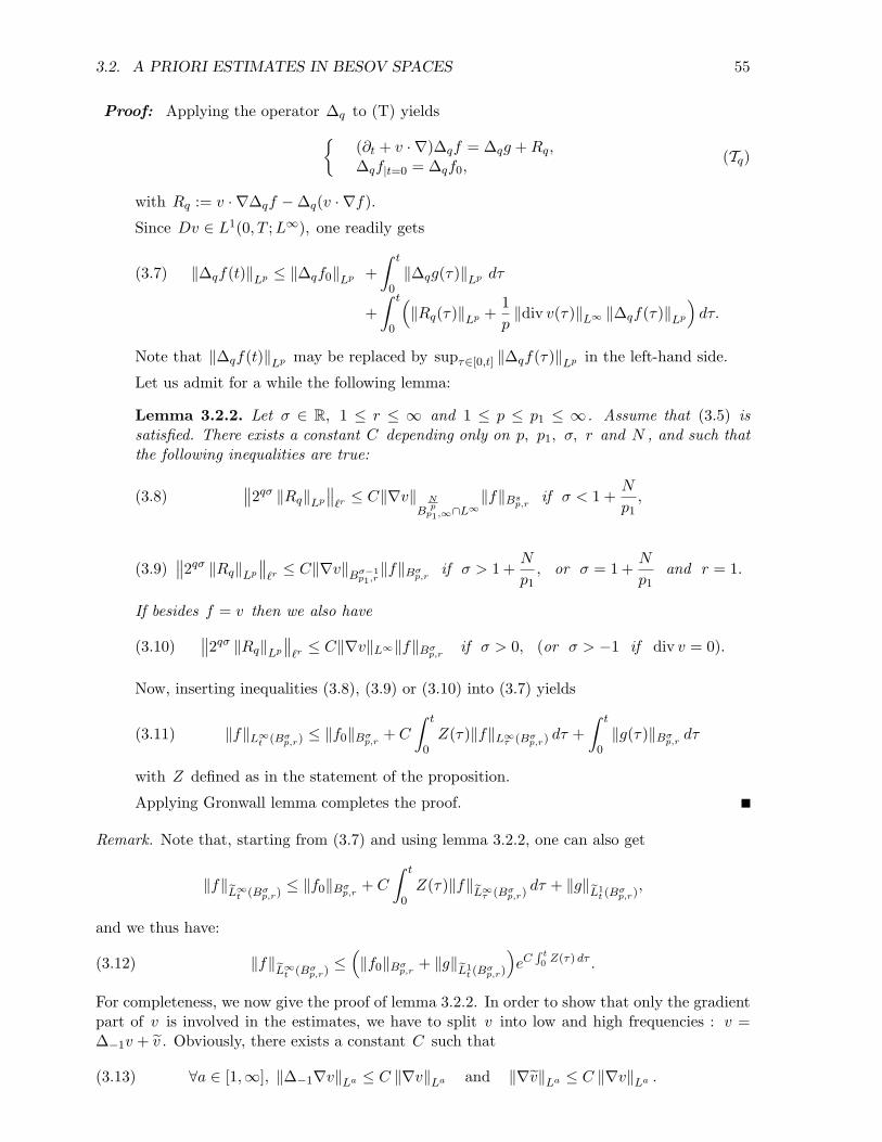
3.2. A PRIORI ESTIMATES IN BESOV SPACES 55

Proof: Applying the operator ∆q to (T) yields(∂t + v · ∇)∆qf = ∆qg +Rq,∆qf|t=0 = ∆qf0,

(Tq)

with Rq := v · ∇∆qf −∆q(v · ∇f).

Since Dv ∈ L1(0, T ;L∞), one readily gets

(3.7) ‖∆qf(t)‖Lp ≤ ‖∆qf0‖Lp +∫ t

0‖∆qg(τ)‖Lp dτ

+∫ t

0

(‖Rq(τ)‖Lp +

1p‖div v(τ)‖L∞ ‖∆qf(τ)‖Lp

)dτ.

Note that ‖∆qf(t)‖Lp may be replaced by supτ∈[0,t] ‖∆qf(τ)‖Lp in the left-hand side.

Let us admit for a while the following lemma:

Lemma 3.2.2. Let σ ∈ R, 1 ≤ r ≤ ∞ and 1 ≤ p ≤ p1 ≤ ∞. Assume that (3.5) issatisfied. There exists a constant C depending only on p, p1, σ, r and N , and such thatthe following inequalities are true:

(3.8)∥∥2qσ ‖Rq‖Lp

∥∥`r ≤ C‖∇v‖

BNp

p1,∞∩L∞‖f‖Bs

p,rif σ < 1 +

N

p1,

(3.9)∥∥2qσ ‖Rq‖Lp

∥∥`r ≤ C‖∇v‖Bσ−1

p1,r‖f‖Bσ

p,rif σ > 1 +

N

p1, or σ = 1 +

N

p1and r = 1.

If besides f = v then we also have

(3.10)∥∥2qσ ‖Rq‖Lp

∥∥`r ≤ C‖∇v‖L∞‖f‖Bσ

p,rif σ > 0, (or σ > −1 if div v = 0).

Now, inserting inequalities (3.8), (3.9) or (3.10) into (3.7) yields

(3.11) ‖f‖L∞t (Bσp,r) ≤ ‖f0‖Bσ

p,r+ C

∫ t

0Z(τ)‖f‖L∞τ (Bσ

p,r) dτ +∫ t

0‖g(τ)‖Bσ

p,rdτ

with Z defined as in the statement of the proposition.

Applying Gronwall lemma completes the proof.

Remark. Note that, starting from (3.7) and using lemma 3.2.2, one can also get

‖f‖eL∞t (Bσp,r)

≤ ‖f0‖Bσp,r

+ C

∫ t

0Z(τ)‖f‖eL∞τ (Bσ

p,r)dτ + ‖g‖eL1

t (Bσp,r),

and we thus have:

(3.12) ‖f‖eL∞t (Bσp,r)

≤(‖f0‖Bσ

p,r+ ‖g‖eL1

t (Bσp,r)

)eC

R t0 Z(τ) dτ .

For completeness, we now give the proof of lemma 3.2.2. In order to show that only the gradientpart of v is involved in the estimates, we have to split v into low and high frequencies : v =∆−1v + v . Obviously, there exists a constant C such that

(3.13) ∀a ∈ [1,∞], ‖∆−1∇v‖La ≤ C ‖∇v‖La and ‖∇v‖La ≤ C ‖∇v‖La .

56 CHAPTER 3. THE TRANSPORT EQUATION

Since there exists a R > 0 so that Supp F v ∩B(0, R) = ∅ , Bernstein lemma yields

(3.14) ∀a ∈ [1,∞], ∀q ≥ −1, ‖∆q∇v‖La ≈ 2q ‖∆qv‖La .

Now, we have (with the summation convention over repeated indices):

Rq = v · ∇∆qf −∆q(v · ∇f),= [vj ,∆q]∂jf + [∆−1v

j ,∆q]∂jf.

Hence, taking advantage of Bony’s decomposition, we end up with Rq =∑6

i=1Riq where

R1q = [Tevj ,∆q]∂jf,

R2q = T∂j∆qf v

j ,

R3q = −∆qT∂jf v

j ,

R4q = ∂jR(vj ,∆qf)− ∂j∆qR(vj , f),

R5q = ∆qR(div v, f)−R(div v,∆qf),

R6q = [∆−1v

j ,∆q]∂jf.

In the following computations, the constant C depends only on σ, p, p1, r and N and wedenote by (cq) a sequence such that ‖(cq)‖`r ≤ 1.

Bounds for 2qσ∥∥R1

q

∥∥Lp :

By virtue of proposition 1.2.1, we have

R1q =

∑|q−q′|≤4

[Sq′−1vj ,∆q]∂j∆q′f.

Using the definition of the operator ∆q leads to

[Sq′−1vj ,∆q]∂j∆q′f(x) =

∫h(y)

[Sq′−1v

j(x)− Sq′−1vj(x− 2−qy)

]∂j∆q′f(x− 2−qy) dy

so that applying first order Taylor’s formula, convolution inequalities and (3.13) yields

2qσ∥∥R1

q

∥∥Lp ≤ C ‖∇v‖L∞

∑|q′−q|≤4

2q′σ∥∥∆q′f

∥∥Lp ,

≤ Ccq ‖∇v‖L∞ ‖f‖Bσp,r.(3.15)

Bounds for 2qσ∥∥R2

q

∥∥Lp :

By virtue of proposition 1.2.1, we have

R2q =

∑q′≥q−3

Sq′−1∂j∆qf ∆q′ vj .

Hence, using inequalities (3.13) and (3.14) yields

(3.16) 2qσ∥∥R2

q

∥∥Lp ≤ Ccq ‖∇v‖L∞ ‖f‖Bσ

p,r.

3.2. A PRIORI ESTIMATES IN BESOV SPACES 57

Bounds for 2qσ∥∥R3

q

∥∥Lp :

One proceeds as follows :

R3q = −

∑|q′−q|≤4

∆q

(Sq′−1∂jf∆q′ v

j),(3.17)

= −∑

|q′−q|≤4q′′≤q′−2

∆q

(∆q′′∂jf∆q′ v

j).(3.18)

Therefore, denoting 1/p2 = 1/p− 1/p1 and taking advantage of (3.13) and (3.14),

2qσ∥∥R3

q

∥∥Lp ≤ C

∑|q′−q|≤4q′′≤q′−2

2qσ∥∥∆q′′∂jf

∥∥Lp2

∥∥∆q′ vj∥∥

Lp1,

≤ C∑

|q′−q|≤4q′′≤q′−2

2(q−q′′)(σ−1− Np1

)2q′′σ∥∥∆q′′f

∥∥Lp 2q′ N

p1

∥∥∆q′∇v∥∥

Lp1.

Hence, if σ < 1 +N/p1,

(3.19) 2qσ∥∥R3

q

∥∥Lp ≤ Ccq‖∇v‖

BNp1p1,∞

‖f‖Bσp,r.

Note that, starting from (3.17), one can alternately get

2qσ∥∥R3

q

∥∥Lp ≤ C

∑|q′−q|≤4

∥∥∇Sq′−1f∥∥

Lp22q′(σ−1)

∥∥∆q′∇v∥∥

Lp1.

As it may be proved that Bσ−1p,r → Lp2 in the cases σ > 1 +N/p1, or σ = 1 +N/p1 and r = 1,

we eventually get

(3.20) 2qσ∥∥R3

q

∥∥Lp ≤ Ccq‖∇v‖Bσ−1

p1,r‖f‖Bσ

p,r.

Bounds for 2qσ∥∥R4

q

∥∥Lp :

R4q =

∑|q′−q|≤2

∂j(∆q′ vj∆q∆q′f)

︸ ︷︷ ︸R4,1

q

−∑

q′≥q−3

∂j∆q(∆q′ vj∆q′f)︸ ︷︷ ︸

R4,2q

For the first term, we merely have (by virtue of (3.14)),

2qσ∥∥R4,1

q

∥∥Lp ≤ C ‖∇v‖L∞

∑|q′−q|≤2

2q′σ∥∥∥∆q′f

∥∥∥Lp,

whence

(3.21) 2qσ∥∥R4,1

q

∥∥Lp ≤ Ccq‖∇v‖L∞‖f‖Bσ

p,r.

For R4,2q , we proceed differently according to the value of 1/p+ 1/p1 . If 1/p + 1/p1 ≤ 1, we

define p2 by the relation 1/p2 := 1/p+1/p1. Then under condition σ > −1−N/p1, proposition

1.4.2 combined with the embedding Bσ+ N

p1p2,r → Bσ

p,r insures that we have

(3.22) 2qσ∥∥R4,2

q

∥∥Lp ≤ Ccq‖v‖

BNp1

+1

p1,∞

‖f‖Bσp,r.

Now, if 1/p + 1/p1 > 1, the above argument has to be applied with p′ instead of p2 and onestill ends up with (3.22) provided that σ > −1−N/p′.

Putting (3.21), (3.22) together and appealing to (3.13), one gets

(3.23) 2qσ∥∥R4

q

∥∥Lp ≤ Ccq‖∇v‖

BNp1p1,∞

‖f‖Bσp,r.

58 CHAPTER 3. THE TRANSPORT EQUATION

Bounds for 2qσ∥∥R5

q

∥∥Lp :

The arguments are the same as for R4q . Under condition σ > −N min(1/p1, 1/p′), one gets

(3.24) 2qσ∥∥R5

q

∥∥Lp ≤ Ccq‖∇v‖

BNp1p1,∞

‖f‖Bσp,r.

Bounds for 2qσ∥∥R6

q

∥∥Lp :

As R6q =

∑|q′−q|≤1[∆q,∆−1v] · ∇∆q′f, the first order Taylor formula yields

2qσ∥∥R6

q

∥∥Lp ≤ C

∑|q′−q|≤1

‖∇∆−1v‖L∞ 2q′σ∥∥∆q′f

∥∥Lp ,

≤ Ccq ‖∇v‖L∞ ‖f‖Bσp,r.(3.25)

Combining inequalities (3.15), (3.16), (3.19) or (3.20), (3.23), (3.24) and (3.25) yields (3.8) and(3.9). The proof of inequality (3.10) is left to the reader (see exercise (3.2)).

3.3 Solving the transport equation in Besov spaces

Let us now state our existence result for the transport equation with data in Besov spaces:

Theorem 3.3.1. Let p, p1, r and σ be as in the statement of proposition 3.2.1. Let f0 ∈ Bsp,r

and g ∈ L1(0, T ;Bsp,r). Let v be a time dependent vectorfield with coefficients in Lρ(0, T ;B−M

∞,∞)

for some ρ > 1 and M > 0, and such that Dv ∈ L1(0, T ;BNp1p1,∞ ∩ L∞) if σ < 1 +

N

p1, and

Dv ∈ L1(0, T ;Bσ−1p1,r ) if σ > 1+

N

p1or σ = 1+

N

p1and r = 1.

Then equation (T ) has a unique solution f ∈ L∞(0, T ;Bσp,r)⋂(

∩σ′<σC([0, T ];Bσ′p,1))

and theinequalities of proposition 3.2.1 hold true.

If moreover r is finite then we have f ∈ C([0, T ];Bσp,r).

Proof: Uniqueness readily stems from proposition 3.2.1 so let us tackle directly the proof ofthe existence. For the sake of conciseness, we treat only the case σ < 1 + N

p1.

We first smooth out the data and the velocity field v by setting

fn0 := Snf0, gn = ρn ∗t Sng and vn = ρn ∗t Snv

where ρn := ρn(t) stands for a sequence of mollifiers with respect to the time variable4.

We clearly have fn0 ∈ B∞

p,r, g ∈ C([0, T ];B∞p,r), v

n ∈ C([0, T ]×RN ) and Dvn ∈ C([0, T ];B∞p,r)

with B∞p,r :=

⋂s∈RB

sp,r. Moreover fn

0 is uniformly bounded in Bσp,r, g

n is uniformlybounded in L1(0, T ;Bσ

p,r), vn is uniformly bounded in Lρ(0, T ;B−M

∞,∞) and Dvn is uni-

formly bounded in L1(0, T ;BNp1p1,∞ ∩ L∞).

Let fn be the solution to

∂tfn + vn · ∇fn = gn, fn

|t=0 = fn0 .

Of course fn is smooth and, according to proposition 3.2.1, we have

(3.26) ‖fn(t)‖Bσp,r≤ eC

R t0 Zn(τ) dτ

(‖fn

0 ‖Bσp,r

+∫ t

0e−C

R τ0 Zn(τ ′) dτ ′‖fn(τ)‖Bσ

p,rdτ

)4with no loss of generality, one can assume that v and g are defined on R× RN .

3.3. SOLVING THE TRANSPORT EQUATION IN BESOV SPACES 59

with Zn(t) := ‖∇vn(t)‖B

Np1p1,∞∩L∞

.

Thus, according to the uniform bounds for fn0 , g

n and vn, one can conclude that sequence(fn)n∈N is uniformly bounded in C([0, T ];Bσ

p,r).

There are several ways to prove the convergence of (fn)n∈N, all of them being quitecumbersome if written into details. For instance, one can show that (fn)n∈N is a Cauchysequence in C([0, T ];Bσ−1

p,r ) (if σ is not too negative), or use a duality method or appealto compactness arguments.

In the present notes, we are going to use compactness. Let us first observe that (∂tfn −

gn)n∈N is uniformly bounded in Lα(0, T ;B−mp,∞) for some α > 1, and some m > 0. This

may be proved by observing that

(3.27) ∂tfn − gn = ∆−1v

n · ∇fn + (Id−∆−1)vn · ∇fn.

Indeed, because ∇fn is uniformly bounded in L∞(0, T ;Bs−1p,r ) and ∆−1v

n, uniformlybounded in Lρ(0, T ; C∞b ) (where C∞b stands for the set of smooth bounded functions withbounded derivatives5), the first term in the right-hand side of (3.27) is uniformly boundedin Lρ(0, T ;Bs−1

p,r ). Now, as for small enough ε the function (Id − ∆−1)vn is uniformly

bounded in Lα(0, T ;BNp1

+1−ε

p1+ε,r ) for some α > 1 (interpolate between the uniform bounds

in L1(0, T ;BNp1

+1

p1,∞ ) and in Lρ(0, T ;B−M∞,∞) for (Id−∆−1)vn ), one can conclude by appeal-

ing to propositions 1.4.1 and 1.4.2 that the last term in (3.27) is uniformly bounded inLα(0, T ;B−m

p,∞) for some large enough m > 0.

Integrating in time and denoting fn(t) := fn−∫ t0 g

n(τ) dτ, we thus gather that there existssome β > 0 such that the sequence (fn)n∈N is uniformly bounded in Cβ([0, T ];B−m

p,∞),hence uniformly equicontinuous with values in B−m

p,∞.

Next, assuming that m is large enough, proposition 1.4.6 guarantees that for all ϕ ∈ C∞cthe map u 7→ ϕu is compact from Bs

p,r to B−mp,∞. Combining Ascoli theorem and Cantor

diagonal process thus insures that, up to a subsequence, sequence (fn)n∈N converges inS ′ to some distribution f such that ϕf belongs to C([0, T ];B−m

p,∞) for all ϕ ∈ C∞c .

Finally, by taking advantage once again of the uniform bounds in L∞(0, T ;Bσp,r) and of the

Fatou property for Besov spaces, we get f ∈ L∞(0, T ;Bσp,r) and, by interpolation, better

results of convergence so that it becomes easy to check that the function f := f+∫ t0 g(τ) dτ

is a solution to (T ) (that the data fn0 , g

n and vn converge to f, g and v may be easilydeduced from their definition).

We still have to prove that f ∈ C([0, T ];Bσp,r) in the case where r is finite. Just by

looking at the equation (T), it is easy to get ∂tf ∈ L1(0, T ;B−M ′p,∞ ) for some large enough

M ′. Hence f belongs to C([0, T ];B−M ′p,∞ ). Therefore ∆qf ∈ C([0, T ];Lp) for any q ≥ −1,

whence Sqf ∈ C([0, T ];Bσp,r) for all q ∈ N .

We claim that the sequence of continuous Bsp,r valued functions (Sqf)q∈N converges uni-

formly on [0, T ]. Indeed, according to (1.1),

∆q′(f − Sqf) =∑

|q′′−q′|≥1q′′≥q

∆q′∆q′′f

5Here comes the assumption that v ∈ Lρ(0, T ;B−M∞,∞).

60 CHAPTER 3. THE TRANSPORT EQUATION

whence

(3.28) ‖f − Sqf‖Bσp,r≤ C

∑q′≥q−1

(2q′σ

∥∥∆q′f∥∥

Lp

)r

1r

.

Using inequality (3.7) to bound the right-hand side of (3.28), we gather

‖f − Sqf‖L∞T (Bσp,r) .

(( ∑q′≥q−1

(2q′σ

∥∥∆q′f0

∥∥Lp

)r) 1

r

+∫ T

0

( ∑q′≥q−1

(2q′σ

∥∥∆q′g(t)∥∥

Lp

)r) 1r

dt

+‖f‖L∞T (Bσp,r)

∫ T

0

( ∑q′≥q−1

cq′(t)r

) 1r

Z(t) dt

),

with∑

q′≥−1 cq′(t) ≤ 1 for all t ∈ [0, T ].

The first term clearly tends to zero when q tends to infinity. The terms in the integralsalso tend to zero for almost every t. Lebesgue dominated convergence theorem enables usto conclude that ‖f − Sqf‖L∞T (Bσ

p,r) tends to zero when q tends to infinity. This achievesto proving that u ∈ C([0, T ];Bσ

p,r) in the case r < +∞ .

When r = +∞ , we use that for any σ′ < σ we have the embedding Bσp,∞ → Bσ′

p,1 so thatthe above argument may be repeated in the space Bσ′

p,1 . This yields f ∈ C([0, T ];Bσ′p,1).

3.4 On the Cauchy problem for a shallow water equation

Let us first point out that theorem 3.3.1 is a good starting point for the study of general (possiblyN -dimensional) equations of the type

∂tu+ u · ∇u = f(u,∇u, · · · ),

including the incompressible Euler equation, provided the nonlinearity is of first order at most.In the present section, we show how it may be used to solve a nonlinear one-dimensional

shallow water equation which has been much studied recently: the so-called Camassa-Holmequation.

3.4.1 About Camassa-Holm equation

The one-dimensional model we are interested in reads:

(3.29) ∂tv − ∂3txxv + 2κ∂xv + 3v∂xv = 2∂xv∂

2xxv + v∂3

xxxv.

Above, the scalar function u = u(t, x) stands for the fluid velocity at time t ≥ 0 in the xdirection and κ is a non-negative parameter. For simplicity, we assume that x belongs to R.Similar results are true if x belongs to the circle, though.

Equation (3.29) has been derived independently by A. Fokas and B. Fuchssteiner in [27], andby R. Camassa and D. Holm in [6]. Its systematic mathematical study has been initiated in aseries of papers by A. Constantin and J. Escher (see e.g [16]).

We shall concentrate on the case κ = 0 (which actually is not restrictive since the change ofvariables u(t, x) = v(t, x−κt)+κ leads to (3.29) with κ = 0). It turns out that equation (3.29)with κ = 0 has many remarkable structural properties. In particular, it has infinitely manyconservation laws, the most obvious ones being the conservation of the average over R and ofthe H1 norm for smooth solutions with sufficient decay at infinity. By taking advantage of this

3.4. ON THE CAUCHY PROBLEM FOR A SHALLOW WATER EQUATION 61

latter property, Z. Xin and P. Zhang proved that (3.29) has global weak solutions for any datain H1 (see [39]).

In the present chapter, we address the question of existence and uniqueness for the initialvalue problem. For simplicity, we restrict ourselves to the evolution for positive times. Ofcourse, one would get similar results for negative times: this is just a matter of changing theinitial condition u0 into −u0 .

At this point, one can wonder which regularity assumptions are relevant for u0 so that theinitial value problem be well-posed in the sense of Hadamard (i.e. (CH) has a unique localsolution in a suitable functional setting, and continuity with respect to the initial data holdstrue).

In order to go further into the quest for a good functional framework, let us observe thatone can get rid very easily of the third order terms. Indeed: applying the pseudo-differentialoperator (1− ∂2

x)−1 to (3.29), we discover that (CH) is equivalent to

(CH)∂tu+ u∂xu = P (D)

(u2 + 1

2(∂xu)2),

u|t=0 = u0,

with P (D) = −∂x(1− ∂2x)−1 .

Hence Camassa-Holm equation is nothing but a generalized Burgers equation with a nonlo-cal nonlinearity of order 0. In light of proposition 3.3.1, we can thus expect that a necessarycondition for well-posedness for data in some functional space E is that E be embedded in thespace Lip of continuous bounded functions with bounded derivatives.

Moreover, as the solution u is expected to be only in C([0, T ];E) (a gain of regularity cannotbe expected in a Burgers like equation), the application

G : u 7→ P (D)(u2 + 1

2(∂xu)2)

must map E to E continuously.

3.4.2 A well-posedness result and a blow-up criterion

If we restrict ourselves to the framework of nonhomogeneous Besov space Bsp,r, the condition

E ⊂ Lip is equivalent to s > 1 + 1/p (or s ≥ 1 + 1/p if r = 1), and no further restrictionsare needed for the continuity of the map G (up to the endpoint r = 1, s = 1, p = +∞ whichhas to be avoided). We shall see however that for proving uniqueness, our method requiresthat in addition we have s > max(1 + 1/p, 3/2). Let us mention in passing that in the periodicframework, by using the Lagrangian formulation for Camassa-Holm equation, it is actuallypossible to weaken the condition on s (see [26]).

For stating our local existence result, the following functional spaces are needed:

Esp,r(T ) := C([0, T ];Bs

p,r) ∩ C1([0, T ];Bs−1p,r ) if r <∞,

Esp,∞(T ) := L∞(0, T ;Bs

p,∞) ∩ Lip([0, T ];Bs−1p,∞)

with T > 0, s ∈ R and 1 ≤ p, r ≤ ∞.

Theorem 3.4.1. Let 1 ≤ p, r ≤ ∞ and s > max(3/2, 1 + 1/p). Let u0 ∈ Bsp,r. There exists a

time T > 0 such that (CH) has a unique solution u in Esp,r(T ).

We can also state a result of conservation of energy for smooth solutions:

Theorem 3.4.2. Let s, p, r be as in theorem 3.4.1. Let u ∈ Esp,r(T ) be a solution of (CH) on

[0, T ]× R with data u0 ∈ Bsp,r ∩H1. Then the solution u to (CH) satisfies

(3.30) ∀t ∈ [0, T ], ‖u(t)‖H1 = ‖u0‖H1 .

62 CHAPTER 3. THE TRANSPORT EQUATION

Before stating blow-up criteria, let us give the definition of the lifespan of solutions withdata in Bs

p,r.

Definition. Let u0 ∈ Bsp,r . We define the lifespan T ?

u0of the solutions of (CH) with initial

data u0 as the supremum of positive times T such that (CH) has a solution u ∈ Esp,r(T ) on

[0, T ]× R.

Our main blow-up criterion reads:

Theorem 3.4.3. Let u0 be as in theorem 3.4.1 and u be the corresponding solution. Then

T ?u0<∞ =⇒

∫ T ?u0

0‖∂xu(τ)‖L∞ dτ = ∞.

3.4.3 Uniqueness

Let us start this section with a lemma:

Lemma 3.4.4. Let 1 ≤ p, r ≤ ∞, and (σ1, σ2) ∈ R2 be such that

Bσ2p,r → Lip, σ1 ≤ σ2 and σ1 + σ2 > 2 + max

(0,

2p− 1).

Then the function B : (f, g) 7→ P (D)(fg + 1

2∂xf ∂xg)

maps Bσ1p,r ×Bσ2

p,r in Bσ1p,r.

Proof: We notice that P (D) is a multiplier of degree −1. Hence, according to proposition1.3.7, it suffices to prove that the functional

H : (f, g) 7→ fg + 12∂xf ∂xg

maps Bσ1p,r ×Bσ2

p,r in Bσ1−1p,r .

The term fg is easy to handle so we focus on the study of ∂xf∂xg. By virtue of Bony’sdecomposition, we have

∂xf∂xg = T∂xf∂xg + T∂xg∂xf +R(∂xf, ∂xg).

Proposition 1.4.1 insures that the application (f, g) 7→ T∂xf∂xg is continuous from Bσ1p,r ×

Bσ2p,r to

• the space Bσ1+σ2−2− 1

pp,r if σ1 < 1 + 1

p ,

• the space Bσ2−1−εp,r for all ε > 0, if σ1 = 1 + 1

p and r > 1,

• the space Bσ2−1p,r if σ1 = 1 + 1

p and r = 1, or σ1 > 1 + 1p .

According to our assumptions on σ1, σ2, p and r, we thus can conclude that (f, g) 7→T∂xf∂xg maps Bσ1

p,r ×Bσ2p,r in Bσ1−1

p,r .

Since Bσ2−1p,r → L∞, proposition 1.4.1 readily yields the continuity of (f, g) 7→ T∂xg∂xf

from Bσ1p,r ×Bσ2

p,r to Bσ1−1p,r .

Finally, the remainder term maps Bσ1p,r×Bσ2

p,r in Bσ1+σ2−2− 1

pp,r (and thus in Bσ1−1

p,r ) providedthat σ1 + σ2 > 2 + max

(0, 2

p − 1).

Uniqueness in theorem 3.4.1 is a straightforward corollary of the following proposition.

3.4. ON THE CAUCHY PROBLEM FOR A SHALLOW WATER EQUATION 63

Proposition 3.4.5. Let 1 ≤ p, r ≤ +∞ and s > max(1 + 1/p, 3/2). Suppose that we are given(u, v) ∈

(L∞(0, T ;Bs

p,r) ∩ C([0, T ];Bs−1p,r )

)2 two solutions of (CH) with initial data u0, v0 ∈ Bsp,r .

Then we have for every t ∈ [0, T ]:

‖u(t)− v(t)‖Bs−1p,r

≤ ‖u0 − v0‖Bs−1p,r

eC

R t0

(‖u(τ)‖Bs

p,r+‖v(τ)‖Bs

p,r

)dτ.

Proof: It is obvious that w := v − u solves the transport equation:

∂tw + u∂xw = −w∂xv + P (D)(w(u+v) + 1

2∂xw ∂x(u+v)).

According to propositions 3.2.1 and 1.3.7, the following inequality holds true:

(3.31) ‖w(t)‖Bs−1p,r

≤ ‖w0‖Bs−1p,r

eC

R t0 ‖∂xu‖

Bs−1p,r

dτ ′

+ C

∫ t

0eC

R tτ ‖∂xu‖

Bs−1p,r

dτ ′

×(‖w∂xv‖Bs−1

p,r+ ‖B(w, u+v)‖Bs−1

p,r

)dτ,

where B stands for the symmetric bilinear function introduced in lemma 3.4.4.

Since s > max(32 , 1 + 1

p), we thus have

‖B(w, u+v)‖Bs−1p,r

≤ C‖w‖Bs−1p,r

(‖u‖Bs

p,r+ ‖v‖Bs

p,r

).

Plugging this last inequality in (3.31) and applying Gronwall lemma completes the proof.

Remark. For proving uniqueness, we are led to estimate in Bs−1p,r the difference between two

solutions although both solutions are in Bsp,r. Owing to the term (∂xu)2, the additional condition

s > max(32 , 1 + 1

p) is thus required. In fact, uniqueness is also in true in B322,1, see [24]. It

has been discovered recently in [26] that if using the Lagrangian formulation, one can directlyprove uniqueness in a space with the regularity index s and forget about the restriction s >max(3

2 , 1 + 1p).

3.4.4 The proof of existence

Let us first enumerate the main steps of the proof of theorem 3.4.1.

(i) Construction of approximate solutions of (CH) which are smooth solutions of some lineartransport equation.

(ii) Find a positive T for which these approximate solutions are uniformly bounded in Esp,r(T ).

(iii) Prove that the sequence of approximate solutions is a Cauchy sequence in a larger space.

(iv) Check that the limit has indeed the required regularity.

First step: approximate solution

We use a standard iterative process to build a solution. Starting from u0 := 0, we then defineby induction a sequence of smooth functions (un)n∈N by solving the following linear transportequation:

(Tn)

(∂t + un∂x)un+1 = P (D)

((un)2 + 1

2(∂xun)2),

un+1|t=0 = un+1

0 := Sn+1 ? u0.

Since all the data belong to B∞p,r, theorem 3.3.1 enables us to show by induction that for all

n ∈ N, the above equation has a global solution which belongs to C(R+;B∞p,r).

64 CHAPTER 3. THE TRANSPORT EQUATION

Second step: uniform bounds

According to theorem 3.3.1 and to lemma 3.4.4, we have the following inequality for all n ∈ N :

(3.32) ‖un+1(t)‖Bsp,r≤ CeCUn(t)

(‖u0‖Bs

p,r+∫ t

0e−CUn(τ)‖un(τ)‖2

Bsp,rdτ

)

with Un :=∫ t

0‖un(τ)‖Bs

p,rdτ.

Let us fix a T > 0 such that 2C2‖u0‖Bsp,rT < 1 and suppose that

(3.33) ∀t ∈ [0, T ], ‖un(t)‖Bsp,r≤

C‖u0‖Bsp,r

1− 2C2‖u0‖Bsp,rt·

Plugging (3.33) in (3.32) yields

‖un+1(t)‖Bsp,r

≤ 1q1−2C2‖u0‖Bs

p,rt

(‖u0‖Bs

p,r+ C2‖u0‖2

Bsp,r

∫ t0

dτ

(1−2C2‖u0‖Bsp,r

τ)32

),

≤C‖u0‖Bs

p,r

1−2C2‖u0‖Bsp,r

t·

Therefore, (un)n∈N is uniformly bounded in C([0, T ];Bsp,r). This clearly entails that un∂xu

n

is uniformly bounded in C([0, T ];Bs−1p,r ). As the right-hand side of (Tn) has been shown to be

uniformly bounded in C([0, T ];Bsp,r), one can conclude that the sequence (un)n∈N is uniformly

bounded in Esp,r(T ).

Third step: convergence

We are going to show that (un)n∈N is a Cauchy sequence in C([0, T ];Bs−1p,r ).

We remark that for all (m,n) ∈ N2, we have

(∂t + un+m∂x)(un+m+1−un+1) = (un − un+m)∂xun+1 +B(un+m−un, un+m+un).

Applying theorem 3.3.1 and lemma 3.4.4, and using that Bs−1p,r is an algebra yields

∀t ∈ [0, T ], ‖(un+m+1−un+1)(t)‖Bs−1p,r

≤ eCUn+m(t)

(‖un+m+1

0 − un+10 ‖Bs−1

p,r

+C∫ t

0e−CUn+m(τ)‖un+m − un‖Bs−1

p,r

(‖un‖Bs

p,r+ ‖un+1‖Bs

p,r+ ‖un+m‖Bs

p,r

)dτ

).

Since (un)n∈N is uniformly bounded in Esp,r(T ) and

un+m+10 − un+1

0 =n+m+1∑q=n+2

∆qu0,

we finally get a constant CT independent of n,m and such that for all t ∈ [0, T ], we have

‖(un+m+1 − un+1)(t)‖Bs−1p,r

≤ CT

(2−n +

∫ t

0‖(un+m − un)(τ)‖Bs−1

p,rdτ

).

Arguing by induction, one can easily prove that

‖un+m+1 − un+1‖L∞T (Bs−1p,r ) ≤

(TCT )n+1

(n+ 1)!‖um‖L∞T (Bs

p,r) + CT

n∑k=0

2−(n−k) (TCT )k

k!.

3.4. ON THE CAUCHY PROBLEM FOR A SHALLOW WATER EQUATION 65

As ‖um‖L∞T (Bsp,r) may be bounded independently of m, we can conclude to the existence of some

new constant C ′T such that

‖un+m+1 − un+1‖L∞T (Bs−1p,r ) ≤ C ′T 2−n.

Hence (un)n∈N is a Cauchy sequence in C([0, T ];Bs−1p,r ), whence it converges to some limit

function u ∈ C([0, T ];Bs−1p,r ).

last step: conclusion

We now have to check that u belongs to Esp,r(T ) and satisfies (CH). Since (un)n∈N is uniformly

bounded in L∞(0, T ;Bsp,r), Fatou property for Besov spaces guarantees that u also belongs to

L∞(0, T ;Bsp,r).

On the other hand, as (un)n∈N converges to u in C([0, T ];Bs−1p,r ), an interpolation argument

insures that convergence actually holds true in C([0, T ];Bs′p,r) for any s′ < s. It is then easy to

pass to the limit in (Tn) and to conclude that u is indeed a solution to (CH).Now, because u belongs to L∞(0, T ;Bs

p,r), the right-hand side of the equation

∂tu+ u∂xu = P (D)(u2 + 12(∂xu)2)

also belongs to L∞(0, T ;Bsp,r). In the case r < ∞, theorem 3.3.1 enables us to conclude that

u ∈ C([0, T ];Bsp,r). Finally, using again the equation, we see that ∂tu is in C([0, T ];Bs−1

p,r ) if ris finite, and in L∞(0, T ;Bs−1

p,r ) otherwise. So finally, u belongs to Esp,r(T ).

Remark. If v0 is in a small neighborhood of u0 in Bsp,r , the arguments above give the existence

of a solution v ∈ Esp,r(T ) to (CH) with initial datum v0 . Proposition 3.4.5 combined with

an obvious interpolation ensures continuity with respect to the initial data in C([0, T ];Bs′p,r) ∩

C1([0, T ];Bs′−1p,r ) for any s′ < s .

The fact that continuity also holds in C([0, T ];Bsp,r) ∩ C1([0, T ];Bs−1

p,r ) when r < +∞ isnot obvious but belongs to the mathematical folklore. It may be proved through the use of asequence of approximate solutions (uε)ε>0 for (CH) which converges uniformly in C([0, T ];Bs

p,r)∩C1([0, T ];Bs−1

p,r ). A viscosity approximation gives the desired property of convergence.

3.4.5 Blow-up criterion and energy conservation

This section is devoted to the proof of theorems 3.4.3 and 3.4.2. Both theorems are based onthe following lemma:

Lemma 3.4.6. Let 1 ≤ p, r ≤ ∞ and s > 1. Let u ∈ L∞(0, T ;Bsp,r) solving (CH) on [0, T )×R

with u0 ∈ Bsp,r as an initial datum. There exist a constant C depending only on s and p, and

a universal constant C ′ such that for all t ∈ [0, T ), we have

‖u(t)‖Bsp,r

≤ ‖u0‖Bsp,reC

R t0 ‖u(τ)‖Lip dτ ,(3.34)

‖u(t)‖Lip ≤ ‖u0‖LipeC′ R t

0 ‖∂xu(τ)‖L∞ dτ .(3.35)

Proof: Applying the last part of proposition 3.2.1 to (CH) and using the fact that P (D) isa multiplier of order −1 yields

e−CR t0 ‖∂xu‖L∞ dτ‖u(t)‖Bs

p,r≤ ‖u0‖Bs

p,r+C

∫ t

0e−C

R τ0 ‖∂xu‖L∞ dτ ′

(‖u2‖Bs−1

p,r+‖(∂xu)2‖Bs−1

p,r

)dτ.

As s− 1 > 0, we have, according to proposition 1.4.3,

‖u2‖Bs−1p,r

+ ‖(∂xu)2‖Bs−1p,r

≤ C‖u‖Lip‖u‖Bsp,r.

66 CHAPTER 3. THE TRANSPORT EQUATION

Therefore

e−CR t0 ‖∂xu‖L∞ dτ‖u(t)‖Bs

p,r≤ ‖u0‖Bs

p,r+ C

∫ t

0e−C

R τ0 ‖∂xu‖L∞ dτ ′‖u‖Bs

p,r‖u‖Lip dτ.

Applying Gronwall lemma completes the proof of (3.34).

By differentiating once equation (CH) with respect to x, and applying the L∞ estimatefor transport equations, we easily prove that

e−R t0 ‖∂xu‖L∞ dτ‖u(t)‖Lip ≤ ‖u0‖Lip +

∫ t

0e−

R τ0 ‖∂xu‖L∞ dτ ‖P (D)

(u2 + 1

2(∂xu)2)‖Lip.

Now, exercise 3.3 guarantees that

‖P (D)(u2 + 1

2(∂xu)2)‖Lip ≤ C ′‖u‖Lip ‖∂xu‖L∞

for some universal constant C ′. Hence Gronwall lemma gives inequality (3.35).

We can now prove theorem 3.4.3. Let u ∈⋂

T<T ? Esp,r(T ) be such that

∫ T ?

0 ‖∂xu(τ)‖L∞ dτ befinite. According to inequality (3.35),

∫ T ?

0 ‖u(τ)‖Lip dτ is also finite. Hence, (3.34) insures that

(3.36) ∀t ∈ [0, T ?), ‖u(t)‖Bsp,r≤MT ? := ‖u0‖Bs

p,reC

R T?

0 ‖u(τ)‖Lip dτ <∞.

Let ε > 0 be such that 2C2εMT ? < 1 where C stands for the constant used in the proof oftheorem 3.3.1. We then have a solution u ∈ Es

p,r(ε) to (CH) with initial datum u(T ?−ε/2).For the sake of uniqueness, u(t) = u(t+ T ? − ε/2) on [0, ε/2) so that u extends the solution ubeyond T ? . We conclude that T ? < T ?

u0and theorem 3.4.3 is proved.

Let us now prove theorem 3.4.2. Assume that u0 belongs to H1∩Bsp,r with s > max(3/2, 1+

1/p), and that the corresponding solution u is defined on [0, T ] and belongs to Esp,r(T ). We

want to prove that the H1 norm of u is conserved. Clearly, this cannot be done by using theapproximation scheme of theorem 2.7 since it does not conserve the H1 norm.

An alternative method is to mollify the initial datum u0 and to define un as the maximalsolution of (CH) corresponding to un

0 then pass to the limit. This time, we set un0 := ρn ? u0

where (ρn)n∈N stands for a sequence of nonnegative mollifiers.Owing to the nonnegativity of the mollifiers, one can easily check that

‖un0‖Bs

p,r≤ ‖u0‖Bs

p,rand ‖un

0‖H1 ≤ ‖u0‖H1 .

Following the second step of the proof of theorem 3.4.1, we discover that there exists a constantC such that un is a solution of (CH) on [0, T ]× R with

T := C/‖u‖L∞T (Bsp,r)

and un ∈ Esp,r(T ) uniformly.

Now, we also have un0 ∈ H4 so that, there exists some Tn > 0 such that (CH) with data

un0 has a solution un ∈ C([0, Tn];H4). By virtue of uniqueness, we actually have un ≡ un on

[0,min(T , Tn)], and according to lemma (3.4.6) and to Besov embeddings,

∀t ∈ [0,min(T , Tn)], ‖un(t)‖H4 ≤ ‖un0‖H4e

CR t0 ‖u

n(τ)‖Bsp,r

dτ.

Note that the right-hand side may be bounded independently of n and of t ∈ [0, T ]. Therefore,arguing as in the proof of the first part of theorem 3.4.3, one can conclude that Tn may bechosen greater than T .

3.4. ON THE CAUCHY PROBLEM FOR A SHALLOW WATER EQUATION 67

Now, the smoothness of un enables us to derive directly from (3.29) that

(3.37) ∀t ∈ [0, T ], ‖un(t)‖H1 = ‖un0‖H1 ≤ ‖u0‖H1 .

Therefore, passing to the limit (use e.g. proposition 3.4.5) and using Fatou property for H1,one eventually gets ‖u(t)‖H1 ≤ ‖u0‖H1 for t ∈ [0, T ].

For proving the reverse inequality, one can solve the equation backward, starting from u(T ).Then, arguing as above and using uniqueness, one can assert that ‖u(T − t)‖H1 ≤ ‖u(T )‖H1 fort ≤ C/‖u‖L∞

T(Bs

p,r). Repeating the argument several times, we finally get ‖u(t)‖H1 = ‖u0‖H1 forall t ∈ [0, T ].

It is now easy to get equality on [0, T ]. Indeed, arguing as above yields equality on [T , 2T ],[2T , 3T ], etc. until the whole interval [0, T ] is exhausted.

Let us end this chapter with the statement of a slightly weaker blow-up criterion in the spiritof the celebrated Beale-Kato-Majda criterion for Euler equations (see for example [3] or [10]):

Proposition 3.4.7. Under the assumption that u0 ∈ Bsp,r with s > max(3/2, 1+1/p), we have:

(3.38) T ?u0< +∞ =⇒

∫ T ?u0

0‖u(τ)‖B1

∞,∞dτ = +∞.

Proof: This merely stems from the following logarithmic interpolation inequality:

‖u‖Lip ≤ C(1 + ‖u‖B1

∞,∞log(e+ ‖u‖Bs

p,r

)which holds true whenever s > 1 + 1/p and may be deduced from proposition 1.3.6 and

the embeddings B1∞,1 ∩ L∞ → Lip and Bs−1

p,1 → Bs−1− 1

p∞,∞ .

Plugging it into (3.36), we get

‖u(t)‖Bsp,r≤ ‖u0‖Bs

p,reCte

CR t0 ‖u‖B1∞,∞

log(e+‖u‖Bsp,r

) dτ.

Therefore, easy calculations lead to

log(e+ ‖u(t)‖Bs

p,r

)≤ log

(e+ ‖u0‖Bs

p,r

)+ Ct+ C

∫ t

0‖u‖B1

∞,∞log(e+ ‖u‖Bs

p,r

)dτ.

Gronwall lemma thus yields

log(e+ ‖u(t)‖Bs

p,r

)≤(log(e+ ‖u0‖Bs

p,r

)+ Ct

)eC

R t0 ‖u‖B1∞,∞

dτ.

One can now conclude that if∫ T0 ‖u‖B1

∞,∞dt <∞ then u ∈ L∞(0, T ;Bs

p,r). Arguing as intheorem 3.4.3 completes the proof of the proposition.

Remark. The fact that ‖∂xu(t)‖L∞ may be replaced with the weaker norm ‖∂xu(t)‖B0∞,∞

isactually not very sensitive to the structure of the equation. As pointed out above, a similarcriterion may be stated (with the same method) for the incompressible Euler equations, andalso for a number of quasilinear first order equations.We want to conclude this section with a more precise blow-up statement which is specific to theCamassa-Holm equation:

Proposition 3.4.8. Under the assumption that u0 ∈ Bsp,r ∩H1 with s > max(3/2, 1+1/p), we

have:

(3.39) T ?u0< +∞ =⇒

∫ T ?u0

0infx∈R

u(τ, x) dτ = −∞.

Proof: The reader is referred to [18].

68 CHAPTER 3. THE TRANSPORT EQUATION

3.5 Exercises

Exercise 3.1. Let v : R×RN → RN be a smooth time-dependent vectorfield, globally Lipschitzwith respect to the space variable, and ψt,s, the flow of v.

1) Check that ψt,s is defined for all (t, s) ∈ R2.

2) Prove that ∀(t, s) ∈ R2, ∀x ∈ RN , detDψt,s(x) = exp(∫ t

sdiv v(τ, ψτ,s(x)) dτ

).

3) Prove inequality (3.4) for smooth solutions which belong to L∞(0, T ;Lp).

4) Prove estimates in W 1,p spaces for the solutions to the transport equation (T).

Exercise 3.2. Prove inequality (3.10).

Exercise 3.3. Throughout the exercise, the function u is defined over R.

1) Prove that (1− ∂2xx)−1u = 1

2 e− |·| ∗ u.

2) From the first question, deduce that∥∥(1−∂2xx)−1u

∥∥L∞

≤ ‖u‖L∞ ,∥∥(1−∂2

xx)−1∂xu∥∥

L∞≤ ‖u‖L∞ ,∥∥(1−∂2

xx)−1∂x(u2)∥∥

L∞≤ 2 ‖u‖L∞ ‖∂xu‖L∞ ,

∥∥(1−∂2xx)−1∂2

xx(u2)∥∥

L∞≤ 2 ‖u‖L∞ ‖∂xu‖L∞ .

3) Let P (D) := ∂x(1− ∂2xx)−1. Prove the existence of a universal constant C such that

‖P (D)(u2 + 1

2(∂xu)2)‖Lip ≤ C‖u‖Lip ‖∂xu‖L∞ .

Chapter 4

A short insight into compressiblefluid mechanics

4.1 About the model

We first briefly explain how the system of equations for the flow of compressible fluids may bederived from basic physics.

4.1.1 Physical conservation laws

We assume that the fluid under consideration fills in a time independent open domain D of RN

and may be characterized for every material point x ∈ D at time t ∈ R, by

• its velocity field u := u(t, x),

• its density ρ := ρ(t, x),

• its internal energy e := e(t, x),

• its entropy by unit mass s := s(t, x).

For each subdomain Ω of D, one can define the following physical quantities:

• the mass: M(Ω) :=∫Ω ρ dx.

• the momentum: P (Ω) :=∫Ω ρu dx.

• the energy: E(Ω) :=∫Ω

(12ρ|u|

2 + ρe)dx.

• the entropy: S(Ω) :=∫Ω ρs dx.

Denoting by ψt the flow1 of u and Ωt := ψt(Ω), and assuming that there is no productionor loss of mass, we have the following conservation law:

(4.1)d

dtM(Ωt) =

d

dt

∫Ωt

ρ dx = 0.

For the momentum, we have

(4.2)d

dtP (Ωt) =

d

dt

∫Ωt

ρu dx =∫

Ωt

ρf dx+∫

∂Ωt

(σ · n) dΣ

1See the definition in chapter 3.

69

70 CHAPTER 4. A SHORT INSIGHT INTO COMPRESSIBLE FLUID MECHANICS

where the first term on the right-hand side represents external volume forces with density f(such as gravity for instance) and the second term, surface forces.

In the full generality, the strain about x ∈ ∂Ωt is some vector valued function T dependingon t, x and on the unit exterior normal vector n at x. Under the assumption of small strains,this function may be linearized so that it reduces to T (t, x, n) = σ(t, x) · n for some straintensor σ. In the absence of mass couples, an assumption that we are going to do from now on,the angular momentum

∫Ωtx ∧ (ρu)(t, x) dx is also conserved and one can prove that σ is a

symmetric tensor.

As regards the energy conservation, we have

(4.3)d

dtE(Ωt) =

d

dt

∫Ωt

ρ(e+

|u|2

2

)dx =

∫Ωt

ρf ·u dx+∫

∂Ωt

(σ ·n)·ndΣ−∫

∂Ωt

q ·ndΣ

where q is the heat flux vector.Finally, introducing the temperature T, the entropy balance writes:

(4.4)d

dtS(Ωt) =

d

dt

∫Ωt

ρs dx ≥ −∫

∂Ωt

(q · nT

)dΣ.

4.1.2 The full model

From the global conservation laws (4.1), (4.2), (4.3) and (4.4), one can obtain a system of PDE’sinvolving ρ, u, e, and s. This is a mere consequence of the following (formal) lemma.

Lemma 4.1.1. Let Ω be an open subdomain of D, ψ be the flow of u and Ωt := ψt(Ω). Thefollowing equalities hold true for all scalar function b:

d

dt

∫Ωt

b dx =∫

Ωt

(∂tb+ div bu

)dx,

=∫

Ωt

∂tb dx+∫

∂Ωt

(b u · n) dΣ.

Combining lemma 4.1.1 with relations (4.1), (4.2), (4.3) and (4.4), we obtain the followingequations for the evolution of compressible flows:

∂tρ+ div(ρu) = 0,(4.5)

∂tρu+ div(ρu⊗ u) = ρf + div σ,(4.6)

∂t

(ρ(e+

|u|2

2

))+ div

(ρ(e+

|u|2

2

)u

)= ρf · u+ div(σ · u)− div q,(4.7)

∂tρs+ div(ρsu) ≥ −div( qT

).(4.8)

From a mathematical viewpoint, the above equations are too general to be handled. In the nextsection, we shall restrict ourselves to particular fluids.

4.1.3 Simplifying assumptions

We shall first assume that the fluid is Newtonian, namely

• the tensor σ is a linear function of Du, invariant under rigid transforms,

• the fluid is isotropic (i.e the physical quantities depend only on (t, x)).

4.1. ABOUT THE MODEL 71

As a consequence, it may be shown that σ has the following form:

σ = (λ div u− p)Id + 2µD(u)

where the scalar function p = p(t, x) is the pressure, λ and µ are the viscosity coefficients andD(u) := 1

2(Du + tDu) is the deformation tensor. One can also introduce the viscous stresstensor :

τ := λ div u Id + 2µD(u).

Finally, we shall assume that Fourier law is satisfied, namely q = −k∇T.In full generality, the coefficients k, λ and µ may depend on ρ and T. For the sake of

simplicity however, we shall assume from now on that they are constant functions. We thusobtain the following system of equations:

∂tρ+ div(ρu) = 0,(4.9)

∂tρu+ div(ρu⊗ u)− µ∆u− (λ+ µ)∇ div u+∇p = ρf,(4.10)

∂t

(ρ(e+ |u|2

2

))+ div

(ρ(e+ |u|2

2

)u)

+ div pu− k∆T = ρf · u+ div(τ · u)− div q,(4.11)

∂tρs+ div(ρsu) ≥ k div(∇TT

).(4.12)

In dimension N, the above system has N +2 equations (and an inequation) for N +5 unknownscalar functions (namely ρ, u1, · · · , uN , p, e, T and s). In order to close the system, threeadditional equations are needed. As regards the entropy s, we assume that the so-called Gibbsrelation is satisfied:

Tds = de+ p d(1ρ

).

We still need two other equalities (often called state relations) involving p, ρ, e, s and T. Onecan assume for example that p = P (ρ, T ) and e = ε(ρ, T ) for some given functions P and εwhich may be determined from further physical considerations depending on the nature of thefluid. Combining Gibbs relation with the mass, momentum and energy equations, we get

∂tρs+ div(ρsu) = k div(∇TT

)+τ : D(u)

T+ k

|∇T |2

T 2·

Hence, according to the entropy inequality, we must have

τ : D(u) + k|∇T |2

T≥ 0.

This yields the following additional constraints on λ, µ and k :

(4.13) k ≥ 0, µ ≥ 0 and 2µ+Nλ ≥ 0.

Let us give some important examples:

• Monoatomic gases in dimension N = 3 satisfy 2µ + 3λ = 0. For more general fluids,2µ+ 3λ may be positive.

• Inviscid fluids are such that µ = λ = 0.

• By definition, a non conducting fluid is such that k = 0.

72 CHAPTER 4. A SHORT INSIGHT INTO COMPRESSIBLE FLUID MECHANICS

4.1.4 Barotropic fluids

From now, we shall consider a simplified model for compressible fluids, the so-called barotropicNavier-Stokes equations:

(4.14)∂tρ+ div ρ = 0,∂tρu+ div(ρu⊗ u)− µ∆u− (λ+ µ)∇ div u+∇p = ρf

with p = P (ρ) for some suitably smooth function P.

The above system may be derived from the general model (4.10), (4.11), (4.12) under theassumption that s is a constant and that the fluid is non conducting. Note that in the viscouscase (that we are going to consider in the next sections) the assumption of constant entropy issomewhat inconsistent with physics since the term τ : D(u) appearing in the entropy balancemay be positive. As a matter of fact, it turns out that, from a mathematical viewpoint, thebarotropic (or isentropic) model keeps most of the features of the full model.

4.2 Local well-posedness in critical spaces

From now on, we restrict ourselves to viscous fluids (i.e µ > 0) and we further assume (for thesake of simplicity only) that λ+µ = 02. We focus on flows whose density is a small perturbationof a positive constant, say 1 to simplify the notation.

Denoting a = ρ−1, the barotropic system for smooth enough solutions with positive densitythus reduces to

(NSC)

∂ta+ u · ∇a+ (1 + a) div u = 0,

∂tu− µ1+a∆u+ u · ∇u+∇g = f,

where g = G(a) stands for the chemical potential expressed in term of a. The function G isassumed to be conveniently smooth and, with no loss of generality, vanishes at 0.

The conducting thread for finding an appropriate framework is the same as in the incom-pressible case (see chapter 2): using functional spaces which have the same scaling invariance asthe system, if any.

For the velocity, one can expect the functional framework to be the same as the one usedin chapter 2. Now, one can notice that (NSC) is invariant for all λ > 0 by the rescaling(a, u) 7→ (aλ, uλ) with

aλ(t, x) = a(λ2t, λx) and uλ(t, x) = λu(λ2t, λx)

provided that the chemical potential has been changed into λ2g.This motivates us to solve system (NSC) in a functional space whose norm in invariant for all

λ (up to a an irrelevant constant) by the above transform. If we restrict to homogeneous Besov

spaces, this suggests us to consider a0 ∈ BNp1p1,r1 and u0 ∈ B

Np2−1

p2,r2 for some 1 ≤ p1, p2, r1, r2 ≤ ∞.In order to avoid the appearance of vacuum however, a L∞ bound on the density is needed.Hence, we shall assume that r1 = 1 which, in view of Besov embeddings, provides a L∞ controlfor free. For technical reasons, we shall further assume that r2 = 1 and that p1 = p2 = p .

Finally, we thus expect to get existence in the following functional space:

EpT :=

(a, u) ∈ CT (B

Np

p,1)×(CT (B

Np−1

p,1 ))N | ‖u‖

L1T (B

Np +1

p,1 )<∞

where CT (Bs

p,1) := C([0, T ]; Bsp,1) ∩ L∞T (Bs

p,1) for s ∈ R.2Actually, the very same results may be proved under the weaker assumption that µ > 0 and λ+ 2µ > 0 (see

[20])

4.2. LOCAL WELL-POSEDNESS IN CRITICAL SPACES 73

Let us now state our well-posedness result:

Theorem 4.2.1. Assume that the space dimension is N ≥ 2 and that 1 ≤ p < 2N. There exists

a positive constant ε such that for all u0 ∈ BNp−1

p,1 , f ∈ L1loc(R+; B

Np−1

p,1 ) and a0 ∈ BNp

p,1 suchthat ‖a0‖

BNp

p,1

≤ ε then there exists a positive time T such that (NSC) has a solution (a, u) on

[0, T ]× RN which belongs to EpT .

Besides there exists a positive constant η > 0 such that uniqueness holds true in EpT whenever

‖a‖L∞T (B

Np

p,1)≤ η if N ≥ 3 and p < N, or ‖a‖eL∞T (B

Np

p,1)≤ η if N = 2 or p = N.

4.2.1 The existence proof

Existence in theorem 4.2.1 may be obtained by mean of the following form of Schauder-Tychonofffixed point theorem (stated by M. Hukuhara in [29]):

Theorem (Hukuhara). Let K be a convex subset of a locally convex topological linear space E,and Φ be a continuous self-mapping of K. If besides Φ(K) is contained in a compact subset ofK then Φ has a fixed point in K.

Let us briefly enumerate the main steps of the proof.In the first step, we show that our existence problem amounts to finding a fixed point for

some map Φ. In the next two steps, we state various a priori estimates for Φ which will helpus to find an appropriate functional framework for applying Hukuhara’s theorem. In the fourthstep, we show that Hukuhara’s theorem indeed applies. This yields existence in a space slightlylarger than Ep

T (time continuity is missing). In the fifth step, we show that the constructedsolution actually belongs to Ep

T . The last step is devoted to uniqueness (which actually relieson independent arguments).

First step: construction of the functional Φ

Introducing a := a/(1 + a) and uL the solution to

∂tuL − µ∆uL = f, uL|t=0 = u0,

we have to solve ∂ta+ u · ∇a = −(1 + a) div u,∂tu− µ∆u = −u · ∇u− µa∆u−∇g

with initial data a|t=0 = a0 and u|t=0 = 0, and u := uL + u.

This motivates us to introduce the functional Φ : (b, v) 7→ (Φ1(b, v),Φ2(b, v)) defined by

Φ1(b, v)(t) := a0 ψv0,t −

∫ t

0

((1 + b) div v

) ψv

τ,t dτ with v := uL + v,

where ψvs,s′ stands for the flow of v, and

Φ2(b, v)(t) := −∫ t

0eµ(t−τ)∆

(v · ∇v + µb∆v +∇g

)dτ

with b := b/(1 + b) and g := G(b).

74 CHAPTER 4. A SHORT INSIGHT INTO COMPRESSIBLE FLUID MECHANICS

Second step: a priori estimates

We shall prove that for suitably small T and a0, the functional Φ has a fixed point in theBanach space

EpT := L∞T (B

Np

p,1)×(L∞T (B

Np−1

p,1 ) ∩ L1T (B

Np

+1

p,1 ))N.

Let (R, η) ∈ (0, 1)2 to be fixed hereafter. We denote by BR,ηT the set of (b, v) in Ep

T such that

‖b‖eL∞T (BNp

p,1)≤ R and ‖v‖eL∞T (B

Np −1

p,1 )+ µ‖v‖

L1T (B

Np +1

p,1 )≤ η.

In what follows, we assume that R has been chosen so small as to satisfy3

‖b‖eL∞T (BNp

p,1)≤ R =⇒ |b(t, x)| ≤ 1

2for all (t, x) ∈ [0, T ]× RN .

We claim that if R0 := ‖a0‖B

Np

p,1

, R, η and T are sufficiently small then the function Φ maps

BR,ηT to BR,η

T .Indeed, taking advantage of proposition 3.2.1, we get

‖Φ1(b, v)‖eL∞T (BNp

p,1)≤ eCV (T )

(‖a0‖

BNp

p,1

+∫ T

0e−CV (t)‖(1 + b) div v‖

BNp

p,1

dt

)with V (t) := exp(

∫ t0 ‖Dv‖

BNp

p,1

dτ).

Hence, using proposition 1.4.3,

‖Φ1(b, v)‖eL∞T (BNp

p,1)≤ eCV (T )

(‖a0‖

BNp

p,1

+∫ T

0e−CV (t)(1 + ‖b‖

BNp

p,1

)‖div v‖B

Np

p,1

dt

).

Using the definition of R0 and V, and the fact that ‖b‖L∞T (B

Np

p,1)≤ R, we end up with

(4.15) ‖Φ1(b, v)‖eL∞T (BNp

p,1)≤ eCV (T )R0 +

(eCV (T ) − 1

)(1 +R

).

Next, according to theorem 2.2.3, we have the following inequality for Φ2(b, v):

‖Φ2(b, v)‖eL∞T (BNp−1

p,1 )+µ‖Φ2(b, v)‖

L1T (B

Np +1

p,1 )≤ C

∫ T

0

(‖v ·∇v‖

BNp−1

p,1

+µ‖b∆v‖B

Np−1

p,1

+‖G(b)‖B

Np

p,1

)dt.

Appealing to propositions 1.5.11, 1.5.12 and 1.5.13, we thus get4

‖Φ2(b, v)‖eL∞T (BNp−1

p,1 )+ µ‖Φ2(b, v)‖eL1

T (BNp +1

p,1 )≤ C

∫ T

0

(‖v‖2

BNp

p,1

+ ‖b‖B

Np

p,1

(1 + µ‖∆v‖

BNp −1

p,1

))dt,

whence

(4.16) ‖Φ2(b, v)‖eL∞T (BNp −1

p,1 )+µ‖Φ2(b, v)‖eL1

T (BNp +1

p,1 )

≤ C(‖uL‖2

L2T (B

Np

p,1)

+ ‖v‖2

L2T (B

Np

p,1)

+R(T + µV (T ))).

3Remind that eL∞T (BNp

p,1) → L∞(0, T ; BNp

p,1) → L∞(0, T × RN ).4Here, N ≥ 2 and p < 2N are needed

4.2. LOCAL WELL-POSEDNESS IN CRITICAL SPACES 75

Let us assume that T is so small as to satisfy

T + µ‖uL‖L1

T (BNp +1

p,1 )≤ η and µ

12 ‖uL‖

L2T (B

Np

p,1)≤ η.

As (b, v) is in BR,ηT , we also easily get by interpolation that

µ12 ‖v‖

L2T (B

Np

p,1)≤ η.

Hence, plugging all these inequalities in (4.15) and (4.16), we end up (up to a change of C ) with

‖Φ1(b, v)‖eL∞T (BNp

p,1)≤ e

Cηµ R0 + 2(e

Cηµ − 1),

‖Φ2(b, v)‖eL∞T (BNp −1

p,1 )+ µ‖Φ2(b, v)‖

L1T (B

Np +1

p,1 )≤ C(

η2

µ+ ηR).

Now, if we fix a positive R ≤ min(1, (2C)−1), and assume that R0 ≤ R/4 and that η is so smallas to satisfy

Cη

µ≤ 1

2and 4(e

Cηµ − 1) ≤ R,

then the function Φ maps BR,ηT in BR,η

T .

Third step: time derivatives

The compactness of the map Φ will be supplied by the following lemma:

Lemma 4.2.2. Let (b, v) be in BR,ηT with T, R and η chosen according to the previous step.

Denote a := Φ1(b, v) and u := Φ2(b, v).

Then ∂ta ∈ L2(0, T ; BNp−1

p,1 ) and ∂tu ∈ L2

1+α (0, T ; BNp−1

p,1 +BNp−2+α

p,1 ) for any α ∈ [−1, 1] such

that α > max(2(1−N

p

), 2−N

). Besides, there exists a constant CR,η

T,α depending only on R, η,

T, α, N, p, µ and G and such that

‖∂ta‖L2

T (BNp −1

p,1 )+ ‖∂tu‖

L2

1+αT (B

Np−1

p,1 +BNp−2+α

p,1 )≤ CR,η

T,α .

Proof: Let us first focus on ∂ta. By definition of a, we have

(4.17) ∂ta = −v · ∇a− (1 + b) div v with v := uL + v.

Because v belongs to L2(0, T ; BNp

p,1), a, b are in L∞(0, T ; BNp

p,1) and p < 2N, propositions1.5.11 and 1.5.12 insure that

‖∂ta‖L2

T (BNp −1

p,1 )≤ C

(1 + ‖a‖

L∞T (BNp

p,1)+ ‖b‖

L∞T (BNp

p,1)

)‖v‖

L2T (B

Np

p,1),

whence, since (a, u) and (b, v) are in BR,ηT ,

‖∂ta‖L2

T (BNp −1

p,1 )≤ C(1 + 2η)ηµ−

12 .

Let us now consider ∂tu. We use that

(4.18) ∂tu = µ∆u− µb∆v − v · ∇v −∇g.

76 CHAPTER 4. A SHORT INSIGHT INTO COMPRESSIBLE FLUID MECHANICS

As u and v are in L1(0, T ; BNp

+1

p,1 ) ∩ L∞(0, T ; BNp−1

p,1 ), interpolation yields

∆u,∆v ∈ L2

1+α (0, T ; BNp−2+α

p,1 ) for any α ∈ [−1, 1].

Because b and thus b are in L∞(0, T ; BNp

p,1) (use proposition 1.5.13), we gather that the

first two terms in the right-hand side of (4.18) are in L2

1+α (0, T ; BNp−2+α

p,1 ) (provided thatα > max

(2 − N, 2 − 2N

p

)for the second one) with a bound depending only on R, η, µ,

N, α and p.

Next, since v ∈ L2(0, T ; BNp

p,1) and ∇v ∈ L2α (0, T ; B

Np−2+α

p,1 ), propositions 1.5.11 and 1.5.12

insure that v ·∇v belongs to L2

1+α (0, T ; BNp−2+α

p,1 ) under the same condition on α. Finally,using proposition 1.5.13, it is easy to see that the last term in the right-hand side of (4.18)

is in L∞(0, T ; BNp−1

p,1 ) and may be bounded in terms of R, µ, T, N, p, α and G.

Fourth step: the fixed point argument

Let us introduce the functional space

Y pT := L∞T (B

Np

p,1)×(L∞T (B

Np−1

p,1 ) ∩MT (BNp

+1

p,1 ))N

where MT (BNp

+1

p,1 ) stands for the space of bounded measures on [0, T ] with values in BNp

+1

p,1 .The space Y p

T endowed with the norm

‖(b, v)‖Y pT

:= ‖b‖eL∞T (BNp

p,1)+ ‖b‖eL∞T (B

Np −1

p,1 )+∫ T

0d‖v(t)‖

BNp +1

p,1

is a Banach space. Besides, we notice that Y pT is the dual space of

XpT := L1

T (B−N

p

p′,∞)×(L1

T (B1−N

p

p′,∞ ) + C([0, T ]; B−N

p−1

p′,∞ ))N

where L1T (Bs

q,∞) stands for the completion of S([0, T ] × Rn) for the norm of L1T (Bs

q,∞), andthat Xp

T is a separable Banach space 5 (see exercise 4.2).We claim that for R, T and η chosen according to the previous steps, Hukuhara’s theorem

applies with the functional space Y pT endowed with the weak star topology and the function Φ

restricted to the set

BR,ηT,α :=

(b, v) ∈ BR,η

T , ‖∂tb‖L2

T (BNp −1

p,1 )+ ‖∂tv‖

L2

1+αT (B

Np−1

p,1 +BNp−2+α

p,1 )≤ CR,η

T,α

with max

(2−N, 2(1−N

p ), −1)< α < 1 and CR,η

T,α defined in lemma 4.2.2.

(i) Properties of BR,ηT,α and Y p

T .

On one hand, since Y pT is the dual space of a Banach space, we gather that Y p

T endowedwith the weak star topology is a locally convex topological linear space.

On the other hand, BR,ηT,α is obviously a convex subset of Y p

T .

Finally, according to lemma 4.2.2, we have Φ(BR,ηT ) ⊂ BR,η

T,α . Since BR,ηT,α ⊂ BR,η

T , it is clear

that Φ is a self-map of BR,ηT,α .

5Having the property that the space Y pT is the dual of some separable Banach space turns out to be crucial for

applying Hukuhara’s theorem, this is the reason why we take MT (BNp

+1

p,1 ) rather than L1(0, T ; BNp

+1

p,1 ) above.

4.2. LOCAL WELL-POSEDNESS IN CRITICAL SPACES 77

(ii) Continuity of Φ.

Since BR,ηT,α is a bounded subset of Y p

T and Y pT is the dual space of a separable Banach

space, it suffices to state the sequential continuity of Φ for the weak star topology.

So let us assume that (bn, vn)n∈N ∈(BR,η

T,α

)Nsatisfies (bn, vn) (b, v) weak ∗ .

Let (an, un) := Φ(bn, vn). Since (an, un) belongs to BR,ηT for all n ∈ N, there exists a

distribution (a, u) verifying

(4.19) ‖a‖eL∞T (BNp

p,1)≤ R and ‖u‖eL∞T (B

Np −1

p,1 )+ µ‖u‖

MT (BNp +1

p,1 )≤ η

and such that, up to a subsequence, we have (an, un) (a, u) weak ∗ .Hence it is only a matter of showing that (a, u) = Φ(b, v).

The result will be obtained by “passing to the limit” in the equation satisfied by (an, un).To make this possible, we first have to prove that sequences (an, un)n∈N and (bn, vn)n∈Nconverge in a stronger sense.

Let us first focus on (bn, vn)n∈N.

Because (bn, vn)n∈N belongs to BR,ηT,α , Holder inequality insures that sequence (bn)n∈N

(resp. (vn)n∈N ) is bounded in the space C12 ([0, T ]; B

Np−1

p,1 +BNp

p,1) (resp. C1−α

2 ([0, T ]; BNp−1

p,1 +

BNp−2+α

p,1 )). The sequence (bn)n∈N of(B

Np−1

p,1 +BNp

p,1

)valued functions is thus uniformly

equicontinuous on [0, T ]. A slight generalization of proposition 1.4.6 to homogeneous spaces

(see exercise 1.19) guarantees that the map z 7→ φz is compact from BNp

p,1 to(B

Np

p,1+BNp−1

p,1

)for all φ ∈ C∞c . Combining Ascoli’s theorem and Cantor diagonal process, we gather

that (bn)n∈N has a convergent subsequence in C([0, T ];

(B

Np−1

p,1 +BNp

p,1

)loc

): there exists a

subsequence of (bn)n∈N and some b′ ∈ S ′h such that for all φ ∈ C∞c , (φbn)n∈N tends to φb′

in C([0, T ]; BNp−1

p,1 +BNp

p,1).

A similar argument provides us with a subsequence of (vn)n∈N and some v′ ∈ S ′h such

that for all φ ∈ C∞c , sequence (φvn)n∈N tends to φv′ in C([0, T ]; B

Np−1

p,1 + BNp−2+α

p,1

).

Of course, since by assumption we have (bn, vn) (b, v) weak ∗, we actually have b′ = band v′ = v. Arguing by interpolation, we conclude that for all φ ∈ C∞c and ε ∈ (0, 1), thewhole sequence (φbn, φvn)n∈N tends to (φb, φv) in

C([0, T ]; BNp−ε

p,1 +BNp

p,1)×(C([0, T ]; B

Np−1

p,1 + BNp−1−ε

p,1

)∩ L1(0, T ; B

Np

+1−ε

p,1 ))N

.

Let us now focus on the convergence of (an, un)n∈N. Since Φ is a self-map of BR,ηT,α , the

sequence (an, un)n∈N is also uniformly bounded in the space

C12 ([0, T ]; B

Np−1

p,1 +BNp

p,1)×(C

1−α2 ([0, T ]; B

Np−1

p,1 +BNp−2+α

p,1 ))N

.

Arguing as above, we thus gather that, up to extraction, we have (an, un) → (a, u) in

C([0, T ]; BNp−ε

p,1 +BNp

p,1)×(C([0, T ]; B

Np−1

p,1 +BNp−1−ε

p,1

)∩L1(0, T ; B

Np

+1−ε

p,1 ))N

for all ε ∈ (0, 1).

Now, denoting un := un + uL and vn := vn + uL, we have for all n ∈ N,

(4.20)

∂ta

n + vn · ∇an = −(1 + bn) div vn,

∂tun − µ∆un = −(vn · ∇vn + µ bn

1+bn ∆vn +∇(G(bn)

),

an|t=0 = a0, un

|t=0 = 0.

78 CHAPTER 4. A SHORT INSIGHT INTO COMPRESSIBLE FLUID MECHANICS

The properties of strong convergence which have been proved above enable us to pass tothe limit in the system. We get

(4.21)

∂ta+ v · ∇a = −(1 + b) div v,∂tu− µ∆u = −(v · ∇v + µ b

1+b∆v +∇(G(b)

),

a|t=0 = a0, u|t=0 = 0.

Since (b, v) belongs to BR,ηT , uniqueness in theorems 3.3.1 and 2.2.3 ensures that (a, u) =

Φ(b, v) as wanted.

(iii) Compactness of Φ.

It suffices to state that any sequence (an, un) := Φ(bn, vn) with (bn, vn) ∈ BR,ηT,α has a

convergent subsequence in BR,ηT,α .

Since in particular (an, un) belongs to BR,ηT for all n, there exists some distribution (a, u)

satisfying (4.19) and such that (an, un) (a, u) weak ∗. Proving that u actually belongs

to L1(0, T ; BNp

+1

p,1 ) is the main difficulty. For that, we use the fact that for all n ∈ N, wehave

∂tun − µ∆un = −

(vn · ∇vn + µbn∆vn +∇G

(bn)).

Since (bn, vn) ∈ BR,ηT , it is easy to show that the right-hand side is uniformly bounded

in L1(0, T ; BNp−1

p,1 ). Hence, according to theorem 2.2.3, there exists some constant C suchthat for all n ∈ N, we have

‖∂tun − µ∆un‖

L1T (B

Np −1

p,1 )+ ‖un‖eL∞T (B

Np −1

p,1 )≤ C.

Taking advantage of inequality (2.5) and of the definition of the Besov space BNp−1

p,1 wethus get, up to a change of C a nonnegative sequence (cq)q∈Z satisfying

∑cq ≤ 1 and

such that

‖un‖L1(T1,T2;B

Np +1

p,1 )≤ C

∑q

cq

(1− e−κµ(T2−T1)22q

κµ

)whenever 0 ≤ T1 ≤ T2 ≤ T.

In other words, the sequence (un)n∈N of BNp

+1

p,1 valued functions is equiintegrable on[0, T ] . Hence, according to Dunford-Pettis theorem, the limit function u belongs to

L1(0, T ; BNp

+1

p,1 ).

Finally, by making use of the uniform bounds in L2(0, T ; BNp−1

p,1 ×(L

21+α

T (BNp−1

p,1 +BNp−2+α

p,1 ))N

for (∂tan, ∂tu

n) and taking one more extraction if needed, we conclude that (a, u) ∈ BR,ηT,α .

Now, Hukuhara’s theorem applies. Denoting by (a, u) a fixed point of Φ in BR,ηT,α and setting

u := uL +u, we thus have proved the existence of a solution (a, u) in L∞T (BNp

p,1)×(L∞T (B

Np−1

p,1 )∩

L1T (B

Np

+1

p,1 ))N for (NSC).

Fifth step: time continuity

In order to complete the existence part in theorem 4.2.1, we still have to prove that a ∈C([0, T ]; B

Np

p,1) and that u ∈ C([0, T ]; BNp−1

p,1 ).

4.2. LOCAL WELL-POSEDNESS IN CRITICAL SPACES 79

As a ∈ L∞T (BNp

p,1) and u ∈ L∞T (BNp−1

p,1 )∩L1(0, T ; BNp

+1

p,1 ), we readily check that the right-hand

side of the density equation in (NSC) belongs to L1(0, T ; BNp

p,1). Therefore, theorem 3.3.1 insures

that a ∈ C([0, T ]; BNp

p,1).

Similarly, the right-hand side of the velocity equation is in L1(0, T ; BNp−1

p,1 ), so theorem 2.2.3

yields u ∈ C([0, T ]; BNp−1

p,1 ).

Last step: uniqueness

Uniqueness in theorem 4.2.1 stems from the following proposition.

Proposition 4.2.3. Assume that N ≥ 2 and 1 ≤ p ≤ N. Let (a1, u1) and (a2, u2) be two

solutions in EpT of (NSC) with the same initial data (a0, u0) ∈ B

Np

p,1 × (BNp−1

p,1 )N and external

force f ∈ L1(0, T ;BNp−1

p,1 ). There exists a constant η ∈ (0, 1) such that if

‖a1‖L∞T (B

Np

p,1)≤ η in the case N ≥ 3 and p < N,(4.22)

‖a1‖eL∞T (BNp

p,1)≤ η in the case N = 2 or p = N,(4.23)

then (a2, u2) ≡ (a1, u1) on [0, T ].

Proof: Throughout the proof, we denote ai := ai/(1+ai).

Let us write a system of equations for (δa, δu) := (a2−a1, u2−u1). We have

(4.24)∂tδa+ u2 · ∇δa =

∑3i=1 δFi,

∂tδu− µ∆δu =∑5

i=1 δGi,

with δF1 := −δu · ∇a1, δF2 := −δa div u2, δF3 := −(1 + a1) div δu,δG1 = −u2 · ∇δu, δG2 = −δu · ∇u1,

δG3 = −µ(a2 − a1

)∆u2, δG4 = −µa1∆δu, δG5 = −∇(G(a2)−G(a1)).

Owing to the term δF1 in the first equation of (4.24), one can expect to be able to bound

δa in L∞(0, T ; BNp−1

p,1 ) rather than in L∞(0, T ; BNp

p,1). This loss of one derivative will inducealso a loss of one derivative when bounding δu and then one will be in troubles for boundingδG if p > N. This is the reason why we need a stronger condition on p for uniquenessthan for existence.

Let us first treat the case N ≥ 3 and 1 ≤ p < N which is easier6. Uniqueness is goingto be proved in the following functional space (defined below for T > 0, N ≥ 3 and1 ≤ p < N ):

F pT

:= L∞T (BNp−1

p,1 )×(L∞T (B

Np−2

p,1 ) ∩ L1T (B

Np

p,1))N.

Of course, we first have to check that (δa, δu) belongs to F pT . For δa, this is easy be-

cause, according to lemma 4.2.2, we have ∂tai ∈ L2(0, T ; B

Np−1

p,1 ). Hence ai − a0 is in

C([0, T ]; BNp−1

p,1 ).

6Of course, in view of Besov embeddings, we have ETp → ET

p′ for p′ ≥ p hence, if one makes the slightly

stronger assumption that (4.22) holds with eL∞T (BNp

p,1) instead of L∞T (BNp

p,1) then the general case is a consequenceof the endpoint case p = N.

80 CHAPTER 4. A SHORT INSIGHT INTO COMPRESSIBLE FLUID MECHANICS

Dealing with δu is slightly more involved. Let ui := ui − uL with uL the solution to thefollowing linear heat equation:

(4.25) ∂tuL − µ∆uL = f −∇(G(a0)), uL|t=0 = u0.

We obviously have ui(0) = 0 and

∂tui − µ∆ui = −µai∆ui − ui · ∇ui −∇

(G(ai)−G(a0)

).

Since p < N and N ≥ 3, and ai ∈ L∞(0, T ; BNp−1

p,1 ), it is now easy to check that the

right-hand side belongs to L2(0, T ; BNp−2

p,1 ). Hence ui belongs to L∞T (BNp−2

p,1 ) ∩ L1T (B

Np

p,1)according to theorem 2.2.3, and one can now conclude that (δa, δu) belongs to F p

T .

Next, applying proposition 3.2.1 to the first equation of (4.24), we get for T ≤ T :

‖δa‖L∞

T(B

Np −1

p,1 )≤ e

C‖u2‖L1

T(B

Np +1

p,1 )‖δF‖L1

T(B

Np −1

p,1 ).

Propositions 1.5.11 and 1.5.12 yield

‖δF1‖L1

T(B

Np −1

p,1 ). ‖∇a1‖

L∞T

(BNp−1

p,1 )‖δu‖

L1T

(BNp

p,1),

‖δF2‖L1

T(B

Np −1

p,1 ). ‖δa‖

L∞T

(BNp −1

p,1 )‖div u2‖

L1T

(BNp

p,1),

‖δF3‖L1

T(B

Np −1

p,1 ).

(1 + ‖a1‖

L∞T

(BNp

p,1)

)‖div δu‖

L1T

(BNp −1

p,1 ).

Hence, as u2 ∈ L1(0, T ; BNp

+1

p,1 ), there exists some constant CT independent of T suchthat

(4.26) ‖δa‖L∞

T(B

Np −1

p,1 )≤ X(T )‖δa‖

L∞T

(BNp −1

p,1 )+ CT ‖δu‖

L1T

(BNp

p,1),

with X(T ) := CT ‖u2‖L1

T(B

Np

p,1).

Next, applying theorem 2.2.3 to the second equation of (4.24) yields

‖δu‖eL∞T

(BNp −2

p,1 )+ ‖δu‖

L1T

(BNp

p,1).

5∑i=1

‖δGi‖L1

T(B

Np −2

p,1 ).

We notice that, as BNp

p,1(RN ) →C(RN ), we have ai ∈ C([0, T ]×RN ). Hence if η has beenchosen small enough in (4.22) so that |a1(t, x)| ≤ 1

4 on [0, T ] then we have, for smallenough T ,

(4.27)∥∥ai(t)

∥∥L∞

≤ 12

for i = 1, 2 and t ∈ [0, T ].

Therefore applying propositions 1.5.11, 1.5.12 and 1.5.13 yields (remind that p < N andN ≥ 3 has been assumed)

‖δG1‖L1

T(B

Np −2

p,1 ). ‖u2‖

L2T

(BNp

p,1)‖∇δu‖

L2T

(BNp −2

p,1 ),

‖δG2‖L∞

T(B

Np −2

p,1 ). ‖∇u1‖

L1T

(BNp

p,1)‖δu‖

L∞T

(BNp −2

p,1 ),

‖δG3‖L∞

T(B

Np −2

p,1 ). (1+‖a1‖

L∞T

(BNp

p,1)+‖a2‖

L∞T

(BNp

p,1))‖∆u2‖

L1T

(BNp−1

p,1 )‖δa‖

L∞T

(BNp−1

p,1 ),

‖δG4‖L∞

T(B

Np −2

p,1 ). ‖a1‖

L∞T

(BNp

p,1)‖∆δu‖

L1T

(BNp−2

p,1 ),

‖δG5‖L∞

T(B

Np −2

p,1 ). T (1+‖a1‖

L∞T

(BNp

p,1)+‖a2‖

L∞T

(BNp

p,1))‖δa‖

L∞T

(BNp−1

p,1 ).

4.2. LOCAL WELL-POSEDNESS IN CRITICAL SPACES 81

Assuming that T has been chosen so small as to satisfy X(T ) ≤ 1/2, inequality (4.26)implies that

‖δa‖L∞

T(B

Np −1

p,1 )≤ 2CT ‖δu‖

L1T

(BNp

p,1).

Hence, we finally obtain

(4.28) ‖δu‖eL∞T

(BNp −2

p,1 )+ ‖δu‖eL1

T(B

Np

p,1)≤ Y (T )‖δu‖eL1

T(B

Np

p,1)

with, up to a change of CT ,

Y (T ) := C‖a1‖L∞

T(B

Np

p,1)+ CT

(T + ‖u1‖

L1T

(BNp +1

p,1 )+ ‖u2‖

L1T

(BNp +1

p,1 )+ ‖u2‖

L2T

(BNp

p,1)

).

We stress that C depends only on N and p and that

lim supT→0+

Y (T ) ≤ Cη.

Hence assuming Cη < 1 entails (δa, δu) ≡ 0 on a suitably small time interval [0, T ] .Standard connectivity arguments then lead to T = T.

Let us now treat the limit case7 where p = N. Obviously, the above proof fails becausesome terms in the right-hand side of the equation of δu (such as δa∆u2 for instance)

cannot be estimated in L1(0, T ; BNp−2

p,1 ) in terms of norms of δa in L∞T (BNp−1

p,1 ) and u2

in L1(0, T ; BNp

+1

p,1 ). On the other hand, according to exercise 1.22, those terms may be

bounded in the slightly larger space L1T (B

Np−2

p,∞ ).

At this point, we could try to get bounds for δu in L∞(0, T ; B−1N,∞) ∩ L1

T (B1N,∞), but we

then have to face the lack of control on δu in L1(0, T ;L∞) (because, in contrast with B1N,1 ,

the space B1N,∞ is not embedded in L∞ ) so that we run into troubles when estimating

δF1. The key to that difficulty relies on the following logarithmic interpolation inequalitywhich is a straightforward generalization of proposition 1.5.3 to Lρ

T (Bsp,r) spaces:

(4.29) ‖w‖L1T (B1

N,1) . ‖w‖eL1T (B1

N,∞)log(e+

‖w‖eL1T (B0

N,∞)+‖w‖eL1

T (B2N,∞)

‖w‖eL1T (B1

N,∞)

).

It is then possible to conclude to uniqueness by taking advantage of a generalization ofGronwall lemma: the so called Osgood lemma (see e.g. [13]).

To begin with, let us introduce the functional space in which we are going to prove unique-ness:

FT := L∞(0, T ; B0N,∞)×

(L∞(0, T ; B−1

N,∞) ∩ L1T (B1

N,∞))N

.

Let us first state that (δa, δu) ∈ FT . For δa, the proof given in the non critical case stillworks. As B0

N,1 → B0N,∞, we get that δa ∈ L∞(0, T ; B0

N,∞).

For δu, we just have to check that the right-hand side of (4.25) belongs to L1T (B−1

N,∞).This is due to propositions 1.5.11, 1.5.12 and exercise 1.22 generalized to Lρ

T (Bsp,r) spaces.

7If N = 2, the general case is a consequence of the case p = 2 by virtue of Besov embeddings.

82 CHAPTER 4. A SHORT INSIGHT INTO COMPRESSIBLE FLUID MECHANICS

Let us now bound δa . Combining theorem 3.3.1 with propositions 1.5.11 and 1.5.12 andthe embedding B1

N,1 → B1N,∞ ∩ L∞ gives:

‖δa‖L∞t (B0N,∞)≤Ce

CR t0 ‖u

2‖B2

N,1dτ∫ t

0

(‖δa‖B0

N,∞‖divu2‖B1

N,1+‖δu‖B1

N,1

(1+‖a1‖B1

N,1

))dτ,

whence, according to Gronwall inequality,

‖δa‖L∞t (B0N,∞) ≤ Ce

CR t0 ‖u

2‖B2

N,1dτ(

1 + ‖a1‖L∞t (B1N,1)

)‖δu‖L1

t (B1N,1).

Making use of inequality (4.29) with w = δu, we end up with

‖δa‖L∞t (B0N,∞) ≤ CT ‖δu‖eL1

t (B1N,∞)

log(e+

‖δu‖eL1t (B0

N,∞)+‖δu‖eL1

t (B2N,∞)

‖δu‖eL1t (B1

N,∞)

)for some constant CT depending only on the bounds for a1 and u2 on [0, T ].

Remark that since L∞t (B0N,1) → L1

t (B0N,1) for finite t, we have

∀t ∈ [0, T ], ‖δu‖eL1t (B0

N,∞)+‖δu‖eL1

t (B2N,∞)

≤ V (t) := V 1(t) + V 2(t) <∞

with

V i(t) :=∫ t

0

(‖ui(τ)‖B0

N,1+‖ui(τ)‖B2

N,1

)dτ.

Therefore,

(4.30) ‖δa‖L∞t (B0N,∞) ≤ CT ‖δu‖eL1

t (B1N,∞)

log(e+

V (t)‖δu‖eL1

t (B1N,∞)

)with V a non-decreasing function of t ∈ [0, T ] with bounded first derivative.

Let us now turn to the proof of estimates for δu . According to theorem 2.2.3, we have

‖δu‖L∞t (B−1N,∞) + ‖δu‖eL1

t (B1N,∞)

.5∑

i=1

‖δGi‖eL1t (B−1

N,∞).

Using proposition 1.5.11, exercise 1.22 and that L1(0, t; B−1N,∞) → L1

t (B−1N,∞), we get for

t ≤ T :

‖δu‖L∞t (B−1N,∞)+‖δu‖eL1

t (B1N,∞)

. ‖u2‖eL2t (B1

N,1)‖δu‖eL2

t (B0N,∞)

+‖δu‖eL1t (B1

N,∞)‖a1‖eL∞t (B1

N,1)

+∫ t

0

[‖u1‖B2

N,1‖δu‖B−1

N,∞+(1+‖a1‖B1

N,1+‖a2‖B1

N,1)

)‖δa‖B0

N,∞

(1+‖u2‖B2

N,1

)]dτ.

Let us assume that the constant η in inequality (4.23) is small enough so that the secondterm in the right-hand side may be absorbed by the left-hand side. Next, remark that‖u2‖eL2

t (B1N,1)

tends to 0 when t goes to 0 hence there exists a positive T such that the

first term may also be absorbed8 for all t ∈ [0, T ].

We end up with the following inequality:

‖δu‖L∞t (B−1N,∞) + ‖δu‖eL1

t (B1N,∞)

.∫ t

0

(‖u1‖B2

N,1‖δu‖B−1

N,∞+(1+‖u2‖B2

N,1)‖δa‖B0

N,∞

)dτ.

8By interpolation, one easily gets ‖δu‖eL2t (B0

N,∞) ≤ ‖δu‖12eL1

t (B1N,∞)

‖δu‖12eL∞t (B−1

N,∞).

4.3. FURTHER RESULTS 83

One can now plug (4.30) in the above inequality. Denoting X(t) := ‖δu‖L∞t (B−1N,∞) +

‖δu‖eL1t (B1

N,∞), we eventually get

∀t ∈ [0, T ], X(t) ≤ C

∫ t

0(1+V ′(τ))X(τ) log

(e+

V (T )X(τ)

)dτ.

As

V ′ ∈ L1(0, T ) and∫ 1

0

dr

r log(e+

V (T )r

) = +∞,

Osgood lemma (see e.g. lemma 3.1 in [13]) entails that X ≡ 0 on [0, T ]. This means that(a1, u1) and (a2, u2) coincide on [0, T ]. Then appealing to the usual connectivity argumentcompletes the proof.

Remark. Let us stress the fact that in the statement of proposition 4.2.3, the space EpT may be

replaced by its counterpart with Lρ(0, T ; Bsp,r) spaces instead of Lρ

T (Bsp,r). This is due to the

fact that theorems 2.2.3 and 3.3.1 provide missing tildes for free.The critical case is the only case where keeping a tilde in condition (4.23) is fundamental.

Note however that this assumption involves only the size of a1, not the regularity. We do notknow how to prove uniqueness in theorem 4.2.1 in the case N = 2 or p = N in a functionalframework with no Lρ

T (Bsp,r) spaces.

4.3 Further results

Let us first point out that as a by-product of our proof of existence and of inequality (2.5), weget the following lower bound for the existence time:

T ≥ supt > 0, f1(t) ≤ η and f2(t) ≤ η

with

f1(t) :=∑

q 2q(Np−1)(‖∆qu0‖Lp + ‖∆qf‖L1

t (Lp)

)(1−e−κµt22q

κµ22q

),

f2(t) :=∑

q 2q(Np−1)(‖∆qu0‖Lp + ‖∆qf‖L1

t (Lp)

)(1−e−2κµt22q

2κµ22q

) 12

and η such that

2Cη ≤ µ and 16(eCηµ − 1) ≤ ‖a0‖

BNp

p,1

.

Above C is the constant appearing in the proof of existence.This lower bound is rather inexplicit unless u0 and f have more regularity.

Let us finally mention that theorem 4.2.1 may be extended or improved in many ways:

• One can show a small data global existence and uniqueness result in critical spaces underthe condition that

‖ρ0 − ρ‖B

N2

2,1∩BN2 −1

2,1

+ ‖u0‖B

N2 −1

2,1

+ ‖f‖L1(B

N2

2,1) 1

for some constant positive density ρ such that P ′(ρ) > 0 (see [17] for more details).

84 CHAPTER 4. A SHORT INSIGHT INTO COMPRESSIBLE FLUID MECHANICS

• The condition that the density is a small perturbation of a constant state may be relaxedprovided some extra regularity is available (see [20]). It is however fundamental for theinitial density to be bounded away from 0.

In a recent paper however, it has been stated that, for suitably smooth data, existenceand uniqueness results may be proved in some cases where vacuum occurs (see [15]).

• Similar results may be proved for polytropic heat conducting compressible fluids (see [20]and [23]).

• After a suitable rescaling, one can state results of convergence for the barotropic Navier-Stokes equations to the incompressible Navier-Stokes equations when the Mach number εtends to 0 (see [22] and [21]).

Finally, we want to stress that combining a priori estimates in Besov spaces for the heat equationand for the transport equation may give local well-posedness results for many other evolutionPDE’s coming from fluid mechanics or other fields of physics. One can mention for example thatthis method leads to such results for the system of density-dependent incompressible Navier-Stokes equations (see [19]) and for visco-elastic fluids (see [14]).

4.4 Exercises

Exercise 4.1. Prove lemma 4.1.1 for smooth u, b, and Ω.

Exercise 4.2. Let XpT and Y p

T be defined according to page 76. Prove that both XpT and Y p

T

are Banach spaces, that XpT is separable and that Y p

T is the dual of XpT .

Exercise 4.3. Prove the passage to the limit from system (4.20) to system (4.21).

Bibliography

[1] S. Alinhac and P. Gerard. Operateurs pseudo-differentiels et theoreme de Nash-Moser.Savoirs Actuels. InterEditions, Paris, 1991.

[2] P. Auscher and P. Tchamitchian. Espaces critiques pour le systeme des equations de Navier-Stokes incompressibles. preprint, 1999.

[3] J. T. Beale, T. Kato, and A. Majda. Remarks on the breakdown of smooth solutions forthe 3-D Euler equations. Comm. Math. Phys., 94(1):61–66, 1984.

[4] J.-M. Bony. Calcul symbolique et propagation des singularites pour les equations auxderivees partielles non lineaires. Ann. Sci. Ecole Norm. Sup. (4), 14(2):209–246, 1981.

[5] G. Bourdaud. Realisations des espaces de Besov homogenes. Ark. Mat., 26(1):41–54, 1988.

[6] R. Camassa and D. Holm. An integrable shallow water equation with peaked solitons. Phys.Rev. Lett., 71(11):1661–1664, 1993.

[7] M. Cannone. Ondelettes, paraproduits et Navier-Stokes. Diderot Editeur, Paris, 1995. Witha preface by Yves Meyer.

[8] M. Cannone and F. Planchon. Self-similar solutions for Navier-Stokes equations in R3 .Comm. Partial Differential Equations, 21(1-2):179–193, 1996.

[9] J.-Y. Chemin. Remarques sur l’existence globale pour le systeme de Navier-Stokes incom-pressible. SIAM J. Math. Anal., 23(1):20–28, 1992.

[10] J.-Y. Chemin. Perfect incompressible fluids, volume 14 of Oxford Lecture Series in Math-ematics and its Applications. The Clarendon Press Oxford University Press, New York,1998. Translated from the 1995 French original by Isabelle Gallagher and Dragos Iftimie.

[11] J.-Y. Chemin. Theoremes d’unicite pour le systeme de Navier-Stokes tridimensionnel. J.Anal. Math., 77:27–50, 1999.

[12] J.-Y. Chemin. Localization in Fourier space and Navier-Stokes system. In Phase spaceanalysis of partial differential equations, Vol. I, Publ. Cent. Ric. Mat. Ennio Giorgi, pages53–135. Scuola Norm. Sup., Pisa, 2004.

[13] J.-Y. Chemin and N. Lerner. Flot de champs de vecteurs non lipschitziens et equations deNavier-Stokes. J. Differential Equations, 121(2):314–328, 1995.

[14] J.-Y. Chemin and N. Masmoudi. About lifespan of regular solutions of equations relatedto viscoelastic fluids. SIAM J. Math. Anal., 33(1):84–112 (electronic), 2001.

[15] Y Cho, H.-J. Choe, and H. Kim. Unique solvability of the initial boundary value problemsfor compressible viscous fluids. J. Math. Pures Appl., 83(2):243–275, 2004.

85

86 BIBLIOGRAPHY

[16] A. Constantin and J. Escher. Global existence and blow-up for a shallow water equation.Ann. Sc. Norm. Super. Pisa, Cl. Sci., IV. Ser., 26(2):303–328, 1998.

[17] R. Danchin. Global existence in critical spaces for compressible Navier-Stokes equations.Invent. Math., 141(3):579–614, 2000.

[18] R. Danchin. A few remarks on the Camassa-Holm equation. Differential Integral Equations,14(8):953–988, 2001.

[19] R. Danchin. Global existence in critical spaces for flows of compressible viscous and heat-conductive gases. Arch. Ration. Mech. Anal., 160(1):1–39, 2001.

[20] R. Danchin. Local theory in critical spaces for compressible viscous and heat-conductivegases. Comm. Partial Differential Equations, 26(7-8):1183–1233, 2001.

[21] R. Danchin. Zero Mach number limit for compressible flows with periodic boundary condi-tions. Amer. J. Math., 124(6):1153–1219, 2002.

[22] R. Danchin. Zero Mach number limit in critical spaces for compressible Navier-Stokesequations. Ann. Sci. Ecole Norm. Sup. (4), 35(1):27–75, 2002.

[23] R. Danchin. Density-dependent incompressible viscous fluids in critical spaces. Proc. Roy.Soc. Edinburgh Sect. A, 133(6):1311–1334, 2003.

[24] R. Danchin. A note on well-posedness for Camassa-Holm equation. J. Differential Equa-tions, 192(2):429–444, 2003.

[25] R. Danchin. Estimates in besov spaces for transport and transport-diffusion equations withalmost lipschitz coefficients. Rev. Mat. Iberoamericana, to appear.

[26] C. De Lellis, T. Kappeler, and P. Topalov. Low-regularity solutions for the periodic camassa-holm equation. Comm. Partial Differential Equations, to appear.

[27] B. Fuchssteiner and A. S. Fokas. Symplectic structures, their Backlund transformationsand hereditary symmetries. Phys. D, 4(1):47–66, 1981/82.

[28] H. Fujita and T. Kato. On the Navier-Stokes initial value problem. I. Arch. Rational Mech.Anal., 16:269–315, 1964.

[29] M. Hukuhara. Sur l’existence des points invariants d’une transformation dans l’espacefonctionnel. Jap. J. Math., 20:1–4, 1950.

[30] H. Koch and D. Tataru. Well-posedness for the Navier-Stokes equations. Adv. Math.,157(1):22–35, 2001.

[31] H. Kozono and M. Yamazaki. Semilinear heat equations and the Navier-Stokes equationwith distributions in new function spaces as initial data. Comm. Partial Differential Equa-tions, 19(5-6):959–1014, 1994.

[32] P. G. Lemarie-Rieusset. Recent developments in the Navier-Stokes problem, volume 431of Chapman & Hall/CRC Research Notes in Mathematics. Chapman & Hall/CRC, BocaRaton, FL, 2002.

[33] J. Leray. Sur le mouvement d’un liquide visqueux remplissant l’espace. Acta Mathematica,63:193–248, 1934.

BIBLIOGRAPHY 87

[34] S. Montgomery-Smith. Finite time blow up for a Navier-Stokes like equation. Proc. Amer.Math. Soc., 129(10):3025–3029 (electronic), 2001.

[35] F. Planchon. Asymptotic behavior of global solutions to the Navier-Stokes equations inR3 . Rev. Mat. Iberoam., 14:71–93, 1998.

[36] T. Runst and W. Sickel. Sobolev spaces of fractional order, Nemytskij operators, and non-linear partial differential equations, volume 3 of de Gruyter Series in Nonlinear Analysisand Applications. Walter de Gruyter & Co., Berlin, 1996.

[37] M. E. Taylor. Tools for PDE, volume 81 of Mathematical Surveys and Monographs. Amer-ican Mathematical Society, Providence, RI, 2000. Pseudodifferential operators, paradiffer-ential operators, and layer potentials.

[38] H. Triebel. Theory of function spaces. Monographs in Mathematics, Vol. 78. Basel-Boston-Stuttgart: Birkhuser Verlag, DM 90.00 , 1983.

[39] Z. Xin and P. Zhang. On the weak solutions to a shallow water equation. Commun. PureAppl. Math., 53(11):1411–1433, 2000.

88 BIBLIOGRAPHY

List of symbols

[r] , 12≈ , 7. , 7

B(0, R), 7B(0, R), 7Bs

p,r , 13Bs

p,r , 31

C(0, R1, R2), 7C0 , 16C∞b , 59C∞c , 15Cr , 12

∆q , 9∆q , 29∆per

q , 10

F , 7F s

p,r , 15

Hs , 11

QNa , 10

R(u, v), 21R(u, v), 35

S , 7Sm , 20S ′ , 7S ′h , 29Sq , 9Sq , 29Sper

q , 10

TNa , 10

Tuv , 21Tuv , 35

ZNa , 10

89

90 LIST OF SYMBOLS

Index

Angular momentum, 70

Ball, 7Barotropic, 72Bernstein lemma, 8Besov space, 13, 31Bony decomposition, 21, 35

Camassa-Holm equation, 60Compact embedding, 24Complex interpolation, 16Convective term, 44Critical space, 47

Deformation tensor, 71Density, 69Duality, 15Dyadic block, 9, 10, 29

Embeddings, 15Energy, 69

equality, 45inequality, 45

Entropy, 69

Fatou property, 16flow, 53Fourier

law, 71series, 10transform, 7

Fujita-Kato theorem, 46

Gibbs relation, 71

Holder space, 12Heat

equation, 39flux, 70

Internal energy, 69Inviscid, 71

Leray theorem, 45Littlewood-Paley decomposition, 9, 10, 28

Logarithmic interpolation, 19, 30

Mass, 69Material derivative, 53Meyer multiplier, 27Mild solution, 46Momentum, 69Multiplier, 7, 20

Navier-Stokes equations, 44

Paradifferential calculus, 21Paraproduct, 21paraproduct, 35Poisson formula, 10Pressure, 44, 71

Real interpolation, 16Remainder, 21remainder, 35

Scaling invariance, 46Schauder-Tychonoff

theorem, 73Schwartz space, 7Separable, 15Shell, 7Sobolev space, 11State relation, 71Strain tensor, 70Summation convention, 45

Temperate distribution, 7transport equation, 53Triebel-Lizorkin spaces, 15

Velocity, 69Viscosity, 44, 71Viscous stress tensor, 71

Wavefront, 21Weak solution, 45

91