ECEN-6006 NUMERICAL METHODS IN PHOTONICS PROJECT-5, NOVEMBER 2004 1

Fourier Beam PropagationHung Loui, Student Member, IEEE

Abstract— This report describes the modeling of beam prop-agation in weakly refracting but continuously inhomogeneousmedia using the Fourier beam propagation method. Beam prop-agation through the following optical medias are investigated:a quadratic-profile gradient index lens, a volume holographicgrating and various Kerr nonlinearities. Implementation ofabsorbing boundaries and their effects on a tilted beam are alsostudied.

Index Terms— Beam propagation, diffraction.

I. I NTRODUCTION

FOURIER beam propagation through weakly refracting butcontinuously inhomogeneous media is an useful modeling

tool in optics; this is due to fact that a large class ofoptical components/systems can be correctly simulated witha simple change of the material-index functionδn(x, z). Agood overview of Fourier beam propagation and its associatedalgorithm can be found in [1]. A working beam propagationalgorithm must model various optical components correctlyand implement the right absorbing boundaries; while the firstrequires extraction of useful parameters from a simulation, thelater prevents erroneous reflection from entering the compu-tation space. In order to clearly present the above ideas, thispaper has the following outline:

• Section II describes the basic idea behind FFT beampropagation.

• Section III describes beam propagation through aquadratic-profile gradient index lens and outlines amethod to extract the equivalent focal length of the lensfrom simulation data.

• Section IV implements beam propagation through amedium having a Kerr nonlinearity and shows stable 1D-soliton propagation using the sech form given in [1].

• Section V implements an absorbing boundary and dis-cusses the effect of thickness and absorption parameterson the reflectivity of the boundary.

• Section VI utilizes the absorbing boundary of sectionV and simulates the transmission of a Gaussian beamthrough a thick volume hologram with a sinusoidal indexperturbation.

II. FORMULATION

Fourier beam propagation is a natural extension to Fourierfree-space propagation; in that it involves an extra refraction

Report initiated on November 10, 2004. This work was supported by theUniversity of Colorado, Course #: ECEN-6006, Special topics - NumericalMethods in Photonics.

Hung Loui is with the Department of Electrical and Computer Engineering,University of Colorado, Campus Box 425, Boulder, CO 80309-0425, USA.(e-mail: louih@ucsu.colorado.edu)

step whenever an inhomogeneity is reached. The 2D equationsdescribing the above process are:

E1(x, z + ∆z) = F−1x,z

[Fx,z[E(x, z)]e−jkz(k,kx)∆z

]︸ ︷︷ ︸

Basic Fourier Propagation

(1)

E2(x, z + ∆z) = E1(x, z + ∆z)ejk0δn(x,∆z/2)∆z︸ ︷︷ ︸Refraction Step

(2)

The basic idea here is to first propagate (diffract) forwardby ∆z (1) as in the case of a homogenous medium; thenback track to include the extra phase delay imparted by theinhomogeneousδn(x, z + ∆z/2) using (2). The pseudo codefor this procedure is given below:

define dxdefine Lx or Nx where Lx=Nx * dxset kx=-pi/dx to pi/dx insteps of 2 * pi/Lxdefine dn(x,z)define E(x,0)loop

shift(FFT(shift(E(x,z-dz))))calculate kz(z)multiply by eˆ(-j * kz * z)shift(IFFT(shift(E(x,z-dz))))multiply by eˆ(-j * dn* z))increment z by dz

end

III. G RADED INDEX LENS

A common graded index lens [2] has a refractive indexprofile of:

n2(x) = n20(1− α2x2), (3)

whereα is chosen to be sufficiently small so thatα2x2 � 1for all x of interest. Under this condition,

n(x) = n0

√1− α2x2 ≈ n0(1− 0.5α2x2), (4)

dn(x) = n(x)− n0 = −0.5α2x2. (5)

Choosingα = 0.01µm−1, n0 = 1 and a slab thicknessL =100µm which is within the common limit ofπ/(2α) [2]; aslab of this length should act as a cylindrical lens having afocal length of,

f ≈ 1n0α sin(αL)

≈ 118.8µm. (6)

To verify the above known solution, we used the followingδn to represent the slab:

δn(x, z) = rect(z − 150µm

L)dn(x), (7)

ECEN-6006 NUMERICAL METHODS IN PHOTONICS PROJECT-5, NOVEMBER 2004 2

(a) 2D plot ofδn(x, z).

(b) 2D plot of |E(x, z)|.

(c) Slice at|E(0, z)|.

Fig. 1. Propagation of an apertured plane-waveλ0 = 1µm through aL = 100µm thick GRIN lens having an refraction index profile of (4).dz = dx = 1µm.

and choose an excitation of,

E(x, 0) = rect(x

100µm). (8)

In order to calculate the effective focal length, we need tofirst locate the point of focus, this is accomplished by plottingthe calculated field atx = 0 for all z. This result is shown

in Fig. 1(c) where the focus is found to be atz = 259µm.Fig. 2(a) plots the expectedsinc electric field distribution at

(a) 1D plot of |E(x, z = 259µm)|.

(b) Magitude of the fourier transform ofE(x, z = 259µm.

Fig. 2. Magnitude of the-electric field|E(x, z = 259µm)| at the focallocation ofz = 259µm (a) and its Fourier transform (b).

the focal position ofz = 259µm. To find the equivalent focallength f that produces thissinc, we Fourier transform thefield at the focal position ofz = 259µm (Fig. 2(b)) andaverage to find therect edge location inkx. The locationof this edge corresponds to the primary waist ray from theoriginal aperture and by knowingkx = k sin(θ), the angle ofthe ray is determined to beθ ≈ −23.1◦. The effective focallengthf is calculated by employing its formal definition fromray tracing, where

f =x0

−θ(radians)=

50µm

0.403= 123.96µm. (9)

The result of (9) agrees with (6) to within4%, however onemust keep in mind that (6) is also an approximation. Thisexample successfully demonstrates the extraction of useful de-sign parameters from the results of a Fourier beam propagationsimulation.

IV. N ONLINEAR PROPAGATION

Material properties can change as a function of applied field;an example of a Kerr nonlinearity is given by,

δn(x, z) = 10−3|E(x, z −∆z)|2. (10)

ECEN-6006 NUMERICAL METHODS IN PHOTONICS PROJECT-5, NOVEMBER 2004 3

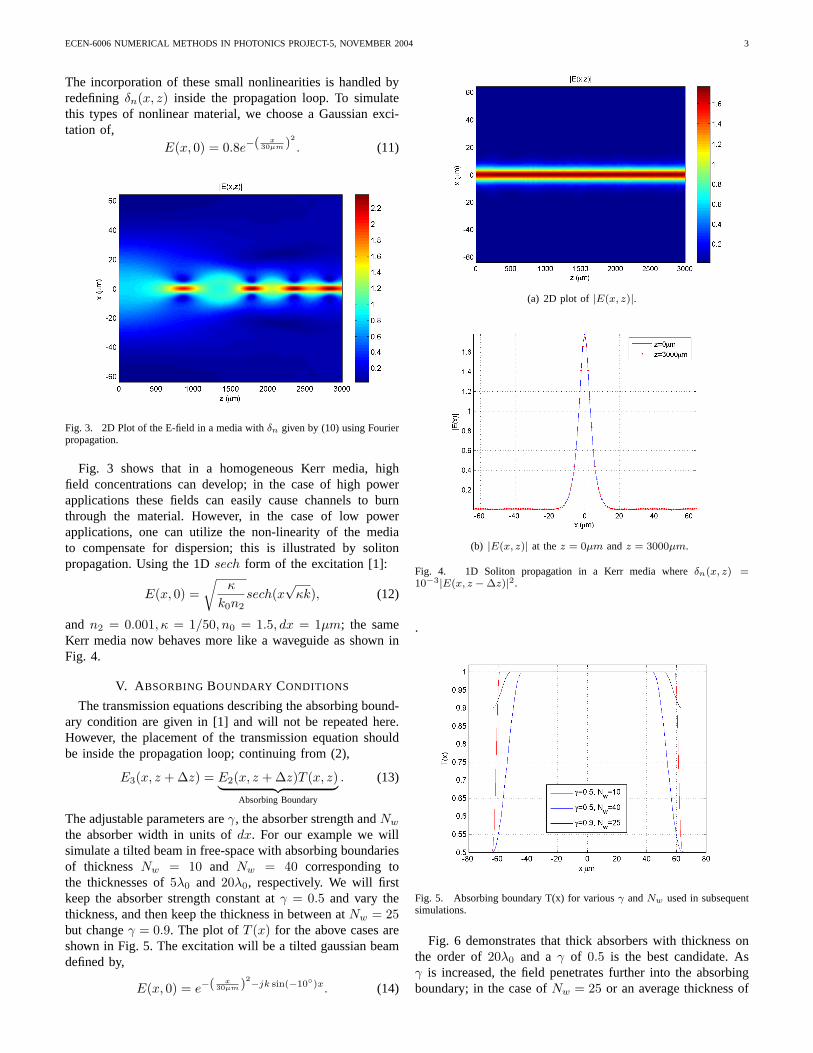
The incorporation of these small nonlinearities is handled byredefiningδn(x, z) inside the propagation loop. To simulatethis types of nonlinear material, we choose a Gaussian exci-tation of,

E(x, 0) = 0.8e−( x30µm )2

. (11)

Fig. 3. 2D Plot of the E-field in a media withδn given by (10) using Fourierpropagation.

Fig. 3 shows that in a homogeneous Kerr media, highfield concentrations can develop; in the case of high powerapplications these fields can easily cause channels to burnthrough the material. However, in the case of low powerapplications, one can utilize the non-linearity of the mediato compensate for dispersion; this is illustrated by solitonpropagation. Using the 1Dsech form of the excitation [1]:

E(x, 0) =√

κ

k0n2sech(x

√κk), (12)

and n2 = 0.001, κ = 1/50, n0 = 1.5, dx = 1µm; the sameKerr media now behaves more like a waveguide as shown inFig. 4.

V. A BSORBINGBOUNDARY CONDITIONS

The transmission equations describing the absorbing bound-ary condition are given in [1] and will not be repeated here.However, the placement of the transmission equation shouldbe inside the propagation loop; continuing from (2),

E3(x, z + ∆z) = E2(x, z + ∆z)T (x, z)︸ ︷︷ ︸Absorbing Boundary

. (13)

The adjustable parameters areγ, the absorber strength andNw

the absorber width in units ofdx. For our example we willsimulate a tilted beam in free-space with absorbing boundariesof thicknessNw = 10 and Nw = 40 corresponding tothe thicknesses of5λ0 and 20λ0, respectively. We will firstkeep the absorber strength constant atγ = 0.5 and vary thethickness, and then keep the thickness in between atNw = 25but changeγ = 0.9. The plot ofT (x) for the above cases areshown in Fig. 5. The excitation will be a tilted gaussian beamdefined by,

E(x, 0) = e−( x30µm )2−jk sin(−10◦)x. (14)

(a) 2D plot of |E(x, z)|.

(b) |E(x, z)| at thez = 0µm andz = 3000µm.

Fig. 4. 1D Soliton propagation in a Kerr media whereδn(x, z) =10−3|E(x, z − ∆z)|2.

.

Fig. 5. Absorbing boundary T(x) for variousγ andNw used in subsequentsimulations.

Fig. 6 demonstrates that thick absorbers with thickness onthe order of20λ0 and aγ of 0.5 is the best candidate. Asγ is increased, the field penetrates further into the absorbingboundary; in the case ofNw = 25 or an average thickness of

ECEN-6006 NUMERICAL METHODS IN PHOTONICS PROJECT-5, NOVEMBER 2004 4

12.5λ0 shown in Fig. 6(c), this over reach produced a faintperiodic reproduction of the original tilted beam. Significantreflection occurs when the thickness of the absorber is lessthan 10λ0 thick as shown in Fig. 6(a). In general, reflectionis more sensitive to the thickness of the absorberNw than theabsorber strength parameterγ.

(a) 2D plot of |E(x, z)|, γ = 0.5, Nw = 10.

(b) 2D plot of |E(x, z)|, γ = 0.5, Nw = 40.

(c) 2D plot of |E(x, z)|, γ = 0.9, Nw = 25.

Fig. 6. Absorbing boundary parameters and their effects on|E(x, z)|, dx =0.5λ0, dz = 2λ0.

VI. V OLUME HOLOGRAPHY

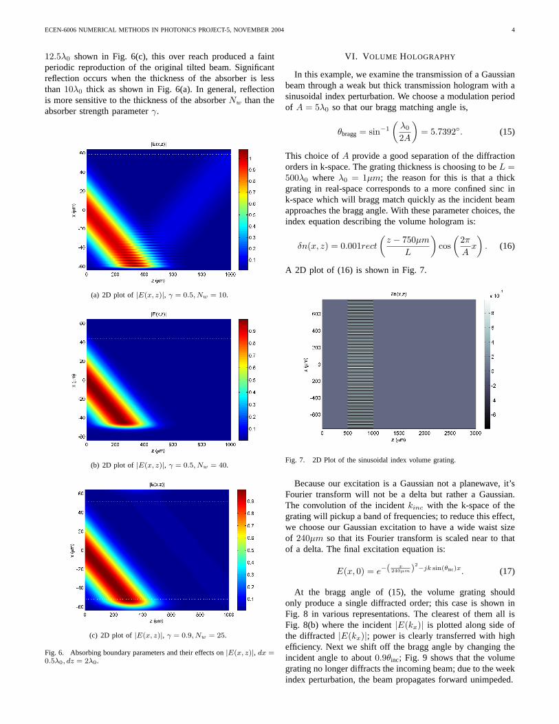
In this example, we examine the transmission of a Gaussianbeam through a weak but thick transmission hologram with asinusoidal index perturbation. We choose a modulation periodof A = 5λ0 so that our bragg matching angle is,

θbragg= sin−1

(λ0

2A

)= 5.7392◦. (15)

This choice ofA provide a good separation of the diffractionorders in k-space. The grating thickness is choosing to beL =500λ0 whereλ0 = 1µm; the reason for this is that a thickgrating in real-space corresponds to a more confined sinc ink-space which will bragg match quickly as the incident beamapproaches the bragg angle. With these parameter choices, theindex equation describing the volume hologram is:

δn(x, z) = 0.001rect

(z − 750µm

L

)cos

(2π

Ax

). (16)

A 2D plot of (16) is shown in Fig. 7.

Fig. 7. 2D Plot of the sinusoidal index volume grating.

Because our excitation is a Gaussian not a planewave, it’sFourier transform will not be a delta but rather a Gaussian.The convolution of the incidentkinc with the k-space of thegrating will pickup a band of frequencies; to reduce this effect,we choose our Gaussian excitation to have a wide waist sizeof 240µm so that its Fourier transform is scaled near to thatof a delta. The final excitation equation is:

E(x, 0) = e−( x240µm )2−jk sin(θinc)x. (17)

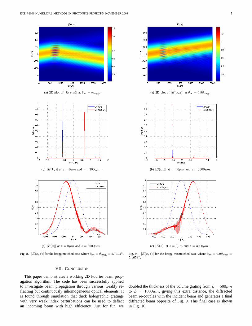
At the bragg angle of (15), the volume grating shouldonly produce a single diffracted order; this case is shown inFig. 8 in various representations. The clearest of them all isFig. 8(b) where the incident|E(kx)| is plotted along side ofthe diffracted|E(kx)|; power is clearly transferred with highefficiency. Next we shift off the bragg angle by changing theincident angle to about0.9θinc; Fig. 9 shows that the volumegrating no longer diffracts the incoming beam; due to the weekindex perturbation, the beam propagates forward unimpeded.

ECEN-6006 NUMERICAL METHODS IN PHOTONICS PROJECT-5, NOVEMBER 2004 5

(a) 2D plot of |E(x, z)| at θinc = θbragg.

(b) |E(kx)| at z = 0µm andz = 3000µm.

(c) |E(x)| at z = 0µm andz = 3000µm.

Fig. 8. |E(x, z)| for the bragg matched case whereθinc = θbragg = 5.7392◦.

VII. C ONCLUSION

This paper demonstrates a working 2D Fourier beam prop-agation algorithm. The code has been successfully appliedto investigate beam propagation through various weakly re-fracting but continuously inhomogeneous optical elements. Itis found through simulation that thick holographic gratingswith very weak index perturbations can be used to deflectan incoming beam with high efficiency. Just for fun, we

(a) 2D plot of |E(x, z)| at θinc = 0.9θbragg.

(b) |E(kx)| at z = 0µm andz = 3000µm.

(c) |E(x)| at z = 0µm andz = 3000µm.

Fig. 9. |E(x, z)| for the bragg mismatched case whereθinc = 0.9θbragg =5.1653◦.

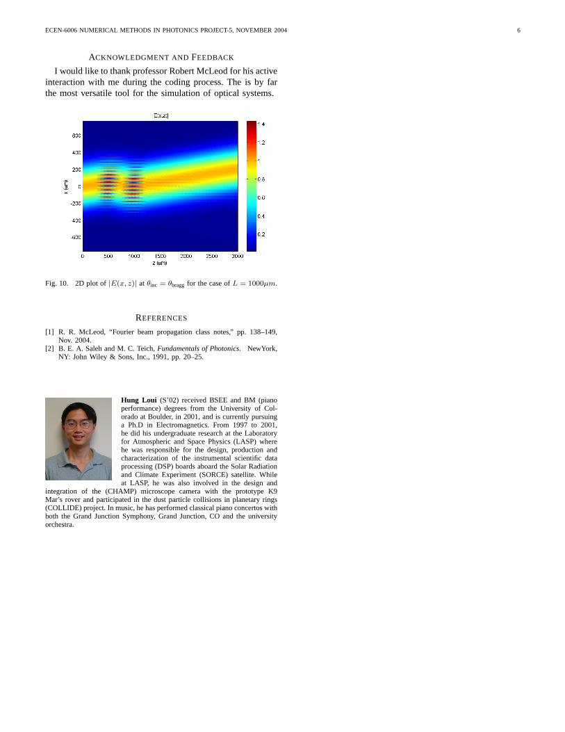
doubled the thickness of the volume grating fromL = 500µmto L = 1000µm, giving this extra distance, the diffractedbeam re-couples with the incident beam and generates a finaldiffracted beam opposite of Fig. 9. This final case is shownin Fig. 10.

ECEN-6006 NUMERICAL METHODS IN PHOTONICS PROJECT-5, NOVEMBER 2004 6

ACKNOWLEDGMENT AND FEEDBACK

I would like to thank professor Robert McLeod for his activeinteraction with me during the coding process. The is by farthe most versatile tool for the simulation of optical systems.

Fig. 10. 2D plot of|E(x, z)| at θinc = θbragg for the case ofL = 1000µm.

REFERENCES

[1] R. R. McLeod, “Fourier beam propagation class notes,” pp. 138–149,Nov. 2004.

[2] B. E. A. Saleh and M. C. Teich,Fundamentals of Photonics. NewYork,NY: John Wiley & Sons, Inc., 1991, pp. 20–25.

Hung Loui (S’02) received BSEE and BM (pianoperformance) degrees from the University of Col-orado at Boulder, in 2001, and is currently pursuinga Ph.D in Electromagnetics. From 1997 to 2001,he did his undergraduate research at the Laboratoryfor Atmospheric and Space Physics (LASP) wherehe was responsible for the design, production andcharacterization of the instrumental scientific dataprocessing (DSP) boards aboard the Solar Radiationand Climate Experiment (SORCE) satellite. Whileat LASP, he was also involved in the design and

integration of the (CHAMP) microscope camera with the prototype K9Mar’s rover and participated in the dust particle collisions in planetary rings(COLLIDE) project. In music, he has performed classical piano concertos withboth the Grand Junction Symphony, Grand Junction, CO and the universityorchestra.