Embed Size (px)
Citation preview

1/58
�
�
�
�
�
�
Math 45, Linear Algebra
Fourier Series
The Professor and The SaucemanCollege of the Redwoodse-mail: [email protected]

2/58
�
�
�
�
�
�
Objectives
• To show that the vector space containing all continuousfunctions is an innerproduct space.

3/58
�
�
�
�
�
�
Objectives
• To show that the vector space containing all continuousfunctions is an innerproduct space.
• Show that the set
{1, sin x, cos x, sin 2x, cos 2x, · · · , sin nx, cos nx, · · · }
are mutually orthogonal on the vector space C[0, 2π].

4/58
�
�
�
�
�
�
Objectives
• To show that the vector space containing all continuousfunctions is an innerproduct space.
• Show that the set
{1, sin x, cos x, sin 2x, cos 2x, · · · , sin nx, cos nx, · · · }
are mutually orthogonal on the vector space C[0, 2π].
• Create an orthonormal set by dividing each element by itsmagnitude.

5/58
�
�
�
�
�
�
Objectives
• To show that the vector space containing all continuousfunctions is an innerproduct space.
• Show that the set
{1, sin x, cos x, sin 2x, cos 2x, · · · , sin nx, cos nx, · · · }
are mutually orthogonal on the vector space C[0, 2π].
• Create an orthonormal set by dividing each element by itsmagnitude.
• To mathematically derive the Fourier Series as aprojection.

6/58
�
�
�
�
�
�
Objectives
• To show that the vector space containing all continuousfunctions is an innerproduct space.
• Show that the set
{1, sin x, cos x, sin 2x, cos 2x, · · · , sin nx, cos nx, · · · }
are mutually orthogonal on the vector space C[0, 2π].
• Create an orthonormal set by dividing each element by itsmagnitude.
• To mathematically derive the Fourier Series as aprojection.
• An Example: Project a function onto the space spannedby our orthonormal set.

7/58
�
�
�
�
�
�
The Vector Spaces
• A 3 dimensional vector lives in the vector space R3. Usually this is
what we deal with in linear algebra, that or R4, Rn, etc.
y
z
x
vR3
8/58
�
�
�
�
�
�
• All continuous functions also live in a vector space. On the interval
from a to b, that space is notated as C[a,b].
x
y
a bC [a, b]
f
g
• It would be easy to show that the ten properties of a vector space
are satisfied by this space.
• For any vectors f and g in C[a,b], the inner product is notated as
< f, g > and is defined to be∫ b
a f (x)g(x)dx.
9/58
�
�
�
�
�
�
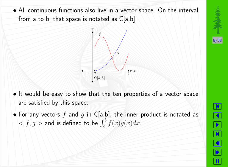
For C[a,b] to to be an inner product space, in addition to satisfying
the ten properties of a vector space, < f, g > must satisfy the following
conditions of inner products:
1. < f, f >≥ 0
2. < f, f > = 0 if and only if f = 0
3. < f, g > = < g, f >
4. < αf, g > = < f, αg >= α < f, g >
5. < f, g + h > = < f, g > + < f, h >
By using the definition of an inner product, < f, g > =∫ b
a f (x)g(x)dx,
each of these can be easily shown.
10/58
�
�
�
�
�
�
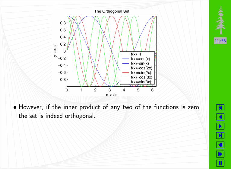
“Orthogonal is Good”
{1, cos x, sin x, cos 2x, sin 2x, cos 3x, sin 3x, · · · }
• For this set to be orthogonal in C[0,2π], every single term must be
orthogonal to every other one in that space.
• They certainly don’t look orthogonal, or at least not orthogonal as
we are used to.
11/58
�
�
�
�
�
�
0 1 2 3 4 5 6
−0.8
−0.6
−0.4
−0.2
0
0.2
0.4
0.6
0.8
x−axis
y−ax
is
The Orthogonal Set
f(x)=1 f(x)=cos(x) f(x)=sin(x) f(x)=cos(2x)f(x)=sin(2x)f(x)=cos(3x)f(x)=sin(3x)
• However, if the inner product of any two of the functions is zero,
the set is indeed orthogonal.
12/58
�
�
�
�
�
�
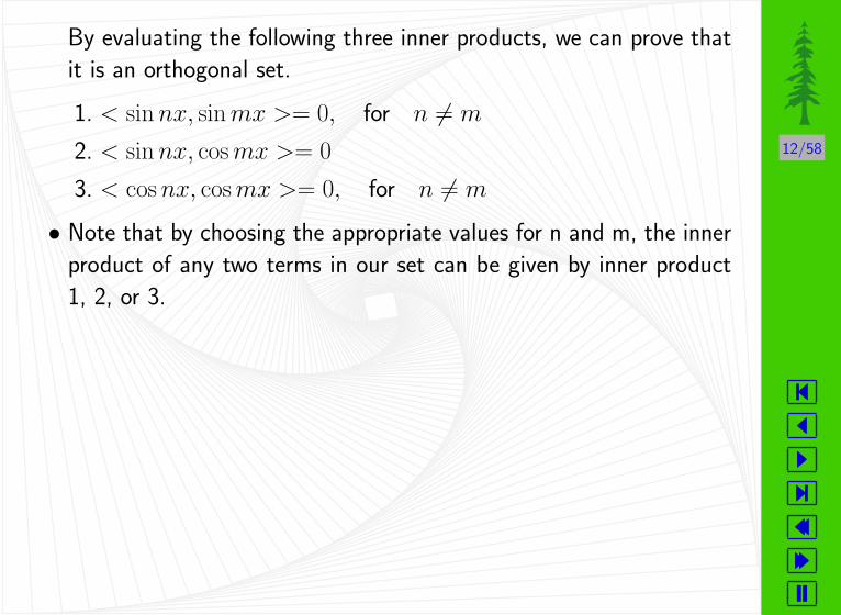
By evaluating the following three inner products, we can prove that
it is an orthogonal set.
1. < sin nx, sin mx >= 0, for n 6= m
2. < sin nx, cos mx >= 0
3. < cos nx, cos mx >= 0, for n 6= m
• Note that by choosing the appropriate values for n and m, the inner
product of any two terms in our set can be given by inner product
1, 2, or 3.
13/58
�
�
�
�
�
�
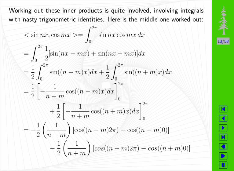
Working out these inner products is quite involved, involving integrals
with nasty trigonometric identities. Here is the middle one worked out:
< sin nx, cos mx >=
∫ 2π
0
sin nx cos mx dx
=
∫ 2π
0
1
2[sin(nx−mx) + sin(nx + mx)]dx
=1
2
∫ 2π
0
sin((n−m)x)dx +1
2
∫ 2π
0
sin((n + m)x)dx
=1
2
[− 1
n−mcos((n−m)x)dx
]2π
0
+1
2
[− 1
n + mcos((n + m)x)dx
]2π
0
= −1
2
(1
n−m
)[cos((n−m)2π) − cos((n−m)0)]
− 1
2
(1
n + m
)[cos((n + m)2π) − cos((n + m)0)]

14/58
�
�
�
�
�
�
< sin nx, cos mx > = −1
2
(1
n−m
)[1 − 1] − 1
2
(1
n + m
)[1 − 1]
= 0.
It turns out that no matter what the values of n and m, the inner product
is zero, so the vectors are orthogonal. The other two inner products are
evaluated similarly.

15/58
�
�
�
�
�
�
“Orthonormal is Better”

16/58
�
�
�
�
�
�
“Orthonormal is Better”
• To make the set orthonormal, calculate the magnitude of each vector
in the set, and then divide by it.

17/58
�
�
�
�
�
�
“Orthonormal is Better”
• To make the set orthonormal, calculate the magnitude of each vector
in the set, and then divide by it.
• First calculate the squared magnitude of each term by taking the
inner product of each vector with itself.

18/58
�
�
�
�
�
�
“Orthonormal is Better”
• To make the set orthonormal, calculate the magnitude of each vector
in the set, and then divide by it.
• First calculate the squared magnitude of each term by taking the
inner product of each vector with itself.
• The magnitudes squared of all sine vectors can be calculated in one
inner product,
‖ sin nx‖2 =< sin nx, sin nx >
=
∫ 2π
0
(sin nx)2dx
= π
19/58
�
�
�
�
�
�
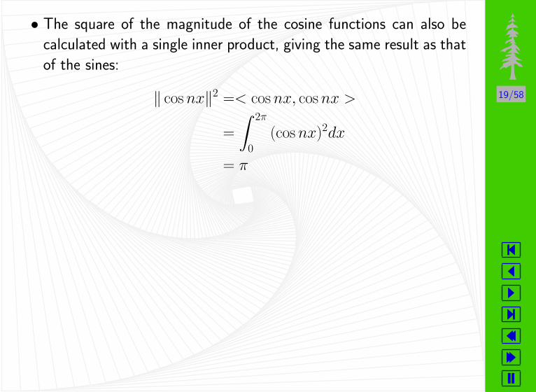
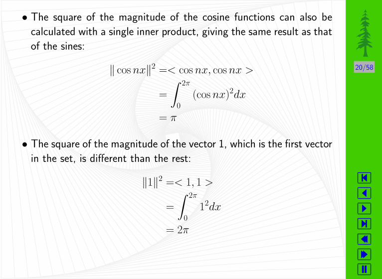
• The square of the magnitude of the cosine functions can also be
calculated with a single inner product, giving the same result as that
of the sines:
‖ cos nx‖2 =< cos nx, cos nx >
=
∫ 2π
0
(cos nx)2dx
= π
20/58
�
�
�
�
�
�
• The square of the magnitude of the cosine functions can also be
calculated with a single inner product, giving the same result as that
of the sines:
‖ cos nx‖2 =< cos nx, cos nx >
=
∫ 2π
0
(cos nx)2dx
= π
• The square of the magnitude of the vector 1, which is the first vector
in the set, is different than the rest:
‖1‖2 =< 1, 1 >
=
∫ 2π
0
12dx
= 2π
21/58
�
�
�
�
�
�
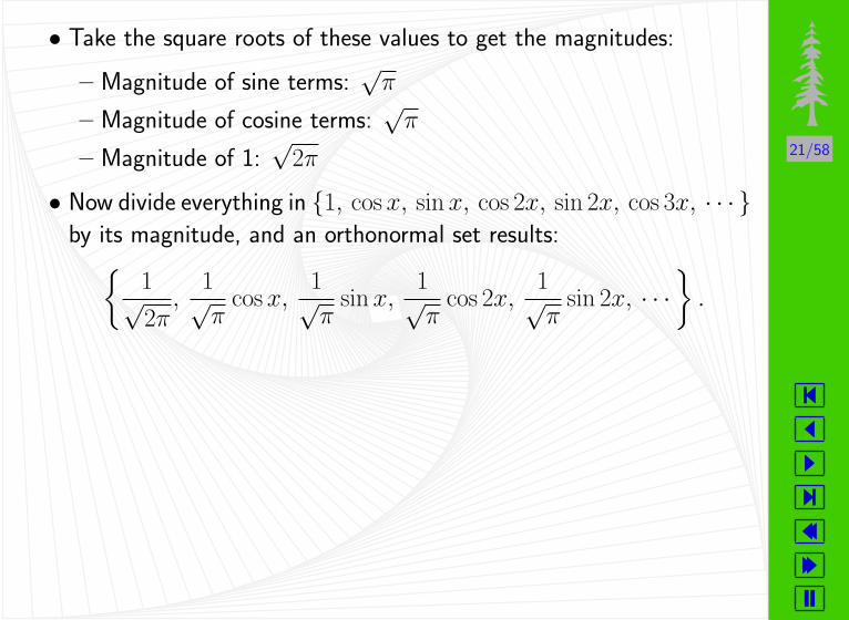
• Take the square roots of these values to get the magnitudes:
– Magnitude of sine terms:√
π
– Magnitude of cosine terms:√
π
– Magnitude of 1:√
2π
• Now divide everything in {1, cos x, sin x, cos 2x, sin 2x, cos 3x, · · · }by its magnitude, and an orthonormal set results:{
1√2π
,1√π
cos x,1√π
sin x,1√π
cos 2x,1√π
sin 2x, · · ·}
.
22/58
�
�
�
�
�
�
Projecting a Function Onto the SpaceSpanned by the Orthonormal set
• When a vector lives outside a vector space, what vector within the
space is closest to the outside vector? The answer to this is the
projection of that vector onto the space.
• Using the vectors from our orthonormal set as the basis, we can form
a space to project other functions onto.

23/58
�
�
�
�
�
�
• This is a little abstract, so first consider what it would mean to
project a 3 dimensional vector onto a space.
b
p
• The projection of a function onto a space spanned by functions is
the same idea, but graphically, it’s quite different. First we’ll show
mathematically how to do it, then we’ll give a graphical example.
24/58
�
�
�
�
�
�
The Math
First form a matrix Q with orthonormal columns. Using the idea of
least squares approximation, we will find that the projection of b onto
the space spanned by Q gives the vector in the space closest to b. The
formula for the projection onto the column space of Q is
p = Q(QTQ)−1QTb.
Since Q is an orthogonal matrix, (QTQ) = I . Thus,
p = QI−1QTb
= QQTb.
Continuing with our projection.

25/58
�
�
�
�
�
�
p =[q1 q2 q3 · · · qn
]qT
1
qT2
qT3...
qTn
b.

26/58
�
�
�
�
�
�
p =[q1 q2 q3 · · · q2n
]qT
1
qT2
qT3...
qTn
b.
= (q1qT1 + q2q
T2 + q3q
T3 + · · · + qnq
Tn )b

27/58
�
�
�
�
�
�
p =[q1 q2 q3 · · · qn
]qT
1
qT2
qT3...
qTn
b.
= (q1qT1 + q2q
T2 + q3q
T3 + · · · + qnq
Tn )b
= q1qT1 b + qnq
Tnb + q3q
T3 b + · · · + qnq
Tnb

28/58
�
�
�
�
�
�
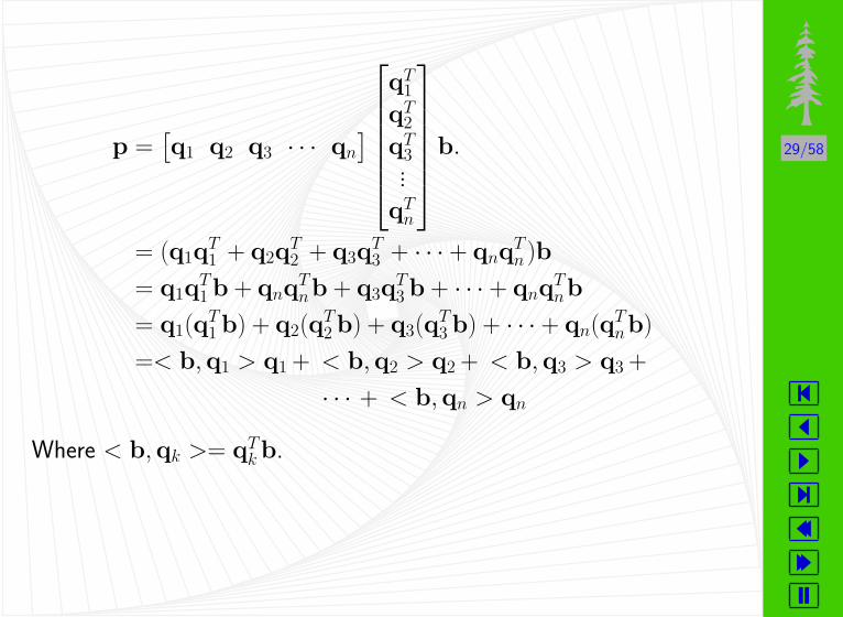
p =[q1 q2 q3 · · · qn
]qT
1
qT2
qT3...
qTn
b.
= (q1qT1 + q2q
T2 + q3q
T3 + · · · + qnq
Tn )b
= q1qT1 b + qnq
Tnb + q3q
T3 b + · · · + qnq
Tnb
= q1(qT1 b) + q2(q
T2 b) + q3(q
T3 b) + · · · + qn(qT
nb)
29/58
�
�
�
�
�
�
p =[q1 q2 q3 · · · qn
]qT
1
qT2
qT3...
qTn
b.
= (q1qT1 + q2q
T2 + q3q
T3 + · · · + qnq
Tn )b
= q1qT1 b + qnq
Tnb + q3q
T3 b + · · · + qnq
Tnb
= q1(qT1 b) + q2(q
T2 b) + q3(q
T3 b) + · · · + qn(qT
nb)
=< b,q1 > q1 + < b,q2 > q2 + < b,q3 > q3 +
· · · + < b,qn > qn
Where < b,qk >= qTk b.

30/58
�
�
�
�
�
�
Similarly, because V = C[0, 2π] is an innerproduct space, the projec-
tion of f onto the space spanned by our orthonormal set is
p =< f,1√2π
>1√2π
+ < f,1√π
cos x >1√π
cos x+ < f,1√π
sin x >1√π
sin x
+ · · ·
+ < f,1√π
cos nx >1√π
cos nx+ < f,1√π
sin nx >1√π
sin nx.

31/58
�
�
�
�
�
�
Similarly, because V = C[0, 2π] is an innerproduct space, the projec-
tion of f onto the space spanned by our orthonormal set is
p =< f,1√2π
>1√2π
+ < f,1√π
cos x >1√π
cos x+ < f,1√π
sin x >1√π
sin x
+ · · ·
+ < f,1√π
cos nx >1√π
cos nx+ < f,1√π
sin nx >1√π
sin nx.
Since all of the inner products produce constants, we label each
innerproduct with an ak and a bk.
p = a0 + a1 cos x + b1 sin x + · · · + an cos nx + bn sin nx

32/58
�
�
�
�
�
�
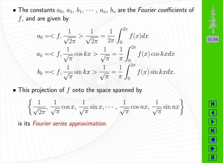
• The constants a0, a1, b1, · · · , an, bn are the Fourier coefficients of
f , and are given by
a0 =< f,1√2π
>1√2π
=1
2π
∫ 2π
0
f (x)dx
ak =< f,1√π
cos kx >1√π
=1
π
∫ 2π
0
f (x) cos kxdx
bk =< f,1√π
sin kx >1√π
=1
π
∫ 2π
0
f (x) sin kxdx.
33/58
�
�
�
�
�
�
• The constants a0, a1, b1, · · · , an, bn are the Fourier coefficients of
f , and are given by
a0 =< f,1√2π
>1√2π
=1
2π
∫ 2π
0
f (x)dx
ak =< f,1√π
cos kx >1√π
=1
π
∫ 2π
0
f (x) cos kxdx
bk =< f,1√π
sin kx >1√π
=1
π
∫ 2π
0
f (x) sin kxdx.
• This projection of f onto the space spanned by{1√2π
,1√π
cos x,1√π
sin x, · · · ,1√π
cos nx,1√π
sin nx
}is its Fourier series approximation.
34/58
�
�
�
�
�
�
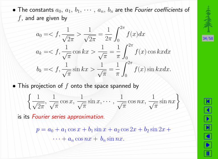
• The constants a0, a1, b1, · · · , an, bn are the Fourier coefficients of
f , and are given by
a0 =< f,1√2π
>1√2π
=1
2π
∫ 2π
0
f (x)dx
ak =< f,1√π
cos kx >1√π
=1
π
∫ 2π
0
f (x) cos kxdx
bk =< f,1√π
sin kx >1√π
=1
π
∫ 2π
0
f (x) sin kxdx.
• This projection of f onto the space spanned by{1√2π
,1√π
cos x,1√π
sin x, · · · ,1√π
cos nx,1√π
sin nx
}is its Fourier series approximation.
p = a0 + a1 cos x + b1 sin x + a2 cos 2x + b2 sin 2x +
· · · + an cos nx + bn sin nx.
35/58
�
�
�
�
�
�
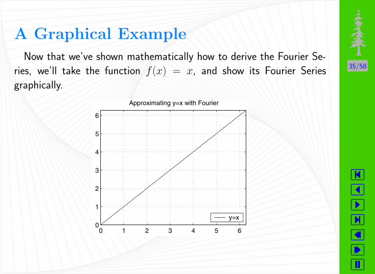
A Graphical Example
Now that we’ve shown mathematically how to derive the Fourier Se-
ries, we’ll take the function f (x) = x, and show its Fourier Series
graphically.
0 1 2 3 4 5 60
1
2
3
4
5
6
Approximating y=x with Fourier
y=x
36/58
�
�
�
�
�
�
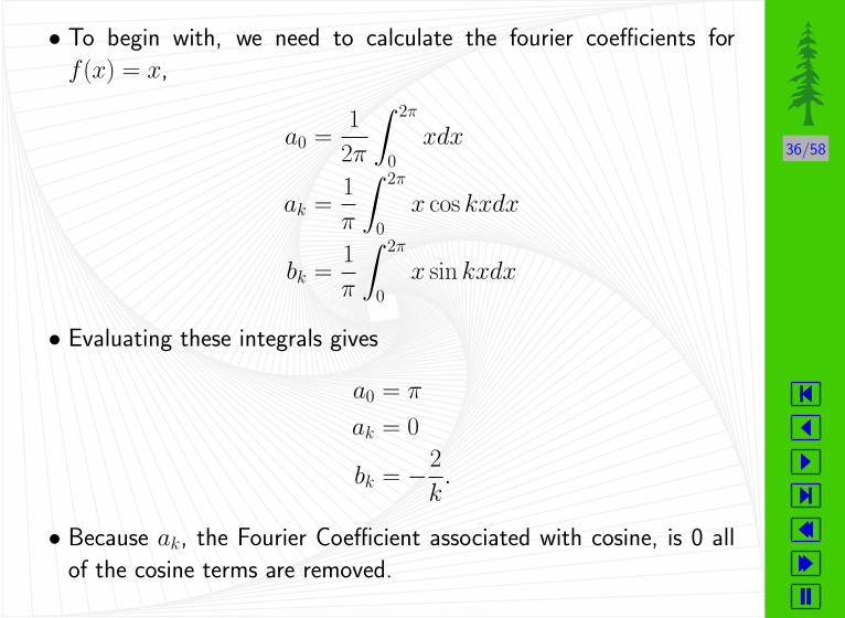
• To begin with, we need to calculate the fourier coefficients for
f (x) = x,
a0 =1
2π
∫ 2π
0
xdx
ak =1
π
∫ 2π
0
x cos kxdx
bk =1
π
∫ 2π
0
x sin kxdx
• Evaluating these integrals gives
a0 = π
ak = 0
bk = −2
k.
• Because ak, the Fourier Coefficient associated with cosine, is 0 all
of the cosine terms are removed.

37/58
�
�
�
�
�
�
• Then the projection of f (x) = x onto the space spanned by our
complete set becomes
p = π − 2 sin x− sin 2x− 2
3sin 3x− 1
2sin 4x− 2
5sin 5x− · · ·
• If we only use the first four vectors in our set as the basis for the
space we project onto,
B =
{1√2π
,1√π
cos x,1√π
sin x,1√π
cos 2x
},
we get the Fourier series with four terms, up through n = 3,
p = π − 2 sin x− sin 2x− 2
3sin 3x.

38/58
�
�
�
�
�
�
0 1 2 3 4 5 60
1
2
3
4
5
6
x−axis
y−ax
is
Approximating y=x with Fourier
y=x Fourier Approximation with n=3
• Note that we are only dealing with the vector space C[0, 2π].
Outside of that space has nothing to do with the projection.

39/58
�
�
�
�
�
�
• Now if we use the first 8 terms, up through n = 7, we get a function
that looks even more like f .
0 1 2 3 4 5 60
1
2
3
4
5
6
x−axis
y−ax
is
Approximating y=x with Fourier
y=x Fourier Approximation with n=7

40/58
�
�
�
�
�
�
• If the space we project onto has all the terms up through n = 50 as
the basis, the projection looks almost identical to f .
0 1 2 3 4 5 6
0
1
2
3
4
5
6
x−axis
y−ax
is
Approximating y=x with Fourier
y=x Fourier Approximation with n=50

41/58
�
�
�
�
�
�
• As clearly seen from the graphs, the more terms we use for basis for
the space we project onto, the more the similarity between f and its
projection. In other words, the more terms we include in the fourier
approximation, the better the approximation becomes.

42/58
�
�
�
�
�
�
Applications of the Fourier Series
• There are a wide range of application of Fourier Analysis within pure
mathematics. Such subjects are:
– Finding the sum of a series
– Isoperimetric problems
– Differential Equations
– Statistics
– The prime number theorem

43/58
�
�
�
�
�
�
• There are also applications within the field of physics. Some exam-
ples are:
– Quantum theory
– Lasers
– Electron Scattering
– Diffraction
– Telescopes
– Impedance

44/58
�
�
�
�
�
�
• Some applications in Chemistry include:
– Mass spectrometry
– NMR spectroscopy
– Infra-red spectroscopy
– Visible light spectroscopy
– Crystallography

45/58
�
�
�
�
�
�
• There even application in the life sciences. Some of which are:
– Vision
– Hearing
– Speech Analysis
– Morphogenesis
– Medical

46/58
�
�
�
�
�
�
• The applications of Fourier Analysis extends to many areas of the
sciences. Some miscellaneous applications are:
– Water Waves
– Turbulence in fluids
– Meteorology
– Glacier beds and “roughness”
– Seismology
– Vibration analysis
– Economics
• The list goes on and on.

47/58
�
�
�
�
�
�
Conclusion
• The vector space containing all continuous functions is an
innerproduct space.
48/58
�
�
�
�
�
�
Conclusion
• The vector space containing all continuous functions is an
innerproduct space.
• The set
{1, sin x, cos x, sin 2x, cos 2x, · · · , sin nx, cos nx, · · · }
are mutually orthogonal on the vector space C[0, 2π].

49/58
�
�
�
�
�
�
Conclusion
• The vector space containing all continuous functions is an
innerproduct space.
• The set
{1, sin x, cos x, sin 2x, cos 2x, · · · , sin nx, cos nx, · · · }
are mutually orthogonal on the vector space C[0, 2π].
• An orthonormal set is created by dividing each element by its
magnitude.
50/58
�
�
�
�
�
�
Conclusion
• The vector space containing all continuous functions is an
innerproduct space.
• The set
{1, sin x, cos x, sin 2x, cos 2x, · · · , sin nx, cos nx, · · · }
are mutually orthogonal on the vector space C[0, 2π].
• An orthonormal set is created by dividing each element by its
magnitude.
• The mathematical derivation of the Fourier Series is a projection.
51/58
�
�
�
�
�
�
Conclusion
• The vector space containing all continuous functions is an
innerproduct space.
• The set
{1, sin x, cos x, sin 2x, cos 2x, · · · , sin nx, cos nx, · · · }
are mutually orthogonal on the vector space C[0, 2π].
• An orthonormal set is created by dividing each element by its
magnitude.
• The mathematical derivation of the Fourier Series is a projection.
• The graphical example shows that an increased number of terms in
the projection decreases the error in the approximation.

52/58
�
�
�
�
�
�
References
[1] Strang, Gilbert. Introduction to Linear Algebra.
[2] Arnold, David. Fall 2001, Lectures and Insight by theMaster.
[3] Cartwright, Mark Fourier Methods for Mathematicians,Scientists and Engineers.