Embed Size (px)
Citation preview
Fourier Transform and its applicationsConvolutionCorrelation
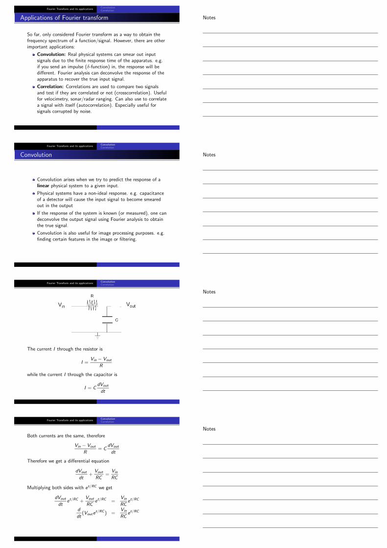
Applications of Fourier transform
So far, only considered Fourier transform as a way to obtain thefrequency spectrum of a function/signal. However, there are otherimportant applications:
Convolution: Real physical systems can smear out inputsignals due to the finite response time of the apparatus. e.g.if you send an impulse (δ-function) in, the response will bedifferent. Fourier analysis can deconvolve the response of theapparatus to recover the true input signal.
Correlation: Correlations are used to compare two signalsand test if they are correlated or not (crosscorrelation). Usefulfor velocimetry, sonar/radar ranging. Can also use to correlatea signal with itself (autocorrelation). Especially useful forsignals corrupted by noise.
Fourier Transform and its applicationsConvolutionCorrelation
Convolution
Convolution arises when we try to predict the response of alinear physical system to a given input.
Physical systems have a non-ideal response. e.g. capacitanceof a detector will cause the input signal to become smearedout in the output
If the response of the system is known (or measured), one candeconvolve the output signal using Fourier analysis to obtainthe true signal.
Convolution is also useful for image processing purposes. e.g.finding certain features in the image or filtering.
Fourier Transform and its applicationsConvolutionCorrelation
The current I through the resistor is
I =Vin − Vout
R
while the current I through the capacitor is
I = CdVout
dt
Fourier Transform and its applicationsConvolutionCorrelation
Both currents are the same, therefore
Vin − Vout
R= C
dVout
dt
Therefore we get a differential equation
dVout
dt+
Vout
RC=
Vin
RC
Multiplying both sides with et/RC we get
dVout
dtet/RC +
Vout
RCet/RC =
Vin
RCet/RC
d
dt(Voute
t/RC ) =Vin
RCet/RC
Notes
Notes
Notes
Notes
Fourier Transform and its applicationsConvolutionCorrelation
Integrating we obtain the analytic solution:
Vout(t) =e−t/RC
RC
[∫ t
−∞eτ/RCVin(τ)dτ + C1
](1)
=1
RC
∫ t
−∞e−(t−τ)/RCVin(τ)dτ (2)
where we put the constant of integration C1 = 0.
Now consider a δ-function input: Vin(t) = δ(t). Performing theintegration we get
Vout(t) =
{0, t < 0
1RC e
−t/RC , t = 0
Fourier Transform and its applicationsConvolutionCorrelation
Succession of δ pulses
Consider a train of δ function inputs. Since the system is linear,Vout is just the sum of the individual pulses. If they are closetogether they will overlap! The signal gets convolved with theexponential response.
Fourier Transform and its applicationsConvolutionCorrelation
As the pulse separation becomes smaller and smaller we pass tothe continuous case. We can write
Vin(t) =
∫ ∞−∞
Vin(τ)δ(t − τ)dτ
In our example, the response r(τ) to a δ pulse is just anexponential: r(τ) ∝ e−t/RC . The output can be written as
Vout(t) =
∫ ∞−∞
Vin(τ)r(t − τ)dτ (3)
= Vin ⊗ r (4)
which is the convolution of the input signal with the responsefunction of the system. (Compare with analytic solution eqn. (2)).
Fourier Transform and its applicationsConvolutionCorrelation
Convolution and Fourier transform
Convolution
p ⊗ q =1√2π
∫ ∞−∞
p(τ)q(t − τ)dτ (5)
What has this to do with Fourier transforms ? Let’s apply Fouriertransform to convolution:
F[p ⊗ q] =1√2π
∫ ∞−∞
[p ⊗ q]e−iωtdt
=1√2π
∫ ∞−∞
[1√2π
∫ ∞−∞
p(τ)q(t − τ)dτ
]e−iωtdt
=1√2π
∫ ∞−∞
p(τ)
[1√2π
∫ ∞−∞
q(t − τ)e−iωtdt
]dτ
Notes
Notes
Notes
Notes
Fourier Transform and its applicationsConvolutionCorrelation
Fourier convolution Theorem
Use shifting property of Fourier transform for the term in squarebrackets:
1√2π
∫ ∞−∞
q(t − τ)e−iωtdt = e−iωτQ(ω),
where Q(ω) = F[q]. Hence,
F[p ⊗ q] =1√2π
∫ ∞−∞
p(τ)e−iωτQ(ω)dτ
= P(ω)Q(ω)
Therefore,F[p ⊗ q] = F[p] · F[q] (6)
This is the Fourier convolution theorem: Convolution integralin the time domain is just a product in the frequency domain.
Fourier Transform and its applicationsConvolutionCorrelation
Fourier convolution Theorem
Typically, this is used to deconvolve a signal. If the system is linearand the response function r to a δ-pulse is known or measured wecan use the theorem to deconvolve the output signal Vout :
Vout = Vin ⊗ r
Therefore,F[Vout ] = F[Vin ⊗ r ] = F[Vin]F[r ]
And finally,
F[Vin] =F[Vout ]
F[r ]
or
Vin = F−1[F[Vout ]
F[r ]
]
Fourier Transform and its applicationsConvolutionCorrelation
Convolution - final remarks
Deconvolution only works for linear systems wheresuperposition holds.
Convolution is commutative: p ⊗ q = q ⊗ p
Many applications: “cleaning up” a smeared signal bydeconvolution; finding certain features in an image.
In real world applications, signal not only gets smeared out byresponse function, but also has noise on top of it. Can beaddressed using Wiener deconvolution (next week).
Fourier Transform and its applicationsConvolutionCorrelation
Correlation
Correlation provides a measure of similarity between two signals.Mathematically it is defined as
Correlation
p � q =1√2π
∫ ∞−∞
p∗(τ)q(t + τ)dτ (7)
Note the difference between correlation and convolution:
p ⊗ q =1√2π
∫ ∞−∞
p(τ)q(t − τ)dτ
Notes
Notes
Notes
Notes
Fourier Transform and its applicationsConvolutionCorrelation
The correlation is a function of the lag time t. A functioncorrelated with itself is called autocorrelation:
p � p =1√2π
∫ ∞−∞
p∗(τ)p(t + τ)dτ (8)
Unlike convolution, correlation is not commutative: p� q 6= q � p.
Fourier Transform and its applicationsConvolutionCorrelation
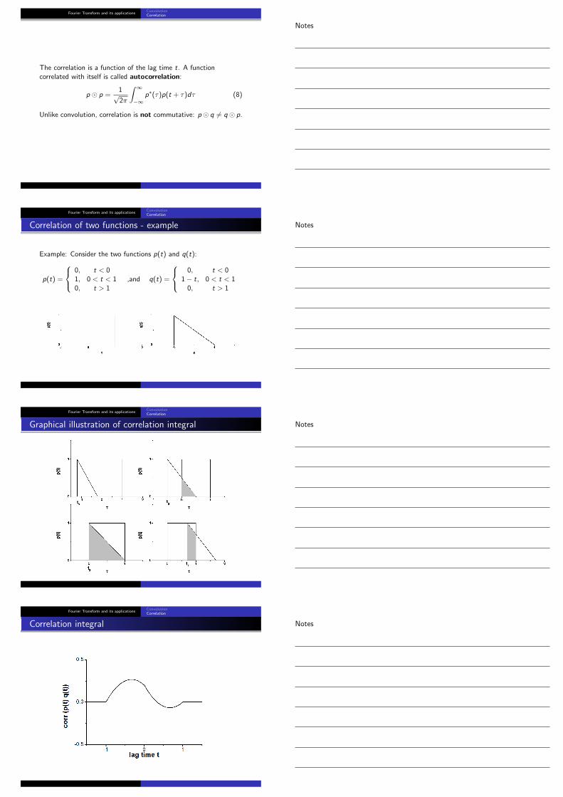
Correlation of two functions - example
Example: Consider the two functions p(t) and q(t):
p(t) =
0, t < 01, 0 < t < 10, t > 1
,and q(t) =
0, t < 0
1− t, 0 < t < 10, t > 1
Fourier Transform and its applicationsConvolutionCorrelation
Graphical illustration of correlation integral
Fourier Transform and its applicationsConvolutionCorrelation
Correlation integral
Notes
Notes
Notes
Notes
Fourier Transform and its applicationsConvolutionCorrelation
Average correlation function
If functions being correlated are not of finite duration and don’tvanish as t → ±∞, the correlation integral may not exist. In thiscase can define an average correlation function:
[p � q]avg = limT→∞
1
T
∫ T/2
−T/2p∗(τ)q(t + τ)dτ (9)
If functions p and q are periodic with period T0, set T = T0 inabove definition.
Fourier Transform and its applicationsConvolutionCorrelation
What does it mean if two functions are uncorrelated? Let’s write
p(t) = 〈p〉+ ∆p(t) , and q(t) = 〈q〉+ ∆q(t),
where we decomposed the functions into their mean and theirtime-dependent deviations from the mean ∆p(t). Also assumethat the functions are real.
[p � q]avg = limT→∞
1
T
∫ T/2
−T/2[〈p〉+ ∆p(τ)][〈q〉+ ∆q(t + τ)]dτ
= 〈p〉〈q〉+ 〈p〉 limT→∞
1
T
∫ T/2
−T/2∆q(t + τ)dτ
+〈q〉 limT→∞
1
T
∫ T/2
−T/2∆p(τ)dτ
+ limT→∞
1
T
∫ T/2
−T/2∆p(τ)∆q(t + τ)dτ
Fourier Transform and its applicationsConvolutionCorrelation
Uncorrelated functions
By definition,
limT→∞
1
T
∫ T/2
−T/2∆q(t + τ)dτ = lim
T→∞
1
T
∫ T/2
−T/2∆p(τ)dτ = 0,
since the deviations from the mean have to average to zero:
〈p〉 ≡ limT→∞
1
T
∫ T/2
−T/2p(τ)dτ = lim
T→∞
1
T
∫ T/2
−T/2[〈p〉+ ∆p(τ)]dτ
= 〈p〉+ limT→∞
1
T
∫ T/2
−T/2∆p(τ)dτ︸ ︷︷ ︸
=0
Fourier Transform and its applicationsConvolutionCorrelation
Uncorrelated functions
Since two terms are zero, the correlation function reduces to
[p � q]avg = 〈p〉〈q〉+ limT→∞
1
T
∫ T/2
−T/2∆p(τ)∆q(t + τ)dτ
If the variations in p are unrelated to the variations in q (e.g. ifone of them is noise), the integral on the right hand side will bezero and the functions are considered uncorrelated:
[p � q]avg = 〈p〉〈q〉
The correlation integral is constant and reduces to the product ofthe two mean values. In particular if the mean value of either p orq is zero, the correlation will be also zero. e.g. if one of them iswhite noise.
Notes
Notes
Notes
Notes
Fourier Transform and its applicationsConvolutionCorrelation
Example - Sonar/Radar ranging
By measuring the time delay between the transmission of a signaland the reception of its echo that bounces off an object, one caninfer the distance by knowing the speed of the wave.
Problem: Echo is weak, since intensity falls off as 1/r4. Moreover,echo corrupted by noise.
Solution: Rather than looking for the echo directly, cross-correlateecho with the original reference signal. Correlation will be large atthe lag time that corresponds to the travel time of the signal. Willshow that correlation works well even if signal/noise is low.
Fourier Transform and its applicationsConvolutionCorrelation
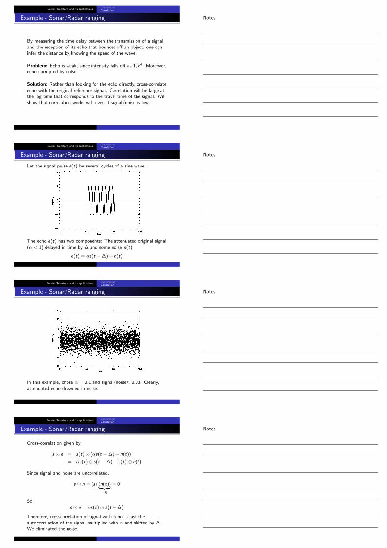
Example - Sonar/Radar ranging
Let the signal pulse s(t) be several cycles of a sine wave:
The echo e(t) has two components: The attenuated original signal(α < 1) delayed in time by ∆ and some noise n(t)
e(t) = αs(t −∆) + n(t)
Fourier Transform and its applicationsConvolutionCorrelation
Example - Sonar/Radar ranging
In this example, chose α = 0.1 and signal/noise≈ 0.03. Clearly,attenuated echo drowned in noise.
Fourier Transform and its applicationsConvolutionCorrelation
Example - Sonar/Radar ranging
Cross-correlation given by
s � e = s(t)� (αs(t −∆) + n(t))
= αs(t)� s(t −∆) + s(t)� n(t)
Since signal and noise are uncorrelated,
s � n = 〈s〉 〈n(t)〉︸ ︷︷ ︸=0
= 0
So,s � e = αs(t)� s(t −∆)
Therefore, crosscorrelation of signal with echo is just theautocorrelation of the signal multiplied with α and shifted by ∆.We eliminated the noise.
Notes
Notes
Notes
Notes
Fourier Transform and its applicationsConvolutionCorrelation
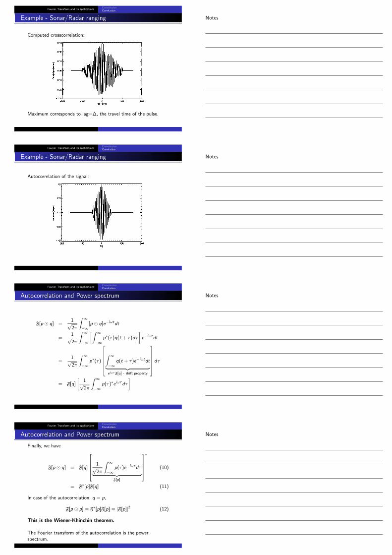
Example - Sonar/Radar ranging
Computed crosscorrelation:
Maximum corresponds to lag=∆, the travel time of the pulse.
Fourier Transform and its applicationsConvolutionCorrelation
Example - Sonar/Radar ranging
Autocorrelation of the signal:
Fourier Transform and its applicationsConvolutionCorrelation
Autocorrelation and Power spectrum
F[p � q] =1√2π
∫ ∞−∞
[p � q]e−iωtdt
=1√2π
∫ ∞−∞
[∫ ∞−∞
p∗(τ)q(t + τ)dτ
]e−iωtdt
=1√2π
∫ ∞−∞
p∗(τ)
∫ ∞−∞
q(t + τ)e−iωtdt︸ ︷︷ ︸e iωτF[q] - shift property
dτ
= F[q]
[1√2π
∫ ∞−∞
p(τ)∗e iωτdτ
]
Fourier Transform and its applicationsConvolutionCorrelation
Autocorrelation and Power spectrum
Finally, we have
F[p � q] = F[q]
1√2π
∫ ∞−∞
p(τ)e−iωτdτ︸ ︷︷ ︸F[p]
∗
(10)
= F∗[p]F[q] (11)
In case of the autocorrelation, q = p,
F[p � p] = F∗[p]F[p] = |F[p]|2 (12)
This is the Wiener-Khinchin theorem.
The Fourier transform of the autocorrelation is the powerspectrum.
Notes
Notes
Notes
Notes

Fourier Transform and its applicationsConvolutionCorrelation
Example
White noise is defined as
p � p = δ(t) (13)
Only non-zero correlation at lag t = 0. Use Wiener-Khinchin:
F[p � p] = F[δ(t)] =1√2π
Power spectrum is a constant. All frequencies occur equally. Thename “White noise” comes from white light, in which allfrequencies are present.
Fourier Transform and its applicationsConvolutionCorrelation
Summary
Both the convolution and correlation integral reduce to simpleproducts of the respective Fourier transform:
Convolution theorem:
F[p ⊗ q] = F[p] · F[q]
Wiener Khinchin theorem:
F[p � q] = F∗[p]F[q]
In higher dimensions it is computationally more efficient to performcorrelations and convolutions in Fourier space. This is due to theexistence of the Fast Fourier Transform (FFT) algorithm, which wediscuss next time.
Notes
Notes
Notes
Notes


![[PPT]Convolution, Fourier Series, and the Fourier …social.cs.uiuc.edu/.../lectures/Convolution_Fourier.ppt · Web viewConvolution, Fourier Series, and the Fourier Transform CS414](https://img.pdfslide.net/doc/110x75/5b911edf09d3f2b6628d8b14/pptconvolution-fourier-series-and-the-fourier-web-viewconvolution-fourier.jpg)