Embed Size (px)
Citation preview
Fourier Transform
in
Image Processing
CS6640, Fall 2012
Guest Lecture
Marcel Prastawa, SCI Utah

Preliminaries
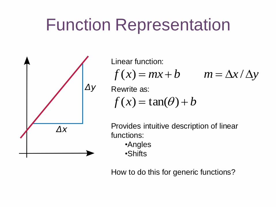
Function Representation
Linear function:
Rewrite as:
Provides intuitive description of linear
functions:
•Angles
•Shifts
How to do this for generic functions?
bmxxf )(
bxf )tan()(
yxm /
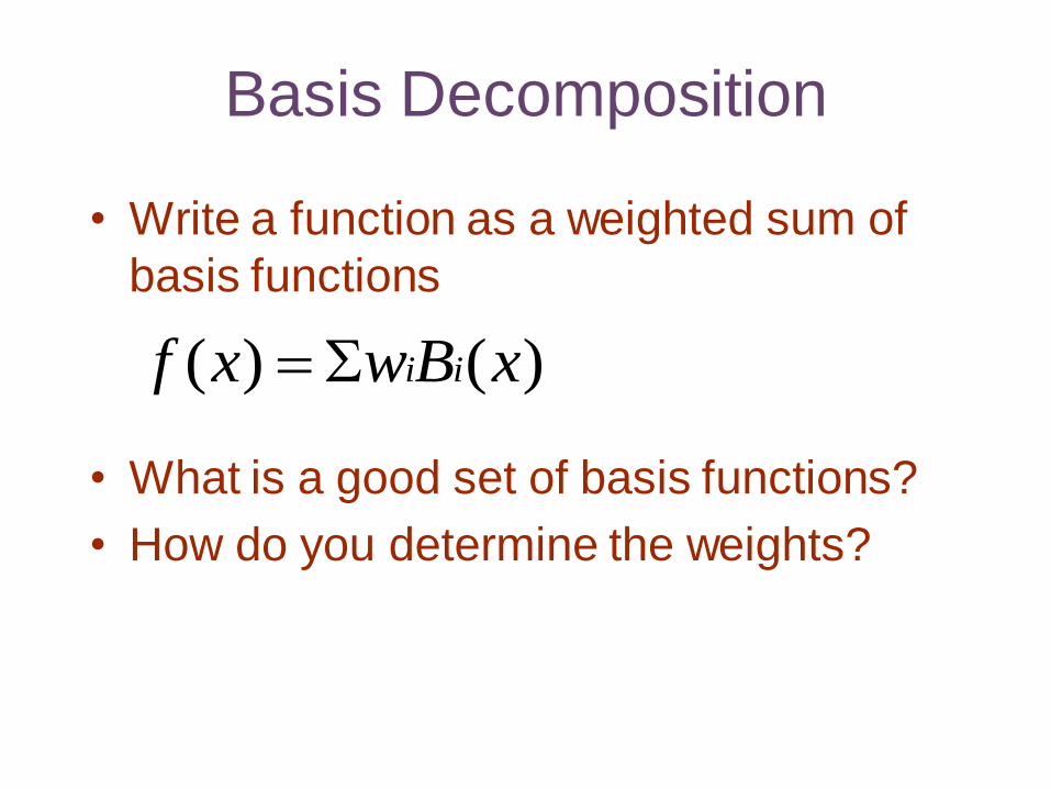
Basis Decomposition
• Write a function as a weighted sum of
basis functions
• What is a good set of basis functions?
• How do you determine the weights?
)()( xBwxf ii
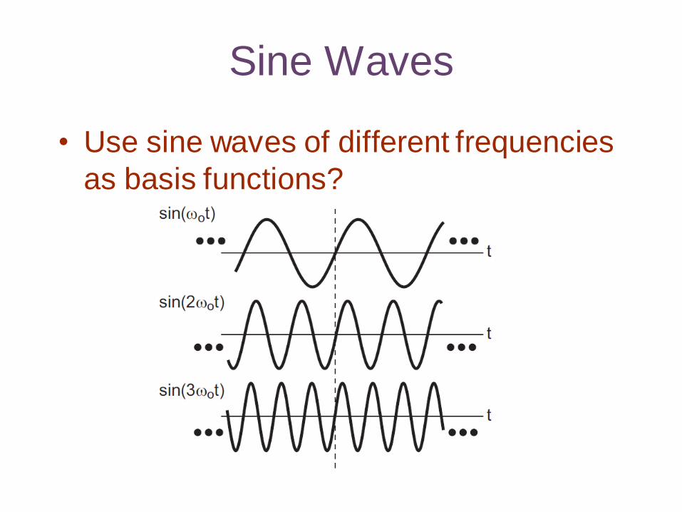
Sine Waves
• Use sine waves of different frequencies
as basis functions?
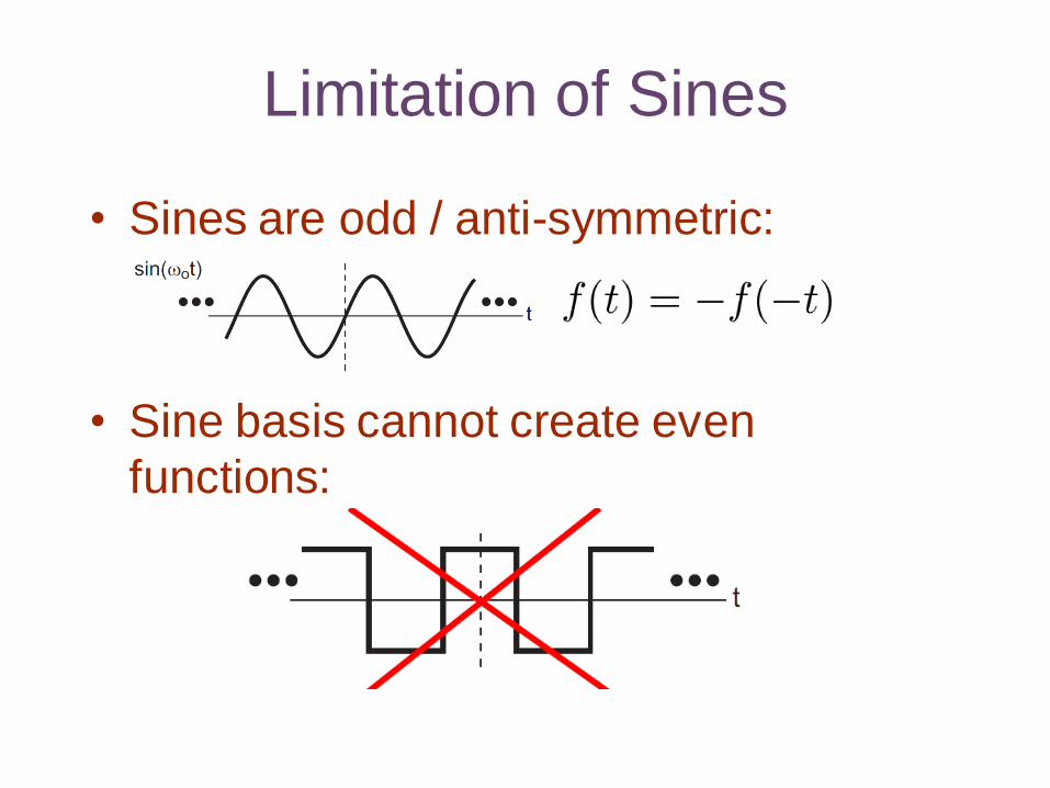
Limitation of Sines
• Sines are odd / anti-symmetric:
• Sine basis cannot create even
functions:
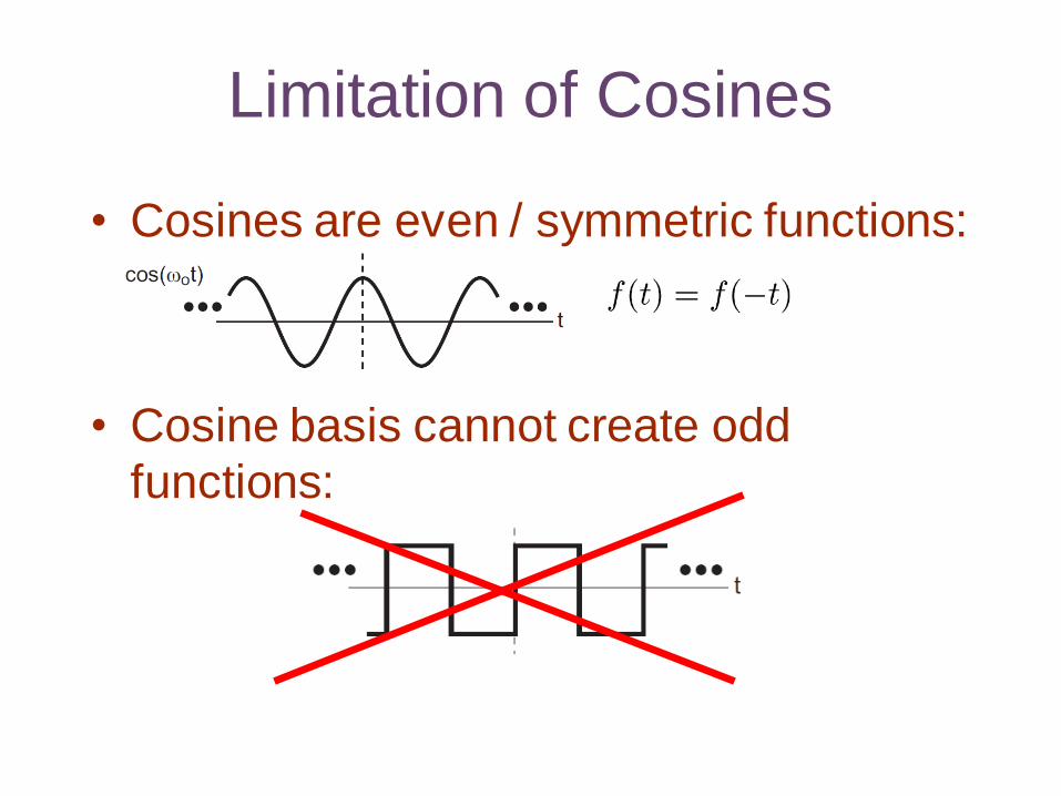
Limitation of Cosines
• Cosines are even / symmetric functions:
• Cosine basis cannot create odd
functions:
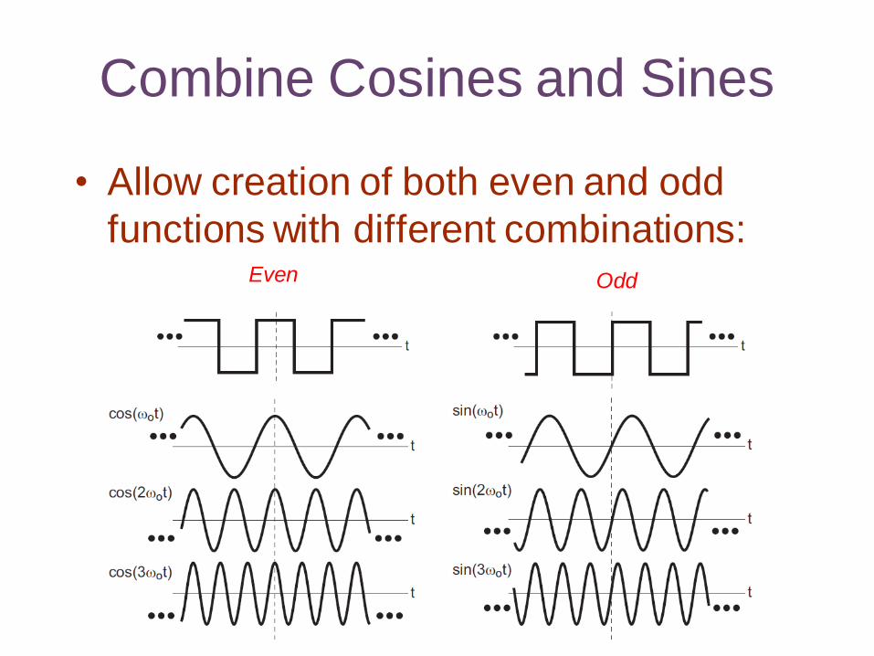
Combine Cosines and Sines
• Allow creation of both even and odd
functions with different combinations: Odd Even
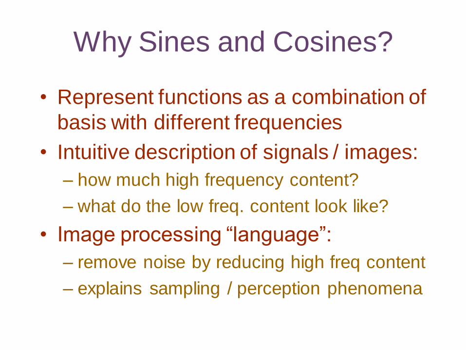
Why Sines and Cosines?
• Represent functions as a combination of
basis with different frequencies
• Intuitive description of signals / images:
– how much high frequency content?
– what do the low freq. content look like?
• Image processing “language”:
– remove noise by reducing high freq content
– explains sampling / perception phenomena
The Fourier Transform
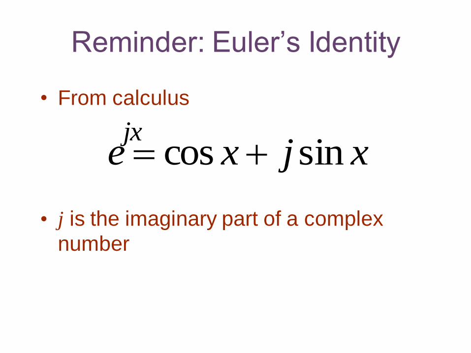
Reminder: Euler’s Identity
• From calculus
• j is the imaginary part of a complex
number
xjxe sincos jx
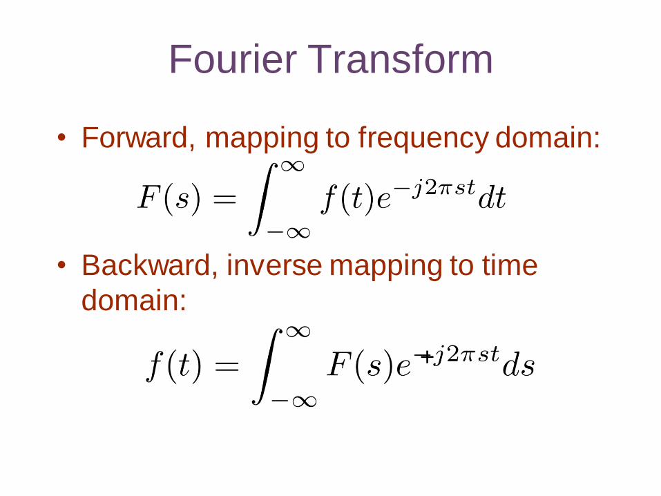
Fourier Transform
• Forward, mapping to frequency domain:
• Backward, inverse mapping to time
domain:
+
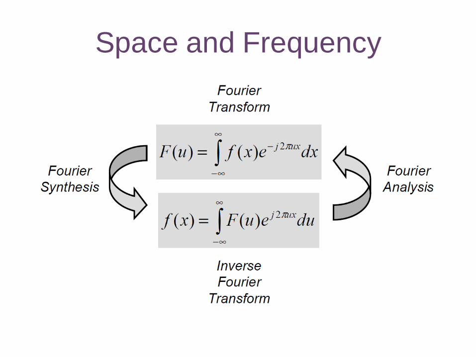
Space and Frequency
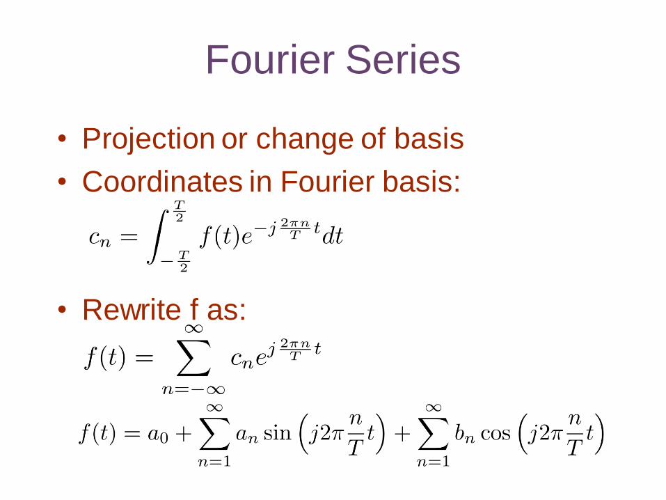
Fourier Series
• Projection or change of basis
• Coordinates in Fourier basis:
• Rewrite f as:
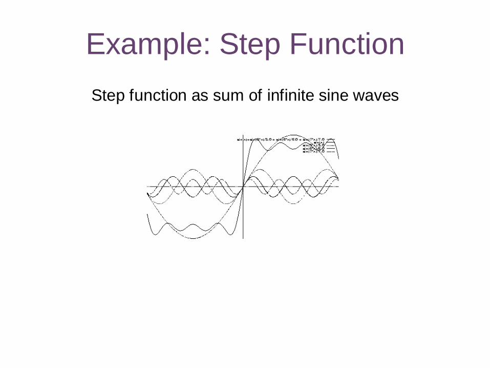
Example: Step Function
Step function as sum of infinite sine waves
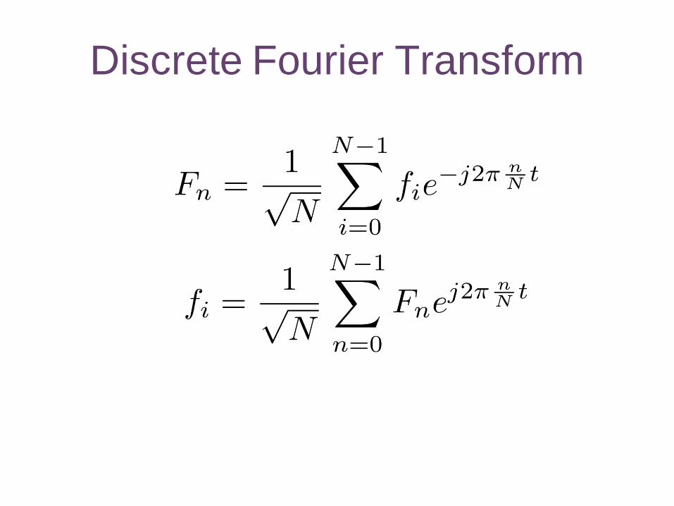
Discrete Fourier Transform
Fourier Basis
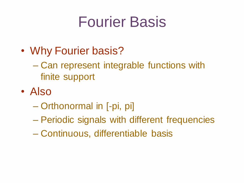
• Why Fourier basis?
– Can represent integrable functions with
finite support
• Also
– Orthonormal in [-pi, pi]
– Periodic signals with different frequencies
– Continuous, differentiable basis
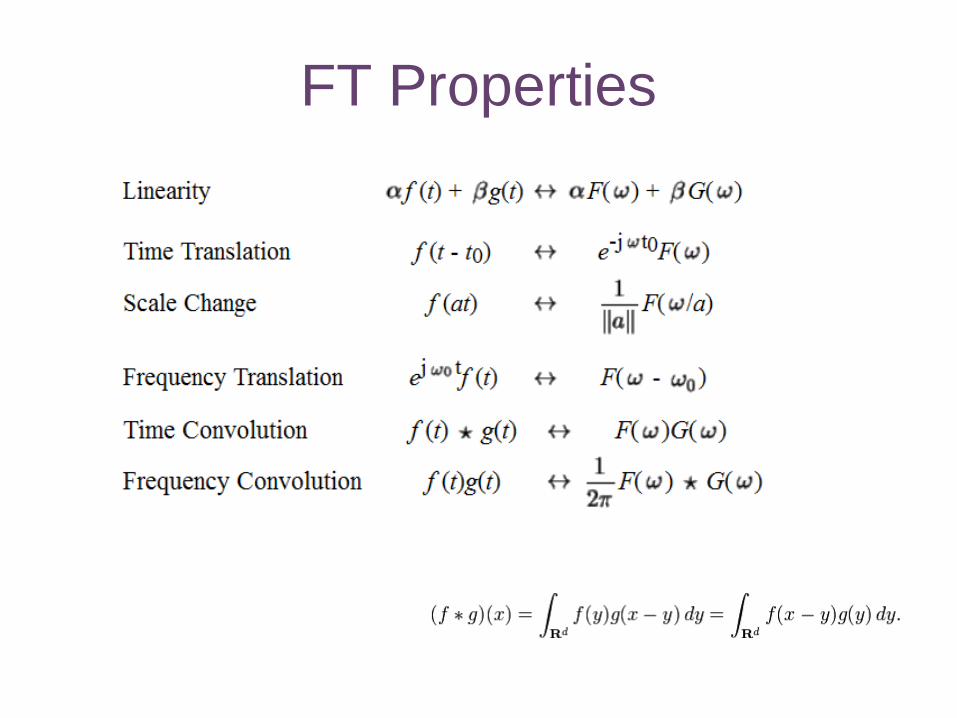
FT Properties
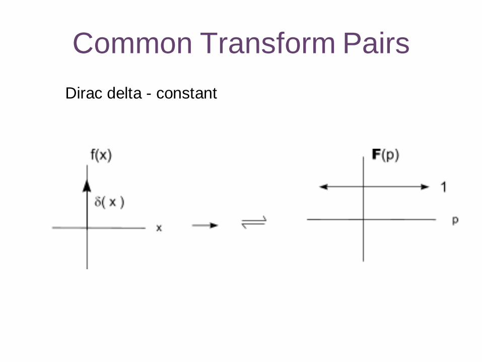
Common Transform Pairs
Dirac delta - constant
Common Transform Pairs
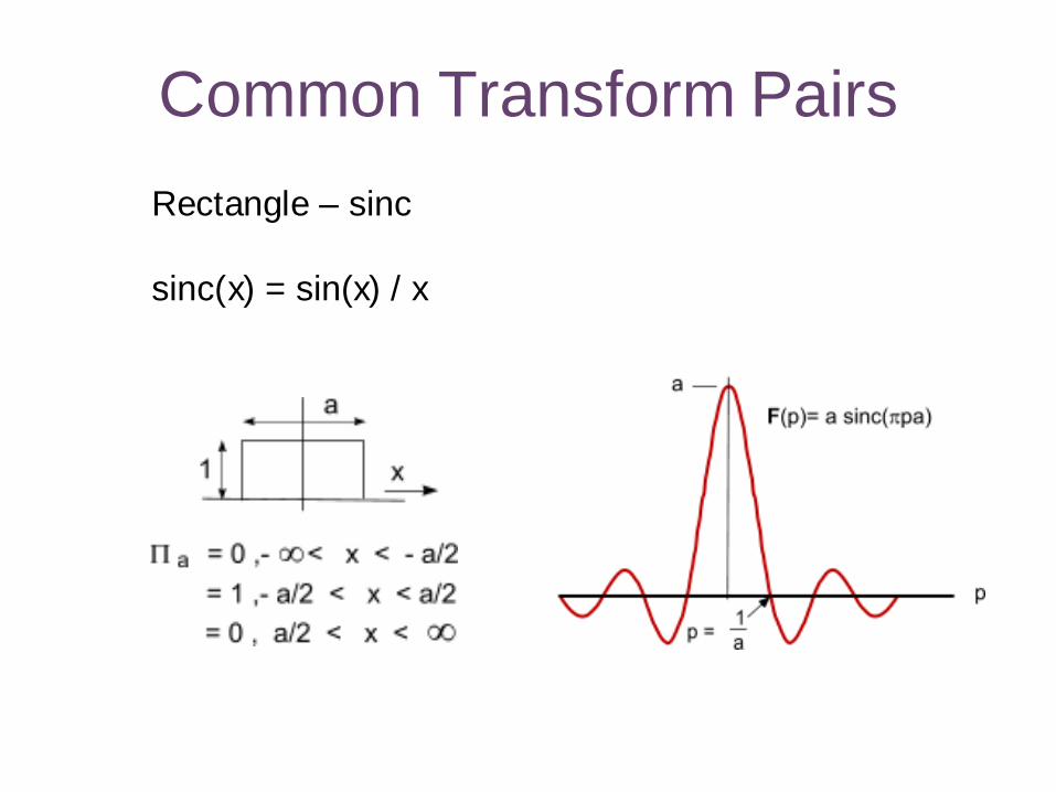
Rectangle – sinc
sinc(x) = sin(x) / x
Common Transform Pairs
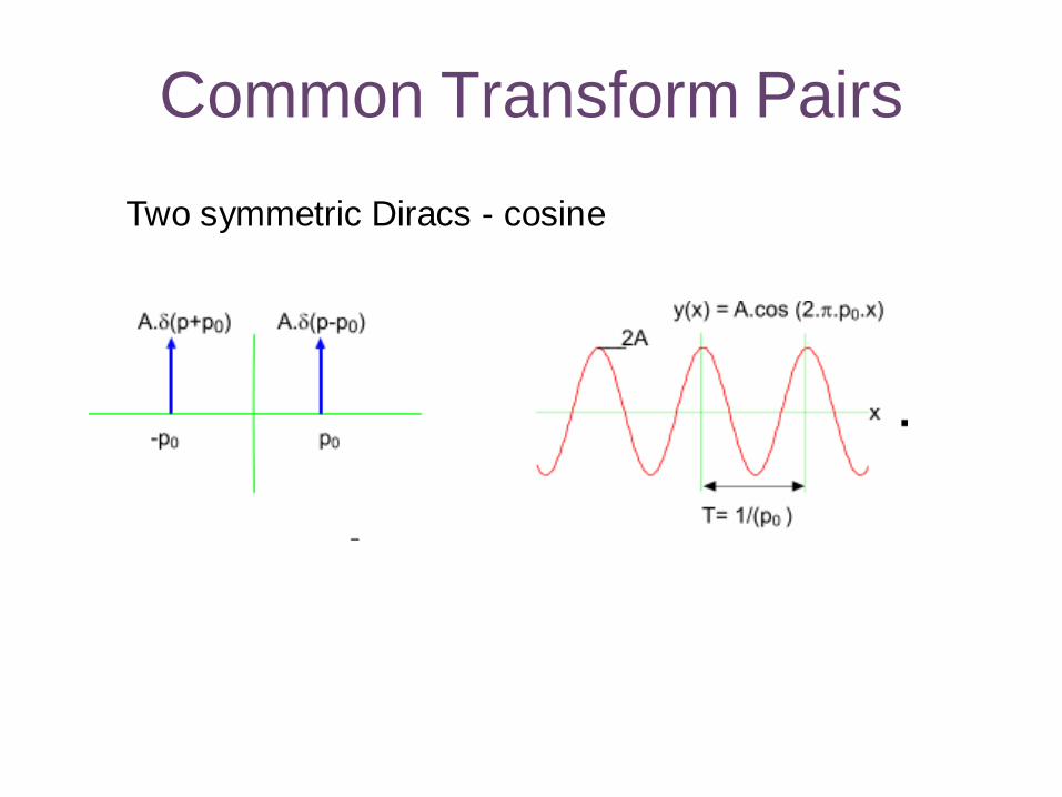
Two symmetric Diracs - cosine
Common Transform Pairs
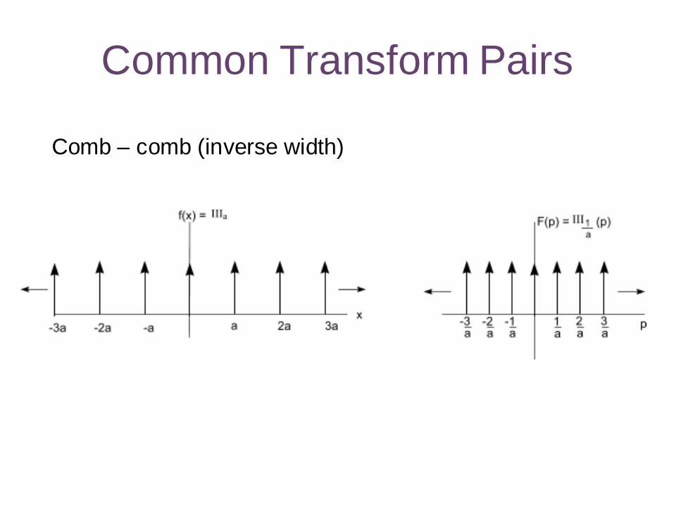
Comb – comb (inverse width)
Common Transform Pairs
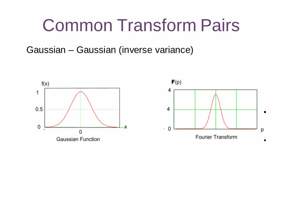
Gaussian – Gaussian (inverse variance)
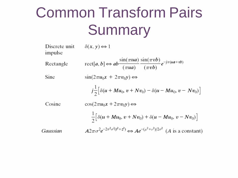
Common Transform Pairs
Summary
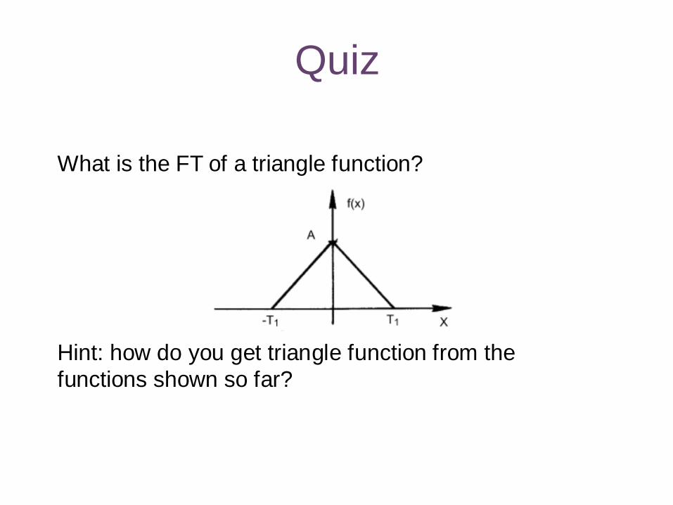
Quiz
What is the FT of a triangle function?
Hint: how do you get triangle function from the
functions shown so far?
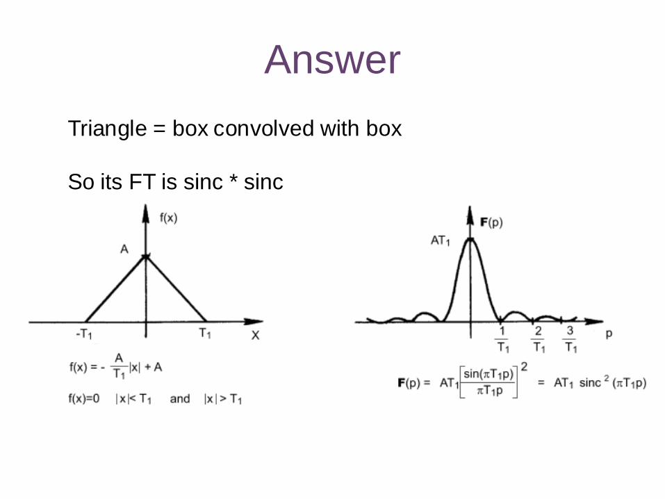
Answer
Triangle = box convolved with box
So its FT is sinc * sinc
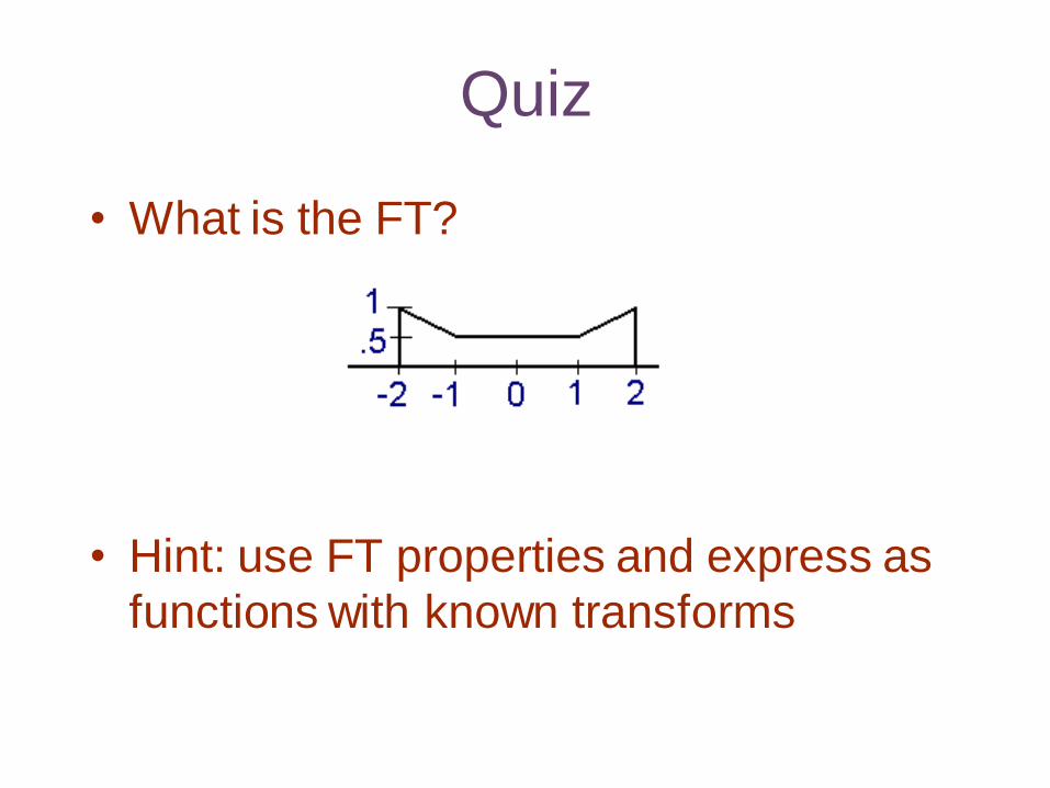
Quiz
• What is the FT?
• Hint: use FT properties and express as
functions with known transforms
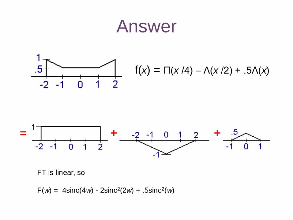
Answer
f(x) = Π(x /4) – Λ(x /2) + .5Λ(x)
FT is linear, so
F(w) = 4sinc(4w) - 2sinc2(2w) + .5sinc2(w)
Fourier Transform of Images
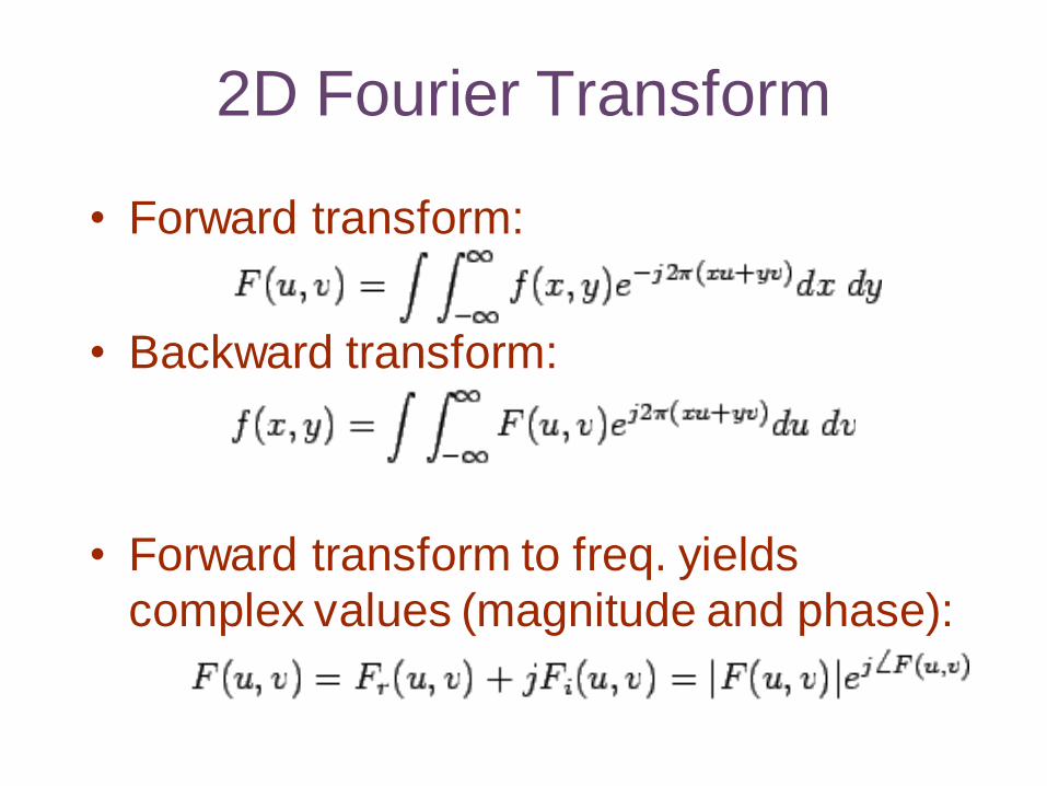
• Forward transform:
• Backward transform:
• Forward transform to freq. yields
complex values (magnitude and phase):
2D Fourier Transform
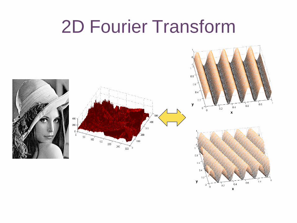
2D Fourier Transform
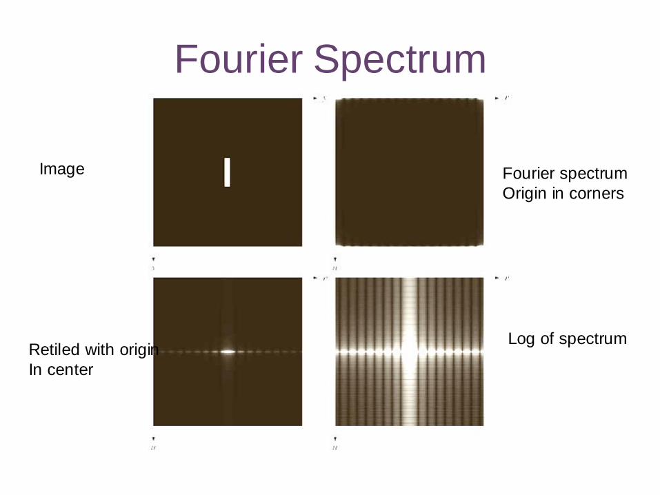
Fourier Spectrum
Fourier spectrum
Origin in corners
Retiled with origin
In center
Log of spectrum
Image
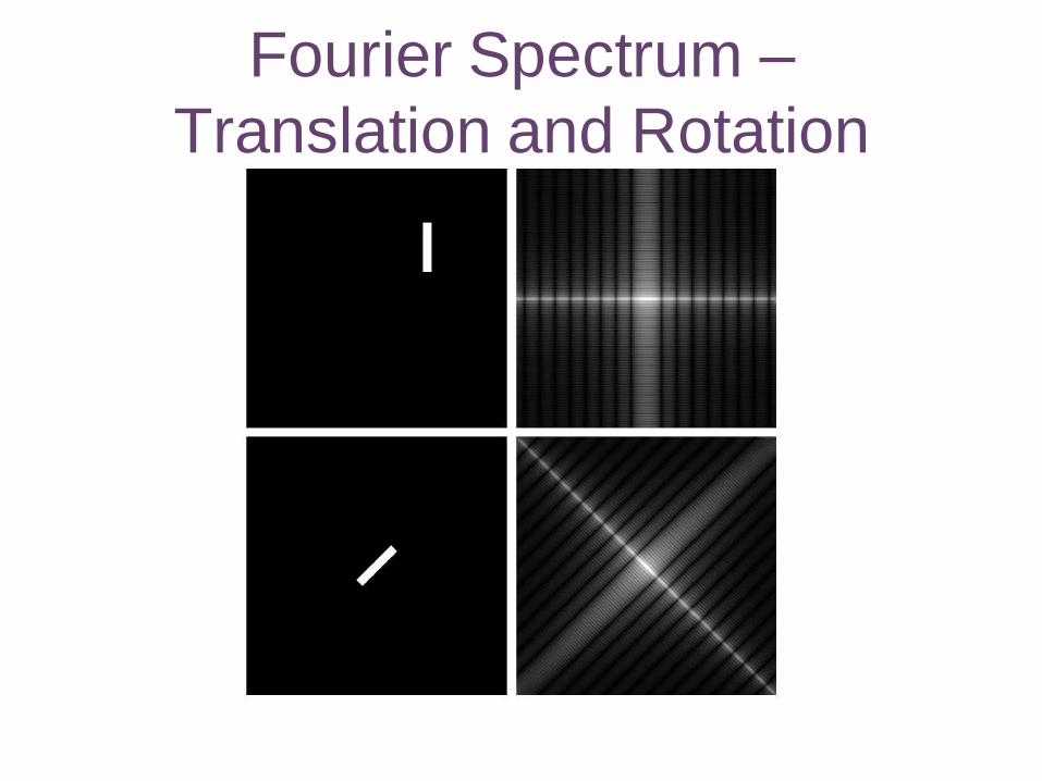
Fourier Spectrum –
Translation and Rotation
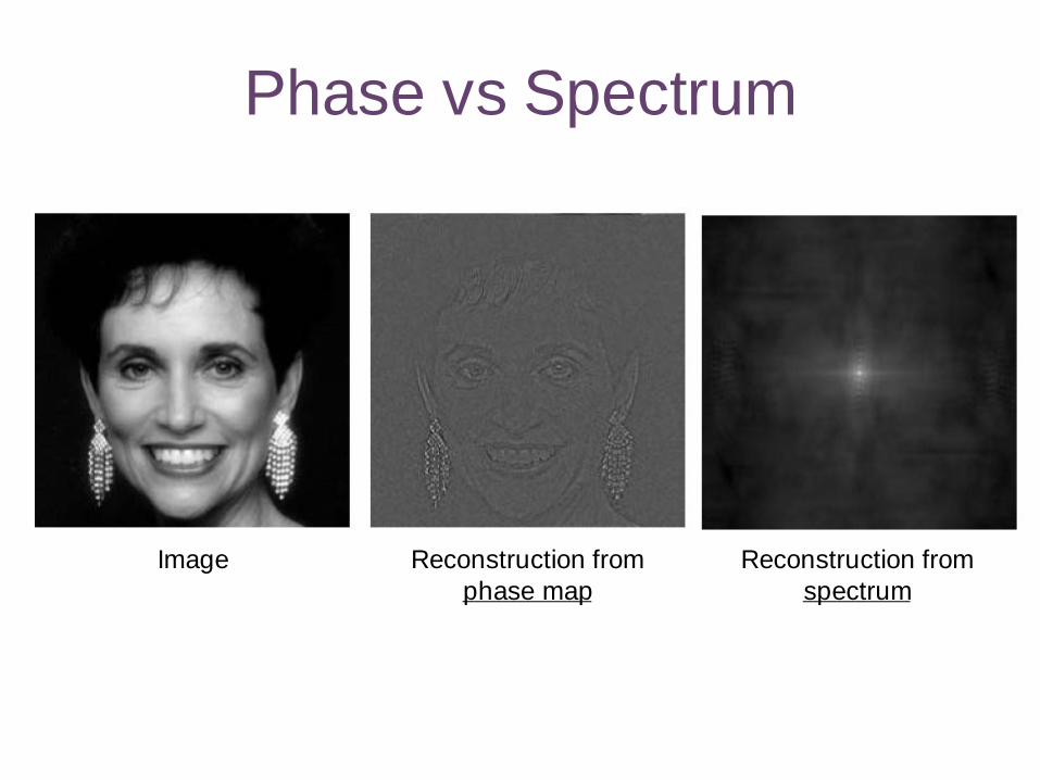
Phase vs Spectrum
Image Reconstruction from
phase map
Reconstruction from
spectrum
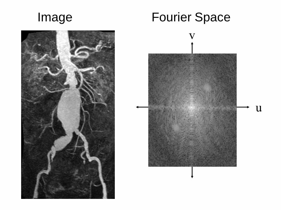
u
v
Image Fourier Space
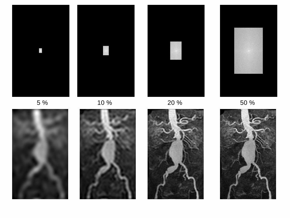
10 % 5 % 20 % 50 %
Fourier Spectrum Demo
http://bigwww.epfl.ch/demo/basisfft/demo.html
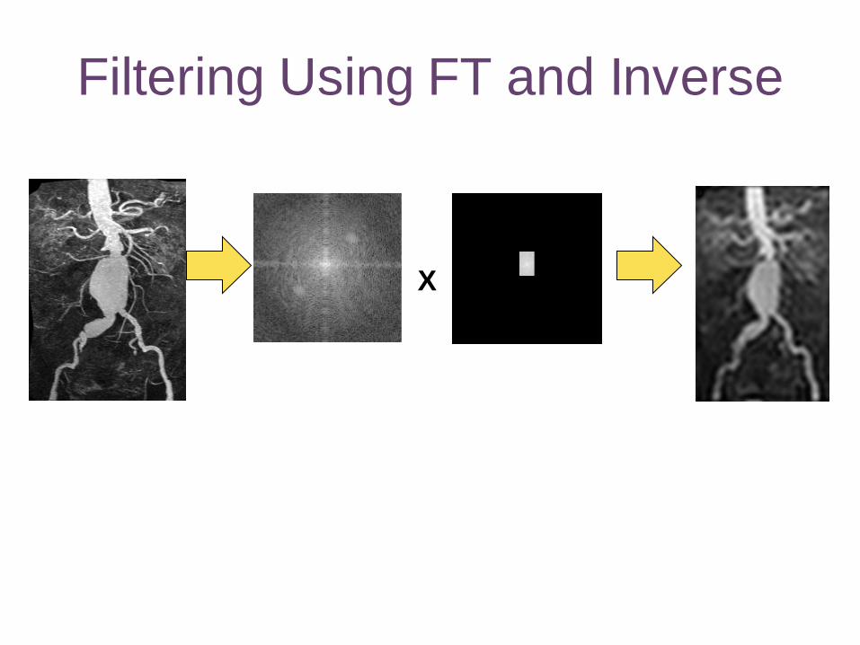
Filtering Using FT and Inverse
X
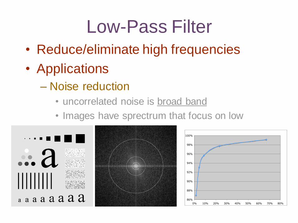
Low-Pass Filter • Reduce/eliminate high frequencies
• Applications
– Noise reduction
• uncorrelated noise is broad band
• Images have sprectrum that focus on low
frequencies
86%
88%
90%
92%
94%
96%
98%
100%
0% 10% 20% 30% 40% 50% 60% 70% 80%
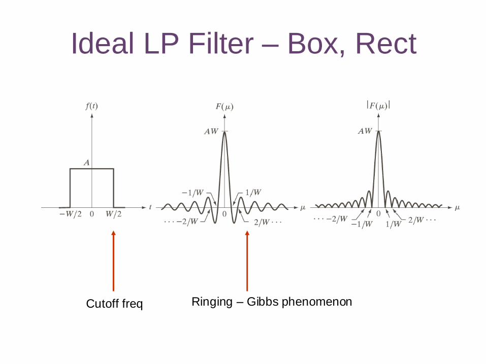
Ideal LP Filter – Box, Rect
Cutoff freq Ringing – Gibbs phenomenon
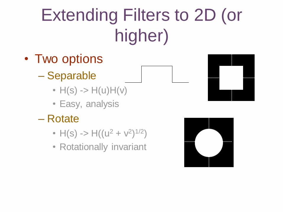
Extending Filters to 2D (or
higher)
• Two options
– Separable
• H(s) -> H(u)H(v)
• Easy, analysis
– Rotate
• H(s) -> H((u2 + v2)1/2)
• Rotationally invariant
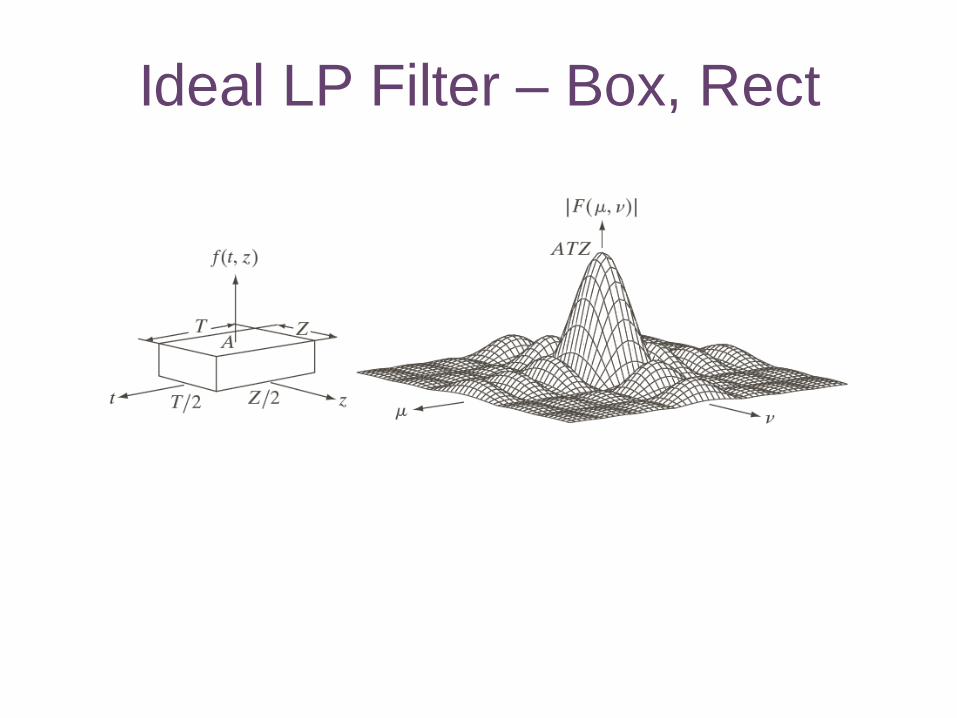
Ideal LP Filter – Box, Rect
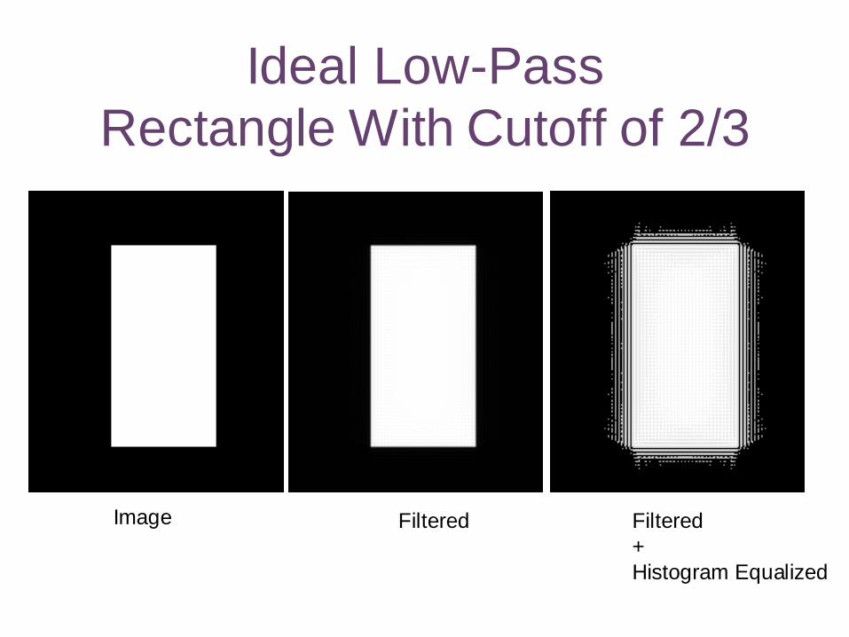
Ideal Low-Pass
Rectangle With Cutoff of 2/3
Image Filtered Filtered
+
Histogram Equalized
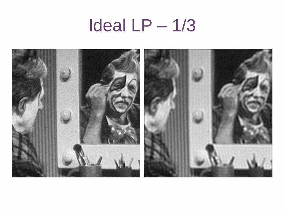
Ideal LP – 1/3
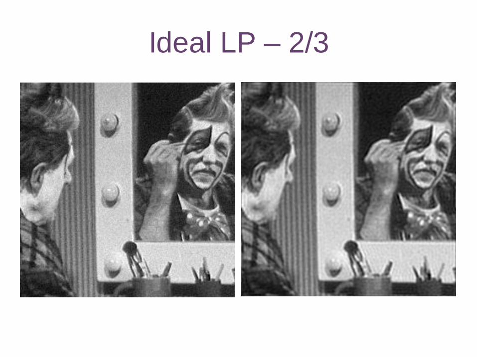
Ideal LP – 2/3
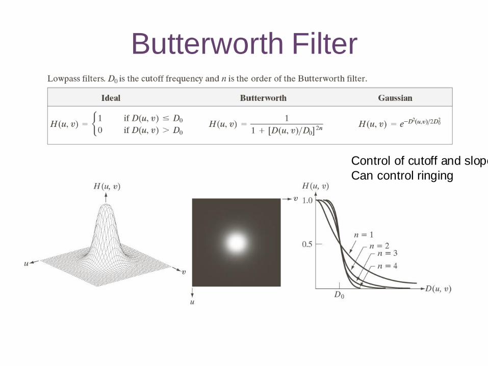
Butterworth Filter
Control of cutoff and slope
Can control ringing

Butterworth - 1/3
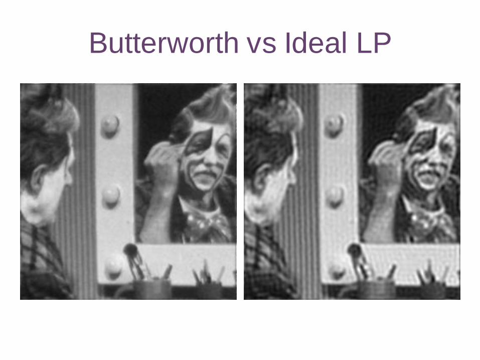
Butterworth vs Ideal LP
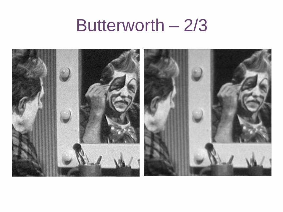
Butterworth – 2/3
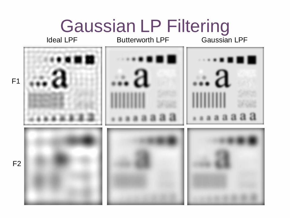
Gaussian LP Filtering Ideal LPF Butterworth LPF Gaussian LPF
F1
F2
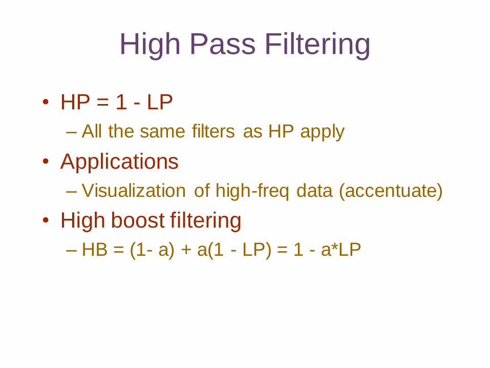
High Pass Filtering
• HP = 1 - LP
– All the same filters as HP apply
• Applications
– Visualization of high-freq data (accentuate)
• High boost filtering
– HB = (1- a) + a(1 - LP) = 1 - a*LP
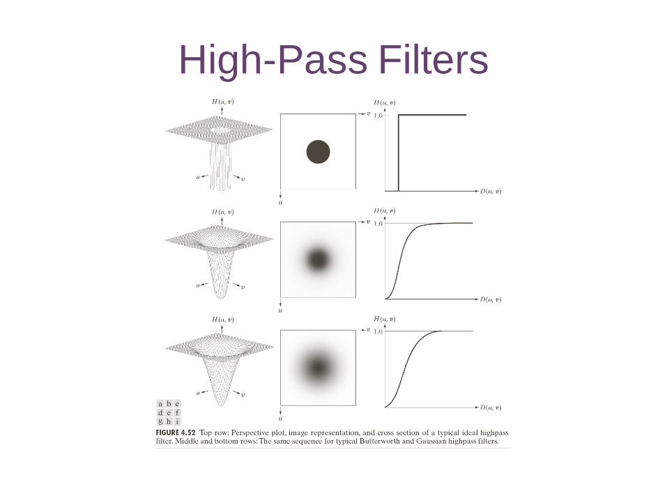
High-Pass Filters
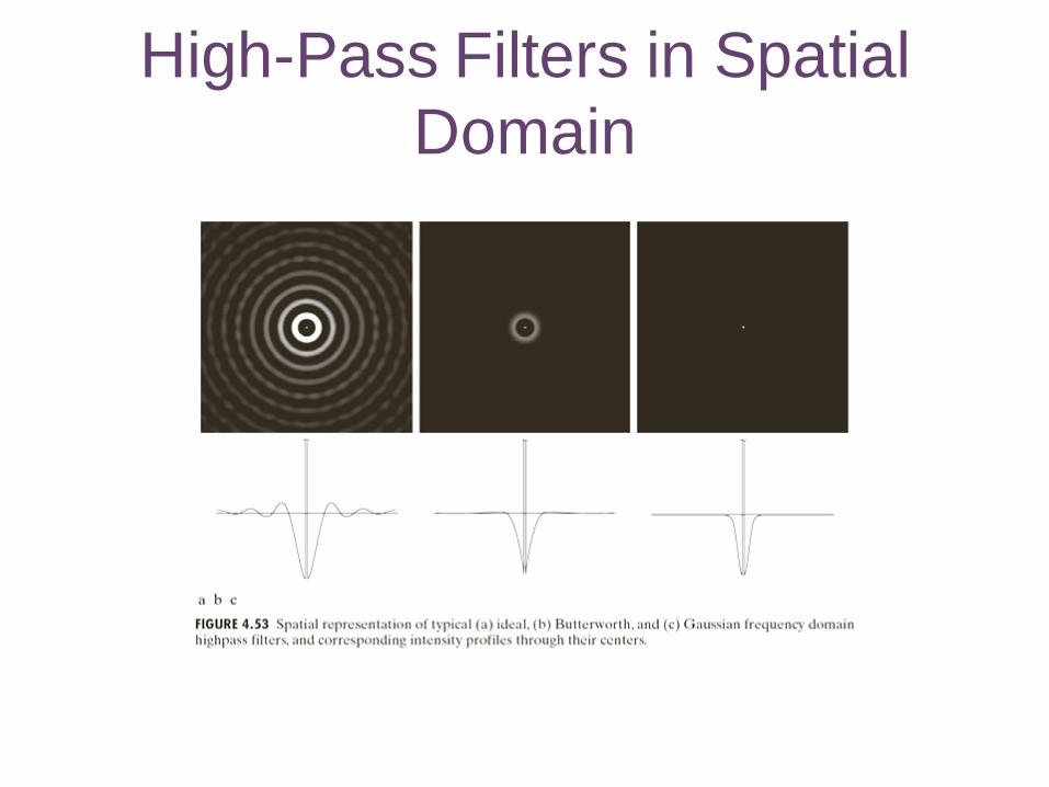
High-Pass Filters in Spatial
Domain
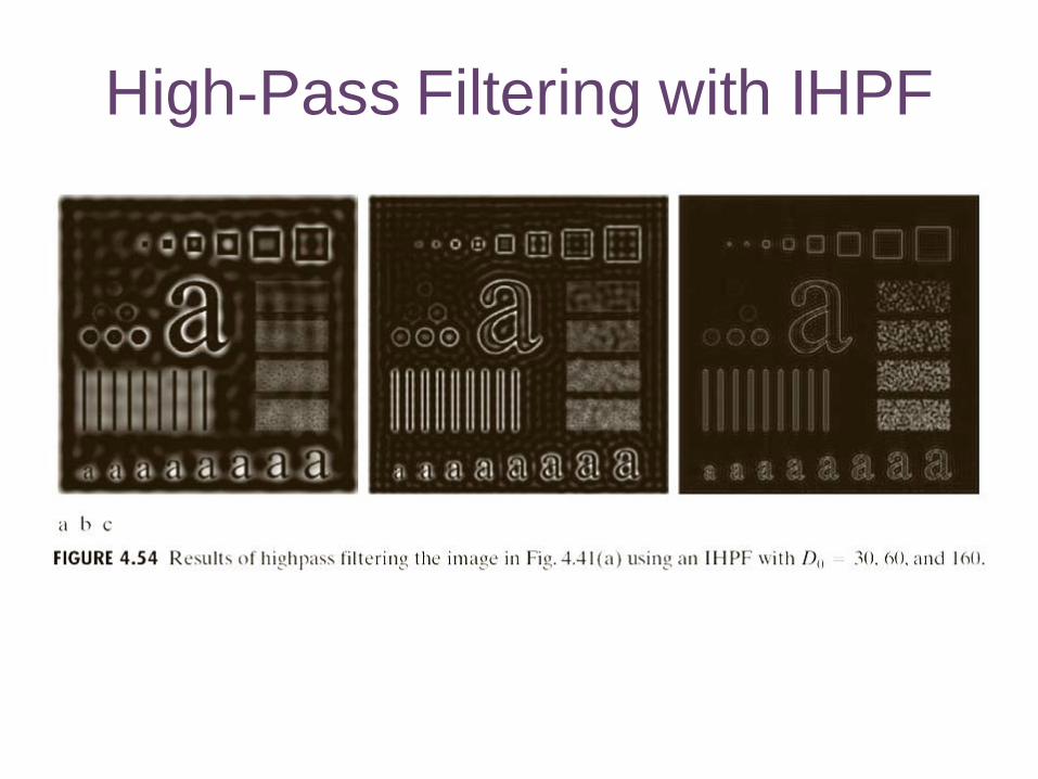
High-Pass Filtering with IHPF
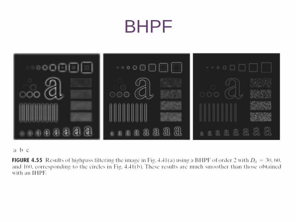
BHPF
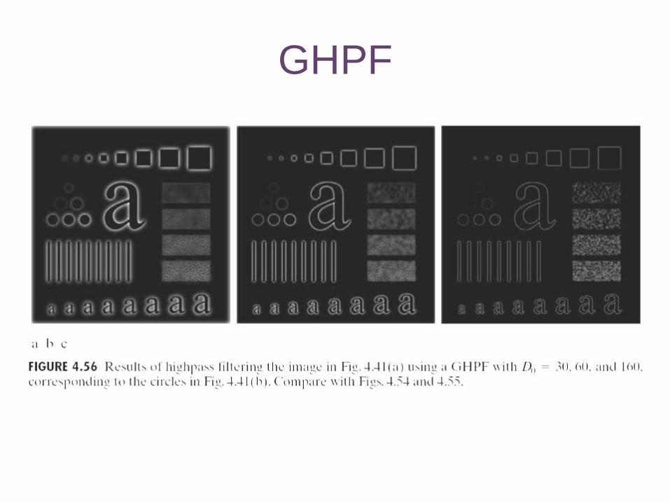
GHPF
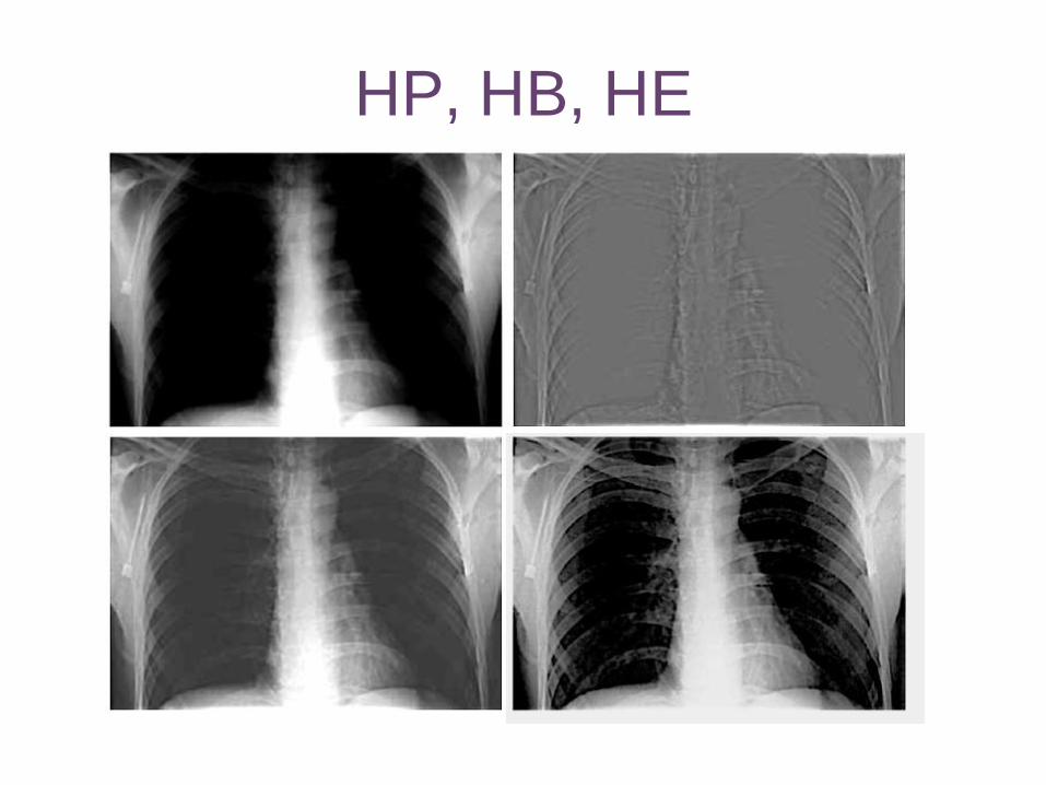
HP, HB, HE
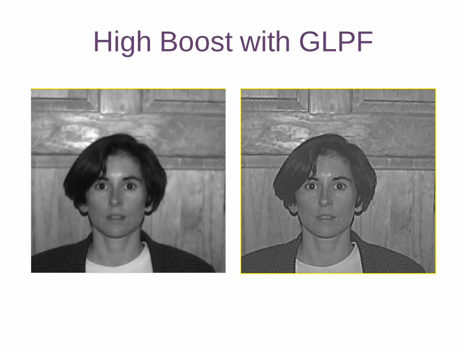
High Boost with GLPF
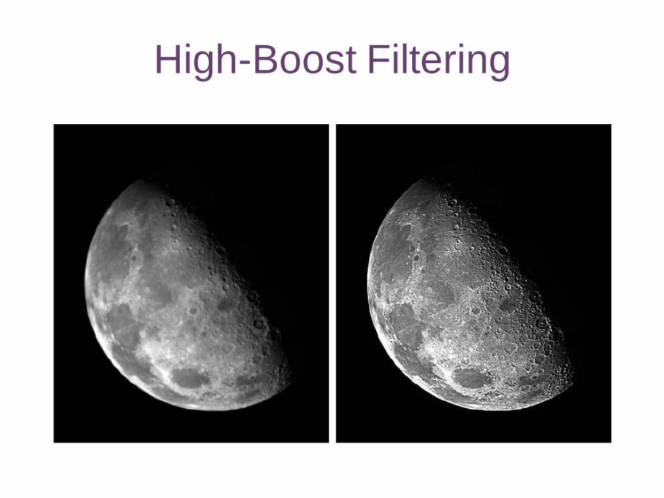
High-Boost Filtering
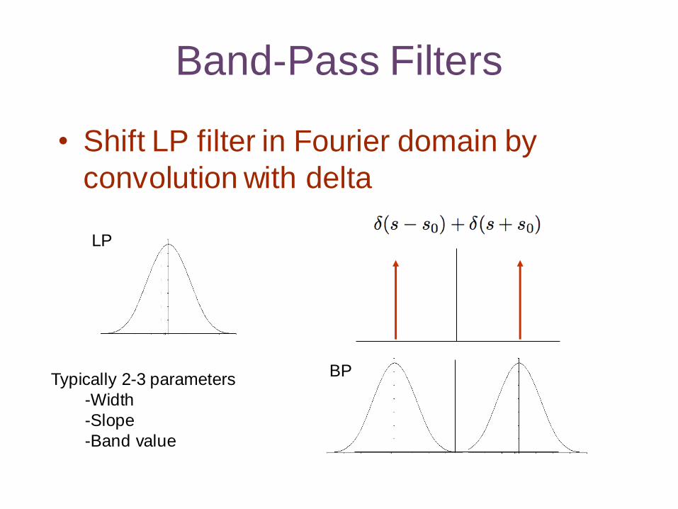
Band-Pass Filters
• Shift LP filter in Fourier domain by
convolution with delta
LP
BP Typically 2-3 parameters
-Width
-Slope
-Band value

Band Pass - Two Dimensions
• Two strategies
– Rotate
• Radially symmetric
– Translate in 2D
• Oriented filters
• Note:
– Convolution with delta-pair in FD is
multiplication with cosine in spatial domain
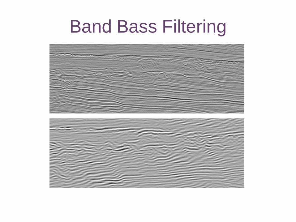
Band Bass Filtering
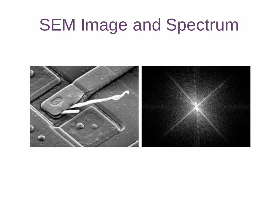
SEM Image and Spectrum
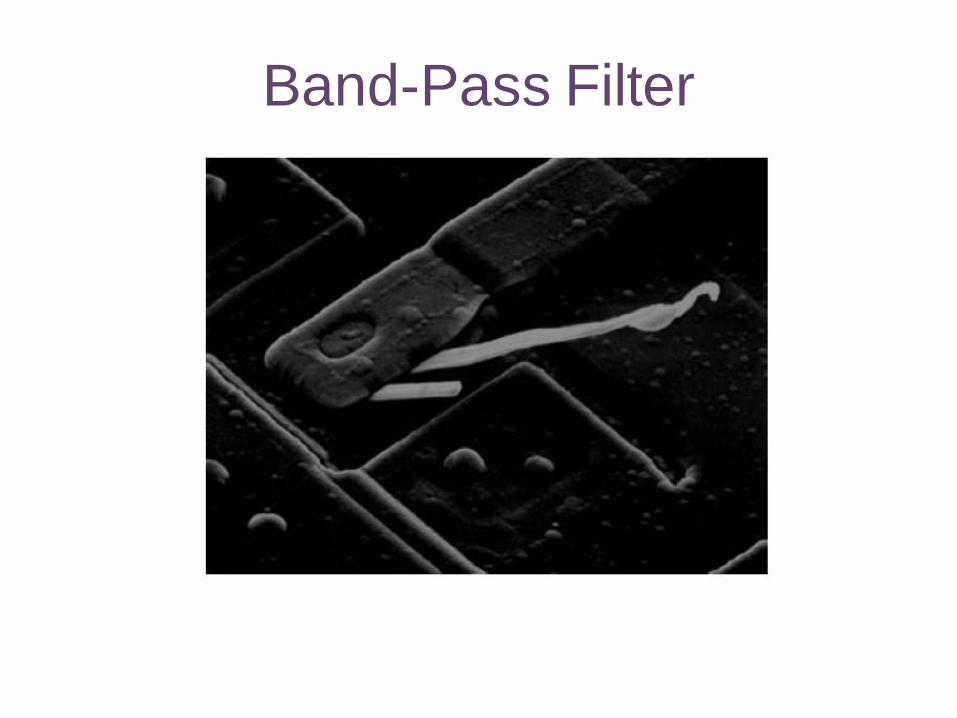
Band-Pass Filter
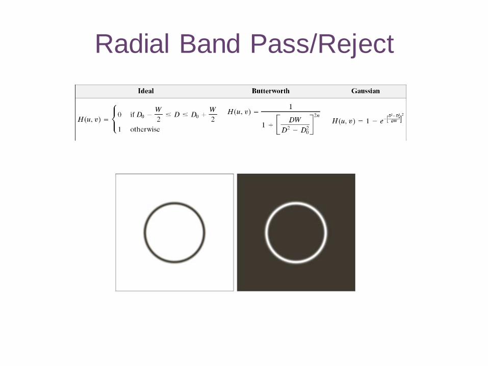
Radial Band Pass/Reject
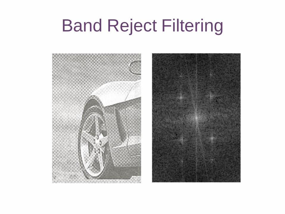
Band Reject Filtering
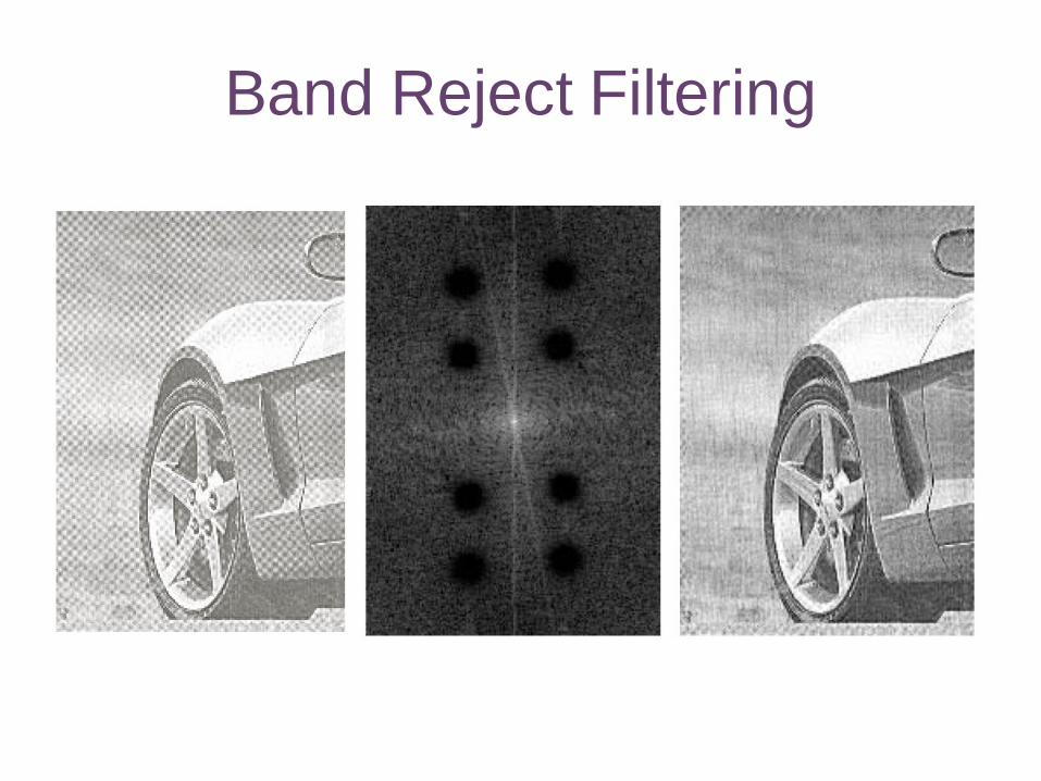
Band Reject Filtering
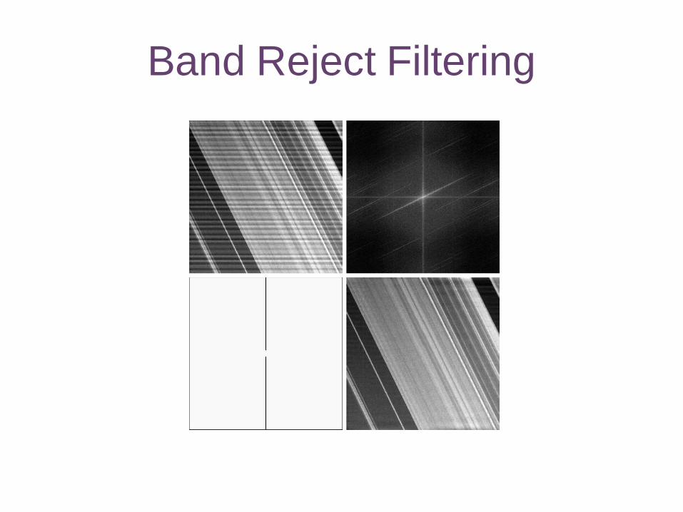
Band Reject Filtering

Aliasing
Discrete Sampling and
Aliasing • Digital signals and images are discrete
representations of the real world
– Which is continuous
• What happens to signals/images when we
sample them?
– Can we quantify the effects?
– Can we understand the artifacts and can we limit
them?
– Can we reconstruct the original image from the
discrete data?
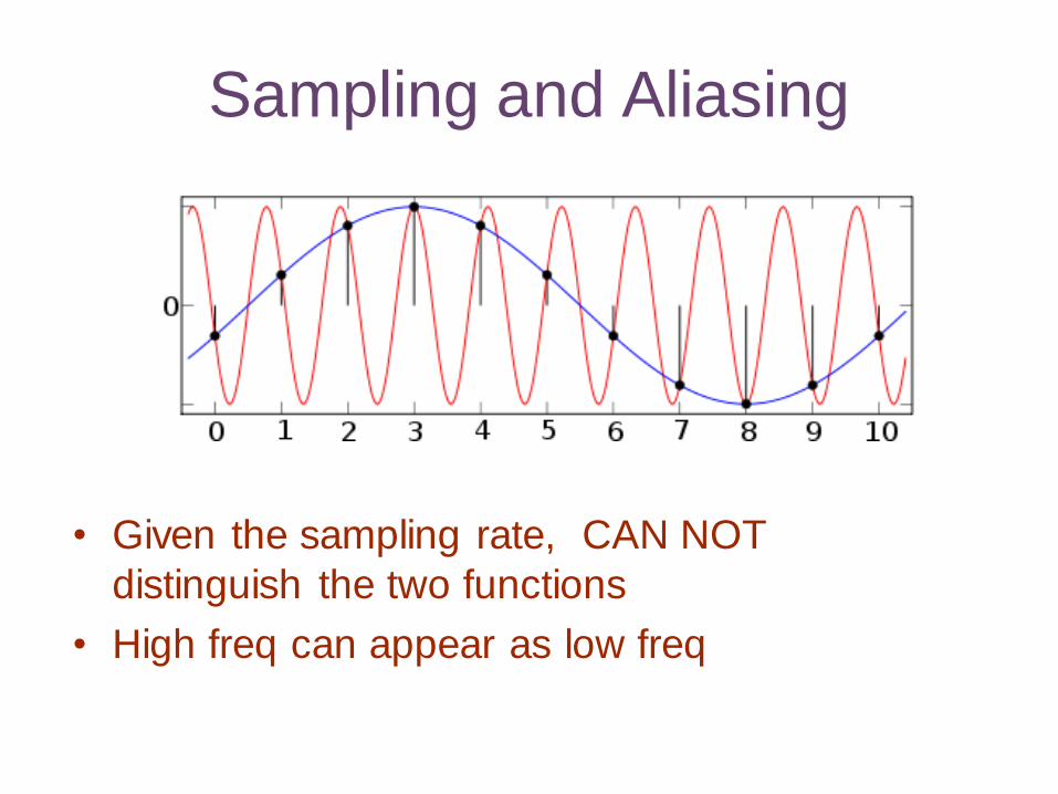
Sampling and Aliasing
• Given the sampling rate, CAN NOT
distinguish the two functions
• High freq can appear as low freq
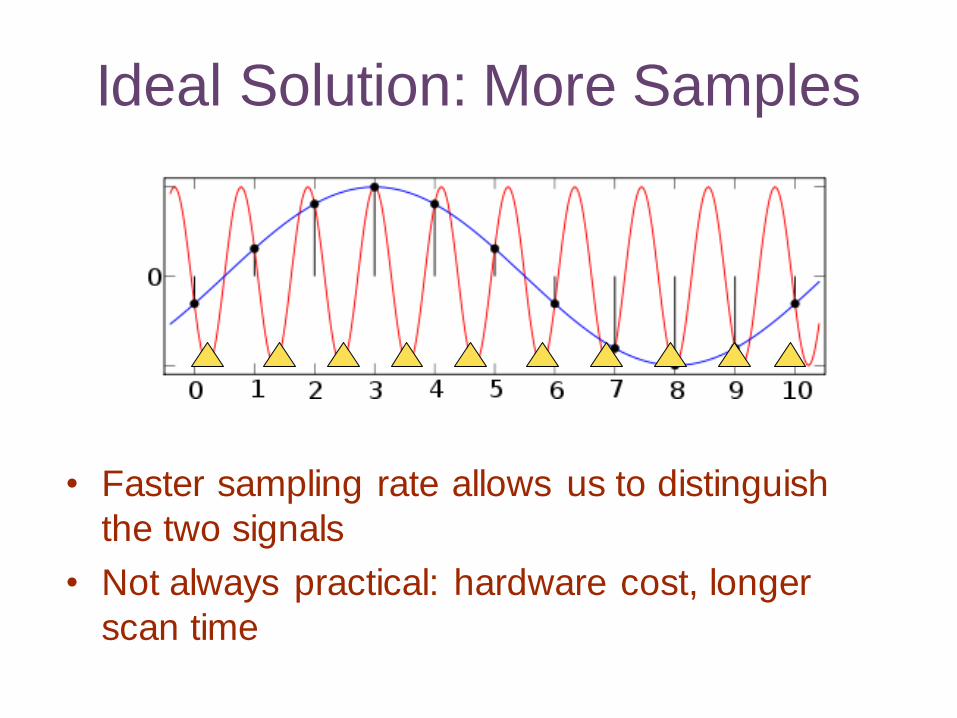
Ideal Solution: More Samples
• Faster sampling rate allows us to distinguish
the two signals
• Not always practical: hardware cost, longer
scan time
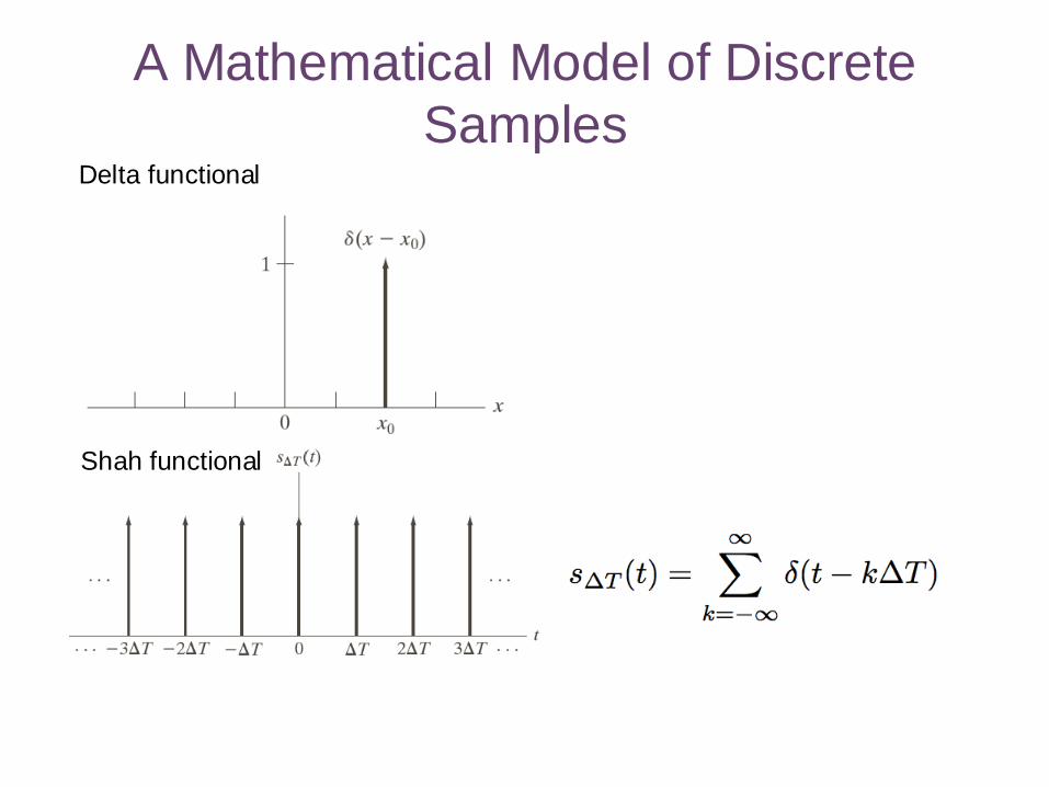
A Mathematical Model of Discrete
Samples Delta functional
Shah functional

A Mathematical Model of Discrete
Samples
Discrete signal
Samples from continuous function
Representation as a function of t
• Multiplication of f(t) with Shah
• Goal
– To be able to do a continuous Fourier
transform on a signal before and after
sampling
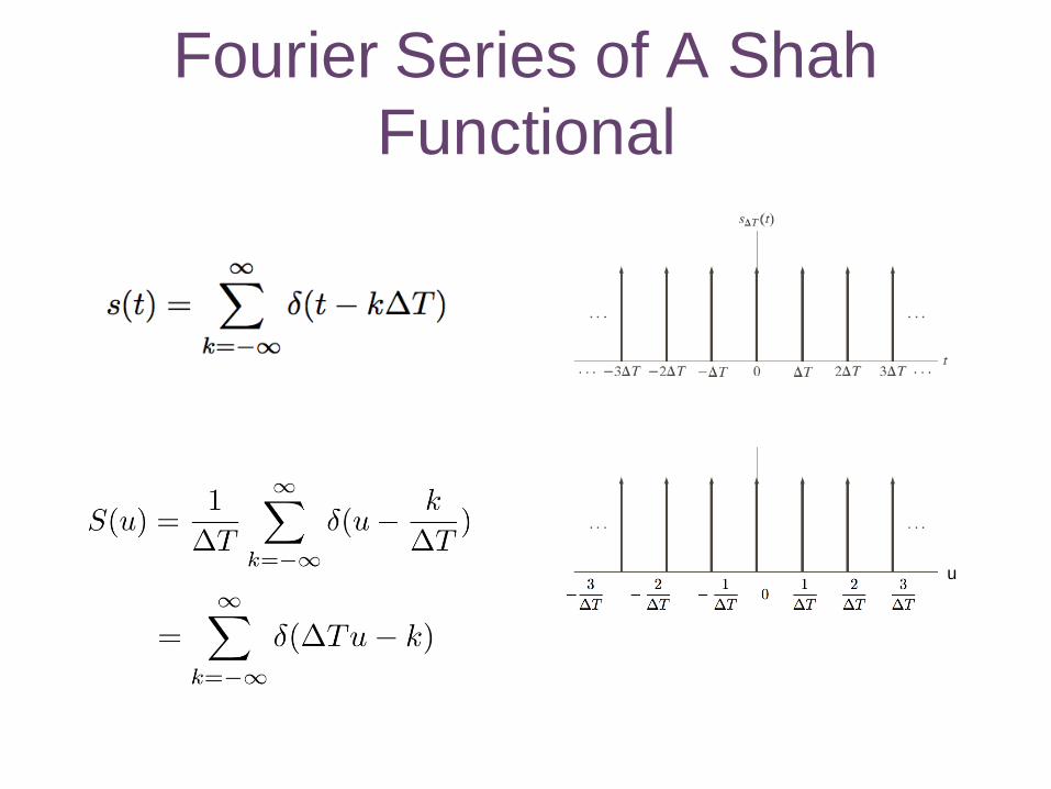
Fourier Series of A Shah
Functional
u
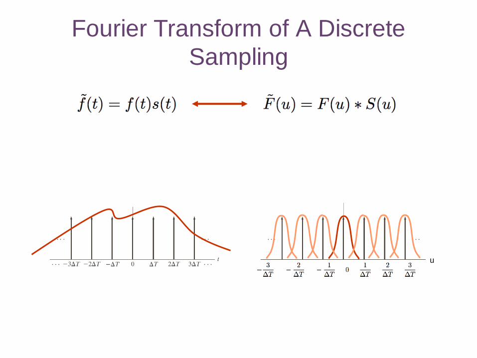
Fourier Transform of A Discrete
Sampling
u
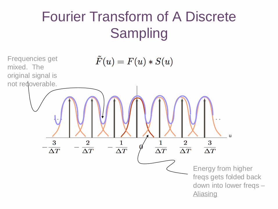
Fourier Transform of A Discrete
Sampling
u
Energy from higher
freqs gets folded back
down into lower freqs –
Aliasing
Frequencies get
mixed. The
original signal is
not recoverable.
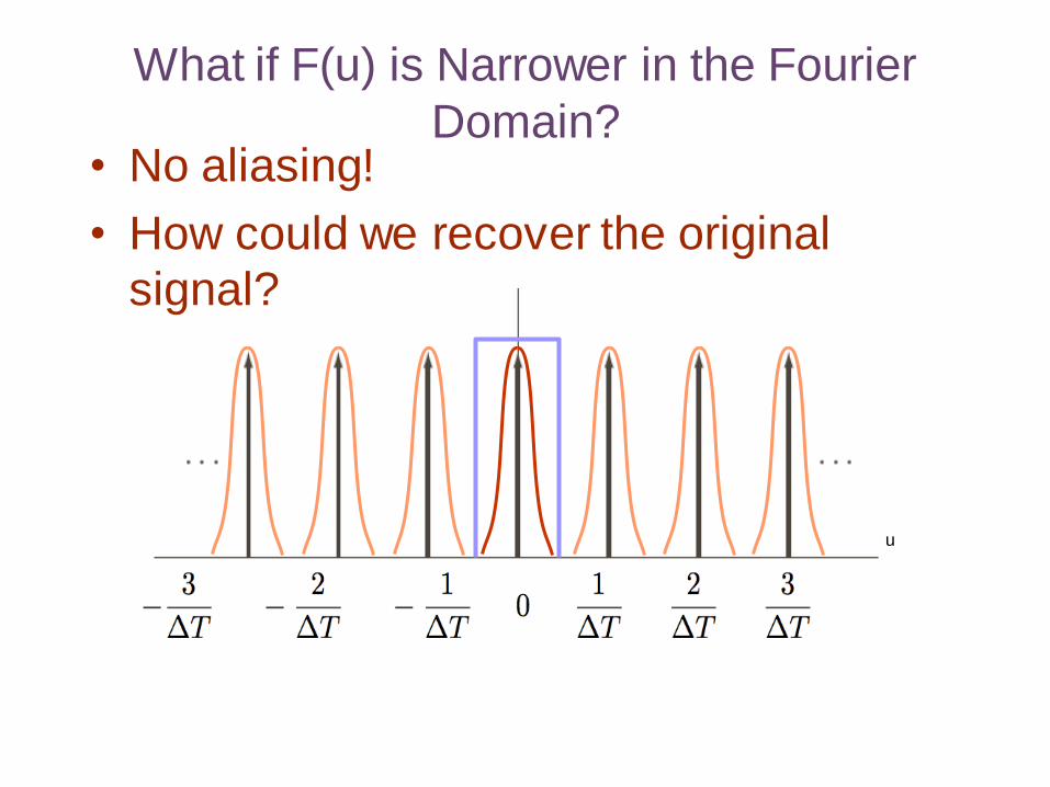
What if F(u) is Narrower in the Fourier
Domain?
u
• No aliasing!
• How could we recover the original
signal?
What Comes Out of This
Model
• Sampling criterion for complete
recovery
• An understanding of the effects of
sampling
– Aliasing and how to avoid it
• Reconstruction of signals from discrete
samples
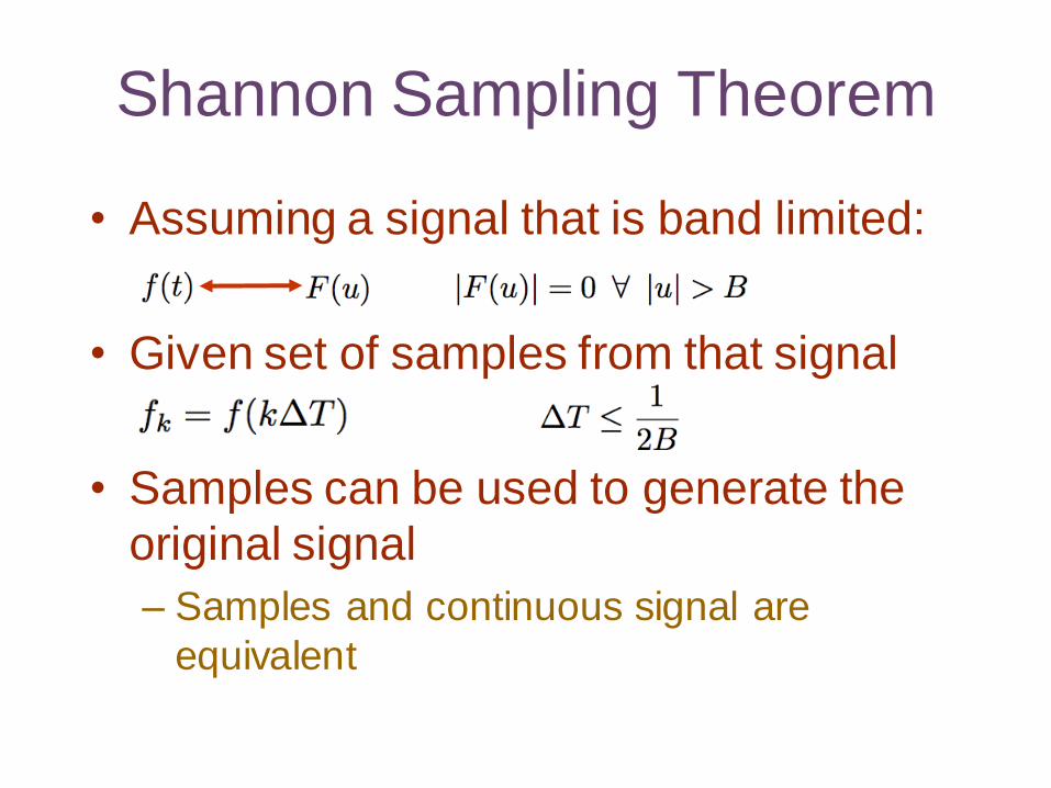
Shannon Sampling Theorem
• Assuming a signal that is band limited:
• Given set of samples from that signal
• Samples can be used to generate the
original signal
– Samples and continuous signal are
equivalent
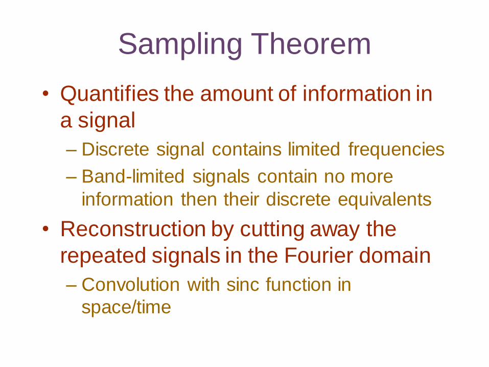
Sampling Theorem
• Quantifies the amount of information in
a signal
– Discrete signal contains limited frequencies
– Band-limited signals contain no more
information then their discrete equivalents
• Reconstruction by cutting away the
repeated signals in the Fourier domain
– Convolution with sinc function in
space/time
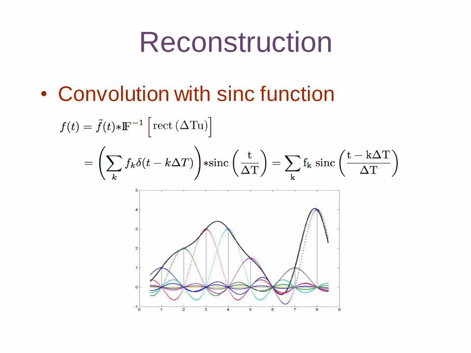
Reconstruction
• Convolution with sinc function
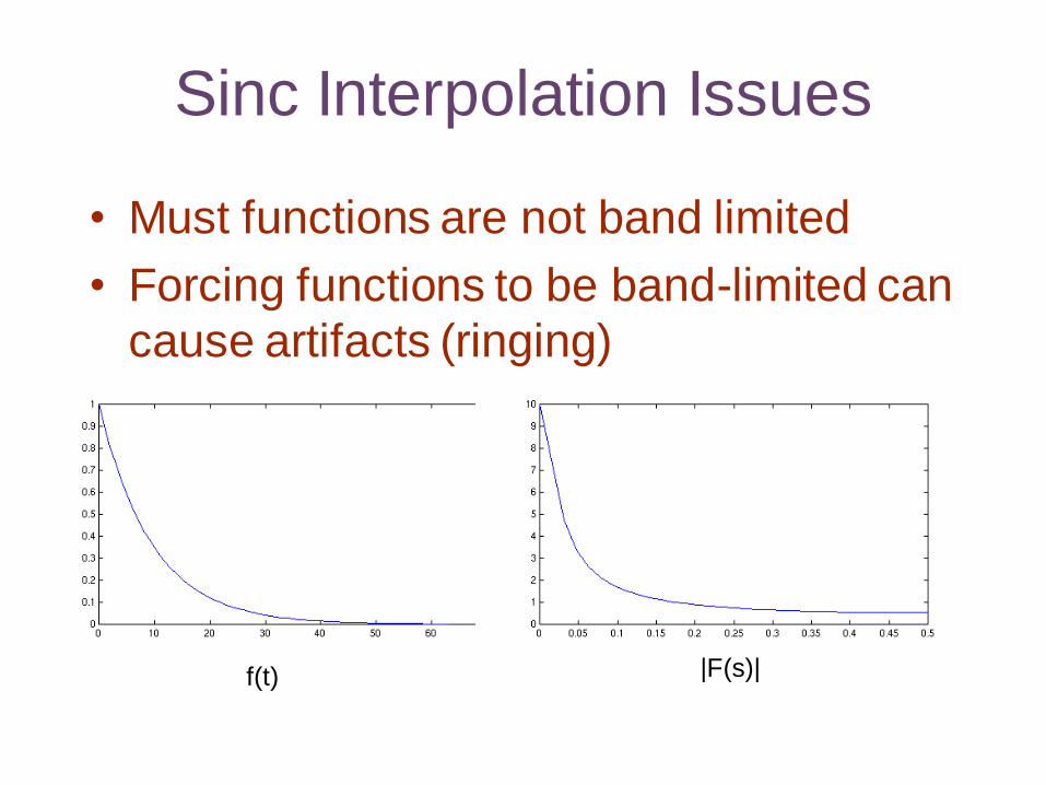
Sinc Interpolation Issues
• Must functions are not band limited
• Forcing functions to be band-limited can
cause artifacts (ringing)
f(t) |F(s)|
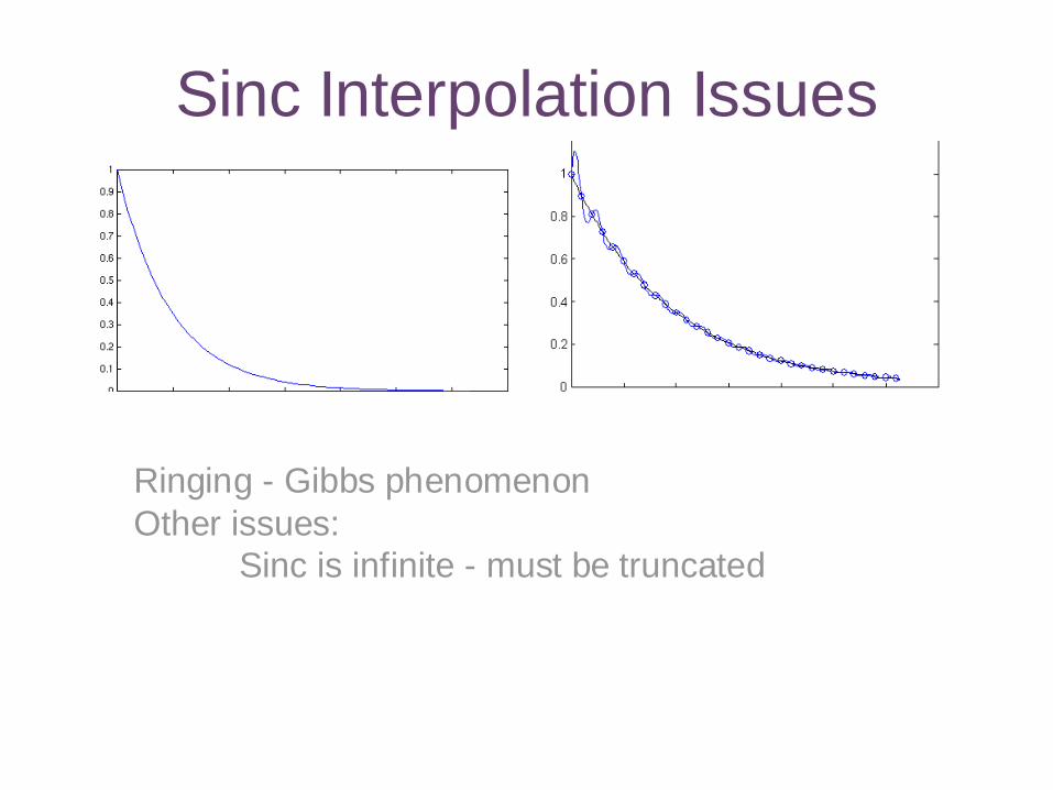
Sinc Interpolation Issues
Ringing - Gibbs phenomenon
Other issues:
Sinc is infinite - must be truncated
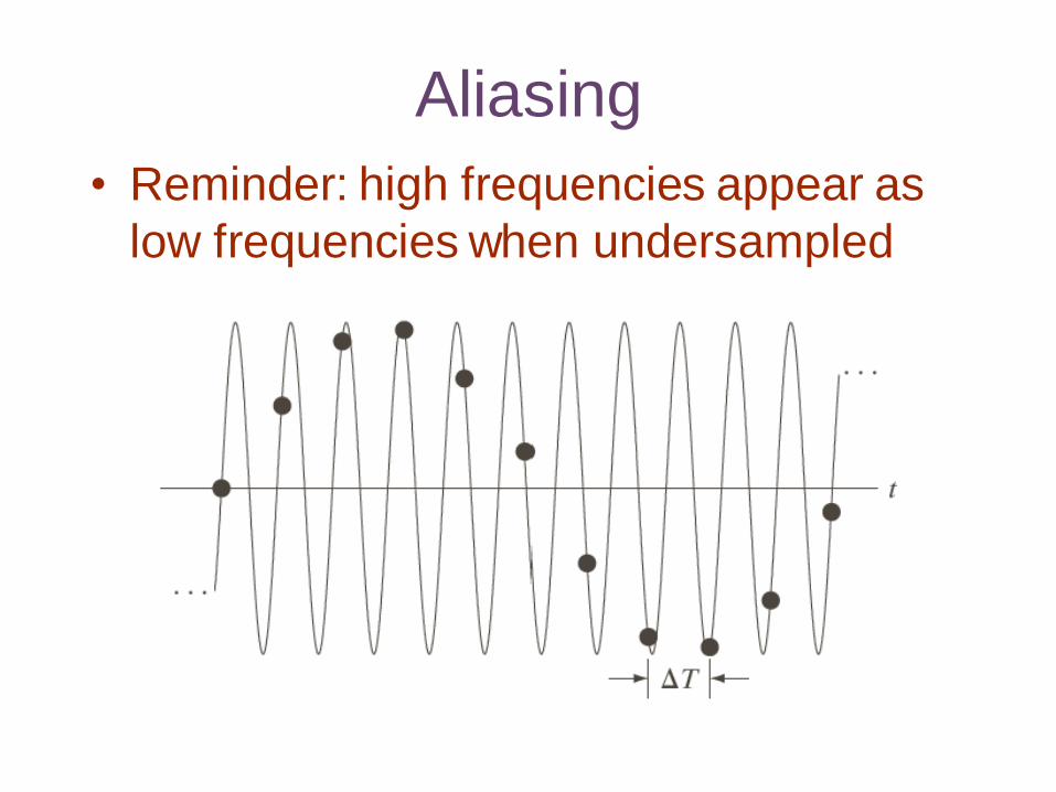
Aliasing
• Reminder: high frequencies appear as
low frequencies when undersampled
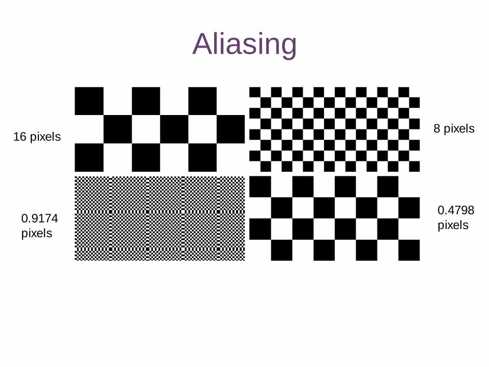
Aliasing
16 pixels 8 pixels
0.9174
pixels
0.4798
pixels
Aliasing
Aliasing in digital videos
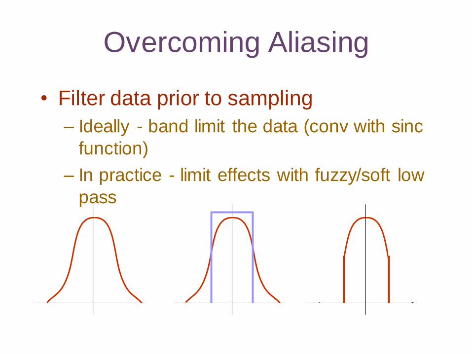
Overcoming Aliasing
• Filter data prior to sampling
– Ideally - band limit the data (conv with sinc
function)
– In practice - limit effects with fuzzy/soft low
pass
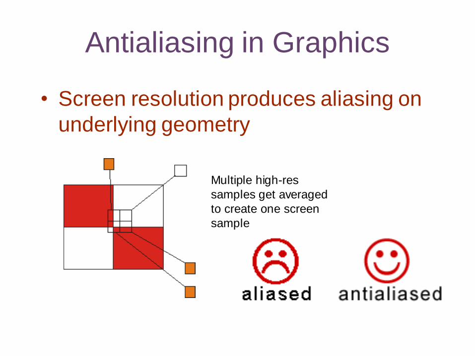
Antialiasing in Graphics
• Screen resolution produces aliasing on
underlying geometry
Multiple high-res
samples get averaged
to create one screen
sample
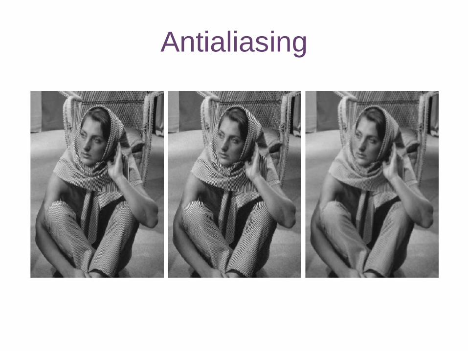
Antialiasing
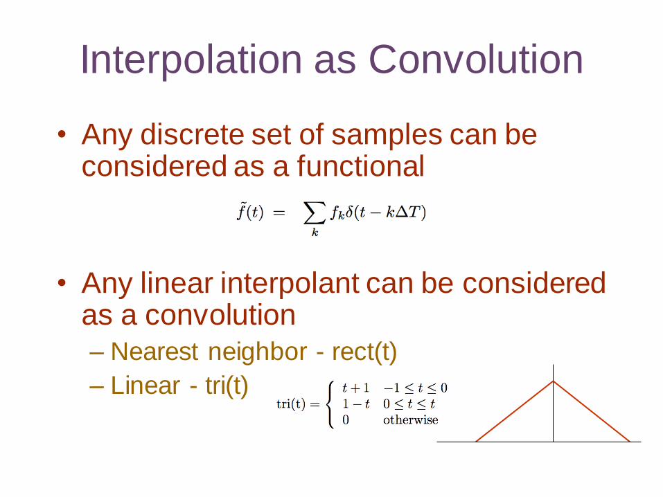
Interpolation as Convolution
• Any discrete set of samples can be considered as a functional
• Any linear interpolant can be considered as a convolution
– Nearest neighbor - rect(t)
– Linear - tri(t)
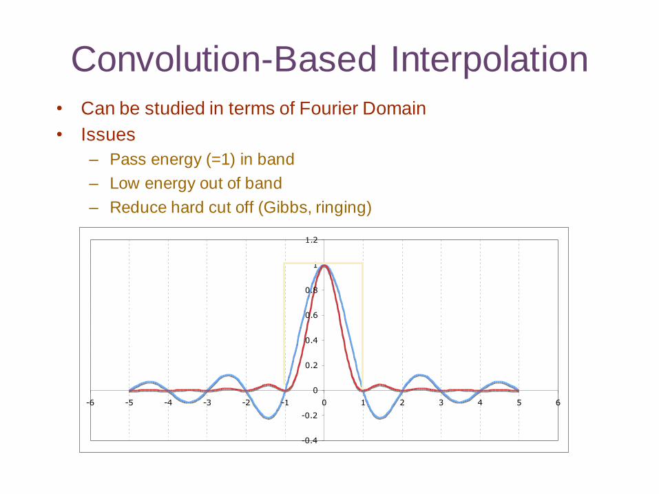
Convolution-Based Interpolation
• Can be studied in terms of Fourier Domain
• Issues
– Pass energy (=1) in band
– Low energy out of band
– Reduce hard cut off (Gibbs, ringing)
-0.4
-0.2
0
0.2
0.4
0.6
0.8
1
1.2
-6 -5 -4 -3 -2 -1 0 1 2 3 4 5 6
Fast Fourier Transform
With slides from Richard
Stern, CMU
DFT
• Ordinary DFT is O(N2)
• DFT is slow for large images
• Exploit periodicity and symmetricity
• Fast FT is O(N log N)
• FFT can be faster than convolution
Fast Fourier Transform
• Divide and conquer algorithm
• Gauss ~1805
• Cooley & Tukey 1965
• For N = 2K
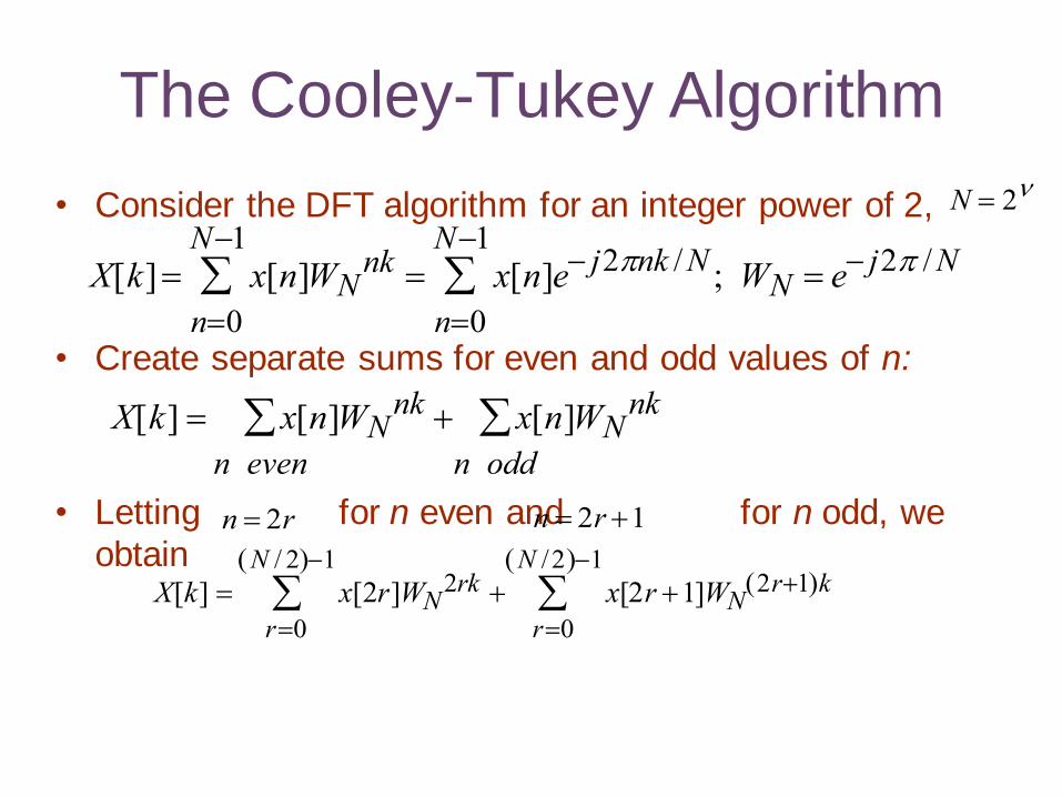
The Cooley-Tukey Algorithm
• Consider the DFT algorithm for an integer power of 2,
• Create separate sums for even and odd values of n:
• Letting for n even and for n odd, we
obtain
N 2
X[k]
n0
N1
x[n]WNnk
n0
N1
x[n]e j2nk /N ; WN e j2 /N
X[k] x[n]WNnk
n even
x[n]WNnk
n odd
n 2r n 2r 1
X[k] x[2r]WN2rk
r0
N / 2 1
x[2r 1]WN2r1 k
r0
N /2 1
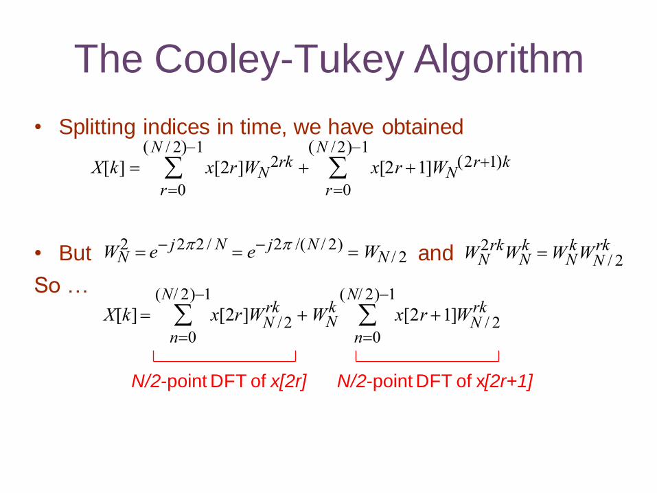
The Cooley-Tukey Algorithm
• Splitting indices in time, we have obtained
• But and
So …
N/2-point DFT of x[2r] N/2-point DFT of x[2r+1]
X[k] x[2r]WN2rk
r0
N / 2 1
x[2r 1]WN2r1 k
r0
N /2 1
WN2 e j22 / N e j2 /(N / 2) WN / 2 WN
2rkWNk WN
kWN / 2rk
X[k]
n0
(N/ 2)1
x[2r]WN /2rk WN
k
n0
(N/ 2)1
x[2r 1]WN / 2rk
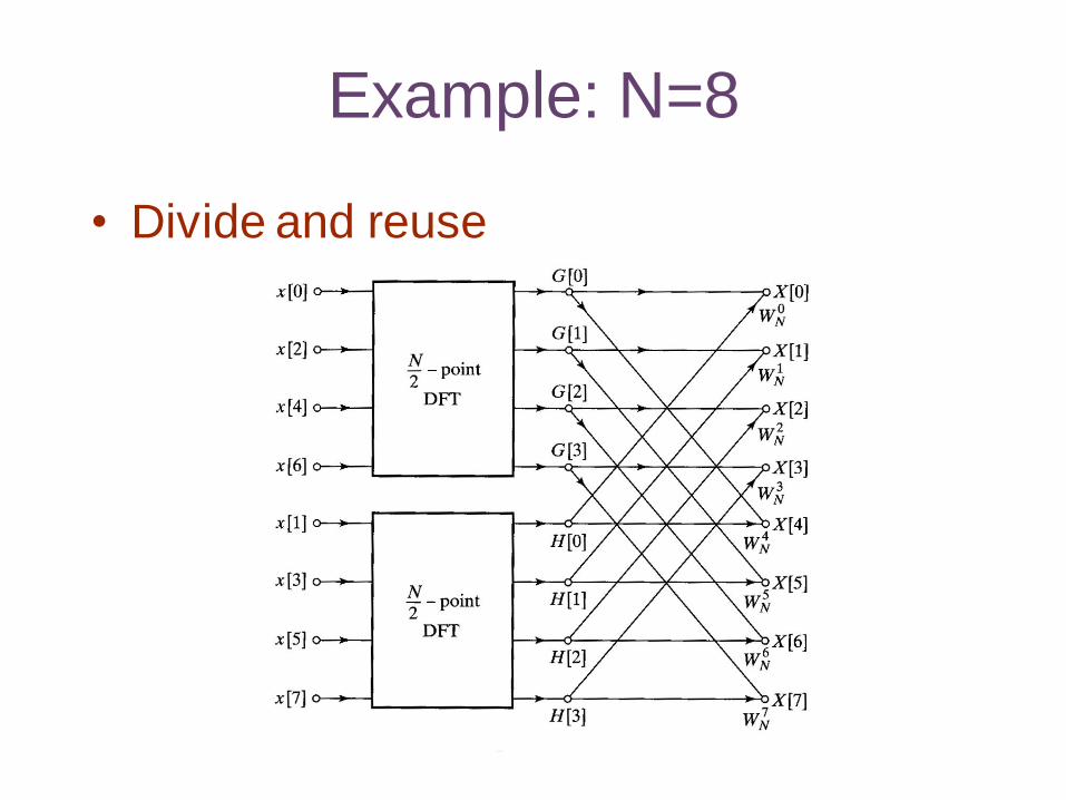
Example: N=8
• Divide and reuse
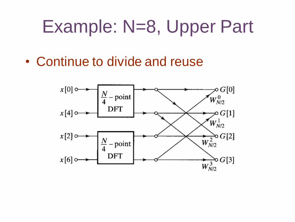
Example: N=8, Upper Part
• Continue to divide and reuse
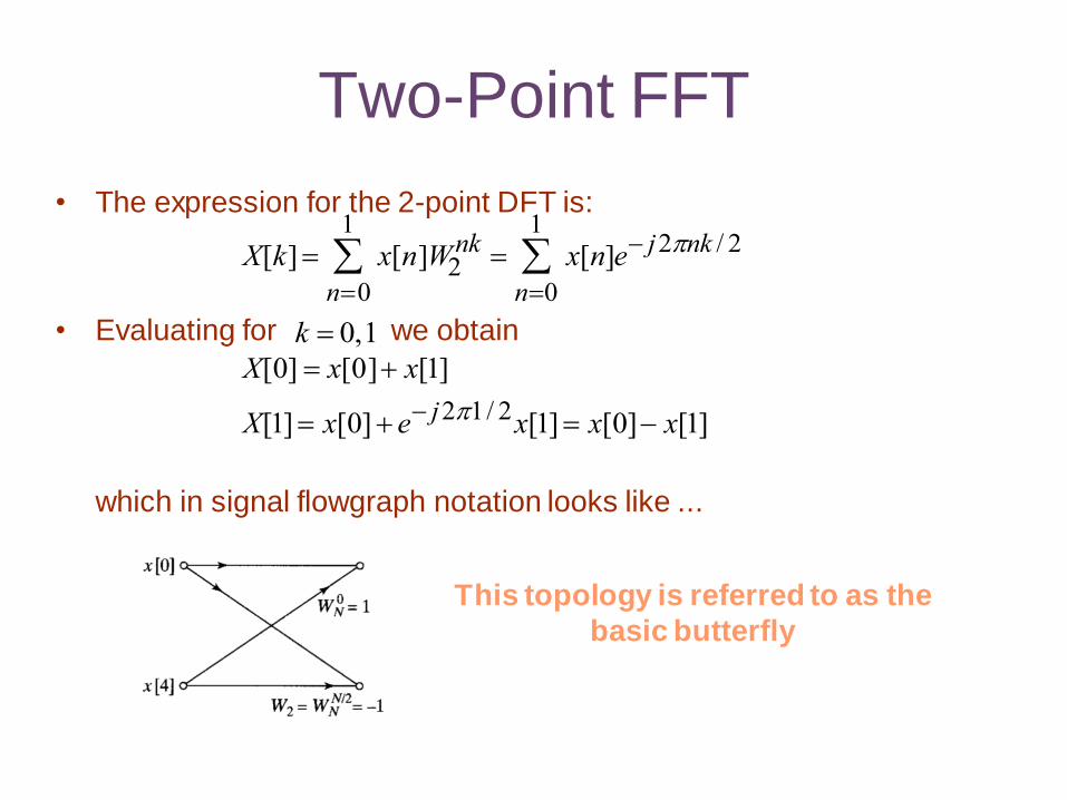
Two-Point FFT
• The expression for the 2-point DFT is:
• Evaluating for we obtain
which in signal flowgraph notation looks like ...
X[k]
n0
1
x[n]W2nk
n0
1
x[n]e j2nk / 2
k 0,1
X[0] x[0] x[1]
X[1] x[0] e j21/ 2x[1] x[0] x[1]
This topology is referred to as the
basic butterfly
Modern FFT
• FFTW
http://www.fftw.org/