Embed Size (px)
Citation preview

Undergraduate Colloquium:
Fractals, Self-similarity and Hausdorff Dimension
Andrejs Treibergs
University of Utah
Wednesday, August 31, 2016

2. USAC Lecture on Fractals
The URL for these Beamer Slides: “Fractals: self similar fractionaldimensional sets”
http://www.math.utah.edu/~treiberg/FractalSlides.pdf
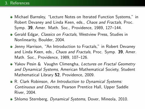
3. References
Michael Barnsley, “Lecture Notes on Iterated Function Systems,” inRobert Devaney and Linda Keen, eds., Chaos and Fractals, Proc.Symp. 39, Amer. Math. Soc., Providence, 1989, 127–144.
Gerald Edgar, Classics on Fractals, Westview Press, Studies inNonlinearity, Boulder, 2004.
Jenny Harrison, “An Introduction to Fractals,” in Robert Devaneyand Linda Keen, eds., Chaos and Fractals, Proc. Symp. 39, Amer.Math. Soc., Providence, 1989, 107–126.
Yakov Pesin & Vaughn Climengha, Lectures on Fractal Geometryand Dynamical Systems, American Mathematical Society, StudentMathematical Library 52, Providence, 2009.
R. Clark Robinson, An Introduction to Dynamical Systems:Continuous and Discrete, Pearson Prentice Hall, Upper SaddleRiver, 2004.
Shlomo Sternberg, Dynamical Systems, Dover, Mineola, 2010.

4. Outline.
Fractals
Middle Thirds Cantor Set Example
Attractor of Iterated Function System
Cantor Set as Attractor of Iterated Function System.Contraction MapsComplete Metric Space of Compact Sets with Hausdorff DistanceHutchnson’s Theorem on Attractors of Contracting IFSExamples: Unequal Scaling Cantor Set, Sierpinski Gasket, von KochSnowflake, Barnsley Fern, Minkowski Curve, Peano Curve, LevyDragon
Hausdorff Measure and Dimension
Dimension of Cantor Set by Covering by Intervals
Similarity Dimension
Similarity Dimension of Cantor SetSimilarity Dimension for IFS of Similarity TransformationsMoran’s TheoremSimilarity Dimensions of Examples
Kiesswetter’s IFS Construction of Nowhere Differentiable Function

5. Fractal. Cantor Set.
A fractal is a set with fractional dimension. A fractal need not beself-similar. In this lecture we construct self-similar sets of fractionaldimension. The most basic fractal is the Middle Thirds Cantor Set. Onestarts from an interval I1 = [0, 1] and at each successive stage, removesthe middle third of the intervals remaining in the set.
I2 =
[0,
1
3
]∪[
2
3, 1
]I3 =
[0,
1
9
]∪[
2
9,
1
3
]∪[
2
3,
7
9
]∪[
8
9, 1
]I4 =
[0,
1
27
]∪[
2
27,
1
9
]∪[
2
9,
7
27
]∪[
8
27,
1
3
]∪[
2
3,
19
27
]∪[
20
27,
7
9
]∪[
8
27,
25
27
]∪[
26
27, 1
]· · ·
Then the Cantor Set is the limit C =⋂∞
n=1 In.

6. Picture of Cantor Sets
Figure: The sequence In approximating the middle thirds Cantor Set.

7. “Butterfly” Attractor of Lorenz Equations.
“Butterfly” ODE limit set is a non self-similar fractal 1 < dimH(A) < 2

8. Cantor Set as the Attractor of an Iterated Function System
The Cantor Set may be constructed using Iterated Function Systems.The IFS is given by two maps on the line, F = `, r, where
`(x) =x
3; r(x) =
x + 2
3.
` and r make two shrunken copies of the original interval located at theleft and right ends. Define the induced union map taking compact setsA ⊂ R to new compact sets consisting of both shrunken copies
F(A) = `(A) ∪ r(A)
where `(A) = `(x) : x ∈ A. Consider the dynamical system of iteratingthe maps. We get the Cantor Set as its its attractor (limit)
I2 = F(I1), I3 = F(I2), . . . , C = limn→∞
Fn(I1)
where we define F F(A) = F(F(A)) and
Fn(A) =
n times︷ ︸︸ ︷F F · · · F(A)

9. Metric Spaces
Why does the sequence of sets converge? Let us put the structure of ametric space on the space of compact sets and do a little analysis.
For example, the distance function d on Euclidean Space X = En is
d(x , y) = ‖x − y‖ =
√√√√ n∑i=1
(xi − yi )2.
Euclidean Space has the structure of a metric space, namely, for allx , y , z ∈ X we have
d(x , x) = 0, d(x , y) = d(y , x),
d(x , z) ≤ d(x , y) + d(y , z) triangle inequality(which implies d(x , x) ≥ 0),
d(x , y) = 0 implies x = y .

10. Complete Metric Spaces
xi ⊂ En is a Cauchy Sequence if for every ε > 0 there is an N such that
d(xi , xj) < ε whenever i , j ≥ N.
Euclidean Space is a complete metric space because all Cauchy Sequencesconverge. Namely, if xi is a Cauchy Sequence, then there is z ∈ En
such that xi → z as i →∞, i.e., for all ε > 0, there is N > 0 such that
d(xi , z) < ε whenever i > N.
A set K is compact if every sequence xi ⊂ K has a subsequence thatconverges to a point of K . In Euclidean Space, K ∈ En is compact if andonly if it is closed and bounded (Heine Borel Theorem).
Surprisingly, the space K(En) of all compact sets En and can be endowedwith the structure of a complete metric space under the HausdorffMetric.

11. ε-Collar of a Set
Figure: ε-Collar of A.
Let K(En) denote the nonempty compact subsets.For any A ∈ K(En) and ε ≥ 0 define the theε-collar of A to be points within ε of A
Aε = x ∈ En : d(x , y) ≤ ε for some y ∈ A.
The distance of a point x to A is
d(x ,A) = infy∈A
d(x , y).
It is zero if x ∈ A. The ε-collar may also be given
Aε = x ∈ En : d(x ,A) ≤ ε.
The infimum is achieved since A is compact. Thereis a y ∈ A so that
d(x , y) = d(x ,A).

12. Hausdorff Distance
Given compact sets A,B ∈ K(En), if we let
d(A,B) = maxx∈A
d(x ,B).
d(A,B) ≤ ε implies that A ⊂ Bε.
BUT d(A,B) MAY NOT EQUAL d(B,A) so it is not a metric. e.g.,A = x ∈ E2 : |x | ≤ 1, B = (2, 0) then d(B,A) = 1 so B ⊂ A1 butd(A,B) = 3 and A 6⊂ B1.
Hausdorff introduced
h(A,B) = maxd(A,B), d(B,A) = infε ≥ 0 : A ⊂ Bε and B ⊂ Aε
Theorem (Completeness of K(En))
K(En) with Hausdorff Distance h is a complete metric space.Furthermore, h satisfies for all A,B,C ,D ∈ K(En)
h(A ∪ B,C ∪ D) ≤ maxh(A,C ), h(B,D)

13. Proof of the Completeness Theorem for (K (En), h)
Proof. Symmetry (h(A,B) = h(B,A)) and positive definiteness(h(A,B) ≥ 0 with h(A,B) = 0⇐⇒ A = B) are obvious. To prove thetriangle inequality it suffices to show
d(A,B) ≤ d(A,C ) + d(C ,B).
This implies the triangle inequality for h:
h(A,B) = maxd(A,B), d(B,A)≤ maxd(A,C ) + d(C ,B), d(B,C ) + d(C ,A)≤ maxh(A,C ) + h(C ,B), h(B,C ) + h(C ,A)= h(A,C ) + h(C ,B).
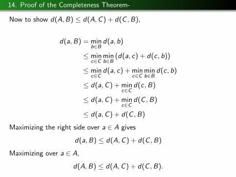
14. Proof of the Completeness Theorem-
Now to show d(A,B) ≤ d(A,C ) + d(C ,B),
d(a,B) = minb∈B
d(a, b)
≤ minc∈C
minb∈B
(d(a, c) + d(c , b))
≤ minc∈C
d(a, c) + minc∈C
minb∈B
d(c , b)
≤ d(a,C ) + minc∈C
d(c ,B)
≤ d(a,C ) + minc∈C
d(C ,B)
≤ d(a,C ) + d(C ,B)
Maximizing the right side over a ∈ A gives
d(a,B) ≤ d(A,C ) + d(C ,B)
Maximizing over a ∈ A,
d(A,B) ≤ d(A,C ) + d(C ,B).

15. Proof of the Completeness Theorem- -
Sketch of completeness argument: suppose An is a Cauchy Sequence in(K(X ), h). Define A∞ to be the set of cluster points of sequences xnwhere xn ∈ An. Thus x ∈ A∞ if and only if there is a subsequence of thistype such that xkj → x as j →∞. Since the sets form a CauchySequence, for every ε > 0 there is an R(ε) so that h(An,Am) < εwhenever m, n ≥ R(ε). In particular, Am ⊂ (An)ε for all m ≥ n ≥ R(ε) soany sequence xm ∈ Am is bounded and thus has a cluster point showingA∞ is nonempty. Limits satisfy A∞ ⊂ (An)ε for all n ≥ R(ε), hence A∞is bounded. A convergent sequence of cluster points is a cluster point, soA∞ is closed, thus A∞ is compact.To show that An ⊂ (A∞)ε whenever n ≥ R(ε), pick zn ∈ An. Fork ≥ R(ε), h(An,Ak) < ε, so there is xk ∈ Ak so d(xk , zn) < ε. Letz ∈ A∞ be a cluster point of xk. For its converging subsequenced(z , zm) = limj→∞ d(xkj , zm) ≤ ε so zm ∈ (A∞)ε.Putting the containments together shows h(Am,A∞) ≤ ε for allm ≥ R(ε), thus Am converges to A∞ in the Hausdorff metric.

16. Contraction .
A mapping f : En → En is a λ-contraction if there is a constant0 ≤ λ < 1 such that
d(f (x), f (y)) ≤ λd(x , y), for all x , y ∈ En.
Lemma
If f : En → En is a λ-contraction, then the induced map on K(En) is acontraction in the Hausdorff Metric with the same constant
h(f (A), f (B)) ≤ λh(A,B), for all A,B ∈ K(En) .
Proof. Choose A,B ∈ K(En).
d(f (A), f (B)) = maxa∈A
d(f (a), f (B)) ≤ λmaxa∈A
d(a,B) = λd(A,B).
Similarly, d(f (B), f (A)) ≤ λd(B,A). Combining,
h(f (A), f (B)) = maxd(f (A), f (B)), d(f (B), f (A))≤ λmaxd(A,B), d(B,A) = λh(A,B).

17. Hutchnson’s Lemma
Lemma (Hutchinson 1981)
Let f1, . . . , fk : En → En be an IFS of contractions with constants λk .Then the induced union map on K(En) given for A ∈ K(En) by
F(A) = f1(A) ∪ f2(A) ∪ · · · ∪ fk(A)
is a contraction with the constant λ = maxλ1, . . . , λk.
Proof. Choose A,B ∈ K(En). Since a point is closer to a union of setsthan to any one set in the union,
d(F(A),F(B)) = d(∪ki=1fi (A),∪kj=1fj(B)
)= max
1≤i≤k
d(fi (A),∪kj=1fj(B))
≤ max
1≤i≤kd(fi (A), fi (B)) ≤ max
1≤i≤kλid(A,B)) ≤ λd(A,B).
Similarly, d(F(B),F(A)) ≤ λd(B,A). Combining as beforeh(F(A),F(B)) ≤ λh(A,B).

18. Contraction Mapping Theorem
One of the ten basic facts every math major must know.
Theorem (Contraction Mapping)
Let (X , d) be a complete metric space and f : X → X be a contraction.Then there is a unique fixed point x∞ ∈ X such that f (x∞) = x∞.
In fact, x∞ may be found by iteration. Starting from any x0 ∈ X , definethe sequence x1 = f (x0), x2 = f (x1), . . . , xn+1 = f (xn), . . . . Then oneshows that the sequence converges to a unique point
x∞ = limn→∞
xn.
Applying this to iterated function systems, if F : K(En)→ K(En) is acontraction then there is a unique invariant set A∞ ∈ K(En) such thatF(A∞) = A∞. It is found as the unique attractor for the dynamicalsystem F : K(En)→ K(En). For any nonempty compact set S ,
A∞ = limn→∞
Fn(S).

19. Cantor Set with Unequal Intervals
Figure: Cantor Set with Unequal Intervals
This Cantor set is obtainedfrom IFS F = f1, f2 on Rwhere
f1(x) = .4x ,
f2(x) = .5x + .5
Each fi ’s are contractionswith λ1 = .4 and λ2 = .5.

20. Sierpinski Gasket
Figure: Sierpinski Gasket
The Sierpinski Gasket isobtained from IFSF = f1, f2, f3 where
f1(x) =
(12 00 1
2
)(x1x2
),
f2(x) =
(12 00 1
2
)(x1x2
)+
(120
),
f3(x) =
(12 00 1
2
)(x1x2
)+
(012
).
Each fi is a contraction withλ = 1
2 .

21. Sierpinski Gasket 0.

22. Sierpinski Gasket 1.

23. Sierpinski Gasket 2.
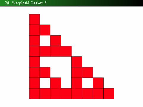
24. Sierpinski Gasket 3.

25. Sierpinski Gasket 4.
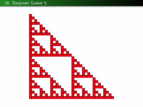
26. Sierpinski Gasket 5.

27. Sierpinski Gasket 6.

28. Sierpinski Gasket 7.

29. von Koch Snowflake
Figure: One of Three Sides of the Snowflake
Helge von Koch (1870–1924) was aSwedish mathematician who studiedsystems of infinitely many linear equations.He used pictures and geometric language inthe 1904 paper to construct his curve as anexample of a non-differentiable curve.Weierstrass’s 1872 description of such acurve used only formulas.
The von Koch Curve isobtained from IFSF = f1, f2, f3, f4 where incomplex notation z = x + iy ,
f1(z) =1
3z ,
f2(z) =eπi/3
3z +
1
3
f3(z) =e−πi/3
3z +
eπi/3 + 1
3
f4(z) =1
3z +
2
3.
Each contraction has λ = 13 .

30. von Koch Curve 1.

31. von Koch Curve 2.

32. von Koch Curve 3.

33. von Koch Curve 4.

34. von Koch Curve 5.

35. Barnsley’s Ferns
Images of Big Rectangle under F = f1, f2, f3.

36. Barnsley Fern F2
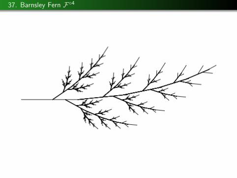
37. Barnsley Fern F4

38. Minkowski Curve
Figure: Minkowski Curve
The downward line in the middle consists oftwo segments of length 1
4 .
The Minkowski Curve isobtained from IFSF = f1, . . . , f8 where
f1(z) = 14z ,
f2(z) = i4z + 1
4
f3(z) = 14z + 1+i
4
f4(z) = − i4z + 2+i
4
f5(z) = − i4z + 1
2
f6(z) = 14z + 2−i
4
f7(z) = i4z + 3−i
4
f8(z) = i4z + 3
4
All λi = 14 .

39. Minkowski Curve 1.

40. Minkowski Curve 2.

41. Minkowski Curve 3.

42. Minkowski Curve 4.

43. Minkowski Curve 5.

44. Peano Curve
Figure: Peano Curve
This is called a space filling curve. Everypoint of the diamond is on the curve. Thereare many self-intersection points.
The Peano Curve is obtainedfrom IFS F = f1, . . . , f9where
f1(z) = 13z ,
f2(z) = i3z + 1
3
f3(z) = 13z + 1+i
3
f4(z) = − i3z + 2+i
3
f5(z) = −13z + 2
3
f6(z) = − i3z + 1
3
f7(z) = 13z + 1−i
3
f8(z) = i3z + 2−i
3
f9(z) = 13z + 2
3
The contractions all haveλi = 1
3 .

45. Peano Curve 1.

46. Peano Curve 2.

47. Peano Curve 3.

48. Peano Curve 4.

49. Peano Curve 5.
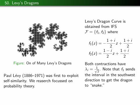
50. Levy’s Dragons
Figure: On of Many Levy’s Dragons
Paul Levy (1886–1971) was first to exploitself-similarity. We reaserch focussed onprobability theory.
Levy’s Dragon Curve isobtained from IFSF = f1, f2 where
f1(z) = −1 + i
2z +
1 + i
2
f2(z) =1− i
2z +
1 + i
2
Both contractions haveλi = 1√
2. Note that f1 sends
the interval in the southwestdirection to get the dragonto “snake.”

51. Levy’s Dragon 1.

52. Levy’s Dragon 2.
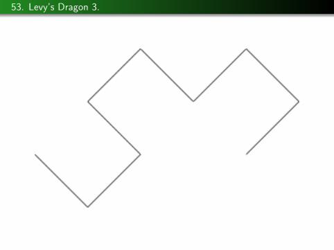
53. Levy’s Dragon 3.

54. Levy’s Dragon 4.

55. Levy’s Dragon 5.

56. Levy’s Dragon 6.
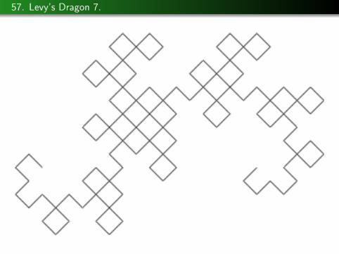
57. Levy’s Dragon 7.
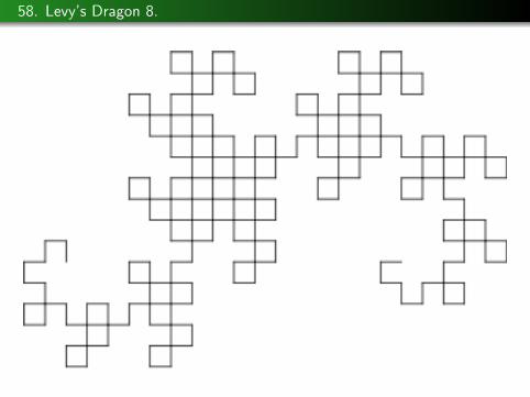
58. Levy’s Dragon 8.

59. Levy’s Dragon 9.
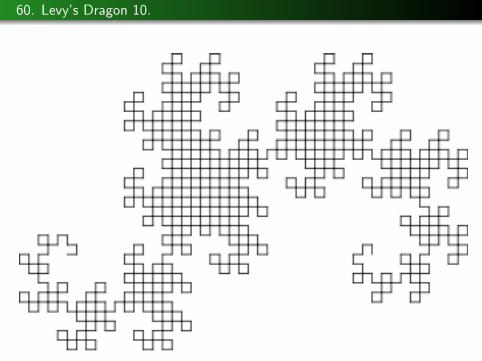
60. Levy’s Dragon 10.

61. Levy’s Dragon 11.

62. Levy’s Dragon 12.

63. Levy’s Dragon 13.

64. Levy’s Dragon 14.

65. Levy’s Dragon 15.

66. Self Similar Sets
A similarity transformation in Euclidean space is a linear map for x ∈ Rd
T (x) = λRx + b
where λ ≥ 0 is a scaling factor, R is a rotation matrix and b is atranslation vector. Reflections are also similarity transformations. In twodimensions, this is written in complex notation z = x + iy by
T (z) = az + b, (or T (z) = az + b)
where a = λe iθ ∈ C, λ = |a| is the norm and θ is the argument of a. Tis thus dilation by λ followed by rotation by angle θ and then bytranslation of b ∈ C.
A set A ⊂ Rd is self-similar if there is a similarity transformation T thatidentifies the a subset of S ⊂ A with itself T (S) = A.

67. Self-Similarity of the Snowflake Curve
Figure: The von Koch Curve isself-similar. e.g., the cyan subset issimilar to the whole curve.
The von Koch curve A is the fixedset of the IFS F = f1, f2, f3, f4,
A = F(A).
The cyan subset is S = f2(A), where
f1(z) = 13z ,
f2(z) = eπi3
3 z + 13
f3(z) = e−πi3
3 z + eπi3 +13
f4(z) = 13z + 2
3 .
are all invertible similaritytransformations. In particular
A = f −12 (S)
where the inverse is a similaritytransformation
z = f −12 (w) = 3e−πi3 w − e−
πi3
68. Hausdorff Measure of a Set
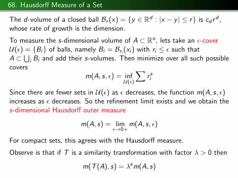
The d-volume of a closed ball Br (x) = y ∈ Rd : |x − y | ≤ r is cd rd ,whose rate of growth is the dimension.
To measure the s-dimensional volume of A ⊂ Rn, lets take an ε-coverU(ε) = Bi of balls, namely Bi = Bri (xi ) with ri ≤ ε such thatA ⊂
⋃i Bi and add their s-volumes. Then minimize over all such possible
coversm(A, s, ε) = inf
U(ε)
∑r si
Since there are fewer sets in U(ε) as ε decreases, the function m(A, s, ε)increases as ε decreases. So the refinement limit exists and we obtain thes-dimensional Hausdorff outer measure
m(A, s) = limε→0+
m(A, s, ε)
For compact sets, this agrees with the Hausdorff measure.
Observe is that if T is a similarity transformation with factor λ > 0 then
m(T (A), s) = λsm(A, s)

69. Facts About the s-Dimensional Hausdorff Outer Measure
Lemma
The set function A 7→ m(A, s) has the following properties
1 m(∅, s) = 0 for all s > 0 where ∅ is the empty set.
2 m(A1, s) ≤ m(A2, s) whenever A1 ⊂ A2.
3 (Subadditivity) For any finite or countable collection of subsets Ai ,
m
(⋃i
Ai , s
)≤∑i
m(Ai , s)
As a function of s, the function m(A, s) is infinite for small values of sand zero for large values, Only for one s can m(A, s) be something else.
Definition (Hausdorff Dimension)
dimH(A) = sups ∈ [0,∞) : m(A, s) =∞= infs ∈ [0,∞) : m(A, s) = 0

70. Hausdorff Dimension
Theorem
If s ≥ 0 is such that m(A, s) <∞ then m(A, t) = 0 for every t > s.
Proof.
m(A, t, ε) = infU(ε)
∑i
r ti = infU(ε)
∑i
r t−si r si
≤ infU(ε)
∑i
εt−sr si = εt−sm(A, s, ε).
Since t − s > 0 we have εt−s → 0 as ε→ 0+. But m(A, s, ε) ≤ m(A, s)because it is decreasing in ε, so
limε→0+
m(A, t, ε) = 0.
Corollary
If s ≥ 0 is such that m(A, s) > 0 then m(A, t) =∞ for every t < s.

71. Hausdorff Dimension of the Middle Thirds Cantor Set
We find the dimension by covering with balls.
The IFS for the Cantor set is F = f1, f2. If I = [0, 1] then the k-thapproximation to C is
Fk(I )
which consists of 2k intervals which are balls of radius 12·3k . If 1
2·3k ≤ εthis set of balls belongs to U(ε) and for s > 0,
m(C , ε) ≤∑
r si = 2k(
1
2 · 3k
)s
=1
2s
(2
3s
)k
This quantity tends to zero as ε→ 0 (same as k →∞) if 2 < 3s ors > ln 2
ln 3 . So dimH(C ) ≤ ln 2ln 3∼= .63.
Show dimH(C ) is larger than ln 2ln 3 is harder because we need to prove an
inequality that holds for ALL covers U(ε), but it is true.

72. Similarity Argument for Dimension of the Middle Thirds Cantor Set
We exploit the self-similarity to compute dimension of the Cantor Set.
Let’s assume s = dimH C and 0 < m(C , s) <∞. Because the IFS for theCantor set consists of similarity transformations F = f1, f2, withλi = 1
3 , the set is self-similar and C = f1(C ) ∪ f2(C ). By subadditivityand scaling for similarity transformations,
m(C , s) = m(f1(C ) ∪ f2(C ), s)
≤ m(f1(C ), s) + m(f2(C ), s)
= λsm(C , s) + λsm(C , s)
or
1 ≤ 2
(1
3
)s
.
Solving for s,0 = ln 1 ≤ ln 2− s ln 3
so
s ≤ ln 2
ln 3≈ .63.

73. Dimension for IFS of Similarity Transformations
If A is the attractor of an IFS F = f1, . . . , fk of similaritytransformations with 0 < λi < 1 and if the fi (A) are disjoint, then A isself similar. Assuming that s = dimH(A) and 0 < m(A, s) <∞
m(A, s) = m
(k⋃
i=1
fi (C )
)≤
k∑i=1
m(fi (C )) =k∑
i=1
λsi m(A, s)
which implies1 = λs1 + · · ·+ λsk = j(s)
Because the right side is a strictly decreasing function with j(0) = k > 1and lims→∞ j(s) = 0, there is a unique solution 1 = j(s), called thesimilarity dimension, which is an upper bound for dimH(A).
Because iterates may overlap, this may not be equal to dimH(S).Moran’s Theorem gives conditions so the similarity dimension equals theHausdorff dimension.
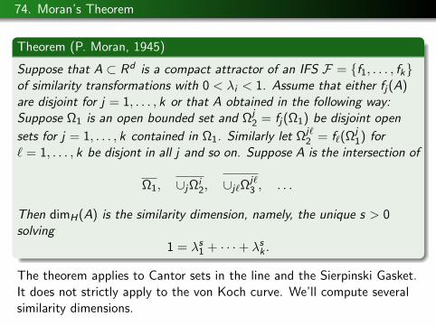
74. Moran’s Theorem
Theorem (P. Moran, 1945)
Suppose that A ⊂ Rd is a compact attractor of an IFS F = f1, . . . , fkof similarity transformations with 0 < λi < 1. Assume that either fj(A)are disjoint for j = 1, . . . , k or that A obtained in the following way:Suppose Ω1 is an open bounded set and Ωj
2 = fj(Ω1) be disjoint open
sets for j = 1, . . . , k contained in Ω1. Similarly let Ωj`2 = f`(Ωj
1) for` = 1, . . . , k be disjont in all j and so on. Suppose A is the intersection of
Ω1, ∪jΩi2, ∪j`Ωj`
3 , . . .
Then dimH(A) is the similarity dimension, namely, the unique s > 0solving
1 = λs1 + · · ·+ λsk .
The theorem applies to Cantor sets in the line and the Sierpinski Gasket.It does not strictly apply to the von Koch curve. We’ll compute severalsimilarity dimensions.

75. Hausdorff Dimension of the Sierpinski Gasket
Figure: Sierpinski Gasket
The Sierpinski Gasket isobtained from IFSF = f1, f2, f3 where
f1(z) = 12z ,
f2(z) = 12z + 1
2 ,
f3(z) = 12z + i
2 .
Each fi is a contraction withλ = 1
2 . Thus
1 = 3(12
)sor dimH(A) =
ln 3
ln 2∼= 1.58

76. Cantor Set with Unequal Intervals
Figure: Cantor Set with Unequal Intervals
This Cantor set is obtained from IFS on R
F = .4x , .5x + .5
of contractions with λ1 = .4 and λ2 = .5.
1 = (.4)s + (.5)s = j(s).
0.6 0.8 1.0 1.2 1.4
0.6
0.8
1.0
1.2
Plot of j(x)
x
0.4^
x +
0.5^
x
Using a root finder, thesolution is dimH(C ) = .867.
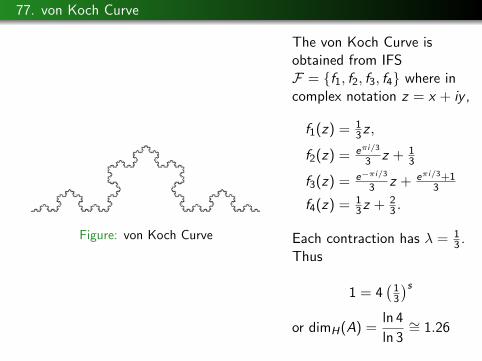
77. von Koch Curve
Figure: von Koch Curve
The von Koch Curve isobtained from IFSF = f1, f2, f3, f4 where incomplex notation z = x + iy ,
f1(z) = 13z ,
f2(z) = eπi/3
3 z + 13
f3(z) = e−πi/3
3 z + eπi/3+13
f4(z) = 13z + 2
3 .
Each contraction has λ = 13 .
Thus
1 = 4(13
)sor dimH(A) =
ln 4
ln 3∼= 1.26

78. Hausdorff Dimension of the Minkowski Curve
Figure: Minkowski Curve
f1(z) = 14z ,
f2(z) = i4z + 1
4
f3(z) = 14z + 1+i
4
The Minkowski Curve isobtained from IFSF = f1, . . . , f8 where
f4(z) = − i4z + 2+i
4
f5(z) = − i4z + 1
2
f6(z) = 14z + 2−i
4
f7(z) = i4z + 3−i
4
f8(z) = i4z + 3
4
All λi = 14 . Thus
1 = 8
(1
4
)s
or dimH(A) =ln 8
ln 4= 1.5.

79. Hausdorff Dimension of the Peano Curve
The Peano Curve is obtained from IFSF = f1, . . . , f9 where
f1(z) = 13z ,
f2(z) = i3z + 1
3
f3(z) = 13z + 1+i
3
f4(z) = − i3z + 2+i
3
f5(z) = −13z + 2
3
f6(z) = − i3z + 1
3
f7(z) = 13z + 1−i
3
f8(z) = i3z + 2−i
3
f9(z) = 13z + 2
3
The contractions all haveλi = 1
3 . Thus
1 = 9
(1
3
)s
or dimH(A) =ln 9
ln 3= 2.

80. Hausdorff Dimension of Levy’s Dragon
Figure: Levy Dragon
Levy’s Dragon Curve isobtained from IFSF = f1, f2 where
f1(z) = −1 + i
2z +
1 + i
2
f2(z) =1− i
2z +
1 + i
2
Both contractions haveλi = 1√
2. Thus
1 = 2
(1√2
)s
or dimH(A) =ln 2
ln√
2= 2.

81. Kiesswetter’s Nowhere Differentiable Function
Attractors of an IFS can be used to find relatively simple constructions ofmathematically interesting objects. In 1872, Weierstrass first wrote acontinuous nowhere differentiable function on I = [0, 1]
f (x) =∞∑i=1
bi cos(aiπx).
In 1916, Hardy sharpened conditions that it be continuous for 0 < b < 1and nowhere differentiable if also a > 1 and ab ≥ 1.
von Koch’ snowflake curve was contrived for the same purpose. But theeasiest construction is due to Kiesswetter in 1966.

82. Kiesswetter’s IFS
Figure: Yellow rectangle is mapped tofour rectangles by F
Kiesswetter considered the IFS
F = f1, f2, f3, f4
on [0, 1]× [−1, 1] where
f1(x) =
(14 00 −1
2
)(x1x2
),
f2(x) =
(14 00 1
2
)(x1x2
)+
(14−1
2
),
f3(x) =
(14 00 1
2
)(x1x2
)+
(140
)f4(x) =
(14 00 1
2
)(x1x2
)+
(3412
).
Each affine map shrinks horizontallyby 1
4 and vertically by 12 , thus has
contraction constants λi = 12 .

83. Kiesswetter’s Nondifferentiable Curve
By Hutchinson’s Theorem there is an attractor A for F . Kiesswettershowed that A is the graph of a curve A = (x , k(x)) : 0 ≤ x ≤ 1 whichis Holder Continuous
|f (x)− f (y)| ≤ C |x − y |12 for all x , y ∈ [0, 1]
and that it is nowhere differentiable.

84. Kieswetter’s Nondifferentiable Function 1.

85. Kieswetter’s Nondifferentiable Function 2.
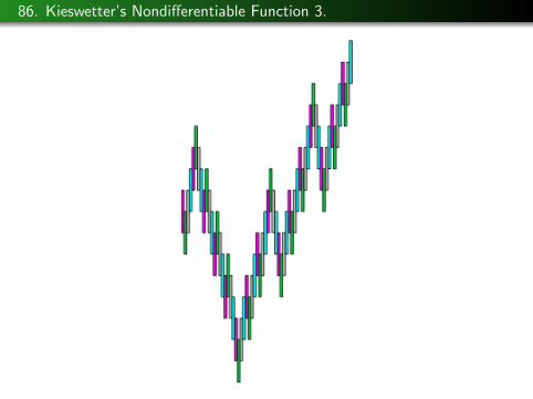
86. Kieswetter’s Nondifferentiable Function 3.

87. Kieswetter’s Nondifferentiable Function 4.
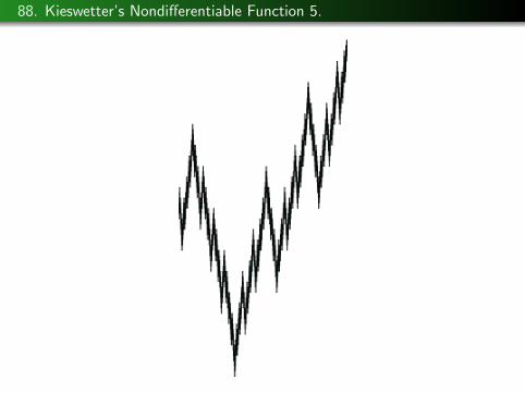
88. Kieswetter’s Nondifferentiable Function 5.

Thanks!