Embed Size (px)
Citation preview
FREQUENCY- AND PRESSURE- DEPENDENT
DYNAMIC SOIL PROPERTIES FOR SEISMIC
ANALYSIS OF DEEP SITESby
Dominic Assimaki
Diploma of Civil Engineering (1998)National Technical University of Athens.
Submitted to the Department of Civil and Environmental Engineering
in partial fulfillment of the requirements
for the degree of
MASTER OF SCIENCE IN CIVIL AND ENVIRONMENTAL ENGINEERING
at the
MASSACHUSETTS INSTITUTE OF TECHNOLOGY 19%MASSACHUSETTS INSTITUTE
OF TECHNOLOGY
February 2000
© Massachusetts Institute of Technology, 1999 FE R
IRARIES
Signature of Author............................................
DepartmenTofEilnd Environmental Engineering
7 November 3,1999
Certified by.................................
Eduardo Kausel, Professor of Civil and Environmetal Engineering
-77Thesis Supervisor
A ccepted by......................... .. . ........................................................................
Daniele Veneziano, Professor of Civil and Environmetal EngineeringChairman, Departmental Committee on Graduate Students

FREQUENCY- AND PRESSURE-DEPENDENT DYNAMIC SOIL
PROPERTIES FOR SEISMIC ANALYSIS OF DEEP SITES
by
Dominic Assimaki
Submitted to the Department of Civil and Environmental Engineeringon November 3, 1999 in partial fulfillment of the requirements for the degree of
Master of Science in Civil and Environmental Engineering.
ABSTRACT
Most of the analytical techniques for evaluating the response of soil deposits to strongearthquake motions employ numerical methods, initially developed for the solution of linearelastic, small - strain problems. Various attempts have been made to modify these methods to
handle nonlinear stress - strain behavior induced by moderate to strong earthquakes.
However, questions arise regarding the applicability of commonly used standardizedshear modulus degradation and damping curves versus shear strain amplitude. The most widelyemployed degradation and damping curves, are those originally proposed by Seed & Idriss, 1969.Laboratory experimental data (Laird & Stokoe, 1993) performed on sand samples, subjected tohigh confining pressures, show that for highly confined materials, both the shear modulus
reduction factor [G /GJ and the damping [ ] versus shear strain amplitude fall significantlyoutside the range used in standard practice, overestimating the capacity of soil to dissipateenergy.
The equivalent linear iterative algorithm also diverges when soil amplification isperformed in deep soft soil profiles, due to the assumption of a linear hysteretic damping beingindependent of frequency. High frequencies associated with small amplitude cycles of vibrationhave substantially less damping than the predominant frequencies of the layer, but are artificiallysuppressed when all frequency components of the excitation are assigned the same value ofhysteretic damping.
This thesis presents a simple four - parameter constitutive soil model, derived from
Pestana's (1994) generalized effective stress formulation, which is referred to as MIT-S1. Whenrepresenting the shear modulus reduction factors and damping coefficients for a granular soilsubjected to horizontal shear stresses imposed by vertically propagating shear [SH] waves, theresults are found to be in very good agreement with available laboratory experimental data.
Simulations for a series of " true" non-linear numerical analyses with inelastic (Masing-type) soils and layered profiles subjected to broadband earthquake motions, taking into accountthe effect of the confining pressure, are thereafter presented. The actual inelastic behavior isclosely simulated by means of equivalent linear analyses, in which the soil moduli and damping arefrequency dependent. Using a modified linear iterative analysis with frequency- and depth-dependent moduli and attenuation, a 1-km deep model for the Mississippi embayment nearMemphis, Tennessee, is successfully analyzed. The seismograms computed at the surface notonly satisfy causality (which cannot be taken for granted when using frequency-dependentparameters), but their spectra contain the full band of frequencies expected.
Thesis Supervisor: Eduardo KauselTitle: Professor of Civil and Environmental Engineering

4

5
ACKNOWLEDGEMENTS
This work would not have been accomplished, without the collaboration of many individuals.
I am first indebted to my thesis supervisor, Prof. Eduardo Kausel, who supported my work
and provided superior intellectual challenges. I have learned enormously from him and gained
insight to numerous problems that I have encountered throughout this challenging experience.
This work would not have been accomplished without his continuous support and
enthousiasm, without the energy that he dedicated, both as a mentor and as a friend.
I would also like to thank:
Prof. Andrew Whittle, for his contribution to the soil behavior and modelling aspects of this
thesis, for providing new ideas and insightful comments towards my work.
Prof. Kenneth Stokoe, for providing experimental data, essential for the completion of this
research project.
I would also like to acknowledge the partial economic support provided by Grant GT-2 from
the Mid-America Earthquake Center, under the sponsorship of the National Science
Foundation.
Acknowledgements also go out to:
Prof. George Gazetas, who encouraged me to pursue graduate studies in Civil Engineering. His
spirit and enthousiasm will always nourish my interest for research.
The faculty of the Mechanics and Materials group at MIT.
I am specially grateful to my fellow soiland dynamic friends from MIT: Federico Pinto, Jorge
Gonzales, Martin Nussbaumer, Yun Kim, Alexis Liakos, Christoph Haas, Attasit "Pong"
Korchaiyapruk, Dimitris Konstandakos, Karen Veroy, Joon Sang Park, Daniel Dreyer and
Monica Starnes, for the unforgettable experiences we have lived together, and for making my
life at MIT enjoyable and my effort less tiring.
To my family I owe the most. This work would not have been possible without their
continuous support and love. This thesis is dedicated to them, who have been the main source
of my strength throughout this challenging period of my life.
Finally, I would like to thank George Kokossalakis, who has been continuously there for me,
supporting my efforts, and helping me overpass obstacles that I wouldn't have managed to, if I
were on my own. This thesis is literary completed thanks to him.

6

7
To my family and George

8
9
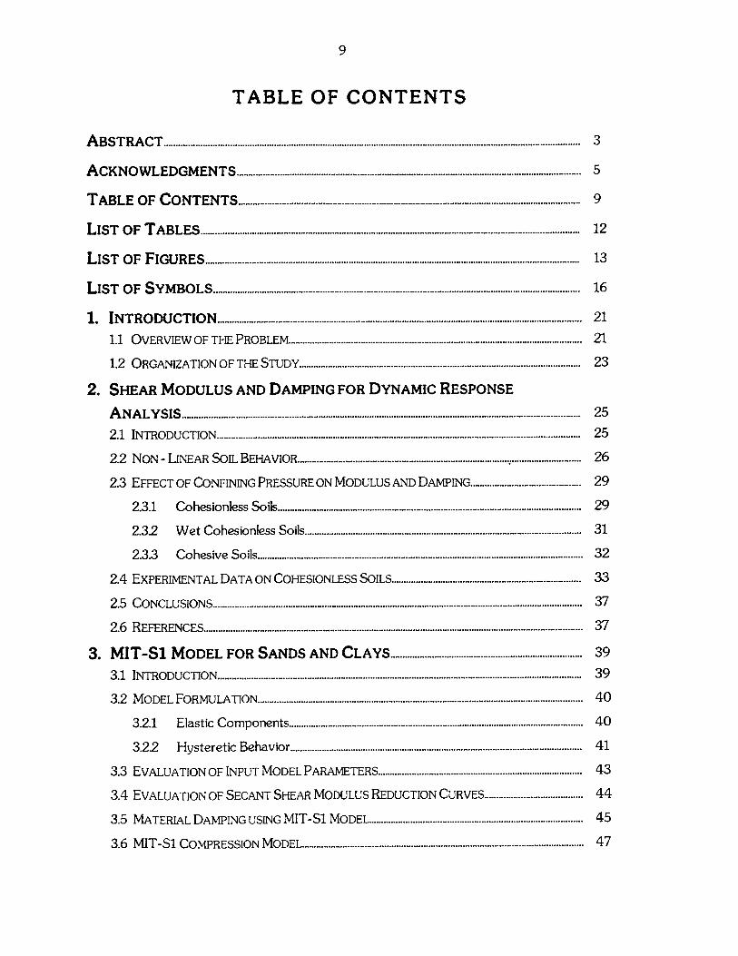
TABLE OF CONTENTS
A B S T R A C T .......................................................................................................................................................................... 3
A C K N O W L E D G M E N T S ............................................................................................................................................. 5
T A B L E O F C O N T E N T S ............................................................................................................................................ 9
L IS T O F T A B L E S ........................................................................................................................................................... 12
L IS T O F F IG U R E S ......................................................................................................................................................... 13
L IS T O F S Y M B O L S ...................................................................................................................................................... 16
1 . IN T R O D U C T IO N ..................................................................................................................................................... 2 1
1.1 O V ERV IEW O F T H E P RO BLEM ........................................................................................................................ 2 1
1.2 O RG A N IZA T IO N O F TH E S T U D Y ................................................................................................................... 2 3
2. SHEAR MODULUS AND DAMPING FOR DYNAMIC RESPONSE
A N A L Y S IS ................................................................................................................................................................... 2 5
2.1 IN T RO D U CT IO N ..................................................................................................................................................... 2 5
2.2 N O N - L IN EA R S O IL B EH A V IO R .................................................................................................................... 2 6
2.3 EFFECT OF CONFINING PRESSURE ON MODULUS AND DAMPING............................................ 29
2.3.1 C o hesio nless S o ils............................................................................................................................ 29
2.3 2 W et C o hesio nless S o ils................................................................................................................. 3 1
2.3.3 C o hesive S oils..................................................................................................................................... 3 2
2.4 EXPERIMENTAL DATA ON COHESIONLESS SOILS........................................................................... 33
2.5 C O N C LU SIO N S....................................................................................................................................................... 37
2.6 R EFEREN C ES........................................................................................................................................................... 37
3. M IT-Si M ODEL FOR SANDS AND CLAYS............................................................................. 39
3.1 IN TRO D U C T IO N ..................................................................................................................................................... 3 9
3.2 M O D EL FO R M U LA T IO N ..................................................................................................................................... 4 0
3.2.1 E lastic C o m p o nents........................................................................................................................ 4 0
3.2.2 H ysteretic B ehavio r....................................................................................................................... 4 1
3.3 EVALUATION OF INPUT MODEL PARAMETERS................................................................................. 43
3.4 EVALUATION OF SECANT SHEAR MODULUS REDUCTION CURVES....................................... 44
3.5 MATERIAL DAMPING USING M IT-Si MODEL....................................................................................... 45
3.6 M IT -S i C O M PR ESSIO N M O D EL...............................................................................................................--.. 4 7
10
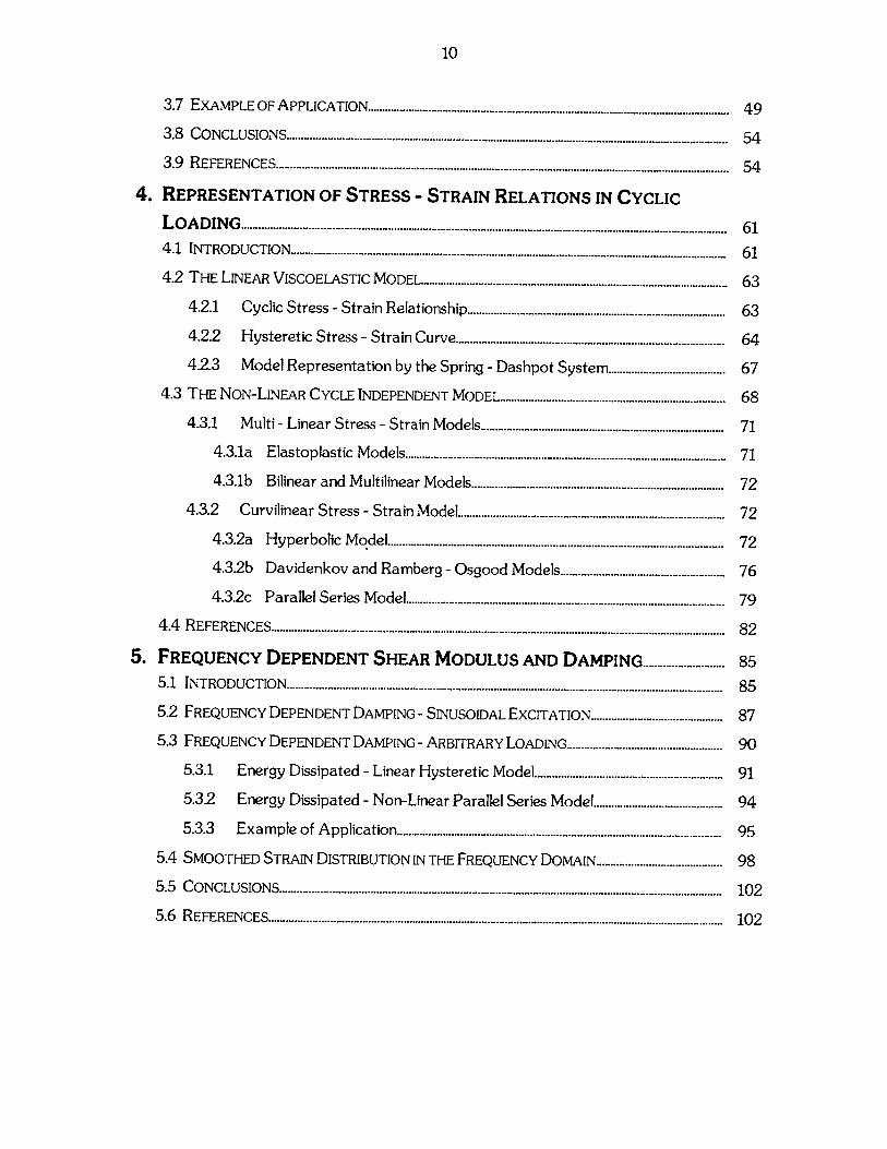
3.7 EXAMPLE OF APPLICATION........................................................................................................................... 49
3.8 CONCLUSIONS....................................................................................................................................................... 54
3.9 REFERENCES............................................................................. ................................................................ 54
4. REPRESENTATION OF STRESS - STRAIN RELATIONS IN CYCLICLOADING ............ ......................................................................................................... 614.1 INTRODUCTION............................................................................. ......................................................... 61
4.2 THE LINEAR VISCOELASTIC MODEL......................................................................................................... 63
4.2.1 Cyclic Stress - Strain Relationship ..................................................................................... 63
4.2.2 Hysteretic Stress - Strain Curve............................................................................................ 64
4.2.3 Model Representation by the Spring - Dashpot System....................................... 674.3 THE NON-LINEAR CYCLE INDEPENDENT MODEL............................................................................ 68
4.3.1 Multi - Linear Stress - Strain Models................................................................................. 71
4.3.1a Elastoplastic Models.............................................................................................................. 71
4.3.1b Bilinear and Multilinear Models..................................................................................... 724.3.2 Curvilinear Stress - Strain Model........................................................................................ 72
4.3.2a Hyperbolic Model................................................................................................................. 724.3.2b Davidenkov and Ramberg - Osgood Models .................. 76
4.3.2c Parallel Series Model............................................................................................................. 794.4 REFERENCES........................................................................................................................................................... 82
5. FREQUENCY DEPENDENT SHEAR MODULUS AND DAMPING.......................... 855.1 INTRODUCTION..................................................................................................................................................... 85
5.2 FREQUENCY DEPENDENT DAMPING - SINUSOIDAL EXCITATION............................................. 87
5.3 FREQUENCY DEPENDENT DAMPING - ARBITRARY LOADING..................................................... 90
5.3.1 Energy Dissipated - Linear Hysteretic Model........................................................... 91
5.3.2 Energy Dissipated - Non-Linear Parallel Series Model .............. 945.3.3 Exampe of.Applic tion...............................
5.3.3 Example of Applic ation ............................................................................................................... 95
5.4 SMOOTHED STRAIN DISTRIBUTION IN THE FREQUENCY DOMAIN.......................................... 98
5.5 CONCLUSIONS....................................................................................................................................................... 102
5.6 REFERENCES........................................................................................................................................................... 102
11
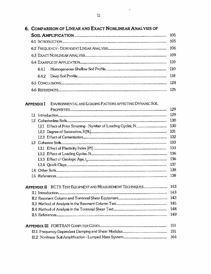
6. COMPARISON OF LINEAR AND EXACT NONLINEAR ANALYSIS OF
S O IL A M P L IF IC A T IO N ....................................................................................................................................6.1 IN TRO D UCTIO N .....................................................................................................................................................
6.2 FREQUENCY - DEPENDENT LINEAR ANALYSIS...................................................................................
6.3 E X A CT N O N LINEA R A N A LY SIS....................................................................................................................
6.4 E X A M PLE O F A PPLICA TIO N ............................................................................................................................
6.4.1 H om ogeneous S hallow Soil Profile......................................................................................
6.4.2 D eep S oil P rofile...............................................................................................................................
6.5 C O N CLU SIO N S.......................................................................................................................................................
6.6 R EFERENCES...........................................................................................................................................................
APPENDIX I ENVIRONMENTAL AND LOADING FACTORS AFFECTING DYNAMIC SOIL
PRO PERTIES ..........................................................................................................................................
1.1 Introductio n...........................................................................................................................................................
1.2 C ohesionless So ils..............................................................................................................................................
1.2.1 Ef fect of Prior Straining - Number of Loading Cycles, N............................................
1.2.2 D egree of S aturation, S [% ].............................................................................................. ..
1.2.3 E ffect of C em entation........................................................................................................................
1.3 C ohesive Soils......................................................................................................................................................
1.3.1 E ffect of P lasticity Index [P1]........................................................................................................
1.3.2 E ffect of L oading C ycles, N ............................................................................................................
I.3.3 Ef fect of Geologic Age, tg.........................................................................................
1.3.4 Q uick C lays...............................................................................................................................................
1.4 O ther Soils..............................................................................................................................................................
1.5 R eferences..............................................................................................................................................................
APPENDIX II RCTS TEST EQUIPMENT AND MEASUREMENT TECHNIQUES..................................
II.1 Introduction...........................................................................................................................................................
11.2 Resonant Column and Torsional Shear Equipment.....................................................................
11.3 M ethod of Analysis in the Resonant Column Test........................................................................
II.4 M ethod of Analysis in the Torsional Shear Test............................................................................
11.5 R eferences..............................................................................................................................................................
APPENDIX III FORTRAN COMPUTER CODES...............................................................................................
111.1 Frequency Dependent Damping and Shear Modulus...............................................................
111.2 Nonlinear Soil Amplification - Lumped Mass System..............................................................
105105
106
109
110
110
118
124
125
129129130130131132133133136136137138138
143
143143145148149
151151164
12
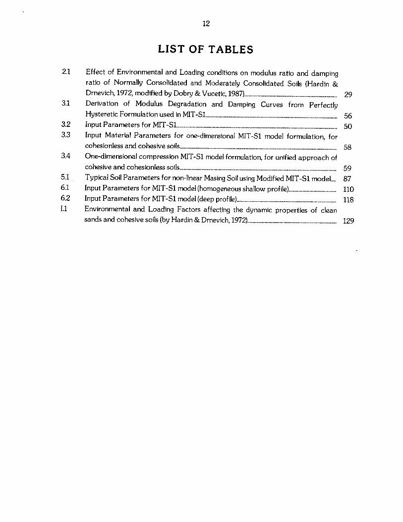
LIST OF TABLES
2.1 Effect of Environmental and Loading conditions on modulus ratio and dampingratio of Normally Consolidated and Moderately Consolidated Soils (Hardin &Drnevich, 1972, modified by Dobry & Vucetic, 1987)................................................................... 29
3.1 Derivation of Modulus Degradation and Damping Curves from PerfectlyHysteretic Form ulation used in M IT-Si.............................................................................................. 56
3.2 Input Param eters for M IT -Si......................................................................................................................... 503.3 Input Material Parameters for one-dimensional MIT-Si model formulation, for
cohesionless and cohesive soils......................................................................................................... 583.4 One-dimensional compression MIT-Si model formulation, for unified approach of
cohesive and cohesionless soils...................................................................................................................... 595.1 Typical Soil Parameters for non-linear Masing Soil using Modified MIT-Si model.... 876.1 Input Parameters for MIT-Si model (homogeneous shallow profile)................................... 1106.2 Input Parameters for MIT-Si model (deep profile).......................................................................... 1181.1 Environmental and Loading Factors affecting the dynamic properties of clean
sands and cohesive soils (by Hardin & Drnevich, 1972).................................................................. 129
13
LIST OF FIGURES
2.1 Loading - unloading at different strain amplitudes.......................................................................... 262.2 Secant modulus and damping ratio as function of maximum strain..................................... 27
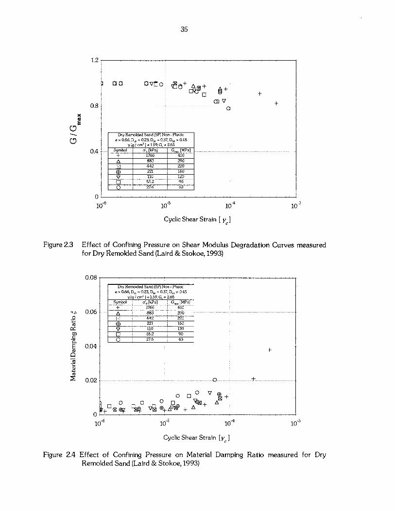
2.3 Effect of Confining Pressure on Shear Modulus Degradation Curves measured for
Dry Remolded Sand (Laird & Stokoe, 1993)....................................................................................... 35
2.4 Effect of Confining Pressure on Material Damping Ratio measured for Dry
Rem olded Sand (Laird & Stokoe, 1993).............................................................................................. 35
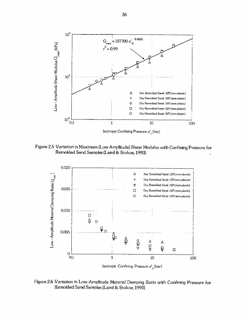
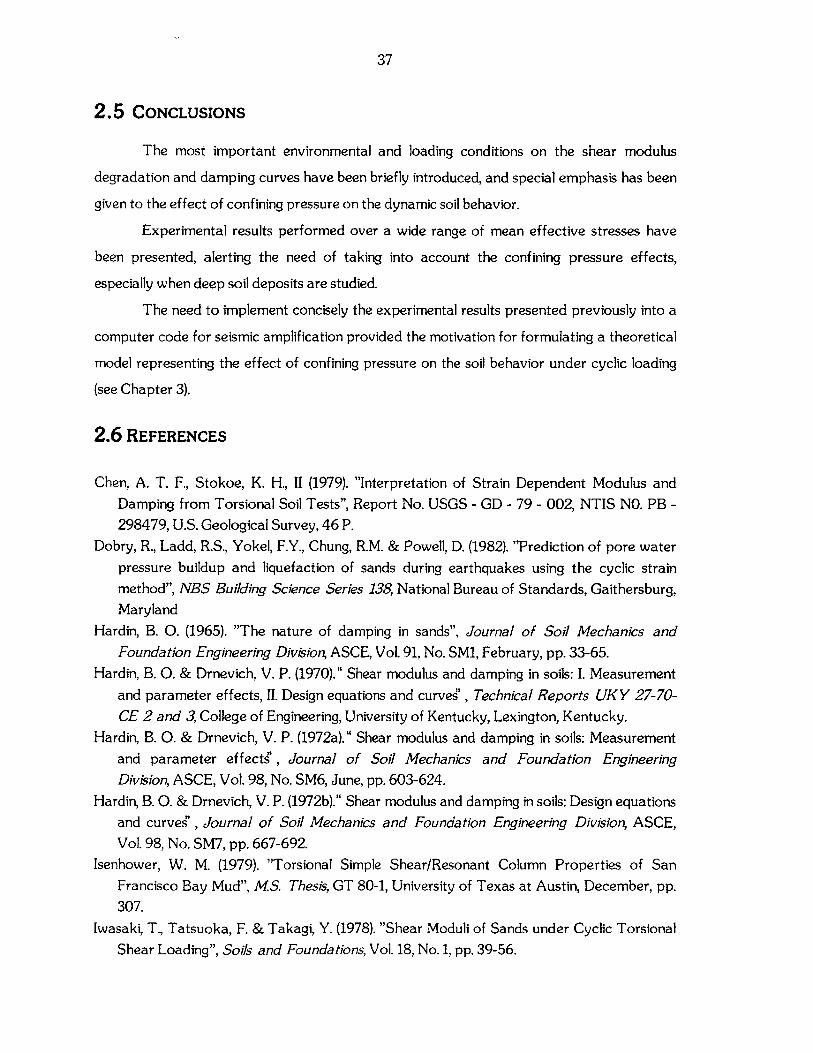
2.5 Variation in Maximum (Low Amplitude) Shear Modulus with Confining Pressure
for Remolded Sand Samples (Laird & Stokoe, 1993)................................................................... 36
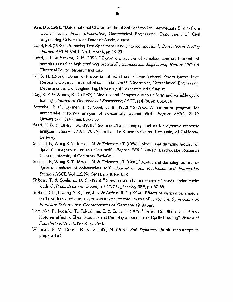
2.6 Variation in Low Amplitude Material Damping Ratio with Confining Pressure for
Remolded Sand Samples (Laird & Stokoe, 1993).......................................................................... 36
3.1 Comparison of Measured Degradation Curves for Remolded Sand Specimens
w ith proposed m odel predictions................................................................................................................. 45
3.2 Integration of Hysteresis loop to assess material damping........................................................ 46
3.3 Comparison of Experimental Material Damping on Dry Remolded Sand
Specimens and proposed model at different levels of confining pressure....................... 47
3.4 Void ratio as a function of mean effective stress............................................................................. 48
3.5 Soil profile used for 1-D soil amplification simulation (measured data from
Memphis area by Abrams & Shinozuka, 1997).................................................................:................. 50
3.6 Simulation of wave propagation in deep soil deposit for Kobe earthquake: (a)
Input Motion, (b) Surface Response, and (c) Fourier Spectra.................................................. 52
3.7 Simulation of wave propagation in deep soil deposit for Loma Prieta earthquake:
(a) Input Motion, (b) Surface Response, and (c) Fourier Spectra........................................... 53
4.1 Stress - strain hysteresis loop of a viscoelastic material............................................................... 66
4.2 T ypical V iscoelastic M odels............................................................................................................................ 67
4.3 Shear stress - strain relationship of: (a) An elastoplastic spring, and (b) A bilinear
sp ring .............................................................................................................................................................................. 7 2
4.4 Hyperbolic stress - strain relationship - Definition of reference strain................................ 73
4.5 Schematic illustration of the large strain limit value of material damping ratio............ 75
4.6 Schematic representation of an: (a) Elastoplastic Model, and (b) Elastoplastic
P arallel Series M odel............................................................................................................................................ 80
4.7 Multi-linear approximation of the backbone curve...................................................................... 80
5.1 Transfer functions at the surface of two soil deposits overlying rigid bedrock............ 87
5.2 Stiffness and Yield force of elastoplastic springs in parallel, using modified MIT-Si
m o d el.............................................................................................................................................................................. 8 8
5.3a Shear Strain time history and hysteresis loop of simulation using nonlinear model
of elastoplastic springs in parallel, with y / Y2= 2 ............................................................................. 89
5.3b Shear Strain time history and hysteresis loop of simulation using nonlinear model
of elastoplastic springs in parallel, with y1 / Y2= 4-----------------------------------------------------......................... 89
14
5.4 Inelastic Energy Dissipated in cyclic motion by a set of elastoplastic springs inparallel .......... ................................................................... .... ................................................... 90
5.5 Comparison of the Linear-Hysteretic Frequency-Dependent model with the Non-Linear Parallel Series model for the Kobe N-S earthquake (Vmax = 0.001)....................... 96
5.6 Comparison of the Linear-Hysteretic Frequency-Dependent model with the Non-Linear Parallel Series model for the Kobe N-S earthquake (Vma. = 0.05).......................... 97
5.7 (a) Scaled Fourier Transform of strain time history of various earthquakes, and (b)Smoothed Approximation of given data .................................................................................. 99
5.8 Frequency Dependent Damping and Shear Modulus Reduction Factor for theLinear Hysteretic Model, and comparison of the energy dissipated, evaluatedusing the exact, the smoothed strain FFT, and the parallel series model, for HelenaEarthquake scaled to Vmax = 0.001............................................................................................................... 100
5.9 Frequency Dependent Damping and Shear Modulus Reduction Factor for theLinear Hysteretic Model, and comparison of the energy dissipated, evaluatedusing the exact, the smoothed strain FFT, and the parallel series model, for HelenaEarthquake scaled to y . = 0.05............................................................................................................... 101
6.1 Frequency Dependent Damping and Shear Modulus for seismic wave propagation- Illustration of the M ethod......................................................................................................................... 1086.1a The Transfer function of the interface of interest is multiplied by the
smoothed strain Fourier Transform.................................................................................. 1076.1b The product of the smoothed strain Fourier Spectrum and the Transfer
Function is then scaled to the maximum value of the strain time history,and the frequency corresponding to the maximum value of the product isdefined.. ................................................................. ...... ........................................................ 108
6.1c The scaled Fourier Spectrum is assigned constant value of the strain timehistory maximum until the frequency corresponding the maximum of theproduct, is successively smoothed and used for the distribution of dampingand shear modulus reduction factors in the frequency domain.............................. 108
6.2 Idealization of the soil profile as a multi -degree of freedom system, for the exactnonlinear soil am plification analysis............................................................................................................ 109
6.3 Simulation of seismic analysis of a shallow homogeneous soil deposit for a puresinusoidal excitation [2.0 Hz], using frequency dependent and nonlinear analyses...... 112
6.4 Simulation of seismic analysis of a shallow homogeneous soil deposit for the
superposition of 2 sinusoidal excitations [2.0 and 8.0 Hz], using frequency
dependent and nonlinear analyses............................................................................................................... 1136.5a Simulation of seismic analysis of a shallow homogeneous soil deposit for the Kobe
Earthquake with maximum acceleration 0.01g, using frequency dependent andnonlinear analyses................................................. .... ......... _.................................................................... 114
15
6.5b Simulation of seismic analysis of a shallow homogeneous soil deposit for the KobeEarthquake with maximum acceleration 0.5g, using frequency dependent andnonlinear analyses................................................................................................................................................ 115
6.6a Simulation of seismic analysis of a shallow homogeneous soil deposit for thePasadena Earthquake with maximum acceleration 0.01g, using frequencydependent and nonlinear analyses.............................................................................................................. 116
6.6b Simulation of seismic analysis of a shallow homogeneous soil deposit for thePasadena Earthquake with maximum acceleration 0.5g, using frequencydependent and nonlinear analyses............................................................................................................... 117
6.7a Simulation of seismic analysis of a deep (1.0 km) soil deposit for the KobeEarthquake with maximum acceleration 0.01g, using frequency dependent andnonlinear analyses.................................................................................................................................................. 120
6.7b Simulation of seismic analysis of a deep (1.0 km) soil deposit for the KobeEarthquake with maximum acceleration 0.1g, using frequency dependent andnonlinear analyses.................................................................................................................................................. 121
6.7c Simulation of seismic analysis of a deep (1.0 km) soil deposit for the KobeEarthquake with maximum acceleration 0.5g, using frequency dependent andnonlinear analyses.................................................................................................................................................. 122
6.8a Comparison of the predicted duration of the surface response, for the Kobeearthquake scaled to maximum acceleration 0.01g......................................................................... 123
6.8b Comparison of the predicted duration of the surface response, for the LomaPrieta earthquake scaled to maximum acceleration 0.01g.......................................................... 124
1.1 Shear Modulus Reduction curve in the field, predicted assuming arithmetic andpercentage increase in m oduli........................................................................................................................ 137
II.1 Idealized Fixed - Free RCTS Equipment................................................................................................. 144
16
LIST OF SYMBOLS
CHAPTER 2
G Shear Modulus
Go, Gn. Small Strain Shear Modulus
Material Damping Ratio
Small Strain Material Damping Ratio
y Shear Strain Amplitude
,6E Area enclosed in the hysteresis loop
dm Effective mean principle stress
e Void Ratio
N Number of loading cycles
S[%] Degree of Saturation for cohesive soils
OCR Overconsolidation Ratio
c, cp Effective Strength Stress Parameters
T Shear Stress
rmax Maximum Shear Stress - Shear Strength
y, Reference Strain (= r. / Gm.)
U In-situ pore water pressure
PI Plasticity Index
KO Effective Coefficient of Lateral Earth Pressure at Rest
G, Specific Gravity
p Soil Density
D60 Soil Particle Diameter at which 60% of the soil is finer
D30 Soil Particle Diameter at which 30% of the soil is finer
Die Soil Particle Diameter at which 10% of the soil is finer
CHAPTER 3
o', Effective Overburden Pressure
Pa Atmospheric Pressure
K Tangent Bulk Modulus
Kmax Small strain bulk modulus
17
CQ Small Strain Stiffness at load reversal
P1 Poisson's Ratio at load reversal
o Non-linear Poisson's Ratio
re Stress Reversal Point
Z1 Non-dimensional distance in stress-space describing changes in the mean effective
stress and stress ratio relative to conditions at the stress reversal point
KONC Lateral Stiffness Coefficient of the Normally Consolidated Deposit
OCR1 Overconsolidation Ratio at Ko =1
p, Tangential Slope of the Hydrostatic Swelling Curve in a loge- loga space
CO, Small strain nonlinearity in shear
ce I CFriction angle at large strain (critical state) conditions
C, C, Q Parameters depending on mean effective stress level
PC Soil Matrix Compressibility - Slope of the Limiting Compression Curve (LCC) in a
loge - logo space
de Incremental Volume change
de e Elastic Incremental Volume change component
de P Plastic Incremental Volume change component
Cr Reference Stress at a unit void ratio
eo Formation Void Ratio (Void Ratio at dm=0)
dit Upper limit of effective stress, where compressibility of soil particles is significant
emi Lower limit of void ratio, where the void space becomes discontinuous and
assumptions of free drainage are no longer valid
V Shear Wave Velocity
cc Compression Index (= de l dlogu)
wL Liquid Limit
CHAPTER 4
co Angular Frequency or Circular Frequency
& Angle of phase difference
y, Shear Strain Amplitude
r. Shear Stress Amplitude
Y Shear Strain in complex variables
18
Shear Stress in complex variables
p Elastic Modulus
p Loss Modulus
p' Complex Modulus
n Loss Coefficient
W Energy Stored
A W Energy Dissipated
Tf Failure Stress - Shear Strength
4o Large Strain Material Damping Ratio
y Yield Strain
r, Yield Stress
a, r Parameters of the Ramberg - Osgood Model, defining the stress-strain relationship
k Spring Stiffness of the ith element, in the parallel series model
ry Critical Slipping Stress of the ith element, in the parallel series model
tan(a,) Tangent Stiffness at ( y, i)
N Number of elastoplastic springs
n Number of elements that remain elastic
CHAPTER 5
fi Fundamental Frequency of the soil column
Edl Energy dissipated by the ith element, in the parallel series model
u (x,t) Solution of the one-dimensional wave equation
c Wave propagation velocity
P(t) Instantaneous Power
P Average Power Dissipated
yRMs RMS value of the Shear Strain
APPENDIX I
N Number of loading cycles
yce Elastic Strain Threshold
Vc" Volumetric Strain Threshold
GN Shear Modulus after N cycles of loading
G1 Shear Modulus in the first cycle of loading

19
Degradation index
Geological Age of the soil deposit
Shear Modulus measured in the laboratory
Estimated value of Shear Modulus in the field
APPENDIX 11
I Mass Moment of Inertia of soil specimen
IM Mass Moment of Inertia of membrane
I0 Mass Moment of Inertia of rigid end mass at the top of the specimen
/ Length of the specimen
V Shear Wave Velocity of the specimen
Co,, Undamped Natural Circular Frequency of the system.
req Equivalent radius of the soil specimen
8 max Angle of twist at the top of the specimen
Z1, Z2 Two successive strain amplitudes of motion
6 Logarithmic Decrement
A Shear Strain Amplitude, defined as 0.707 Am for the half-power bandwidth
method
f, Frequency below the resonance where the strain amplitude is A
f2 Frequency above the resonance where the strain amplitude is A
f,. Resonant Frequency of the specimen
'c Particle velocity
T Period of motion
c Viscous Damping Coefficient
W, Energy Stored
Wd Energy Dissipated
cc Critical Damping Coefficient
m Mass of the system
6
t9
Gqa
Gfied

20
21
CHAPTER 1
INTRODUCTION
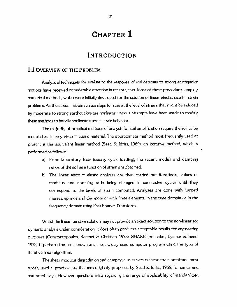
1.1 OVERVIEW OF THE PROBLEM
Analytical techniques for evaluating the response of soil deposits to strong earthquake
motions have received considerable attention in recent years. Most of these procedures employ
numerical methods, which were initially developed for the solution of linear elastic, small - strain
problems. As the stress - strain relationships for soils at the level of strains that might be induced
by moderate to strong earthquakes are nonlinear, various attempts have been made to modify
these methods to handle nonlinear stress- strain behavior.
The majority of practical methods of analysis for soil amplification require the soil to be
modeled as linearly visco - elastic material. The approximate method most frequently used at
present is the equivalent linear method (Seed & Idriss, 1969), an iterative method, which is
performed as follows:
a) From laboratory tests (usually cyclic loading), the secant moduli and damping
ratios of the soil as a function of strain are obtained.
b) The linear visco - elastic analyses are then carried out iteratively, values of
modulus and damping ratio being changed in successive cycles until they
correspond to the levels of strain computed. Analyses are done with lumped
masses, springs and dashpots or with finite elements, in the time domain or in the
frequency domain using Fast Fourier Transform.
Whilst the linear iterative solution may not provide an exact solution to the non-linear soil
dynamic analysis under consideration, it does often produces acceptable results for engineering
purposes (Constantopoulos, Roesset & Christian, 1973). SHAKE (Schnabel, Lysmer & Seed,
1972) is perhaps the best known and most widely used computer program using this type of
iterative linear algorithm.
The shear modulus degradation and damping curves versus shear strain amplitude most
widely used in practice, are the ones originally proposed by Seed & Idriss, 1969, for sands and
saturated clays. However, questions arise, regarding the range of applicability of standardized
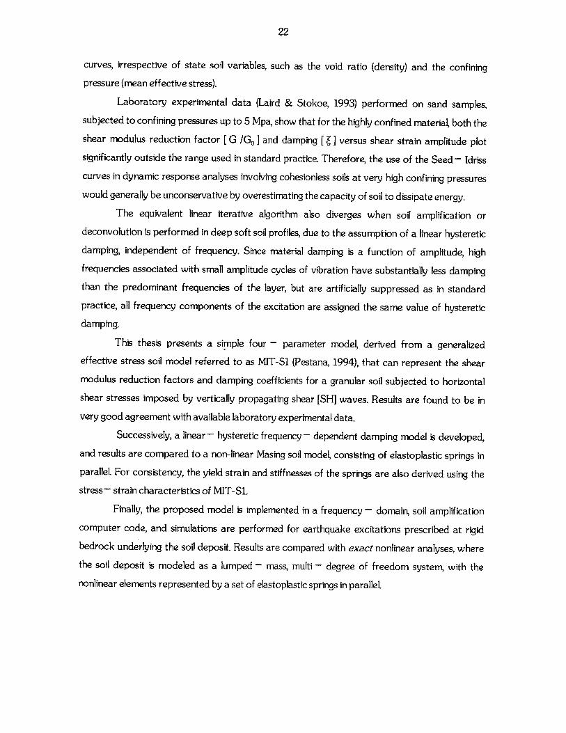
22
curves, irrespective of state soil variables, such as the void ratio (density) and the confining
pressure (mean effective stress).
Laboratory experimental data (Laird & Stokoe, 1993) performed on sand samples,subjected to confining pressures up to 5 Mpa, show that for the highly confined material, both the
shear modulus reduction factor [ G /Go ] and damping [ ] versus shear strain amplitude plot
significantly outside the range used in standard practice. Therefore, the use of the Seed - Idriss
curves in dynamic response analyses involving cohesionless soils at very high confining pressures
would generally be unconservative by overestimating the capacity of soil to dissipate energy.
The equivalent linear iterative algorithm also diverges when soil amplification or
deconvolution is performed in deep soft soil profiles, due to the assumption of a linear hysteretic
damping, independent of frequency. Since material damping is a function of amplitude, high
frequencies associated with small amplitude cycles of vibration have substantially less damping
than the predominant frequencies of the layer, but are artificially suppressed as in standard
practice, all frequency components of the excitation are assigned the same value of hysteretic
damping.
This thesis presents a simple four - parameter model, derived from a generalized
effective stress soil model referred to as MIT-S1 (Pestana, 1994), that can represent the shear
modulus reduction factors and damping coefficients for a granular soil subjected to horizontal
shear stresses imposed by vertically propagating shear [SH] waves. Results are found to be in
very good agreement with available laboratory experimental data.
Successively, a linear - hysteretic frequency - dependent damping model is developed,
and results are compared to a non-linear Masing soil model, consisting of elastoplastic springs in
parallel. For consistency, the yield strain and stiffnesses of the springs are also derived using the
stress- strain characteristics of MIT-Si.
Finally, the proposed model is implemented in a frequency - domain, soil amplification
computer code, and simulations are performed for earthquake excitations prescribed at rigid
bedrock underlying the soil deposit. Results are compared with exact nonlinear analyses, where
the soil deposit is modeled as a lumped - mass, multi - degree of freedom system, with the
nonlinear elements represented by a set of elastoplastic springs in parallel.
23
1.2 ORGANIZATION OF THE STUDY
Chapter 2 describes briefly the nonlinear characteristics of soil, when subjected to large
strain amplitudes, as well as the environmental and loading factors affecting the shear modulus
degradation and damping curves. The effect of confining pressure in successively described in
detail, for dry, wet cohesionless and cohesive soils. Finally, laboratory experimental data from
resonant column and torsional shear tests, performed on dry sand specimens under high confining
pressures, are presented, alerting the need of formulating a theoretical soil model, capable of
representing the effects of confining pressure on the nonlinear stress - strain soil characteristics.
Appendices to this chapter include:
i detailed description of the parameters affecting the stiffness and damping characteristics of
soils (Appendix I), and
ii. description of the resonant column and torsional shear equipment and measurement
techniques for the evaluation of secant modulus and damping ratio of the soil, as a function
of the shear strain amplitude (Appendix II).
Chapter 3 presents a simple four - parameter soil model, based on a generalized
effective stress model, referred to as MIT-Si (Pestana, 1994). The model parameters depend
both on the soil type as well as on soil state variables and characteristics, such as current void
ratio (density), confining pressure (mean effective stress) and small strain nonlinearity. Analytical
expressions for the shear modulus degradation and damping curves are derived, results are
compared with available experimental data and simulations are performed for soil amplification
of a deep soil deposit, successively compared to the results derived using Seed - Idriss standard
practice curves.
Chapter 4 describes in detail available linear viscoelastic and nonlinear stress - strain soil
models. For each model, general stress - strain equations are presented, as well as analytical
expressions for the equivalent hysteretic damping ratio.
Chapter 5 alerts initially one of the shortcomings of the equivalent - linear analysis, namely
the assumption of linear hysteretic damping, independent of frequency. The problem is stated by
simulations performed using a nonlinear model of elastoplastic springs in parallel, subjected to the
superposition of two sinusoidal motions. Successively, a linear - hysteretic frequency - dependent
model is presented, with stress - strain characteristics derived from MIT-S1. The performance of
the model under arbitrary loading conditions, namely an earthquake excitation, is compared to a
non-linear model, consisting of elastoplastic springs in parallel, the stiffness and yield deformation
24
of which, are also derived from the MIT-Sl formulation Appendices to this chapter include the
FORTRAN computer code used for the simulations (Appendix I.).
Chapter 6 presents soil amplification simulations, performed with the equivalent linear
iterative algorithm using frequency - and pressure - dependent dynamic soil properties. Results
are compared with these obtained by exact incremental nonlinear analyses, where the soil depositis simulated as a lumped mass multi - degree of freedom system, with the nonlinear elements
being represented by a parallel series model. For consistency of the comparison, the stress -strain characteristics of the nonlinear springs are derived from the one-dimensional formulation of
MIT-Si, described in Chapter 3. Appendices to this chapter include the FORTRAN computer
code used for the nonlinear soil amplification analysis (Appendix I1I2).
25
CHAPTER 2
SHEAR MODULUS AND DAMPING FOR DYNAMIC
RESPONSE ANALYSIS
2.1 INTRODUCTION
It is now standard practice in seismic engineering to take into consideration the non-linear
behavior of soils undergoing time-varying deformations caused by earthquakes. While it is in
principle possible to perform true incremental analyses in which the soil properties are adjusted
according to the load path and instantaneous levels of strain, this is seldom done in practice.
Instead, in the most widely used approach, approximate linear solutions are obtained using an
iterative scheme originally proposed by Seed and Idriss (1969). In this method, the soil properties
are chosen in each iteration in accordance with some characteristic measure of strain computed
in the previous iteration. While the linear iterative solution may not provide an exact solution to
the non-linear soil dynamics problem at hand, it does often produces acceptable results for
engineering purposes (Constantopoulos, Roesset & Christian, 1973). SHAKE (Schnabel, Lysmer
& Seed, 1972) is perhaps the best known and most widely used computer program using this type
of iterative linear algorithm.
Much progress has also been made recently in laboratory experiments attempting to
simulate the in-situ conditions that might exist in deep soil deposits (Laird & Stokoe, 1993). Soil
samples subjected in these tests to confining pressures as high as 5 Mpa have revealed
patterns of non-linear behavior that, while qualitatively similar to the response under lower
confining pressures, exhibited less degradation of shear modulus with strain (i.e. remained
nearly elastic). The damping due to hysteresis was correspondingly smaller. Testing at higher
confining pressures has proved a difficult task. Thus, it is desirable to develop an analytical
model that can supplement the experimental data, and can be used in computer models of
wave propagation in soils, such as SHAKE.
26
2.2 NON-LINEAR SOIL BEHAVIOR
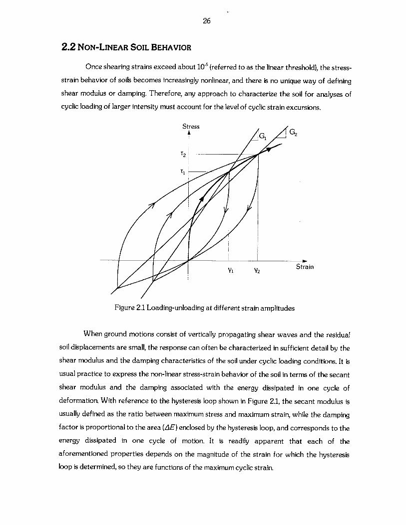
Once shearing strains exceed about 10-' (referred to as the linear threshold), the stress-
strain behavior of soils becomes increasingly nonlinear, and there is no unique way of defining
shear modulus or damping. Therefore, any approach to characterize the soil for analyses of
cyclic loading of larger intensity must account for the level of cyclic strain excursions.
Stress
Y1 V2 Strain
Figure 2.1 Loading-unloading at different strain amplitudes
When ground motions consist of vertically propagating shear waves and the residual
soil displacements are small, the response can often be characterized in sufficient detail by the
shear modulus and the damping characteristics of the soil under cyclic loading conditions. It is
usual practice to express the non-linear stress-strain behavior of the soil in terms of the secant
shear modulus and the damping associated with the energy dissipated in one cycle of
deformation. With reference to the hysteresis loop shown in Figure 2.1, the secant modulus is
usually defined as the ratio between maximum stress and maximum strain, while the damping
factor is proportional to the area (,6E) enclosed by the hysteresis loop, and corresponds to the
energy dissipated in one cycle of motion. It is readily apparent that each of the
aforementioned properties depends on the magnitude of the strain for which the hysteresis
loop is determined, so they are functions of the maximum cyclic strain.
27
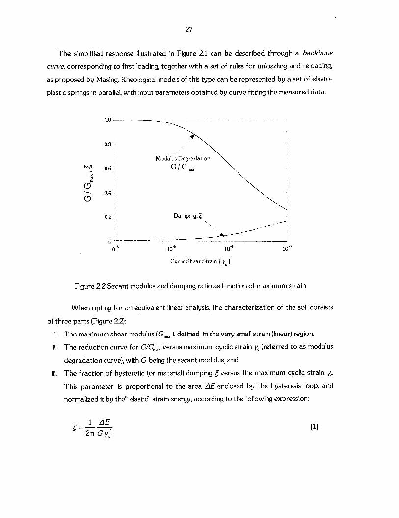
The simplified response illustrated in Figure 2.1 can be described through a backbone
curve, corresponding to first loading, together with a set of rules for unloading and reloading,
as proposed by Masing. Rheological models of this type can be represented by a set of elasto-
plastic springs in parallel, with input parameters obtained by curve fitting the measured data.
1.0
0.8
Modulus Degradation
0.6 G / G.
E
0.4
0.2 Damping, Z
010-6 105 10 10
Cyclic Shear Strain [ y
Figure 2.2 Secant modulus and damping ratio as function of maximum strain
When opting for an equivalent linear analysis, the characterization of the soil consists
of three parts (Figure 2.2):
i. The maximum shear modulus (Gax ), defined in the very small strain (linear) region.
ii. The reduction curve for G/Gm, versus maximum cyclic strain V (referred to as modulus
degradation curve), with G being the secant modulus, and
iii. The fraction of hysteretic (or material) damping ' versus the maximum cyclic strain ye.
This parameter is proportional to the area AE enclosed by the hysteresis loop, and
normalized it by the" elastid' strain energy, according to the following expression:
ri - {1}2ni G y
28
Typically G /Gm. decreases and [ increases as ye becomes larger, and in fact it has
been noticed that a fast decrease in GIG, with ye , corresponding to a strongly nonlinear soil,
is associated with a strong increase of [' with y, in the same soil, and vice versa.
In the case of dry cohesionless soils, the physical origin of the variation in modulus and
damping with cyclic strain, as reflected in the shapes of the curves in Figure 2.2, is now well
understood. Both parameters are related to the frictional behavior at the interparticle
contacts and the rearrangement of the grains during cyclic loading (Dobry et al., 1982; Ng and
Dobry, 1992; Ng and Dobry, 1994). Therefore, even crude analytical models of particles can
be used to mimic the shear modulus reduction factor, G / Gmax, and material damping, E
versus yc curves, provided that they include friction and allow for particle rearrangements.
It should be noted however that reversible behavior is associated with minimal
rearrangement of particle contacts and irrecoverable, plastic, strains become significant only
at strain levels ye > 107. For smaller cyclic strain amplitudes therefore, dissipation of energy
must be related to frictional behavior at contacts, yet the physical mechanisms related to
nonlinear stress - strain phenomena below the volumetric threshold (y "- 107) are not clearly
defined.
A comprehensive survey of the factors affecting the shear moduli and damping
factors of soils and expressions for determining these properties have been presented by
Hardin & Drnevich (1972a & b). In this study it was suggested that the primary factors
affecting moduli and damping factors are:
* Strain amplitude, y
* Effective mean principle stress, 'm* Void ratio, e
* Number of cycles of loading, N
* Degree of saturation for cohesive soils, S[%]
and that less important factors include:
* Octahedral shear stress
" Overconsolidation ratio, OCR
" Effective strength stress parameters, c and cp'
" Time effects
29
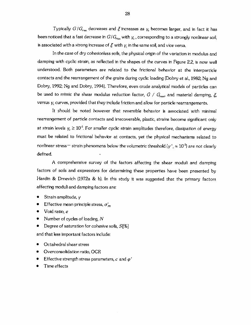
Table 2.1 summarizes the effect of these parameters on the shear modulus
degradation curves and damping. Further details can be found in Appendix I of the present
study.
Increasing Factor G / Gmax
Cyclic Strain, yc Decreases with yc Increases with yc
Confining Pressure, a'm Increases with o'm Decreases with o'm(effect decreases with increasing PI) (effect decreases with increasing PI)
Void Ratio, e Increases with e Decreases with e
Geologic Age, tg May increase with tg May decrease with tg
Cementation, c May increase with c May decrease with c
Overconsolidation Ratio, OCR Not affected Not affected
Plasticity Index, PI Increases with PI Decreases with PI
Strain Rate, dy/dt G / Gmax probably not affected if Stays constant or may increase
G and Gmax measured at the with dy/dt
same strain rate d y/dt
Number of Loading Cycles, N Decreases after N cycles of large yc Not significant for moderate
for clays; for sands can increase (drained yc and number of cycles, N
conditions) or decrease (undrained conditions)
Table 2.1 Effect of Environmental and Loading conditions on modulus ratio and damping ratioof Normally Consolidated and Moderately Consolidated Soils (Hardin & Drnevich,1972, modified by Dobry & Vucetic, 1987)
Amongst the aforementioned parameters affecting the dynamic response of soils,
apart from the well known strain amplitude (y), the effective mean principle stress (o'i) is more
pronounced in the dynamic analysis of deep soil deposits studied herein, and it will be
therefore analyzed separately in the proceeding section.
2.3 EFFECT OF CONFINING PRESSURE ON MODULUS AND
DAMPING
2.3.1 COHESIONLESS SOILS
The modulus degradation and damping curves most often used for dry cohesionless
soils, such as sands, gravels and cohesionless silts, are those proposed by Seed and Idriss
(1970). Based on experimental data by Hardin & Drnevich (1970) and others, these standard
curves are extensively used in equivalent linear analysis of earthquake excitations and machine
vibrations. The Seed & Idriss approach assumes that the G / Gmax and j'curves are essentially
the same for sands, gravels and cohesionless silts. Their generic response curves, assume that
30
the degradation curves are independent of the cycle number considered, as well as the void
ratio (or relative density), sand type and confining pressure, factors which, according to the
same study, do affect significantly the maximum shear modulus G,,,, defined below the
elastic threshold, ye 10-'.
Laboratory measurements provide evidence in support of some of these simplifying
assumptions. They show that void ratio, overconsolidation, sand type and cycle number
(Dobry et al., 1982, Iwasaki et al., 1978) do indeed have relatively small influence on the
measured backbone curves. They also show that the method of sand deposition, existence of
static shear stress, grain size (sands vs. gravels) are also of secondary importance (Hardin,1965, Hardin & Drnevich, 1972a, Tatsuoka et al., 1979, Seed et al., 1986). However, the
influence of the confining pressure is significant and cannot possibly be ignored, especially
when performing dynamic analyses for deep soil sites.
A number of laboratory studies (see Section 2.4) on hydrostatically' consolidated
sands have shown that their stress-strain response becomes more linear as the confining
pressure increases (i.e. for a given shear strain amplitude, y, as o increases, G / Gnax increases
and decreases). In addition, large confining pressures lead to substantial reductions in
material damping at small strain, i.e. [i. The reason for these effects with increasing o is
related to the different rates at which the small strain modulus and the shear strength of the
soil increase when the pressure increases (Hardin & Drnevich, 1972a, Seed et al., 1986, Laird &
Stokoe, 1993).
To illustrate this assertion, consider the hyperbolic model frequently used to represent
the stress strain behavior of soils. In this model, the backbone curve is defined in terms of two
parameters, namely the small stain shear modulus Gmax and the shear strength rmax. The
hyperbolic equation for the backbone curve is:
r = {2}(1/ Gma+ y /r)ax
Alternatively, T = [ y / ( y, + )] Tmax, in which y = Tmax / Gma. is a reference strain (Hardin &
Drnevich, 1972b). Therefore, the corresponding modulus degradation curve is only a function
of the reference strain, namely:
'Laboratory data show minor influence of KO on the shear modulus degradation and damping curves (Hardin &Drnevich, 1972a)
31
G 1G + ( I 1{ 3 }
Gax 1+(y / y,
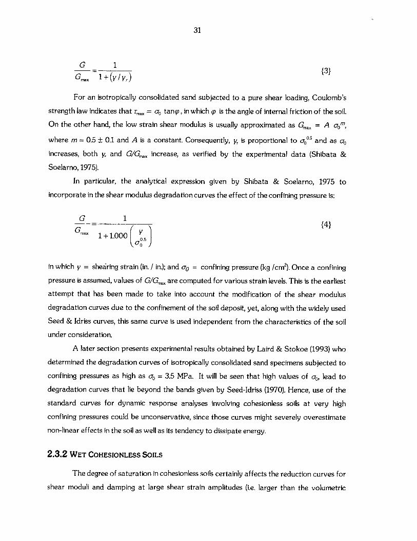
For an isotropically consolidated sand subjected to a pure shear loading, Coulomb's
strength law indicates that rm = co tancp, in which qp is the angle of internal friction of the soil.
On the other hand, the low strain shear modulus is usually approximated as Gma. = A com,
where m = 0.5 ± 0.1 and A is a constant. Consequently, y is proportional to ac and as ao
increases, both y, and GIG. increase, as verified by the experimental data (Shibata &
Soelarno, 1975).
In particular, the analytical expression given by Shibata & Soelarno, 1975 to
incorporate in the shear modulus degradation curves the effect of the confining pressure is:
G 1
a 1±1.000
in which y = shedring strain (in. / in.); and ao = confining pressure (kg /cm 2). Once a confining
pressure is assumed, values of G/Gma. are computed for various strain levels. This is the earliest
attempt that has been made to take into account the modification of the shear modulus
degradation curves due to the confinement of the soil deposit, yet, along with the widely used
Seed & Idriss curves, this same curve is used independent from the characteristics of the soil
under consideration.
A later section presents experimental results obtained by Laird & Stokoe (1993) who
determined the degradation curves of isotropically consolidated sand specimens subjected to
confining pressures as high as co = 3.5 MPa. It will be seen that high values of o, lead to
degradation curves that lie beyond the bands given by Seed-Idriss (1970). Hence, use of the
standard curves for dynamic response analyses involving cohesionless soils at very high
confining pressures could be unconservative, since those curves might severely overestimate
non-linear effects in the soil as well as its tendency to dissipate energy.
2.3.2 WET COHESIONLESS SOILS
The degree of saturation in cohesionless soils certainly affects the reduction curves for
shear moduli and damping at large shear strain amplitudes (i.e. larger than the volumetric
32
threshold ye > 10-3). For smaller strain amplitudes, the soil behavior can be approximated as
uncoupled, i.e. minimum volume change and pore pressure generation, are introduced by
shearing. Therefore, it is presumed that the curves for dry materials may also be applicable to
saturated granular soils for shear strain amplitudes yc: 1073 , with the response controlled by
the in-situ effective confining pressure:
a=a-u {5}
where: u the in-situ pore water pressure.
Clearly, if water is not trapped between the soil particles during shear, it does not
participate in the stress-strain response or in the energy dissipation in the material. In such
case, damping is completely caused by friction due to interactions between the particles, as if
the soil was dry. It should be noted, however, that this might not apply to small strain, high
frequency cyclic loads in a resonant column test. In such case, damping values will be higher for
a saturated material because of viscous effects caused by the relative movement between the
solid phase and the pore water. This difference in damping between dry and saturated soil is
generally not significant for low-frequency dynamic phenomena such as earthquakes, but may
be relevant to high-frequency vibrations such as generated by explosions and machine
vibrations.
2.3.3 COHESIVE SOILS
Based on experimental data on normally consolidated undisturbed specimens of clay
and silt obtained from several depths at a site in Japan, tested under confining pressures
ranging from 0.2 to 0.7 kg/cm 2, two general features can be clearly observed:
i. For the only specimen of non-plastic silt (PI = 0), the shear modulus degradation curve
plots together with the sand curve, and
ii. The shear modulus degradation curves of the rest of the cohesive soil samples plot
above the sand curve, with their location being higher when the PI is higher, more or less
irrespective of confining pressure.
These results are typical of many others published in the literature, indicating that the
shear modulus degradation (G / Gma.) and damping (f) curves of saturated cohesive soils in
sedimentary deposits are essentially independent of effective confining pressure, void ratio,
33
and overconsolidation and are largely a function of the Plasticity Index (PI) of the clay (Zen, et
al., 1978; Kokusho, et al., 1982; Ishihara, 1986; Romo & Jaime, 1986; Dobry & Vucetic, 1987;
Sun, et al.,1988; Dobry & Vucetic, 1991).
While comparisons between G /Gm. and curves of natural clays do show an
influence of void ratio, e, it is primarily due to the fact that high plasticity clays tend to have
greater values of e than low plasticity soils, with the effect of e largely disappearing when the
Plasticity Index of the clay is considered (Lodde & Stokoe, 1982; Vucetic & Dobry, 1991).
2.4 EXPERIMENTAL DATA ON COHESIONLESS SOILS
To determine the dynamic properties of granular soils at significant depths, laboratory
tests were performed by Laird & Stokoe (1993), at UT Austin. The objective of the
experiments was to determine the dynamic properties of soils at significant depths, both for
dry and saturated specimens at confining pressures up to o = 3.5 MPa. The results of these
tests demonstrate the effects of confining pressure on shear modulus and damping described
previously.
Washed mortar sand was used to build remolded sand specimens. The sand is poorly-
graded, with a medium to fine grain size, and classifies as (SP) in the Unified Classification
System. For the construction of the remolded sand specimens, the undercompaction method
(Ladd, 1978) was used.
Resonant column and torsional shear (RCTS) equipment was used to investigate the
dynamic characteristics of the samples tested at high confining pressures, developed by the
group at UT Austin (Isenhower, 1979, Lodde, 1982, Ni, 1987, and Kim, 1991). The equipment is
of the fixed-free type, with the bottom of the specimen fixed and the torsional excitation
applied at the top. Both resonant column (RC) and torsional shear (TS) tests were performed
in a sequential series on the same specimen over a range of shearing strains from about 10-6 to
slightly more than 10-3, by changing the frequency of the forcing function.
The primary difference between the two types of tests is the excitation frequency. In
the RC test, frequencies above 20 Hz are required and inertia of the specimen and drive
system are needed to analyze these measurements. On the other hand, slow cyclic loading with
frequencies generally below 5 Hz is prescribed in the TS tests and inertia does not enter the
data analysis. Further information about the test equipment and measurement techniques
34
used for the aforementioned laboratory program, can be found in Appendix II of the present
study.
In addition to the remolded specimens, four undisturbed specimens, two from
Treasure Island and two from Lotung were tested at high confining pressures. The samples
from Treasure Island were obtained from depths of 33 ft (10.1 m) and 110 ft (33.6 m) and were
classified as a sand with silt (described as SP-SM in the Unified Classification System). The
Lotung samples include a silty sand (SM) from a depth of 59 ft (18.0 m) and a silt (ML) from a
depth of 146ft (44.5 m). For the undistirbed specimens, the confining pressures tested were
based on the estimated in situ mean efffective stress, assuming the effective coefficient of
earth pressure at rest KO = 0.5. The behavior of the undisturbed samples, tested over a range
of confining pressures varying from 0.25 om + 4.00 or , was very similar to that of the
remolded specimens.
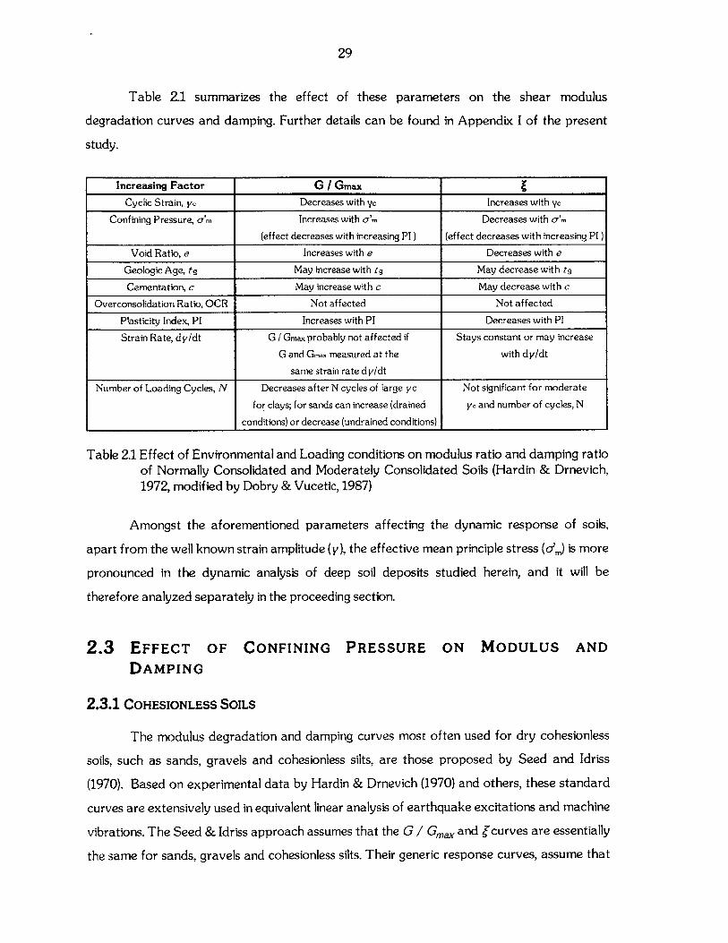
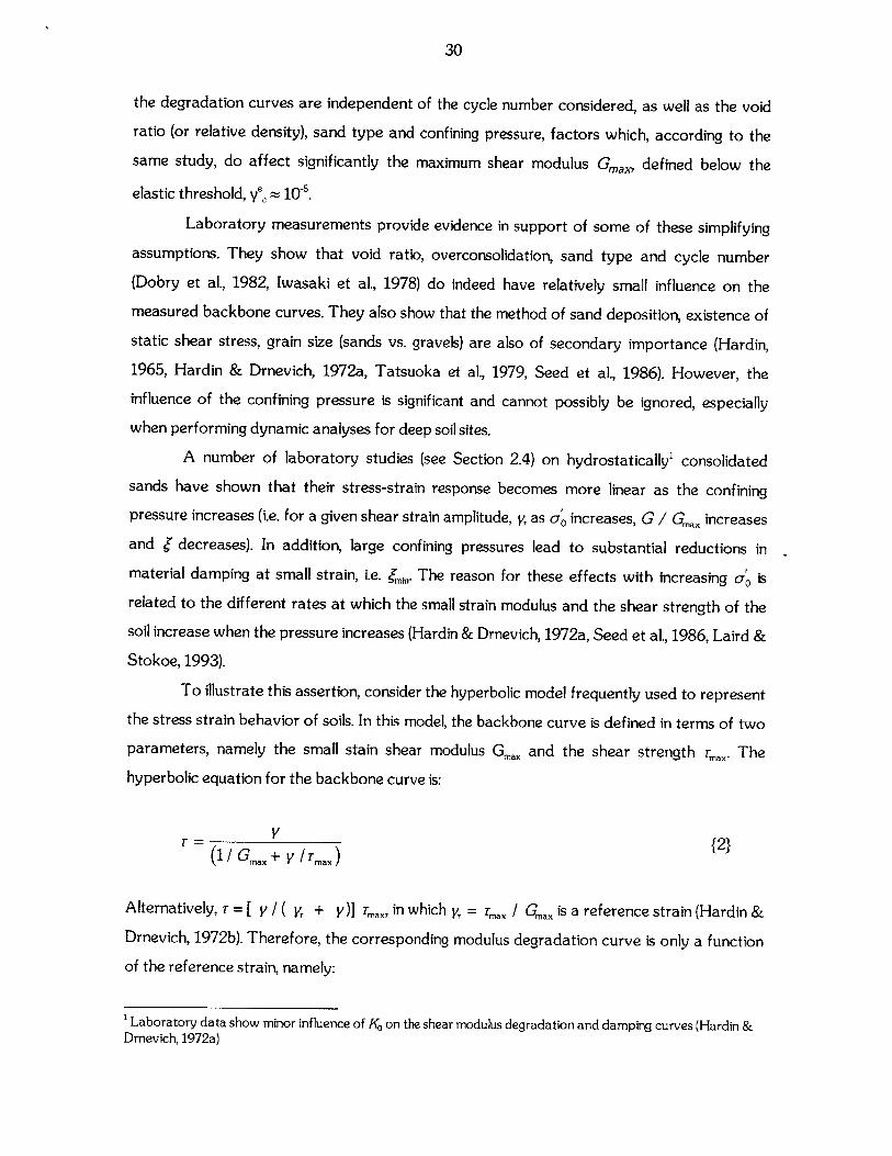
Figures 2.3 and 2.4 show the shear modulus degradation and material damping curves
of a remolded sand specimen for different values of confining pressure respectively. The
results show that the elastic threshold (i.e. the cyclic strain at the linear limit), increases with the
confining pressure.
Figures 2.5 and 2.6, on the other hand, show the dependence with the level of
confinement of the small-strain shear modulus, G, and material damping, [.. Clearly,
materials with higher confinement are stiffer at small values of strains.
10-5
35
1.2
0.8
E
0.4.
010-6 10 3
Cyclic Shear Strain [ y]
Figure 2.3 Effect of Confining Pressure on Shear Modulus Degradation Curves measuredfor Dry Remolded Sand (Laird & Stokoe, 1993)
0.08
0.06 1-0)
E
Q)
0.041F
0.02 1
0 L-!10-6
0
10~5
-- --± -- - - - -
--------
Cyclic Shear Strain [V ]
Figure 2.4 Effect of Confining Pressure on Material Damping Ratio measured for DryRemolded Sand (Laird & Stokoe, 1993)
00CI OVO O+ A +E~ ~ +
cliv +
Dry Remolded Sand (SP) Non - Plastice = 0.66, D,, = 0.23, D3 = 0.37, Ds, = 0.45
y [g /cm' ]=1.59, G, =2.65Symbol - do [kPa] G [MPa]
+ 1766 410883 290
p 442 220221 160110 120
0 55.2 90o 27.6 63
Dry Remolded Sand (SP) Non - Plastice = 0.66, D, = 0.23, D, = 0.37, D, = 0.45
y [g / cm3 I = 1.59, G, = 2.65Symbol 00 [kPa] G.. [MPa]
+ 1766 410A 883 29071 442 220
221 160V 110 1200 55.2 90o 27.6 63
+0-
o +D
36
106
E
C,,
~0
E
0
104 L0.1 1 10 100
Isotropic Confining Pressure do [bar]
Figure 2.5 Variation in Maximum (Low Amplitude) Shear Modulus with Confining Pressure forRemolded Sand Samples (Laird & Stokoe, 1993)
0.020
0
E
E
0
0.015
0.010
0.0051
0.0. 1 10 100
Isotropic Confining Pressure d7 [bar]
1
Figure 2.6 Variation in Low-Amplitude Material Damping Ratio with Confining Pressure forRemolded Sand Samples (Laird & Stokoe, 1993)
A Sat. Remolded Sand (SP) (non-plastic)
+ Dry Remolded Sand (SP) (non-plastic)
v Dry Remolded Sand (SP) (non-plastic)----------- o Dry Remolded Sand (SP) (non-plastic)
o Dry Remolded Sand (SP) (non-plastic)
V 0
---------------- --- --------- ----- ------ --A- ---
~D A A A
10 5
37
2.5 CONCLUSIONS
The most important environmental and loading conditions on the shear modulus
degradation and damping curves have been briefly introduced, and special emphasis has been
given to the effect of confining pressure on the dynamic soil behavior.
Experimental results performed over a wide range of mean effective stresses have
been presented, alerting the need of taking into account the confining pressure effects,
especially when deep soil deposits are studied.
The need to implement concisely the experimental results presented previously into a
computer code for seismic amplification provided the motivation for formulating a theoretical
model representing the effect of confining pressure on the soil behavior under cyclic loading
(see Chapter 3).
2.6 REFERENCES
Chen, A. T. F., Stokoe, K. H., 11 (1979). "Interpretation of Strain Dependent Modulus andDamping from Torsional Soil Tests", Report No. USGS - GD - 79 - 002, NTIS NO. PB -298479, U.S. Geological Survey, 46 P.
Dobry, R., Ladd, R.S., Yokel, F.Y., Chung, R.M. & Powell, D. (1982). "Prediction of pore waterpressure buildup and liquefaction of sands during earthquakes using the cyclic strainmethod", NBS Building Science Series 138, National Bureau of Standards, Gaithersburg,Maryland
Hardin, B. 0. (1965). "The nature of damping in sands", Journal of Soil Mechanics andFoundation Engineering Division, ASCE, Vol. 91, No. SM1, February, pp. 33-65.
Hardin, B. 0. & Drnevich, V. P. (1970)." Shear modulus and damping in soils: I. Measurementand parameter effects, II. Design equations and curved , Technical Reports UKY 27-70-CE 2 and 3, College of Engineering, University of Kentucky, Lexington, Kentucky.
Hardin, B. 0. & Drnevich, V. P. (1972a)." Shear modulus and damping in soils: Measurementand parameter effects, Journal of Soil Mechanics and Foundation Engineering
Division, ASCE, Vol. 98, No. SM6, June, pp. 603-624.Hardin, B. 0. & Drnevich, V. P. (1972b)." Shear modulus and damping in soils: Design equations
and curveg', Journal of Soil Mechanics and Foundation Engineering Division, ASCE,Vol. 98, No. SM7, pp. 667-692.
Isenhower, W. M. (1979). "Torsional Simple Shear/Resonant Column Properties of SanFrancisco Bay Mud", MS. Thesis, GT 80-1, University of Texas at Austin, December, pp.307.
Iwasaki, T., Tatsuoka, F. & Takagi, Y. (1978). "Shear Moduli of Sands under Cyclic TorsionalShear Loading", Soils and Foundations, Vol. 18, No.1, pp. 39-56.
38
Kim, D.S. (1991). "Deformational Characteristics of Soils at Small to Intermediate Strains fromCyclic Tests", Ph.D. Dissertation, Geotechnical Engineering, Department of CivilEngineering, University of Texas at Austin, August.
Ladd, R.S. (1978). "Preparing Test Specimens using Undercompaction", Geotechnical TestingJourna, ASTM, Vol.1, No.1, March, pp. 16-23.
Laird, J. P. & Stokoe, K. H. (1993)." Dynamic properties of remolded and undisturbed soilsamples tested at high confining pressures', Geotechnical Engineering Report GR93-6,Electrical Power Research Institute.
Ni, S. H. (1987). "Dynamic Properties of Sand under True Triaxial Stress States fromResonant Column/Torsional Shear Tests", Ph.D. Dissertation, Geotechnical Engineering,Department of Civil Engineering, University of Texas at Austin, August.
Ray, R. P. & Woods, R. D. (1988)," Modulus and Damping due to uniform and variable cyclicloading' , Journal of Geotechnical Engineering, ASCE, 114 (8), pp. 861-876
Schnabel, P. G., Lysmer, J. & Seed, H. B. (1972). " SHAKE. A computer program forearthquake response analysis of horizontally layered sites", Report EERC 72-12,University of California, Berkeley.
Seed, H. B. & Idriss, I. M. (1970), " Soil moduli and damping factors for dynamic responseanalyses', Report EERC 70-10, Earthquake Research Center, University of California,Berkeley.
Seed, H. B., Wong R. T., Idriss, I. M. & Tokimatsu T. (1984)," Moduli and damping factors fordynamic analyses of cohesionless soil', Report EERC 84-14, Earthquake ResearchCenter, University of California, Berkeley.
Seed, H. B., Wong R. T., Idriss, I. M. & Tokimatsu T. (1986)," Moduli and damping factors fordynamic analyses of cohesionless soil?', Journal of Soil Mechanics and FoundationDivision, ASCE, Vol.112, No. SM11, pp.1016-1032.
Shibata, T. & Soelarno, D. S. (1975), " Stress strain characteristics of sands under cyclicloading' , Proc.. Japanese Society of Civil Engineering, 239, pp. 57-65.
Stokoe, K. H., Hwang, S. K., Lee, J. N. & Andrus, R. D. (1994)." Effects of various parameterson the stiffness and damping of soils at small to medium strains' , Proc. Int. Symposium onPrefailure Deformation Characteristics of Geomaterials, Japan.
Tatsuoka, F., Iwasaki, T., Fukushima, S. & Sudo, H. (1979)." Stress Conditions and StressHistories affecting Shear Modulus and Damping of Sand under Cyclic Loading",Soils andFoundations, Vol.19, No. 2, pp. 29-43.
Whitman, R. V., Dobry, R. & Vucetic, M. (1997). Soil Dynamics (book manuscript inpreparation).
39
CHAPTER 3
MIT-SI MODEL FOR CLAYS AND SANDS
3.1 INTRODUCTION
The formulation and evaluation of constitutive models which can simulate reliably the
complex stress - strain - strength behavior of soils is an iterative process which attempts to extend
predictive capabilities, while controlling complexity such that input parameters are clearly defined.
There has been a substantial literature describing constitutive models for soils, yet
suffering from one or more shortcomings which include:
i. Perhaps the most important limitation of (most) existing elasto-plastic models for sands is
that their input parameters depend on density and confining pressure. This situation arises in
formulations, which assume that the yield surface, peak friction angle and dilatancy rates are
functions of the initial density (i.e. void ratio or relative density). As a result, the stress - strain
- strength properties of a given sand at two different initial states (void ratio or relative
density) are characterized as two separate materials with different sets of input parameters.
ii. In general, sand models do not describe critical state (i.e. large strain) conditions, in contrast
to most existing models for cohesive soils.
iii. Most constitutive models for sands are isotropic (e.g. Lade, 1977; Nishi & Esashi, 1982;
Jefferies, 1993; Crouch, 1994) although there is significant evidence that these soils exhibit
not only inherent anisotropy (i.e. due to depositional conditions) but also induced anisotropy
due to consolidation strain history and shear strain history. Existing models describing
anisotropic stress - strain - strength properties do not describe evolving anisotropy and only
describe peak conditions (e.g. Tatsuoka, 1980; Hirai, 1987; Yasufuku et al., 1991b).
iv. Finally, most models are formulated for freshly deposited (i.e. normally consolidated) sand
and do not describe overconsolidated behavior. Amongst others, the bounding surface
formulation (e.g. Dafalias & Hermann, 1982) has been intoduced to describe more
realistically overconsolidated behavior, but they have been consistently introduced in
otherwise isotropic models.
Pestana (1994) developed a generalized, effective stress soil model, referred to as MIT-S1,
which describes the rate independent behavior of freshly deposited and overconsolidated soils.
40
The MIT-Si model formulation is based on the incrementally linearized theory of rate-
independent elastoplasticity. It retains the basic three-component structure of the MIT-E3 model
(Whittle, 1987), namely:
i. An elastoplastic model for normally consolidated soils with a single yield function, and non-
associated flow and hardening rules to describe the evolution of anisotropic stress-strain
properties.
ii. Equations for the small strain non-linearity and hysteretic stress-strain response in unload-
reload cycles.
iii. Bounding surface plasticity for irrecoverable, anisotropic and path dependent behavior of
overconsolidated soils.
In addition, the MIT-Si model addresses two well-known features of soil behavior:
i. The yield behavior is a function of previous stress history and depends on the current mean
effective stress and density;
ii. Dense sands and heavily overconsolidated clays exhibit dilative behavior during shearing,
while normally consolidated clays experience primarily contractive behavior.
Provided that modulus degradation and damping for 1-D wave propagation problems
involve relatively small strain amplitudes (i.e. plastic components of deformation can be ignored), a
reduced form of the MIT-Si model can be used to model the behavior of granular materials under
cyclic shear and constant effective stress. The goal is to develop, on a theoretical basis, the effect
of confining pressure on both the shear degradation curves and the material damping. The model
is then used in the simulation of one-dimensional amplification effects in a deep soil deposit. A brief
description of the MIT-Si input parameters required for one-dimensional analysis is first
presented, followed by a derivation of analytical expressions for the shear modulus degradation
and damping ratio curves. The following paragraphs use the notation introduced by Pestana
(1994).
3.2 MODEL FORMULATION
3.2.1 ELASTIC COMPONENTS
Most generalized soil models assume that the elastic bulk modulus is given by a power law
function of the mean effective stress while the shear modulus is obtained by assuming a constant
Poissoi s ratio p' The resulting elastic formulation is found to be non-conservative (i.e., generates
41
or dissipates energy during a closed stress path; e.g. Houlsby, 1985). Conservative elastic
formulations both for granular soils as well as clays have been recently proposed (Loret & Luong,
1982, Lade & Nelson, 1987, Houlsby, 1985). In these cases, the resulting elastic bulk and shear
moduli are complex functions of the shear stress (or stress ratio), and of the mean effective stress.
In the MIT-Si model, there is no region of true linear elastic behavior. However, the response
immediately after a load reversal is controlled by the small elastic moduli (Km.,Gax) defined as
follows:
K max =C e3 [+ CT n -1/6 , K 1/3
p, e 2Gma C pa
2 Gm =( 1-2pj {2}Kax 1+p+ )
where c'= c' (1+2 KO) /3 is the mean effective stress, Ko (=dO IW,O) is the lateral stress coefficient,
o', the effective overburden pressure, pa is the atmospheric pressure, C is a material constant
and p'o is the small strain Poisson's ratio (observed immediately after a load reversal). In principal,
this ratio can be determined from the effective stress path measured during one-dimensional
unloading in laboratory triaxial tests (6eg <0; Eh= 0), where:
0 1 +(Ac' /Aj,)
and A' /A', is the measured effective stress path gradient after reversal.
Expressions {1} and {2} provide an incrementally conservative elastic formulation, written
in terms of the tangent moduli and explicitly including the effect of the current void ratio, e , in soil
stiffness.
3.2.2 HYSTERETIC BEHAVIOR
The description of non-linear behavior during unloading and reloading is also described by
separate components for shear and volumetric response.
In modeling the response due to vertically propagating shear waves, only non-linear behavior
during shear is required for 1-D problems. The perfectly hysteretic response is based on the
incremental, isotropic relations between effective stress and elastic strain rates. For a load cycle in
42
stress space, the perfectly hysteretic model describes a closed symmetric hysteresis loop in the
stress-strain response of the material, using a formulation that is piecewise continuous (i.e. the
moduli vary smoothly) between stress reversal points. Table 3.1 summarizes the equations used to
formulate the perfectly hysteretic MIT-Si model for horizontal cyclic shearing of a soil that is
consolidated at a constant mean effective stress level, a'.
The ratio of shear to bulk moduli (for the specific case of a'= c' ), during shearing is given by:
2G 2G 14}K Kmax 1+
where 1, is a non-dimensional distance in stress space which describes changes in the mean
effective stress and stress ratio relative to conditions at the stress reversal point (rev). For
horizontal shear analysis, this distance is:
r - r
o, rev {5}
o is a constant that relates the swelling behavior and is selected from measurements of Ko versus
OCR during unloading. This parameter co can be determined directly from the effective stress path
in one-dimensional unloading:
3 (1+2KONc) 2G 1+2K0 NC 1=-~ 2 IKONC± a 1 NCI {6}2 (1- KON C _ Kmax 3 OCR, j6
where: KONC the lateral stress coefficient of the normally consolidated deposit, and
OCR, the overconsolidation ratio (c', I' ) at Ko =1.
The stress reversal point is defined from the direction of the strain rates (Hardin & Drnevich,
1972), based on the observation that the non-linearity of the soil is most appropriately described in
terms of strain history. The tangent bulk modulus during one-dimensional unloading of a granular
soil is described by:
K e C_{'}-~ ({7}
pa (1+e)Pp,.J
43
+ c )2/3
Pr= { j8}
where Pr is the current (tangential) slope of the hydrostatic swelling curve in a loge - logo' space
diagram and w, describes small strain non-linearity during undrained shear.
3.3 EVALUATION OF MODEL INPUT PARAMETERS
The dimensionless material parameters needed to evaluate the stress strain behavior of a soil
deposit under cyclic loading using the MIT-Si model, which can be measured directly or estimated
with similar procedures for both sands and clays, are summarized below:
i. KoNC , is the coefficient of lateral earth pressure at rest. It can be directly measured from Ko
consolidation or from oedometer tests. It can also be estimated from empirical formulae (i.e.,
KONC = 1 - sinp' ; Jaky, 1948; Mesri & Hayat, 1993), with c' being the friction angle at
large strain conditions (critical state) in triaxial compression. For sands, this parameter is well-
bounded with values c', = 33.60±2.5. For practical applications, and in the light of the
uncertainties of the present analysis, the author has assumed Ko = KONC and Ko = 0.5.
ii. p' , is the elastic Poisson's ratio immediately after load reversal, and controls the ratio of
small strain elastic moduli (i.e. 2 Gmax IKmax ). It is determined from the initial slope of the
stress path during 1-D swelling. For uncemented materials, the expected range of p' is
narrow with typical values p' = 0.20 - 0.25 for both clays and freshly deposited sands.
iii. co describes the variation of the elastic Poisson's ratio accompanying changes in the stress
ratio (equation {6}). Common values of ca are found to be co = 1.0 ± 0.5 for both clays and
sands (Pestana, 1994).
iv. Cb defines the elastic bulk modulus at small strain levels (i.e. Kwax at stress reversal). For clean
uniform sands, average values of Cb are in the range 800 ± 100. For clays, on the other hand,
the parameter Cb decreases as the plasticity index increases. For low plasticity clays,
Pestana & Whittle (1994) report typical values of Cb = 400 - 500.
v. co, describes the small-strain non-linearity in shear and it is evaluated through the analysis of
shear modulus degradation with strain level.
44
3.4 EVALUATION OF SECANT SHEAR MODULUS REDUCTION CURVES
The MIT-Si model formulation was next specialized and used to develop analytical
expressions for the secant shear modulus (Gc) in terms of the maximum cyclic strain (ye), based
on the definition of the tangential shear modulus Gan=dTdV (Table 3.1). For the evaluation of the
shear modulus degradation curves, only the analytical expression of the backbone curve (r, = 0,
yrev =0) is needed:
1 31y(T) )=- CCC2r3+-1 C(Cl+C2) -2 + CT r{9}3 2
2e 1+p' 1 1 C'C = - , - -
1+e 1-2io 3Cb c' p,)where: {10}
C= C2a a
are parameters with constant value for a given soil and level of confining pressure. The backbone
curve is then defined as follows:
[(A+2CjC2 B1/2)C2 ]1/3 C(C -C ) _CT(y) {11}C C +C fl2CCC2 2CI[A 2 CjC2B1/2 ) C2 2 CjC2
where:
A =12 C2 C2 y + 3 C ClC 2 (C + C2) - C (C3 +C23)
B= (6C1 C2)2 2+[18 CCC 2 (C +C 2 )-6C(Cl +C|)]y+10C2CC2 -3C 2 (C +Cl)
Finally, the secant shear modulus can be written as a function of the maximum strain level:
G(y) = r (v{) 112}
For a given soil type, i.e. provided that the soil model parameters remain constant, this modulus
differs for each level of confining pressure.
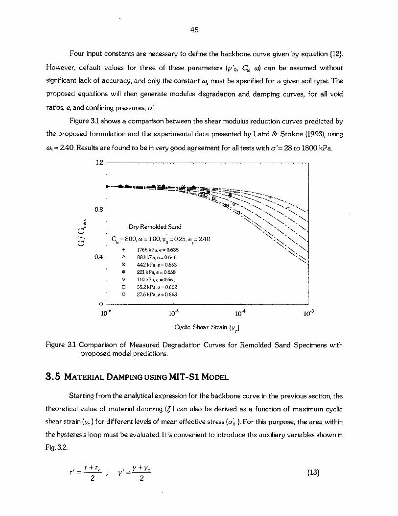
45
Four input constants are necessary to define the backbone curve given by equation {12}.
However, default values for three of these parameters (p'o, C, o) can be assumed without
significant lack of accuracy, and only the constant o, must be specified for a given soil type. The
proposed equations will then generate modulus degradation and damping curves, for all void
ratios, e, and confining pressures, c'.
Figure 3.1 shows a comparison between the shear modulus reduction curves predicted by
the proposed formulation and the experimental data presented by Laird & Stokoe (1993), using
ca 2.40. Results are found to be in very good agreement for all tests with a'= 28 to 1800 kPa.
1.2
0.8 -
E Dry Remolded Sand
C=80o, O=1.O, p =0.25,o =2.40
+ 1766 kPa, e = 0.6360.4 A 883 kPa, e =0.646
E 442 kPa, e = 0.653* 221 kPa, e = 0.658V 110 kPa, e = 0.6610 55.2 kPa, e = 0.662o 27.6 kPa, e = 0.663
0
10-6 10~5 104 103
Cyclic Shear Strain [y]
Figure 3.1 Comparison of Measured Degradation Curves for Remolded Sand Specimens withproposed model predictions.
3.5 MATERIAL DAMPING USING MIT-Si MODEL
Starting from the analytical expression for the backbone curve in the previous section, the
theoretical value of material damping ( ) can also be derived as a function of maximum cyclic
shear strain (yc) for different levels of mean effective stress (a' ). For this purpose, the area within
the hysteresis loop must be evaluated. It is convenient to introduce the auxiliary variables shown in
Fig. 3.2.
r I , y =C " Y +{13}2 2
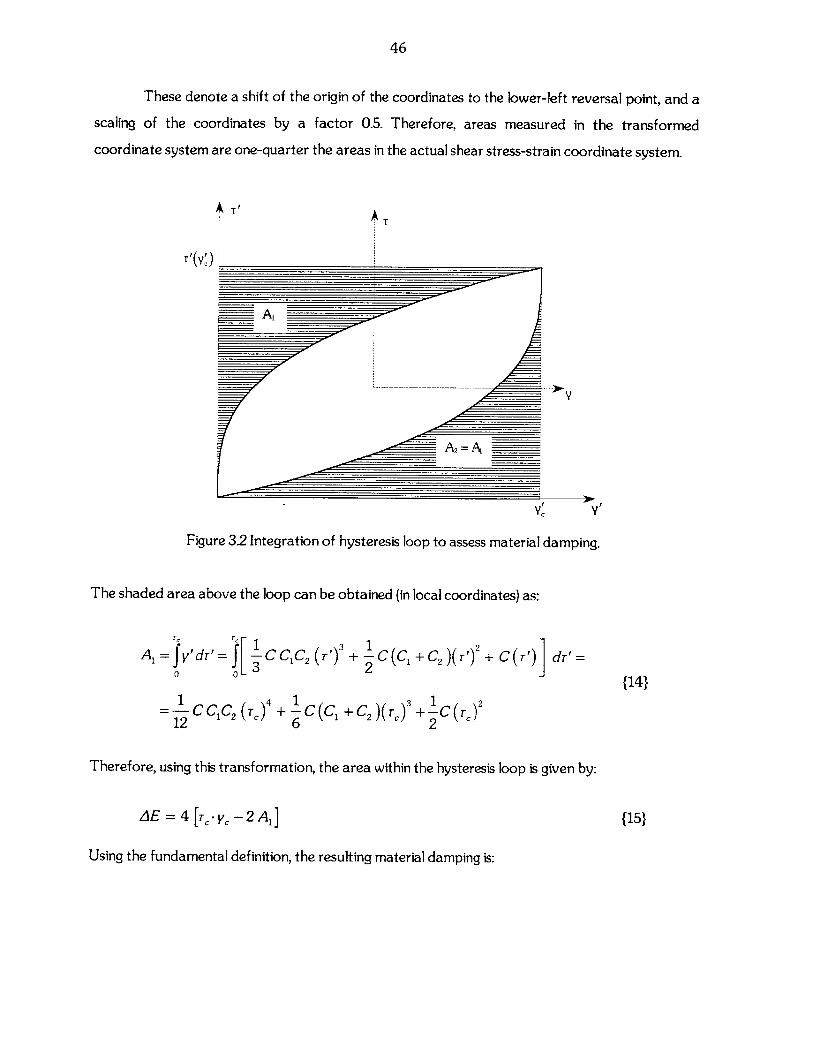
46
These denote a shift of the origin of the coordinates to the lower-left reversal point, and a
scaling of the coordinates by a factor 0.5. Therefore, areas measured in the transformed
coordinate system are one-quarter the areas in the actual shear stress-strain coordinate system.
AT'
r'(v')
TV
Figure 3.2 Integration of hysteresis loop to assess material damping.
The shaded area above the loop can be obtained (in local coordinates) as:
TC Tc~Al = y'dr' = f C CIC2 (rf') + C (Cl + C2 )(T ')2 + C (r')1 dr =4 ~1
0 1 0 1 31= C C1C 2 (re)4 + 1 C(C, + C2 )(T)3 +1C (rT) 2
12 6 2
Therefore, using this transformation, the area within the hysteresis loop is given by:
AE = 4 [rC -C -2 A1]
Using the fundamental definition, the resulting material damping is:
{14}
{15}
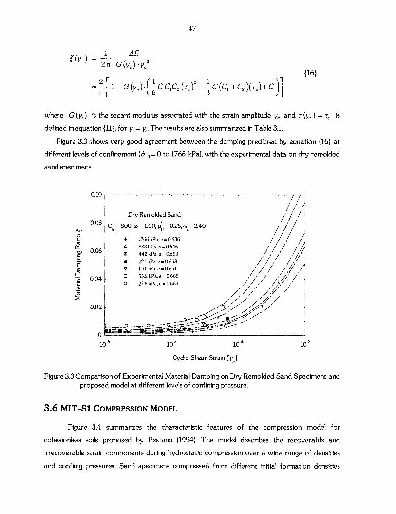
47
1 AE2rn G(yv)- y
2 12 +1=-1 -G(yc)- -CCC2(Te +-C(C1 +C2 )(re)+Cn- 6 3
{16}
where G (yc) is the secant modulus associated with the strain amplitude ye, and T (yc ) = re is
defined in equation {11}, for y = ye. The results are also summarized in Table 3.1.
Figure 3.3 shows very good agreement between the damping predicted by equation {16} at
different levels of confinement (o o= 0 to 1766 kPa), with the experimental data on dry remolded
sand specimens.
ct
0.
E
0.10
0.08
0.06
0.04
0.02
01
10 6
Cyclic Shear Strain [V ]
Figure 3.3 Comparison of Experimental Material Damping on Dry Remolded Sand Specimens andproposed model at different levels of confining pressure.
3.6 MIT-Si COMPRESSION MODEL
Figure 3.4 summarizes the characteristic features of the compression model for
cohesionless soils proposed by Pestana (1994). The model describes the recoverable and
irrecoverable strain components during hydrostatic compression over a wide range of densities
and confinig pressures. Sand specimens compressed from different initial formation densities
Dry Remolded Sand
C = 800, o =1.00, 1 =0.25, o,= 2.40
+ 1766 kPa, e = 0.636A 883 kPa, e = 0.646
9 442 kPa, e = 0.653G 221 kPa, e =0.658V 110 kPa, e = 0.6610 55.2 kPa, e = 0.662o 27.6 kPa, e = 0.663
--- --
10-5 10 -4 10-3
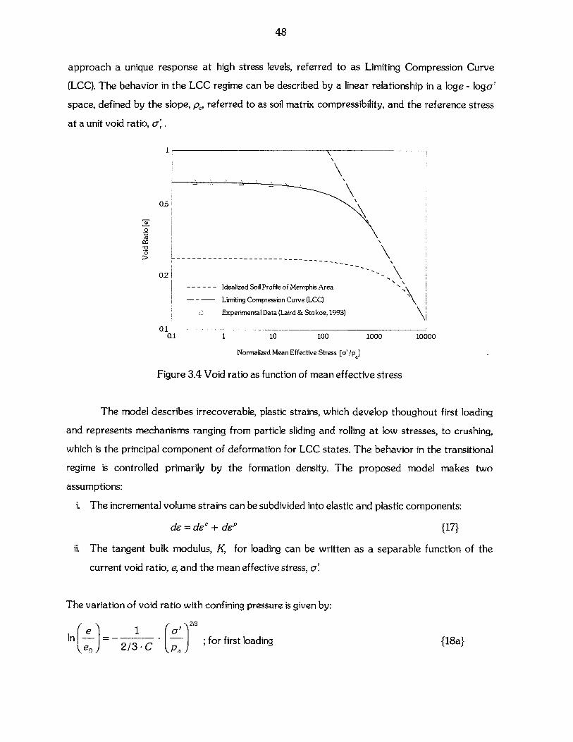
48
approach a unique response at high stress levels, referred to as Limiting Compression Curve
(LCC). The behavior in the LCC regime can be described by a linear relationship in a loge - logo'
space, defined by the slope, pc, referred to as soil matrix compressibility, and the reference stress
at a unit void ratio, a.
1
02
02L
- - - - - - Idealized Soil Profile of Memphis Area
- - -Limiting Compression Curve (LCC)
I Experimental Data (Laird & Stokoe, 1993)
0.10.1 1 10 100 1000 10000
Normalized Mean Effective Stress [a' /pj
Figure 3.4 Void ratio as function of mean effective stress
The model describes irrecoverable, plastic strains, which develop thoughout first loading
and represents mechanisms ranging from particle sliding and rolling at low stresses, to crushing,
which is the principal component of deformation for LCC states. The behavior in the transitional
regime is controlled primarily by the formation density. The proposed model makes two
assumptions:
i. The incremental volume strains can be subdivided into elastic and plastic components:
de = d" + de" {17}
ii. The tangent bulk modulus, K, for loading can be written as a separable function of the
current void ratio, e, and the mean effective stress, c'
The variation of void ratio with confining pressure is given by:
In (-e) = - ; for first loading {18a}e. 2/3 -C pa
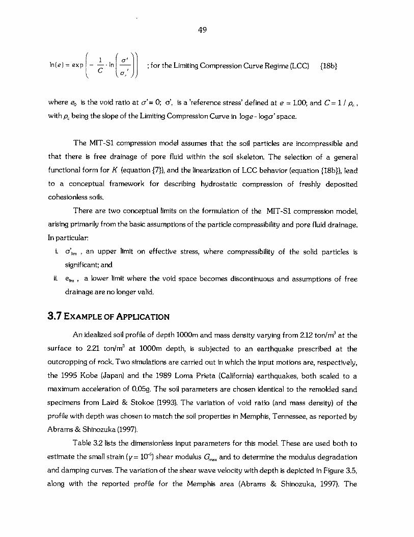
49
1 o-'In(e) = exp K h J , for the Limiting Compression Curve Regime (LCC) {18b}
where eo is the void ratio at o'= 0; 0', is a 'reference stress' defined at e = 1.00; and C = 1 / p,
with p, being the slope of the Limiting Compression Curve in loge - logo' space.
The MIT-Si compression model assumes that the soil particles are incompressible and
that there is free drainage of pore fluid within the soil skeleton. The selection of a general
functional form for K (equation {7}), and the linearization of LCC behavior (equation {18b}), lead
to a conceptual framework for describing hydrostatic compression of freshly deposited
cohesionless soils.
There are two conceptual limits on the formulation of the MIT-Si compression model,
arising primarily from the basic assumptions of the particle compressibility and pore fluid drainage.
In particular:
i. a', , an upper limit on effective stress, where compressibility of the solid particles is
significant; and
ii. elirn , a lower limit where the void space becomes discontinuous and assumptions of free
drainage are no longer valid.
3.7 EXAMPLE OF APPLICATION
An idealized soil profile of depth 1000m and mass density varying from 2.12 ton/rn3 at the
surface to 2.21 ton/m3 at 1000m depth, is subjected to an earthquake prescribed at the
outcropping of rock. Two simulations are carried out in which the input motions are, respectively,
the 1995 Kobe (Japan) and the 1989 Loma Prieta (California) earthquakes, both scaled to a
maximum acceleration of 0.05g. The soil parameters are chosen identical to the remolded sand
specimens from Laird & Stokoe (1993). The variation of void ratio (and mass density) of the
profile with depth was chosen to match the soil properties in Memphis, Tennessee, as reported by
Abrams & Shinozuka (1997).
Table 3.2 lists the dimensionless input parameters for this model. These are used both to
estimate the small strain (y = 10-6) shear modulus Gma. and to determine the modulus degradation
and damping curves. The variation of the shear wave velocity with depth is depicted in Figure 3.5,
along with the reported profile for the Memphis area (Abrams & Shinozuka, 1997). The
50
fundamental shear-beam frequency of the soil for this profile is 0.156 Hz, and there are some
twenty resonant modes in the 0-5 Hz frequency range.
Cb 800(a 1p'o 0.25WS 2.4eo 0.25
G'rev/ p a 6051C 2.26
Table 3.2 Input parameters for MIT-Si model
0
-200
-400
-600
-800
1000A
-c
200 400 600 800 1000
Shear Wave Velocity V, [m/sec]
Figure 3.5 Soil profile used for 1-D soil amplification simulation (measured data from Memphisarea by Abrams & Shinozuka, 1997)
The variation of void ratio with the mean effective stress is taken from the original
formulation for the MIT-Si model for cohesionless soils (Pestana & Whittle, 1995).
The dynamic response of the profile at the surface is calculated using the computer code
LAYSOL (Kausel, 1992), which is based on a continuum formulation of the wave propagation
problem in the frequency-wavenumber domain. The soil profile is divided into 100 homogeneous
layers of 10m thickness each, whose material properties are inferred from Fig. 3.5 (taking the
values at the center of the layers).
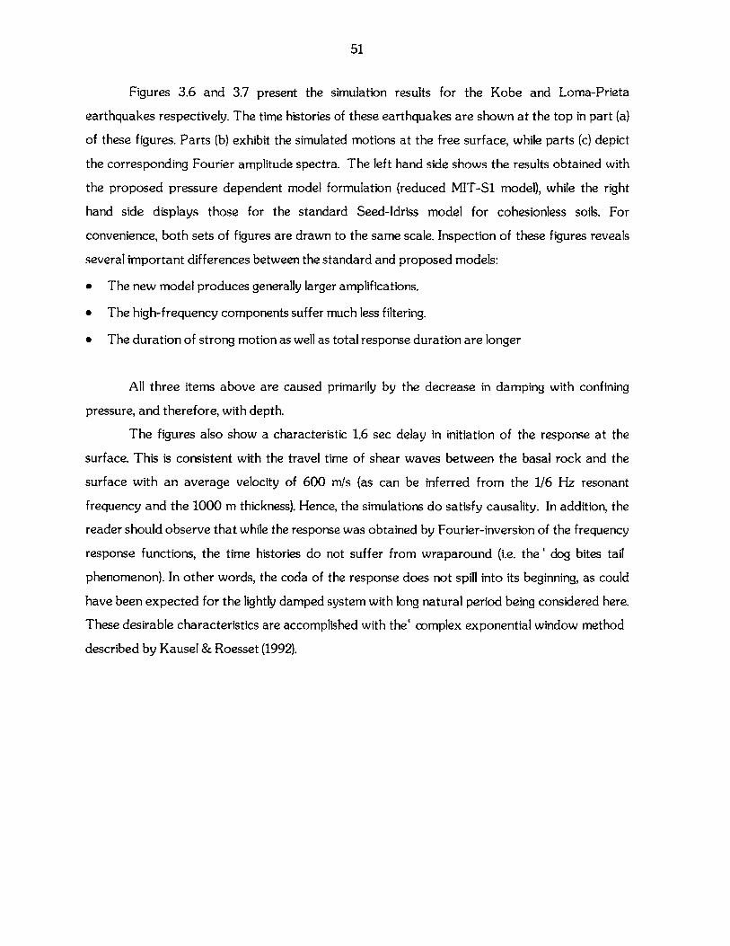
51
Figures 3.6 and 3.7 present the simulation results for the Kobe and Loma-Prieta
earthquakes respectively. The time histories of these earthquakes are shown at the top in part (a)
of these figures. Parts (b) exhibit the simulated motions at the free surface, while parts (c) depict
the corresponding Fourier amplitude spectra. The left hand side shows the results obtained with
the proposed pressure dependent model formulation (reduced MIT-Si model), while the right
hand side displays those for the standard Seed-Idriss model for cohesionless soils. For
convenience, both sets of figures are drawn to the same scale. Inspection of these figures reveals
several important differences between the standard and proposed models:
* The new model produces generally larger amplifications.
" The high-frequency components suffer much less filtering.
* The duration of strong motion as well as total response duration are longer
All three items above are caused primarily by the decrease in damping with confining
pressure, and therefore, with depth.
The figures also show a characteristic 1.6 sec delay in initiation of the response at the
surface. This is consistent with the travel time of shear waves between the basal rock and the
surface with an average velocity of 600 m/s (as can be inferred from the 1/6 Hz resonant
frequency and the 1000 m thickness). Hence, the simulations do satisfy causality. In addition, the
reader should observe that while the response was obtained by Fourier-inversion of the frequency
response functions, the time histories do not suffer from wraparound (i.e. the' dog bites tail
phenomenon). In other words, the coda of the response does not spill into its beginning, as could
have been expected for the lightly damped system with long natural period being considered here.
These desirable characteristics are accomplished with the' complex exponential window method
described by Kausel & Roesset (1992).
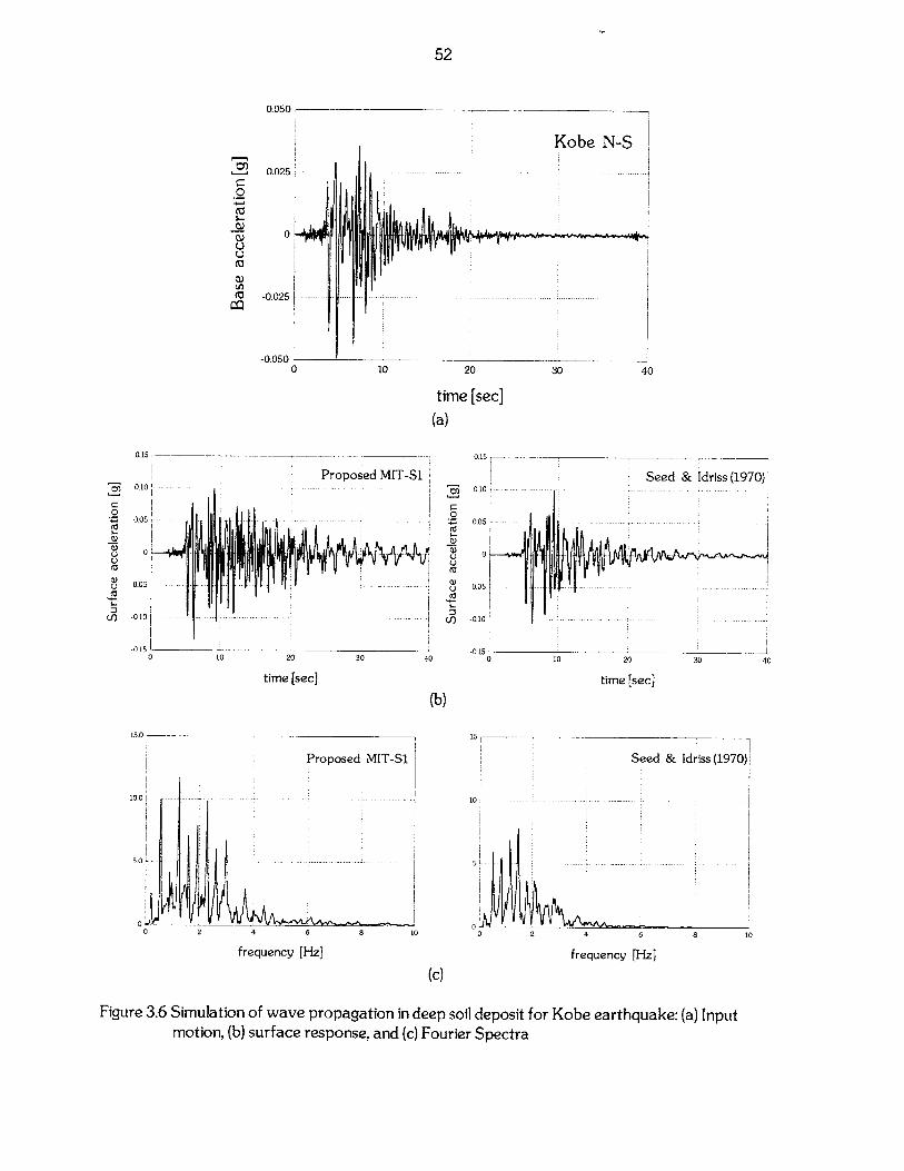
52
0.050
r-
UU
c)
(n
0.025.
0
-0.025
-0.050 L0
0.15 -
Proposed MIT-Si0.10
0.05 --- -
0
-0.05 -- ----
-0 -10 . .. ..- - -- - -- - -- -- - - -
0.1510 20 30
time [sec]
-0-15J40 0 10 20 30
time [sec]
(b)
Proposed MIT-Si
10
5
6 2
frequency [Hz]
(c)
Figure 3.6 Simulation of wave propagation in deep soil deposit formotion, (b) surface response, and (c) Fourier Spectra
Seed & Idriss (1970)i
4 6
frequency [Hz]
Kobe earthquake: (a) Input
Kobe N-S
10 20 30
time (sec](a)
40
C
0)0)
U.
0-15
0.10
0.05
0
-0.05
-0.10
0
U
V)
40
15.0
100
5.0
010
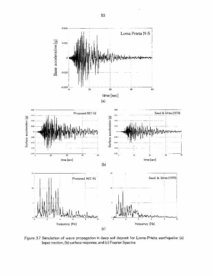
53
0.050
Loma Prieta N-S
25
0
25 - - - - --
-0.0500 10 20
time [sec]
(a)
30
Proposed MIT-Si
-- -- -
0
30 40
0201-
015
0.10
0.05
0-
-0.05
-0.10
-0.15
-020 L0
Seed & Idriss (1970)-- -----
- - - ---
-.. ... ---- --- ------ -
10 20
time [sec]
30 40
(b)
Proposed MIT-Si Seed & Idriss (1970)1
10 - - - - --
5,
2 4 6
frequency [Hz]
10 2
frequency [Hz]
(c)
Figure 3.7 Simulation of wave propagation in deep soil deposit for Loma-Prieta earthquake: (a)Input motion, (b) surface response, and (c) Fourier Spectra
0.0
(a(-
W
M
-0.0
0,
Q)
U)
020
015
0.10
0.05
0 ~-0.05
-0.10
-0.15
-0.20-0
-r rr 1IR llI?
10
time [sec]
10
10
I
40
54
3.8 CONCLUSIONS
This chapter presented a simple four-parameter model for the dynamic shear moduli and
damping characteristics of granular soils when they deform in shear only. This model is based on
the MIT-Si generalized plasticity model proposed earlier by Pestana and Whittle (1995). Its four
parameters can readily be measured in the laboratory, or estimated from existing data. The shear
moduli and damping values predicted by the proposed model were found to be in excellent
agreement with experimental results obtained by Laird and Stokoe (1993) over a wide range of
confining pressures.
The proposed formulation takes into account the effect of confining pressure on soil
parameters and hysteretic behavior, and therefore, permits proper consideration of the hysteretic
characteristics of the ground with depth. As demonstrated with two simulations for a 1 km deep
site, the dependence of the dynamic moduli on confining pressure can be an important
consideration in the analysis of soil deposits for earthquake effects.
The simulations indicate that when the confining pressure is taken into account, the
elasticity of the soil steadily increases with depth. The refinement introduced by the pressure-
dependant characterization of the soil in turn alleviates significantly one of the alleged
shortcomings of the standard equivalent-linear model, which is that it unrealistically wipes out the
high-frequency components of motion when used for moderately deep to very deep soil profiles.
3.9 REFERENCES
Abrams, D.P. & Shinozuka, M. (1997)." Loss Assessment of Memphis Buildings , Technical ReportNCEER-97-0018.
Constantopoulos, I.V., Roesset, J.M. & Christian, J.T. (1973). "A comparison of linear and nonlinearanalyses of soil amplification". 5th World Conference on Earthquake Engineering, Rome
Dobry, R., Ladd, R.S., Yokel, F.Y., Chung, R.M. & Powell, D. (1982). "Prediction of pore waterpressure buildup and liquefaction of sands during earthquakes using the cyclic strain method",NBS Building Science Series 138, National Bureau of Standards, Gaithersburg, Maryland
Hardin, B. 0. (1965). "The nature of damping in sands", Journal of Soil Mechanics andFoundation Engineering Division, ASCE, Vol. 91, No. SM1, February, pp. 33-65.
Hardin, B. 0. & Drnevich, V. P. (1970)." Shear modulus and damping in soils: I. Measurement andparameter effects, II. Design equations and curves , Technical Reports UKY 27-70-CE 2and 3, College of Engineering, University of Kentucky, Lexington, Kentucky.
Hardin, B. 0. & Drnevich, V. P. (1972a)." Shear modulus and damping in soils: Measurement andparameter effects ,Journal of Soil Mechanics and Foundation Engineering Division, ASCE,Vol. 98, No. SM6, June, pp. 603-624.
55
Hardin, B. 0. & Drnevich, V. P. (1972b)." Shear modulus and damping in soils: Design equations andcurves , Journal of Soil Mechanics and Foundation Engineering Division, ASCE, Vol. 98,No. SM7, pp. 667-692.
Houlsby, G.T. (1965).'" The use of a Variable Shear Modulus in Elastic-Plastic Models for Clays',Computers and Geotechnics, Vol.1, No.1, pp. 3-21.
Iwasaki, T., Tatsuoka, F. & Takagi, Y. (1978). "Shear Moduli of Sands under Cyclic TorsionalShear Loading", Soils and Foundations, Vol. 18, No.1, pp. 39-56.
Jaky, J. (1948). "Pressure in Silos", 2nd ICSMFE, Vol.1, pp. 103-107.Kausel, E. (1992)." LAYSOL: A computer program for the dynamic analysis of layered soils'.Kausel, E. and Roesset, J.M. (1992)." Frequency domain analysis of undamped systems , Journal of
Engineering. Mechanics, ASCE, 118 (4), pp. 721-734Lade, P.V. & Nelson, R.B. (1987)." Modeling the Elastic Behavior of Antigranulocytes-Materials' ,
International Journal for Numerical and Analytical Methods in Geomechanics, Vol. 11, No.5, pp. 521-542.
Laird, J. P. & Stokoe, K. H. (1993)." Dynamic properties of remolded and undisturbed soil samplestested at high confining pressure ', Geotechnical Engineering Report GR93-6, ElectricalPower Research Institute.
Loret, B. & Luong, M.P. (1982)." Double Deformation Mechanism for Sand' , Proc. 4th Int. Conf.Num. Meth. and Advances in Geomechanics, Edmonton, Alberta.
Mesri, G. & Hayat, T.M. (1993). "The Coefficient of Earth Pressure at Rest", CGJ, Vol. 30, No. 4,August, pp. 647-666.
Ng T.T. & Dobry, R. (1992)." A Non-linear Numerical Model for Soil Mechanics' , InternationalJournal for Numerical and Analytical Methods in Geomechanics, Vol. 16, No. 4, pp. 247-263.
Ng T.T. & Dobry, R. (1994)." Numerical Simulations of Monotonic and Cyclic Loading of GranularSoil', Journal of Geotechnical Engineering, ASCE, Vol. 120, No. 2, pp. 388-403.
Civil Engineering, University of Texas at Austin, August.Pestana, J.M. (1994)." A unified constitutive model for sands and clays , ScD Thesis, Department
of Civil Engineering, Massachusetts Institute of Technology.Pestana, J. M. & Whittle, A. J. (1994)." Model Prediction of Anisotropic Clay Behavior due to
Consolidation Stress History' , Proc. 8th Int. Conf Comp. Meth. and Advances inGeomechanics, Morgantown, Virginia.
Pestana, J. M. & Whittle, A. J. (1995)." Predicted effects of confining stress and density on shearbehavior of sand', Proc. 4th Int. Conf Computational Plasticity, Barcelona (Spain), 2, pp.2319-2330.
Pestana, J. M. & Whittle, A. J. (1995)." Compression model for cohesionless soils" Geotechnique45, (4), pp. 611-631.
Shibata, T. & Soelarno, D. S. (1975)," Stress strain characteristics of sands under cyclic loading',Proc.. Japanese Society of Civil Engineering, 239, pp. 57-65.
Whittle, A.J. (1987), "A constitutive model for Overconsolidated Clays with Application to theCyclic Loading of Friction Piles", Sc. M. Thesis, MIT, Cambridge, MA
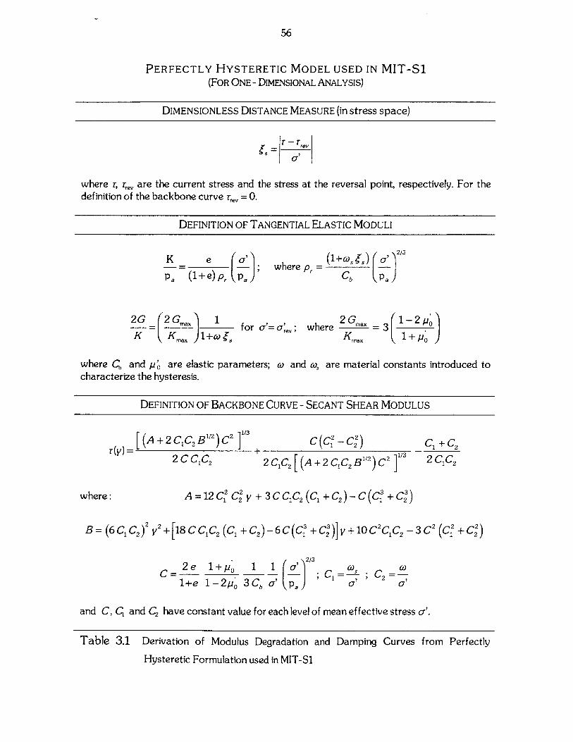
56
PERFECTLY HYSTERETIC MODEL USED IN MIT-Si(FOR ONE - DIMENSIONAL ANALYSIS)
DIMENSIONLESS DISTANCE MEASURE (in stress space)
= Trev
where , r, are the current stress and the stress at the reversal point, respectively. For thedefinition of the backbone curve Trev =0.
DEFINITION OF TANGENTIAL ELASTIC MODULI
K -e ( ; where pr = (i+6) 5 rz'5 )2 3
p, (1+e)p, pa' Cb (Pa
2G 2G 1- "m" for c'= c'.;K K. 1 +o , re
where m" = 3 ,Kma 1+ P0
where Cq and p' are elastic parameters; o and o, are material constants introduced tocharacterize the hysteresis.
DEFINITION OF BACKBONE CURVE - SECANT SHEAR MODULUS
(A +2C 1 C2 B112 )C 2 ]1/3
2CCC 2+
C(C2 -C2)
2 C1C2 [(A + 2 C1C2Bz112) C2 11/3
where: A=12C C2y + 3CC1 C2 (C+C 2 )-C(C3 +C2)
B= (6C1 C22 2+[18 C C1 C2 (C +C 2 )-6C(Cf +Cl)]y+10C2C1C2 -3C 2 (Cf +Cl)
0 =2e 1+po 1 11+e 1-2po 3 Cb c
-- ; C 1 = ";C 2 =-(p, a a
and C, C and C2 have constant value for each level of mean effective stress a'.
Table 3.1 Derivation of Modulus Degradation and Damping Curves from Perfectly
Hysteretic Formulation used in MIT-Si
C1+C2
2C1C2
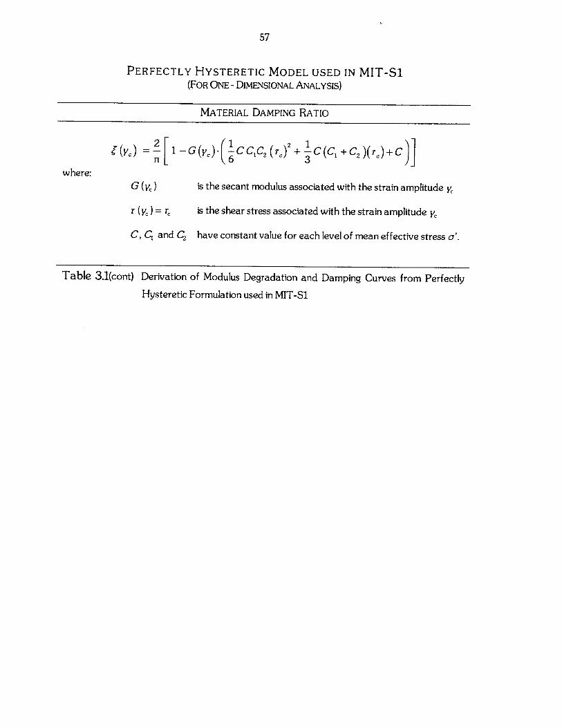
57
PERFECTLY HYSTERETIC MODEL USED IN MIT-Sl(FOR ONE - DIMENSIONAL ANALYSIS)
MATERIAL DAMPING RATIO
S(yj) 1 -G(y,)- C CIC2 (rej2 + -C (C + C, )(re + C
where:G (ye) is the secant modulus associated with the strain amplitude ye
r (yc) = rc is the shear stress associated with the strain amplitude yc
C, C and C2 have constant value for each level of mean effective stress c'.
Table 3.1(cont) Derivation of Modulus Degradation and Damping Curves from Perfectly
Hysteretic Formulation used in MIT-Si
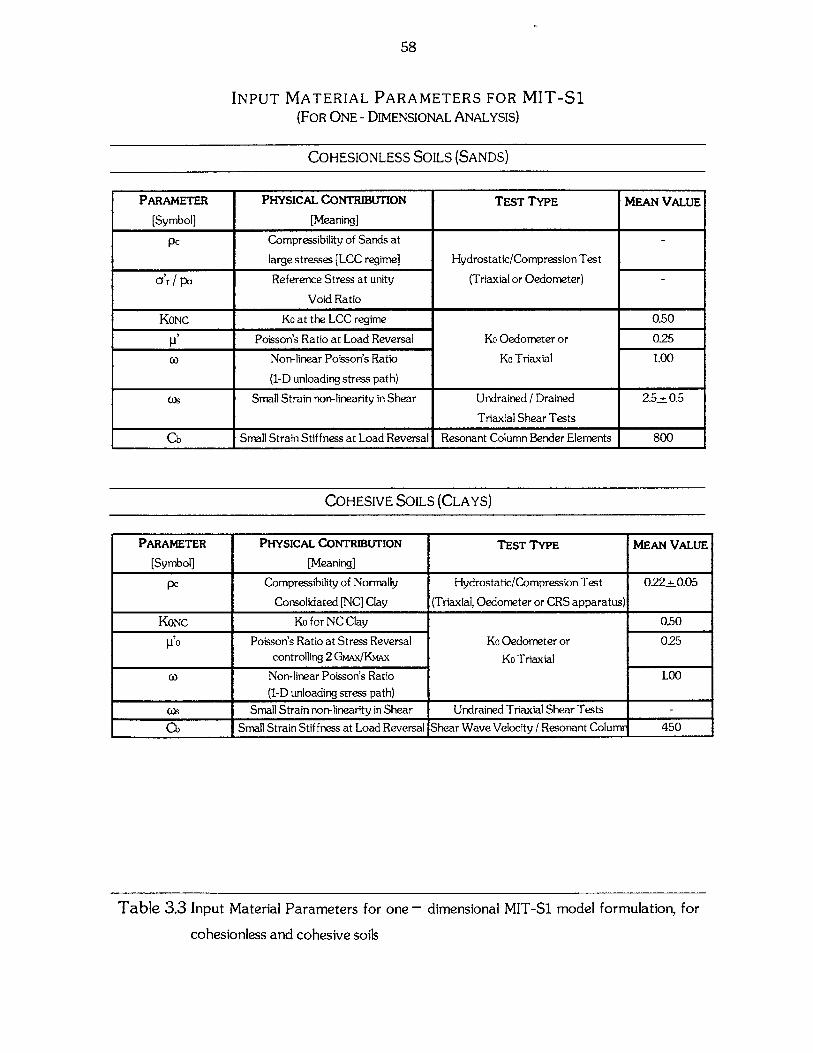
58
INPUT MATERIAL PARAMETERS FOR MIT-Si(FOR ONE - DIMENSIONAL ANALYSIS)
COHESIONLESS SOILS (SANDS)
PARAMETER PHYSICAL CONTRIBUTION TEST TYPE MEAN VALUE
[Symbol] [Meaning]
PC Compressibility of Sands at
large stresses [LCC regime] Hydrostatic/Compression Test
O'r / pa Reference Stress at unity (Triaxial or Oedometer) -
Void Ratio
KONC Ko at the LCC regime 0.50
p' Poisson's Ratio at Load Reversal Ko Oedometer or 0.25
O Non-linear Poisson's Ratio Ko Triaxial 1.00
(1-D unloading stress path)
Cos Small Strain non-linearity in Shear Undrained / Drained 2.5- 0.5
Triaxial Shear Tests
Cb Small Strain Stiffness at Load Reversal Resonant Column Bender Elements 800
COHESIVE SOILS (CLAYS)
PARAMETER PHYSICAL CONTRIBUTION TEST TYPE MEAN VALUE
[Symbol] [Meaning]
pc Compressibility of Normally Hydrostatic/Compression Test 022±0.05
Consolidated [NC] Clay (Triaxial, Oedometer or CRS apparatus)
KONc Ko for NC Clay 0.50
P Poisson's Ratio at Stress Reversal Ko Oedometer or 025
controlling 2 GMAx/KMAx Ko Triaxial
o Non-linear Poisson's Ratio 100
(1-D unloading stress path)
os Small Strain non-linearity in Shear Undrained Triaxial Shear Tests -
Cb Small Strain Stiffness at Load Reversal Shear Wave Velocity / Resonant Columr 450
Table 3.3 Input Material Parameters for one - dimensional MIT-Si model formulation, for
cohesionless and cohesive soils
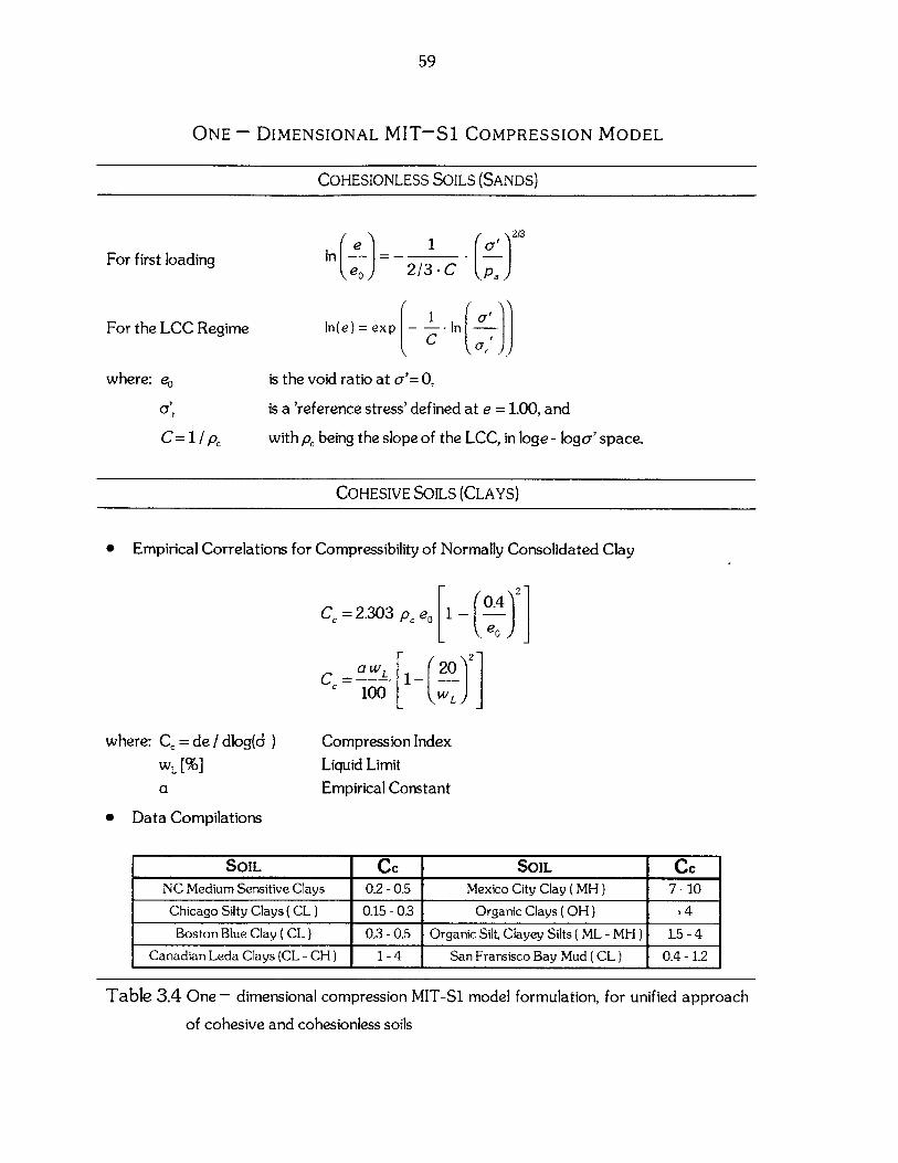
59
ONE - DIMENSIONAL MIT-Si COMPRESSION MODEL
COHESIONLESS SOILS (SANDS)
For first loading
For the LCC Regime
where: eo
a' r
C=1/pc
In(e )= 1 - c')2
eo 2/3-C p,,
CJ 1 'In(e)= exp In
C C,
is the void ratio at o'= 0,
is a 'reference stress' defined at e =1.00, and
with pc being the slope of the LCC, in loge - loga'space.
COHESIVE SOILS (CLAYS)
* Empirical Correlations for Compressibility of Normally Consolidated Clay
C = 2.303 p, eo [1 - 04J1
2
awL 1_ 202
100 [ w
where: Ce = de / dlog(d)
WL [%]a
* Data Compilations
Compression Index
Liquid Limit
Empirical Constant
SOIL Cc SOIL CcNC Medium Sensitive Clays 0.2 - 0.5 Mexico City Clay (MH) 7-10
Chicago Silty Clays ( CL) 0.15 -0.3 Organic Clays ( OH) ) 4
Boston Blue Clay ( CL) 0.3 - 0.5 Organic Silt, Clayey Silts ( ML - MH) 1.5-4
Canadian Leda Clays (CL - CH) 1-4 San Fransisco Bay Mud ( CL) 0.4 - 1.2
Table 3.4 One - dimensional compression MIT-Si model formulation, for unified approach
of cohesive and cohesionless soils

60
61
CHAPTER 4
REPRESENTATION OF STRESS - STRAIN RELATIONS
IN CYCLIc LOADING
4.1 INTRODUCTION
Soils do not exhibit linear elastic behavior except at very small strains (less than 10-5, ingeneral). In this range the nonlinear effects while present, have little influence and can hardly be
assessed because it is difficult to measure such small strains and stresses accurately.
At larger strains, such as the ones induced by relatively strong earthquakes,experimental data (Hardin & Drnevich, 1972a, 1972b; Seed & Idriss, 1969; Thiers & Seed,1968) show that the stress-strain relationships for soils deviate from linearity, and, therefore,nonlinear effects cannot be ignored. Certain features of this relationship, whilst complicated,can be identified from available experimental data:
i. The hysteretic stress stress-strain behavior of soils is nonlinear and strain-dependent.
ii. The loops exhibit a sudden change in slope when the strain changes direction.
iii. The unloading and reloading branches of the loops appear geometrically similar when
measured from the reversal point of strain.
iv. The tangent modulus upon reversal of strain is approximately the same for both the
unloading and reloading parts of the loop, and is approximately equal to the initial
modulus.
v. The area enclosed by each loop is the energy loss per cycle, and is independent of strain
rate.
Modeling of soil behavior under cyclic or random loading conditions may be made so
that the model can duplicate the deformation characteristics in the range of strains under
consideration. When soil behavior is expected to stay within the small strain range (i.e. below
the elastic threshold), the use of an elastic model is justified and the shear modulus is a key
parameter to properly model the soil behavior.
When a given problem is associated with the medium range of strain, approximately
below the level of 10-, the soil behavior becomes elastoplastic and the shear modulus tends to
62
decrease as the shear strain increases. At the same time, energy dissipation occurs during
cycles of load application. The energy dissipation in soils is mostly rate - independent and of
hysteretic nature, and the damping ratio can be used to represent the energy absorbing
properties of soils. Since the strain level concerned is still small enough not to cause any
progressive change in soil properties, the shear modulus and damping ratio do not change with
the progression of cycles in load application. This kind of behavior is called non-degraded
hysteresis type. Such steady-stage soil characteristics can be represented to a reasonable
degree of accuracy by use of the linear viscoelastic theory. The shear modulus and damping
ratio, determined as functions of shear strain, are the key parameters to represent soil
properties in this medium strain range. The most useful analytical tool accommodating these
strain - dependent but cycle - independent soil properties would be the equivalent linear
method based on the viscoelastic concept. Generally, the linear analysis is repeated, by
stepwise changing the soil parameters until a strain - compatible solution is obtained. The
seismic response analysis performed for horizontally layered soil by use of the computer
program SHAKE (Schnabel et al., 1972) is a typical example of an analytical tool that can be
successfully used to clarify the soil response in the medium range of strain.
For the shear strain level larger than about 10-2, soil properties tend to change
appreciably not only with shear strain but also with the progression of cycles. This kind of
behavior is termed degraded hysteresis type. The manner in which the shear modulus and
damping change with cycles is considered to depend upon the manner of change in the
effective confining stress during irregular time histories of shear stress application. When the
law of changing effective stress is established, it is then necessary to have constitutive law in
which stress - strain relations can be specified at each step of loading, unloading and reloading
phases. One of the concepts most commonly used at present for this purpose is what is
referred to as the Masing law. For analysis of a soil response accommodating such a stress -
strain law covering large strain levels near failure, it is necessary to employ a numerical
procedure involving the step - by - step integration technique.
In what follows, the methods of modeling soil behavior will be discussed and the soil
model used for the present analysis will be described.
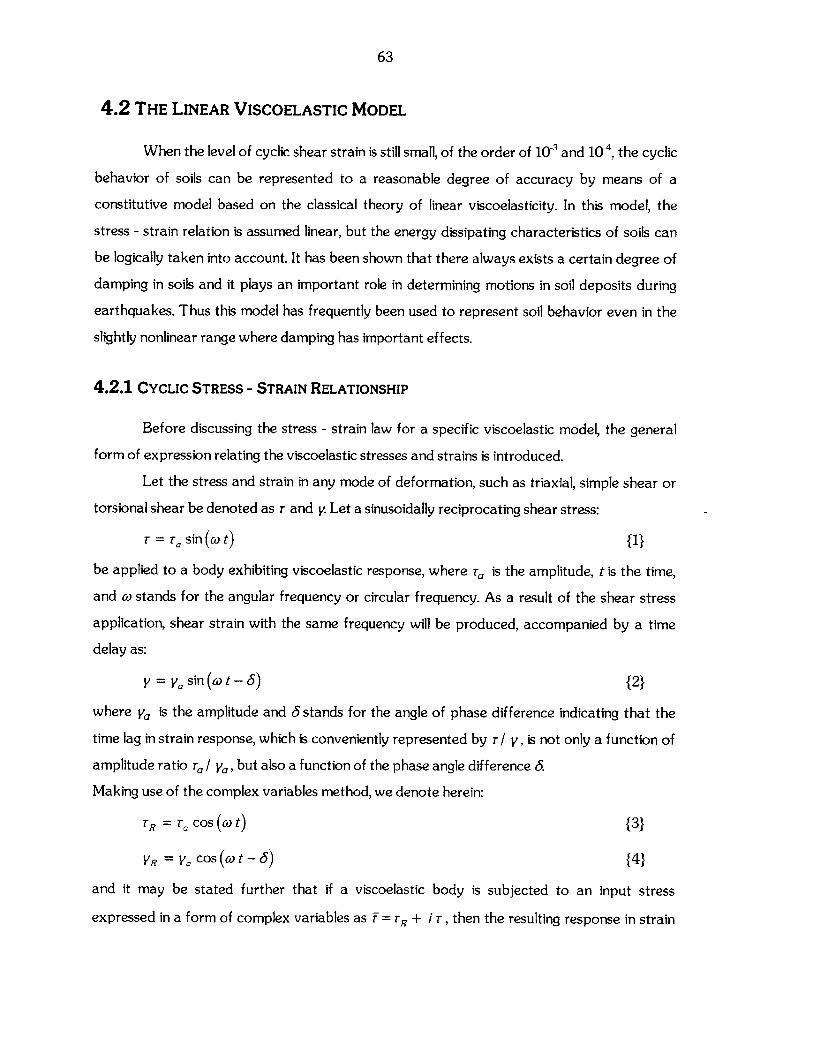
63
4.2 THE LINEAR VISCOELASTIC MODEL
When the level of cyclic shear strain is still small, of the order of 10-3 and 10-4, the cyclic
behavior of soils can be represented to a reasonable degree of accuracy by means of a
constitutive model based on the classical theory of linear viscoelasticity. In this model, the
stress - strain relation is assumed linear, but the energy dissipating characteristics of soils can
be logically taken into account. It has been shown that there always exists a certain degree of
damping in soils and it plays an important role in determining motions in soil deposits during
earthquakes. Thus this model has frequently been used to represent soil behavior even in the
slightly nonlinear range where damping has important effects.
4.2.1 CYCLIC STRESS - STRAIN RELATIONSHIP
Before discussing the stress - strain law for a specific viscoelastic model, the general
form of expression relating the viscoelastic stresses and strains is introduced.
Let the stress and strain in any mode of deformation, such as triaxial, simple shear or
torsional shear be denoted as r and y. Let a sinusoidally reciprocating shear stress:
T = rasin (o t) {1}
be applied to a body exhibiting viscoelastic response, where ra is the amplitude, t is the time,
and co stands for the angular frequency or circular frequency. As a result of the shear stress
application, shear strain with the same frequency will be produced, accompanied by a time
delay as:
y = ya sin(t t -6) {2}
where y is the amplitude and 6 stands for the angle of phase difference indicating that the
time lag in strain response, which is conveniently represented by r / y, is not only a function of
amplitude ratio Ta / ya, but also a function of the phase angle difference 6.
Making use of the complex variables method, we denote herein:
TR = Ta cos (co t) {3}
YR = y, cos (o t -6) {4}
and it may be stated further that if a viscoelastic body is subjected to an input stress
expressed in a form of complex variables as r= TR + i r, then the resulting response in strain
64
would be V= YR + i V , where i is the unit imaginary number and T and y are the stress and
strain in complex variables. We therefore have:
S=T re e''' {5}
y = Va e {6}
The strain versus stress response can be described by the ratio T*/ , which is explicitly written
as:
T rT- = -"-e' = -"-(cos6+isin)=p+i p=p {7}V ya Ya
where p and p'are called elastic modulus and loss modulus, respectively, and p' is named
complex modulus. The elastic modulus is a parameter indicative of elastic or instantaneous
power and loss modulus represents the energy dissipating characteristics of the viscoelastic.
Finally we have:
Va=a M, 2+p2 -18a}
tan 3= =n {8b}p
where n is a parameter called loss coefficient which is indicative of energy loss or damping
characteristics. From equation {8a} and {8b}, the absolute value of the complex modulus p* is
shown to indicate the shear modulus of the material.
It is to be noted here that the material parameters p and p'need not necessarily be real
constants, but could be a function of the angular frequency co. Therefore the moduli P and p'
as defined in equation {7} are regarded as the most general expression, and consequently can
take any form expressed as a function of frequency. Once a functional form is specified to
these moduli, the viscoelastic behavior of the material can be described in a more tangible
manner. Several methods for specifying these moduli have been proposed, either on the basis
of direct experiments or on the basis of spring-dashpot models.
4.2.2 HYSTERETIC STRESS - STRAIN CURVE
Describing the stress - strain behavior of a viscoelastic body, the pair of equations {1}and {2} can be viewed as a stress - strain relation, correlated through a tracking parameter cot.
Therefore, by eliminating the parameter cot, a single relation as follows is obtained:
65
- 2 cos + - sin2C5=0 {9}ra Y, ra y"
This is regarded as a second order equation with respect to r / r. Solving with
reference to the definition of p and p' one obtains:
r=/JYp' Ya y {10}
An alternative expression is obtained by decomposing the right - hand side of
equation {10} in two parts, namely:
T =T 1 +TF 2
7I =Ip V {11}
T2 2 + (If =1p Va Ya
-Therefore, the actual value of shear stress can be graphically represented as the
addition of a straight line with slope p (r) and an ellipse (r2 ). The result of this manipulation is
an ellipse with inclined axis, as shown in Fig. 4.1.
As indicated in Fig. 4.1, the inclined ellipse cut the ordinate at a shear stress point of
p'-y . Therefore, the value of p' may be taken as a measure to indicate a degree of flatness in
the shape of the ellipse. The greater the value of A , the rounder the ellipse indicating that the
energy loss or damping is bigger, whereas the smaller the value of p' ,the thinner the ellipse and,
hence, the smaller the damping during cyclic loading.
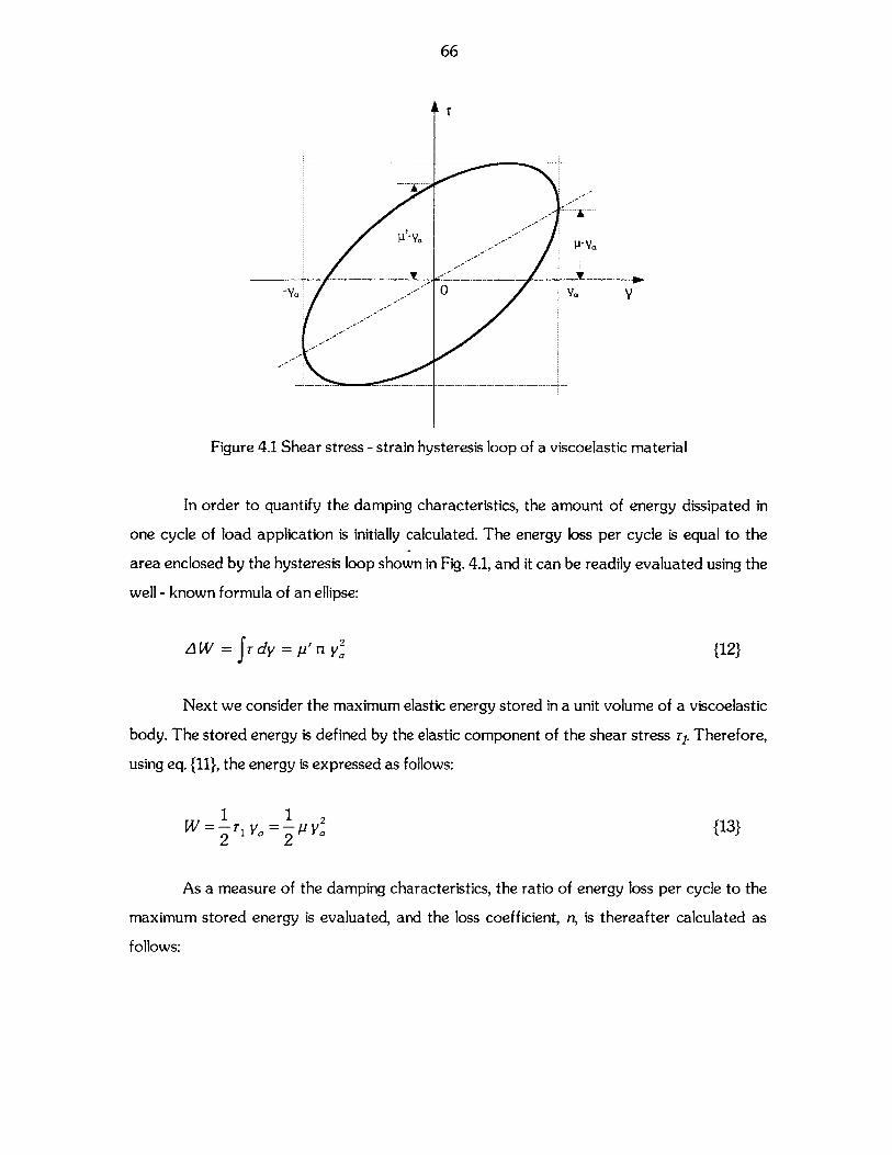
66
T
y
Figure 4.1 Shear stress - strain hysteresis loop of a viscoelastic material
In order to quantify the damping characteristics, the amount of energy dissipated in
one cycle of load application is initially calculated. The energy loss per cycle is equal to the
area enclosed by the hysteresis loop shown in Fig. 4.1, and it can be readily evaluated using the
well - known formula of an ellipse:
AW = frdy = p' ny2 {12}
Next we consider the maximum elastic energy stored in a unit volume of a viscoelastic
body. The stored energy is defined by the elastic component of the shear stress r1. Therefore,
using eq. {11}, the energy is expressed as follows:
1 12W = - Ti Y, = - P ya {13}
2 2
As a measure of the damping characteristics, the ratio of energy loss per cycle to the
maximum stored energy is evaluated, and the loss coefficient, n, is thereafter calculated as
follows:
-- ------- --------------
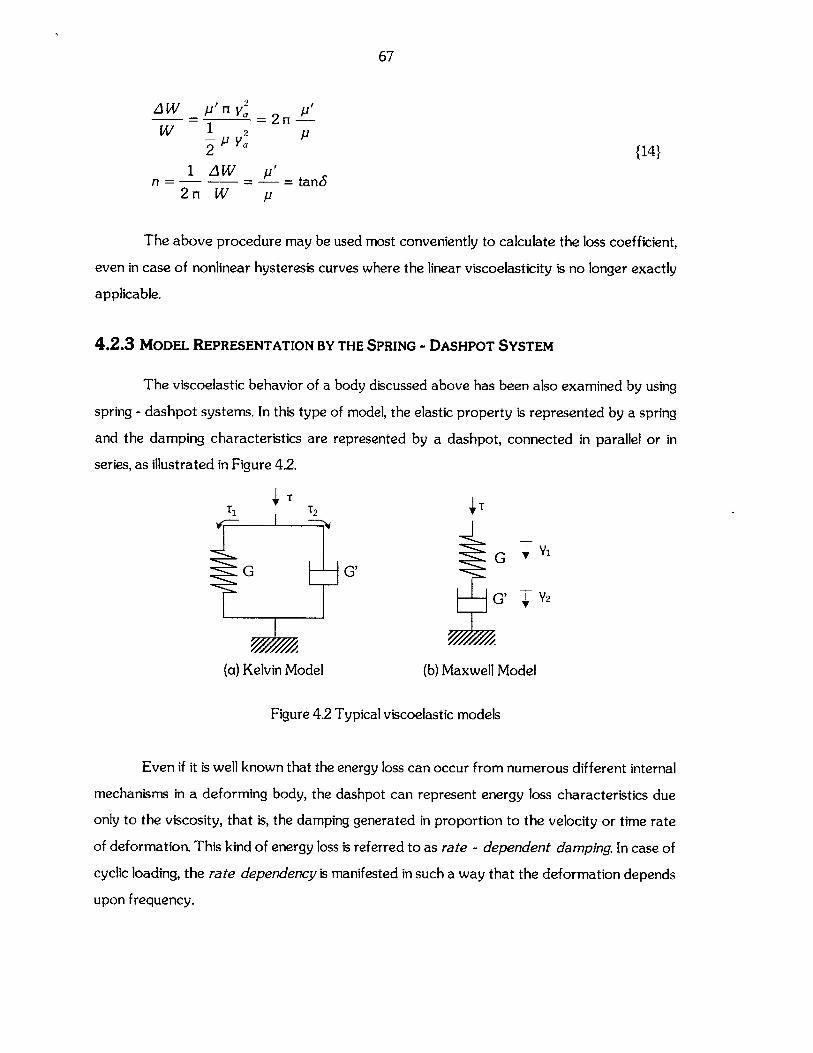
67
2'W- P, n y, = 2,1L
W 1 2 P2 P V {14}
1lAW p'n - = --- = tan3
2rn W p
The above procedure may be used most conveniently to calculate the loss coefficient,
even in case of nonlinear hysteresis curves where the linear viscoelasticity is no longer exactly
applicable.
4.2.3 MODEL REPRESENTATION BY THE SPRING - DASHPOT SYSTEM
The viscoelastic behavior of a body discussed above has been also examined by using
spring - dashpot systems. In this type of model, the elastic property is represented by a spring
and the damping characteristics are represented by a dashpot, connected in parallel or in
series, as illustrated in Figure 4.2.
G 4 VG G'
G' 47V2
(a) Kelvin Model (b) Maxwell Model
Figure 4.2 Typical viscoelastic models
Even if it is well known that the energy loss can occur from numerous different internal
mechanisms in a deforming body, the dashpot can represent energy loss characteristics due
only to the viscosity, that is, the damping generated in proportion to the velocity or time rate
of deformation. This kind of energy loss is referred to as rate - dependent damping. In case of
cyclic loading, the rate dependency is manifested in such a way that the deformation depends
upon frequency.
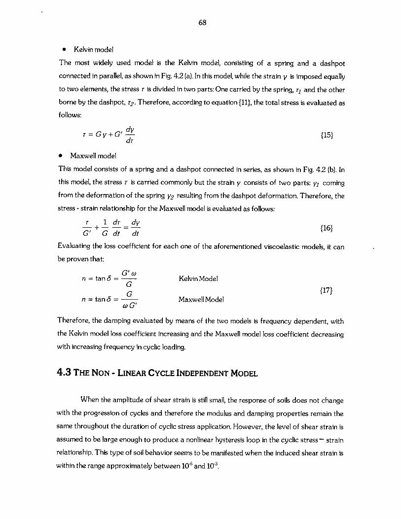
68
* Kelvin model
The most widely used model is the Kelvin model, consisting of a spring and a dashpot
connected in parallel, as shown in Fig. 4.2 (a). In this model, while the strain y is imposed equally
to two elements, the stress r is divided in two parts: One carried by the spring, r and the other
borne by the dashpot, r2 .Therefore, according to equation {11}, the total stress is evaluated as
follows:
r =Gy+G' dT {15}dr
* Maxwell model
This model consists of a spring and a dashpot connected in series, as shown in Fig. 4.2 (b). In
this model, the stress r is carried commonly but the strain y consists of two parts: V coming
from the deformation of the spring V2 resulting from the dashpot deformation. Therefore, the
stress - strain relationship for the Maxwell model is evaluated as follows:
r 1 dT dy- + - -= - {16}G' G dt dt
Evaluating the loss coefficient for each one of the aforementioned viscoelastic models, it can
be proven that:
n = tan 3 = G' o Kelvin ModelG
n = tan 6 = G Maxwell Modelco G'
Therefore, the damping evaluated by means of the two models is frequency dependent, with
the Kelvin model loss coefficient increasing and the Maxwell model loss coefficient decreasing
with increasing frequency in cyclic loading.
4.3 THE NON - LINEAR CYCLE INDEPENDENT MODEL
When the amplitude of shear strain is still small, the response of soils does not change
with the progression of cycles and therefore the modulus and damping properties remain the
same throughout the duration of cyclic stress application. However, the level of shear strain is
assumed to be large enough to produce a nonlinear hysteresis loop in the cyclic stress - strain
relationship. This type of soil behavior seems to be manifested when the induced shear strain is
within the range approximately between 10-5 and 10-3.
69
Modeling the stress - strain nonlinear soil behavior, two types of curves need to be
specified. In particular, one is associated with monotonic loading and the other constitutes a
cyclic loop. The former is referred to as backbone curve or skeleton curve and the latter is
called a hysteresis loop. As an extension to the nonlinear case, it may be mentioned that the
skeleton curve and the hysteresis loop indicate respectively, the elastic property and energy
dissipating characteristics, which are nonlinear. Due to this feature, the skeleton curve is not a
straight line nor does the hysteresis loop have rounded corners.
In constructing a nonlinear cyclic stress- strain relation, two basic functions need to be
specified, one for the backbone curve and the other for the hysteresis loop. The backbone
curve can be expressed by the following relationship:
T = f( y) {18}
which is obtained from monotonic loading tests on soils. For the load reversal occurring at
point (ya, Ta ), the equation of the stress- strain curve for the subsequent unloading is given as:
T-T y-y_ {9"2 f " {19}
2 k2)
The unloading branch of the stress - strain curve as defined above implies that a half
part of the hysteresis curve is obtained by two - fold stretching of the skeleton curve and by
translating its one end to the point of the stress reversal. Similarly, for reloading occurring at
point (- ya,,- Ta), the stress - strain curve for the reloading branch is now given by:
r + r y+T = fj " {20}
It is shown that the reloading branch defined by equation {20} intersects the backbone
curve at the initial point of stress reversal. Thus the pair of curves defined by equations {19}
and {20} constitute a complete closed loop representing the nonlinear hysteresis curve in the
cyclic loading. The rule for constructing the unloading and reloading branches as above using a
skeleton curve is called the Masing rule.
The characteristics of hysteretic stress-strain behavior of soils, which have been
summarized above and have been experimentally observed, are similar to observations made
by Masing, who studied the plastic deformations of metals under uniaxial simple cyclic loading
70
conditions and observed their hysteretic behavior. Their hysteretic stress-strain behavior,
known as Masing's Principles, has the following characteristics:
i. The non-linearity of the material is plastic, with the charactesistic that at each change in
direction of loading, the stiffness of the material returns momenarily to its initial stiffness.
ii. Under uniform cyclic loading of constant amplitude, a steady-state stress-strain behavior
is obtained (stabilized loops), provided the hysteretic damping is sufficient to attenuate
any transient effects within a few cycles.
iii. For stabilized loops under uniform cyclic loading conditions, the unloading and reloading
branches of the stabilized loops are of the same form as the spine except for an
enlargement of two in strain.
iv. The damping or energy loss is independent of the rate of strain and is entirely hysteretic.
By analogy with the reasoning in the linear viscoelastic model, the nonlinear
deformation characteristics are normally represented by the secant modulus, defined as the
slope of the straight line connecting the origin and the point of strain amplitude on the
backbone curve (see Chapter 3). In the same fashion as in the viscoelastic model, the damping
ratio, s, is defined as:
1 A W {21
4 n W
where according to Masing s rule:
1W -y f (V)2
AW = 8 f (v)dv - W {22}
Using equations {21} and {22}, the damping ratio is defined as follows:
Ya
2 f f(y) dy= - 0 *1- 23}
ni v-- f (v_)
71
It should be noted herein that both parameters controlling the nonlinear deformation
characteristics of soils, namely the shear modulus G and material damping [, are expressed as
a function of the strain amplitude Va , as the derivation of the formulae is based on the
backbone curve. For a constitutive model expressing the shear strain in terms of shear stress
(y= y(r)), the damping ratio would be defined as follows:
2 V(r)dT
= j 1 {24}
Several models have been suggested to reproduce the nonlinear stress - strain
characteristics of soils. They generally fall into two categories.
1. Models with multi-linear stress - strain relationship.
2. Models with curvilinear stress - strain relationship.
These models are briefly presented in the following sections.
4.3.1 MULTI-LINEAR STRESS - STRAIN MODELS
4.3.1a Elastoplastic Models
These systems are described by a stress - strain or load - deflection relationship similar
to the one plotted in Figure 4.3a. During loading up to a yield value r, the system exhibits a
constant stiffness G. If loading (or rather straining) continues, the system exhibits zero stiffness.
The same behavior characterizes the model during unloading. Under forced vibration
conditions the system dissipates energy as indicated by the non-zero hysteresis loop area.
Under free vibrations though (i.e. the system is initially displaced beyond the elastic threshold
and successively released, undergoing free oscillations), energy is not dissipated. The
elastoplastic model has been primarily used in load - deformation studies with finite elements
and finite difference methods.
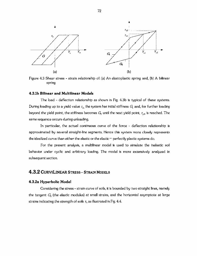
72
GA
(a) (b)
Figure 4.3 Shear stress - strain relationship of: (a) An elastoplastic spring and, (b) A bilinearspring
4.3.16 Bilinear and Multilinear Models
The load - deflection relationship as shown in Fig. 4.3b is typical of these systems.
During loading up to a yield value r, the system has initial stiffness G and, for further loading
beyond the yield point, the stiffness becomes 02 until the next yield point, re,, is reached. The
same sequence occurs during unloading.
In particular, the actual continuous curve of the force - deflection relationship is
approximated by several straight-line segments. Hence this system more closely represents
the idealized curve than either the elastic or the elastic - perfectly plastic systems do.
For the present analysis, a multilinear model is used to simulate the inelastic soil
behavior under cyclic and arbitrary loading. The model is more extensively analyzed in
subsequent section.
4.3.2 CURVILINEAR STRESS - STRAIN MODELS
4.3.2a Hyperbolic Model
Considering the stress - strain curve of soils, it is bounded by two straight lines, namely
the tangent Go (the elastic modulus) at small strains, and the horizontal asymptote at large
strains indicating the strength of soils r1, as illustrated in Fig. 4.4.
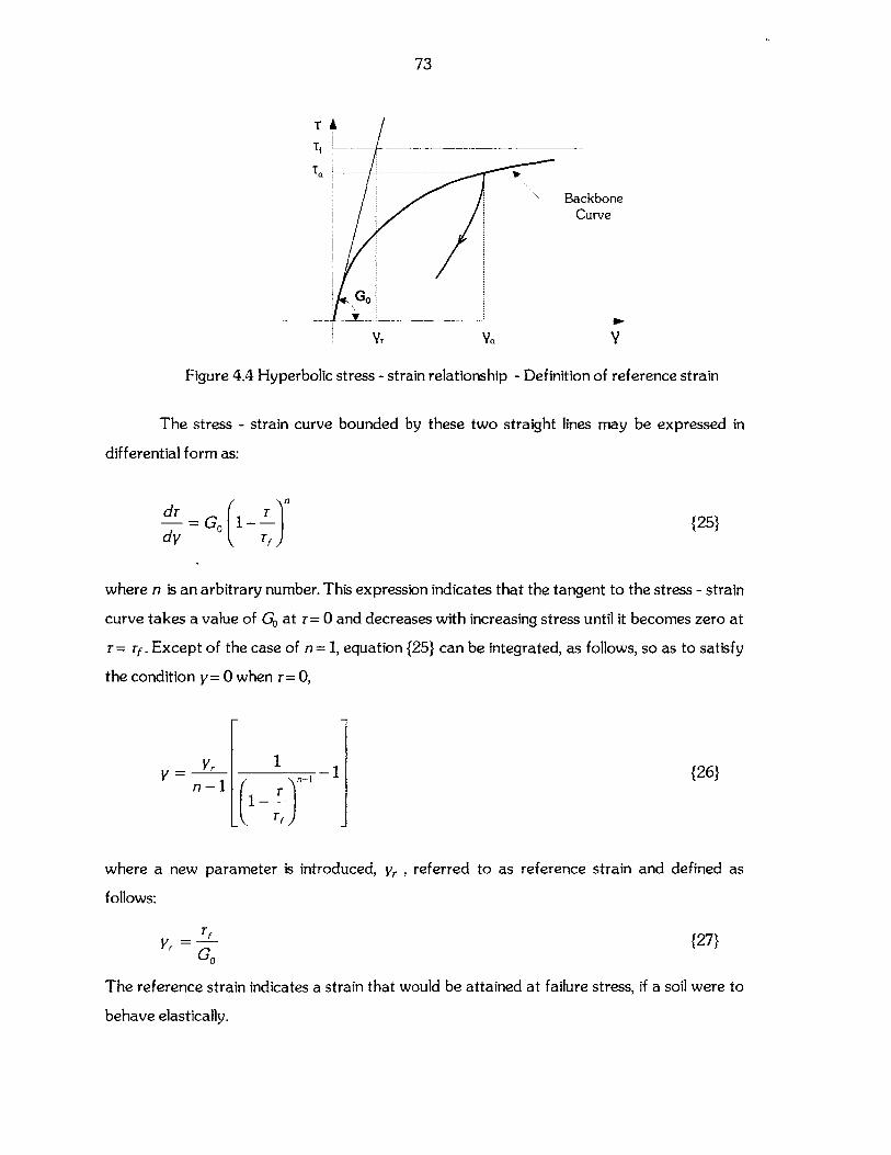
73
TALTf
Ta
BackboneCurve
y r yaQ y
Figure 4.4 Hyperbolic stress - strain relationship - Definition of reference strain
The stress - strain curve bounded by these two straight lines may be expressed in
dif ferential form as:
dT (1dT= G1
d y r,{25}
where n is an arbitrary number. This expression indicates that the tangent to the stress - strain
curve takes a value of Go at r= 0 and decreases with increasing stress until it becomes zero at
r= ry. Except of the case of n = 1, equation {25} can be integrated, as follows, so as to satisfy
the condition y=0 when r= 0,
{26}y = Yrn -1
where a new parameter is introduced, yr , referred to as reference strain and defined as
follows:
Vr TfY r {27}
The reference strain indicates a strain that would be attained at failure stress, if a soil were to
behave elastically.
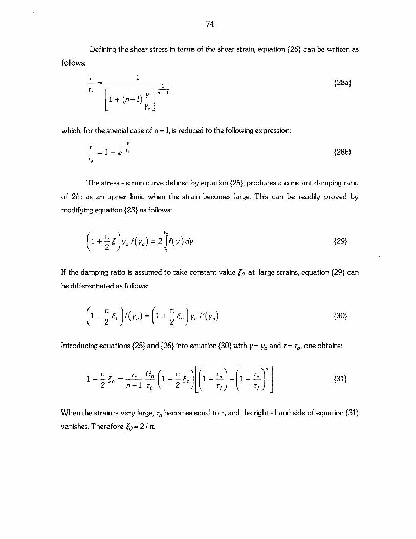
74
Defining the shear stress in terms of the shear strain, equation {26} can be written as
follows:
T- 1= {28a}
which, for the special case of n =1, is reduced to the following expression:
V
- = 1 - e v{28b)i-f
The stress - strain curve defined by equation {25}, produces a constant damping ratio
of 2/n as an upper limit, when the strain becomes large. This can be readily proved by
modifying equation {23} as follows:
1 2+JV I f(y0) = 2 ff(y) dy {29}0
If the damping ratio is assumed to take constant value lo at large strains, equation {29} can
be differentiated as follows:
21- f(y.)= V f'(yv) {30}
Introducing equations {25} and {26} into equation {30} with y= ya and r= ra, one obtains:
1- V G. 1 + n e 1 " - 1 " {31}1-2 eo n-1 ro 2 r, r,
When the strain is very large, T becomes equal to r, and the right - hand side of equation {31}
vanishes. Therefore o =2 / n.
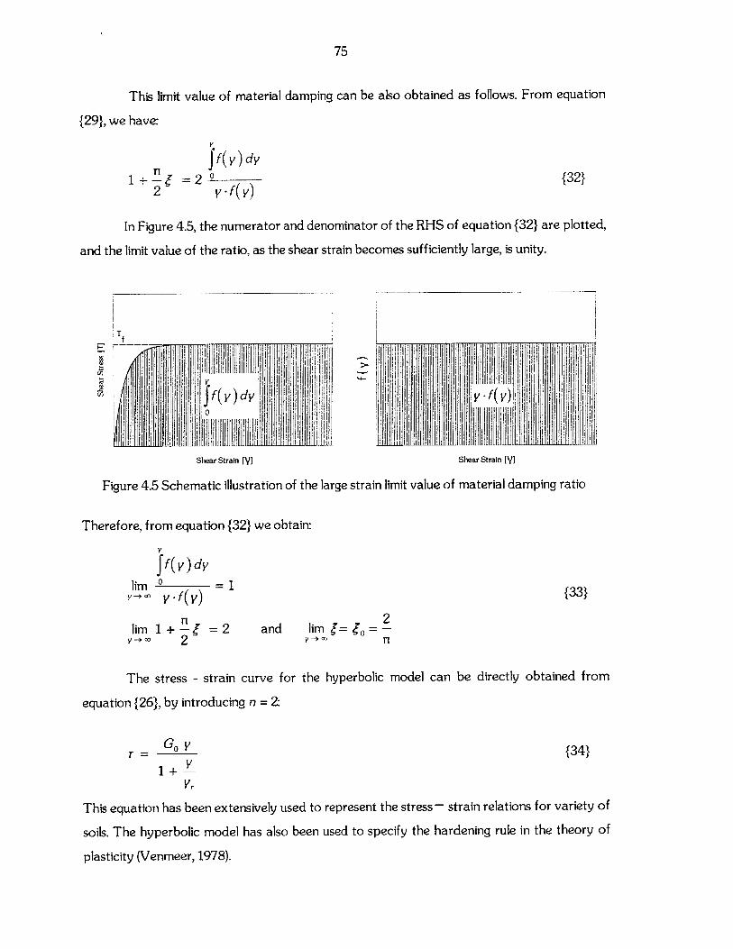
75
This limit value of material damping can be also obtained as follows. From equation
{29}, we have:
f(y) dy
1 + n =2 02 y-f(y)
{32}
In Figure 4.5,
and the limit value of
Tf
U)
aU)
the numerator and denominator of the RHS of equation {32} are plotted,
the ratio, as the shear strain becomes sufficiently large, is unity.
Shear Strain [y] Shear Strain [y]
Figure 4.5 Schematic illustration of the large strain limit value of material damping ratio
Therefore, from equation {32} we obtain:
ff(y)dy
lim =1Y--O y.f(y)
lim 1+ =2V -+ 00 2
{33}
2and liml=le=-
v -*C n
The stress - strain curve for the hyperbolic model can be directly obtained from
equation {26}, by introducing n = 2:
rT Go Y
1+Yr
{34}
This equation has been extensively used to represent the stress - strain relations for variety of
soils. The hyperbolic model has also been used to specify the hardening rule in the theory of
plasticity (Venmeer, 1978).
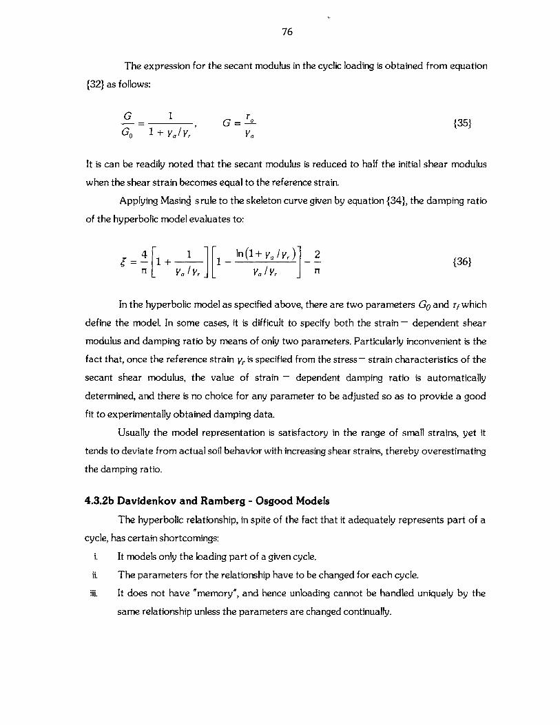
76
The expression for the secant modulus in the cyclic loading is obtained from equation
{32} as follows:
G _ 1 r 35-G-=, G =-"-{35}Go 1 + ya/ yr V,
It is can be readily noted that the secant modulus is reduced to half the initial shear modulus
when the shear strain becomes equal to the reference strain.
Applying Masing s rule to the skeleton curve given by equation {34}, the damping ratio
of the hyperbolic model evaluates to:
4 [1+ 1 1l_ In (1+ ya / Yr 1 {36}
n y" / yr ya / y, nl
In the hyperbolic model as specified above, there are two parameters Go and r, which
define the model. In some cases, it is difficult to specify both the strain - dependent shear
modulus and damping ratio by means of only two parameters. Particularly inconvenient is the
fact that, once the reference strain yr is specified from the stress- strain characteristics of the
secant shear modulus, the value of strain - dependent damping ratio is automatically
determined, and there is no choice for any parameter to be adjusted so as to provide a good
fit to experimentally obtained damping data.
Usually the model representation is satisfactory in the range of small strains, yet it
tends to deviate from actual soil behavior with increasing shear strains, thereby overestimating
the damping ratio.
4.3.2b Davidenkov and Ramberg - Osgood Models
The hyperbolic relationship, in spite of the fact that it adequately represents part of a
cycle, has certain shortcomings:
i. It models only the loading part of a given cycle.
ii. The parameters for the relationship have to be changed for each cycle.
iii. It does not have "memory", and hence unloading cannot be handled uniquely by the
same relationship unless the parameters are changed continually.
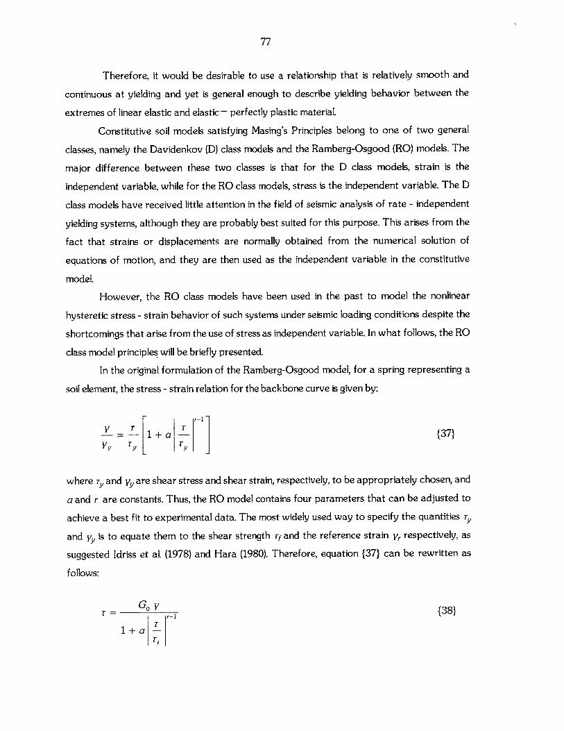
77
Therefore, it would be desirable to use a relationship that is relatively smooth and
continuous at yielding and yet is general enough to describe yielding behavior between the
extremes of linear elastic and elastic- perfectly plastic material.
Constitutive soil models satisfying Masing's Principles belong to one of two general
classes, namely the Davidenkov (D) class models and the Ramberg-Osgood (RO) models. The
major difference between these two classes is that for the D class models, strain is the
independent variable, while for the RO class models, stress is the independent variable. The D
class models have received little attention in the field of seismic analysis of rate - independent
yielding systems, although they are probably best suited for this purpose. This arises from the
fact that strains or displacements are normally obtained from the numerical solution of
equations of motion, and they are then used as the independent variable in the constitutive
model.
However, the RO class models have been used in the past to model the nonlinear
hysteretic stress - strain behavior of such systems under seismic loading conditions despite the
shortcomings that arise from the use of stress as independent variable. In what follows, the RO
class model principles will be briefly presented.
In the original formulation of the Ramberg-Osgood model, for a spring representing a
soil element, the stress - strain relation for the backbone curve is given by:
V- 1 +a T {37}
where ry and y are shear stress and shear strain, respectively, to be appropriately chosen, and
a and r are constants. Thus, the RO model contains four parameters that can be adjusted to
achieve a best fit to experimental data. The most widely used way to specify the quantities Ty
and Yy is to equate them to the shear strength Tf and the reference strain yr respectively, as
suggested Idriss et al. (1978) and Hara (1980). Therefore, equation {37} can be rewritten as
follows:
Go y {38}
1+ a T
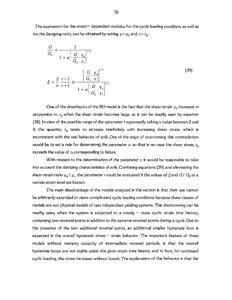
78
The expression for the strain- dependent modulus for the cyclic loading condition, as well as
for the damping ratio, can be obtained by setting y = ya and r= Ta:
G 1
Go G r-1G0 1+ a G "
Go y,
Gy' {39}
2 r-1 Go Y,
n r+1 G y1+a G "aGO Yr
One of the drawbacks of the RO model is the fact that the shear strain Va increases in
proportion to Ta when the shear strain becomes large, as it can be readily seen by equation
{38}. In view of the possible range of the parameter r supposedly taking a value between 2 and
4, the quantity Ta tends to increase indefinitely with increasing shear strain, which is
inconsistent with the real behavior of soils. One of the ways of overcoming this contradiction
would be to set a rule for determining the parameter a so that in no case the shear stress Ta
exceeds the value of Tf corresponding to failure.
With respect to the determination of the parameter r, it would be reasonable to take
into account the damping characteristics of soils. Combining equations {39} and eliminating the
shear strain ratio ya / y,, the parameter r could be evaluated if the values of eand G/ Go at a
certain strain level are known.
The main disadvantage of the models analyzed in this section is that their use cannot
be arbitrarily extended to more complicated cyclic loading conditions because these classes of
models are not physical models of rate independent yielding systems. This shortcoming can be
readily seen, when the system is subjected to a steady - state cyclic strain time history,
containing two reversal points in addition to the extreme reversal points during a cycle. Due to
the presence of the two additional reversal points, an additional smaller hysteresis loop is
expected in the overall hysteretic stress - strain behavior. The important feature of these
models without memory capacity of intermediate reversal periods, is that the overall
hysteresis loops are not stable under the given strain time history and in fact, for continued
cyclic loading, the stress increases without bound. The explanation of this behavior is that the
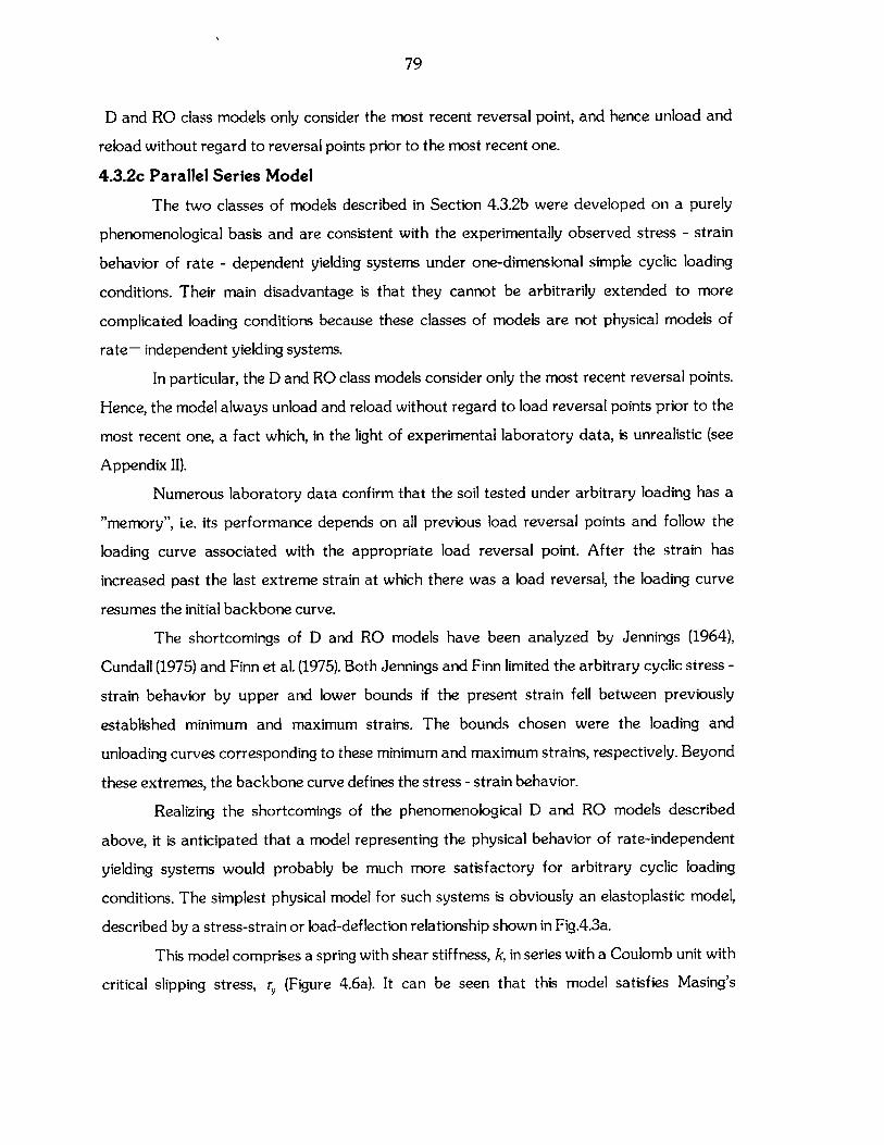
79
D and RO class models only consider the most recent reversal point, and hence unload and
reload without regard to reversal points prior to the most recent one.
4.3.2c Parallel Series Model
The two classes of models described in Section 4.3.2b were developed on a purely
phenomenological basis and are consistent with the experimentally observed stress - strain
behavior of rate - dependent yielding systems under one-dimensional simple cyclic loading
conditions. Their main disadvantage is that they cannot be arbitrarily extended to more
complicated loading conditions because these classes of models are not physical models of
rate- independent yielding systems.
In particular, the D and RO class models consider only the most recent reversal points.
Hence, the model always unload and reload without regard to load reversal points prior to the
most recent one, a fact which, in the light of experimental laboratory data, is unrealistic (see
Appendix II).
Numerous laboratory data confirm that the soil tested under arbitrary loading has a
"memory", i.e. its performance depends on all previous load reversal points and follow the
loading curve associated with the appropriate load reversal point. After the strain has
increased past the last extreme strain at which there was a load reversal, the loading curve
resumes the initial backbone curve.
The shortcomings of D and RO models have been analyzed by Jennings (1964),
Cundall (1975) and Finn et al. (1975). Both Jennings and Finn limited the arbitrary cyclic stress -
strain behavior by upper and lower bounds if the present strain fell between previously
established minimum and maximum strains. The bounds chosen were the loading and
unloading curves corresponding to these minimum and maximum strains, respectively. Beyond
these extremes, the backbone curve defines the stress - strain behavior.
Realizing the shortcomings of the phenomenological D and RO models described
above, it is anticipated that a model representing the physical behavior of rate-independent
yielding systems would probably be much more satisfactory for arbitrary cyclic loading
conditions. The simplest physical model for such systems is obviously an elastoplastic model,
described by a stress-strain or load-deflection relationship shown in Fig.4.3a.
This model comprises a spring with shear stiffness, k, in series with a Coulomb unit with
critical slipping stress, r (Figure 4.6a). It can be seen that this model satisfies Masing's
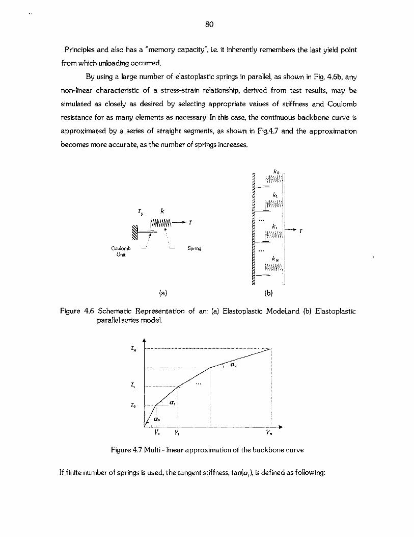
80
Principles and also has a "memory capacity", i.e. it inherently remembers the last yield point
from which unloading occurred.
By using a large number of elastoplastic springs in parallel, as shown in Fig. 4.6b, any
non-linear characteristic of a stress-strain relationship, derived from test results, may be
simulated as closely as desired by selecting appropriate values of stiffness and Coulomb
resistance for as many elements as necessary. In this case, the continuous backbone curve is
approximated by a series of straight segments, as shown in Fig.4.7 and the approximation
becomes more accurate, as the number of springs increases.
ko i
kk
TY kT ''k,-~ThT
Coulomb SpringUnit kN
kI
(a) (b)
Figure 4.6 Schematic Representation of an: (a) Elastoplasticparallel series model.
A
TN --------------- --------------- --------------
Modeland (b) Elastoplastic
KO V1 VN
Figure 4.7 Multi - linear approximation of the backbone curve
If finite number of springs is used, the tangent stiffness, tan(a, ), is defined as following:
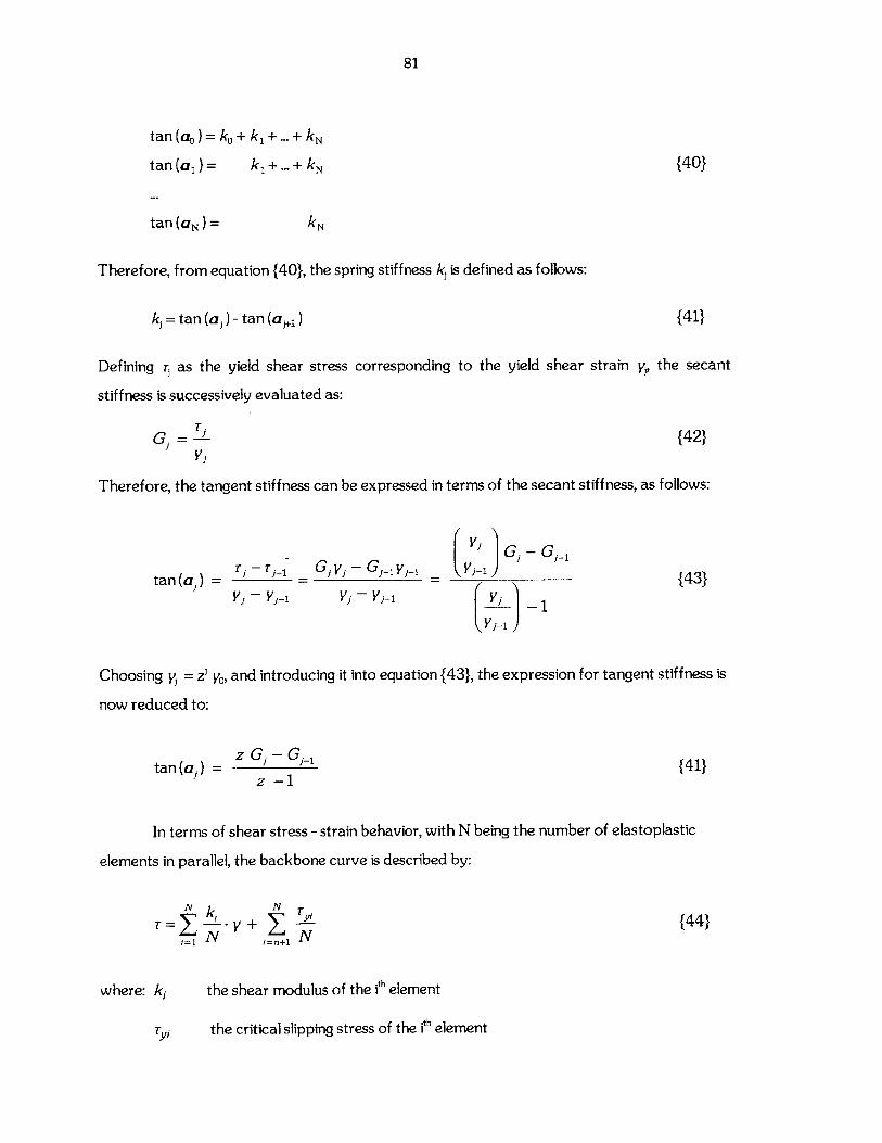
81
tan (ao )= ko + k1 + + kN
tan (a)= k+...+ kN {40}
tan (aN) kN
Therefore, from equation {40}, the spring stiffness kj is defined as follows:
kj= tan (a,)- tan (aj+) {41}
Defining , as the yield shear stress corresponding to the yield shear strain yj, the secant
stiffness is successively evaluated as:
T .Gj ={42}
V
Therefore, the tangent stiffness can be expressed in terms of the secant stiffness, as follows:
r, -Tjrl_. G, y, - Gj-j y,_ yjG -Gtan (a,) = 1 G 1 = J G- - {43}
Y, - Y,-1 V, - Y,-1 Y,
(V,-1
Choosing y, = zi yo, and introducing it into equation {43}, the expression for tangent stiffness is
now reduced to:
tan (a) = ' - {41}z -1
In terms of shear stress - strain behavior, with N being the number of elastoplastic
elements in parallel, the backbone curve is described by:
N N
r = -I - y1 + I i{44}j=1 N ,__n+ N
where: k, the shear modulus of the ith element
the critical slipping stress of the ith elementTy;
82
n the number of elements which remain elastic
r the shear stress on the backbone curve obtained for a given shear strain, y
Using the parallel series model described above for rate-independent yielding systems,
such as soils, the shear stress-strain relationship under arbitrary cyclic loading conditions can
be accurately represented, provided that it is updated with the appropriate reversal point
coordinates as the solution marches in time.
In what follows, the parallel series model shall be used for the performance of true
incremental non-linear analyses (see Chapters 5,6). For consistency, the shear stiffness of the
discrete elements is defined using stress - strain characteristics of the modified MIT-Si model
(see Chapter 3), and the material damping ratio is evaluated by integration of the shear stress-
strain hysteresis loop.
Consequently, results obtained by means of the nonlinear analysis are compared with
these obtained using the equivalent linear wave propagation analysis.
4.4 REFERENCES
Chen, W. F. & Mizuno, E. (1990). "Nonlinear Analysis in Soil Mechanics: Theory andImplementation', Developments in Geotechnical Engineering, Vol. 53, Elsevier SciencePublishers B.V.
Constantopoulos, I. V. (1973). 'Amplification Studies for a Nonlinear Hysteretic Soil Model',Research Report R73-46, Massachusetts Institute of Technology, September
Dames & Moore, Science Applications Inc. (1978). " Study of Nonlinear Effects on One -Dimensional Earthquake Response", prepared for Electric Power Research Institute,Projects 615-1,-2
Daniel, A. W. T., Harvey, R. C. and Burley, E. (1975). 'Stress - Strain Characteristics of Sand",Technical Note, Journal of the Geotechnical Division, ASCE, Vol.101, No. GT5, May, pp.508-512
Das, B. M. (1993). 'Principles of Soil Dynamics", PWS-KENT Publishing Company, Boston, MADobry, R. (1971). 'Soil Properties and the One-Dimensional Theory of Earthquake
Amplification", Research Report R71-18, Massachusetts Institute of TechnologyDrnevich, V. P., Hall, J. R. & Richard, F. E. Jr. (1967)." Effects of Amplitude of Vibration on the
Shear Modulus of Sand', Proc. International Symposium on Wave Propagation andDynamic Properties of Earth Materials, New Mexico, pp. 189-199
Finn, W. D. L., Lee, K. W. & Martin, G. R. (1975)." Stress-Strain Relations for Sand in SimpleSheaf , ASCE National Convention, Denver, Colorado, November, Meeting Reprint 2517
Hall, J. R. Jr. & Richard, F. E. Jr. (1963)." Dissipation of Elastic Wave Energy in GranularSoils" ,Journal of the Soil Mechanics and Foundation Division, ASCE, Vol. 98, No. SM6,November, pp. 27-56
83
Hardin, B.O. & Drnevich, V. P. (1972a)." Shear Modulus and Damping in Soils: I. Measurementand Parameter Effects' , Journal of the Soil Mechanics and Foundation Division, ASCE,Vol. 98, No. SM6, June, pp. 603-624
Hardin, B.O. & Drnevich, V. P. (1972b). " Shear Modulus and Damping in Soils: II. DesignEquations and Curveg' , Journal of the Soil Mechanics and Foundation Division, ASCE,Vol. 98, No. SM7, Juiy, pp. 667-692
Idriss, I. M., Dobry, R., Doyle, E. H. and Singh, R. D. (1976)." Behavior of Soft Clays underEarthquake Loading Conditions', Proc. Offshore Technology Conference, Paper No.OTC 2671, May
Ishihara, K. (1996). "Soil Behavior in Earthquake Geotechnics", Oxford Science Publications,Oxford Science Press, Walton Street, Oxford OX2 6DP
Iwan, W. D. (1967). " On a class of Models for the Yielding Behavior of Continuous andComposite Systems' , Journal of Applied Mechanics, Vol. 34, No. 3, September, pp. 612-617
Jennings, P. C. (1964). "Response of a General Yielding Structure". Journal of the EngineeringMechanics Division, ASCE, Vol. 90, EM2
Joyner, W. B. & Chen, A. T. F. (1975). " Calculation of Non-linear Ground Response inEarthquake' , Bulletin of the Seismological Society of America, Vol. 65, No. 5, October,pp. 1315-1336
Keydner, R. L.& Zelasko, J. S. (1963)." A Hyperbolic Stress - Strain Formulation for Sands' ,Proc. 2 d Pan American Conference on Soil Mechanics and Foundation Engineering,Vol. 1, Brazil
Konder, R. L. (1963)." Hyperbolic Stress-Strain Response: CohesiveSoils" ,Journal of the SoilMechanics and Foundation Division, ASCE, Vol. 89, No. SM1, February, pp.115-143
Krizek, R. J. & Franklin, A. G. (1968)." Energy Dissipation in a Soft Cla' , Proc. InternationalSymposium on Wave Propagation and Dynamic Properties of Earth Materials,University of New Mexico, pp. 797-807
Masing, G. (1926)." Eigenspannungen und Verfestigung beim Messing' , Proc. 2 "d InternationalCongress of Applied Mechanics, Zurich, pp. 332-335
Ramberg, W. & Osgood, W. R. (1943). " Description of Stress - Strain Curves by ThreeParameters" , Technical Note 902, NACA, July
Seed, H. B. & Idriss, I. M. (1970)." Soil Moduli and Damping Factors for Dynamic ResponseAnalyse"', Report No. EERC 70-10, Earthquake Engineering Research Center,University of California, Berkeley, December.
Shibuya, S., Mitachi, T. & Muira, S. (1994). "Pre-failure Deformation of Geomaterials", Proc.International Symposium on Pre-Failure Deformation Characteistics of Geomateria/s,Sapporo, Japan, September.
Silver, M. L. & Seed, H. B. (1971). " Deformation Characteristics of Sands under CyclicLoading , Journal of the Soil Mechanics and Foundations Division, ASCE, Vol. 97, No.SM8, August, pp. 1081-1098
Thiers, G. R. and Seed, H. B. (1968)." Cyclic Stress - Strain Characteristics of Clay' ,Journal ofthe Soil Mechanics and Foundation Division, ASCE, Vol. 60, No. 5, October, pp. 1625-1651
Weissman, G. F. & Hart, R. R. (1961). " The Damping Capacity of Some Granular Soilg',Symposium of Soil Dynamics, Special Technical Publication No. 305, American Societyfor Testing and Materials, pp. 15-19

84
Whitman, R. V. (1970). " Evaluation of Soil Properties for Site Evaluation and DynamicAnalysisof Nuclear Plants, Seismic Design for Nuclear Plants, R. J. Hanson (ed.), MITPress, Cambridge, Massachusetts
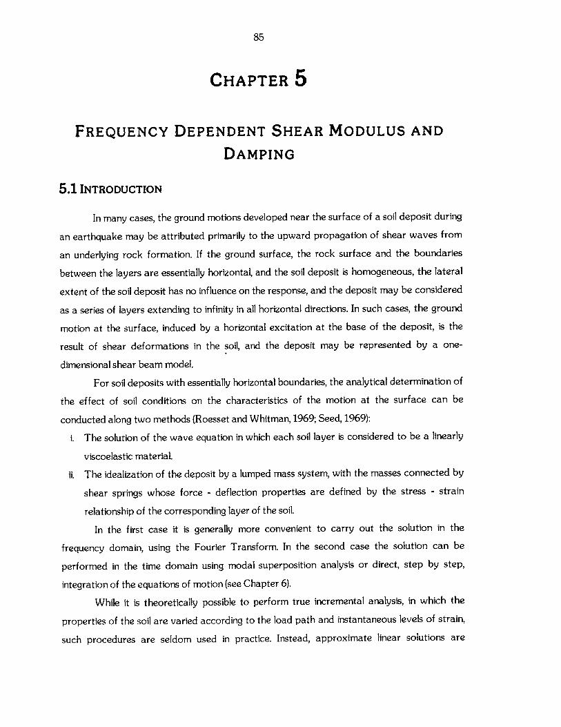
85
CHAPTER 5
FREQUENCY DEPENDENT SHEAR MODULUS AND
DAMPING
5.1 INTRODUCTION
In many cases, the ground motions developed near the surface of a soil deposit during
an earthquake may be attributed primarily to the upward propagation of shear waves from
an underlying rock formation. If the ground surface, the rock surface and the boundaries
between the layers are essentially horizontal, and the soil deposit is homogeneous, the lateral
extent of the soil deposit has no influence on the response, and the deposit may be considered
as a series of layers extending to infinity in all horizontal directions. In such cases, the ground
motion at the surface, induced by a horizontal excitation at the base of the deposit, is the
result of shear deformations in the soil, and the deposit may be represented by a one-
dimensional shear beam model.
For soil deposits with essentially horizontal boundaries, the analytical determination of
the effect of soil conditions on the characteristics of the motion at the surface can be
conducted along two methods (Roesset and Whitman, 1969; Seed, 1969):
i. The solution of the wave equation in which each soil layer is considered to be a linearly
viscoelastic material.
ii. The idealization of the deposit by a lumped mass system, with the masses connected by
shear springs whose force - deflection properties are defined by the stress - strain
relationship of the corresponding layer of the soil.
In the first case it is generally more convenient to carry out the solution in the
frequency domain, using the Fourier Transform. In the second case the solution can be
performed in the time domain using modal superposition analysis or direct, step by step,
integration of the equations of motion (see Chapter 6).
While it is theoretically possible to perform true incremental analysis, in which the
properties of the soil are varied according to the load path and instantaneous levels of strain,
such procedures are seldom used in practice. Instead, approximate linear solutions are
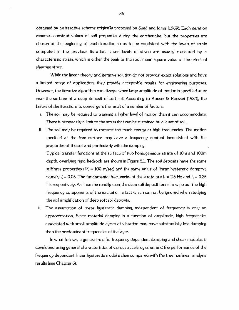
86
obtained by an iterative scheme originally proposed by Seed and Idriss (1969). Each iteration
assumes constant values of soil properties during the earthquake, but the properties are
chosen at the beginning of each iteration so as to be consistent with the levels of strain
computed in the previous iteration. These levels of strain are usually measured by a
characteristic strain, which is either the peak or the root mean square value of the principal
shearing strain.
While the linear theory and iterative solution do not provide exact solutions and have
a limited range of application, they provide acceptable results for engineering purposes.
However, the iterative algorithm can diverge when large amplitude of motion is specified at or
near the surface of a deep deposit of soft soil. According to Kausel & Roesset (1984), the
failure of the iterations to converge is the result of a number of factors:
i. The soil may be required to transmit a higher level of motion than it can accommodate.
There is necessarily a limit to the stress that can be sustained by a layer of soil.
ii. The soil may be required to transmit too much energy at high frequencies. The motion
specified at the free surface may have a frequency content inconsistent with the
properties of the soil and particularly with the damping.
Typical transfer functions at the surface of two homogeneous strata of 10m and 100m
depth, overlying rigid bedrock are shown in Figure 5.1. The soil deposits have the same
stiffness properties (V, = 100 m/sec) and the same value of linear hysteretic damping,
namely = 0.05. The fundamental frequencies of the strata are f, = 2.5 Hz and f, = 0.25
Hz respectively. As it can be readily seen, the deep soil deposit tends to wipe out the high
frequency components of the excitation, a fact which cannot be ignored when studying
the soil amplification of deep soft soil deposits.
iii. The assumption of linear hysteretic damping, independent of frequency is only an
approximation. Since material damping is a function of amplitude, high frequencies
associated with small amplitude cycles of vibration may have substantially less damping
than the predominant frequencies of the layer.
In what follows, a general rule for frequency dependent damping and shear modulus is
developed using general characteristics of various accelerograms, and the performance of the
frequency dependent linear hysteretic model is then compared with the true nonlinear analysis
results (see Chapter 6).
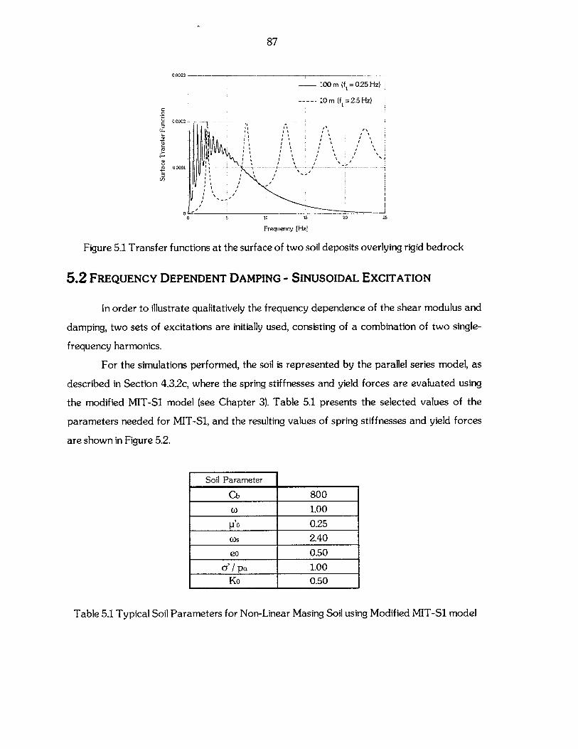
87
0.0003
m100 m (f = 025 Hz)
-O M (f 1=2.5Hz)0
.M 0.0002 - - -- -- -
0
( 0.0001- - --- ---- - / - - -
0 5 10 15 20 25
Frequency [Hzj
Figure 5.1 Transfer functions at the surface of two soil deposits overlying rigid bedrock
5.2 FREQUENCY DEPENDENT DAMPING - SINUSOIDAL EXCITATION
In order to illustrate qualitatively the frequency dependence of the shear modulus and
damping, two sets of excitations are initially used, consisting of a combination of two single-
frequency harmonics.
For the simulations performed, the soil is represented by the parallel series model, as
described in Section 4.3.2c, where the spring stiffnesses and yield forces are evaluated using
the modified MIT-Si model (see Chapter 3). Table 5.1 presents the selected values of the
parameters needed for MIT-Si, and the resulting values of spring stiffnesses and yield forces
are shown in Figure 5.2.
Soil Parameter
Cb 800
(a 1.00
p'o 0.25
Ws 2.40
eo 0.50o'I pa 1.00
Ko 0.50
Table 5.1 Typical Soil Parameters for Non-Linear Masing Soil using Modified MIT-Si model
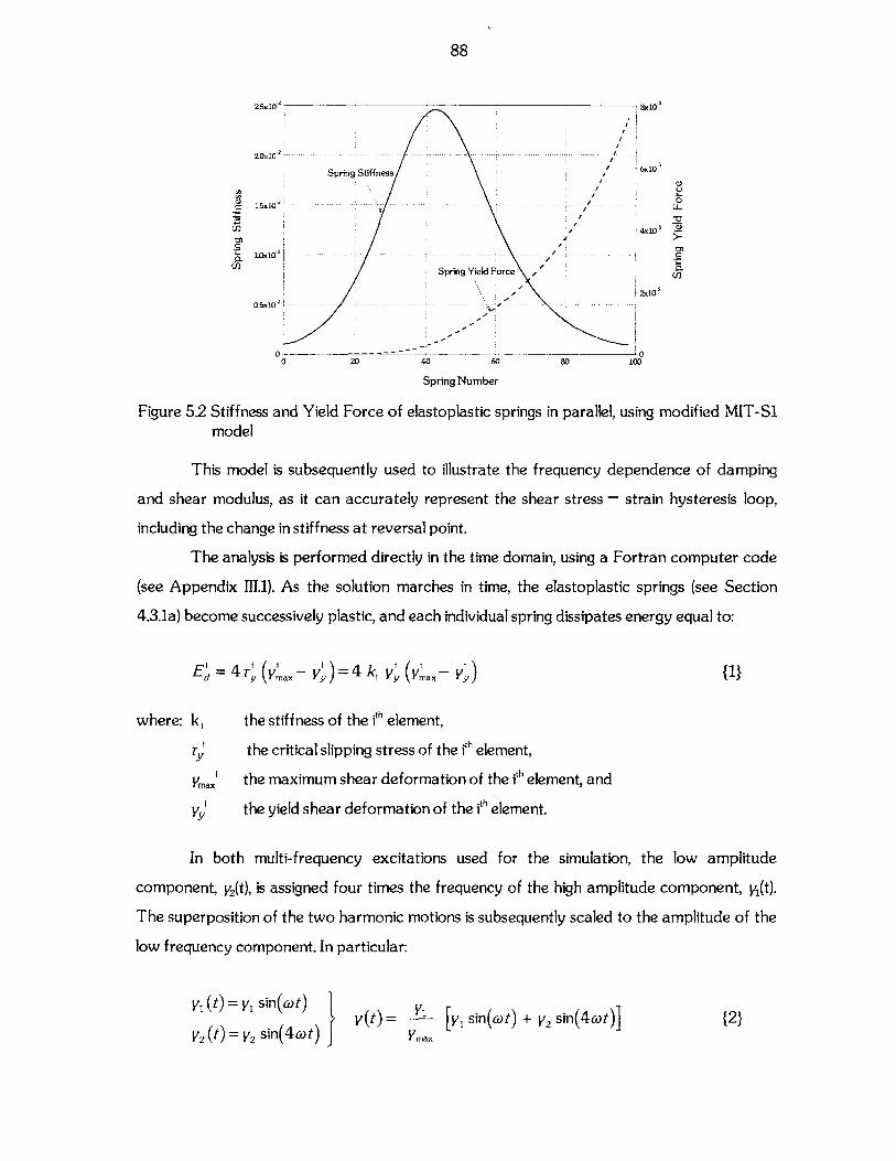
88
25x10- 8x10⁵
2-0 x 10 - - - - -- ----- - - ---- - --- - --
Z~6.10-'Spring Stiffness 6x10
4x10x0 2
L x10 - --- - --- -. - - - - - - -
Spring Yield Force
2x10s0.5x10 - - -- - - - -- - - -
0 0-- - -0 20 40 60 80 100
Spring Number
Figure 5.2 Stiffness and Yield Force of elastoplastic springs in parallel, using modified MIT-Simodel
This model is subsequently used to illustrate the frequency dependence of damping
and shear modulus, as it can accurately represent the shear stress - strain hysteresis loop,
including the change in stiffness at reversal point.
The analysis is performed directly in the time domain, using a Fortran computer code
(see Appendix 111.1). As the solution marches in time, the elastoplastic springs (see Section
4.3.1a) become successively plastic, and each individual spring dissipates energy equal to:
E = 4 ( ,x - vy = 4 k, y (y-ax y) {1}
where: k, the stiffness of the ith element,
T the critical slipping stress of the ith element,
ymax' the maximum shear deformation of the ith element, and
y the yield shear deformation of the ith element.
In both multi-frequency excitations used for the simulation, the low amplitude
component, y2(t), is assigned four times the frequency of the high amplitude component, y1(t).
The superposition of the two harmonic motions is subsequently scaled to the amplitude of the
low frequency component. In particular:
Y1 (t) = , sin(cot) } y(t)= V1 y, sin(Ct) + y2 sin(4ct)] {2}V2 (t) = y 2 sin(Amta) ymax
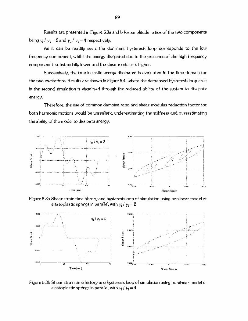
89
Results are presented in Figure 5.3a and b for amplitude ratios of the two components
being y / V2=2 and y1 / V2=4 respectively.
As it can be readily seen, the dominant hysteresis loop corresponds to the low
frequency component, whilst the energy dissipated due to the presence of the high frequency
component is substantially lower and the shear modulus is higher.
Successively, the true inelastic energy dissipated is evaluated in the time domain for
the two excitations. Results are shown in Figure 5.4, where the decreased hysteresis loop area
in the second simulation is visualized through the reduced ability of the system to dissipate
energy.
Therefore, the use of common damping ratio and shear modulus reduction factor for
both harmonic motions would be unrealistic, underestimating the stiffness and overestimating
the ability of the model to dissipate energy.
0.010 0.0015
Y1 / Y2= 2
aa
U)
/
Time [sec]
Shear strain time history and hysteresiselastoplastic springs in parallel, with y1 /
anU0
0-005
a5 5-0 7-0
Time [sec]
Figure 5.3b Shear strain time history and hysteresiselastoplastic springs in parallel, with y1 /
0.00005
-0.0005 L.....-0010
loop ofy2= 2
-0.005 0 0.005 0.010
Shear Strain
simulation using nonlinear model of
Q10000--
-0.0005
0.0005--- -- -- -- - - -- -
0010 0005 0 0.005 0010
Shear Strain
loop of simulation using nonlinear model of
y2= 4
In
0.005
-0.005
-0.010
.7
Figure 5.3a
0.010
0.005 /
a
aa-zU)
0.010 -
7 52 A so 0
1 /Y2=
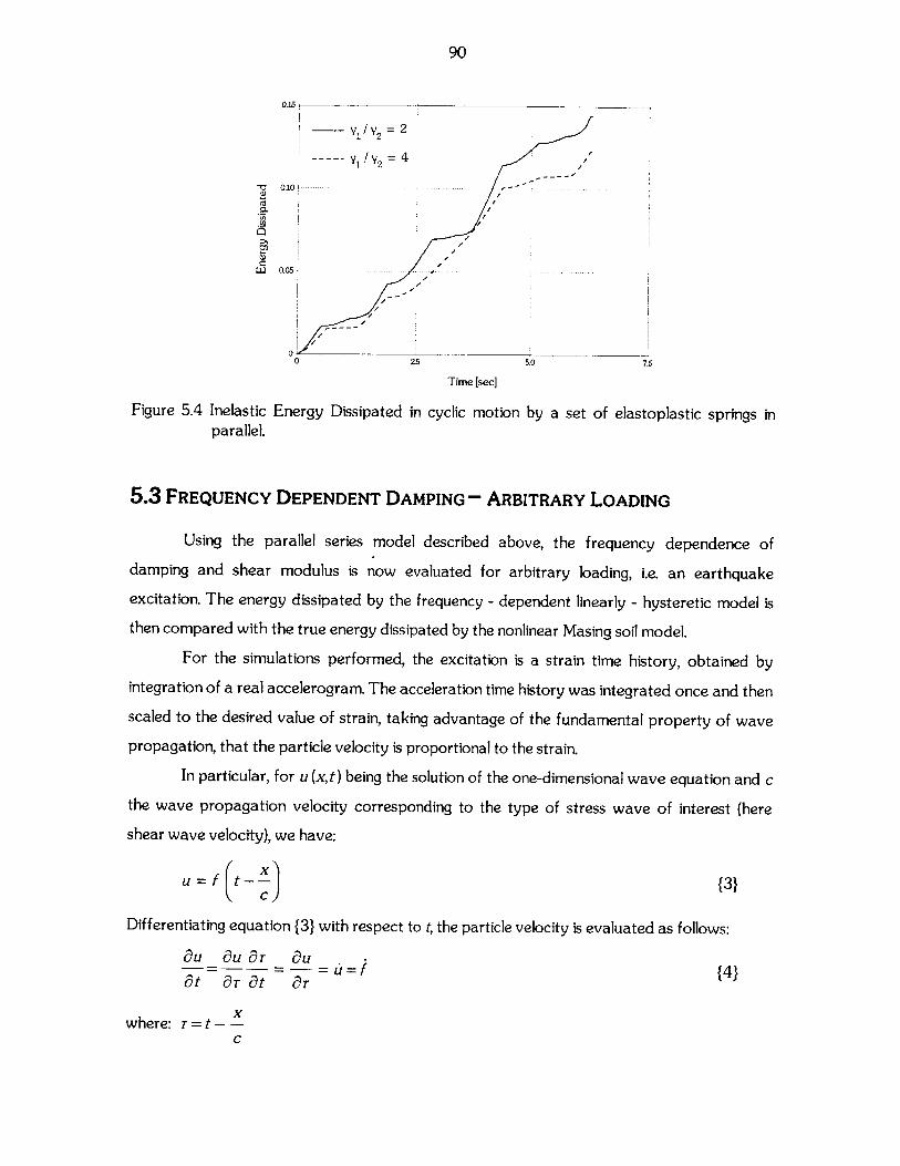
90
0.15
1 2---- ~ Y /y
15 2
"OC 0.10 - - --
LLJ 0.05
00 Z5 5.0 7.5
Time [sec]
Figure 5.4 Inelastic Energy Dissipated in cyclic motion by a set of elastoplastic springs inparallel.
5.3 FREQUENCY DEPENDENT DAMPING - ARBITRARY LOADING
Using the parallel series model described above, the frequency dependence of
damping and shear modulus is now evaluated for arbitrary loading, i.e. an earthquake
excitation. The energy dissipated by the frequency - dependent linearly - hysteretic model is
then compared with the true energy dissipated by the nonlinear Masing soil model.
For the simulations performed, the excitation is a strain time history, obtained by
integration of a real accelerogram. The acceleration time history was integrated once and then
scaled to the desired value of strain, taking advantage of the fundamental property of wave
propagation, that the particle velocity is proportional to the strain.
In particular, for u (xt) being the solution of the one-dimensional wave equation and c
the wave propagation velocity corresponding to the type of stress wave of interest (here
shear wave velocity), we have:
u = f t -j- {3}
Differentiating equation {3} with respect to t, the particle velocity is evaluated as follows:
au _U aT u- =- -= - ==f {4}t aT at ur
xwhere: T=t- -
C
91
Successively, differentiating equation {3} with respect to x, the shear strain is evaluated as
follows:
aU BU BrT 1 B3u_ 1y - auar - - - {5}
ax aax c ar c
Therefore, combining equations {4} and {5}, the shear strain (and shear stress) is proportional
to the particle velocity.
The distribution of the shear modulus reduction factor and damping in the frequency
domain, for the linear -hysteretic model, was evaluated by calculating the Fourier Transform
of the strain time history, scaling it to the maximum shear strain and successively assigning for
each discrete frequency values of modulus reduction and damping using the MIT-Si model
(see Chapter 3, equations {12} and {16}).
For consistency, the nonlinear springs of the Masing soil were evaluated using the same
soil model, with the characteristics described in Section 5.2.
5.3.1 ENERGY DISSIPATED - LINEAR HYSTERETIC MODEL
The energy dissipated for the frequency - dependent model was evaluated in the
frequency domain. In particular, the Fourier transform of the shear strain time history is
defined as:
y(t) = y(2)e'''tdw {6}
In analogy, the Fourier transform of the shear stress time history is:
r(t) = 21n fJ(co)e" do {7}
where: r(CO)= G [1+2 i (a) sgn(co)] y(w),
y (c) the Fourier transform of the shear strain time history, and
Z(o) the frequency dependent damping.
Therefore, the instantaneous power is given by the expression:
92
P(t) = T(t) '(t) = 12 f Tr(CO') y(O") i" e(("'+w")t dodor" {8}
Successively, the total energy dissipated by the linear - hysteretic model is evaluated as:
Ed= fP(t) dt =Jf 2 i j f r(o') y(")ico" e ddco dt {9}
Using the congruence 2in- e'c'' dt = 6 (O' +")
Ed = T(-O) y(co)jiw do2n
,the energy dissipated is:
{10}
Defining the complex conjugate r (-CO ) = r * (o)), and substituting in equation {10} the Fourier
transform of the shear stress from equation {7}, the energy dissipated is finally given by the
following equation':
Ed = fr'().y(co)i dco = -i[1-2il(w)sgn(co)] y'd =2 002 n d00
{11}G i 20 2G "0 (O O)I1d) 2 G 00S coJy dco + - cosgn(w){{w)|y|2 dc = G 0(() y|2de2 n 2n n _ymmetric
antisyrnmetric symrnetric
1 Note.-If damping was constant with frequency, the energy dissipated could be expressed directly in the timedomain. Using equation {7}, the shear stress is defined in the time domain as follows:
r(t)=G [y(t) + 2 4 P(t)]
where: f(t) = i sgn(o)] y(W) e''' dw is the Hilbert Transform of y(t).2 n -
Therefore, the power and the energy dissipated as a function of time would be evaluated as follows:
P(t) = T = G (y+2 P) y
Ed (t)= 2,rGj ydtd 0
93
With T being the duration of motion, the average power dissipated is defined as follows:
- Ed
T {12}
The RMS value of the shear strain, is obtained as an integral (summation) in the time
and frequency domain as following:
T
fy 2 dt -0
1 1T 2n
Jv2dko - {13}1 |y2 do,Tnf jdC
Considering that for a pure harmonic motion, the RMS value of the shear strain is
yp,,k = V yRms, we define:
k = %My s {14}
and therefore the maximum energy stored is evaluated as follows:
E= G Y2k = G y = |y|2 de {15}
From equations {11} and {15}, the equivalent energy ratio is defined as the following
integral ratio in the frequency domain:
1 Ed
4rn Es
10 n0n 0GJ) r~) Jyj2 d~o fO (co) Jy|2 dco
4 G 10* dy|12dco co f |y|2 dc
riT 0 ~c 0
where: coo = c=AT
2 1yus = T
{18}
94
5.3.2 ENERGY DISSIPATED - NONLINEAR PARALLEL SERIES MODEL
The energy dissipated for the nonlinear parallel series model was successively
evaluated directly in the time, as described in Section 5.2 for the sinusoidal loading. In
particular, using the notation introduced in 4.3.2c, the tangent and spring stiffnesses are
evaluated as follows:
_dr_
Gtan =d - G' y+Gdy
dG d2r""ta 2 Gry +2G'
dy dy
_(d2 dGtan
dyJ2 dy
Tangent Stiffness
{19}
Spring Stiffness
Therefore, the energy dissipated for an infinite number of elastoplastic springs is
evaluated as the integral (for the present analysis, finite number of springs was used):
Ymn
Ed= 4 fky(yma- y)dy0
=-4 f y (y - y)dyo V
4 ymaydGa" ydy - V'axdGtn V)2 dy0d 0 }
V. G dGtan V 2 1 -mx_2 f Gtn v dy
0
Y"'"x drT
Vmax dy0 dy
2 Gvdy -0
".a dr-2 y
0 dy
G y2
Ymax
-yG,,n Y1"+Yx y Gtan dy0
dy
After performing the algebraic operations and substituting from equation {19} the tangent and
secant moduli, the energy dissipated is calculated as:
=4
= 4
= 4
}
95
Ed= 4 2 Gydy -G y {20}f Vmax
Successively, the energy stored is evaluated as follows:
1E, = - G y2 {21}
2
Combining equations {20} and {21}, the hysteretic damping ratio, Z, is calculated as follows:
Vmax Vmax
1 Ed 2 2 GV 2 fd-- =-< 02 -1 >=-< -1 {22}4n E n Gy2 n 1 TsJmx[ -2 ymax J2
5.3.3 EXAMPLE OF APPLICATION
In what follows, the performance of the frequency-dependent linear-hysteretic model
is compared to the exact nonlinear solution, using the parallel series model. Both models were
coded in FORTRAN, and the computer code can be found in Appendix III.1. For the
simulation, the Kobe N-S accelerogram was used, the integral of which was scaled to V.ax =
0.001 and ymax = 0.05.
Results are shown in Figures 5.5 and 5.6 successively. For each simulation, the
following items are presented:
(a) the shear strain time history,
(b) the shear stress - strain hysteresis loop (nonlinear model),
(c), (d) the frequency dependent damping and shear modulus reduction factor, and
(e) comparison of the energy dissipated, evaluated using the two models.
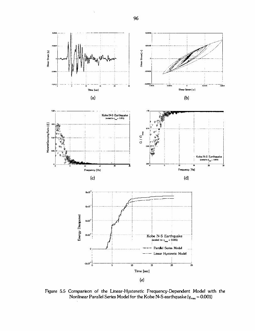
96
0-0010 0.00050
0-000s - - - - - - - -------- 0O00 5 - -- -.-
575- - - -- - -- - - -- 0000-
-0.000 s -- --- - -.. - . - .. - - -.... -.. . .......... o..o..... - ----- -- - -
0.0010 -0-900O0 0 10 is 20 25 -0.0000 -0.0005 0 00D005 0.000
Time [sec Shear Strain[ y]
(a) (b)
010 LOO~
Kobe NS Earthquake(scald t. 0.- -1-
D 0.10 -- .
On s -- ------- - - ------- - - - ---- - -- -- ---- - - -- -8x10xE
W 7 ~ ~ ~ 6 1 -- - -- S - --- ------_----- ---- - - ----- ------------ - - ..... .. .
~v V
Kobe N-S Earthquake(Lcaledto 001)
0 _ _ _ _ _ _ _ _ _ _ _ _ 025
0 5 10 150 20 25
Frequency (-Den Frequency [Hz]
(c) (d)
SX10-Kb7- Erhuk
6x......................... Paae ----es Model------------
Q(e
NonlnearParalel erie Modl-fo-theKob N-S Earthquake ----- 0.001
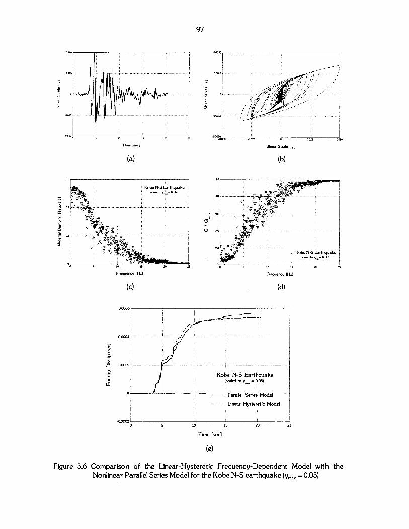
U,
Kobe N-S Earthquake(Scaldtoy =005)
E
--- -- -- ---- ---- --- ---- -- --- - ---- -- ---- ---- -- -- -- ---- -- --- ---- --- -- ----
Kobe N-S Earthqi(scaled to y = 0.05
Paralel SeriesT - TILM
15
Time [sec]
(e)
Figure 5.6 Comparison of the Linear-Hysteretic Frequency-Dependent Model with theNonlinear Parallel Series Model for the Kobe N-S earthquake (ymax = 0.05)
97
U,
U,
Time [sec]
(a)
Shear Strain [ y]
(b)
Z
0
10 15
Frequency [Hz]
(c)
0.0006
Frequency [Hz]
(d)
0.0004
0)
0)0)Cw
0.0002
0
uake
lodel
0 5 10 20 25
all
near ysteretic Model
98
As it can be readily seen, results of the frequency dependent linear hysteretic model
are in very good agreement with the nonlinear parallel series model. As it was expected, the
distribution of shear modulus reduction factor and damping in the frequency domain shows
that the model has a stiffer response and therefore dissipates less energy due to the high
frequency components of the excitation.
In what follows, a general rule for the distribution of strain in the frequency domain is
developed. By this approximation, an attempt to avoid errors arising from numerical
instabilities due to the spikes characterizing the exact Fourier transform, and on the same time
to accelerate the time required for the solution of the wave propagation problem, using the
linear-hysteretic, frequency-dependent damping model, is made.
5.4 SMOOTHED STRAIN DISTRIBUTION IN THE FREQUENCY DOMAIN
In order to develop a general rule for the distribution of strain in the frequency domain,
various accelerograms were used, namely Helena, Golden Gate, Kobe, Pacoima Dam, Loma
Prieta, Olympia, San Fernando, Parkfield and El Centro.
The strain time history was successively approximated, by integrating the acceleration
time histories once, and scaling them to the desired maximum strain value, according to the
rationale described in Section 5.3.
Figure 5.7 shows the Fourier transform of the strain time histories obtained as
described above and successively scaled to the same mean value in the frequency range 0 - 5
Hz. As it can be readily seen, the distribution of the strain in the frequency domain for all the
earthquakes under consideration was approximately the same and therefore, a smoothed
curve could approximate within desired degree of accuracy, the exact distribution.
The smoothed curve to fit the strain distribution in the frequency domain was chosen
to be the following:
exp(-0.15.f)y = yo - 0.62s 23
(f +1)
where: yo maximum strain amplitude, and
f frequency [Hz].
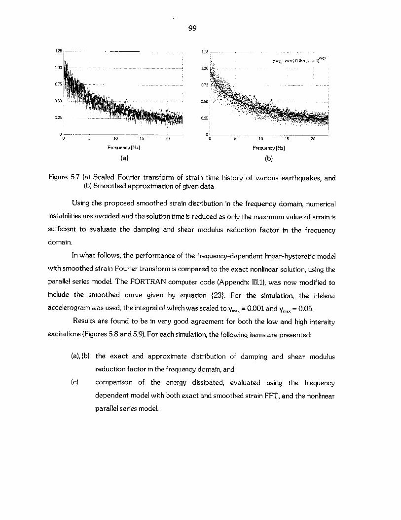
99
1.25
= exp (-0.15 x ) / (x+1)
0.75 ------ --- 0.75 -j '
0.50 - - ----. 50
0.25 -- ----- - - --- 0.25 -
0 00 5 10 15 20 0 5 10 15 20
Frequency [Hz] Frequency [Hz]
(a) (b)
Figure 5.7 (a) Scaled Fourier transform of strain time history of various earthquakes, and(b) Smoothed approximation of given data
Using the proposed smoothed strain distribution in the frequency domain, numerical
instabilities are avoided and the solution time is reduced as only the maximum value of strain is
sufficient to evaluate the damping and shear modulus reduction factor in the frequency
domain.
In what follows, the performance of the frequency-dependent linear-hysteretic model
with smoothed strain Fourier transform is compared to the exact nonlinear solution, using the
parallel series model. The FORTRAN computer code (Appendix 111.1), was now modified to
include the smoothed curve given by equation {23}. For the simulation, the Helena
accelerogram was used, the integral of which was scaled to ymax = 0.001 and yVax = 0.05.
Results are found to be in very good agreement for both the low and high intensity
excitations (Figures 5.8 and 5.9). For each simulation, the following items are presented:
(a), (b) the exact and approximate distribution of damping and shear modulus
reduction factor in the frequency domain, and
(c) comparison of the energy dissipated, evaluated using the frequency
dependent model with both exact and smoothed strain FFT, and the nonlinear
parallel series model.
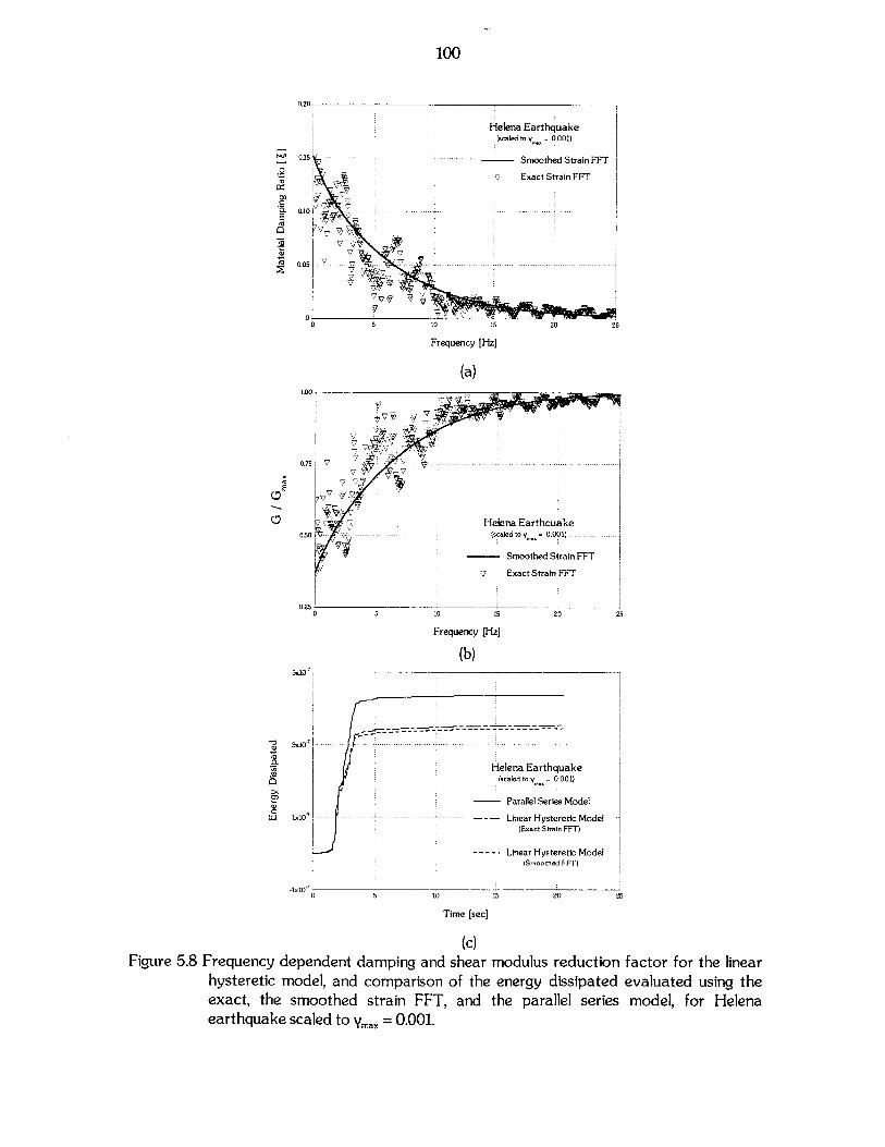
100
Helena Earthquake(scaled to y = 0.001)
Smoothed Strain FFT
Exact Strain FFT
0.05
Frequency [Hz]
(a)
Frequency [Hz]
(b)
5 10 15 20 25
Time [sec]
(c)Figure 5.8 Frequency dependent damping and shear modulus reduction factor for the linear
hysteretic model, and comparison of the energy dissipated evaluated using theexact, the smoothed strain FFT, and the parallel series model, for Helenaearthquake scaled to ymax = 0.001.
.2CO
0,
Ea
0)a
E
5x10'
3x10~0aa0.
0,
Lu
0
-- ----- - --- - ----- - - -
Helena Earthqu(scaled to y 0.0
Parallel Series
-- -.- Linear Hyste(Exact Strain FT
-Linear Hyster M(Smoothed
ake01)
Model
etic Model
etic ModelFFT)
wx104
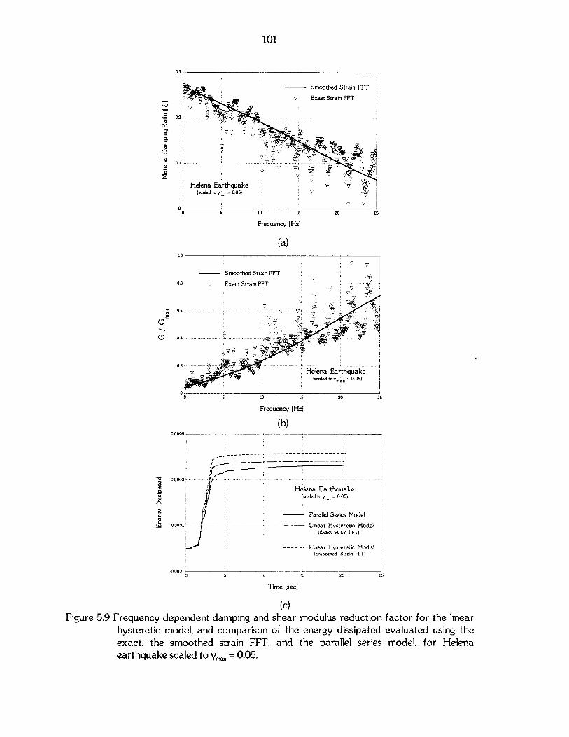
101
Smoothed Strain FFT
7 Exast Strain FFT
7'
Helena E(scaled to y
arthquake-7
=0.05) 1
5 10 15 20 25
Frequency [Hz]
(a)1O
X
0E
0 5 10 15
Frequency [Hz]
20 25
(b)
----------------- - - - -
Helena Earthquake(scaled to y 0.05)
Parallel Series Model
--- --- - -. -. - - Linear Hysteretic Model(Exact Strain FFT)
--- - - ----- Linear Hysteretic Model(Smoothed Strain FFT)
0000110 5 10 15 20 25
Time [sec]
(c)Figure 5.9 Frequency dependent damping and shear modulus reduction factor for the linear
hysteretic model, and comparison of the energy dissipated evaluated using theexact, the smoothed strain FFT, and the parallel series model, for Helenaearthquake scaled to ymax = 0.05.
0
E
02
0.1
00
0.0005
-oa(0
Li-I
0.0003
0.0001
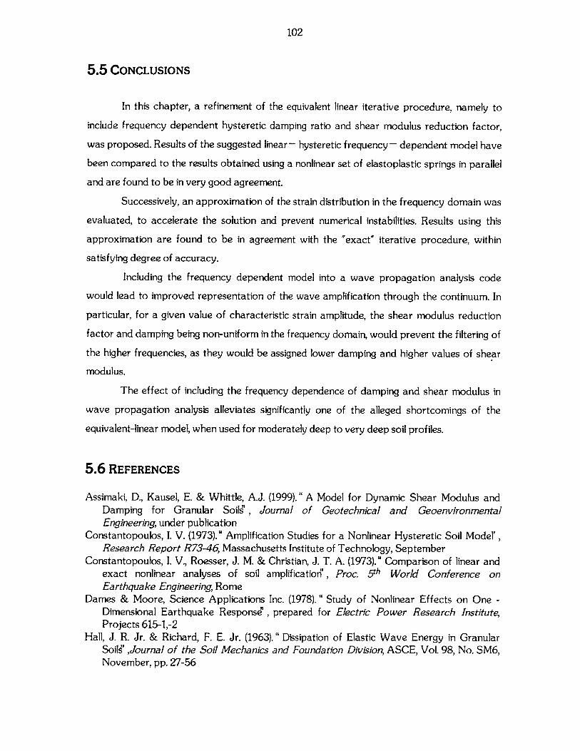
102
5.5 CONCLUSIONS
In this chapter, a refinement of the equivalent linear iterative procedure, namely to
include frequency dependent hysteretic damping ratio and shear modulus reduction factor,
was proposed. Results of the suggested linear - hysteretic frequency - dependent model have
been compared to the results obtained using a nonlinear set of elastoplastic springs in parallel
and are found to be in very good agreement.
Successively, an approximation of the strain distribution in the frequency domain was
evaluated, to accelerate the solution and prevent numerical instabilities. Results using this
approximation are found to be in agreement with the 'exact" iterative procedure, within
satisfying degree of accuracy.
Including the frequency dependent model into a wave propagation analysis code
would lead to improved representation of the wave amplification through the continuum. In
particular, for a given value of characteristic strain amplitude, the shear modulus reduction
factor and damping being non-uniform in the frequency domain, would prevent the filtering of
the higher frequencies, as they would be assigned lower damping and higher values of shear
modulus.
The effect of including the frequency dependence of damping and shear modulus in
wave propagation analysis alleviates significantly one of the alleged shortcomings of the
equivalent-linear model, when used for moderately deep to very deep soil profiles.
5.6 REFERENCES
Assimaki, D., Kausel, E. & Whittle, A.J. (1999)." A Model for Dynamic Shear Modulus andDamping for Granular Soil?', Journal of Geotechnical and GeoenvironmentalEngineering, under publication
Constantopoulos, I. V. (1973)." Amplification Studies for a Nonlinear Hysteretic Soil Model',Research Report R73-46, Massachusetts Institute of Technology, September
Constantopoulos, I. V., Roesser, J. M. & Christian, J. T. A. (1973)." Comparison of linear andexact nonlinear analyses of soil amplification , Proc. 5 th World Conference onEarthquake Engineering, Rome
Dames & Moore, Science Applications Inc. (1978)." Study of Nonlinear Effects on One -Dimensional Earthquake Response", prepared for Electric Power Research Institute,Projects 615-1,-2
Hall, J. R. Jr. & Richard, F. E. Jr. (1963). " Dissipation of Elastic Wave Energy in GranularSoils' ,Journal of the Soil Mechanics and Foundation Division, ASCE, Vol. 98, No. SM6,November, pp. 27-56
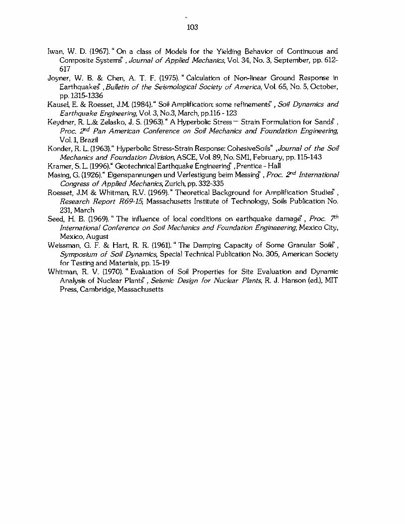
103
Iwan, W. D. (1967). " On a class of Models for the Yielding Behavior of Continuous andComposite Systems , Journal of Applied Mechanics, Vol. 34, No. 3, September, pp. 612-617
Joyner, W. B. & Chen, A. T. F. (1975). " Calculation of Non-linear Ground Response inEarthquakes , Bulletin of the Seismological Society of America, Vol. 65, No. 5, October,pp. 1315-1336
Kausel, E. & Roesset, J.M. (1984)." Soil Amplification: some refinements , Soil Dynamics and
Earthquake Engineering, Vol. 3, No.3, March, pp.1 1 6 - 123Keydner, R. L.& Zelasko, J. S. (1963)." A Hyperbolic Stress - Strain Formulation for Sands ,
Proc. 2 d Pan American Conference on Soil Mechanics and Foundation Engineering,Vol. 1, Brazil
Konder, R. L. (1963)." Hyperbolic Stress-Strain Response: CohesiveSoils" ,Journal of the Soil
Mechanics and Foundation Division, ASCE, Vol. 89, No. SM1, February, pp. 115-143Kramer, S. L. (1996)." Geotechnical Earthquake Engineerin ' , Prentice - HallMasing, G. (1926)." Eigenspannungen und Verfestigung beim Messing' , Proc. 2 d International
Congress of Applied Mechanics, Zurich, pp. 332-335Roesset, J.M & Whitman, R.V. (1969)." Theoretical Background for Amplification Studies ,
Research Report R69-15, Massachusetts Institute of Technology, Soils Publication No.231, March
Seed, H. B. (1969). " The influence of local conditions on earthquake damage , Proc. 7th
International Conference on Soil Mechanics and Foundation Engineeering, Mexico City,Mexico, August
Weissman, G. F. & Hart, R. R. (1961). " The Damping Capacity of Some Granular Soilg',Symposium of Soil Dynamics, Special Technical Publication No. 305, American Societyfor Testing and Materials, pp. 15-19
Whitman, R. V. (1970). " Evaluation of Soil Properties for Site Evaluation and DynamicAnalysis of Nuclear Plants , Seismic Design for Nuclear Plants, R. J. Hanson (ed.), MIT
Press, Cambridge, Massachusetts

104
105
CHAPTER 6
COMPARISON OF LINEAR AND EXACT NONLINEAR
ANALYSIS OF SOIL AMPLIFICATION
6.1 INTRODUCTION
In the previous chapters of the present study, two major disadvantages of the equivalent
linear iterative algorithm for soil amplification of deep deposits were studied in detail. In particular:
i. The shear modulus degradation and damping curves originally proposed by Seed & Idriss,
1969, and widely used in practice, are essentially the same for sands, gravels and
cohesionless silts, and are independent of the cycle number considered, as well as the void
ratio (or relative density), sand type and confining pressure. Laboratory experimental data
provide evidence in support of some of the above simplifications, yet prove that the
influence of confining pressure is significant and cannot be ignored, especially when dynamic
analyses for deep soil deposits are performed.
ii. The assumption of a linear hysteretic damping, independent of frequency is only an
approximation, which leads to non-realistic results when wave propagation in deep soil
deposits is studied. As a result of this simplification, the high frequency components of
the base excitation are artificially suppressed by the uniform distribution of hysteretic
damping in the frequency domain.
Attempting to overcome the aforementioned shortcomings, two refinements to the
linear iterative algorithm were introduced, namely:
i. A theoretical four - parameter soil model, derived from MIT-S1, with analytical
expressions for the shear modulus reduction factor and damping versus shear strain
amplitude, which depend on the soil type and the soil current state (void ratio and mean
effective stress) and nonlinear characteristics (small strain nonlinearity).
ii. A frequency - dependent linear - hysteretic model, with analytical expressions for the
shear modulus reduction factor and damping in the frequency domain.
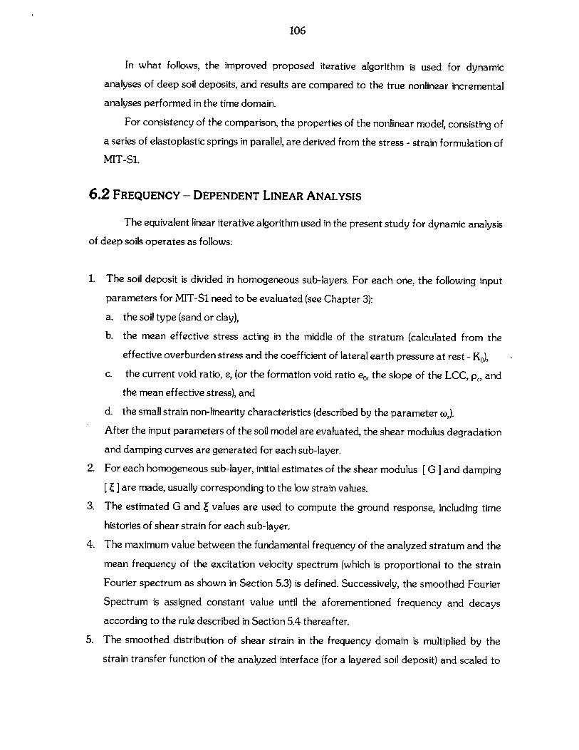
106
In what follows, the improved proposed iterative algorithm is used for dynamic
analyses of deep soil deposits, and results are compared to the true nonlinear incremental
analyses performed in the time domain.
For consistency of the comparison, the properties of the nonlinear model, consisting of
a series of elastoplastic springs in parallel, are derived from the stress - strain formulation of
MIT-S1.
6.2 FREQUENCY - DEPENDENT LINEAR ANALYSIS
The equivalent linear iterative algorithm used in the present study for dynamic analysis
of deep soils operates as follows:
1. The soil deposit is divided in homogeneous sub-layers. For each one, the following input
parameters for MIT-Sl need to be evaluated (see Chapter 3):
a. the soil type (sand or clay),
b. the mean effective stress acting in the middle of the stratum (calculated from the
effective overburden stress and the coefficient of lateral earth pressure at rest - KO),
c. the current void ratio, e, (or the formation void ratio eo, the slope of the LCC, pc, and
the mean effective stress), and
d. the small strain non-linearity characteristics (described by the parameter oz).
After the input parameters of the soil model are evaluated, the shear modulus degradation
and damping curves are generated for each sub-layer.
2. For each homogeneous sub-layer, initial estimates of the shear modulus [ G ] and damping
[( ] are made, usually corresponding to the low strain values.
3. The estimated G and Z values are used to compute the ground response, including time
histories of shear strain for each sub-layer.
4. The maximum value between the fundamental frequency of the analyzed stratum and the
mean frequency of the excitation velocity spectrum (which is proportional to the strain
Fourier spectrum as shown in Section 5.3) is defined. Successively, the smoothed Fourier
Spectrum is assigned constant value until the aforementioned frequency and decays
according to the rule described in Section 5.4 thereafter.
5. The smoothed distribution of shear strain in the frequency domain is multiplied by the
strain transfer function of the analyzed interface (for a layered soil deposit) and scaled to
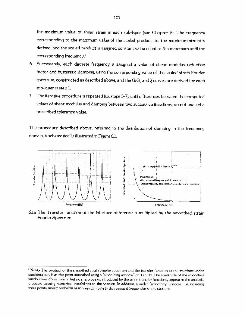
107
the maximum value of shear strain in each sub-layer (see Chapter 5). The frequency
corresponding to the maximum value of the scaled product (i.e. the maximum strain) is
defined, and the scaled product is assigned constant value equal to the maximum until the
corresponding frequency.'
6. Successively, each discrete frequency is assigned a value of shear modulus reduction
factor and hysteretic damping, using the corresponding value of the scaled strain Fourier
spectrum, constructed as described above, and the G/Go and Z curves are derived for each
sub-layer in step 1.
7. The iterative procedure is repeated (i.e. steps 5-7), until differences between the computed
values of shear modulus and damping between two successive iterations, do not exceed a
prescribed tolerance value.
The procedure described above, referring to the distribution of damping in the frequency
domain, is schematically illustrated in Figure 6.1.
00
Maximum of-I -Fundamental Frequency of Stratum, or
- -- -- -- -rFreuny of Excitation Foier Spectrum
Frequency [Hz] Frequency [Hz]
6.1a The Transfer function of the interface of interest is multiplied by the smoothed strainFourier Spectrum
Note.- The product of the smoothed strain Fourier spectrum and the transfer function at the interface underconsideration, is at this point smoothed using a "smoothing window' of 0.75 Hz. The amplitude of the smoothedwindow was chosen such that no sharp peaks, introduced by the strain transfer functions, appear in the analysis,probably causing numerical instabilities to the solution. In addition, a wider "smoothing window", i.e. includingmore points, would probably assign less damping to the resonant frequencies of the stratum.
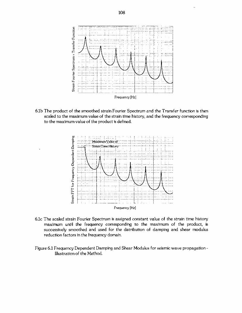
108
U
fni
E
Frequency [Hz]
6.1b The product of the smoothed strain Fourier Spectrum and the Transfer function is thenscaled to the maximum value of the strain time history, and the frequency correspondingto the maximum value of the product is defined.
E Maximum Value-
Strain Time 'History I
maiumutl th2rqec orsodn otemxmmo h rdci
successively smote and used for t dr i o a n ns r ur- ft in th frequency domain.F) 6.1 Frequency D e n a ia Sa o ufsm w e p tn
Is t of the Method... - ----....
-0-)- --- -- -- - -- -
--------)- --
--H- --- -- ---- -- -7- ----.. -------- ----- ---- -- - -- - - --- --- - ---
7 - - --- -- --- ---
----__ _ _----
---- Frequency- [Hz
reduction~~Frqunc fatr[iHhzreuny]oan
Figure 6.1 Frequency Dependent Damping and Shear Modulus for seismic wave propagation -Illustration of the Method.
--- - ------
---------- ------------------ -
----------- ---
- --- ---- --
. . .......... -
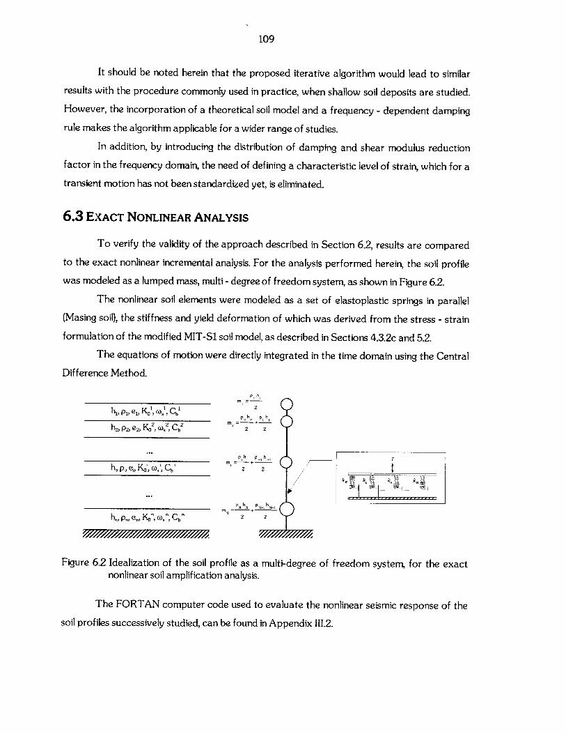
109
It should be noted herein that the proposed iterative algorithm would lead to similar
results with the procedure commonly used in practice, when shallow soil deposits are studied.
However, the incorporation of a theoretical soil model and a frequency - dependent damping
rule makes the algorithm applicable for a wider range of studies.
In addition, by introducing the distribution of damping and shear modulus reduction
factor in the frequency domain, the need of defining a characteristic level of strain, which for a
transient motion has not been standardized yet, is eliminated.
6.3 EXACT NONLINEAR ANALYSIS
To verify the validity of the approach described in Section 6.2, results are compared
to the exact nonlinear incremental analysis. For the analysis performed herein, the soil profile
was modeled as a lumped mass, multi - degree of freedom system, as shown in Figure 6.2.
The nonlinear soil elements were modeled as a set of elastoplastic springs in parallel
(Masing soil), the stiffness and yield deformation of which was derived from the stress - strain
formulation of the modified MIT-Si soil model, as described in Sections 4.3.2c and 5.2.
The equations of motion were directly integrated in the time domain using the Central
Difference Method.
p Ih
2
hi, pi, el, Kol , C h 2 1hp2h2 ih
h2, P2, e 2, K02 , f, C. 2 2 2
h, p,, e, K", (o", "b 2 2
__________________________p,_ ph, p, h.
hn, pn, en, Ko, )' n' C. 2 2
Figure 6.2 Idealization of the soil profile as a multi-degree of freedom system, for the exactnonlinear soil amplification analysis.
The FORTAN computer code used to evaluate the nonlinear seismic response of the
soil profiles successively studied, can be found in Appendix 111.2.
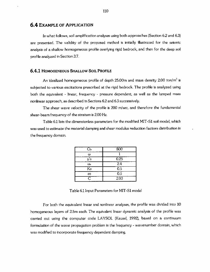
110
6.4 EXAMPLE OF APPLICATION
In what follows, soil amplification analyses using both approaches (Section 6.2 and 6.3)
are presented. The validity of the proposed method is initially illustrated for the seismic
analysis of a shallow homogeneous profile overlying rigid bedrock, and then for the deep soil
profile analyzed in Section 3.7.
6.4.1 HOMOGENEOUS SHALLOW SOIL PROFILE
An idealized homogeneous profile of depth 25.00m and mass density 2.00 ton/m3 is
subjected to various excitations prescribed at the rigid bedrock. The profile is analyzed using
both the equivalent - linear, frequency - pressure dependent, as well as the lumped mass
nonlinear approach, as described in Sections 6.2 and 6.3 successively.
The shear wave velocity of the profile is 200 m/sec, and therefore the fundamental
shear-beam frequency of the stratum is 2.00 Hz.
Table 6.1 lists the dimensionless parameters for the modified MIT-Si soil model, which
was used to estimate the material damping and shear modulus reduction factors distribution in
the frequency domain.
Cb 8000) 1
p'o 0.25Cos 2.4Ko 0.5eo 0.5C 2.03
Table 6.1 Input Parameters for MIT-Si model
For both the equivalent linear and nonlinear analyses, the profile was divided into 10
homogeneous layers of 2.5m each. The equivalent linear dynamic analysis of the profile was
carried out using the computer code LAYSOL (Kausel, 1992), based on a continuum
formulation of the wave propagation problem in the frequency - wavenumber domain, which
was modified to incorporate frequency dependent damping.
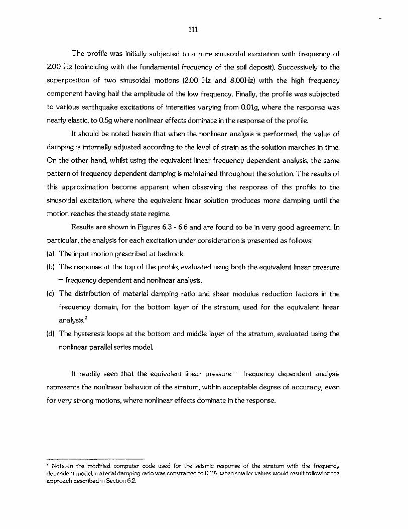
111
The profile was initially subjected to a pure sinusoidal excitation with frequency of
2.00 Hz (coinciding with the fundamental frequency of the soil deposit). Successively to the
superposition of two sinusoidal motions (2.00 Hz and 8.00Hz) with the high frequency
component having half the amplitude of the low frequency. Finally, the profile was subjected
to various earthquake excitations of intensities varying from 0.01g, where the response was
nearly elastic, to 0.5g where nonlinear effects dominate in the response of the profile.
It should be noted herein that when the nonlinear analysis is performed, the value of
damping is internally adjusted according to the level of strain as the solution marches in time.
On the other hand, whilst using the equivalent linear frequency dependent analysis, the same
pattern of frequency dependent damping is maintained throughout the solution. The results of
this approximation become apparent when observing the response of the profile to the
sinusoidal excitation, where the equivalent linear solution produces more damping until the
motion reaches the steady state regime.
Results are shown in Figures 6.3 - 6.6 and are found to be in very good agreement. In
particular, the analysis for each excitation under consideration is presented as follows:
(a) The input motion prescribed at bedrock.
(b) The response at the top of the profile, evaluated using both the equivalent linear pressure
- frequency dependent and nonlinear analysis.
(c) The distribution of material damping ratio and shear modulus reduction factors in the
frequency domain, for the bottom layer of the stratum, used for the equivalent linear
analysis.2
(d) The hysteresis loops at the bottom and middle layer of the stratum, evaluated using the
nonlinear parallel series model.
It readily seen that the equivalent linear pressure - frequency dependent analysis
represents the nonlinear behavior of the stratum, within acceptable degree of accuracy, even
for very strong motions, where nonlinear effects dominate in the response.
2 Note.-In the modified computer code used for the seismic response of the stratum with the frequencydependent model, material damping ratio was constrained to 0.1%, when smaller values would result following theapproach described in Section 6.2.
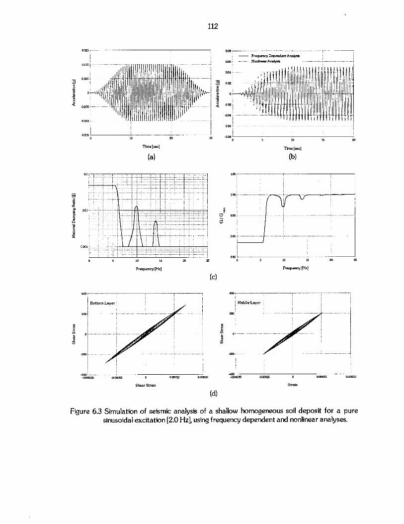
112
0.015
0.010
0.005
0
-0.005
-0.010
-0.015
0
30
Time [sec]
(a)
0.01
0.001
Frequency [Hz]
Bottom Layer
0 -------------------- -------------
-2 0 - ---- - ------- . . - -
T200 -7 -
-00030 -0.00015 0
Shear Strain
0.00015
Time (sec]
(b)
0
U
10 15 20 25
Frequency [Hz]
(c)
(A,
ci,
0.00030
40U,
Middle Layer
200 - - -------- - - - -
Of - --
-200 - --1- ----- - -.-
-400-00030 -0.00015 0 00015 0.000
Strain
0
(d)
Figure 6.3 Simulation of seismic analysis of a shallow homogeneous soil deposit for a puresinusoidal excitation [2.0 Hz], using frequency dependent and nonlinear analyses.
0
113
0.015
0
0 10 20 3
Time [sec]
(a)
-------------- -~ ----- .......
O1
ao - - - -
100~~--- - - -- --- ----
-00-- - -
0 5 10 15 20 25
Frequency [Hz]
200
Bottom Layer
1
Time [sec]
(b)
0
0
10 15 20 25
Frequency [Hz]
(c)
10
-0001 0 01 000062 -0000
Shear Strain
(d)
300
Middle Layer200 -- - -
100 ..
0o---- - ------ ------- ..... - -- -
-100 --
-200 - - - - -
S0e0001 o
Shear Strain
Figure 6.4 Simulation of seismic analysis of a shallow homogeneous soil deposit for thesuperposition of 2 sinusoidal excitations [2.0 and 8.0 Hz], using frequencydependent and nonlinear analyses.
00001 00002
0
-00002
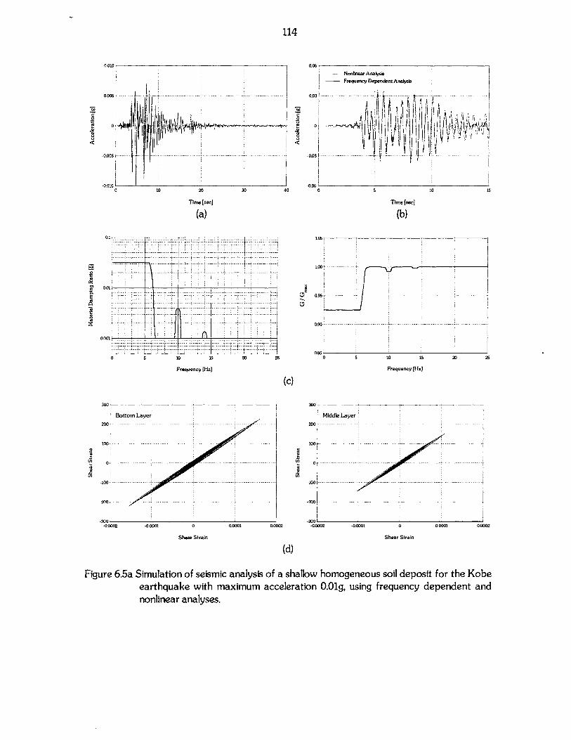
0 10 20 30
Tim [sec]
(a)
.4i
--00--1-
1001 ~ _ _ _ _
0 5 10 15
Frequency [Hz)
25
(c)
-300--0.0002 -0.0001
1.00
0.95 -- - - - -- ---0985
0 5 10 15 20 25
Frequency [Hz]
3001
Middle Layerx .. ...... . ----. ..... ... . ..... . ---
100
U,
U,
0
-100
' -300'-0.0001 0.0002 -00002 -00001
Shear Strain
Figure 6.5a Simulation of seismic analysis of a shallow homogeneous soil deposit for the Kobeearthquake with maximum acceleration 0.01g, using frequency dependent andnonlinear analyses.
114
0.06
.2
.01
'1:
0
.9
40
Time [see]
(b)
15
0,C'EE
X
U)
U,
(d)
0 0.0001 00002
Shear Strain
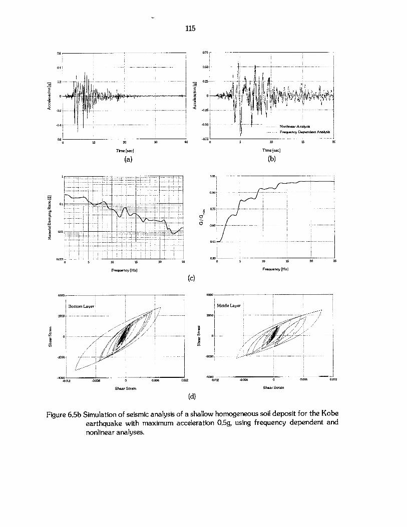
115
0A 4 --- - --- -- ---- ---- - - ------- ------
0 2 1 --- - ... -- -. --. - - - ---- - --- -
0
-02 - --- -- -- ---------- -- - -- - ---- - ---
-0.4 --
0 10 20 30 4
Time [sec]
(a)
001
Frequency [Hz]
4000
Bottom Layer
.0 0 .... .
2000. ----- - ---- -
---- -- ---- -- -- - - - - - -
- 0 -- -- - -- ---- - -- - -- ------ -- -- -
1------ -- ------ - ---000
(10010(10
-0.012
Shear Strain
-.
-0501
0-0.75 0
0.
0.
a
(c)
U)
(0
0.012
205 10 15
Time [sec]
(b)
0 5 10 15 20 2
Frequency [Hz]
4000
Middle Layer
2000-- -----------
-0 --- - -- -- --
-20001 -
-- 006 S
Shear Strain
(d)
Figure 6.5b Simulation of seismic analysis of a shallow homogeneous soil deposit for the Kobeearthquake with maximum acceleration 0.5g, using frequency dependent andnonlinear analyses.
--- -- --- -
5
-002 0.006 0.012-0.006
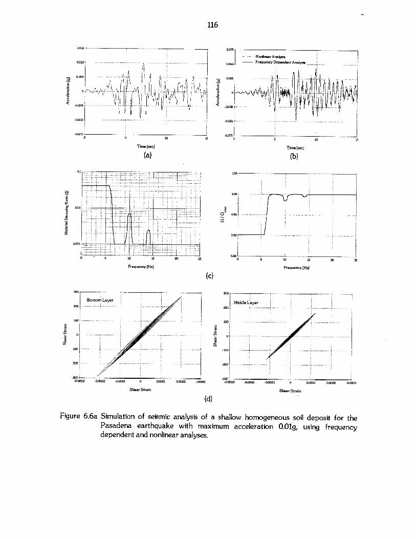
Tne [sec]
(a)
-4. .... ..... .... .... .... ..... ..... ...................... i ; ; -- - i. ..
----- ------- ------ ------
7-- ------ ----
... ..... ....
...........0.01
............ .... .......
7
--- -------...........
QG01
0 5 10 is 20 25
Frequency [Hz)
300o
Bottom Layer200 --- - - ---- - -- - - - - - -- -
100 - -
--- - - -
7 ------------ -
03 -0.0002 -0.0001 0
Shear Strain
300
Middle Layer200 -- - --- --- -
0 -- ---- - -... -- -- --------- -- - ....---
(11-100
-200 -
30003Q00o1 0.0002 0.0003 -00003 -00002 -00001 0
Shear Strain
0.0001 0.0002 00003
(d)
Figure 6.6a Simulation of seismic analysis of a shallow homogeneous soil deposit for thePasadena earthquake with maximum acceleration 0.01g, using frequencydependent and nonlinear analyses.
116
0
-5
15
Time [sec]
(b)
E U
U
(c)
10 15
Frequency [Hz]
20 25
U)
0
-100
-3000-0.00
0
U
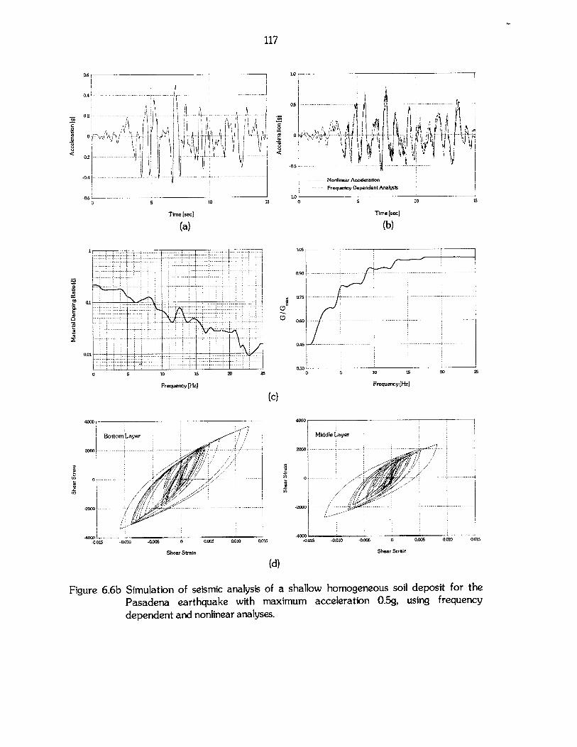
117
15
Time [sec]
(a)
0.1
Frequency [Hz]
4000.-
Bottom Layer
2 0- - ----- - .--
0 ------ ----
-200 -------------- --
00
Time [sec]
(b)
0
Frequency (Hz]
(c)
in)
-005 -amo -O00 050 O 0010 0.015
Shear Strain
(d)
Figure 6.6b SimulationPasadenadependent
4000
Middle Layer
2000 - -- -- -
-2000 - - - -- - -
-4000' --
Shear Strain
of seismic analysis of a shallow homogeneous soil deposit for theearthquake with maximum acceleration 0.5g, using frequencyand nonlinear analyses.
0 0
0.o 0 .10 .1--015 0010 -0os
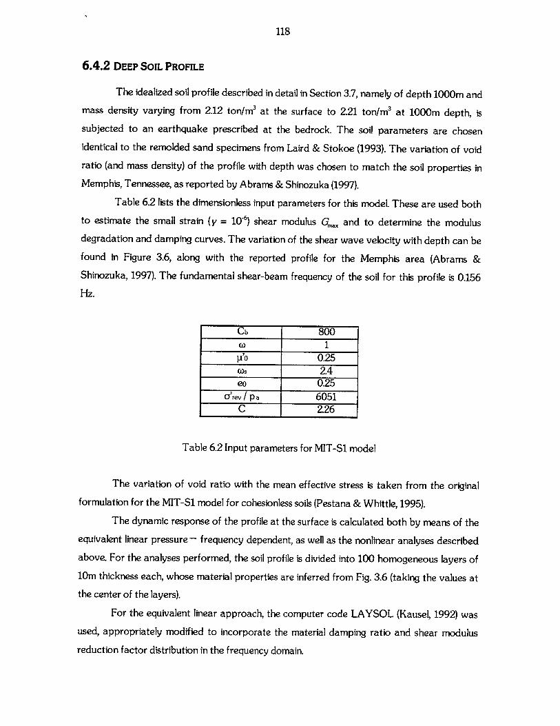
118
6.4.2 DEEP SOIL PROFILE
The idealized soil profile described in detail in Section 3.7, namely of depth 1000m and
mass density varying from 2.12 ton/m3 at the surface to 2.21 ton/m3 at 1000m depth, is
subjected to an earthquake prescribed at the bedrock. The soil parameters are chosen
identical to the remolded sand specimens from Laird & Stokoe (1993). The variation of voidratio (and mass density) of the profile with depth was chosen to match the soil properties in
Memphis, Tennessee, as reported by Abrams & Shinozuka (1997).
Table 6.2 lists the dimensionless input parameters for this model. These are used both
to estimate the small strain (y = 10-6) shear modulus Gm. and to determine the modulus
degradation and damping curves. The variation of the shear wave velocity with depth can be
found in Figure 3.6, along with the reported profile for the Memphis area (Abrams &Shinozuka, 1997). The fundamental shear-beam frequency of the soil for this profile is 0.156
Hz.
Cb 800Ci 1
p'o 0.25os 2.4eo 0.25
a'rev/ p a 6051C 2.26
Table 6.2 Input parameters for MIT-Si model
The variation of void ratio with the mean effective stress is taken from the original
formulation for the MIT-Si model for cohesionless soils (Pestana & Whittle, 1995).
The dynamic response of the profile at the surface is calculated both by means of the
equivalent linear pressure - frequency dependent, as well as the nonlinear analyses described
above. For the analyses performed, the soil profile is divided into 100 homogeneous layers of
10m thickness each, whose material properties are inferred from Fig. 3.6 (taking the values at
the center of the layers).
For the equivalent linear approach, the computer code LAYSOL (Kausel, 1992) was
used, appropriately modified to incorporate the material damping ratio and shear modulus
reduction factor distribution in the frequency domain.
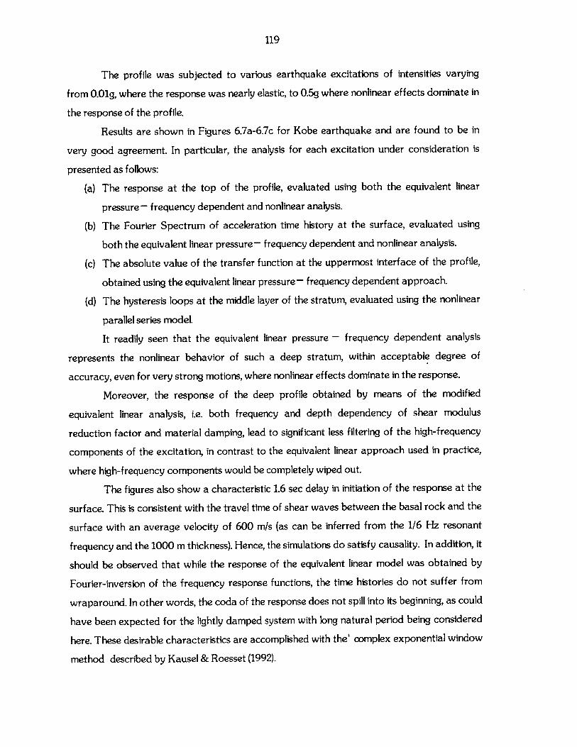
119
The profile was subjected to various earthquake excitations of intensities varying
from 0.01g, where the response was nearly elastic, to 0.5g where nonlinear effects dominate in
the response of the profile.
Results are shown in Figures 6.7a-6.7c for Kobe earthquake and are found to be in
very good agreement. In particular, the analysis for each excitation under consideration is
presented as follows:
(a) The response at the top of the profile, evaluated using both the equivalent linear
pressure - frequency dependent and nonlinear analysis.
(b) The Fourier Spectrum of acceleration time history at the surface, evaluated using
both the equivalent linear pressure- frequency dependent and nonlinear analysis.
(c) The absolute value of the transfer function at the uppermost interface of the profile,
obtained using the equivalent linear pressure- frequency dependent approach.
(d) The hysteresis loops at the middle layer of the stratum, evaluated using the nonlinear
parallel series model.
It readily seen that the equivalent linear pressure - frequency dependent analysis
represents the nonlinear behavior of such a deep stratum, within acceptable degree of
accuracy, even for very strong motions, where nonlinear effects dominate in the response.
Moreover, the response of the deep profile obtained by means of the modified
equivalent linear analysis, i.e. both frequency and depth dependency of shear modulus
reduction factor and material damping, lead to significant less filtering of the high-frequency
components of the excitation, in contrast to the equivalent linear approach used in practice,
where high-frequency components would be completely wiped out.
The figures also show a characteristic 1.6 sec delay in initiation of the response at the
surface. This is consistent with the travel time of shear waves between the basal rock and the
surface with an average velocity of 600 m/s (as can be inferred from the 1/6 Hz resonant
frequency and the 1000 m thickness). Hence, the simulations do satisfy causality. In addition, it
should be observed that while the response of the equivalent linear model was obtained by
Fourier-inversion of the frequency response functions, the time histories do not suffer from
wraparound. In other words, the coda of the response does not spill into its beginning, as could
have been expected for the lightly damped system with long natural period being considered
here. These desirable characteristics are accomplished with the' complex exponential window
method described by Kausel & Roesset (1992).
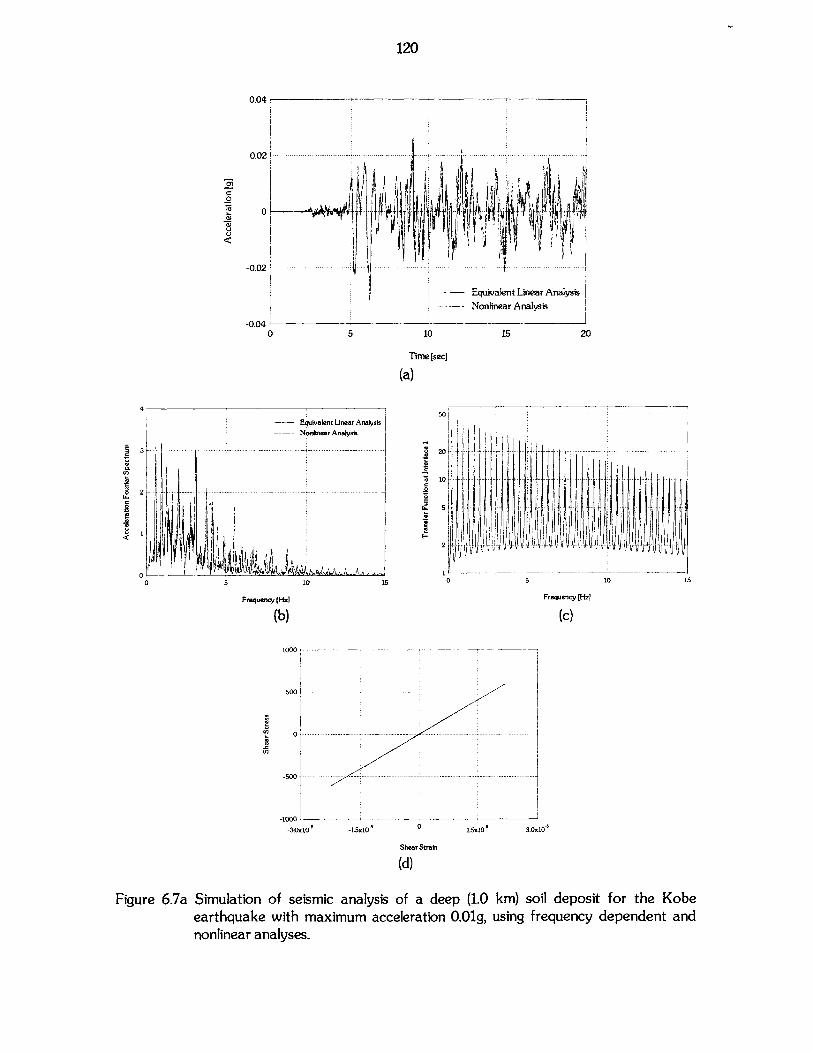
120
0.04
0 .0 2 - - - --- -- - - - - -- - -- -
0 0-
-- Equivalent Linear Analysis
-Nonlinear Analysis
-0.0
0.0 5 10 15 20
Time [sec]
(a)
4Equivalent Linear Analysis-NNonninearlAnalysis
3 -- -- ---- 20 5---- --- -- -- - --
10
2 ~ ~~ o ------------ ----- - - - -
o - - - ---------
-- -- s o - ------ --- --- - - - - --- ------
-15 10 15 1 1.x1 3.1x10~
qukew axu Lnac o .Frequency d
nonlineararaAaalysis
(b) (c)R
1000,
-3.10- -5xlO- 0 1.40_ 3.OxlO-
Shear Strain
(d)
Figure 6.7a Simulation of seismic analysis of a deep (1.0 kin) soil deposit for the Kobeearthquake with maximum acceleration 0.O1g, using frequency dependent andnonlinear analyses.
10 15 20
Time [sec]
(a)
- --- Noninear Anakysis
--- Equivalent UneaT Analysis
Frequency [Hz]
(c)
-0.0001 00001
Shear Strain
(d)
Figure 6.7b Simulation of seismic analysis of a deep (1.0 km)earthquake with maximum acceleration 0.1g, usingnonlinear analyses.
soil deposit for the Kobefrequency dependent and
121
0.4
0.2
00)I)U
-021--
-0.4 -0
15
010
5
10 15
Frequency (Hz]
(b)
15
25001
0
-2500
Li,
-5000 L-0.0003 0.0003
-
5000 ---- -
-------- ----- -- ------- -- ---- -
0
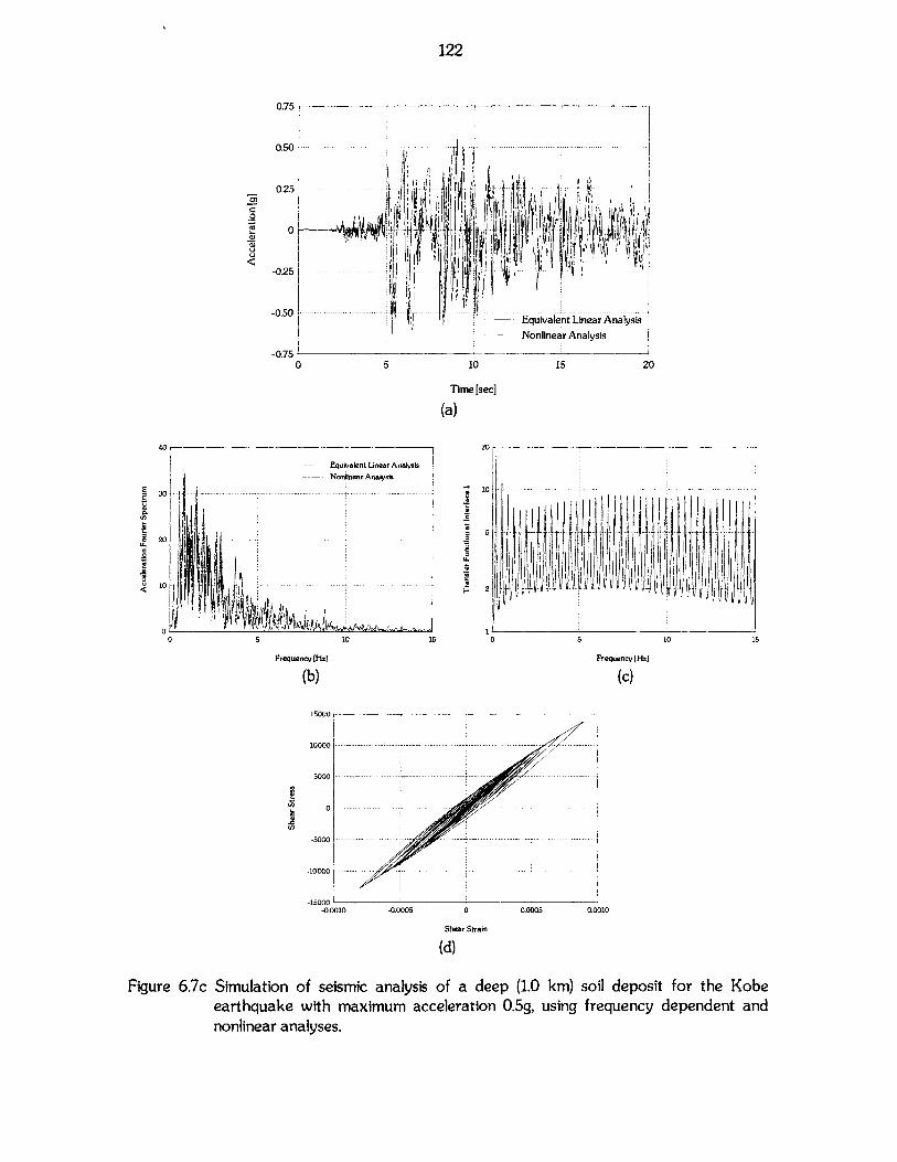
122
0.75
0 .5 - - - -- ---- -- --- ----
02
-0 .2 5 ---- - ---- -- -- - . - ----
Equvaen Lin-a Analysi
- Nonlinear Analysis
-0.750 5 10 15 20
Time [sec]
(a)
40 20
-- Eq- alent Linear AnalysisNonlinear Analysis
E 10 - -- - - - - ----- .---.--
30 .. 10.15.0 5 1 15
1
0 ~ ~~ 5 0 -0 -1 ------ - ---- - - -----------
LL..
1 0 -------------- --.-..-----------------
0 010 15 0 5 10 15
Frequency [iz] Frequency [ d e n a
(b) (c)
15000
0
-15000--0.0010 -0.0005 0 0.0005 0.0010
Shear Strain
(d)
Figure 6.7c Simulation of seismic analysis of a deep (1.0 kin) soil deposit for the Kobe
earthquake with maximum acceleration 0.5g, using frequency dependent and
nonlinear analyses.
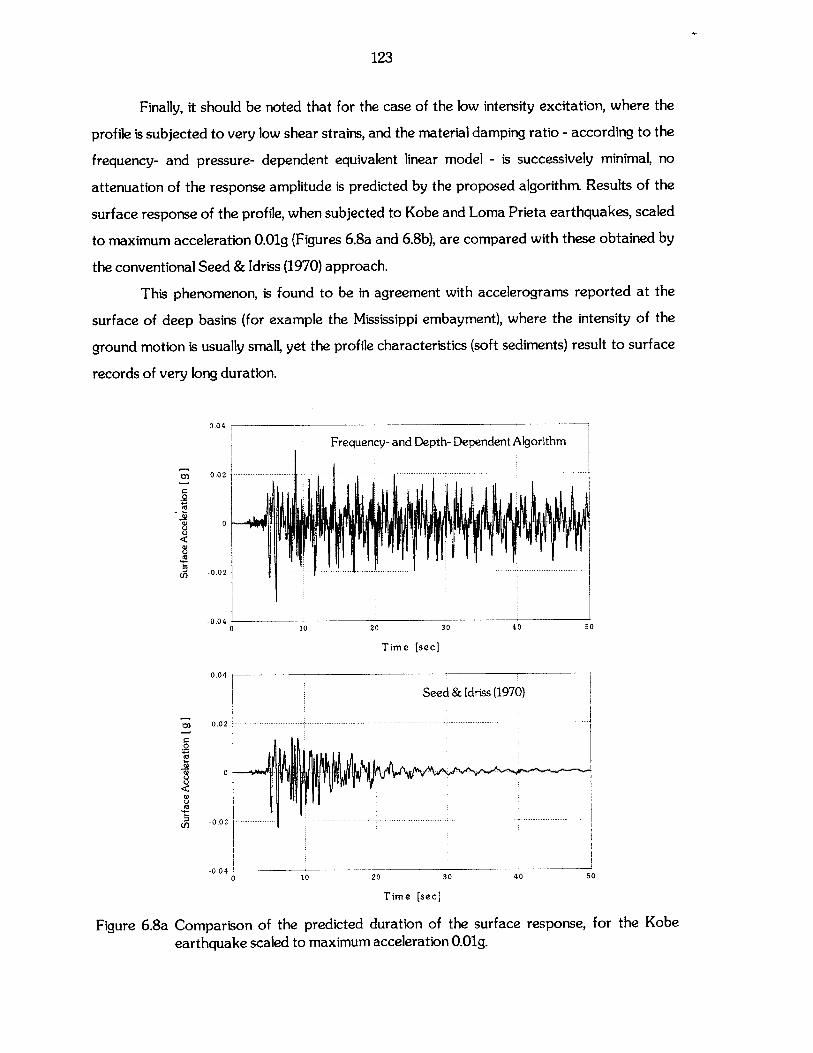
123
Finally, it should be noted that for the case of the low intensity excitation, where the
profile is subjected to very low shear strains, and the material damping ratio - according to the
frequency- and pressure- dependent equivalent linear model - is successively minimal, no
attenuation of the response amplitude is predicted by the proposed algorithm. Results of the
surface response of the profile, when subjected to Kobe and Loma Prieta earthquakes, scaled
to maximum acceleration 0.01g (Figures 6.8a and 6.8b), are compared with these obtained by
the conventional Seed & Idriss (1970) approach.
This phenomenon, is found to be in agreement with accelerograms reported at the
surface of deep basins (for example the Mississippi embayment), where the intensity of the
ground motion is usually small, yet the profile characteristics (soft sediments) result to surface
records of very long duration.
10 20 30
Time [sec]
40
10 20 30 40
Time [sec]
Figure 6.8a Comparison of the predicted duration of the surface response, for the Kobeearthquake scaled to maximum acceleration 0.01g.
Frequency- and Depth- Dependent Algorithm
------------ -- - -- ---- --- -------- ---- -- -- --- --- ------------ ------
--- ---- -- -- - - -- ------ -------- -- - - - ----- --- - --- - ---- ----- - - -- ----
0.04
0.02
0
-0.02
-0.040
0
wC.,C.,
C.,
0
Cl)
0)
0
C-)
w0
(12
0.04
0.02
0
-0.02
-0.04 0
50
50
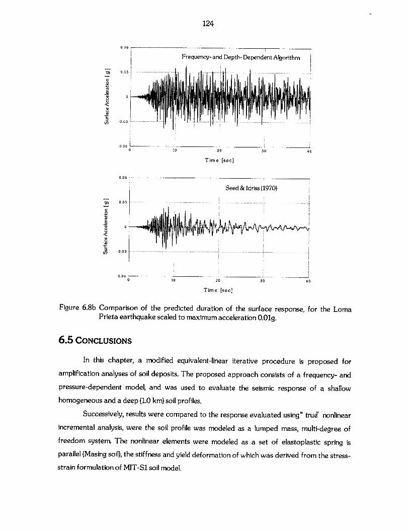
124
0.06
Frequency- and Depth- Dependent Algorithm
0 .0 3 -- - - - -- - - -- -- -- - --- - --- --- - - -- -- - - -- - - -- - -- - -- - -- - - -- - -- -
0
-0.060 10 20 30 40
Time [sec]
0.06
Seed & Idriss (1970)
0 .0 3 -- - --- - ------------ - - -- - -- ----- - --- - - - - --- --- - - -- - - -- -- - -- - - --- -- -- - -- -
0 0
-0 .0 3 -- ---- ---- ------- - ----- ------ --- - ---- -- ------ - ----- -- - ------ - - - --- - ---- --- - - - -- -- - -- - - --
-0.060 10 20 30 40
Time [sec]
Figure 6.8b Comparison of the predicted duration of the surface response, for the LomaPrieta earthquake scaled to maximum acceleration 0.01g.
6.5 CONCLUSIONS
In this chapter, a modified equivalent-linear iterative procedure is proposed for
amplification analyses of soil deposits. The proposed approach consists of a frequency- and
pressure-dependent model, and was used to evaluate the seismic response of a shallow
homogeneous and a deep (1.0 km) soil profiles.
Successively, results were compared to the response evaluated using" true nonlinear
incremental analysis, were the soil profile was modeled as a Jumped mass, multi-degree of
freedom system. The nonlinear elements were modeled as a set of elastoplastic spring is
parallel (Masing soil), the stiffness and yield deformation of which was derived from the stress-
strain formulation of MIT-Sl soil model.
125
The profiles were subjected to various excitations, with amplitudes varying from 0.01g
(nearly elastic behavior) to 0.5g (very pronounced nonlinear response). Results were found to
be in very good agreement, both for the shallow homogeneous as well as for the deep soil
profiles.
Moreover, as it was expected, the seismic amplification analysis evaluated in the
frequency - wavenumber domain, by means of a continuum formulation of the wave
propagation problem, demands significantly less computational effort than the incremental
analysis. In particular, a considerably lower time step is required for the conditionally stable
direct integration scheme used for the present study, namely the central difference method, to
allow for an accurate representation of the resonant frequencies of the profile, a fact which
becomes more apparent as the depth and / or the shear wave velocity of the profile analyzed
increases.
The proposed algorithm represents within acceptable degree of accuracy the
nonlinear soil behavior and prevents the artificial filtering of the high-frequency components of
the excitation.
6.6 REFERENCES
Assimaki, D., Kausel, E. & Whittle, A.J. (1999)." A Model for Dynamic Shear Modulus andDamping for Granular Soils , Journal of Geotechnical and GeoenvironmentalEngineering, under publication
Constantopoulos, I. V. (1973)." Amplification Studies for a Nonlinear Hysteretic Soil Model',Research Report R73-46, Massachusetts Institute of Technology, September
Constantopoulos, I. V., Roesser, J. M. & Christian, J. T. A. (1973)." Comparison of linear andexact nonlinear analyses of soil amplification , Proc. 5 h World Conference onEarthquake Engineering, Rome
Dames & Moore, Science Applications Inc. (1978). " Study of Nonlinear Effects on One -Dimensional Earthquake Response, prepared for Electric Power Research Institute,Projects 615-1,-2
Hall, J. R. Jr. & Richard, F. E. Jr. (1963). " Dissipation of Elastic Wave Energy in GranularSoils ,Journal of the Soil Mechanics and Foundation Division, ASCE, Vol. 98, No. SM6,November, pp. 27-56
Joyner, W. B. & Chen, A. T. F. (1975). " Calculation of Non-linear Ground Response inEarthquakes , Bulletin of the Seismological Society of America, Vol. 65, No. 5, October,pp. 1315-1336
Kausel,E. (1992)." LAYSOL: A computer program for the dynamic analysis of layered soil'Kausel,E. & Roesset, J.M. (1992)." Frequency domain analysis of undamped systems using the
exponential window method' , Proc. 10th World Conference on Earthquake Engineering,Madrid, Spain
126
Roesset, J.M & Whitman, R.V. (1969)." Theoretical Background for Amplification Studie ,Research Report R69-15, Massachusetts Institute of Technology, Soils Publication No.231, March
Whitman, R. V. (1970). " Evaluation of Soil Properties for Site Evaluation and DynamicAnalysis of Nuclear Plants , Seismic Design for Nuclear Plants, R. J. Hanson (ed.), MITPress, Cambridge, Massachusetts

127
APPENDICES

128
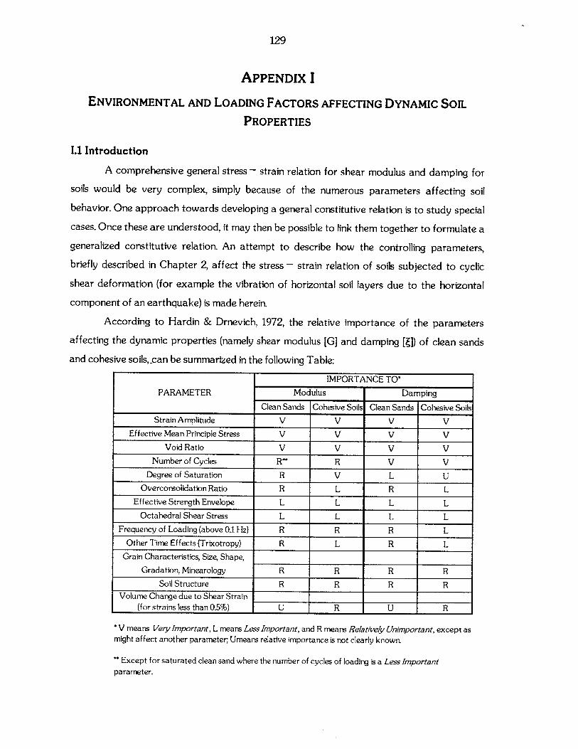
129
APPENDIX I
ENVIRONMENTAL AND LOADING FACTORS AFFECTING DYNAMIC SOIL
PROPERTIES
1.1 Introduction
A comprehensive general stress - strain relation for shear modulus and damping for
soils would be very complex, simply because of the numerous parameters affecting soil
behavior. One approach towards developing a general constitutive relation is to study special
cases. Once these are understood, it may then be possible to link them together to formulate a
generalized constitutive relation. An attempt to describe how the controlling parameters,
briefly described in Chapter 2, affect the stress - strain relation of soils subjected to cyclic
shear deformation (for example the vibration of horizontal soil layers due to the horizontal
component of an earthquake) is made herein.
According to Hardin & Drnevich, 1972, the relative importance of the parameters
affecting the dynamic properties (namely shear modulus [G] and damping [ ]) of clean sands
and cohesive soils,.can be summarized in the following Table:
IMPORTANCE TO*
PARAMETER Modulus Damping
Clean Sands Cohesive Soils Clean Sands Cohesive SoilsStrain Amplitude V V V V
Effective Mean Principle Stress V V V VVoid Ratio V V V V
Number of Cycles R** R V VDegree of Saturation R V L U
Overconsolidation Ratio R L R L
Effective Strength Envelope L L L L
Octahedral Shear Stress L L L LFrequency of Loading (above 0.1 Hz) R R R L
Other Time Effects (Trixotropy) R L R L
Grain Characteristics, Size, Shape,
Gradation, Minearology R R R R
Soil Structure R R R RVolume Change due to Shear Strain
(for strains less than 0.5%) U R U R
* V means Very Important, L means Less Important, and R means Relatively Unimportant, except asmight affect another parameter; Umeans relative importance is not clearly known.
** Except for saturated clean sand where the number of cycles of loading is a Less Importantparameter.
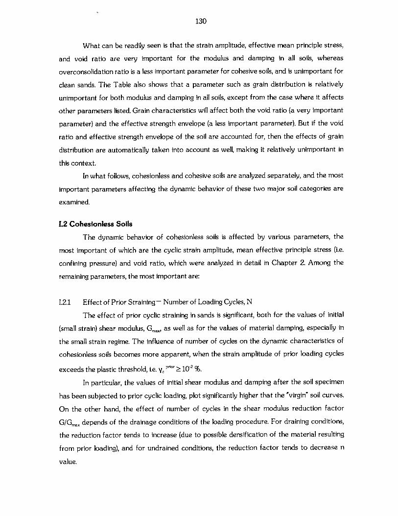
130
What can be readily seen is that the strain amplitude, effective mean principle stress,
and void ratio are very important for the modulus and damping in all soils, whereas
overconsolidation ratio is a less important parameter for cohesive soils, and is unimportant for
clean sands. The Table also shows that a parameter such as grain distribution is relatively
unimportant for both modulus and damping in all soils, except from the case where it affects
other parameters listed. Grain characteristics will affect both the void ratio (a very important
parameter) and the effective strength envelope (a less important parameter). But if the void
ratio and effective strength envelope of the soil are accounted for, then the effects of grain
distribution are automatically taken into account as well, making it relatively unimportant in
this context.
In what follows, cohesionless and cohesive soils are analyzed separately, and the most
important parameters affecting the dynamic behavior of these two major soil categories are
examined.
1.2 Cohesionless Soils
The dynamic behavior of cohesionless soils is affected by various parameters, the
most important of which are the cyclic strain amplitude, mean effective principle stress (i.e.
confining pressure) and void ratio, which were analyzed in detail in Chapter 2. Among the
remaining parameters, the most important are:
1.2.1 Effect of Prior Straining - Number of Loading Cycles, N
The effect of prior cyclic straining in sands is significant, both for the values of initial
(small strain) shear modulus, Gm., as well as for the values of material damping, especially in
the small strain regime. The influence of number of cycles on the dynamic characteristics of
cohesionless soils becomes more apparent, when the strain amplitude of prior loading cycles
exceeds the plastic threshold, i.e. y P" > 10 2%.
In particular, the values of initial shear modulus and damping after the soil specimen
has been subjected to prior cyclic loading, plot significantly higher that the "virgin" soil curves.
On the other hand, the effect of number of cycles in the shear modulus reduction factor
G/Gmax depends of the drainage conditions of the loading procedure. For draining conditions,
the reduction factor tends to increase (due to possible densification of the material resulting
from prior loading), and for undrained conditions, the reduction factor tends to decrease n
value.
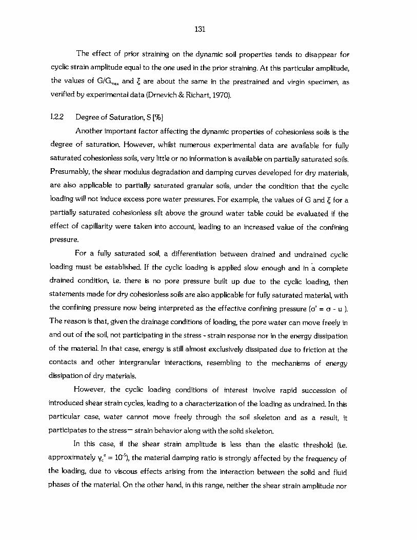
131
The effect of prior straining on the dynamic soil properties tends to disappear for
cyclic strain amplitude equal to the one used in the prior straining. At this particular amplitude,
the values of G/Gmax and Z are about the same in the prestrained and virgin specimen, as
verified by experimental data (Drnevich & Richart, 1970).
1.2.2 Degree of Saturation, S [%]
Another important factor affecting the dynamic properties of cohesionless soils is the
degree of saturation. However, whilst numerous experimental data are available for fully
saturated cohesionless soils, very little or no information is available on partially saturated soils.
Presumably, the shear modulus degradation and damping curves developed for dry materials,
are also applicable to partially saturated granular soils, under the condition that the cyclic
loading will not induce excess pore water pressures. For example, the values of G and Z for a
partially saturated cohesionless silt above the ground water table could be evaluated if the
effect of capillarity were taken into account, leading to an increased value of the confining
pressure.
For a fully saturated soil, a differentiation between drained and undrained cyclic
loading must be established. If the cyclic loading is applied slow enough and in a complete
drained condition, i.e. there is no pore pressure built up due to the cyclic loading, then
statements made for dry cohesionless soils are also applicable for fully saturated material, with
the confining pressure now being interpreted as the effective confining pressure (a' = a - u ).
The reason is that, given the drainage conditions of loading, the pore water can move freely in
and out of the soil, not participating in the stress - strain response nor in the energy dissipation
of the material. In that case, energy is still almost exclusively dissipated due to friction at the
contacts and other intergranular interactions, resembling to the mechanisms of energy
dissipation of dry materials.
However, the cyclic loading conditions of interest involve rapid succession of
introduced shear strain cycles, leading to a characterization of the loading as undrained. In this
particular case, water cannot move freely through the soil skeleton and as a result, it
participates to the stress- strain behavior along with the solid skeleton.
In this case, if the shear strain amplitude is less than the elastic threshold (i.e.
approximately y = 10-5), the material damping ratio is strongly affected by the frequency of
the loading, due to viscous effects arising from the interaction between the solid and fluid
phases of the material. On the other hand, in this range, neither the shear strain amplitude nor
132
the number of cycles, affect the dynamic soil properties. If the shear strain amplitude is larger
than the elastic threshold, but still smaller than the volumetric threshold (i.e. approximately
y;'= 10-'), the role of frequency on the value of material damping becomes less important, and
the value of the shear modulus reduction factor is approximately equal to the one established
for the dry material.
In essence, between the two thresholds, the level of strain amplitude is important but
the number of cycles not. On the other hand, if the shear strain amplitude is larger than the
volumetric threshold, then the effect of frequency on the dynamic properties of the material
becomes negligible, and the value of shear modulus decreases with increasing strain amplitude
and number of cycles.
This phenomenon of shear modulus degradation, which can reduce the value of G to a
value close to zero, is due to the built up of excess pore pressures in the soil, an extreme
example of which being the phenomenon of liquefaction of saturated cohesionless soils. The
value of material damping ratio, whilst pore pressure built - up occurs with increasing number
of cycles, remains constant or decreases (Dobry, et al. 1982, Stokoe, et al., 1995, Vucetic, et al.,
1996).
In conclusion, the behavior of saturated cohesionless soils described above indicates
that there is no substantial difference between the dynamic properties of a saturated soil and
a dry soil under similar confining pressure. Therefore, the effect of excess pore pressure in
decreasing G/Gmax can be explained by the corresponding reduction in effective confining
pressure. However, for high frequency cyclic loading such as applied in resonant column tests,
and for small cyclic strains, the material damping is higher for the saturated sand, due to
viscous effects related to the relative movements involving solid phase and pore water, which
essentially become insignificant at greater cyclic strains. Therefore, the difference in damping
between dry and saturated soil is generally more important when high - vibration phenomena
are encountered, such as machine vibrations or explosions.
1.2.3 Effect of Cementation
The cementation of a cohesionless material, either natural or artificial, increases both
the small- strain shear modulus Gmax, as well as the small- strain material damping value, Zmn.
Strong cementation also decreases the significance of confining pressure. It may also radically
change the shapes of the modulus reduction and damping curves, by decreasing the relative
importance of friction at the interparticle contacts and the freedom of movement of the
133
grains. In particular, the stress - strain relationship of the material becomes more linear, a fact
which becomes more apparent in the small - strain regime and might even disappear at cyclic
strain amplitudes large enough to destroy the cementation. At those high strain amplitudes,
the dynamic properties of the cemented material may approach the uncemented values, with
the shear modulus degradation curve of the remolded material even plotting lower than the
equivalent uncemented.
1.3 Cohesive Soils
Probably the most important parameter affecting the dynamic behavior of cohesive
soils apart from the shear strain amplitude, is the plasticity index [PI]. Parameters as the
overconsolidation ratio or confining pressure play minor role in this category of soils. In what
follows, various parameters apart from the Plasticity Index, namely the number of straining
cycles and the geological age of the material, are further analyzed, and experimental formulae
existing in the literature for the estimation of material damping and shear modulus reduction
factor as a function of these parameters are briefly discussed.
1.3.1 Effect of Plasticity Index [PI]
Numerous experimental data, available in the literature, reveal the importance of
plasticity index in the characterization of the dynamic properties of cohesive soils. In the early
years of geotechnical earthquake engineering, the modulus reduction behavior of coarse- and
fine- grained soils were treated separately (e.g., Seed & Idriss, 1970). Recent research however,
has revealed a gradual transition between the modulus reduction behavior of non-plastic
coarse-grained (cohesionless) soil and plastic fine-grained (cohesive) soil.
Zen et al. (1978) and Kokushu et al. (1982) first noted the influence of soil plasticity on
the shape of the modulus reduction curves; the shear modulus of highly plastic soils was
observed to degrade more slowly with shear strain than did low-plasticity soils. Laboratory
data show that the linear cyclic threshold shear strain is greater for highly plastic soils than for
soils with low plasticity. Moreover, for non-plastic cohesive soils such as non-plastic silt, the
shear modulus reduction curves plot together with the non-cohesive soil curves.
After reviewing experimental results from a broad range of materials, Dobry &
Vucetic (1987) and Sun et al. (1988) concluded that the shape of the modulus reduction curve
is influenced more by the Plasticity Index than by the void ratio and/or the confining pressure.
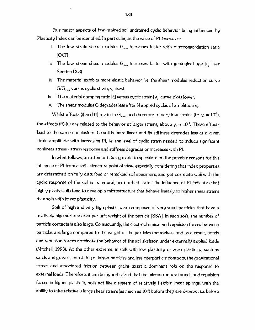
134
Five major aspects of fine-grained soil undrained cyclic behavior being influenced by
Plasticity Index can be identified. In particular, as the value of PI increases:
i. The low strain shear modulus Gmax increases faster with overconsolidation ratio
[OCR].
ii. The low strain shear modulus Gm increases faster with geological age [tg] (see
Section 1.3.3).
iii. The material exhibits more elastic behavior (i.e. the shear modulus reduction curve
G/Gma versus cyclic strain, ye rises).
iv. The material damping ratio [Z] versus cyclic strain [yc] curve plots lower.
v. The shear modulus G degrades less after N applied cycles of amplitude yc.
Whilst effects (i) and (ii) relate to Gmax, and therefore to very low strains (i.e. ye ~ 10-6)
the effects (iii)-(v) are related to the behavior at larger strains, above ye ~ 107. These effects
lead to the same conclusion: the soil is more linear and its stiffness degrades less at a given
strain amplitude with increasing PI, i.e. the level of cyclic strain needed to induce significant
nonlinear stress - strain response and stiffness degradation increases with PI.
In what follows, an attempt is being made to speculate on the possible reasons for this
influence of PI from a soil - structure point of view, especially considering that index properties
are determined on fully disturbed or remolded soil specimens, and yet correlate well with the
cyclic response of the soil in its natural, undisturbed state. The influence of PI indicates that
highly plastic soils tend to develop a microstructure that behave linearly to higher shear strains
than soils with lower plasticity.
Soils of high and very high plasticity are composed of very small particles that have a
relatively high surface area per unit weight of the particle [SSA]. In such soils, the number of
particle contacts is also large. Consequently, the electrochemical and repulsive forces between
particles are large compared to the weight of the particles themselves, and as a result, bonds
and repulsion forces dominate the behavior of the soil skeleton under externally applied loads
(Mitchell, 1993). At the other extreme, in soils with low plasticity or zero plasticity, such as
sands and gravels, consisting of larger particles and less interparticle contacts, the gravitational
forces and associated friction between grains exert a dominant role on the response to
external loads. Therefore, it can be hypothesized that the microstructural bonds and repulsion
forces in higher plasticity soils act like a system of relatively flexible linear springs, with the
ability to take relatively large shear strains (as much as 10-3) before they are broken, i.e. before
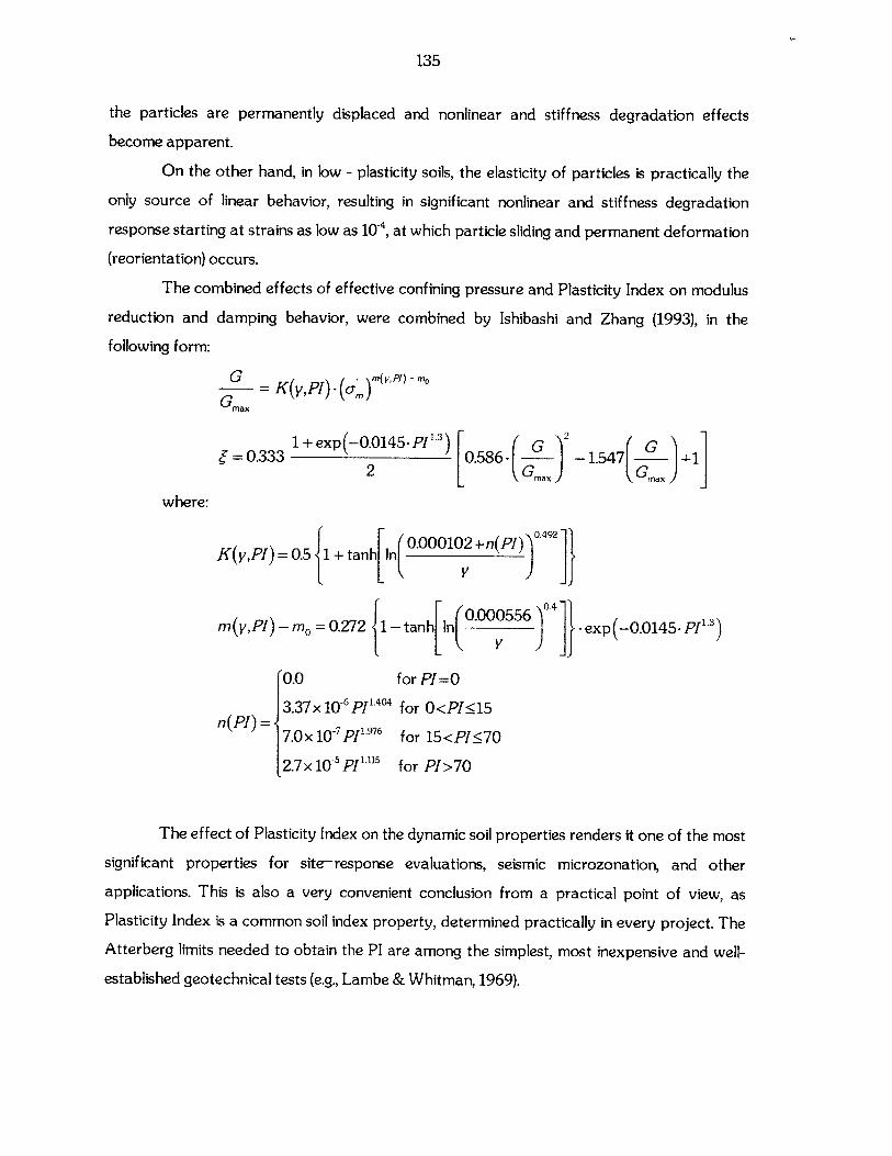
135
the particles are permanently displaced and nonlinear and stiffness degradation effects
become apparent.
On the other hand, in low - plasticity soils, the elasticity of particles is practically the
only source of linear behavior, resulting in significant nonlinear and stiffness degradation
response starting at strains as low as 10~4, at which particle sliding and permanent deformation
(reorientation) occurs.
The combined effects of effective confining pressure and Plasticity Index on modulus
reduction and damping behavior, were combined by Ishibashi and Zhang (1993), in the
following form:
G K(y,P) )m(VPI ) - mGmax
1 +exp(-0.0145.PI"-) G 2 G2=0.333 0.586 - -1.547 +12 G ) CGID ]
where:
K(y,PI) = 0.5 1 + tanh In 0.000102+n(PI)
m(y,PI) - m= 0.272 1- tanh In j 0 exp(-0.0145. P1 3 )
'0.0 for PI=0
3.37 x 10⁻⁶ p1404 for 0<PI 15n (M) =17.0 x 10⁻⁷ P 9 76 for 15 <P1 70
2.7x 10~ PI"'5 for PI>70
The effect of Plasticity Index on the dynamic soil properties renders it one of the most
significant properties for site-response evaluations, seismic microzonation, and other
applications. This is also a very convenient conclusion from a practical point of view, as
Plasticity Index is a common soil index property, determined practically in every project. The
Atterberg limits needed to obtain the PI are among the simplest, most inexpensive and well-
established geotechnical tests (e.g., Lambe & Whitman, 1969).
136
1.3.2 Number of Loading Cycles, N
Similarly to the behavior of cohesionless soils, the stiffness of a saturated cohesive soil
decreases with number of cycles when subjected to undrained cyclic loading. The degradation
of shear modulus G is accompanied by interparticle bond breakage and pore pressure built-
up, with the rate of modulus degradation with number of cycles, for a given strain amplitude,
decreasing with increasing Plasticity Index. Even for low plasticity cohesive soils, this rate is
much smaller than for saturated sands, and for a small number of cycles, results from a single
loading - unloading - reloading path can be used without modification.
For large amount of straining cycles (N> 102 - 10), the shear modulus after N cycles,
GN can be related to its value in the first cycle G1 as follows:
GN=6 -G1,
where the degradation index, 5, is obtained as 6 = Nt and t is the degradation parameter
(Idriss et al., 1978). The degradation parameter has been shown to decrease with increasing
Plasticity Index and increasing OCR, and to increase with increasing cyclic strain amplitude
(Idriss et al., 1978, Vucetic & Dobry, 1989, Tan & Vucetic, 1989).
1.3.3 Effect of Geologic Age, t.Another factor affecting the dynamic soil properties of cohesive soils is the time of
loading. In particular, the small - strain shear modulus Gmax increases with time of loading and
material damping ratio Z decreases. This is part of the explanation of why older geologic
deposits tend to be stiffer (higher Gm. and V, values), and the effect must be considered when
predicting Gma. and V, values from laboratory measurements. This effect is also present in the
secant shear modulus G at larger cyclic strains.
Experimental data on the influence of time of loading on the shear modulus
degradation curve is not conclusive, and two different procedures have been proposed to
estimate the secant shear modulus of the field (Gf,) from the corresponding measured in the
lab using a short loading time (Glab). Some laboratory data suggests that time of loading affects
Gmax but not the G/Gmax versus V curve, and Kokusho et al. (1982) have proposed to correct G
measured in the lab, as follows:
Gfigd = (Gmax)f i. x (G / Ga)ab
where (Gma.)i, is the corrected value of the small shear strain shear modulus.
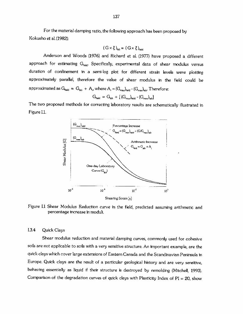
137
For the material damping ratio, the following approach has been proposed by
Kokusho et al. (1982):
(G x ( )Ia= (G x Z)filAnderson and Woods (1976) and Richard et al. (1977) have proposed a different
approach for estimating Gfi. Specifically, experimental data of shear modulus versus
duration of confinement in a semi-log plot for different strain levels were plotting
approximately parallel, therefore the value of shear modulus in the field could be
approximated as Gf. ~ Glab + Ar, where A, = (Gm.jf - (G.)ab. Therefore:
Gfie = Glab + [(Gm.)fi - (Gma),ab]
The two proposed methods for correcting laboratory results are schematically illustrated in
Figure 1.1.
(G )field Percentage Increase
G = (G) x (G/G )ab
(G )aArithmetic Increase
G =Gia+A
-0
One-day Laboratory
Curve (Giad
10-6 104 102 100
Shearing Strain [y]
Figure 1.1 Shear Modulus Reduction curve in the field, predicted assuming arithmetic andpercentage increase in moduli.
1.3.4 Quick Clays
Shear modulus reduction and material damping curves, commonly used for cohesive
soils are not applicable to soils with a very sensitive structure. An important example, are the
quick clays which cover large extensions of Eastern Canada and the Scandinavian Peninsula in
Europe. Quick clays are the result of a particular geological history and are very sensitive,
behaving essentially as liquid if their structure is destroyed by remolding (Mitchell, 1993).
Comparison of the degradation curves of quick clays with Plasticity Index of PI = 20, show
138
correspondence to a regular clay with PI = 50, while the values of material damping
correspond to a regular clay with PI ~ 200. This results from the unusual structure of this
particular soil type, which can exhibit more linear behavior, including a much lower material
damping, than would have been predicted from its Plasticity Index.
1.4 Other Soils
In the preceding sections, parameters affecting the shear modulus and material
damping values for applications over a broad range of cohesive and cohesionless soils have
been analyzed. However, some characteristics of the materials described above may not be
applicable to so called special soils and other geotechnical materials of interest having a very
different composition or structure as compared with the normal soils.
Laboratory measurements and analysis of earthquake records have provided
valuable information on the shapes of modulus and damping curves for some of these special
geotechnical materials of interest.
In some cases, like that of frozen soils, the cyclic stress - strain behavior is quite
complicated and is strongly affected by parameters such as temperature and frequency.
Experimental evidence for one marine calcareous soil near Western Australia indicates that
the shear modulus degradation curves, G/Gmax, characteristic for sands are applicable for this
particular material as well, whilst the wide variety of calcareous soils, both onshore as well as
offshore suggests that no generalization is possible.
Among other geotechnical materials of interest, soft rock and residual soils, peat and
solid waste could be distinguished due to their irregular soil behavior. Comparison of
experimental data obtained in two different projects in New York City and Washington State
indicate that peats can exhibit both a very linear stress - strain response, accompanied by very
low values of material damping, and significant non-linearity, associated with substantial
amount of energy dissipation.
1.5 References
Anderson, D.G. & Woods, R.D. (1976)." Comparison of field and laboratory shear modulus ,Proc. ASCE Conference on In-situ Measurement of Soil Properties, Vol.1, pp. 62-92.
Chen, A. T. F., Stokoe, K. H., 11 (1979). "Interpretation of Strain Dependent Modulus andDamping from Torsional Soil Tests", Report No. USGS - GD - 79 - 002, NTIS NO. PB -298479, U.S. Geological Survey, 46 P.
139
Daniel, A. W. T., Harvey, R. C. and Burley, E. (1975). "Stress - Strain Characteristics of Sand",Technical Note, Journal of the Geotechnical Division, ASCE, Vol.101, No. GT5, May, pp.508-512
Das, B. M. (1993). "Principles of Soil Dynamics", PWS-KENT Publishing Company, Boston, MADobry, R., Ladd, R.S., Yokel, F.Y., Chung, R.M. & Powell, D. (1982). "Prediction of pore water
pressure buildup and liquefaction of sands during earthquakes using the cyclic strainmethod", NBS Building Science Series 138, National Bureau of Standards, Gaithersburg,Maryland
Dobry, R. & Vucetic, M. (1987). " Dynamic Properties and Seismic Response of soft claydeposits' , Proc. International Symposium on Geotechnical Engineering of Soft Sois,Mexico City, Vol. 2, pp. 51-87
Drnevich, V.P. & Richard, F.E. Jr. (1970)." Dynamic Prestraining of Dry Sand' , Journal of theSoil Mechanics and Foundations Division, ASCE, Vol. 98, No. SM8, pp. 807-825.
Finn, W. D. L., Lee, K. W. & Martin, G. R. (1975)." Stress-Strain Relations for Sand in SimpleSheaf , ASCE National Convention, Denver, Colorado, November, Meeting Reprint 2517
Hall, J. R. Jr. & Richard, F. E. Jr. (1963). " Dissipation of Elastic Wave Energy in GranularSoils' ,Journal of the Soil Mechanics and Foundation Division, ASCE, Vol. 98, No. SM6,November, pp. 27-56
Hardin, B. 0. (1965). "The nature of damping in sands", Journal of Soil Mechanics andFoundation Engineering Division, ASCE, Vol. 91, No. SM1, February, pp. 33-65.
Hardin, B. 0. & Drnevich, V. P. (1970)." Shear modulus and damping in soils: I. Measurementand parameter effects, II. Design equations and curves' , Technical Reports UKY 27-70-CE 2 and 3, College of Engineering, University of Kentucky, Lexington, Kentucky.
Hardin, B. 0. & Drnevich, V. P. (1972a)." Shear modulus and damping in soils: Measurementand parameter effects', Journal of Soil Mechanics and Foundation EngineeringDivision, ASCE, Vol. 98, No. SM6, June, pp. 603-624.
Hardin, B. 0. & Drnevich, V. P. (1972b)." Shear modulus and damping in soils: Design equationsand curves", Journal of Soil Mechanics and Foundation Engineering Division, ASCE,Vol. 98, No. SM7, pp. 667-692.
Ishibashi, I. & Zhang, X. (1993)." Unified Dynamic Shear Moduli and Damping Ratios of Sandand Clay' , Soils and Foundations, Vol. 33, No.1, pp. 182-191.
Ishihara, K. (1996). "Soil Behavior in Earthquake Geotechnics", Oxford Science Publications,Oxford Science Press, Walton Street, Oxford OX2 6DP.
Iwasaki, T., Tatsuoka, F. & Takagi, Y. (1978). "Shear Moduli of Sands under Cyclic TorsionalShear Loading", Soils and Foundations, Vol. 18, No.1, pp. 39-56.
Kramer, K. L. (1996)." Geotechnical Earthquake Engineering , Prentice Hall Inc.Kokushu, T., Yoshida, Y. & Esashi, Y. (1982)." Dynamic Properties of Soft Clay for wide strain
rang' , Soils and Foundations, Vol. 22, No.2, pp. 45-60.Krizek, R. J. & Franklin, A. G. (1968)." Energy Dissipation in a Soft Clay', Proc. International
Symposium on Wave Propagation and Dynamic Properties of Earth Materials,University of New Mexico, pp. 797-807.
140
Laird, J. P. & Stokoe, K. H. (1993)." Dynamic properties of remolded and undisturbed soilsamples tested at high confining pressured', Geotechnical Engineering Report GR93-6,Electrical Power Research Institute.
Lambe, T.W. & Whitman, R.V. (1969). Soil Mechanics, Wiley, New York.Mitchell, J.K. (1993)." Fundamentals of Soil Behavior , John Wiley & Sons, Inc.Ray, R. P. & Woods, R. D. (1988)," Modulus and Damping due to uniform and variable cyclic
loading' , Journal of Geotechnical Engineering, ASCE, 114 (8), pp. 861-876.Seed, H. B. & Idriss, I. M. (1970), " Soil moduli and damping factors for dynamic response
analyses', Report EERC 70-10, Earthquake Research Center, University of California,Berkeley.
Seed, H. B., Wong R. T., Idriss, I. M. & Tokimatsu T. (1984)," Moduli and damping factors fordynamic analyses of cohesionless soils' , Report EERC 84-14, Earthquake EngineeringResearch Center, University of California, Berkeley.
Seed, H. B., Wong R. T., Idriss, I. M. & Tokimatsu T. (1986)," Moduli and damping factors fordynamic analyses of cohesionless soilV', Journal of Soil Mechanics and FoundationDivision, ASCE, Vol. 112, No. SM11, pp. 1016-1032.
Shibata, T. & Soelarno, D. S. (1975), " Stress strain characteristics of sands under cyclicloading' , Proc.. Japanese Society of Civil Engineering, 239, pp. 57-65.
Shibuya, S., Mitachi, T. & Muira, S. (1994). "Pre-failure Deformation of Geomaterials", Proc.International Symposium on. Pre-Failure Deformation Characteistics of Geomateria/s,Sapporo, Japan, September.
Stokoe, K. H., Hwang, S. K., Lee, J. N. & Andrus, R. D. (1994)." Effects of various parameterson the stiffness and damping of soils at small to medium strains" , Proc. Int. Symposium onPrefailure Deformation Characteristics of Geomaterials, Japan.
Sun, JI., Golesorkhi, R. & Seed, H.B. (1988). " Dynamic Moduli and Damping Ratios forCohesive Soils', Report No. EERC-88/15, Earthquake Engineering Research Center,University of California, Berkeley.
Tan, K. & Vucetic, M. (1989)." Behavior of medium and low plasticity clays under cyclic simpleshear conditions' , Proc. 4 th International Conference on Soil Dynamics and EarthquakeEngineering, A.S. Cakmak & I. Hererra, eds., Mexico City, pp. 131-142.
Tatsuoka, F., Iwasaki, T., Fukushima, S. & Sudo, H. (1979)." Stress Conditions and StressHistories affecting Shear Modulus and Damping of Sand under Cyclic Loading", Soils andFoundations, Vol. 19, No.2, pp. 29-43.
Vucetic, M. & Dobry, R. (1989)." Degradation of marine clays under cyclic loading' , Journal ofGeotechnical Engineering, ASCE, Vol.114, No.2, pp. 133-149.
Vucetic, M. & Dobry, R. (1989). " Effect of soil plasticity on cyclic response" , Journal ofGeotechnical Engineering, ASCE, Vol. 117, No.1, pp. 89-107.
Whitman, R. V., Dobry, R. & Vucetic, M. (1997). Soil Dynamics (book manuscript inpreparation).
141
Zen, K., Umehara, Y. & Hamada, K. (1978)." Laboratory tests and in-situ seismic survey onvibratory shear modulus of clayey soils with different plasticities" , Proc. 5 th JapanEarthquake Engineering Symposium, Tokyo, pp. 721-728.

142
143
APPENDIX 11
RCTS TEST EQUIPMENT AND MEASUREMENT TECHNIQUES
11.1 Introduction
Resonant column and torsional shear (RCTS) equipment has been employed in the
laboratory program described in Section 2.4 of the present study, for measurement of the
deformation characteristics (shear modulus and material damping) of intact soil specimens.
This equipment has been developed at the University of Texas at Austin over the past two
decades (Isenhower, 1979, Lodde, 1982, Ni, 1987, and Kim, 1991). The equipment is of the
fixed - free type, with the bottom of the specimen fixed and torsional excitation applied at the
top. Both resonant column (RC) and torsional shear (TS) tests were performed in a sequential
series on the same specimen over a range of shearing strains from about 10~ % to slightly
more than 10' % by changing the frequency of the forcing function. The primary difference
between the two types of tests is the excitation frequency. In the RC test, frequencies above
20 Hz are required and inertia of the specimen and drive system are needed to analyze these
measurements. On the other hand, slow cyclic loading with frequencies generally-below 5 Hz is
prescribed in the TS tests and inertia does not enter the data analysis.
11.2 Resonant Column and Torsional Shear Equipment
The RCTS apparatus can be idealized as a fixed - free system, as shown in Fig. II.1.
The bottom end of the specimen is fixed against rotation at the base pedestal, and top end of
the specimen is connected to the driving system. The driving system, which consists of a top
cap and drive plate, can rotate freely to excite the specimen in cyclic torsion.
The basic operational principle of a fixed - free resonant column (RC) test is to vibrate
the cylindrical specimen in first - mode torsional motion. Harmonic torsional excitation is
applied to the top of the specimen over a range of frequencies, and the variation of the
acceleration amplitude of the specimen with frequency is obtained. Once first - mode
resonance is established, measurements of the resonant frequency and amplitude of vibration
are made. These measurements are then combined with equipment characteristics and
specimen size to calculate shear wave velocity and shear modulus based on elastic wave
propagation. Material damping is determined either from the width of the frequency response
curve or from the free - vibration decay curve.
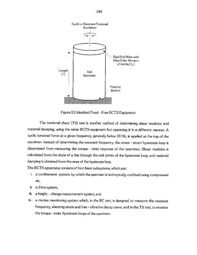
144
Cyclic or Resonant TorsionalExcitation
Rigid End Mass withMass Polar Moment
of Inertia [I0,]
Length Soil
[ I] Specimen
Fixed atBottom
Figure II.1 Idealized Fixed - Free RCTS Equipment
The torsional shear (TS) test -is another method of determining shear modulus and
material damping, using the same RCTS equipment but operating it in a different manner. A
cyclic torsional force at a given frequency, generally below 10 Hz, is applied at the top of the
specimen. Instead of determining the resonant frequency, the stress - strain hysteresis loop is
determined from measuring the torque - twist response of the specimen. Shear modulus is
calculated from the slope of a line through the end points of the hysteresis loop, and material
damping is obtained from the area of the hysteresis loop.
The RCTS apparatus consists of four basic subsystems, which are:
i. a confinement system, by which the specimen is isotropically confined using compressed
air,
ii. a drive system,
iii. a height - change measurement system, and
iv. a motion monitoring system which, in the RC test, is designed to measure the resonant
frequency, shearing strain and free - vibration decay curve, and in the TS test, to monitor
the torque - twist hysteresis loops of the specimen.
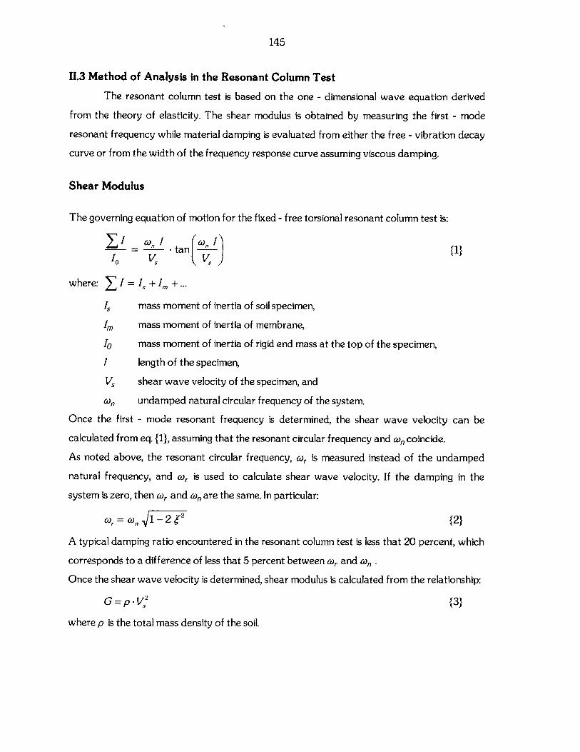
145
1.3 Method of Analysis in the Resonant Column Test
The resonant column test is based on the one - dimensional wave equation derived
from the theory of elasticity. The shear modulus is obtained by measuring the first - mode
resonant frequency while material damping is evaluated from either the free - vibration decay
curve or from the width of the frequency response curve assuming viscous damping.
Shear Modulus
The governing equation of motion for the fixed - free torsional resonant column test is:
I (0m, 1 0,/-= -- - tan ( {1}I0 V, V
where: Z/I,+IM,+...
I, mass moment of inertia of soil specimen,
Im mass moment of inertia of membrane,
I0 mass moment of inertia of rigid end mass at the top of the specimen,
I length of the specimen,
V, shear wave velocity of the specimen, and
on undamped natural circular frequency of the system.
Once the first - mode resonant frequency is determined, the shear wave velocity can be
calculated from eq. {1}, assuming that the resonant circular frequency and con coincide.
As noted above, the resonant circular frequency, o, is measured instead of the undamped
natural frequency, and cr is used to calculate shear wave velocity. If the damping in the
system is zero, then or and on are the same. In particular:
Or = 0), 1 - 2 2 2}
A typical damping ratio encountered in the resonant column test is less that 20 percent, which
corresponds to a difference of less that 5 percent between wr and con .
Once the shear wave velocity is determined, shear modulus is calculated from the relationship:
G=p -V 2 {3}
where p is the total mass density of the soil.
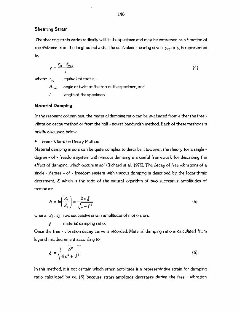
146
Shearing Strain
The shearing strain varies radically within the specimen and may be expressed as a function of
the distance from the longitudinal axis. The equivalent shearing strain, Yeq or y, is represented
by:
r-8y e= ' max {4}1
where: req equivalent radius,
,max angle of twist at the top of the specimen, and
/ length of the specimen.
Material Damping
In the resonant column test, the material damping ratio can be evaluated from either the free -
vibration decay method or from the half - power bandwidth method. Each of these methods is
briefly discussed below.
e Free - Vibration Decay Method
Material damping in soils can be quite complex to describe. However, the theory for a single -
degree - of - freedom system with viscous damping is a useful framework for describing the
effect of damping, which occurs in soil (Richard et al., 1970). The decay of free vibrations of a
single - degree - of - freedom system with viscous damping is described by the logarithmic
decrement, 6, which is the ratio of the natural logarithm of two successive amplitudes of
motion as:
6 ZI 2n(n {5}Z2 #
where: Z1, Z2 two successive strain amplitudes of motion, and
material damping ratio.
Once the free - vibration decay curve is recorded, Material damping ratio is calculated from
logarithmic decrement according to:
625 ={6}4ni2 +6 2
In this method, it is not certain which strain amplitude is a representative strain for damping
ratio calculated by eq. {6} because strain amplitude decreases during the free - vibration
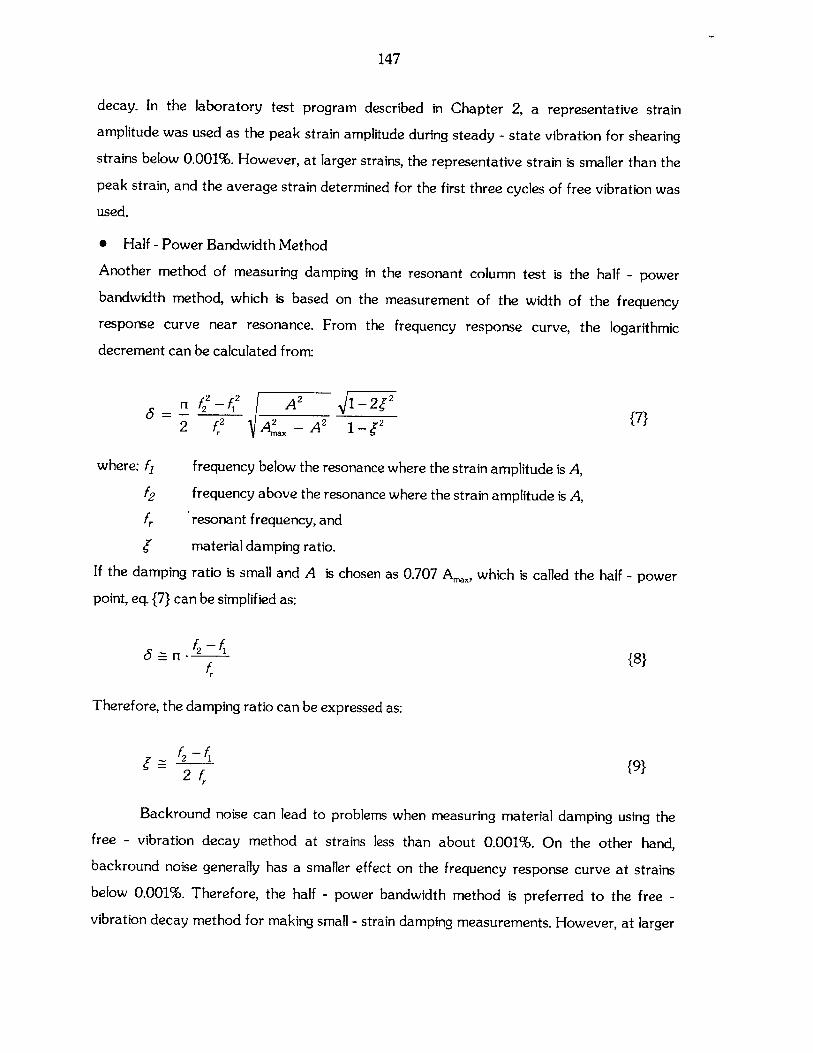
147
decay. In the laboratory test program described in Chapter 2, a representative strain
amplitude was used as the peak strain amplitude during steady - state vibration for shearing
strains below 0.001%. However, at larger strains, the representative strain is smaller than the
peak strain, and the average strain determined for the first three cycles of free vibration was
used.
* Half - Power Bandwidth Method
Another method of measuring damping in the resonant column test is the half - power
bandwidth method, which is based on the measurement of the width of the frequency
response curve near resonance. From the frequency response curve, the logarithmic
decrement can be calculated from:
f 2 fA -2(2(5 = -- - {7}f2 A - A 2 1-22 m ax
where: f, frequency below the resonance where the strain amplitude is A,f2 frequency above the resonance where the strain amplitude is A,
f,. 'resonant frequency, and
6 material damping ratio.
If the damping ratio is small and A is chosen as 0.707 Ax, which is called the half - power
point, eq. {7} can be simplified as:
f -f~ - 1 {8}
Therefore, the damping ratio can be expressed as:
f2 -f {9}
2 f,
Backround noise can lead to problems when measuring material damping using the
free - vibration decay method at strains less than about 0.001%. On the other hand,backround noise generally has a smaller effect on the frequency response curve at strains
below 0.001%. Therefore, the half - power bandwidth method is preferred to the free -
vibration decay method for making small - strain damping measurements. However, at larger
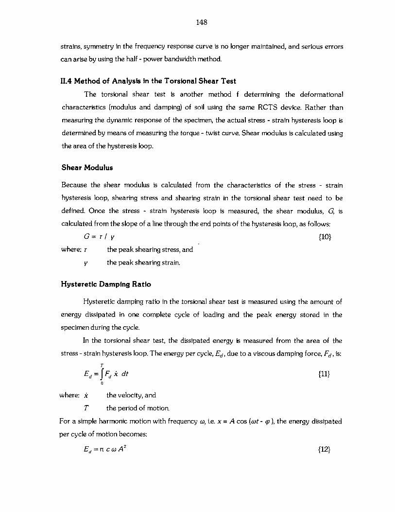
148
strains, symmetry in the frequency response curve is no longer maintained, and serious errors
can arise by using the half - power bandwidth method.
1.4 Method of Analysis in the Torsional Shear Test
The torsional shear test is another method f determining the deformational
characteristics (modulus and damping) of soil using the same RCTS device. Rather than
measuring the dynamic response of the specimen, the actual stress - strain hysteresis loop is
determined by means of measuring the torque - twist curve. Shear modulus is calculated using
the area of the hysteresis loop.
Shear Modulus
Because the shear modulus is calculated from the characteristics of the stress - strain
hysteresis loop, shearing stress and shearing strain in the torsional shear test need to be
defined. Once the stress - strain hysteresis loop is measured, the shear modulus, G, is
calculated from the slope of a line through the end points of the hysteresis loop, as follows:
G= rI y {10}
where: r the peak shearing stress, and
y the peak shearing strain.
Hysteretic Damping Ratio
Hysteretic damping ratio in the torsional shear test is measured using the amount of
energy dissipated in one complete cycle of loading and the peak energy stored in the
specimen during the cycle.
In the torsional shear test, the dissipated energy is measured from the area of the
stress - strain hysteresis loop. The energy per cycle, Ed, due to a viscous damping force, Fd, is:
T
Ed= Fd k dt {11}0
where: k the velocity, and
T the period of motion.
For a simple harmonic motion with frequency co, i.e. x = A cos (ot - p ), the energy dissipated
per cycle of motion becomes:
Ed = Ti c CO A 2 {12}
149
From eq. {12}, the viscous damping coefficient can be expressed as:
Wn (j2 A
The peak strain energy, W, stored by the spring is equal to the area under the secant modulus
line and can be written as:
W, = k A2 / 2 {14}
The critical damping coefficient, CC, is:
CC = 2- V km = 2 k / cn {15}
where k is an elastic spring constant, m is a mass, and con is a natural frequency of the system.
Using eq. {14}, eq. {15} can be rewritten as:
= ' W,{16}
and the damping ratio can be expressed as:
C W on {17)Cc 4 nW, w
For soils however, material damping is often assumed to be frequency indepednent.
Therefore, the term con 1o can be ignored, and hysteretic damping is written as:
1_ Wd {18}1r W~4 n W,
where: Wd the area of the hysteresis loop, and
W, the area under the secant modulus.
II.5 References
Chen, A. T. F., Stokoe, K. H., 11 (1979). "Interpretation of Strain Dependent Modulus andDamping from Torsional Soil Tests", Report No. USGS - GD - 79 - 002, NTIS NO. PB -298479, U.S. Geological Survey, 46 P.
Isenhower, W. M. (1979). "Torsional Simple Shear/Resonant Column Properties of SanFrancisco Bay Mud", MS. Thesis, GT 80-1, University of Texas at Austin, December, pp.307.
Kim, D.S. (1991). "Deformational Characteristics of Soils at Small to Intermediate Strains fromCyclic Tests", Ph.D. Dissertation, Geotechnical Engineering, Department of CivilEngineering, University of Texas at Austin, August.
150
Ni, S. H. (1987). "Dynamic Properties of Sand under True Triaxial Stress States fromResonant Column/Torsional Shear Tests", PhD. Dissertation, Geotechnical Engineering,Department of Civil Engineering, University of Texas at Austin, August.
Richard, F. E., Jr., Hall, J. R., Jr. and Woods, R. D. (1970). 'Vibrations of Soils and Foundations",Prentice Hal Inc., Englewood Cliffs, New Jersey, 414 p.
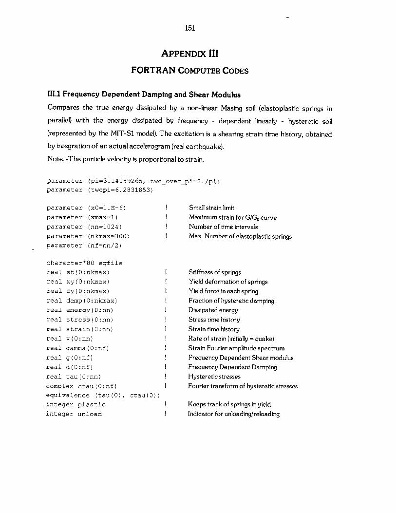
151
APPENDIX III
FORTRAN COMPUTER CODES
111.1 Frequency Dependent Damping and Shear Modulus
Compares the true energy dissipated by a non-linear Masing soil (elastoplastic springs in
parallel) with the energy dissipated by frequency - dependent linearly - hysteretic soil
(represented by the MIT-Si model). The excitation is a shearing strain time history, obtained
by integration of an actual accelerogram (real earthquake).
Note. -The particle velocity is proportional to strain.
parameter
parameter
parameter
parameter
parameter
parameter
parameter
(pi=3.14159265, two-overpi=2./pi)
(twopi=6.2831853)
(xO=1.E-6)
(xmax=1)
(nn=1024)
(nkmax=300)
(nf=nn/2)
Small strain limit
Maximum strain for G/Go curveNumber of time intervalsMax. Number of elastoplastic springs
character*80 eqfile
real st(O:nkmax)
real xy(O:nkmax)
real fy(O:nkmax)
real damp(O:nkmax)
real energy(O:nn)
real stress(O:nn)
real strain (0: nn)
real v(O:nn)
real gamma(O:nf)
real g(O:nf)
real d(O:nf)
real tau(O:nn)
complex ctau(O:nf)
equivalence (tau(O), ctau(O))
integer plastic
integer unload
Stiffness of springs
Yield deformation of springs
Yield force in each spring
Fraction of hysteretic damping
Dissipated energy
Stress time history
Strain time history
Rate of strain (initially = quake)
Strain Fourier amplitude spectrum
Frequency Dependent Shear modulus
Frequency Dependent Damping
Hysteretic stresses
Fourier transform of hysteretic stresses
Keeps track of springs in yield
Indicator for unloading/reloading
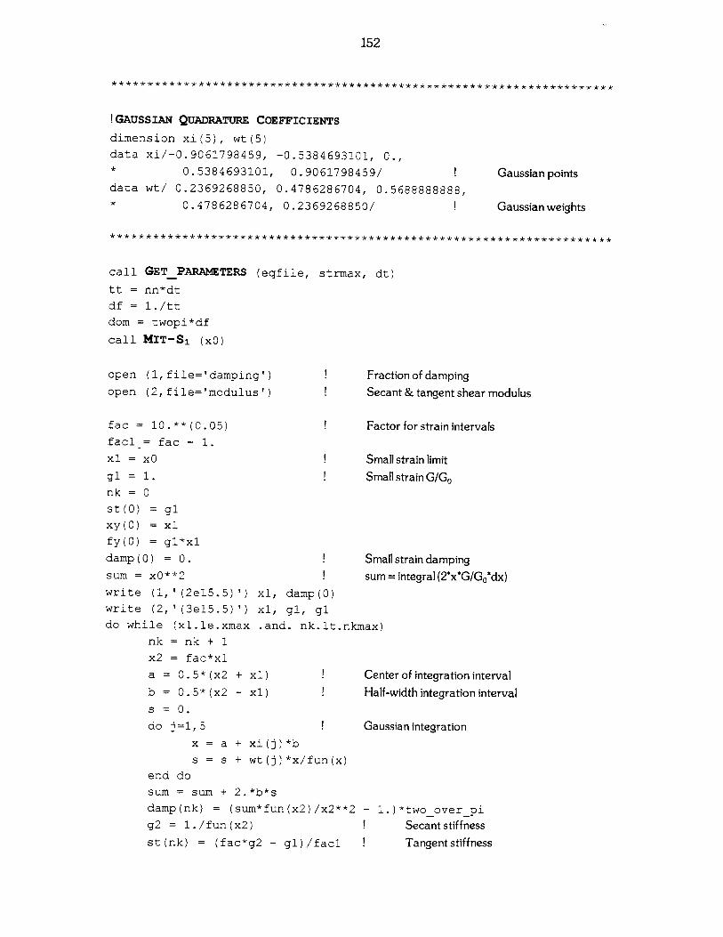
152
***************************************************** *********** ****
!GAUSSIAN QUADRATURE COEFFICIENTS
dimension xi(5), wt(5)
data xi/-0.9061798459, -0.5384693101, 0.,
* 0.5384693101, 0.9061798459/
data wt/ 0.2369268850, 0.4786286704, 0.5688888888,* 0.4786286704, 0.2369268850/
call GETPARAMETERS (eqfile, strma
tt = nn*dt
df = 1./tt
dom = twopi*df
call MIT-Si (xO)
open (1,file='damping')
open (2,file='modulus')
fac = 10.**(0.05)
fac1 = fac - 1.
x1 = x0
gl = 1.nk = 0
st(0) = gl
xy(0) = x1
fy(0) = gl*xl
damp(0) = 0.
sum = xO**2
write (1,'(2e15.5)') x1, damp(0)
write (2,'(3e15.5)') x1, gl, gl
do while (xl.le.xmax .and. nk.lt.nk
nk = nk + 1
x2 = fac*xl
a = 0.5*(x2 + xl)
b = 0.5*(x2 - xl)
s = 0.
do j=1,5
x = a + xi(j)*b
s = s + wt(j)*x/fun(x)
end do
sum = sum + 2.*b*s
damp(nk) = (sum*fun(x2)/x2**2
g2 = 1./fun(x2)
st(nk) = (fac*g2 - gl)/facl
x, dt)
Fraction of dampingSecant & tangent shear modulus
Factor for strain intervals
Small strain limitSmall strain G/Go
Small strain dampingsum = integral (2*x*G/Go*dx)
max)
Center of integration intervalHalf-width integration interval
Gaussian integration
- 1.)*two over pi
Secant stiffnessTangent stiffness
Gaussian points
Gaussian weights
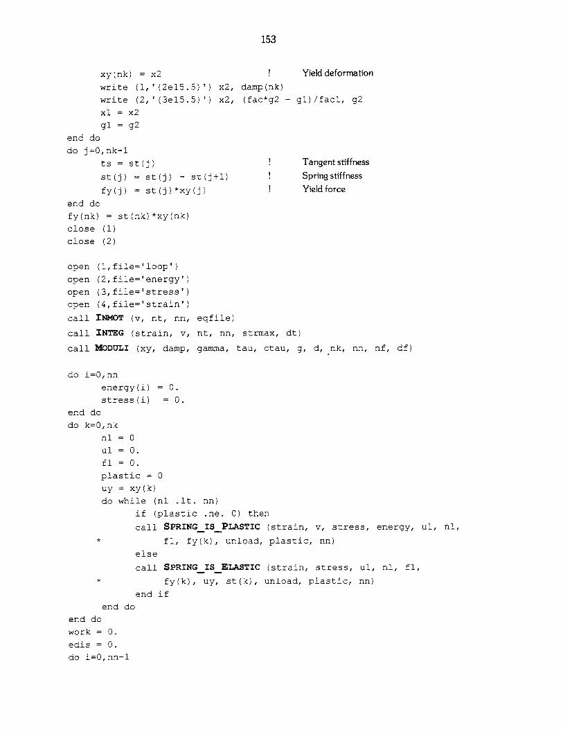
153
xy (nk) = x2 Yield deformation
write (1,'(2e15.5)') x2, damp(nk)
write (2,' (3e15.5) ') x2, (fac*g2 - gl)/facl, g2x1 = x2
gl = g2
end do
do j=O,nk-1
ts = st (j) Tangent stiffness
st (j) = st (j) - st (j+1) Spring stiffness
fy(j) = st(j)*xy(j) Yield force
end do
fy(nk) = st(nk)*xy(nk)
close (1)
close (2)
open (l,file='loop')
open (2,file='energy')
open (3,file='stress')
open (4,file='strain')
call INMOT (v, nt, nn, eqfile)
call INTEG (strain, v, nt, nn, strmax, dt)
call MODULI (xy, damp, gamma, tau, ctau, g, d, nk, nn, nf, df)
do i=O,nn
energy(i) 0.
stress(i) = 0.
end do
do k=0,nk
nl = 0
ul = 0.
fl = 0.
plastic = 0
uy = xy(k)
do while (nl .lt. nn)
if (plastic .ne. 0) then
call SPRING IS PLASTIC (strain, v, stress, energy, ul, n1,
* fl, fy(k), unload, plastic, nn)
else
call SPRING ISELASTIC (strain, stress, ul, nl, fl,
* fy(k), uy, st(k), unload, plastic, nn)
end if
end do
end do
work = 0.
edis = 0.
do i=0,nn-1
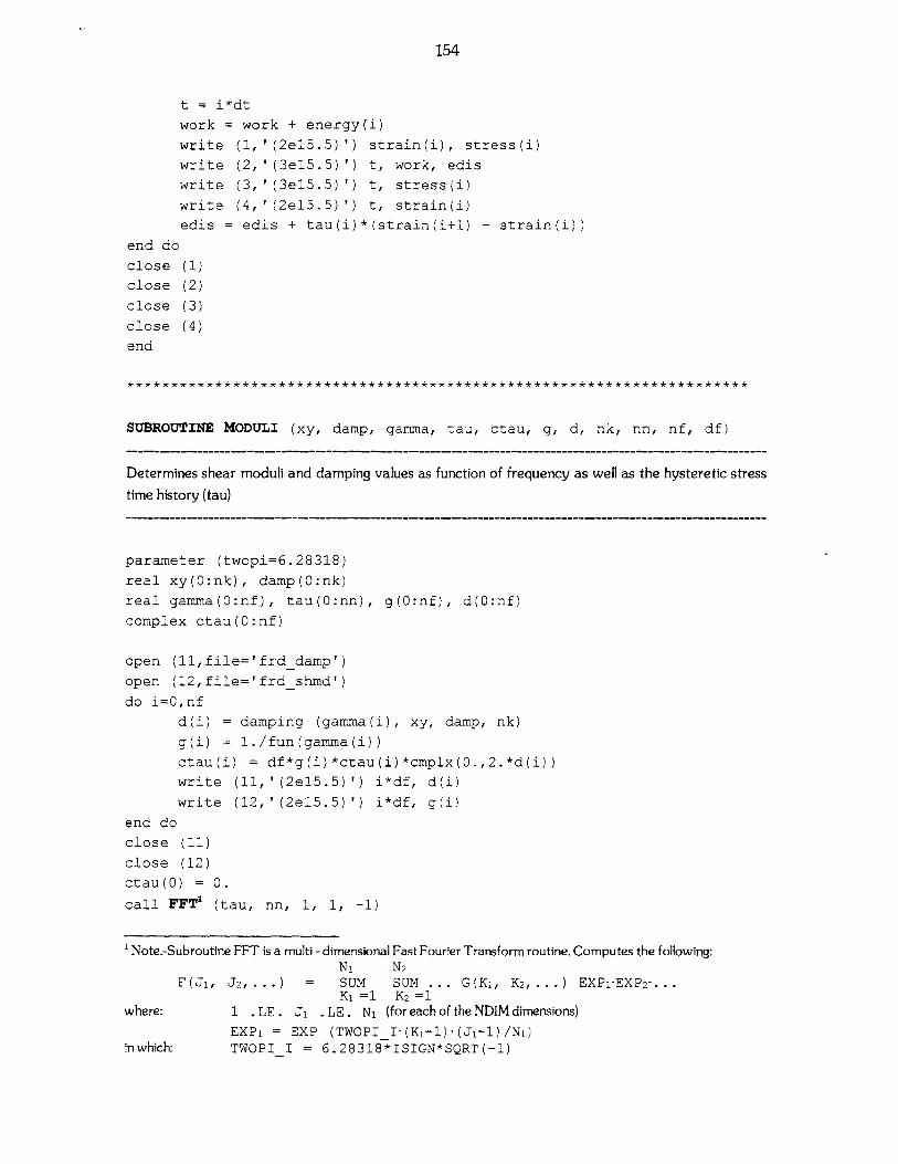
154
t = i*dt
work = work + energy
write (l,'(2e15.5)')
write (2,'(3e15.5)')
write (3,'(3e15.5)')
write (4,'(2e15.5)')
edis = edis + tau(i)
(i)
strain(i), stress(i)t, work, edis
t, stress(i)
t, strain(i)
*(strain(i+1) - strain(i))
(1)(2)
(3)(4)
SUBROUTINE MODULI (xy, damp, gamma, tau, ctau, g, d, nk, nn, nf, df)
Determines shear moduli and damping values as function of frequency as well as the hysteretic stress
time history (tau)
parameter (twopi=6.28318)
real xy(O:nk), damp(O:nk)
real gamma(O:nf), tau(O:nn),
complex ctau(0:nf)
g(0:nf), d(0:nf)
open (11,file='frddamp')
open (12,file='frd_shmd')
do i=0,nf
d (i) = damping (gamma (i) , xy, damp, nk)
g(i) = l./fun(gamma(i))
ctau(i) = df*g(i)*ctau(i)*cmplx(0.,2.*d(i))
write (11,'(2e15.5)') i*df, d(i)
write (12,'(2e15.5)') i*df, g(i)
end do
close (11)
close (12)
ctau(0) = 0.
call FFT' (tau, nn, 1, 1, -1)
Note.-Subroutine FFT is a multi - dimensional Fast Fourier Transform routine. Computes the following:Ni N2
F (Ji , J 2 ,...) = SUM SUM ... G(Ki, K2,...) EXPr EXP 2-..-Ki =1 K 2 =1
where: 1 . LE. J. LE. Ni (for each of the NDIM dimensions)
EXPi = EXP (TWOPII- (Ki-1) - (Ji-1) /N1 )inwhich: TWOPII = 6.28318*ISIGN*SQRT(-1)
end do
close
close
close
close
end
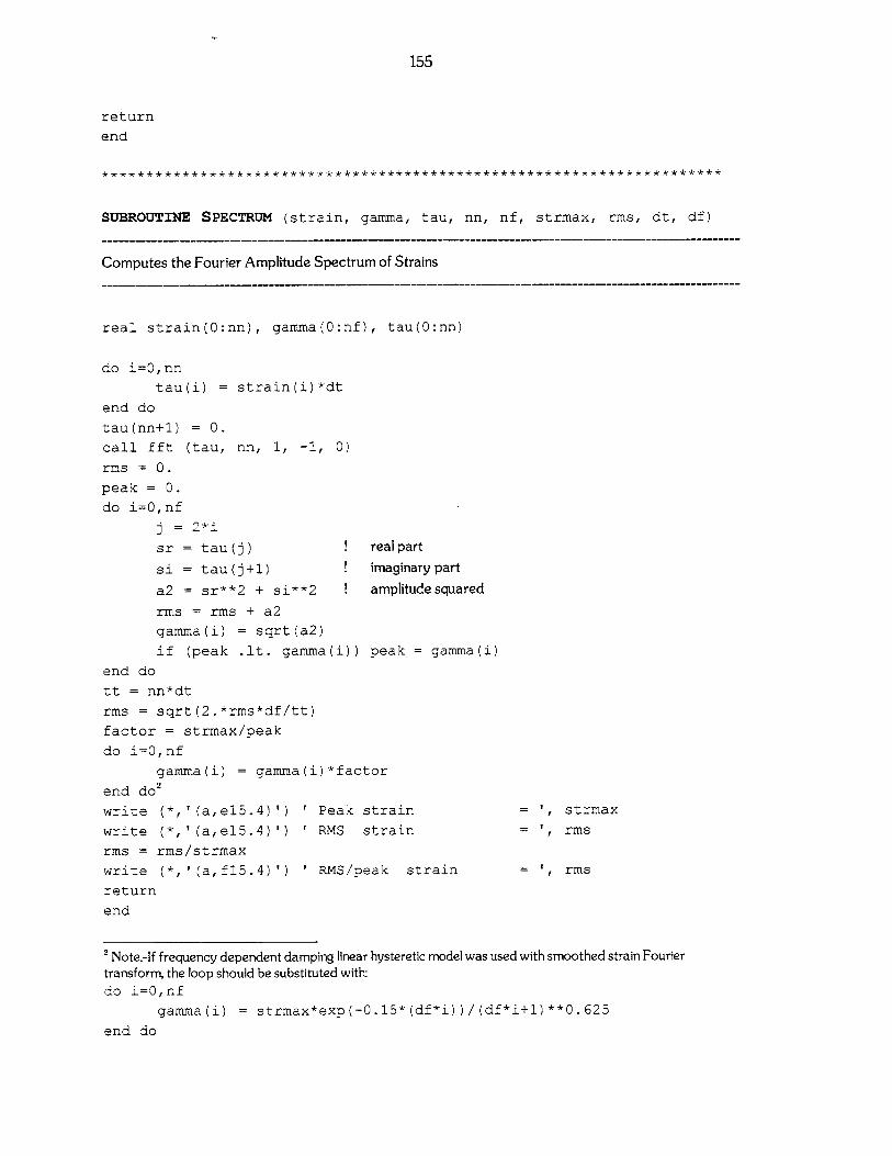
155
return
end
SUBROUTINE SPECTRUM (strain, gamma, tau, nn, nf, strmax, rms, dt, df)
Computes the Fourier Amplitude Spectrum of Strains
real strain(O:nn), gamma(O:nf), tau(O:nn)
do i=O, nn
tau(i) = strain(i)*dt
end do
tau(nn+1) = 0.
call fft (tau, nn, 1, -1, 0)
rms = 0.
peak = 0.
do i=0,nf
j = 2*i
sr = tau(j) ! realpart
si = tau(j+1) ! imaginary part
a2 sr**2 + si**2 ! amplitude squared
rms rms + a2
gamma(i) = sqrt(a2)
if (peak .lt. gamma (i)) peak = gamma (i)
end do
tt = nn*dt
rms = sqrt(2.*rms*df/tt)
factor = strmax/peak
do i=0,nf
gamma(i) = gamma(i)*factor
end do2
write (*,'(a,e15.4)') ' Peak strain
write (*,'(a,e15.4)') ' RMS strain
rms = rms/strmax
write (*,'(a, f15. 4)') ' RMS/peak strain
return
end
= ', strmax
= ', rms
= ', rms
2 Note.-If frequency dependent damping linear hysteretic model was used with smoothed strain Fouriertransform, the loop should be substituted with:do i=0,nf
gamma(i) = strmax*exp(-0.15*(df*i))/(df*i+1)**0.625
end do
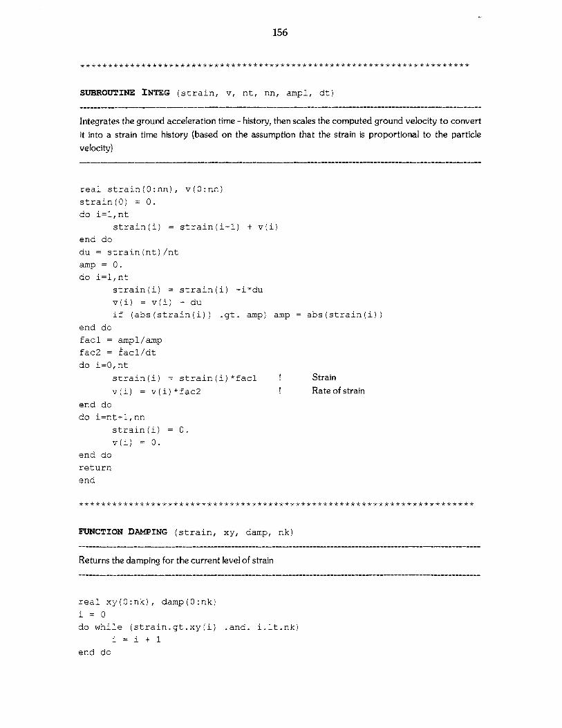
156
SUBROUTINE INTEG (strain, v, nt, nn, ampl, dt)
Integrates the ground acceleration time - history, then scales the computed ground velocity to convert
it into a strain time history (based on the assumption that the strain is proportional to the particle
velocity)
real strain(O:nn), v(O:nn)
strain(O) = 0.
do i=1,nt
strain(i) = strain(i-1) + v(i)
end do
du = strain(nt)/nt
amp = 0.
do i=1,nt
strain(i) = strain(i) -i*du
v(i) = v(i) - du
if (abs(strain(i)) .gt. amp) amp abs(strain(i))
end do
fac1 = ampl/amp
fac2 = facl/dt
do i=0,nt
strain(i) = strain(i)*facl ! Strain
v(i) = v(i)*fac2 Rate of strain
end do
do i=nt+1,nn
strain(i) = 0.
v(i) = 0.
end do
return
end
FUNCTION DAMPING (strain, xy, damp, nk)
Returns the damping for the current level of strain
real xy(0:nk), damp(0:nk)
i = 0
do while (strain.gt.xy(i) .and. i.lt.nk)
i =i + 1
end do
157
if (i .le. 1) then
damping = damp(l)*strain/xy(l)
else if (strain .le. xy(nk)) then
dd = log( xy(i)/xy(i-1)
xl = log( xy(i)/strain
x2 = log( strain/xy(i-1))
damping = (xl*damp(i-1) + x2*damp(i))/dd
else
damping = damp (nk)
end if
return
end
Must modify for strain > xy(nk)
**************** ************* ************************** **** **** *** ****
SUBROUTINE GETPARAMETERS (inpfil, strmax, dt)
Returns the parameters on the command line
character*80 inpfil
character*5 type
real KO
integer*2 status
common /soil/ Cb, eO,
! *** Default values
e0 = 0.5
KO = 0.5
conf = 1.
type = 'sand'
strmax = 1.e-3
dt = 0.02
n = nargs ()if (n .ge. 2) then
call GETARG (1,
else
KO, conf, xmin
Void ratio
Coefficient of lateral earth pressure
Atmospheres
Maximum strain
Time step for earthquake
inpfile, status) ! Get name from command line
write (*,'(a)') ' Input file?'
read (*,'(a)') inpfile
end if
open (5,file=inpfil)
read (5,'(a)') type
read (5,*) eO
read (5,*) KO
158
read (5,*) conf
read (5,'(a)') inpfil
read (5,*) dt
read (5,*) strmax
close (5)
if (type.eq.'clay' .or. type.eq.'CLAY') then
Cb = 450.
else
Cb = 800
end if
return
end
SUBROUTINE MIT-Si (xO)
Computes the soil constants for the MIT - S1 model shear modulus degradation curves
real KO, KONC
parameter (FTHRD=1.6666667, TWOTHRD=0.6666667)
parameter (SR15=1.224744871) sqrt(1.5)
parameter (OCR1=6.67777) OCRatKo=1
parameter (POISO=0 .25) Small Strain Poisson's ratio
parameter (KONC=0.5)
common /soil/ Cb, eO, KO, conf, xmin
common /constants/ C, C1, C2, C12, C3, C4, Al, A2, B1, B2, B3, GO
conf = (1.+2.*KO)*conf/3.
e = e0*exp(-0.00169*conf) Voidratio
Cl = 2.4 Exper. Data (Laird & Stokoe, 1993)
C = (1. - 2.*POISO)/(l. + POISO)C2 = c*(1 + 2.*KONC - 3./OCR1)
C2 = SR15*(KONC - 1. + C2)*(l.+ 2*KONC)/(l.- KONC)**2
C = e*conf**TWOTHRD/( 1.5*C*Cb*(l. + e)C11 = C1**2
C12 = C1*C2
C22 = C2**2
Al = 12.*C12**2
A2 = C*(Cl + C2)*(4.*C12 - Cll - C22)
Bl = 3.*Al
B2 = 6.*A2
B3 = (10.*C12 - 3.*(Cll + C22))*C**2C12 = 2.*C12
C3 = (Cl - C2)**2
159
C4 = C1 + C2
GO = 1.
GO = l./fun(xO)
xmin = xO
return
end
Set appropriate value before calling FUN ( )
FUNCTION FUN(xO)
Shear modulus degradation curve
parameter (THIRD=0.3333333)
common /soil/ Cb, eO, KO, conf, xmin
common /constants/ C, C1, C2, C12, C3, C4, Al, A2, B1, B2, B3, GO
if (x .le. xmin) then
FUN 1.
else
A = Al*x + A2
B = C12*sqrt((Bl*x + B2)*x + B3)
A = ((A + B)/C)**THIRD
T = conf*(A + C3/A - C4)/C12
G = T/x
FUN = GO/G
end if
return
end
Stressat strain = xShear modulus
************************************************************* **********
SUBROUTINE SPRINGISPLASTIC (u, v, stress, energy, ul, n1, f 1,
* fy, unload, plastic, nt)
Determines the point at which the spring will stop flowing as well as the energy dissipated by it in plastic
flow
real u(0:nt), v(0:nt), stress(0:nt), energy(0:nt)
n2 = n1
if (plastic .eq. 1) then
do while (v(n2) .ge.0. .and. n2.It.nt)
n2 = n2 + 1
end do
Flowing L->R
160
unload = -1
f2 = fy
else if (plastic .eq. -1) then
do while (v(n2).le.0. .and. n2.lt.nt)
n2 = n2 + 1
end do
unload =
f2 = -fy
1
end if
plastic = 0
n2 = n2 - 1
u2 = u(n2)
work = (u2 - ul)*f2
if (n2 .gt. n1) then
work = work/ (n2 - n1)
energy(nl) = energy(n1) + 0.5*work
energy(n2) = energy(n2) + 0.5*work
do i=nl+1,n2-1
energy(i) = energy(i) + work
end do
else
energy(n2) = energy(n2) + work
end if
do i=nl+1, n2
stress(i) = stress(i) + f2
end do
fl = f2
ul = u2
nl = n2
return
end
SUBROUTINE SPRINGIS_ELASTIC (u, stress, ul, n1, fl, fy, uy,
* st, unload, plastic, nt)
Determines the next point at which spring will flow (if at all)
real u(O:nt), stress(O:nt)
integer unload, plastic
n2 = nl + 1
if (unload .lt. 0) then Springunloading?
u2 = ul - uy Yes. Set lower yield limit
do while (u(n2).lt.ul .and. u(n2).gt.u2 .and. n2.lt.nt)
n2 = n2 + 1
Flowing R->L
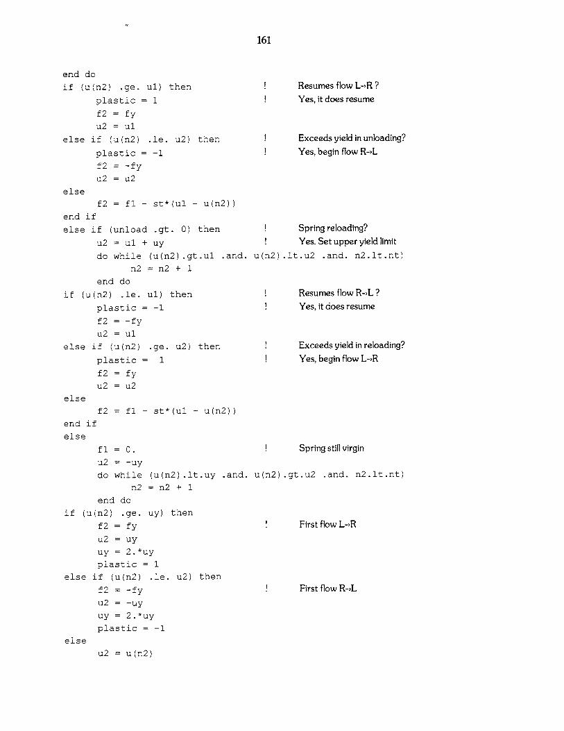
161
end do
if (u(n2) .ge. ul) then
plastic = 1
f2 = fy
u2 = ul
else if (u(n2) .le. u2) then
plastic = -1
f2 = -fy
u2 = u2
else
f2 = f1 - st*(ul - u(n2))
end if
else if (unload .gt. 0) then
u2 = ul + uy
do while (u(n2).gt.ul .and. u
n2 = n2 + 1
end do
if (u(n2) .le. ul) then
plastic = -1
f2 = -fy
u2 = ul
else if (u(n2) .ge. u2) then
plastic = 1
f2 = fy
u2 = u2
else
ff2 = f1 - st*(ul - u(n2))
end if
else
Resumes flow L->R ?
Yes, it does resume
Exceeds yield in unloading?
Yes, begin flow R->L
(n2)
Spring reloading?Yes. Set upper yield limit
.lt.u2 .and. n2.lt.nt)
Resumes flow R->L?Yes, it does resume
Exceeds yield in reloading?
Yes, begin flow L->R
f1 = 0. Spring still virgin
u2 = -uy
do while (u(n2).lt.uy .and. u(n2).gt.u2 .and. n2.lt.nt)
n2 = n2 + 1
end do
if (u(n2) .ge. uy) then
f2 = fy
u2 = uy
uy = 2.*uy
plastic = 1
else if (u(n2) .le. u2) then
ff2 = -fy
u2 = -uy
uy = 2.*uy
plastic = -1
else
u2 = u(n2)
First flow L->R
First flow R->L
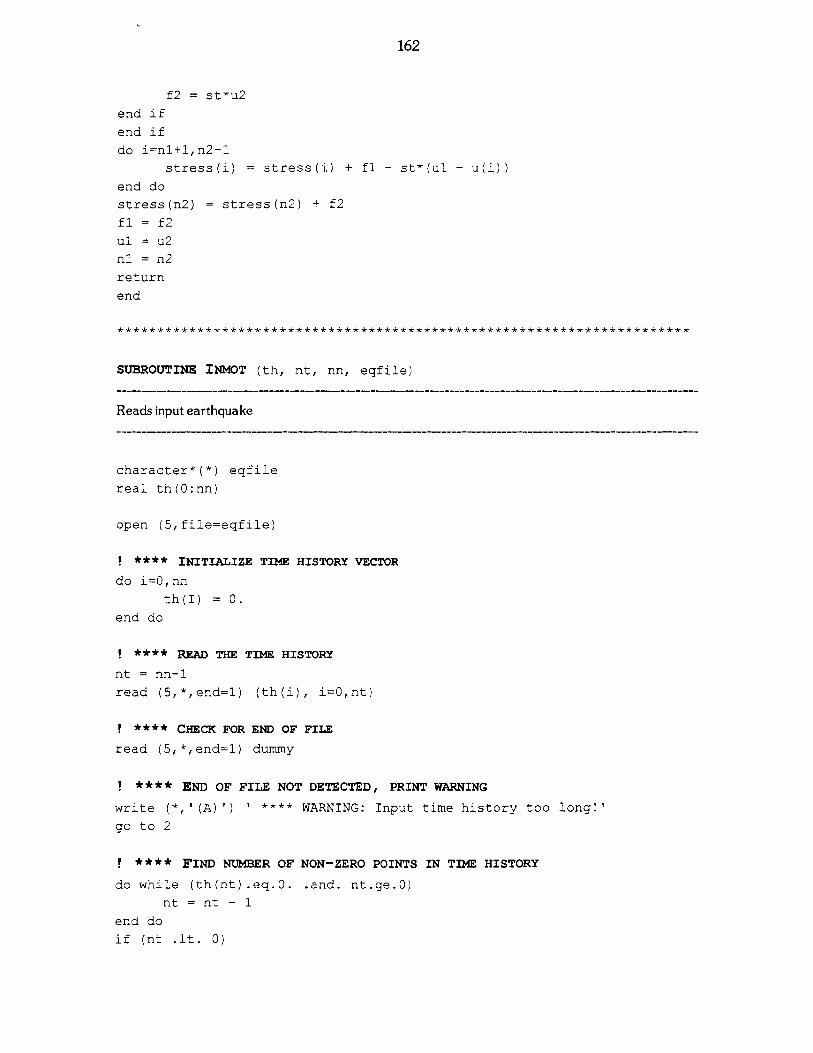
162
f2 = st*u2
end if
end if
do i=nl+1,n2-1
stress(i) = stress(i) + f1 - st*(ul - u(i))
end do
stress(n2) = stress(n2) + f2
fl = f2
ul = u2n1 = n2
return
end
******************* ******************************* ******** *************
SUBROUTINE INMOT (th, nt, nn, eqfile)
Reads input earthquake
character*(*) eqfile
real th(O:nn)
open (5,file=eqfile)
I **** INITIALIZE TIME HISTORY VECTOR
do i=O,nn
th(I) = 0.
end do
I **** READ THE TIME HISTORY
nt = nn-1
read (5,*,end=1) (th(i), i=0,nt)
! **** CHECK FOR END OF FILE
read (5,*,end=l) dummy
! **** END OF FILE NOT DETECTED, PRINT WARNING
write (*, ' (A)') ' * WARNING: Input time history too long!
go to 2
1 **** FIND NUMBER OF NON-ZERO POINTS IN TIME HISTORY
do while (th(nt).eq.0. .and. nt.ge.0)
nt = nt - 1
end do
if (nt .lt. 0)

163
*
close (5)
return
end
stop ' **** ERROR: Input time history is empty!'
************** ******************* **************************************
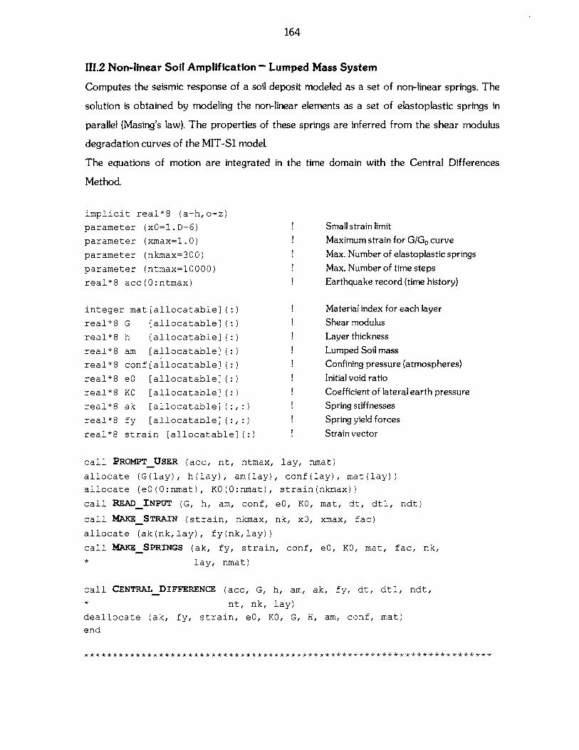
164
111.2 Non-linear Soil Amplification - Lumped Mass System
Computes the seismic response of a soil deposit modeled as a set of non-linear springs. The
solution is obtained by modeling the non-linear elements as a set of elastoplastic springs in
parallel (Masing's law). The properties of these springs are inferred from the shear modulus
degradation curves of the MIT-Si model.
The equations of motion are integrated in the time domain with the Central Differences
Method.
implicit real*8 (a-h,o-z)
parameter (x0=1.D-6)
parameter (xmax=1 .0)
parameter (nkmax=300)
parameter (ntmax=10000)
real*8 acc(O:ntmax)
integer mat [allocatable] (:)
G
h
am
conf
eO
KO
ak
fy
real*8 strain
[allocatable]
[allocatable]
[allocatable]
[allocatable]
[allocatable]
[allocat able]
[allocatable]
[allocatable]
[allocatable] ( :)
Small strain limit
Maximum strain for G/Go curve
Max. Number of elastoplastic springs
Max. Number of time steps
Earthquake record (time history)
Material index for each layer
Shear modulus
Layer thickness
Lumped Soil mass
Confining pressure (atmospheres)
Initial void ratio
Coefficient of lateral earth pressure
Spring stiffnesses
Spring yield forces
Strain vector
call PROMPTUSER (acc, nt, ntmax, lay, nmat)
allocate (G(lay), h(lay), am(lay), conf(lay), mat(lay))
allocate (eO(0:nmat), KO(0:nmat), strain(nkmax))
call READINPUT (G, h, am, conf, eG, KO, mat, dt, dtl, ndt)
call MAKESTRAIN (strain, nkmax, nk, xO, xmax, fac)
allocate (ak(nk,lay), fy(nk,lay))
call MAKESPRINGS (ak, fy, strain, conf, eO, KO, mat, fac, nk,
* lay, nmat)
call CENTRAL DIFFERENCE (acc, G, h, am, ak, fy, dt, dtl, ndt,
* nt, nk, lay)
deallocate (ak, fy, strain, eO, KO, G, H, am, conf, mat)
end
real*8
real*8
real*8
real*8
real*8
real*8
real*8
real*8
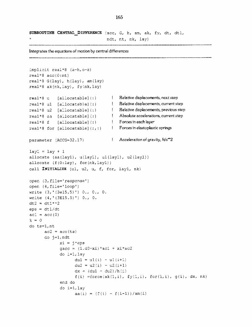
165
SUBROUTINE CENTRALDIFFERENCE (acc, G, h, am, ak, fy, dt, dtl,
* ndt, nt, nk, lay)
Integrates the equations of motion by central differences
implicit real*8 (a-h,o-z)
real*8 acc(O:nt)
real*8 G(lay), h(lay), am(lay)
real*8 ak(nk,lay), fy(nk,lay)
U
ul
u2
aa
f
for
[allocatable]
[allocatable]
[allocatable]
[allocatable]
[allocatable]
[allocat able]
parameter (ACCG=32. 17)
layl = lay + 1
allocate (aa(layl),
allocate (f(O:lay),
call INITIALIZE (ul,
u (layl)
for (nk,
u2, u,
Relative displacements, next step
Relative displacements, current step
Relative displacements, previous step
Absolute accelerations, current stepForces in each layer
Forces in elastoplastic springs
Acceleration of gravity, ft/s**2
, ul(layl), u2(lay2))
layl))
f, for, layl, nk)
open (3,file='response')
open (4,file='loop')
write (3,'(3e15.5)') 0., 0., 0.
write (4,'(3E15.5)') 0., 0.
dt2 = dtl**2
eps = dtl/dt
acl = acc(0)
k= 0
do ts=1,nt
ac2 = acc(ts)
do j=1,ndt
xi = j*eps
gacc = (1.d0-xi)*ac1 + xi*ac2
do i=1,lay
dul = ul(i) - ul(i+1)
du2 = u2(i) - u2(i+1)
dx = (dul - du2)/h(i)
f(i) =force(ak(1,i), fy(1,i),
end do
do i=1,lay
aa(i) = (f(i) - f(i-1))/am(i)
for(1,i), g(i), dx, nk)
real*8
real*8
real*8
real*8
real*8
real*8
166
u(i) = 2.*ul(i) - u2(i) - dt2*(gacc + aa(i))u2(i) = ul(i)
ul(i) = u(i)
end do
k = k + 1
time = k*dtl
write (3,'(3E15.5)') time, -aa(1)/ACCG, gacc/ACCG
write (4,'(3E15.5)') ul(1), f(1)
end do
acl = ac2
end do
deallocate (aa, u, ul, u2, f, for)
close (3)
close (4)
return
end
************************************************************ **** *******
REAL*8 FUNCTION FORCE (ak, fy, for, G, dx, nk)
Computes the non-linear force in current layer
implicit real*8 (a-h,o-z)
dimension ak(*), fy(*), for(*)
force = 0.
do i=1,nk
for(i) = for(i) + ak(i)*dx
if (for(i) .gt. fy(i)) then
for(i) = fy(i)
else if (for(i) .lt. -fy(I)) then
for(i) = -fy(i)
end if
force = force + for(i)
end do
force = g*force
return
end
167
REAL*8 FUNCTION FUN (x)
Shear modulus degradation curve
implicit real*8 (a-h,o-z)parameter (THIRD=0.333333333333333DO)
common /soil/ Cb, conf
common /constants/ C, Cl, C2, C12, C3, C4, Al, A2, B1, B2, B3, GO
A = Al*x + A2
B = C12*sqrt((Bl*x + B2)*x + B3)
A = ((A + B)/C)**THIRD
T = conf*(A + C3/A - C4)/C12
G = T/x
FUN = GO/G
return
end
Stress at strain = xShear modulus
SUBROUTINE INITIALIZE (ul, u2, u, f, for, layl, nk)
Initializes the arrays
implicit real*8 (a-h,o-z)
real*8 ul(*), u2(*), u(*), f(*)
real*8 for(nk,layl)
do i=l,layldo j=1,nk
for(j,i) = 0.
end doul(I) = 0.
u2(I) = 0.
u(I) = 0.
f(I) = 0.
end do
returnend
168
SUBROUTINE MAKESTRAIN (strain, nkmax, nk, xO, xmax, fac)
Generates the strain vector
implicit real*8 (a-h,o-z)
real*8 strain (nkmax)
fac = 10.**(0.05) ! Factor forstrainintervals
strain (1) =x ! Small strain limit
nk = 1
x1 = x0
do while (xl.le.xmax .and. nk.lt.nkmax)
nk = nk + 1
x1 = fac*xl
strain(nk) = xl
end do
return
end
SUBROUTINE MAKESPRINGS (ak, fy, strain, conf, eO, KO, mat,
* fac, nk, lay, nmat)
Computes the elasto-plastic springs for current soil
implicit real*8 (a-h,o-z)
real*8 ak(nk,lay), fy(nk,lay), strain(nk)
real*8 conf(lay), eO(0:nmat), KO(0:nmat)
integer mat (nmat)
fac = fac - 1.
nkl = nk - 1
do i=l,lay
m = mat(i)
call MIT_S1 (strain(l), conf(i), eO(m), KO(m))
gl = 1. Small strain G/Go
fy(l,i) = gl*strain(l)
ak(l,i) = gl
do j=2,nk
x2 = strain(j)
g2 = 1. / fun (x2) Secant stiffness
ak(j,i) = (fac*g2 - gl)/facl ! Tangent stiffness
gl = g2
169
end do
do j=l,nkl
ak(j,i) = ak(j,i) - ak(j+l,i)
fy(j,i) = ak(j,i)*strain(j)
end do
fy(nk,i) = ak(nk,i)*strain(nk)
end do
return
end
Spring stiffnessYield force
SUBROUTINE MIT-Si (xO, sconf, eO, KO)
Computes the soil constants for the MIT - S1 model shear modulus degradation curves
real KO, KONC
parameter (FTHRD=1.6666667, TWOTHRD=0.6666667)
parameter (SR15=1.224744871) sqrt(1.5)
parameter (OCR1=6.67777) OCR at Ko=1
parameter (POISO=0 .25) Small Strain Poisson's ratio
parameter (KONC=0.5)
common /soil/ Cb, eO, KO, conf, xmin
common /constants/ C, Cl, C2, C12, C3, C4, Al, A2, B1, B2, B3, GO
! DEFAULT VALUES
Cb = 800. Sand (for Clay, use Cb = 450.)
! DEFINE CONSTANTS
conf = (1.+2.*KO)*sconf/3.
e = e0*exp(-0.00169*conf) Voidratio
C1 = 2.4 Exper. Data (Laird & Stokoe, 1993)
C = (1. - 2.*POISO)/(l. + POISO)
C2 = c*(l + 2.*KONC - 3./OCR1)
C2 = SR15*(KONC - 1. + C2)*(1.+ 2*KONC)/(l.- KONC)**2
C = e*conf**TWOTHRD/( 1.5*C*Cb*(l. + e)
C11 = C1**2
C12 = C1*C2
C22 = C2**2
Al = 12.*C12**2
A2 = C*(Cl + C2)*(4.*C12 - C11 - C22)
B1 = 3.*A1
B2 = 6.*A2
B3 = (10.*C12 - 3.*(C11 + C22))*C**2
170
C12 = 2.*C12
C3 = (Cl - C2)**2
C4 = C1 + C2
GO = 1. Set appropriate value before calling FUN ()
GO 1./fun(xO)
return
end
*************** ********************************************************
SUBROUTINE PROMPTUSER (acc, nt, ntmax, lay, nmat)
Returns the parameters on the command line, or prompts the user
implicit real*8 (a-h,o-z)
integer*2 status
real*8 acc(*)
character*80 input, quake, output
n = nargs ()
if (n .ge. 4) then
! ** GET FILE NAMES FROM COMMAND LINE
call GETARG (1, input, status)
call GETARG (2, quake, status)
call GETARG (3, output, status)
else
write (*,'(a)') ' Input data file?
read (*,'(a)') input
write (*,'(a)) ' Earthquake file?'
read (*,'(a)') quake
write (*,'(a)') ' Output file?
read (*,'(a)') output
end if
open (1,file=input, status='old')
open (2,file=quake, status='old')
call SCANINPUT (lay, nmat, scale)
call READQUAKE (acc, scale, nt, ntmax, 2)
close (2)
open (2,file=output)
return
end
171
SUBROUTINE READQUAKE (th, scale, nt, nn, unit)
Reads - Scales input earthquake
implicit real*8 (a-h,o-z)
integer unit
real*8 th(O:nn)
character*1 marker
character*80 row
parameter (ACCG=32 . 17) Acceleration of gravity, ft/s**2
marker = ' '
do while (marker.ne.';' .and. marker.ne.'/')
read (unit,'(al)', end=l) marker
enddo
if (marker .eq. '/') then
do while (marker .eq. '/')
read (unit,'(al)') marker
enddo
backspace (unit)
endif
go to 2
1 write (*,'(a)')
* ' Could not find marker in earthquake. Will try without...'
rewind (unit)
2 read (unit, '(a)') row Read first line of quake...
backspace (unit) ... and return to previous line
nl = 0
i= 80
do while (i .gt. 0) Find number of items in line
do while (row(i:i).eq.' ' .and. i.gt.0) !Jump over white
i = i - 1
enddo
if (i .gt. 0) then
nl = nl + 1
do while (row(i:i).ne.' ' .and. i.gt.0)
i=i- 1
enddo
endif
enddo
! *** INITIALIZE TINE HISTORY FILE
do i=0,nn
th(i) = 0.
enddo
! Jump over number
Find marker
Skip over remaining Ps
172
if (nl .gt. 4) then
* *** READ NORMAL EARTHQUAKE FILE
nil = nl - 1
do nt=O,nn-nll,nl
read (unit,*,err=3,end=3) (th(i), i=nt,nt+nll)
enddo
else if (nl .eq. 1) then
! * READ A SINGLE COLUMN OF ACCELERATION VALUES
do nt=O,nn
read (unit,*,err=3,end=3) th(nt)
enddo
else
* READ A "Time history" FILE (TIME, ACC, VEL, DISP)
do nt=O,nn
read (unit,*,err=3,end=3) t, th(nt)
enddo
endif
3 nt = nn
do while (nt.ge.O ~.and. th(nt) .eq.0.)
nt = nt - 1
enddo
if (nt .lt. 0)
* stop ' **** ERROR: Input time history is empty!'
** SCALE THE "Time history" FILE
call GETMAX(nt, NMAX, dt, TMAX, ATHMAX, THMAX, th)
if (scale .EQ. 0.) scale = ATHMAX
FACTOR = scale/ATHMAX
do i=0,nt
th(i) = th(i)*FACTOR*ACCG
end do
return
end
173
SUBROUTINE GETMAX (NEQ, NMAX, DT, TMAX, ATHMAX, THMAX, TH)
Finds the signed and absolute maxima of the array TH, ie. THMAX = TH (NMAX), and ATHMAX=ABS (THMAX) where NMAX is the corresponding index, and TMAX the time of max.
integer neq, nmaxreal*8 dt, tmax, athmax, thmax, thDIMENSION TH(O:NEQ)
ATHMAX = 0.
NMAX = 0
DO I=0,NEQ
A = ABS( TH(I)
IF (ATHMAX .LT. A) THEN
ATHMAX = A
NMAX = I
END IF
END DO
TMAX NMAX*DT
THMAX = TH(NMAX)
RETURN
END
SUBROUTINE READINPUT (G, h, am, conf, eO, KO, mat, dt, dtl, ndt)
Reads the input data for the current problemTITLE (any title)
DT, DT1, SCALE Parameters for earthquake, in whichDT Time step for earthquakeDT1 Time step for analysis (should be less/equal to DT)SCALE Scaling factor for earthquakeNMAT Number of different materials (=0 if using defaults)Enter NMAT lines with:
eO, KO Void ratio and coef f. of lateral earth pressureNLAY Number of physical soil layersEnter NLAY lines, each of which contains:
N, H, W, Cs, M Material properties, in whichN Number of sub-layers for dividing current layerW Specific weight (in lb/cf)Cs Shear wave velocity (ft/s)M Material index to choose eO etc (if =0, use default)
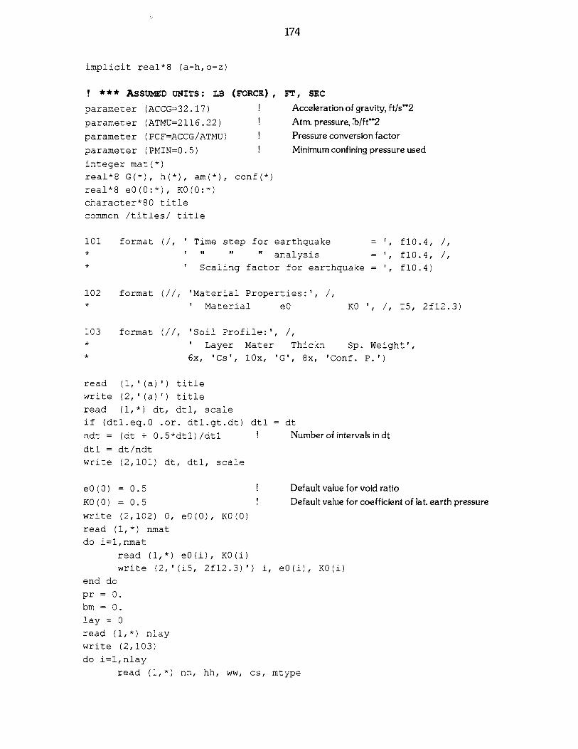
174
implicit real*8 (a-h,o-z)
! *** ASSUNED UNITS: LB
parameter (ACCG=32. 17)
parameter (ATMU=2116.22)
parameter (PCF=ACCG/ATMU)
parameter (PMIN=0 .5)
integer mat(*)
real*8 G(*), h(*), am(*),
real*8 e0(0:*), K0(0:*)
character*80 title
common /titles/ title
(FORCE),
conf(*)
FT, SEC
Acceleration of gravity, ft/s**2
Atm. pressure, lb/ft**2Pressure conversion factorMinimum confining pressure used
101 format (/, ' Time step for earthquake =* ' " " analysis =
* ' Scaling factor for earthquake =
102 format (//, 'Material Properties:', /,* ' Material eO KO ', /, I5, 2fl2.3)
103 format (//, 'Soil Profile:', /,
* ' Layer Mater Thickn Sp. Weight',
* 6x, 'Cs', lOx, 'G', 8x, 'Conf. P.')
read (1,'(a)') title
write (2,'(a)') title
read (1,*) dt, dtl, scale
if (dtl.eq.0 .or. dtl.gt.dt) dtl = dt
ndt = (dt + 0.5*dtl) /dtl Number of intervals in dt
dtl = dt/ndt
write (2,101) dt, dtl, scale
eO (0) = 0. 5 Default value for void ratio
KO (0) = 0. 5 Default value for coefficient of lat. earth pressure
write (2,102) 0, eO(O), KO(0)
read (1,*) nmat
do i=1,nmat
read (1,*) eO(i), KO(i)
write (2,'(i5, 2fl2.3)) i, eO(i), KO(i)
end do
pr = 0.
bm = 0.
lay = 0
read (1,*) nlay
write (2,103)
do i=1,nlay
read (1,*) nn, hh, ww, cs, mtype
f10.4, /,
f10.4, /,
fl0.4)
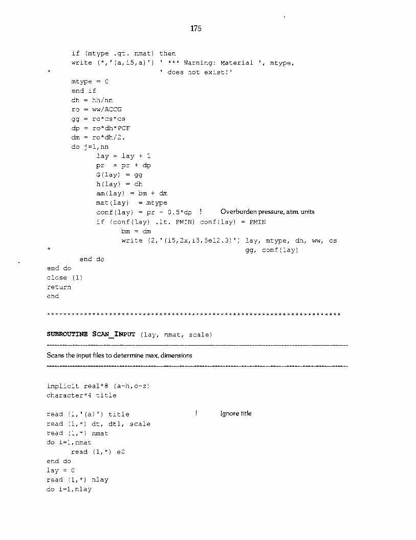
175
if (mtype .gt. nmat) then
write (*,'(a,i5,a)') '*** Warning: Material ', mtype,
* ' does not exist!'
mtype = 0
end if
dh = hh/nn
ro = ww/ACCG
gg = ro*cs*cs
dp = ro*dh*PCF
dm = ro*dh/2.
do j=1,nn
lay = lay + 1
pr = pr + dp
G(lay) = gg
h(lay) = dh
am(lay) = bm + dm
mat(lay) = mtype
conf (lay) = pr - 0. 5*dp ! Overburden pressure, atm. units
if (conf(lay) .lt. PMIN) conf(lay) = PMIN
bm = dm
write (2,'(i5,2x,i5,5e12.3)') lay, mtype, dh, ww, cs
* gg, conf(lay)
end do
end do
close (1)
return
end
SUBROUTINE SCANINPUT (lay, nimat, scale)
Scans the input files to determine max. dimensions
implicit real*8 (a-h,o-z)
character*4 title
read (1, ' (a) ') title Ignore title
read (1,*) dt, dtl, scale
read (1,*) nmat
do i=1,nmat
read (1,*) eO
end do
lay = 0
read (1,*) nlay
do i=1,nlay

176
read (1,*) nn
lay = lay + nn
end dorewind 1return
end
I;