Scale-dependent correlations between soil propertiesand environmental factors across the Loess Plateau of China

Zhi-Peng LiuA,C, Ming-An ShaoB,D, and Yun-Qiang WangB

AState Key Laboratory of Soil Erosion and Dry-land Farming on the Loess Plateau, Institute of Soil and WaterConservation, Chinese Academy of Sciences, Ministry of Water Resources, Yangling Shaanxi 712100,P.R. China.

BKey Laboratory of EcosystemObservation andModeling, Institute of Geographic Sciences and Natural ResourcesResearch, Chinese Academy of Sciences, Beijing 100101, P.R. China.

CGraduate School of Chinese Academy of Sciences, Beijing 100049, P.R. China.DCorresponding author. Email: shaoma@igsnrr.ac.cn

Abstract. Traditional statistical analysis of the correlations between spatially distributed variables takes no account oftheir regionalised nature. Factorial kriging analysis (FKA) was developed and widely used to overcome this problem. In ourstudy, we applied FKA to investigate scale-dependent correlations between selected soil properties and environmentalfactors across the Loess Plateau of China. Surface soil samples were collected from 382 sampling sites throughout theregion, and soil organic carbon (SOC), soil total nitrogen (STN), soil total phosphorus (STP), soil total potassium (STK),soil pH, bulk density (BD), and clay and silt contents were determined. Five environmental factors (elevation, precipitation,temperature, land-use type, and soil type) were also included in the FKA to identify influential processes. A linear model ofco-regionalisation, including a nugget effect and two spherical structures (effective ranges of 200 and 400 km), was fitted tothe experimental auto- and cross-variograms of the variables. Scale-dependent correlations were calculated for nugget-effect scale (<30–50 km), short-range scale with a range of 200 km, and long-range scale with a range of 400 km. Principalcomponent analysis was conducted to clearly illustrate the correlations at each spatial scale. The scale-dependentcorrelations were different from the general correlations and varied at different scales. Generally, SOC and STN werestrongly correlated at the nugget-effect scale and the long-range scale, but not at the short-range scale. Precipitation andclay content showed close correlations with STP at the nugget-effect scale and long-range scale. The STK was weaklycorrelated with the other variables at each spatial scale, and closely correlated with soil type at the long-range scale. Soil pHwas closely correlated with BD, soil type, and elevation at the nugget-effect, short, and long spatial scales, respectively.Close correlations were found between BD and land-use type at each spatial scale. Land use and soil type were consideredto be the important factors controlling spatial variation of soil properties at the short-range scale, while at the long-rangescale the likely factors were identified as precipitation, temperature, and elevation. Our study provided an insight into thespatial-dependent correlations between soil properties and environmental factors from a regional perspective.

Additional keywords: environmental factors, factorial kriging, Loess Plateau, soil properties, multivariate geostatistics.

Received 13 July 2012, accepted 12 March 2013, published online 22 April 2013

Introduction

Soil development is affected by natural and anthropogenicfactors such as parent material, climate, vegetation,topography, land use, and cultivation (Jenny 1941). None ofthese factors is uniform over space; rather, they exhibit spatialheterogeneity. As a result, soil properties vary from place toplace, in both vertical and horizontal directions (Nielsen andBouma 1985). Taking such variations into account is imperativein order to improve understanding of soil and its properties(Heuvelink and Webster 2001). To that end, soil scientists havebeen investigating and quantifying these spatial heterogeneities.Geostatistical methods, which are based on regionalised variabletheory (Matheron 1963), have been widely applied in soilscience to reveal spatial variability and distribution patterns

of various soil properties at scales ranging from local toglobal (Goovaerts 1999; Heuvelink and Webster 2001).

Soil physical, chemical, and biological properties are closelyrelated to each other as well as to environmental factors, whichare in turn influenced by human activities. Given the spatialvariation of all these properties, it is reasonable to argue that theinteractions and correlations are scale-dependent (Goovaerts1992). To clarify such complex systems, multivariatetechniques such as principal component analysis (PCA),factor analysis, and canonical correlation analysis have beenemployed to explore the underlying processes (Zhang et al.1999; Tan et al. 2004; Abdul-Wahab et al. 2005; Gray et al.2009). However, most studies have failed to take account of thespatial correlations that may exist between these variables at

Journal compilation � CSIRO 2013 www.publish.csiro.au/journals/sr

CSIRO PUBLISHING

Soil Research, 2013, 51, 112–123http://dx.doi.org/10.1071/SR12190

different scales. Factorial kriging analysis (FKA), a combinationof geostatistics and multivariate analysis, was developed toidentify the scale-dependent correlation (Goovaerts 1992).Applications of FKA have been reported in various fields,including remote sensing (van Meirvenne and Goovaerts2002; Rodgers and Oliver 2007), geochemical exploration(Imrie et al. 2008), heavy metal pollution (Webster et al.1994; Xu and Tao 2004), and ecology (Castrignanò et al. 2000).

The Loess Plateau is one of the main agricultural regions innorth-west China. Its ecosystem is fragile, and sensitive toclimate change and human disturbance (Liu 1999). Naturaldrought conditions limit plant growth, which leads to lessorganic matter input to the soil. Serious soil erosion andintensive cultivation hinder the formation of soil aggregatesand decrease soil fertility (Tang 1991). To protect the localenvironment and sustain soil productivity, the Chinesegovernment has launched a set of ecosystem restorationprojects on the Loess Plateau (Ostwald and Chen 2006). Inthe last decade, many studies have been done in this region toinvestigate the spatial variation of various soil properties andtheir relationships with environmental factors, to provide basicguidance for application of these restoration projects (Qiu et al.2001; Li and Huang 2008; Hu et al. 2009; Wang et al. 2009; Liu

et al. 2011; Gao and Shao 2012). Most of these studies usedunivariate analysis or traditional multivariate analysis withoutconsidering the regionalised nature of the studied variables. Fewpublished studies use multivariate geostatistical analysis toclarify their scale-dependent correlations, especially from theregional perspective.

The primary goal of this study is to apply FKA on soilphysico-chemical properties—soil organic carbon (SOC), soiltotal nitrogen (STN), soil total phosphorus (STP), soil totalpotassium (STK), soil pH, clay content, silt content, bulkdensity (BD)—and pertinent environmental factors (elevation,precipitation, temperature, land use, soil type) to explore theirscale-dependent correlations across the entire Loess Plateauregion.

Materials and methods

Study area

The Loess Plateau region (338430–418160N, 1008540–1148330E)is in the north-west of China, between the upper and middlereaches of the Yellow River (Fig. 1, inset). It encompasses a totalarea of ~620 000 km2, which is 6.5% of the territory of China.This inland region is dominated by a temperate, arid, and semi-

(a)

(b)

Fig. 1. Location of the Loess Plateau region in China (inset) and the sampling sites.

Correlations between soil properties and environmental factors Soil Research 113

arid continental monsoon climate, with mean annualprecipitation ranging from 150 to 800mm, and mean annualtemperature ranging from 3.6 to 14.38C. Both precipitation andtemperature decrease along the south-east to north-westtransect. Stormy rainfall is frequent from June to September,and contributes 55–78% of the annual total precipitation.Evaporation ranges from 1200 to 1400mm and annual solarradiation varies from 5.0� 109 to 6.7� 109 J m–2 (He et al.2003). Annual accumulated temperature above 08C is3200�39008C. Loess-paleosol deposits cover most of thearea and range from 30 to 80m in thickness. The loessiallandforms include yuans (large, flat surface with littleerosion), ridges, hills, and gullies at elevations ranging from100 to 3000m (Yang and Shao 2000). The soils are mainlyderived from loess, and are of diverse types. Most of the soils areclay-loam in texture, being sandier in the north-west and clayierin the south-east (Yang and Shao 2000). Natural vegetation hasbeen largely destroyed by deforestation and cultivation.Generally, current vegetation zones change with precipitationfrom south-east to north-west, in the order forest, forest-steppe,typical steppe, desert-steppe, and steppe-desert zones (Wanget al. 2011). Due to intensive rainfall in summer and poorvegetation coverage, the region has suffered serious soilerosion and land degradation (Tang 1991).

Field sampling and laboratory analysis

During April–November 2008, a total of 382 sampling siteswere investigated across the entire Loess Plateau region (Fig. 1).Sampling routes were selected across the region to use theexisting road transportation system, with a spacing betweentwo adjacent routes of ~40 km. Sampling sites were generallydesignated along the selected sampling routes. The base intervalbetween two adjacent sites was also designed to be 40 km., Agrid 40 km by 40 km was placed over a digital elevation mapoverlying the selected road system for further guidance. In thefield, the actual interval between sampling sites was 30–50 km,taking into account the logistical problem of accessing the sites.The actual sampling sites were randomly selected to representthe major landform, land-use, and vegetation types within therange of vision. Soil samples were randomly collected withoutany foreknowledge on the sampling sites. At the regional scale,significant local variation within 30–50 km could hardly beidentified and interpreted. In our study, this part of thevariation could be then included in the nugget effects.

At each site, one disturbed composite soil sample fromsurface soil (0–20 cm) was collected by mixing fivereplications taken with an auger within a circle 10m indiameter. All samples were sealed in plastic bags anddelivered to the laboratory within 10 days. Afterwards, soilsamples were air-dried and crushed to pass either a 0.25- or a 2-mmmesh, for laboratory analysis. Additionally, one undisturbedsoil core (100 cm3 in volume) at each site was taken to measuresoil BD. The accurate coordinates of the sampling site, thelatitude, longitude, and elevation, were recorded with a GPSreceiver (eTrex Venture, 5m precision in the horizontaldirection; Garmin Ltd, Kansas City, USA). Other siteproperties were recorded: land-use type (cropland, forestland,grassland); plant species and vegetation coverage by visualobservation; site slope and aspect measured with a geological

compass; information on cultivation practice by inquiry of localpeople.

For each soil sample, several soil physical and chemicalproperties were measured. Soil BD (g cm–3) was determined bymeasuring the volume of each original soil core, and the drymass after oven-drying at 1058C. Soil clay content (<0.002mm,%) and silt content (0.002–0.005mm, %) were measured bylaser diffraction using a Mastersizer 2000 (Malvern Instruments,Malvern, England). Soil chemical analyses were as follows:SOC (g kg–1) using the Walkley-Black method (Nelson andSommers 1982), with the most frequently used correction factor(1.32) applied to adjust SOC data to full organic C recovery(Meersmans et al. 2009); STN (g kg–1) using the Kjeldahldigestion procedure (Bremner and Tabatabai 1972); STP (gkg–1) and STK (g kg–1) by alkaline digestion (2 g NaOH and0.25 g of <0.25-mm sieved soil, 4008C for 15min and 7208C for15min) followed by molybdate colourimetric measurement(Murphy and Riley 1962) and the flame photometric method(Boon 1945), respectively. Soil pH value was measured at a soilto water mass ratio of 1 : 2.5 by using a pHmeter equipped with acalibrated combined glass electrode (McLean 1982).

Climate and soil type data

Climate data, i.e. annual mean precipitation and temperature,were derived from the meteorological records (1951–2001) from68 weather stations distributed throughout the region (Wanget al. 2011). Continuous data surfaces of precipitation andtemperature were created by kriging interpolation, using thestation datasets. Then, the climate data were extracted from thesurfaces for each sampling site, according to its spatialcoordinate. Similarly, soil type data were extracted from a1 : 500 000 digital soil map at the order level (CRSMERLP1992). Seven soil orders were recognised, i.e. Primosols,Anthrosols, Isohumosols, Luvisol, Cambisol, Halosols, andAridisols (Gong 2003).

Statistical analyses

Classical statisticsBasic statistical parameters such as maximum, minimum,

mean, skewness, and kurtosis were calculated to check thedistribution patterns of all of the numerical variables, i.e.SOC, STN, STP, STK, pH, clay content, silt content, BD,elevation, precipitation, temperature (Table 1). The resultsindicated no extremely skewed distributions (Liu et al. 2011).Before further statistical analysis, all original data for thenumerical variables were standardised to zero mean and unitvariance in order remove the differences in magnitude (Bocchiet al. 2000). A correlation matrix of these variables wascalculated using Pearson correlation coefficients. Forcategorical variables, i.e. land-use type and soil type, theircorrelations with other variables were calculated usingSpearman correlation coefficients (Caruso and Cliff 1997).

Principal component analysis (PCA) was then performed toextract the latent roots and vectors of the correlation matrix, andscores of independent principal components (PCs) werecomputed. The first two eigenvectors were converted to thecorrelations between the original variables and the PCs, andcould be plotted in the unit circle in the plane of the first two PCs

114 Soil Research Z.-P. Liu et al.

(Webster et al. 1994). The relationships among studied variablescan be clearly read from the unit circle. A small distance betweentwo variables denoted close relationship between them. Classicalstatistical analysis was performed with R 2.12.1 (RDCT 2011).

Factorial kriging analysisThe theory underlying FKA has been described in several

publications (Goovaerts 1992; Webster et al. 1994;Wackernagel 1998). Here, we provided the major steps inFKA as applied to our data. First, the experimental auto- andcross-variograms of all variables were calculated using thegeneral computing formula:

guvðhÞ ¼1

2nðhÞXnðhÞ

i¼ 1

½ZuðxiÞ � Zuðxi þ hÞ�½ZvðxiÞ � Zvðxi þ hÞ�

ð1Þwhere guv(h) estimates the semivariance of the two variablesZu(x) and Zv(x) at any pair of places x and x +h separated by a lagof h, which in this study was treated as a scalar rather than avector; n(h) is number of pairs; and Zu(xi), Zu(xi + h), Zv(xi),Zv(xi+ h) are the measured values at location xi and xi+h,respectively. By changing h, the experimental cross-variogram was obtained for u„ v. If u= v then the equationbecomes the common form of calculating the auto-variogram. Inour study, little evidence of anisotropy was detected, indicatedby anisotropy ratios <2.5 (Trangmar et al. 1986). Therefore,omnidirectional variograms were calculated for each studiedvariable as well as the leading PCs from PCA of the originaldata.

We included the categorical variables into the FKA bydescribing their spatial variation with a probability function(Xu and Tao 2004). The spatial variation of land-use typeand soil type was calculated as:

pðhÞ ¼ 1nðhÞ

XnðhÞ

i¼ 1

W½SðxiÞ 6¼ Sðxi þ hÞ� ð2Þ

where p(h) estimates the proportion of point pairs separated bydistance h that belong to two different categories; n(h) is thenumber of paired points; xi and xi+h are the locations of the

samples; and W[S(xi) „ S(xi + h)] is an indicator function definedas:

W½SðxiÞ 6¼ Sðxi þ hÞ� ¼ 1 if SðxiÞ 6¼ Sðxi þ hÞ0; otherwise

�ð3Þ

Before fitting a model of co-regionalisation, we checked theauto-variograms of the leading PCs, which were calculated fromthe generalcorrelation matrix. To represent their structures, adouble-spherical model with a nugget effect was fitted to thevariograms, since it fitted better in a least-squares sense than anyother models. The model could be expressed as:

gðhÞ ¼ c0 þ c13h2a1

� 12

h

a1

� �3" #

þ c23h2a2

� 12

h

a2

� �3" #

for 0 � h � a1

gðhÞ ¼ c0 þ c1 þ c23h2a2

� 12

h

a2

� �3" #

for a1 < h � a2

gðhÞ ¼ c0 þ c1 þ c2 for a2 < hgð0Þ ¼ 0 ð4Þwhere h is the lag distance; c0 is the nugget variance; c1 and c2are the sill values of the short and long-range variance; and a1and a2 are the distance parameters of the short- and long-rangestructures, respectively.

According to the linear model of co-regionalisation (LMC),we assumed that all the auto- and cross-variograms are modelledas linear combinations of the same set of three basic variogramfunctions gk(h), k= 1, 2, 3, where k= 1 refers to the variance ath= 0, i.e. the nugget variance; k= 2 and k= 3 refer to the short-and long-range variance components, respectively. So, for anycouple of variables u and v, the variogram guv(h) has thefollowing form:

guvðhÞ ¼X3k¼ 1

bkuvgkðhÞ ð5Þ

where bkuv is a coefficient to be determined from the data. If u = vthen bkuu and bkvv were the coefficients for the calculated auto-variograms. The basic variograms and any of their combinationsmust belong to the family of conditional negative semi-definite

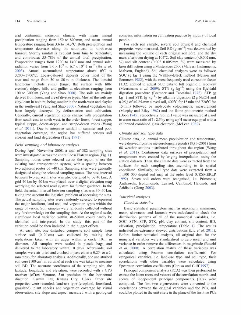
Table 1. Statistical summary of the selected soil properties and environmental factors across the Loess Plateau of ChinaSOC, Soil organic carbon; STN, soil total nitrogen; STP, soil total phosphorus; STK, soil total potassium; BD, soil bulk density; Elev., elevation; Prec.,

precipitation; Temp., temperature; s.d., standard deviation; CV, coefficient of variation

Variable Mean Max. Min. s.d. CV (%) Skewness Kurtosis

SOC (g kg–1) 10.04 54.03 0.43 7.02 70 2.58 10.07STN (g kg–1) 0.74 3.82 0.05 0.44 60 2.50 12.44STP (g kg–1) 0.63 2.79 0.17 0.24 38 2.79 18.88STK (g kg–1) 19.25 30.97 10.07 2.58 13 0.46 1.75pH 8.49 10.76 6.06 0.39 5 –1.07 10.51Clay (%) 19.78 35.80 0.40 7.93 40 –0.44 –0.68Silt (%) 68.94 84.70 6.30 12.83 19 –2.61 7.84BD (g cm–3) 1.34 1.82 1.02 0.15 11 0.49 –0.02Elev. (m) 1190 2978 99 517 43 –0.74 1.19Prec. (mm) 445 618 128 112 25 –0.08 –0.02Temp. (8C) 8.7 14.3 3.7 2.7 30 –0.66 –0.30

Correlations between soil properties and environmental factors Soil Research 115

functions (McBratney and Webster 1986). Therefore, thefollowing relations must hold for the coefficients bkuv:

bkuu � 0; bkvv � 0 and jbkuuj ¼ jbkvvj �ffiffiffiffiffiffiffiffiffiffiffiffibkuub

kvv

qð6Þ

Following the experience with modelling the variograms ofthe PCs, we fitted the whole set of auto- and cross-variogramswith two spherical functions plus nugget:

guvðhÞ ¼ b1uv þ b2uv3h2a1

� 12

h

a1

� �3" #

þ b3uv3h2a2

� 12

h

a2

� �3" #

ð7ÞFor parameters a1 and a2, we chose the same values

determined from the model of the PCs. Then the coefficientsb1uv, b

2uv, b

3uv were determined by fitting the model to variograms

using weighted least-squares algorithm under the constraint ofpositive semi-definiteness of the coefficients. We used the Rpackage ‘gstat’ (version 0.9–79) to perform the computing(Pebesma 2004).

The matrix of the coefficients bkuv was called a co-regionalisation matrix (Goovaerts 1992). It can provide thecorrelations of the studied variables at the spatial scale k,defined as:

rkuv ¼bkuvffiffiffiffiffiffiffiffiffiffiffiffibkuub

kvv

q ð8Þ

where rkuv is the structural correlation coefficient between Zu andZv at the spatial scale k. Based on the rk matrix, a PCA can beperformed to summarise relations between variables and help toidentify the underlying processes operating at the spatial scalesidentified.

Results

Classical statistical analysis

General correlations

General correlation coefficients were calculated from originaldata (Table 2). Most of the studied variables were, to some

extent, linearly correlated. We observed positive correlations ofSOC with STN and STP, but not with STK. Soil clay contentshowed positive correlations with SOC, STN, STP, STK, andtemperature. Positive correlation was detected betweentemperature and precipitation. Soil pH showed negativecorrelations with many variables, such as SOC, STN, STP,precipitation, temperature, and clay content. Elevation wasnegatively correlated with both temperature and precipitation.Negative correlation was also detected between silt content andBD. Many studies have reported similar results (Bai and Wang2011; Gao and Shao 2012). Here, soil type and land use showedfairly weak correlations with most of the variables. However, thegeneral correlation coefficients could not give any informationon spatial-dependent correlations between variables. Fairlyweak or strong correlations between variables could beattributed to the counteractions or overlays of differentcorrelation behaviours at various spatial scales (Xu and Tao2004). From this point of view, an application of FKA on ourdatasets could be more revealing in providing insights into theirscale-dependent interactions (Goovaerts and Webster 1994).

Principal component analysis

Principal component analysis is commonly used to reducedata dimensions and extract main variations by decomposing theoriginal data into several PCs. Each PC explains a percentage ofthe total variance, while the first few components generallyaccount for most of the variance. First, PCA was performed onthe correlation matrix of the original data. The cumulativepercentages of the variances explained by the first four PCs(eigenvalue >1) are listed in Table 3. The first two PCs couldexplain 30.9% and 14.3% of the total variance, respectively, andthe first four PCs accounted for 67% of the total variance.Correlation coefficients between the first two PCs and studiedvariables are also shown in Table 3. Negative correlations werefound between PC1 and SOC, STN, STP, STK, clay content, siltcontent, precipitation, temperature, and soil type; and betweenPC2 and SOC, STN, STK, pH, clay content, BD, elevation, andsoil type. Positive correlations were detected between PC1 andpH, BD, elevation, and land use; and between PC2 and siltcontent, precipitation, temperature, and land use. The

Table 2. Correlation coefficients between selected soil properties and environmental factors across the Loess Plateau of ChinaSOC, Soil organic carbon; STN, soil total nitrogen; STP, soil total phosphorus; STK, soil total potassium; BD, soil bulk density; Elev., elevation; Prec.,precipitation; Temp., temperature; LU, land-use type; ST, soil type. Coefficients for the categorical variables (LU, ST) with others are Spearman correlation

coefficients; all the other correlation coefficients are Pearson correlation coefficients

SOC STN STP STK pH Clay Silt BD Elev. Prec. Temp. LU

STN 0.923 1STP 0.411 0.461 1STK 0.103 0.153 0.213 1pH –0.456 –0.512 –0.375 –0.045 1Clay 0.307 0.422 0.465 0.313 –0.376 1Silt 0.143 0.204 0.263 –0.185 –0.227 0.291 1BD –0.272 –0.298 0.247 0.258 0.328 –0.204 –0.540 1Elev. –0.001 0.066 –0.168 0.023 0.283 –0.167 0.017 –0.003 1Prec. 0.221 0.248 0.286 –0.096 –0.501 0.318 0.286 –0.352 –0.475 1Temp. 0.122 0.182 0.223 0.151 –0.405 0.458 0.074 –0.141 –0.603 0.498 1LU –0.217 –0.204 –0.391 –0.198 0.296 –0.322 –0.137 0.092 0.172 –0.176 –0.141 1ST 0.135 0.139 0.046 0.133 0.012 0.091 –0.191 0.153 –0.020 –0.217 0.013 –0.053

116 Soil Research Z.-P. Liu et al.

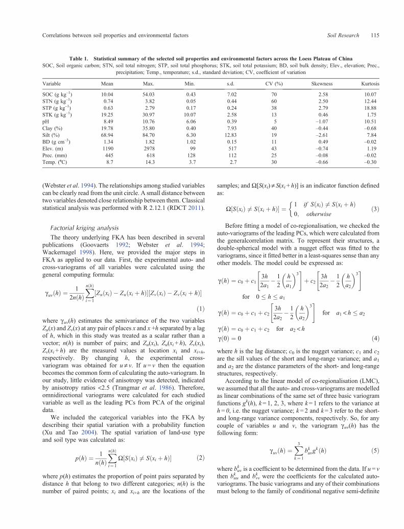
correlations were projected into a unit circle in the plane of thefirst two PCs in Fig. 2a. In the lower left quadrant, SOC wasclosely related to STN, and STP was strongly associated withclay content. Soil silt content was close to temperature andprecipitation in the upper left quadrant. Soil type showed a closerelationship with STK. Soil BD was relatively close to elevationin the lower right quadrant. Soil pH and land use were distinctfrom the other variables.

Spatial analysis and co-regionalisation

Linear model of co-regionalisation

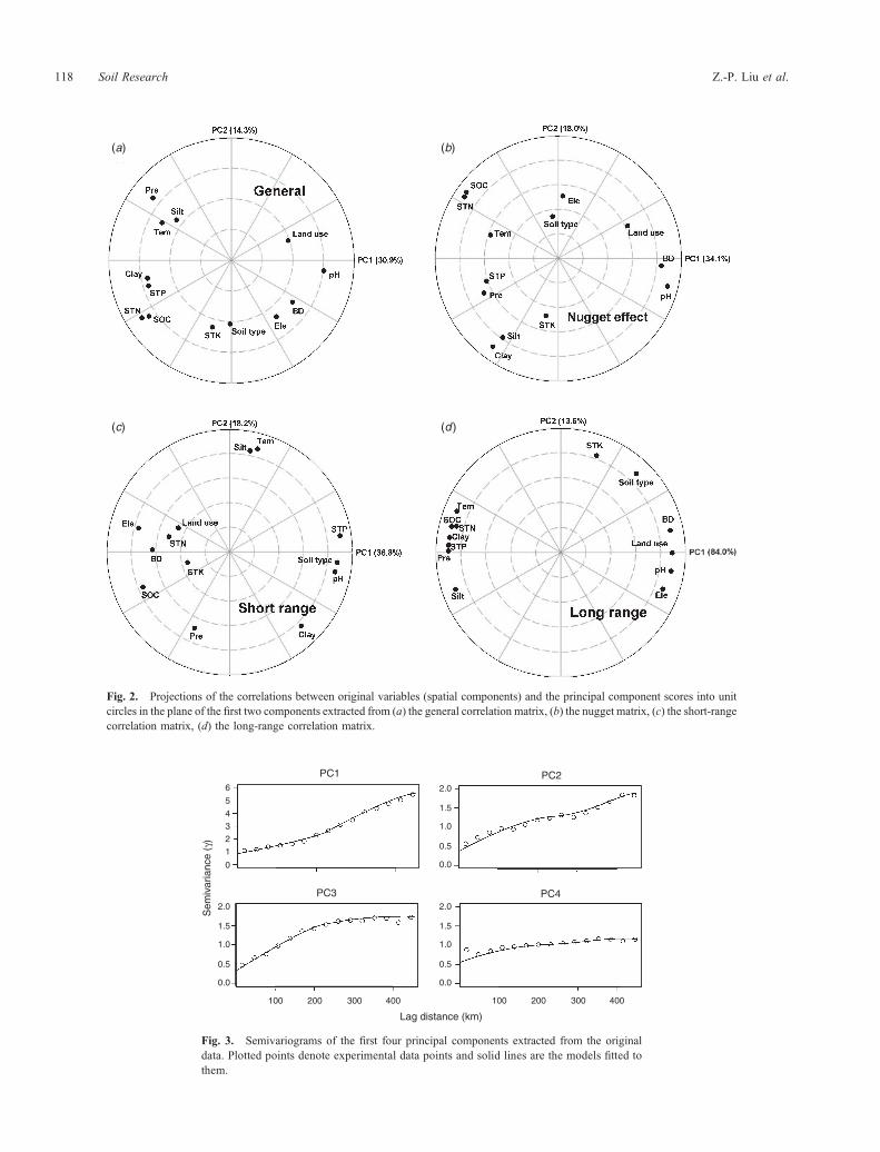
Based on the eigenvectors extracted by PCA, the scores of thePCs were calculated as a linear combination of the standardiseddata of all the variables. Auto-variograms were first calculatedfor the leading PCs scores to check the systematic spatialpatterns. As shown in Fig. 3, the first PC showed a long-range spatial dependence with a maximum spatial range of400 km, while the short-range spatial range was ~200 km.Similar spatial structures were detected on PC2. A short-range structure was obvious with PC3, which had spatialdependence within the lag distance <200 km. Explaining 8%of the total variance, PC4 showed a weak spatial structure withina spatial range of ~400 km. According to Goovaerts (1992),three basic variogram functions gk(h) are sufficient to avoid theinstability of the estimation: nugget effect and two otherauthorised functions. Thus, we chose the values of 200 kmand 400 km as the distance parameters (a1 and a2 in Eqn 7)for short-range and long-range structures to fit a linear model ofco-regionalisation.

Some of the 91 experimental auto- and cross-variograms withtheir fitted models are shown in Fig. 4. Generally, four distinctpatterns can be observed from the plotted points and fitted lines.For SOC, STP, and land use, semivariances (or probability)increased gradually in a low slope with increasing lag distance,

and then reached the maximum value at a long range of ~400 km.Nugget variance shows a considerable contribution to the totalvariation in these variograms. In our study, the variations withinshortest sampling intervals (30–50 km) and experimental errorwere sorted to the nugget effect. A similar long-range structure,but with a relatively sharp increasing slope, was displayed bysoil pH, silt content, BD, SOC–STN, SOC–STP, SOC–claycontent, STP–clay content, and STK–clay content. A short-range structure, represented by STK, soil type, and STK–BD,displayed a steady increase of semivariance (or probability) in asharp slope until a maximum spatial range of ~200 km. Adecreasing trend of semivariance was represented by some ofthe cross-variograms, such as pH–silt content and claycontent–BD. These different spatial structures reflect variousspatial variations of the corresponding variables or pair ofvariables at different spatial scales. Therefore, therelationships between these regionalised variables should beconsidered as scale-dependent interactions. To clarify thesescale-dependent correlations, the parameters, bk, from thefitted model of co-regionalisation were used to calculate thecorrelation coefficients between the studied variables at the scalek (Eqn 8).

Scale-dependent correlation coefficients

In our study, the spatial variation of each variable wasdecomposed into three components, i.e. nugget effect, short-range component with a range of 200 km, and long-rangecomponent with a range of 400 km. According to these threecomponents, the scale-dependent correlations between thestudied variables can be represented at each specific scale(Table 4), by filtering the variation from the other scales.

At the nugget-effect scale, i.e. the range less than the smallestsampling interval, high positive correlations were foundbetween SOC and STN, between clay and silt content, andbetween precipitation and temperature, while negativecorrelations were between pH and STN, and betweenelevation and precipitation. These correlations were, to someextent, similar to the general correlations discussed above.However, some of the relatively strong correlations in generalcorrelations were not detected at this scale, such as thecorrelations between STN and STP, between pH and STN,and between silt and BD.

After filtering out the nugget effect, elevation showed highnegative correlations with clay content and STP at the short-range scale. This could be explained by the transportation oferoded fine soil particles, together with attached or dissolved soilP from higher to lower elevations (Shi and Shao 2000). Therewere some other differences between short-range structurecorrelations and nugget-effect correlations. For example, thecorrelations between silt and clay content changed from highlypositive in nugget variances to highly negative in short-rangestructures. In contrast, the correlation between soil pH and STPchanged from negative in nugget variances to highly positive inshort-range structure. Also, the strong positive correlationbetween SOC and STN became relatively weak at the short-range scale. Notably, the effects of soil type on STN, STP,soil pH, and land use seemed to be apparent at the short-rangescale.

Table 3. Correlations between selected variables with principalcomponents (PCs) from the original data

SOC, Soil organic carbon; STN, soil total nitrogen; STP, soil totalphosphorus; STK, soil total potassium; BD, soil bulk density; Elev.,elevation; Prec., precipitation; Temp., temperature; LU, land-use type;

ST, soil type

Variables PC1 PC2 PC3 PC4

SOC –0.673 –0.453 –0.288 0.375STN –0.729 –0.464 –0.292 0.301STP –0.675 –0.205 0.007 –0.285STK –0.156 –0.541 0.454 –0.367pH 0.753 –0.082 –0.001 –0.180Clay –0.683 –0.143 0.192 –0.308Silt –0.446 0.333 –0.504 –0.354BD 0.496 –0.337 0.550 0.044Elev. 0.366 –0.455 –0.624 –0.216Prec. –0.640 0.509 0.117 0.129Temp. –0.569 0.309 0.549 0.143LU 0.462 0.164 –0.173 0.464ST –0.011 –0.514 0.239 0.305

Eigenvalue 4.02 1.86 1.76 1.09% of Variance 30.9 14.3 13.8 8.0Cumulative variance % 30.9 45.2 59.0 67.0

Correlations between soil properties and environmental factors Soil Research 117

(a) (b)

(c) (d )

Fig. 2. Projections of the correlations between original variables (spatial components) and the principal component scores into unitcircles in the plane of the first two components extracted from (a) the general correlation matrix, (b) the nugget matrix, (c) the short-rangecorrelation matrix, (d) the long-range correlation matrix.

6

PC1 PC2

PC4PC3

5

4321

0

2.0

1.5

1.0

0.5

0.0

2.0

1.5

1.0

0.5

0.0

2.0

1.5

1.0

0.5

0.0

100 200 300 400

Lag distance (km)

Sem

ivar

ianc

e (γ

)

100 200 300 400

Fig. 3. Semivariograms of the first four principal components extracted from the originaldata. Plotted points denote experimental data points and solid lines are the models fitted tothem.

118 Soil Research Z.-P. Liu et al.

1.0

SOC

STK

Silt

Land use

SOC-STN

SOC-Clay

STK-Clay

pH-Silt Clay-BD

STK-BD

STP-Clay

SOC-STP

Soil type

BD

pH

STP

1.0

0.6

0.2

1.4

1.0

0.6

0.2

1.4

1.0

0.6

0.2

5.0

4.0

3.0

2.0

0.4

0.2

0.0

0.6

0.4

0.2

0.0

0.3

0.1

0.1

–0.1

–0.1

–0.3

–0.5

0.6

0.2

1.0

1.4

1.0

0.6

0.2

0.8

0.7

0.6

0.5

0.9

0.7

0.5

0.4

0.2

0.0

0.4

0.3

0.2

0.1

0.0

–0.1

–0.3

–0.5

100 200 300 400 100 200

Lag distance (km)

Sem

ivar

ianc

e (γ

)

Sem

ivar

ianc

e (γ

)S

emiv

aria

nce

(γ)

Sem

ivar

ianc

e (γ

)S

emiv

aria

nce

(γ)

Sem

ivar

ianc

e (γ

)S

emiv

aria

nce

(γ)

Sem

ivar

ianc

e (γ

)

Sem

ivar

ianc

e (γ

)S

emiv

aria

nce

(γ)

Sem

ivar

ianc

e (γ

)S

emiv

aria

nce

(γ)

Sem

ivar

ianc

e (γ

)S

emiv

aria

nce

(γ)

Pro

babi

lity

Pro

babi

lity

300 400

0.4

0.6

0.2

Fig. 4. Some of the 91 auto- and cross-variograms of the selected soil properties andenvironmental factors. Plotted points denote experimental data points and solid lines aremodels fitted to them.

Correlations between soil properties and environmental factors Soil Research 119

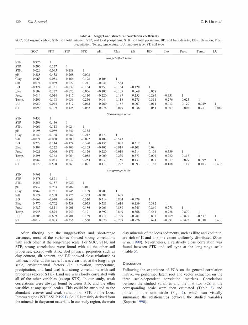
After filtering out the nugget-effect and short-rangevariances, most of the variables showed strong correlationswith each other at the long-range scale. For SOC, STN, andSTP, strong correlations were found with all the other soilproperties, except with STK. Soil physical properties such asclay content, silt content, and BD showed close relationshipswith each other at this scale. It was clear that, at the long-rangescale, environmental factors (i.e. elevation, temperature,precipitation, and land use) had strong correlations with soilproperties (except STK). Land use was closely correlated withall of the other variables (except STK). In our study, weakcorrelations were always found between STK and the othervariables at any spatial scales. This could be attributed to theabundant reserves and weak variation of STK on the LoessPlateau region (ISTCASLP 1991). Soil K is mainly derived fromthe minerals in the parent materials. In our study region, the main

clay minerals of the loess sediments, such as illite and kaolinite,are rich of K and to some extent uniformly distributed (Zhaoet al. 1999). Nevertheless, a relatively close correlation wasfound between STK and soil type at the long-range scale(Table 5).

Discussion

Following the experience of PCA on the general correlationmatrix, we performed latent root and vector extraction on thethree scale-dependent correlation matrices. Correlationsbetween the studied variables and the first two PCs at thecorresponding scale were then estimated (Table 5) andplotted in the unit circle (Fig. 2), which can visuallysummarise the relationships between the studied variables(Saporta 1990).

Table 4. Nugget and structural correlation coefficientsSOC, Soil organic carbon; STN, soil total nitrogen; STP, soil total phosphorus; STK, soil total potassium; BD, soil bulk density; Elev., elevation; Prec.,

precipitation; Temp., temperature; LU, land-use type; ST, soil type

SOC STN STP STK pH Clay Silt BD Elev. Prec. Temp. LU

Nugget-effect scaleSTN 0.976 1STP 0.206 0.227 1STK 0.026 0.045 0.188 1pH –0.388 –0.452 –0.268 –0.003 1Clay 0.063 0.053 0.166 0.198 –0.104 1Silt 0.074 0.069 0.027 0.241 –0.041 0.584 1BD –0.324 –0.331 –0.037 –0.134 0.353 –0.154 –0.128 1Elev. 0.109 0.137 –0.075 0.056 –0.107 –0.139 0.069 0.058 1Prec. 0.014 0.014 0.117 –0.110 –0.220 0.197 0.255 –0.294 –0.331 1Temp. 0.206 0.198 0.039 –0.256 –0.044 0.118 0.275 –0.311 0.276 0.625 1LU –0.050 –0.044 –0.312 –0.042 0.269 –0.187 0.007 –0.011 –0.013 –0.129 0.029 1ST 0.090 0.109 –0.125 –0.062 –0.076 0.049 0.038 0.051 –0.007 0.002 0.251 0.062

Short-range scaleSTN 0.433 1STP –0.209 –0.436 1STK –0.066 0.118 –0.024 1pH –0.198 –0.089 0.649 –0.335 1Clay –0.149 –0.188 0.082 –0.217 0.277 1Silt –0.071 –0.060 0.303 –0.092 0.102 –0.543 1BD 0.228 0.314 –0.124 0.390 –0.135 0.081 0.312 1Elev. 0.304 0.222 –0.700 –0.163 –0.405 –0.919 –0.201 0.09 1Prec. 0.021 0.096 –0.175 –0.126 0.220 –0.016 –0.214 0.176 0.339 1Temp. –0.395 –0.362 0.064 –0.055 –0.009 –0.239 0.373 –0.004 0.282 –0.316 1LU 0.082 0.033 0.032 –0.254 –0.033 –0.150 0.133 0.077 –0.017 0.029 –0.099 1ST –0.179 –0.500 0.56 –0.091 0.417 0.222 0.093 –0.188 –0.188 0.117 0.103 –0.636

Long-range scaleSTN 0.961 1STP 0.878 0.871 1STK 0.253 0.187 –0.020 1pH –0.937 –0.964 –0.907 0.041 1Clay 0.967 0.931 0.945 0.189 –0.907 1Silt 0.524 0.508 0.775 –0.363 –0.581 0.699 1BD –0.669 –0.640 –0.849 0.310 0.714 0.804 –0.979 1Elev. 0.770 –0.702 –0.538 0.053 0.781 –0.616 –0.139 0.382 1Prec. 0.887 0.811 0.901 –0.186 –0.905 0.889 0.745 –0.860 –0.778 1Temp. 0.948 0.874 0.750 0.171 –0.892 0.849 0.368 –0.564 –0.928 0.870 1LU –0.708 –0.609 –0.901 0.139 0.711 –0.799 –0.781 0.833 0.469 –0.877 –0.637 1ST –0.019 0.083 –0.356 0.560 0.070 –0.209 –0.776 0.694 –0.091 –0.422 0.038 0.630

120 Soil Research Z.-P. Liu et al.

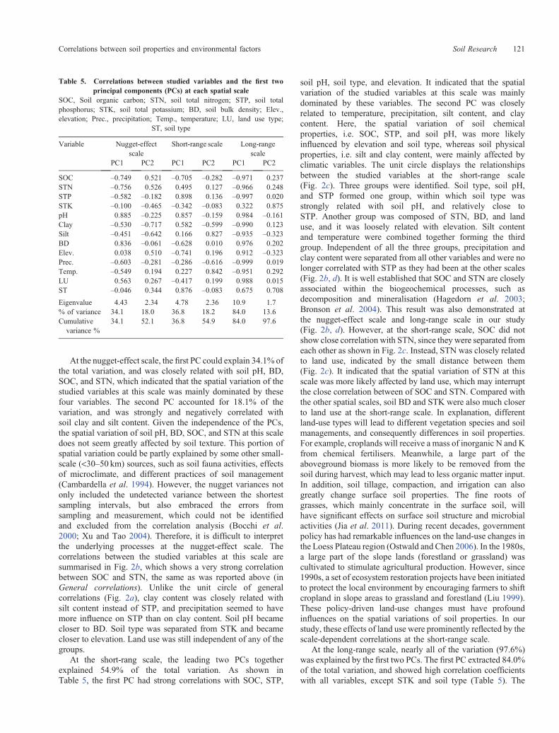
At the nugget-effect scale, the first PC could explain 34.1% ofthe total variation, and was closely related with soil pH, BD,SOC, and STN, which indicated that the spatial variation of thestudied variables at this scale was mainly dominated by thesefour variables. The second PC accounted for 18.1% of thevariation, and was strongly and negatively correlated withsoil clay and silt content. Given the independence of the PCs,the spatial variation of soil pH, BD, SOC, and STN at this scaledoes not seem greatly affected by soil texture. This portion ofspatial variation could be partly explained by some other small-scale (<30–50 km) sources, such as soil fauna activities, effectsof microclimate, and different practices of soil management(Cambardella et al. 1994). However, the nugget variances notonly included the undetected variance between the shortestsampling intervals, but also embraced the errors fromsampling and measurement, which could not be identifiedand excluded from the correlation analysis (Bocchi et al.2000; Xu and Tao 2004). Therefore, it is difficult to interpretthe underlying processes at the nugget-effect scale. Thecorrelations between the studied variables at this scale aresummarised in Fig. 2b, which shows a very strong correlationbetween SOC and STN, the same as was reported above (inGeneral correlations). Unlike the unit circle of generalcorrelations (Fig. 2a), clay content was closely related withsilt content instead of STP, and precipitation seemed to havemore influence on STP than on clay content. Soil pH becamecloser to BD. Soil type was separated from STK and becamecloser to elevation. Land use was still independent of any of thegroups.

At the short-rang scale, the leading two PCs togetherexplained 54.9% of the total variation. As shown inTable 5, the first PC had strong correlations with SOC, STP,

soil pH, soil type, and elevation. It indicated that the spatialvariation of the studied variables at this scale was mainlydominated by these variables. The second PC was closelyrelated to temperature, precipitation, silt content, and claycontent. Here, the spatial variation of soil chemicalproperties, i.e. SOC, STP, and soil pH, was more likelyinfluenced by elevation and soil type, whereas soil physicalproperties, i.e. silt and clay content, were mainly affected byclimatic variables. The unit circle displays the relationshipsbetween the studied variables at the short-range scale(Fig. 2c). Three groups were identified. Soil type, soil pH,and STP formed one group, within which soil type wasstrongly related with soil pH, and relatively close toSTP. Another group was composed of STN, BD, and landuse, and it was loosely related with elevation. Silt contentand temperature were combined together forming the thirdgroup. Independent of all the three groups, precipitation andclay content were separated from all other variables and were nolonger correlated with STP as they had been at the other scales(Fig. 2b, d). It is well established that SOC and STN are closelyassociated within the biogeochemical processes, such asdecomposition and mineralisation (Hagedorn et al. 2003;Bronson et al. 2004). This result was also demonstrated atthe nugget-effect scale and long-range scale in our study(Fig. 2b, d). However, at the short-range scale, SOC did notshow close correlation with STN, since they were separated fromeach other as shown in Fig. 2c. Instead, STN was closely relatedto land use, indicated by the small distance between them(Fig. 2c). It indicated that the spatial variation of STN at thisscale was more likely affected by land use, which may interruptthe close correlation between of SOC and STN. Compared withthe other spatial scales, soil BD and STK were also much closerto land use at the short-range scale. In explanation, differentland-use types will lead to different vegetation species and soilmanagements, and consequently differences in soil properties.For example, croplands will receive a mass of inorganic N and Kfrom chemical fertilisers. Meanwhile, a large part of theaboveground biomass is more likely to be removed from thesoil during harvest, which may lead to less organic matter input.In addition, soil tillage, compaction, and irrigation can alsogreatly change surface soil properties. The fine roots ofgrasses, which mainly concentrate in the surface soil, willhave significant effects on surface soil structure and microbialactivities (Jia et al. 2011). During recent decades, governmentpolicy has had remarkable influences on the land-use changes inthe Loess Plateau region (Ostwald and Chen 2006). In the 1980s,a large part of the slope lands (forestland or grassland) wascultivated to stimulate agricultural production. However, since1990s, a set of ecosystem restoration projects have been initiatedto protect the local environment by encouraging farmers to shiftcropland in slope areas to grassland and forestland (Liu 1999).These policy-driven land-use changes must have profoundinfluences on the spatial variations of soil properties. In ourstudy, these effects of land use were prominently reflected by thescale-dependent correlations at the short-range scale.

At the long-range scale, nearly all of the variation (97.6%)was explained by the first two PCs. The first PC extracted 84.0%of the total variation, and showed high correlation coefficientswith all variables, except STK and soil type (Table 5). The

Table 5. Correlations between studied variables and the first twoprincipal components (PCs) at each spatial scale

SOC, Soil organic carbon; STN, soil total nitrogen; STP, soil totalphosphorus; STK, soil total potassium; BD, soil bulk density; Elev.,elevation; Prec., precipitation; Temp., temperature; LU, land use type;

ST, soil type

Variable Nugget-effectscale

Short-range scale Long-rangescale

PC1 PC2 PC1 PC2 PC1 PC2

SOC –0.749 0.521 –0.705 –0.282 –0.971 0.237STN –0.756 0.526 0.495 0.127 –0.966 0.248STP –0.582 –0.182 0.898 0.136 –0.997 0.020STK –0.100 –0.465 –0.342 –0.083 0.322 0.875pH 0.885 –0.225 0.857 –0.159 0.984 –0.161Clay –0.530 –0.717 0.582 –0.599 –0.990 0.123Silt –0.451 –0.642 0.166 0.827 –0.935 –0.323BD 0.836 –0.061 –0.628 0.010 0.976 0.202Elev. 0.038 0.510 –0.741 0.196 0.912 –0.323Prec. –0.603 –0.281 –0.286 –0.616 –0.999 0.019Temp. –0.549 0.194 0.227 0.842 –0.951 0.292LU 0.563 0.267 –0.417 0.199 0.988 0.015ST –0.046 0.344 0.876 –0.083 0.675 0.708

Eigenvalue 4.43 2.34 4.78 2.36 10.9 1.7% of variance 34.1 18.0 36.8 18.2 84.0 13.6Cumulative

variance %34.1 52.1 36.8 54.9 84.0 97.6

Correlations between soil properties and environmental factors Soil Research 121

second PC accounted for the remaining 13.6% of the variance,and was positively correlated with STK and soil type. As shownin Fig. 2d, the studied variables were clustered into two groups.One group comprised SOC, STN, STP, temperature,precipitation, and clay content. Within the group, SOC andSTN were closely combined together and located betweenclay content and temperature. Clay content and STP werehighly correlated with precipitation. This indicated thatprecipitation and temperature could be the main factorsimpacting these soil chemical and physical properties at thisspatial scale. It has been reported that climatic variables couldcontrol large-scale soil variation by determining regional waterand heat distribution (Jenny 1941;Wang et al. 2011). Vegetationzones, which change according to the climate zones, can directlydetermine the quantity and quality of organic matter input to thesoil, and consequently the spatial variation of SOC andSTN. Weathering processes, which were physically controlledby climate, would greatly influence the formation of clayminerals and the release of P from the parent material (Linet al. 2009). The other group comprised soil pH, BD, land use,and elevation. Here, soil pH was more likely to be affected byelevation instead of soil type as at the short-range scale. At thisscale, elevation might also be considered as a large-scaleimpacting factor, since it showed much closer correlationswith precipitation and temperature than at the other spatialscales (Table 4). Soil type and STK were relatively close toeach other, while clearly separated from both of the clusteredgroups. At the long-range scale, the appearances of strongcorrelations between most of the variables should beattributed to the effect of filtering out the local and short-range variation, as well as the experimental error.

Conclusion

Factorial kriging analysis was applied to explore the scale-dependent correlations between selected variables across theLoess Plateau region, including eight surface soil properties (i.e.SOC, STN, STP, STK, soil pH, clay content, silt content, andBD), and five pertinent environmental factors (i.e. elevation,precipitation, temperature, land use, and soil type). The linearmodel of co-regionalisation was fitted by a nugget plus double-spherical model with a short-range scale of 200 km and a long-range scale of 400 km. Scale-dependent correlations were muchdifferent from the general correlations and varied at differentspatial scales. Generally, for nugget variances, close correlationswere found between SOC and STN, precipitation and STP, siltand clay content, and soil pH and BD. Soil type and land use didnot show a significant effect at this scale. At the short-rangescale, BD and STN were more correlated with land use. Soil pHwas closely correlated with soil type, and temperature showedstrong correlation with silt content. However, the correlationbetween SOC and STN was found to be relatively weak at thisscale, which could probably be explained by the effect of landuse. Clay content and precipitation did not show closecorrelations with the other variables. At the long-range scale,high correlation coefficients were found between most of thevariables. Precipitation and temperature seemed to have greatinfluence on SOC, STN, STP, and clay content. Soil pH wasmore likely to be affected by elevation. Our results showed that

STK was weakly correlated with the other variables at eachspatial scale, except with soil type at the long-range scale.

From a regional perspective, our study provided aquantitative insight into the complex interactions betweenstudied soil properties and environmental factors at differentspatial scales. More investigation is needed for the furtherunderstanding of the underlying processes controlling thesescale-dependent correlations.

Acknowledgments

This research was supported by the Innovation Team Program of the ChineseAcademy of Sciences, the Program for Innovative Research Team ofMinistry of Education, China (No. IRT0749), and the National NaturalScience Foundation of China (No. 41071156 and No.51179180). Authorsthank the editor and reviewers for their valuable comments and suggestions.

References

Abdul-Wahab SA, Bakheit CS, Al-Alawi SM (2005) Principal componentand multiple regression analysis in modelling of ground-level ozone andfactors affecting its concentrations. Environmental Modelling &Software 20, 1263–1271. doi:10.1016/j.envsoft.2004.09.001

Bai Y, Wang Y (2011) Spatial variability of soil chemical properties in aJujube slope on the Loess Plateau of China. Soil Science 176, 550–558.doi:10.1097/SS.0b013e3182285cfd

Bocchi S, Castrignan A, Fornarò F, Maggiore T (2000) Application offactorial kriging for mapping soil variation at field scale. EuropeanJournal of Agronomy 13, 295–308. doi:10.1016/S1161-0301(00)00061-7

Boon SD (1945) ‘Vlam-Fotmetrie.’ (Centen: Amsterdam)Bronson KF, Zobeck TM, Chua TT, Acosta-Martinez V, van Pelt RS,

Booker JD (2004) Carbon and nitrogen pools of southern high plainsand grassland soils. Soil Science Society of America Journal 68,1695–1704. doi:10.2136/sssaj2004.1695

Bremner JM, Tabatabai MA (1972) Use of an ammonia electrode fordetermination of ammonia in Kjeldahl. Communications in SoilScience and Plant Analysis 3, 159–165. doi:10.1080/00103627209366361

Cambardella CA, Moorman TB, Novak JM, Parkin TB, Karlen DL, TurcoRF, Konopka AE (1994) Field-scale variability of soil properties inCentral Iowa soils. Soil Science Society of America Journal 58,1501–1511. doi:10.2136/sssaj1994.03615995005800050033x

Caruso JC, Cliff N (1997) Empirical size, coverage, and power of confidenceintervals for Spearman’s Rho. Educational and PsychologicalMeasurement 57, 637–654. doi:10.1177/0013164497057004009

Castrignanò A, Goovaerts P, Lulli L, Bragato G (2000) A geostatisticalapproach to estimate probability of occurrence of Tuber melanosporumin relation to some soil properties. Geoderma 98, 95–113. doi:10.1016/S0016-7061(00)00054-9

Committee of Remote Sensing Maps of the Environment and Resources onthe Loess Plateau (1992) 1 : 500000 digital soil map of the Loess Plateauregion. (Seismological Press: Beijing)

Gao L, Shao MA (2012) The interpolation accuracy for seven soil propertiesat various sampling scales on the Loess Plateau, China. Journal of Soilsand Sediments 12, 128–142. doi:10.1007/s11368-011-0438-0

Gong ZT (2003) ‘Chinese Soil Taxonomy: theory, method, practice.’(Science Press: Beijing)

Goovaerts P (1992) Factorial kriging analysis: a useful tool for exploring thestructure of multivariate spatial soil information. Journal of Soil Science43, 597–619. doi:10.1111/j.1365-2389.1992.tb00163.x

Goovaerts P (1999) Geostatistics in soil science: state-of-the-art andperspectives.Geoderma 89, 1–45. doi:10.1016/S0016-7061(98)00078-0

122 Soil Research Z.-P. Liu et al.

Goovaerts P, Webster R (1994) Scale-dependent correlation between topsoilcopper and cobalt concentrations in Scotland. European Journal of SoilScience 45, 79–95. doi:10.1111/j.1365-2389.1994.tb00489.x

Gray JM, Humphreys GS, Deckers JA (2009) Relationships in soildistribution as revealed by a global soil database. Geoderma 150,309–323. doi:10.1016/j.geoderma.2009.02.012

Hagedorn F, Spinnler D, Siegwolf R (2003) Increase N deposition retardsmineralization of old soil organic matter. Soil Biology & Biochemistry35, 1683–1692. doi:10.1016/j.soilbio.2003.08.015

He XB, Li ZB, Hao MD, Tang KL, Zheng FL (2003) Down-scale analysisfor water scarcity in response to soil-water conservation on LoessPlateau of China. Agriculture, Ecosystems & Environment 94,355–361. doi:10.1016/S0167-8809(02)00039-7

Heuvelink GBM, Webster R (2001) Modelling soil variation: past, presentand future. Geoderma 100, 269–301. doi:10.1016/S0016-7061(01)00025-8

Hu W, Shao MA, Wang QJ, Fan J, Horton R (2009) Temporal changes ofsoil hydraulic properties under different land uses. Geoderma 149,355–366. doi:10.1016/j.geoderma.2008.12.016

Imrie CE, Korre A, Munoz-Melendez G, Thornton I, Durucan S (2008)Application of factorial kriging analysis to the FOREGS Europeantopsoil geochemistry database. The Science of the Total Environment393, 96–110. doi:10.1016/j.scitotenv.2007.12.012

Integrated Survey Team of Chinese Academy of Sciences on the LoessPlateau (1991) ‘Soil resources and its rational use on the Loess Plateau.’pp. 171–173. (Chinese Science and Technology Press: Beijing)

Jenny (1941) ‘Factors of soil formation: a system of quantitative pedology.’(McGraw-Hill: New York) (Reprinted by Dover Publications: NewYork)

Jia XX, Shao MA, Wei XR, Horton R, Li XZ (2011) Estimating total netprimary productivity of managed grasslands by a state-space modelingapproach in a small catchment on the Loess Plateau, China. Geoderma160, 281–291. doi:10.1016/j.geoderma.2010.09.016

Li YS, Huang MB (2008) Pasture yield and soil water depletion ofcontinuous growing alfalfa in the Loess Plateau of China.Agriculture, Ecosystems & Environment 124, 24–32. doi:10.1016/j.agee.2007.08.007

Lin JS, Shi XZ, Lu XX, Yu DS,WangHJ, Zhao YC, SunWX (2009) Storageand spatial variation of phosphorus in paddy soils of China. Pedosphere19, 790–798. doi:10.1016/S1002-0160(09)60174-0

Liu G (1999) Soil conservation and sustainable agriculture on the LoessPlateau: challenges and prospects. Ambio 28, 663–668.

Liu ZP, Shao MA, Wang YQ (2011) Effect of environmental factors onregional soil organic carbon stocks across the Loess Plateau region,China. Agriculture, Ecosystems & Environment 142, 184–194. doi:10.1016/j.agee.2011.05.002

Matheron G (1963) Principles of geostatistics. Economic Geology and theBulletin of the Society of Economic Geologists 58, 1246–1266.doi:10.2113/gsecongeo.58.8.1246

McBratney AB, Webster R (1986) Choosing functions for semivariogramsof soil properties and fitting them to sampling estimates. Journal of SoilScience 37, 617–639. doi:10.1111/j.1365-2389.1986.tb00392.x

McLean EO (1982) Soil pH and lime requirement. In ‘Methods of soilanalysis. Part 2’. 2nd edn. AgronomyMonograph Vol. 9. (Eds AL Page,RH Miller, DR Keeney) pp. 199–224. (ASA and SSSA: Madison, WI)

Meersmans J, Wesemael BV, Molle MV (2009) Determining soil organiccarbon for agricultural soils: a comparison between the Walkley-Blackand the dry combustion methods (north Belgium). Soil Use andManagement 25, 346–353. doi:10.1111/j.1475-2743.2009.00242.x

Murphy J, Riley JP (1962) A modified single solution method for thedetermination of phosphate in natural water. Analytica Chimica Acta27, 31–36. doi:10.1016/S0003-2670(00)88444-5

Nelson DW, Sommers LE (1982) Total carbon, organic carbon and organicmatter. In ‘Methods of soil analysis, Part 2’. 2nd edn. Agronomy

Monograph Volume 9. (Eds AL Page, RH Miller, DR Keeney)pp. 534–580. (ASA and SSSA: Madison, WI)

Nielsen DR, Bouma J (1985) ‘Soil spatial variability.’ (Pudoc: Wageningen,the Netherlands)

Ostwald M, Chen D (2006) Land-use change: Impacts of climate variationand policies among small-scale farmers in the Loess Plateau, China.Land Use Policy 23, 361–371. doi:10.1016/j.landusepol.2005.04.004

Pebesma EJ (2004) Multivariable geostatistics in S: the gstat package.Computers & Geosciences 30, 683–691. doi:10.1016/j.cageo.2004.03.012

Qiu Y, Fu BJ, Wang J, Chen LD (2001) Spatial variability of soil moisturecontent and its relation to environmental indices in a semi-arid gullycatchment of the Loess Plateau, China. Journal of Arid Environments 49,723–750. doi:10.1006/jare.2001.0828

R Development Core Team (2011) R: A language and environment forstatistical computing. R Foundation for Statistical Computing, Vienna.Available at: www.R-project.org/

Rodgers SE, Oliver MA (2007) A geostatistical analysis of soil, vegetation,and image data characterizing land surface variation. GeographicalAnalysis 39, 195–216. doi:10.1111/j.1538-4632.2007.00701.x

Saporta A (1990) ‘Probabilités, Analyse des Données et Statistique.’(Technip: Paris)

Shi H, Shao MA (2000) Soil and water loss from the Loess Plateau in China.Journal of Arid Environments 45, 9–20. doi:10.1006/jare.1999.0618

Tan ZX, Lal R, SmeckNE, Calhoun FG (2004) Relationship between surfacesoil organic carbon pool and site variables. Geoderma 121, 187–195.doi:10.1016/j.geoderma.2003.11.003

Tang KL (1991) ‘Soil erosion on the Loess Plateau: Its regional distributionand control.’ (China Sciences and Technology Press: Beijing)

Trangmar BB, Yost RS, Uehara G (1986) Application of geostatistics tospatial studies of soil properties. Advances in Agronomy 38, 45–94.doi:10.1016/S0065-2113(08)60673-2

van Meirvenne M, Goovaerts P (2002) Accounting for spatial dependence inthe processing of multi-temporal SAR images using factorial kriging.International Journal of Remote Sensing 23, 371–387. doi:10.1080/01431160010014800

Wackernagel H (1998) ‘Multivariate geostatistics.’ 2nd edn (Springer-Verlag: Berlin)

Wang YQ, Zhang XC, Huang CQ (2009) Spatial variability of soil totalnitrogen and soil total phosphorus under different land uses in a smallwatershed on the Loess Plateau, China. Geoderma 150, 141–149.doi:10.1016/j.geoderma.2009.01.021

Wang YQ, Shao MA, Zhu YJ, Liu ZP (2011) Impact of land use and plantcharacteristics on dried soil layers in different climatic regions on theLoess Plateau of China. Agricultural and Forest Meteorology 151,437–448. doi:10.1016/j.agrformet.2010.11.016

Webster R, Atteia O, Dubois JP (1994) Coregionalization of trace metal inthe soil in the Swiss Jura. European Journal of Soil Science 45, 205–218.doi:10.1111/j.1365-2389.1994.tb00502.x

Xu S, Tao S (2004) Coregionalisation analysis of heavy metals in the surfacesoil of Inner Mongolia. The Science of the Total Environment 320,73–87. doi:10.1016/S0048-9697(03)00450-9

Yang WZ, Shao MA (2000) ‘Soil water research on the Loess Plateau.’(Science Press: Beijing) [in Chinese with English abstract]

Zhang C, Selinus O, Kjellstrom G (1999) Discrimination between naturalbackground and anthropogenic pollution in environmental geochemistry– exemplified in an area of south-eastern Sweden. The Science of theTotal Environment 243–244, 129–140. doi:10.1016/S0048-9697(99)00368-X

Zhao JB, Huang CC, Zhu XM (1999) Formation and development of LoessPlateau. Journal of Desert Research 19, 333–337. [in Chinese withEnglish abstract]

Correlations between soil properties and environmental factors Soil Research 123

www.publish.csiro.au/journals/sr