FROM OPTIMALITY CRITERIATO

STRUCTURAL APPROXIMATIONS

Pierre DUYSINX

LTAS – Automotive Engineering

Academic year 2020-2021

1

INTRODUCTION & MOTIVATION

2

Introduction

Structural optimization applied to sizing (weight minimization) problem

– Finite element model

– Design variables are the transverse sizes of the structural members (Fixed geometry and material properties)

– Design restrictions

3

Introduction

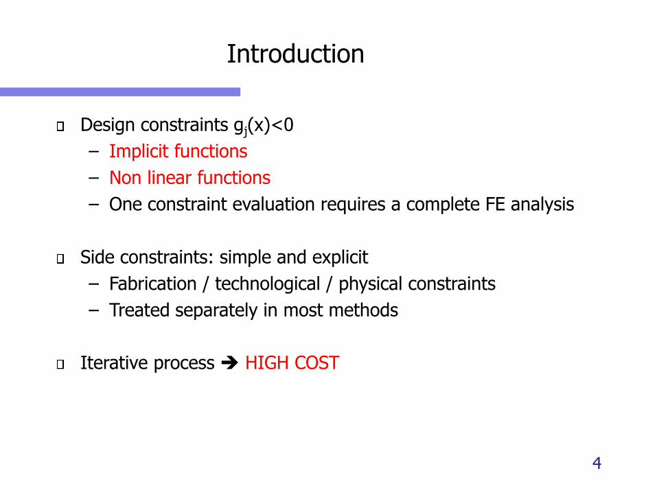
Design constraints gj(x)<0

– Implicit functions

– Non linear functions

– One constraint evaluation requires a complete FE analysis

Side constraints: simple and explicit

– Fabrication / technological / physical constraints

– Treated separately in most methods

Iterative process ➔ HIGH COST

4

INTRODUCTION

Optimality criteria techniques (OC)

– Highly specific

– Intuitive techniques, simple

– Convergence to a design that is not necessarily optimal (KKT conditions)

– Difficulties in identifying the set of active constraints

– Convergence instabilities

– Small number of reanalyses, independent of the number of design variables

Résumé

– Low cost

– But uncertainty convergence

5

INTRODUCTION

Pure Mathematical Programming methods

– Very general

– Rigorous methods, quite elaborated

– Convergence to a local minimum

– Stable and monotonic convergence

– Large number of reanalyses, growing with the number of design variables

Résumé

– Rigorous framework & guaranteed convergence

– High cost (Growing with the size of the problem)

6

BERKE’S APPROXIMATION

7

BERKE’S APPROXIMATION

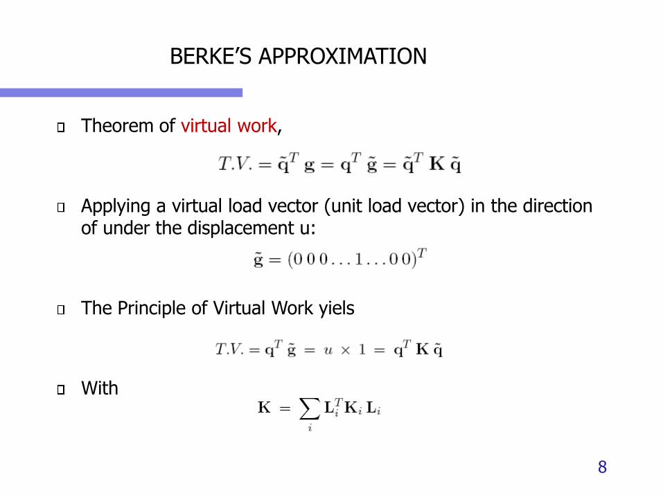
Theorem of virtual work,

Applying a virtual load vector (unit load vector) in the direction of under the displacement u:

The Principle of Virtual Work yiels

With

8

BERKE’S APPROXIMATION

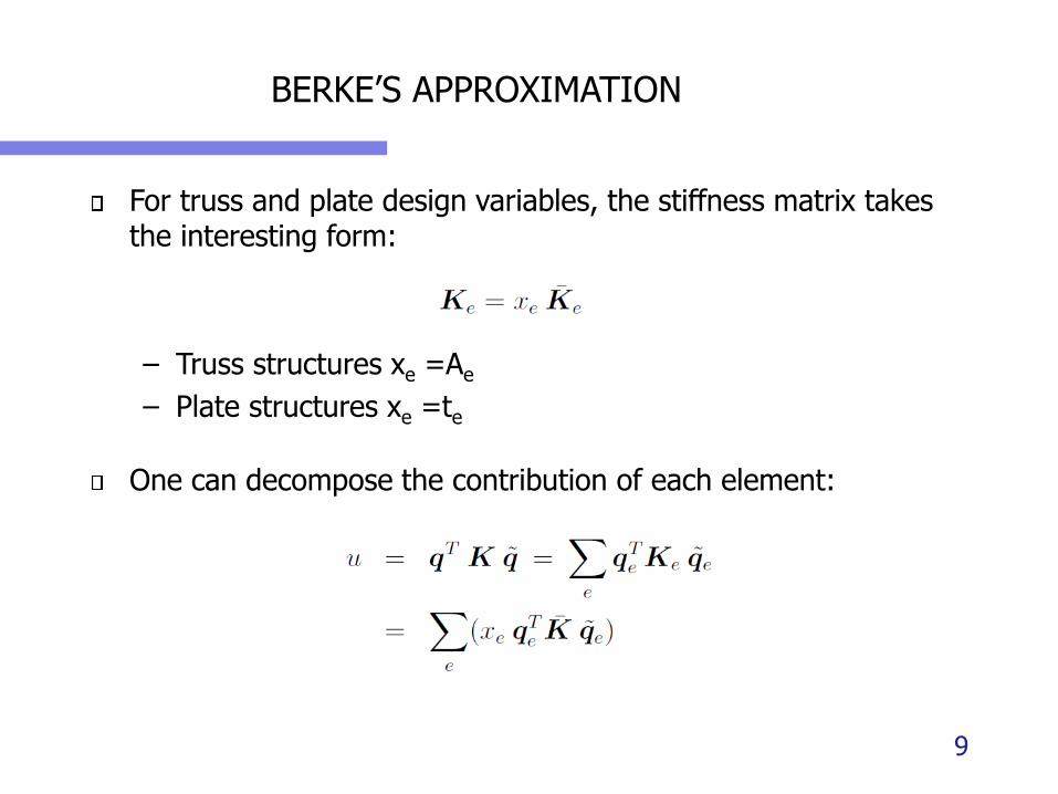
For truss and plate design variables, the stiffness matrix takes the interesting form:

– Truss structures xe =Ae

– Plate structures xe =te

One can decompose the contribution of each element:

9

BERKE’S APPROXIMATION

▪ The flexibility coefficients are constant for statically determinate structures

▪ For other structures, one can also assume a moderate redistribution of the internal loads around the current design point and has also constant value.

▪ Considering that the coefficients ce are constant, Berke'scriterion provides an explicit expression of the displacement u in terms of the design variables

10

BERKE’S APPROXIMATIONARE FIRST ORDER APPROXIMATIONS

11

A first order explicit approximation of displacement

▪ The Berke’s expansion provide a first order explicit approximation of the displacement around x0

▪ In general (indeterminate structures) the ci0 are not

constant

▪ The expression is exact for statically determinate structures, but for statically indeterminate structures, it is only exact in the current point x0

▪ The Berke’s expression is an approximation of the displacement u around the current design point x0 in terms of the design variables. 12

A first order explicit approximation of displacement

▪ The value of the approximation is exact in xi0

▪ As ci0 remains constant only along D(x0). It is also true for

all points along the scaling line

▪ The derivatives of the approximations are exact in xi0

13

APPROXIMATION IS A FIRST ORDER TAYLOR EXPANSION

IN THE RECIPROCAL VARIABLE SPACE

14

Constraint linearization in reciprocal space

▪ Berke’s approximation of the displacement u.

▪ Suggest to use the reciprocal variables

▪ The Berke’s approximation can take the simple form

15

Constraint linearization in reciprocal space

▪ We now show that the Berke’s approximation is in fact the first order Taylor expansion of the displacement in the reciprocal space.

▪ In order to prove that one has to show that

▪ Cij are the derivative of u with respect to zi:

▪ The constant terms in ‘0’ cancel each other

16

▪ It comes

▪ Finally

Constraint linearization in reciprocal space

17

0

Constraint linearization in reciprocal space

▪ Let’s show that the virtual energy densities ci are the first derivatives (gradients) of the constraints with respect to the reciprocal variables zi=1/xi that is

▪ For the approximation obviously, we have :

18

Constraint linearization in reciprocal space

▪ Derivative of the (real) displacement with respect to the reciprocal design variable zi = 1/xi. It is clear that

▪ Since

▪ It comes

19

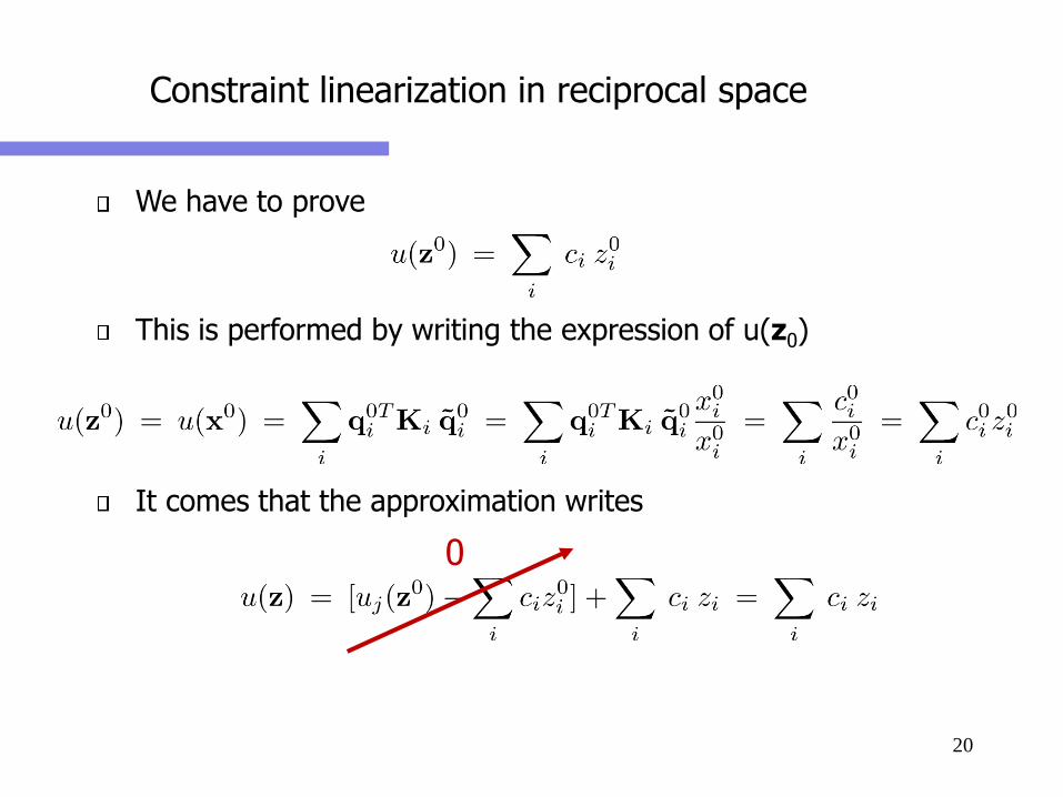
Constraint linearization in reciprocal space

We have to prove

This is performed by writing the expression of u(z0)

It comes that the approximation writes

20

0

First order explicit approximation of the stress constraints

Previous interpretation of FSD and Berke’s approximation suggests to generalize the first order approximation approach and to build the same high-quality approximations for stress and displacement constraints.

For truss: stress constraints can be equivalent to relative displacements. But in general

Apply “virtual load case” tk

The first order generalized “Berke” approximation of the stress

21

First order explicit approximation of the stress constraints

Property:

First order approximation on the scaling line

22

Constraint linearization in reciprocal space

Approximation concept approach:

– Linearization of the stress constraints

– First order explicit approximation

Conventional OC: stress ratio formula

– Fully stressed design (FSD) philosophy

– Zero order approximation23

Constraint linearization in reciprocal space

24

Stress ratioing

25

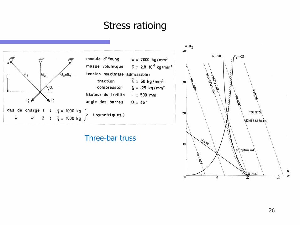
Stress ratioing

26

Three-bar truss

Stress ratioing

Direct design variables space27

Stress ratioing

28

Reciprocal design variables space

Stress ratioing

29

Stress ratioing

Three-bar truss:First order

approximation of stress constraints

30

RELATIONS BETWEEN OC AND MP

Generalized OC = MP linearization method

Approximation concept approach

Constraint gradients

31

Generalized OC = Linearization method

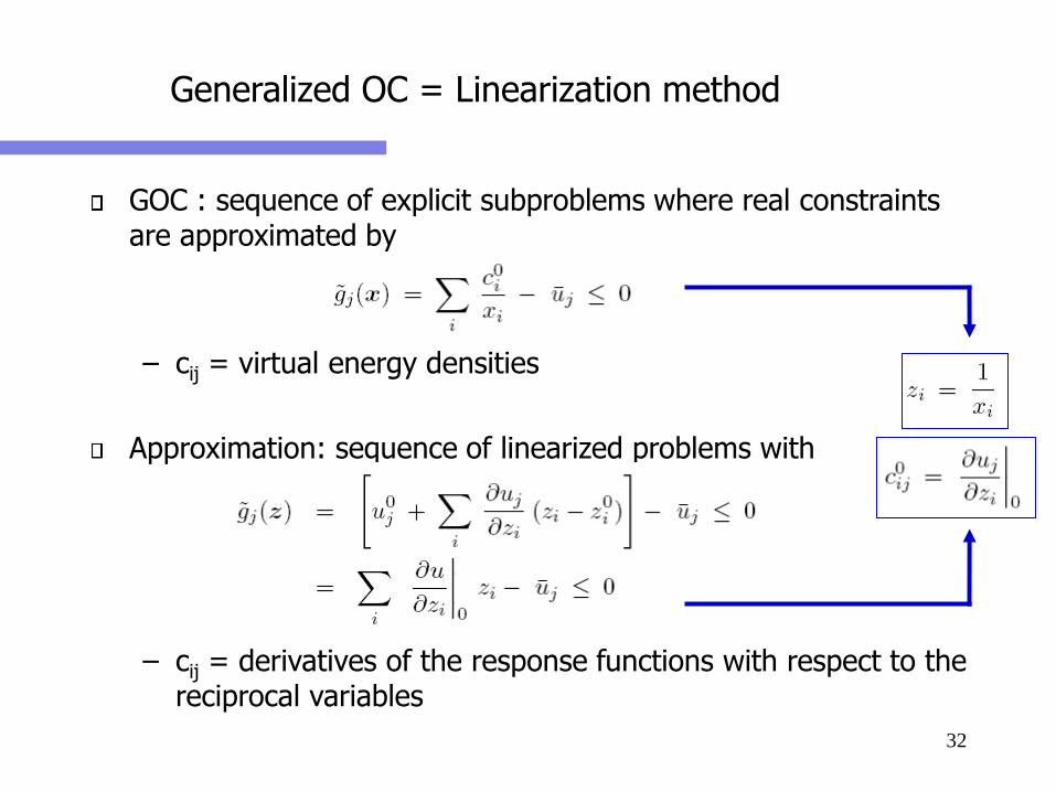
GOC : sequence of explicit subproblems where real constraints are approximated by

– cij = virtual energy densities

Approximation: sequence of linearized problems with

– cij = derivatives of the response functions with respect to the reciprocal variables

32

Generalized OC = Linearization method

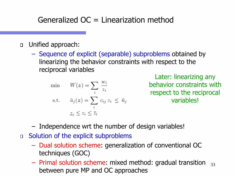
Unified approach:

– Sequence of explicit (separable) subproblems obtained by linearizing the behavior constraints with respect to the reciprocal variables

– Independence wrt the number of design variables!

Solution of the explicit subproblems

– Dual solution scheme: generalization of conventional OC techniques (GOC)

– Primal solution scheme: mixed method: gradual transition between pure MP and OC approaches

Later: linearizing any behavior constraints with respect to the reciprocal

variables!

33

CONCLUSION

34

CONCLUSION

▪ Berke’s approximation has been successful in providing high quality explicit approximations of displacement constraints

▪ Optimality Criteria can reduce substantially the number of function evaluation in solving costly problems in truss sizing

▪ They are used in building fast solution algorithms

▪ Berke’s approximations are first order Taylor expansion of the displacement in terms of the reciprocal design variables

▪ How can we extend the principle to other engineering design problems?

▪ Answer: Structural Approximations35

SEQUENTIAL CONVEX PROGRAMMING APPROACH

Direct solution of the original

optimisation problem which is

generally non-linear, implicit

in the design variables

is replaced by a sequence of optimisation sub-problems

by using approximations of the responses and using powerful

mathematical programming algorithms36

SEQUENTIAL CONVEX PROGRAMMING APPROACH

▪ Two basic concepts:

▪ Structural approximations replace the implicit problem by an

explicit optimisation sub-problem using convex, separable,

conservative approximations; e.g. CONLIN, MMA

▪ Solution of the convex sub-problems: efficient solution using dual

methods algorithms or SQP method.

▪ Advantages of SCP:

▪ Optimised design reached in a reduced number of iterations: 10 to

20 F.E. analyses

▪ Efficiency, robustness, generality, and flexibility, small computation

time

▪ Large scale problems in terms of number of design constraints and

variables 37