Embed Size (px)
Citation preview
Set-Valued Anal (2007) 15:139–162DOI 10.1007/s11228-006-0033-5
Optimality Conditions for Disjunctive Programswith Application to Mathematical Programswith Equilibrium Constraints
Michael L. Flegel · Christian Kanzow · Jirí V. Outrata
Received: 6 July 2005 / Accepted: 19 September 2006 /Published online: 15 December 2006© Springer Science + Business Media B.V. 2006
Abstract We consider optimization problems with a disjunctive structure of thefeasible set. Using Guignard-type constraint qualifications for these optimizationproblems and exploiting some results for the limiting normal cone by Mordukhovich,we derive different optimality conditions. Furthermore, we specialize these results tomathematical programs with equilibrium constraints. In particular, we show that anew constraint qualification, weaker than any other constraint qualification used inthe literature, is enough in order to show that a local minimum results in a so-calledM-stationary point. Additional assumptions are also discussed which guarantee thatsuch an M-stationary point is in fact a strongly stationary point.
Key words disjunctive programs · mathematical programs with equilibriumconstraints · M-stationarity · strong stationarity · Guignard constraint qualification.
Mathematics Subject Classifications (2000) 90C30 · 90C46
1 Introduction
In the past decade applied mathematicians have been paying increasing interest tooptimization problems where, among the constraints, so-called equilibrium con-straints occur. This equilibrium is described mostly by a (lower-level) optimization
M. L. Flegel (B) · C. KanzowInstitute of Mathematics, University of Würzburg, Am Hubland, 97074 Würzburg, Germanye-mail: [email protected]
C. Kanzowe-mail: [email protected]
J. V. OutrataAcademy of Sciences, Institute of Information Theory and Automation,18208 Prague, Czech Republice-mail: [email protected]
140 Set-Valued Anal (2007) 15:139–162
problem, a variational inequality or a complementarity problem. Following [13],all these problems are currently termed mathematical programs with equilibriumconstraints, or MPECs. Most of them can be written down in form of (smooth)nonlinear programs which, however, do not satisfy most of the standard constraintqualifications (CQs). This has lead to several weakened stationarity notions that havebeen introduced in connection with optimality conditions and numerical approaches.
Among these new stationarity notions an important role is played by a con-cept associated with the generalized differential calculus of Mordukhovich, cf.[16, 17, 28, 30]. Following [22], we will call it M-stationarity. The advantage of thisconcept consists, above all, in the fact that it requires only very weak constraintqualifications, cf. [5, 29]. Simultaneously, starting with [13], another, stronger, sta-tionarity notion has been investigated [18, 24, 27], referred to by the moniker strongstationarity in [22]. Strong stationarity is the natural candidate for a stationarityconcept for MPECs, because it is equivalent to the standard Karush–Kuhn–Tucker(KKT) conditions if the MPEC can be expressed as a standard nonlinear program. Asmentioned above, however, this stationarity concept is too restrictive in the contextof MPECs.
In this paper we will investigate the above mentioned stationarity notions bymeans of a general disjunctive program which embeds most MPECs considered inthe literature so far. In particular, we will show that local minimizers are M-stationaryunder an appropriate variant of the Guignard CQ [8], known to be the weakest CQused in classical nonlinear programming. Moreover, we will derive a new conditionwhich, together with this variant of Guignard CQ, ensures the strong stationarity oflocal minimizers. Our disjunctive structure is not induced by integral variables like,e.g., in [11]. It is also not related to a family of convex programs like the disjunctiveprogram investigated in [2].
Finally, these results will then be translated to the language of MPECs where theconstraints are described by a complementarity problem. In particular, we will showthat M- and strong stationarity indeed amount to the well-known conditions commonin the literature of these programs. Additionally, a new constraint qualification isintroduced to such MPECs by transferring the variant of Guignard CQ for ourdisjunctive programs to an MPEC setting. This yields the weakest result known todate, M-stationarity as a first order condition under this very weak CQ.
The organization of the paper is as follows. Section 2 is devoted to some prelimi-nary results including important definitions and some initial observations. The mainresults for the disjunctive program are collected in Section 3. Finally, in Section 4, weapply the results of Section 3 to a standard MPEC, where the equilibrium is modelledby a nonlinear complementarity problem. We then close with some final remarks inSection 5.
Our notation is standard. The n-dimensional Euclidean space is denoted by Rn,
its nonnegative and nonpositive orthant by Rn+ and R
n−, respectively. If unclear fromcontext, the size of a zero vector is denoted by an appropriate subscript: 0n is the zerovector in R
n. Given a vector x ∈ Rn, its components are denoted by xi. Furthermore,
given an index set ω ⊆ {1, . . . , n}, we denote by xω ∈ R|ω| the vector consisting of
those components xi corresponding to the indices in ω. The same terminology appliesto functions. Given a function F : R
n → Rm, we denote its Jacobian by ∇F(z) ∈
Rm×n. If m = 1, the gradient ∇F(z) ∈ R
n is considered a column vector. We calla set valued function a multifunction. Given such a multifunction �: R
p ⇒ Rq, its
Set-Valued Anal (2007) 15:139–162 141
graph is defined by gph � := {(u, v) ∈ Rp+q | v ∈ �(u)}. Finally, given an arbitrary
set K ⊆ Rn, it’s polar is defined by K◦ := {v ∈ R
n | vTw � 0 ∀w ∈ K}.
2 Preliminaries
For the reader’s convenience we start with the definitions of several basic notions invariational analysis which will be extensively used throughout the paper.
Let A ⊆ Rn be an arbitrary closed set and u ∈ A. The nonempty cone
TA(u) := lim supτ↘0
A − uτ
:={
d ∈ Rn | ∃{uk} ⊂ A, ∃{τk} ↘ 0 : uk → u,
uk − uτk
→ d}
is called the contingent (also Bouligand or tangent) cone to A at u. Consider thefamily of closed sets Ai, i = 1, . . . , k, and a point u ∈ ⋂k
i=1 Ai. Then it follows directlyfrom the above definition that
T⋃ki=1Ai
(u) =k⋃
i=1
TAi(u). (1)
Furthermore, we use the contingent cone to define the Fréchet normal cone
NA(u) := (TA(u))◦ (2)
to A at u. Note that the Fréchet normal cone is sometimes referred to as the regularnormal cone. This is most notably the case in [21]. Again, if we consider the familyof closed sets Ai, i = 1, . . . , k, and a point u ∈ ⋂k
i=1 Ai, it follows from Eq. 1 and theproperties of the polar cone that
N⋃ki=1 Ai
(u) = (T⋃k
i=1 Ai(u))◦ =
k⋂i=1
(TAi(u))◦ =k⋂
i=1
NAi(u) (3)
(see [1, Theorem 3.1.9]).The cornerstone of the generalized differential calculus of Mordukhovich is the
limiting normal cone, also called the Mordukhovich normal cone, defined by
NA(u) := lim supu′ A→u
NA(u′)
:={
limk→∞
wk | ∃{uk} ⊂ A : limk→∞
uk = u, wk ∈ NA(uk)
}.
In contrast to the Fréchet normal cone, NA(u) can be nonconvex, but admits awidely developed calculus, cf. [14, 21]. In this calculus, an important role is playedby stability of multifunctions reflecting the local structure of A. This will becomeimportant when we introduce constraint qualifications further down. Note that ifNA(u) = NA(u), we say that the set A is (normally) regular at u.
142 Set-Valued Anal (2007) 15:139–162
Consider now the general mathematical program
minimize f (z)
subject to F(z) ∈ �,(4)
where f : Rn→R, F: R
n→Rm are continuously differentiable functions and � ⊆ R
m
is a nonempty closed (possibly nonconvex) set. It is clear that the constraint F(z) ∈ �
can also incorporate geometric constraints of the form z ∈ �, where � ⊆ Rn is an
arbitrary closed set.Utilizing the normal cones introduced above, we are now able to define two
stationarity concepts which will play a central role in this paper.
Definition 1 Let z be feasible for the program (4).
(a) We say that z is M-stationary if there exists a KKT vector λ ∈ N�
(F(z)
)such
that
0 = ∇ f (z) + (∇F(z))T
λ. (5)
(b) We say that z is strongly stationary if (5) is fulfilled with a KKT vector λ ∈N�(F(z)).
Note that M- and strong stationarity may be expressed as
0 ∈ ∇ f (z) + (∇F(z))T
N�
(F(z)
)and
0 ∈ ∇ f (z) + (∇F(z))T
N�
(F(z)
),
respectively.The name M-stationarity is motivated by the fact that it involves the Mordukh-
ovich normal cone. It was coined in the context of MPECs by Scholtes [23]. Similarly,we use the name strong stationarity in accordance with [22], where it was also usedin the context of MPECs. In the MPEC setting, strong stationarity is sometimes alsoreferred to as primal-dual stationarity [18].
As already mentioned, M-stationarity is a weaker stationarity concept than strongstationarity. However, the limiting normal cone (though nonconvex in general) hasan extensive calculus, whereas the fuzzy calculus, developed for the Fréchet normalcone does not seem useful for our purposes.
Having introduced stationarity concepts for the program (4), we now turn ourattention to constraint qualifications. To this end, we need the concept of calmnessof multifunctions and the closely related idea of upper Lipschitz continuity.
Definition 2 Let �: Rp ⇒ R
q be a multifunction with a closed graph and (u, v) ∈gph �. We say that � is calm at (u, v) provided there exist neighborhoods U of u, Vof v, and a modulus L � 0 such that
�(u′) ∩ V ⊂ �(u) + L‖u′ − u‖ B for all u′ ∈ U . (6)
If Eq. 6 holds true with V = Rq, � is said to be locally upper Lipschitz continuous at
u, cf. [20].
Set-Valued Anal (2007) 15:139–162 143
Note that calmness is sometimes also referred to as pseudo upper Lipschitzcontinuity (see, e.g., [30]) and that in [21] both calmness and local upper Lipschitzcontinuity are referred to as calmness.
To obtain a constraint qualification for the program (4), we define a multifunctionM: R
m ⇒ Rn associated with the constraint system of Eq. 4 in the following fashion:
M(p) := {z ∈ R
n | F(z) + p ∈ �}. (7)
We can now use this multifunction to define a constraint qualification under which M-stationarity is a first order optimality condition. This is made precise in the followingtheorem, a proof of which may be found, e.g., in [17, Theorem 2.4].
Theorem 3 Let z be a local minimizer of the program (4). If the multifunction M (seeEq. 7) is calm at (0, z), z is M-stationary.
Note that if we drop the continuous differentiability of f and F in favor ofLipschitz continuity near z of these functions, the result of Theorem 3 remains trueif we state M-stationarity (5) in terms of the subgradient of f and the coderivative ofan appropriate function, see [30] for details.
A constraint qualification better known in nonlinear programming is theMangasarian–Fromovitz constraint qualification (MFCQ). We define a generaliza-tion of this CQ.
Definition 4 Let z be feasible for the program (4). We say that the general-ized Mangasarian–Fromovitz constraint qualification (GMFCQ) holds at z if theimplication
∇F(z)Tλ = 0
λ ∈ N�
(F(z)
)}
=⇒ λ = 0 (8)
holds.
If � = Rm− , the condition (8) reduces to the classical Mangasarian–Fromovitz
constraint qualification, justifying the name GMFCQ.We now show that M-stationarity is a first order condition under GMFCQ.
Corollary 5 Let z be a local minimizer of the program (4) at which GMFCQ holds.Then z is M-stationary.
Proof Due to Theorem 3, it suffices to show that GMFCQ implies the calmness of Mat (0, z). From [15, Corollary 4.4], we readily infer that GMFCQ implies the so-calledAubin property of M around (0, z). Since this property is stronger than the requiredcalmness (see, e.g., [21, Definition 9.36]), the result follows. ��
For more information on the Aubin property, we refer the reader to the book byRockafellar and Wets [21].
Having discussed both calmness and GMFCQ as constraint qualifications, wenow introduce generalizations of the Abadie and Guignard constraint qualificationsknown from standard nonlinear programming.
144 Set-Valued Anal (2007) 15:139–162
Definition 6 Let z be feasible for the program (4).
(a) We say that the generalized Abadie constraint qualification (GACQ) holds at zif
TF−1(�)(z) = L(z), (9)
where
L(z) := {h ∈ R
n | ∇F(z) h ∈ T�
(F(z)
)}(10)
is called the linearized cone at z.(b) We say that the generalized (or dual) Guignard constraint qualification
(GGCQ) holds at z if
NF−1(�)(z) = (L(z)
)◦. (11)
To justify the names of the above constraint qualifications, we apply them to astandard nonlinear program that takes the form
minimize f (z)
subject to g(z) � 0, h(z) = 0, (12)
with continuously differentiable f : Rn → R, g: R
n → Rm, and h: R
n → Rp. To for-
mulate this program in the fashion of the program (4), we set
F(z) := (g(z), h(z)) and � := Rm− × 0p.
It is then easily verified that
L(z) = {d ∈ Rn | ∇gi(z)Td � 0, ∀i ∈ Ig,
∇hi(z)Td = 0, ∀i = 1, . . . , p },where Ig := {i | gi(z) = 0} is the set of active inequality constraints.
Clearly, in this case GACQ and GGCQ reduce to the standard definitions ofAbadie and Guignard CQ, respectively, as they are most commonly stated, see,e.g., [1]. However, Guignard [8] originally stated her CQ in the primal form. Herdefinition is equivalent to the above dual characterization of Guignard CQ if �
is convex. In the nonconvex case the relationship is not as straightforward. SinceGuignard CQ is commonly defined using the dual formulation (see, e.g., [1, 7, 19, 25]),however, we feel justified in calling Eq. 11 the generalized Guignard CQ.
Note that since NF−1(�)(z) = TF−1(�)(z)◦ by definition (see Eq. 2), GACQ at zobviously implies GGCQ at z. Furthermore, as proved in [10, Proposition 1],calmness of M at (0, z) implies GACQ at z. This yields the following chain ofimplications:
calmness of M at (0, z) =⇒ GACQ at z =⇒ GGCQ at z, (13)
where calmness of M at (0, z) is implied either by GMFCQ at z or by the upperLipschitz continuity of M at z. Therefore, due to [20, Proposition 1], M is calm at(0, z), whenever F is affine and � is polyhedral.
In general, none of the above implications can be reversed.
Set-Valued Anal (2007) 15:139–162 145
An important question surrounding GACQ and GGCQ is their connection withoptimality conditions. It is known that if � is convex, strong stationarity is a first orderoptimality condition under GGCQ and hence under GACQ (see the argumentsfollowing Definition 6). In the following sections we will investigate how this canbe extended to nonconvex �.
Another question is when we might expect strong stationarity to be a first orderoptimality condition. Since f is continuously differentiable, we have the well-knownoptimality condition
0 ∈ ∇ f (z) + NF−1(�)(z), (14)
cf., e.g., [21, Theorem 6.12]. Unfortunately, we only have the inclusion
NF−1(�)(z) ⊃ (∇F(z))T
N�
(F(z)
)(15)
which turns out to be an equality provided GMFCQ is satisfied at z and � is(normally) regular at F(z) (see [21, Theorem 6.14]). However, this condition neverholds for equilibrium constraints. This question is important, because we needto have equality in the inclusion (15) in order to explicitly determine the coneNF−1(�)(z), and with it to be able to verify whether strong stationarity holds.
3 The Disjunctive Program
In this section we will investigate GACQ and GGCQ in context with M- and strongstationarity under the structural assumption that
� =k⋃
i=1
�i, (16)
where all �i, i = 1, . . . , k, are convex polyhedra. This assumption is satisfied by alarge class of equilibrium constraints, see Section 4 for an example of this.
The sets �i are called components and with each z ∈ � we associate the index setI(z) of active components defined by
I(z) := {i ∈ {1, . . . , k} | F(z) ∈ �i} .
For the remainder of this section, we will confine ourselves to the program
minimize f (z)
subject toF(z) ∈ � =⋃k
i=1�i. (17)
For such a program, we are indeed able to show that M-stationarity is a necessaryfirst order condition under GGCQ and hence GACQ.
Theorem 7 Let z be a local minimizer of the program (17). Then, if GGCQ is satisfiedat z, z is M-stationary.
Proof As mentioned in the previous section, relation (14) holds true. Thus, due toGGCQ at z, one has
0 ∈ ∇ f (z) + (L(z)
)◦. (18)
146 Set-Valued Anal (2007) 15:139–162
By definition of the polar cone, this means that h = 0 is the (unique) solution of theprogram
minimize ∇ f (z)T hsubject to ∇F(z) h ∈ T�
(F(z)
). (19)
By virtue of Eq. 1,
T�
(F(z)
) =⋃
i∈I(z)
T�i
(F(z)
).
Consider now the multifunction M: Rm ⇒ R
n, defined by
M(p) := {h ∈ R
n | ∇F(z) h + p ∈ T�
(F(z)
)}.
Clearly, the constraint in the program (19) can equivalently be written as h ∈ M(0).Moreover, since the contingent cones T�i
(F(z)
), i ∈ I(z), are convex polyhedra,
gph M =⎧⎨⎩(p, h) ∈ R
m × Rn | ∇F(z) h + p ∈
⋃i∈I(z)
T�i
(F(z)
)⎫⎬⎭
=⋃
i∈I(z)
{(p, h) ∈ R
m × Rn | ∇F(z) h + p ∈ T�i
(F(z)
)}
is a union of finitely many convex polyhedra (the second equality is trivially verified).From [20, Proposition 1] it follows that M is locally upper Lipschitz at 0 and, afortiori, calm at (0, z). Thus, by [9, Theorem 4.1] we have
NM(0)(0) ⊆ (∇F(z))T
NT�(F(z))(0). (20)
It remains to invoke [21, Example 6.47] according to which, due to Eq. 1, there existsa neighborhood O of F(z) in R
m such that
� ∩ O = [F(z) + T�
(F(z)
)] ∩ O.
Consequently, by the definition of the limiting normal cone,
NT�(F(z))(0) = NF(z)+T�(F(z))
(F(z)
) = N�
(F(z)
). (21)
Finally, remembering that h = 0 is a minimizer of the program (19), applying theoptimality condition (14) to the program (19) yields (note that h is the variable)
0(14)∈ ∇ f (z) + NM(0)(0)
⊆ ∇ f (z) + NM(0)(0)
(20)⊆ ∇ f (z) + (∇F(z))T
NT�(F(z))(0)
(21)= ∇ f (z) + (∇F(z))T
N�
(F(z)
).
This is the condition for M-stationarity (5), completing the proof. ��
Set-Valued Anal (2007) 15:139–162 147
Note that the continuous differentiability of f enters crucially in constructingthe program (19). The statement of Theorem 7 cannot be proved using the abovetechnique if we replace continuously differentiable data with locally Lipschitz data.
We now turn our attention to strong stationarity of z if it is a minimizer of aprogram (17). Let us consider the following academic example, taken from [27].
Example 8 Consider the program
minimize −z2
subject to
⎡⎣ z1
z2
z1 − z2
⎤⎦ ∈ �1 ∪ �2,
with �1 = R+ × {0} × {0} and �2 = {0} × R+ × {0}. It is easy to verify that z = 0 isthe unique minimizer of this program and that GMFCQ is satisfied at the origin.Hence, z is M-stationary and the vector
λ =⎡⎣ 0
10
⎤⎦ ∈ N�(0) (22)
belongs to the set of KKT vectors. On the other hand,
N�(0) = N�1(0) ∩ N�2(0) = {λ ∈ R
3 | λ1 � 0, λ2 � 0}
(see Eq. 3) and we easily verify that there exists no λ = (λ1, λ2, λ3) ∈ N�(0) such that
0 ∈[
0−1
]+[
1 0 10 1 −1
]⎡⎣ λ1
λ2
λ3
⎤⎦ .
This example shows (by virtue of Eq. 13) that none of the CQs mentioned inSection 2 can ensure strong stationarity of local minima in the considered program.We therefore need an additional condition which we introduce in the followingdefinition.
Definition 9 Let z be feasible for the program (17). We say that the intersectionproperty holds at z if
⋂i∈I(z)
(∇F(z))T
N�i
(F(z)
) = (∇F(z))T ⋂
i∈I(z)
N�i
(F(z)
). (I)
In order to use the intersection property to acquire a stronger optimality condi-tion, we first need the following result, concerning the polar of a polyhedral cone, theproof of which may be found in [1, Theorem 3.2.2].
Lemma 10 Let the cones
K1 := {d ∈ Rn | aT
i d � 0, ∀i = 1, . . . , k,
bTj d = 0, ∀ j = 1, . . . , l} (23)
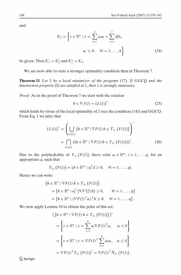
148 Set-Valued Anal (2007) 15:139–162
and
K2 ={v ∈ R
n | v =k∑
i=1
αiai +l∑
j=1
βjbj,
αi � 0, ∀i = 1, . . . , k}
(24)
be given. Then K1 = K◦2 and K◦
1 = K2.
We are now able to state a stronger optimality condition than in Theorem 7.
Theorem 11 Let z be a local minimizer of the program (17). If GGCQ and theintersection property (I) are satisfied at z, then z is strongly stationary.
Proof As in the proof of Theorem 7 we start with the relation
0 ∈ ∇ f (z) + (L(z)
)◦ (25)
which holds by virtue of the local optimality of z (see the condition (14)) and GGCQ.From Eq. 1 we infer that
(L(z)
)◦ =⎛⎝⋃
i∈I(z)
{h ∈ R
n | ∇F(z) h ∈ T�i
(F(z)
)}⎞⎠
◦
=⋂
i∈I(z)
({h ∈ Rn | ∇F(z) h ∈ T�i
(F(z)
)})◦. (26)
Due to the polyhedrality of T�i
(F(z)
), there exist ai ∈ R
m, i = 1, . . . , q, for anappropriate q, such that
T�i
(F(z)
) = {d ∈ Rm | aT
i d � 0, ∀i = 1, . . . , q}.Hence we can write
{h ∈ R
n | ∇F(z) h ∈ T�i
(F(z)
)}= {
h ∈ Rn | aT
i
(∇F(z)
h)� 0, ∀i = 1, . . . , q
}= {
h ∈ Rn | (∇F(z)Tai)
T h � 0, ∀i = 1, . . . , q}.
We now apply Lemma 10 to obtain the polar of this set:( {
h ∈ Rn | ∇F(z) h ∈ T�i
(F(z)
)} )◦
={
v ∈ Rn | v =
q∑i=1
αi∇F(z)Tai, α � 0
}
={
v ∈ Rn | v = ∇F(z)T
q∑i=1
αiai, α � 0
}
= ∇F(z)T T�i
(F(z)
)◦ = ∇F(z)T N�i
(F(z)
),
Set-Valued Anal (2007) 15:139–162 149
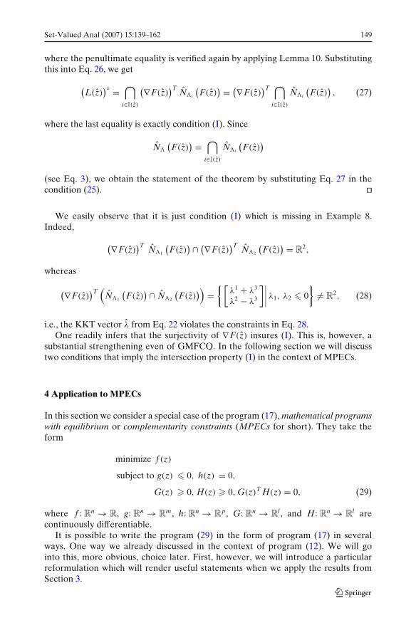
where the penultimate equality is verified again by applying Lemma 10. Substitutingthis into Eq. 26, we get
(L(z)
)◦ =⋂
i∈I(z)
(∇F(z))T
N�i
(F(z)
) = (∇F(z))T ⋂
i∈I(z)
N�i
(F(z)
), (27)
where the last equality is exactly condition (I). Since
N�
(F(z)
) =⋂
i∈I(z)
N�i
(F(z)
)
(see Eq. 3), we obtain the statement of the theorem by substituting Eq. 27 in thecondition (25). ��
We easily observe that it is just condition (I) which is missing in Example 8.Indeed,
(∇F(z))T
N�1
(F(z)
) ∩ (∇F(z))T
N�2
(F(z)
) = R2,
whereas
(∇F(z))T(
N�1
(F(z)
) ∩ N�2
(F(z)
)) ={[
λ1 + λ3
λ2 − λ3
]∣∣∣∣ λ1, λ2 � 0
}�= R
2, (28)
i.e., the KKT vector λ from Eq. 22 violates the constraints in Eq. 28.One readily infers that the surjectivity of ∇F(z) insures (I). This is, however, a
substantial strengthening even of GMFCQ. In the following section we will discusstwo conditions that imply the intersection property (I) in the context of MPECs.
4 Application to MPECs
In this section we consider a special case of the program (17), mathematical programswith equilibrium or complementarity constraints (MPECs for short). They take theform
minimize f (z)
subject to g(z) � 0, h(z) = 0,
G(z) � 0, H(z) � 0, G(z)T H(z) = 0, (29)
where f : Rn → R, g: R
n → Rm, h: R
n → Rp, G: R
n → Rl , and H: R
n → Rl are
continuously differentiable.It is possible to write the program (29) in the form of program (17) in several
ways. One way we already discussed in the context of program (12). We will gointo this, more obvious, choice later. First, however, we will introduce a particularreformulation which will render useful statements when we apply the results fromSection 3.
150 Set-Valued Anal (2007) 15:139–162
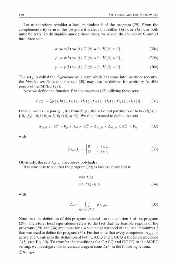
Let us therefore consider a local minimizer z of the program (29). From thecomplementarity term in this program it is clear that either Gi(z), or Hi(z), or bothmust be zero. To distinguish among these cases, we divide the indices of G and Hinto three sets:
α := α(z) := {i | Gi(z) = 0, Hi(z) > 0
}, (30a)
β := β(z) := {i | Gi(z) = 0, Hi(z) = 0
}, (30b)
γ := γ (z) := {i | Gi(z) > 0, Hi(z) = 0
}. (30c)
The set β is called the degenerate or, a term which has come into use more recently,the biactive set. Note that the sets (30) may also be defined for arbitrary feasiblepoints of the MPEC (29).
Next we define the function F in the program (17) utilizing these sets:
F(z) := (g(z), h(z), Gα(z), Hα(z), Gβ(z), Hβ(z), Gγ (z), Hγ (z)
). (31)
Finally, we take a pair (β1, β2) from P(β), the set of all partitions of beta (P(β) :={(β1, β2) | β1 ∪ β2 = β, β1 ∩ β2 = ∅}). We then proceed to define the sets
�β1,β2 := Rm− × 0p × 0|α| × R
|α|+ × �β1,β2 × �β2,β1 × R
|γ |+ × 0|γ | (32)
with
(�μ,ν
)j :=
{0 : j ∈ μ
R+ : j ∈ ν.(33)
Obviously, the sets �β1,β2 are convex polyhedra.It is now easy to see that the program (29) is locally equivalent to
min f (z)
s.t. F(z) ∈ � (34)
with
� :=⋃
(β1,β2)∈P(β)
�β1,β2 . (35)
Note that the definition of this program depends on the solution z of the program(29). Therefore, local equivalence refers to the fact that the feasible regions of theprograms (29) and (34) are equal for a whole neighborhood of the local minimizer zthat was used to define the program (34). Further note that every component �β1,β2 isactive at z. Central to the definition of both GACQ and GGCQ is the linearized coneL(z) (see Eq. 10). To transfer the conditions for GACQ and GGCQ to the MPECsetting, we investigate this linearized tangent cone L(z) in the following lemma.
Set-Valued Anal (2007) 15:139–162 151
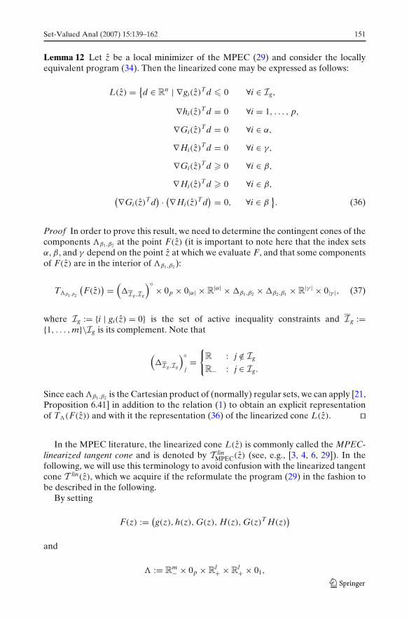
Lemma 12 Let z be a local minimizer of the MPEC (29) and consider the locallyequivalent program (34). Then the linearized cone may be expressed as follows:
L(z) = {d ∈ R
n | ∇gi(z)Td � 0 ∀i ∈ Ig,
∇hi(z)Td = 0 ∀i = 1, . . . , p,
∇Gi(z)Td = 0 ∀i ∈ α,
∇ Hi(z)Td = 0 ∀i ∈ γ,
∇Gi(z)Td � 0 ∀i ∈ β,
∇ Hi(z)Td � 0 ∀i ∈ β,
(∇Gi(z)Td) · (∇ Hi(z)Td
) = 0, ∀i ∈ β}. (36)
Proof In order to prove this result, we need to determine the contingent cones of thecomponents �β1,β2 at the point F(z) (it is important to note here that the index setsα, β, and γ depend on the point z at which we evaluate F, and that some componentsof F(z) are in the interior of �β1,β2 ):
T�β1 ,β2
(F(z)
) =(�Ig,Ig
)◦ × 0p × 0|α| × R|α| × �β1,β2 × �β2,β1 × R
|γ | × 0|γ |, (37)
where Ig := {i | gi(z) = 0} is the set of active inequality constraints and Ig :={1, . . . , m}\Ig is its complement. Note that
(�Ig,Ig
)◦j={
R : j /∈ Ig
R− : j ∈ Ig.
Since each �β1,β2 is the Cartesian product of (normally) regular sets, we can apply [21,Proposition 6.41] in addition to the relation (1) to obtain an explicit representationof T�(F(z)) and with it the representation (36) of the linearized cone L(z). ��
In the MPEC literature, the linearized cone L(z) is commonly called the MPEC-linearized tangent cone and is denoted by T lin
MPEC(z) (see, e.g., [3, 4, 6, 29]). In thefollowing, we will use this terminology to avoid confusion with the linearized tangentcone T lin(z), which we acquire if the reformulate the program (29) in the fashion tobe described in the following.
By setting
F(z) := (g(z), h(z), G(z), H(z), G(z)T H(z)
)
and
� := Rm− × 0p × R
l+ × R
l+ × 01,
152 Set-Valued Anal (2007) 15:139–162
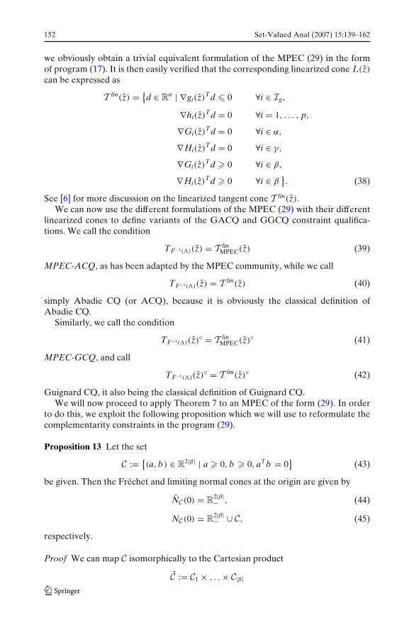
we obviously obtain a trivial equivalent formulation of the MPEC (29) in the formof program (17). It is then easily verified that the corresponding linearized cone L(z)
can be expressed as
T lin(z) = {d ∈ R
n | ∇gi(z)Td � 0 ∀i ∈ Ig,
∇hi(z)Td = 0 ∀i = 1, . . . , p,
∇Gi(z)Td = 0 ∀i ∈ α,
∇ Hi(z)Td = 0 ∀i ∈ γ,
∇Gi(z)Td � 0 ∀i ∈ β,
∇ Hi(z)Td � 0 ∀i ∈ β}. (38)
See [6] for more discussion on the linearized tangent cone T lin(z).We can now use the different formulations of the MPEC (29) with their different
linearized cones to define variants of the GACQ and GGCQ constraint qualifica-tions. We call the condition
TF−1(�)(z) = T linMPEC(z) (39)
MPEC-ACQ, as has been adapted by the MPEC community, while we call
TF−1(�)(z) = T lin(z) (40)
simply Abadie CQ (or ACQ), because it is obviously the classical definition ofAbadie CQ.
Similarly, we call the condition
TF−1(�)(z)◦ = T linMPEC(z)◦ (41)
MPEC-GCQ, and call
TF−1(�)(z)◦ = T lin(z)◦ (42)
Guignard CQ, it also being the classical definition of Guignard CQ.We will now proceed to apply Theorem 7 to an MPEC of the form (29). In order
to do this, we exploit the following proposition which we will use to reformulate thecomplementarity constraints in the program (29).
Proposition 13 Let the set
C := {(a, b) ∈ R
2|β| | a � 0, b � 0, aTb = 0}
(43)
be given. Then the Fréchet and limiting normal cones at the origin are given by
NC(0) = R2|β|− , (44)
NC(0) = R2|β|− ∪ C, (45)
respectively.
Proof We can map C isomorphically to the Cartesian product
C := C1 × . . . × C|β|
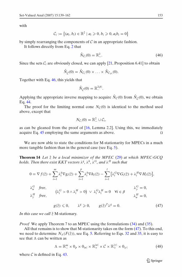
Set-Valued Anal (2007) 15:139–162 153
with
Ci := {(ai, bi) ∈ R
2 | ai � 0, bi � 0, aibi = 0}
by simply rearranging the components of C in an appropriate fashion.It follows directly from Eq. 2 that
NCi(0) = R2−. (46)
Since the sets Ci are obviously closed, we can apply [21, Proposition 6.41] to obtain
NC(0) = NC1(0) × . . . × NC|β|(0).
Together with Eq. 46, this yields that
NC(0) = R2|β|− .
Applying the appropriate inverse mapping to acquire NC(0) from NC(0), we obtainEq. 44.
The proof for the limiting normal cone NC(0) is identical to the method usedabove, except that
NCi(0) = R2− ∪ Ci,
as can be gleaned from the proof of [16, Lemma 2.2]. Using this, we immediatelyacquire Eq. 45 employing the same arguments as above. ��
We are now able to state the conditions for M-stationarity for MPECs in a muchmore tangible fashion than in the general case (see Eq. 5).
Theorem 14 Let z be a local minimizer of the MPEC (29) at which MPEC-GCQholds. Then there exist KKT vectors λg, λh, λG, and λH such that
0 = ∇ f (z) +m∑
i=1
λgi ∇gi(z) +
p∑i=1
λhi ∇hi(z) −
l∑i=1
[λG
i ∇Gi(z) + λHi ∇ Hi(z)
],
λGα free,
λHγ free,
(λG
i > 0 ∧ λHi > 0
) ∨ λGi λH
i = 0 ∀i ∈ βλG
γ = 0,
λHα = 0,
g(z) � 0, λg � 0, g(z)Tλg = 0. (47)
In this case we call z M-stationary.
Proof We apply Theorem 7 to an MPEC using the formulations (34) and (35).All that remains is to show that M-stationarity takes on the form (47). To this end,
we need to determine N�(F(z)), see Eq. 5. Referring to Eqs. 32 and 35, it is easy tosee that � can be written as
� = Rm− × 0p × 0|α| × R
|α|+ × C × R
|γ |+ × 0|γ | (48)
where C is defined in Eq. 43.
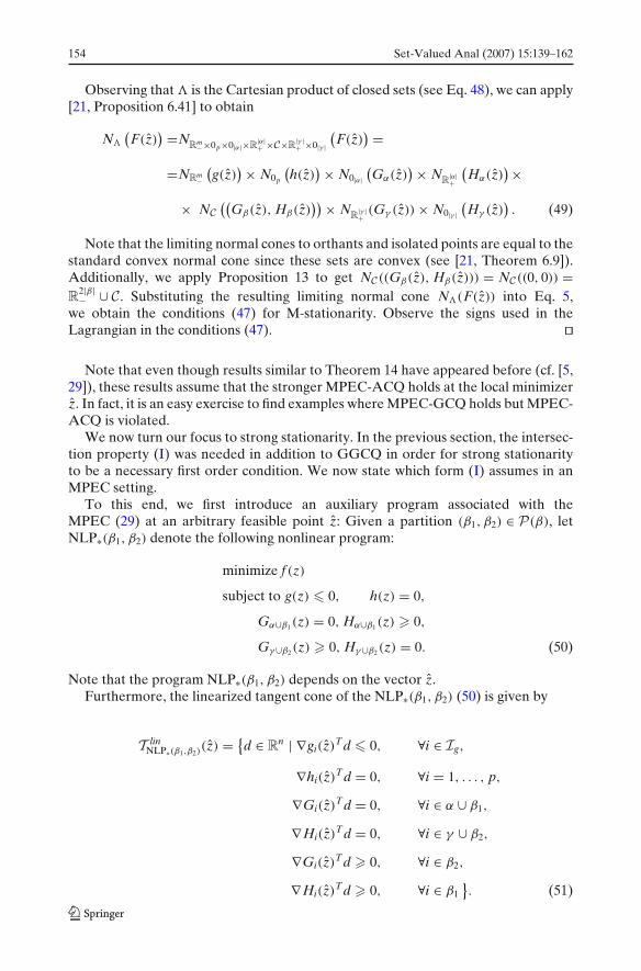
154 Set-Valued Anal (2007) 15:139–162
Observing that � is the Cartesian product of closed sets (see Eq. 48), we can apply[21, Proposition 6.41] to obtain
N�
(F(z)
) =NR
m−×0p×0|α|×R|α|+ ×C×R
|γ |+ ×0|γ |
(F(z)
) =
=NRm−(g(z)
)× N0p
(h(z)
)× N0|α|(Gα(z)
)× NR
|α|+
(Hα(z)
)×× NC
((Gβ(z), Hβ(z)
))× NR
|γ |+
(Gγ (z)) × N0|γ |(Hγ (z)
). (49)
Note that the limiting normal cones to orthants and isolated points are equal to thestandard convex normal cone since these sets are convex (see [21, Theorem 6.9]).Additionally, we apply Proposition 13 to get NC((Gβ(z), Hβ(z))) = NC((0, 0)) =R
2|β|− ∪ C. Substituting the resulting limiting normal cone N�(F(z)) into Eq. 5,
we obtain the conditions (47) for M-stationarity. Observe the signs used in theLagrangian in the conditions (47). ��
Note that even though results similar to Theorem 14 have appeared before (cf. [5,29]), these results assume that the stronger MPEC-ACQ holds at the local minimizerz. In fact, it is an easy exercise to find examples where MPEC-GCQ holds but MPEC-ACQ is violated.
We now turn our focus to strong stationarity. In the previous section, the intersec-tion property (I) was needed in addition to GGCQ in order for strong stationarityto be a necessary first order condition. We now state which form (I) assumes in anMPEC setting.
To this end, we first introduce an auxiliary program associated with theMPEC (29) at an arbitrary feasible point z: Given a partition (β1, β2) ∈ P(β), letNLP∗(β1, β2) denote the following nonlinear program:
minimize f (z)
subject to g(z) � 0, h(z) = 0,
Gα∪β1(z) = 0, Hα∪β1(z) � 0,
Gγ∪β2(z) � 0, Hγ∪β2(z) = 0. (50)
Note that the program NLP∗(β1, β2) depends on the vector z.Furthermore, the linearized tangent cone of the NLP∗(β1, β2) (50) is given by
T linNLP∗(β1,β2)
(z) = {d ∈ R
n | ∇gi(z)Td � 0, ∀i ∈ Ig,
∇hi(z)Td = 0, ∀i = 1, . . . , p,
∇Gi(z)Td = 0, ∀i ∈ α ∪ β1,
∇ Hi(z)Td = 0, ∀i ∈ γ ∪ β2,
∇Gi(z)Td � 0, ∀i ∈ β2,
∇ Hi(z)Td � 0, ∀i ∈ β1}. (51)
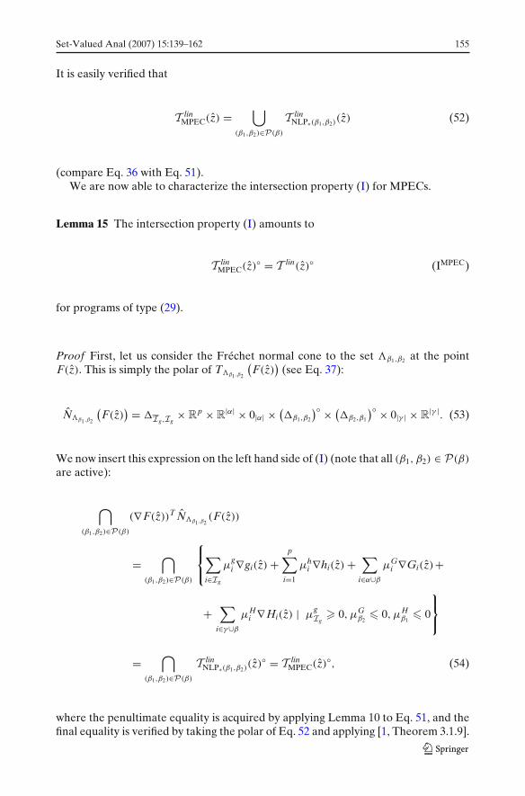
Set-Valued Anal (2007) 15:139–162 155
It is easily verified that
T linMPEC(z) =
⋃(β1,β2)∈P(β)
T linNLP∗(β1,β2)
(z) (52)
(compare Eq. 36 with Eq. 51).We are now able to characterize the intersection property (I) for MPECs.
Lemma 15 The intersection property (I) amounts to
T linMPEC(z)◦ = T lin(z)◦ (IMPEC)
for programs of type (29).
Proof First, let us consider the Fréchet normal cone to the set �β1,β2 at the pointF(z). This is simply the polar of T�β1 ,β2
(F(z)
)(see Eq. 37):
N�β1 ,β2
(F(z)
) = �Ig,Ig× R
p × R|α| × 0|α| × (
�β1,β2
)◦ × (�β2,β1
)◦ × 0|γ | × R|γ |. (53)
We now insert this expression on the left hand side of (I) (note that all (β1, β2) ∈ P(β)
are active):
⋂(β1,β2)∈P(β)
(∇F(z))T N�β1 ,β2(F(z))
=⋂
(β1,β2)∈P(β)
⎧⎨⎩∑i∈Ig
μgi ∇gi(z) +
p∑i=1
μhi ∇hi(z) +
∑i∈α∪β
μGi ∇Gi(z)+
+∑
i∈γ∪β
μHi ∇ Hi(z) | μ
gIg
� 0, μGβ2
� 0, μHβ1
� 0
⎫⎬⎭
=⋂
(β1,β2)∈P(β)
T linNLP∗(β1,β2)
(z)◦ = T linMPEC(z)◦, (54)
where the penultimate equality is acquired by applying Lemma 10 to Eq. 51, and thefinal equality is verified by taking the polar of Eq. 52 and applying [1, Theorem 3.1.9].
156 Set-Valued Anal (2007) 15:139–162
We now turn our attention to the right hand side of (I), again inserting Eq. 53:
(∇F(z))T⋂
(β1,β2)∈P(β)
N�β1 ,β2(F(z))
= (∇F(z))T{μ | μ ∈
⋂(β1,β2)∈P(β)
(�Ig,Ig
×Rp×R
|α|×0|α|×�◦β1,β2
×
× �◦β2,β1
× 0|γ |×R|γ |)}
= (∇F(z))T{μ | μ ∈ �Ig,Ig
× Rp × R
|α| × 0|α| × R|β|− × R
|β|− × 0|γ | × R
|γ |}
=⎧⎨⎩∑i∈Ig
μgi ∇gi(z) +
p∑i=1
μhi ∇hi(z) +
∑i∈α∪β
μGi ∇Gi(z) +
+∑
i∈γ∪β
μHi ∇ Hi(z) | μ
gIg
� 0, μGβ � 0, μH
β � 0
⎫⎬⎭
= T lin(z)◦. (55)
Again, the last equality is verified by applying Lemma 10 to Eq. 38.Finally, Eqs. 54 and 55 represent the left and right hand sides of (I), respectively,
showing that (I) does indeed reduce to (IMPEC) in an MPEC setting. ��
We now use this result to apply Theorem 11 to an MPEC.
Theorem 16 Let z be a local minimizer of the MPEC (29) at which MPEC-GCQ aswell as (IMPEC) holds. Then there exist KKT vectors λg, λh, λG, and λH such that
0 = ∇ f (z) +m∑
i=1
λgi ∇gi(z) +
p∑i=1
λhi ∇hi(z) −
l∑i=1
[λG
i ∇Gi(z) + λHi ∇ Hi(z)
],
λGα free,
λHγ free,
λGβ � 0,
λHβ � 0,
λGγ = 0,
λHα = 0,
g(z) � 0, λg � 0, g(z)Tλg = 0. (56)
In this case we call z strongly stationary.
Proof We apply Theorem 11 using the formulation (IMPEC) of the intersection prop-erty (I). We then proceed identical to the proof of Theorem 14, substituting theFréchet normal cone N for the limiting normal cone N where appropriate.
The only difference is that we obtain NC((Gβ(z), Hβ(z))) = NC(0, 0) = R2|β|− when
we apply Proposition 13.Substituting the resulting Fréchet normal N�(F(z)) into Eq. 5 yields the condi-
tions (56) for strong stationarity, completing the proof. ��
Set-Valued Anal (2007) 15:139–162 157
The result of Theorem 16 may be acquired using a different approach, whichwe will investigate with the aid of the following lemma, the proof of which followsimmediately from the definition of Guignard CQ, MPEC-GCQ and the intersectionproperty (IMPEC).
Lemma 17 Let z be a feasible point of the MPEC (29). Then standard Guignard CQholds in z if and only if MPEC-GCQ and (IMPEC) hold in z.
Consider the program (12) and the corresponding set �. Clearly, N�(u) = N�(u)
for any u, and so the two cases from Definition 1 coincide. We then speak only aboutthe existence of a KKT vector. It is well-known that in such a case the existence of aKKT vector is a necessary first order optimality condition under standard GuignardCQ (see, e.g., [1]). Furthermore, it can be easily shown that strong stationarity isequivalent to the existence of a KKT vector for an MPEC if we consider it as anonlinear program of the form (12). A complete proof of this statement may be foundin [3] (one direction was shown earlier in [12]).
Taking into account this result, the statement of Theorem 16 follows immediatelyfrom Lemma 17.
Conversely, consider the following theorem, originally due to [7].
Theorem 18 Let a feasible point z of the MPEC (29) be given. Further supposethat for every continuously differentiable objective function f which assumes a localminimizer at z under the constraints of the MPEC (29), there exists a KKT vector λ
such that the conditions (56) for strong stationarity hold. Then Guignard CQ holdsat z.
Proof Recalling that the classical KKT conditions at z of the MPEC (29) areequivalent to z being strongly stationary (see, e.g., [3]), this result immediatelyfollows from [1, Theorem 6.3.2]. ��
Together with the preceeding discussion, it follows that Theorem 18 and Lemma17 together yield that strong stationarity is, in a sense, equivalent to the assumptionpair MPEC-GCQ and (IMPEC).
This shows (IMPEC) to be the minimum we need to assume in addition to MPEC-GCQ in order to have strong stationarity be a necessary first order condition.Unfortunately, (IMPEC) is not easy to verify. We therefore dedicate the remainderof this section to finding sufficient conditions for (IMPEC).
The spadework for this has been done by Pang and Fukushima [18], albeit witha slightly different purpose in mind. We will therefore extensively fall back on theirresults in the following discussion.
To this end, we must first introduce the concept of nonsingularity, as used in[18, 26].
Definition 19 Given the linear system
Ax � b , Cx = d, (57)
158 Set-Valued Anal (2007) 15:139–162
an inequality aix � bi is said to be nonsingular if there exists a feasible solution ofthe system (57) which satisfies this inequality strictly. Here ai denotes the i-th row ofthe matrix A.
We will now apply nonsingularity to the linearized tangent cone T lin(z) (seeEq. 38). To this end we introduce two new sets: Let βG denote the subset of β
consisting of all indices i ∈ β such that the inequality ∇Gi(z)Td � 0 is nonsingular inthe system defining T lin(z). Similarly, we denote by βH the nonsingular set pertainingto the inequalities ∇ Hi(z)Td � 0. Note that βG and βH depend on z.
Using the sets βG and βH renders the following representation of T lin(z) (cf.Eq. 38):
T lin(z) = {d ∈ Rn | ∇gi(z)Td � 0 ∀i ∈ Ig,
∇hi(z)Td = 0 ∀i = 1, . . . , p,
∇Gi(z)Td = 0 ∀i ∈ α ∪ β\βG,
∇ Hi(z)Td = 0 ∀i ∈ γ ∪ β\βH,
∇Gi(z)Td � 0 ∀i ∈ βG,
∇ Hi(z)Td � 0 ∀i ∈ βH }. (58)
We will now also use the sets βG and βH to define the following assumption (A).Note that (A) is equivalent to [18, (A2)] by Lemma 1 of the same reference.
(A) Given the feasible point z, there exists a partition (βGH1 , βGH
2 ) ∈ P(βG ∩ βH)
such that
∑i∈Ig
λgi ∇gi(z) +
p∑i=1
λhi ∇hi(z) −
∑i∈α∪β
λGi ∇Gi(z) −
∑i∈γ∪β
λHi ∇ Hi(z) = 0
=⇒{
λGi = 0, ∀i ∈ βGH
1
λHi = 0, ∀i ∈ βGH
2 .
We are now able to prove that assumption (A) implies the intersection property(IMPEC).
Lemma 20 If a feasible point z of the MPEC (29) satisfies assumption (A), it alsosatisfies the intersection property (IMPEC).
Proof By looking at the representation (38) and (36) of T lin(z) and T linMPEC(z),
respectively, it follows immediately that
T linMPEC(z) ⊆ T lin(z),
and hence
T lin(z)◦ ⊆ T linMPEC(z)◦.
Therefore, all that remains to be shown is that
T linMPEC(z)◦ ⊆ T lin(z)◦. (59)
Set-Valued Anal (2007) 15:139–162 159
Also recall that
T linMPEC(z)◦ =
⋂(β1,β2)∈P(β)
T linNLP∗(β1,β2)
(z)◦ (60)
(see Eq. 52). Now to prove the inclusion (59), we take an arbitrary v ∈ T linMPEC(z)◦. By
virtue of Eq. 60, we have
v ∈ T linNLP∗(β1,β2)
(z)◦ ∀(β1, β2) ∈ P(β). (61)
Consider the specific partition of β given by
β1 := βH\βGH2 , β2 := β\β1. (62)
Here (βGH1 , βGH
2 ) ∈ P(βG ∩ βH) is a partition of βG ∩ βH that satisfies assumption(A). Note that βG\βGH
1 ⊆ β2.Since v ∈ T lin
NLP∗(β1,β2)(z)◦ as well as v ∈ T lin
NLP∗(β2,β1)(z)◦, we can apply Lemma 10 to
both of these cones, yielding the existence of vectors u = (ug, uh, uG, uH) and w =(wg, wh, wG, wH) with
ugi � 0 ∀i ∈ Ig, w
gi � 0 ∀i ∈ Ig,
uGi � 0 ∀i ∈ β2, wG
i � 0 ∀i ∈ β1,
uHi � 0 ∀i ∈ β1, wH
i � 0 ∀i ∈ β2
such that
v = −∑i∈Ig
ugi ∇gi(z) −
p∑i=1
uhi ∇hi(z) +
∑i∈α∪β
uGi ∇Gi(z) +
∑i∈γ∪β
uHi ∇ Hi(z)
= −∑i∈Ig
wgi ∇gi(z) −
p∑i=1
whi ∇hi(z) +
∑i∈α∪β
wGi ∇Gi(z) +
∑i∈γ∪β
wHi ∇ Hi(z). (63)
The choice of the sets β1 and β2 guarantee, in particular, that
uGi � 0 ∀i ∈ βG\βGH
1 , wGi � 0 ∀i ∈ βGH
1 ,
uHi � 0 ∀i ∈ βH\βGH
2 , wHi � 0 ∀i ∈ βGH
2 . (64)
Taking the difference of the two representations of v in Eq. 63 and applyingassumption (A) yields that
uGi − wG
i = 0 ∀i ∈ βGH1 and
uHi − wH
i = 0 ∀i ∈ βGH2 .
Together with the conditions (64), this yields that
uGi � 0 ∀i ∈ βG and uH
i � 0 ∀i ∈ βH.
Finally, applying Lemma 10 to the representation (58) of T lin(z) yields that v ∈T lin(z)◦. This concludes the proof. ��
The purpose of introducing assumption (A) was to offer a more tangible and moreeasily verifiable property than the intersection property (IMPEC). Determining the
160 Set-Valued Anal (2007) 15:139–162
sets βG and βH requires checking whether an inequality is nonsingular in the senseof Definition 19. To avoid having to do this, we introduce the following concept,stronger than assumption (A). This concept was first used in [27, Theorem 3.2], andgot its current name in [29, Definition 2.9].
Definition 21 Let a feasible point z of the MPEC (29) be given. The partial MPEC-LICQ is said to hold at z if the implication
∑i∈Ig
λgi ∇gi(z) +
p∑i=1
λhi ∇hi(z) −
∑i∈α∪β
λGi ∇Gi(z) −
∑i∈γ∪β
λHi ∇ Hi(z) = 0
=⇒{
λGβ = 0
λHβ = 0
holds.
Note that partial MPEC-LICQ obviously implies assumption (A) since βGH1 ⊆ β
and βGH2 ⊆ β. This, together with Lemmas 17 and 20, and the discussion following
Lemma 17 gives the following corollary.
Corollary 22 Let z be a local minimizer of the MPEC (29) satisfying MPEC-GCQ.Furthermore, let z satisfy any one of the following conditions
(a) Intersection property (IMPEC);(b) Assumption (A);(c) Partial MPEC-LICQ.
Then there exist a KKT vector λ = (λg, λh, λG, λH) satisfying the relations (56), i.e.,z is strongly stationary.
A few notes on Corollary 22 are in order. If we replace MPEC-GCQ with thestronger MPEC-ACQ, statements (b) and (c) have already been shown in [3]. IfMPEC-GCQ is replaced by the still stronger assumption that all the associatednonlinear programs NLP∗(β1, β2) satisfy the standard Abadie CQ, statement (b) hasbeen shown in [18]. If MPEC-GCQ is replaced by a piecewise calmness condition,statement (c) has been shown in [27].
5 Final Remarks
In this paper, we have introduced new constraint qualifications and new stationarityconcepts for a class of difficult optimization problems with disjunctive constraints.In particular, we have shown that specializations of these concepts result in newconditions for a local minimizer of an MPEC to be an M-stationary point and, underadditional conditions, to be a strongly stationary point. We believe, however, thatour general results can also be specialized to other optimization problems, and thatthey would give new insights into these problems as well. We leave this as a futureresearch topic.
Set-Valued Anal (2007) 15:139–162 161
Acknowledgements The third author would like to express his gratitude to the Grant Agency of theAcademy of Sciences of the Czech Republic for its support with Grant IAA1075402. Additionally,the authors would like to thank an anonymous referee for his/her helpful comments.
References
1. Bazaraa, M.S., Shetty, C.M.: Foundations of optimization. In: Lecture Notes in Economics andMathematical Systems, vol. 122. Springer, Berlin Heidelberg New York (1976)
2. Ceria, S., Soares, J.: Convex programming for disjunctive convex optimization. Math. Program-ming 86, 595–614 (1999)
3. Flegel, M.L., Kanzow, C.: On the Guignard constraint qualification for mathematical programswith equilibrium constraints. SIAM J. Optim. 54, 517–534 (2005).
4. Flegel, M.L., Kanzow, C.: A Fritz John approach to first order optimality conditions for mathe-matical programs with equilibrium constraints. SIAM J. Optim. 52, 277–286 (2003)
5. Flegel, M.L., Kanzow, C.: A direct proof for M-stationarity under MPEC-GCQ for mathematicalprograms with equilibrium constraints. In: Dempe, S., Kalashnikov, V. (eds.) Optimization withMultivalued Mappings: Theory, Applications and Algorithms, pp. 111–122. Springer, New York(2006)
6. Flegel, M.L., Kanzow, C.: Abadie-type constraint qualification for mathematical programs withequilibrium constraints. J. Optim. Theory Appl. 124, 595–614 (2005)
7. Gould, F.J., Tolle, J.W.: A necessary and sufficient qualification for constrained optimization.SIAM J. Appl. Math. 20, 164–172 (1971)
8. Guignard, M.: Generalized Kuhn–Tucker conditions for mathematical programming problemsin a Banach space. SIAM J. Control 7, 232–241 (1969)
9. Henrion, R., Jourani, A., Outrata, J.V.: On the calmness of a class of multifunctions. SIAM J.Optim. 13, 603–618 (2002)
10. Henrion, R., Outrata, J.V.: Calmness of constraint systems with applications. Math. Program-ming 104, 437–464 (2005)
11. Jeroslow, R.: Representability in mixed integer programming. I. Characterization results. Appl.Math. 17, 223–243 (1977)
12. Lucet, Y., Ye, J.: Sensitivity analysis of the value function for optimization problems withvariational inequality constraints. SIAM J. Control Optim. 40, 699–723 (2001)
13. Luo, Z.-Q., Pang, J.-S., Ralph, D.: Mathematical Programs with Equilibrium Constraints.Cambridge University Press, Cambridge, UK (1996)
14. Mordukhovich, B.S.: Generalized differential calculus for nonsmooth and set-valued mappings.J. Math. Anal. Appl. 183, 250–288 (1994)
15. Mordukhovich, B.S.: Lipschitzian stability of constraint systems and generalized equations.Nonlinear Anal. 22, 173–206 (1994)
16. Outrata, J.V.: Optimality conditions for a class of mathematical programs with equilibriumconstraints. Math. Oper. Res. 24, 627–644 (1999)
17. Outrata, J.V.: A generalized mathematical program with equilibrium constraints. SIAM J. Con-trol Optim. 38, 1623–1638 (2000)
18. Pang, J.-S., Fukushima, M.: Complementarity constraint qualifications and simplified B-stationarity conditions for mathematical programs with equilibrium constraints. Comput. Optim.Appl. 13, 111–136 (1999)
19. Peterson, D.W.: A review of constraint qualifications in finite-dimensional spaces. SIAM Rev.15, 639–654 (1973)
20. Robinson, S.M.: Some continuity properties of polyhedral multifunctions. Math. Program. Stud.14, 206–214 (1981)
21. Rockafellar, R.T., Wets, R.J.-B.: Variational analysis. In: A Series of Comprehensive Studies inMathematics, vol. 317. Springer, Berlin Heidelberg New York (1998)
22. Scheel, H., Scholtes, S.: Mathematical programs with complementarity constraints: stationarity,optimality, and sensitivity. Math. Oper. Res. 25, 1–22 (2000)
23. Scholtes, S.: Convergence properties of a regularization scheme for mathematical programs withcomplementarity constraints. SIAM J. Optim. 11, 918–936 (2001)
24. Scholtes, S.: Nonconvex structures in nonlinear programming. Oper. Res. 52, 368–383 (2004)25. Spellucci, P.: Numerische Verfahren der Nichtlinearen Optimierung. Internationale Schriften-
reihe zur Numerischen Mathematik, Birkhäuser, Basel, Switzerland (1993)
162 Set-Valued Anal (2007) 15:139–162
26. Stoer, J., Witzgall, C.: Convexity and optimization in finite dimensions I. In: Die Grundlehren dermathematischen Wissenschaften in Einzeldarstellungen, vol. 163. Springer, Berlin HeidelbergNew York (1970)
27. Ye, J.J.: Optimality conditions for optimization problems with complementarity constraints.SIAM J. Optim. 9, 374–387 (1999)
28. Ye, J.J.: Constraint qualifications and necessary optimality conditions for optimization problemswith variational inequality constraints. SIAM J. Optim. 10, 943–962 (2000)
29. Ye, J.J.: Necessary and sufficient optimality conditions for mathematical programs with equilib-rium constraints. SIAM J. Math. Anal. 307, 350–369 (2005)
30. Ye, J.J., Ye, X.Y.: Necessary optimality conditions for optimization problems with variationalinequality constraints. Math. Oper. Res. 22, 977–997 (1997)