10156 817,

AUTHOR'.TITLE JINSTITUTIONROES AGENCY

*aE

-NIB DATECONTRACTNOE

AVAILABLE FROM

EDRS PRICEDESCRIPTORS

ft

4

'Antos, Joseph R.r.Mellow,,Nesley S. I.

The Youth Libdr Market: A Dynamic Overview;Bureau of Labor Statistics (DOL), Washington, D.C.Employment and Training Administration (DCL),Washington, .D.C. -

:15 Feb 78DL-20-11-76-47219p.; Not,availilible in :hard copy because of poorreproducibility

DOCUMENT RESUEE

CE 017 156

National'Technical InformitionsService, Springfield,Virginia 22151

MF-$0.83 Plus Postage. B Not Available from EDW. .

*Career Change; Economic Climate; Economic Status;Educatidnal Background; Employment Level; EmploymentOpportunities; *Employment' Patterns; Failure Factors;Human Capital; *Labor MarketiAarital Status; Models;Occupational Mobility; Racial Differendes; Se*Differences"; Success factors; Underemployed;* Unemployment; *Wages;,, *Youth Employment; YouthProblems -

ABSTRACTBased on the National Longitudinal Surveys of over

10,000' men and women aged eighteen to twenty4seve'n who wereinterviewed annually from 1966 through 1971., this studyinvestigates-how the youth labor market operates and identifies its manpowertproblems that should be addressed by Folicynakers. A five-partrecursive' model is established for the youth labor market consistingof labor' market, status,' wage deternimation, turnover, duration ofsubsequent unemployment, and wag* grroilth.-It is found that (1) therelationship between educational-attainment and subsequent labormarket_ success is striking; (2) education has a positive effect onwages; (3) job tenure is a deterrent to turnover, but job changerepresents a definite attempt to improve economic position; (4) theduration of unemployment 'and wage growth are directly affected by,aggregate economic conditions since any decline disproportionatelyfalls on youth, increasi4g the duration aed,decreasing their earningyotential; (5) workers generally do not remain In jcis below theiicapabilities; and (6) competitive forces rule the youth job market ,

with.productive capabilities being rewarded and workers who initiallyearn lees than their potential increasing their wages over time.Comparisons are drawn between early market entrants andcollege-goers, the employed and unemployed, blacks and whiteselten--and women, married and unmarried workers, and partichlar cccupatIon6.(ELG)

L

*********************************;************************************* Reproductions supplied by EDRS are-the best that 'can be

,made *

* from the original ddcument. . ********************************************************p***************

Lam.

0'

N

6

THE YOUTH LABOR MARKET: 4 DYNAMIC OVERVIEW

by

Joseph R. Antos and Wesley S. Mellow

Office of Research Methods and StandardsU.S. Bureau of Labor Statistics '

February 15, 1978

4',

L

U.S.'0EPARTMENT OF HEALTH,EDUCATION & WELFARE

NATIONAL INSTITUTE OFEDUCATION

THIS DOCU NT JIAS BEEN REPRC;DUCED E LY AS RECEIVED FROMTHE PERS N OR ORGANUATJON ORIGIN.AT ING IT .POINTS OF VIEW OR OPINIONSSTATED DO NOT NECESSARILY REPRE-SENT OFFICIAL NATIONAL INSTITUTE OFEDUCATION POSITION OR POLICY

This repo 'was prepared under contract 20-11-76-47 with the Employment andTraining Administration, U.S. Department of Labor, under the,authority ofthe Comprehensive Employment and Training Act. Points of view or opinionsstated to this document do not necessarily,represent theleffical positionor policy of the Department'.of Labor: r

,6.

,

810LIOGRAPHIC DATA 11- R. Ind. N..-SHEET

91 OLOA-20-11-76-47-1

3. R. sitoot' Act.9-99.soo No.

4. 1. ...til.....n.1 t.lnolt-

. The-Youth Labor Market: A Dynamic Overview,

myS it.I.,og limy

Februirv,T9786.

.

7. Audio A991

Joseph R. Antos and Wesley . Mellow..

.

.

.

'

-

8. 11/411txto.1.6g ths.ni.sation R. pt.No.

0. 1.991999/1.91.1811,1 Unit No..

9. Ns Wrong Usgnstatio Kim Ana AJJ19,1.z.

. -U.S. Department' f LaborEureau of Labor Statistics

.

Office of Research Methods and Standards441 G Strag/4.N.W. Wash1ng.ton01...C.211212

ii. contrast /Cdani Nita.

DL-20-11-76-47 _

13. Iyio- .4 Itepusi td l'.:190J_OY...1(J

Fnali

12. sr.. n.orIng Ors 1111107.711 ,s WI 7171.1 kids....'U4S. Department of Labor -

Manpower Administration .

Office Of Research and Development601 D StrcalR.1%, 1ff10:;.aztsm. D.C. 20213

14.

IS. Supplesncut.tty N.nsa.I.

.

16. /11-tra.. is This study uses six years of data from the National Longitudinal Surveys ofyoung males and females to investigatehow young people adapt to the market place. Afive component recursive model is sequentially estimated for each-age from 18 through27. The components are:t education and labor force status, wage determination

turnover, unemployment duration, and wage growth. Evjdence is found that competitive-forces operate over the ion§ run in the yoqth labor market: ProdUCtive capabilitiesare rewarded, and workers initially. earning less (more) than their potential move'up (down) the wage distribUtion. Job changing facilitates this equilibratibn, although*turnover among females appears to-be less pdrposefulAhan for males. We also findthat deteriorating aggregate economic conditions severely disrupt the youth labormarket, increasing unemployment and depressing wage growth,

.t.. .

..

17. Ks). .6 ohls and Docu.mut Am.)) ,g.. 170,1)..,..raptors

Earnings Unionization .

Economic' analysis Unskilled workers 1Economic models . Upgrading -

Labor..

Manpower utilizationMathematical models

. .

Mobility-Socioeconomic statusUnemployment

.

17b. Wilt tri.. Is /Opt n-111.1. d Toon% .

Recursive Models, Human Capital .,

.

.

Multinomial Logit, YouthWages

.

..

..-i

.

17c. COSA n rkwci.., 5c .

. .

.

_

,

.

11*A".141b4 :4%10%0 Diztribution is unlimited.Avattlable frola'ntionil Technical Information

...Str410C, Spriralfield, Va. 22151.

19. S. toil y (.Isss ( I loiavr4411

I '7,4 I -V001-1111

21. No. ..1 11.99:9 7.

f 19926. '4A ntny t 1ass (1111.

Paric:1,

. .sd I 11 11 It

22, Pm, L.

. USCC.......C.0 ,SI:7lrs-ss 10. -V.

0.

1111S rUltNI MAY Oh It Pitt A.

r

I

t

't.s

os.

PREFACE

4, .

Young peliple in their late teens and early twenties preser some 6f

the most challenging problems for manpower policy:. 'They dart in and out

, ,

' 'o'f employment, school, and unemployMent;lare battered about by the ebb...,

tand,flow origgregate economic conditions; and suffer-the,severe effects

.-- . ,

of race and sex.dtscrimtnation Yet, as youth reach their mid -̀ 'twenties,

, many of these problems, moderate--uneMployment rates. axe substantially

lower; average wages; substantially higher. This study 'uses six years

-of data from the National Longitudinal Surveys of young men and women to

investigate how yoOng people adapt to the market place. Wevestimate,a

recursi;(* model of five interrelated activities: shdol enrollment and

labor, force status, wage detertation, turnover, duration of subs.equent, -

unemployment, and wage growth., Thesetopics have for thesmost 'part been

investigated separately. Linking them tOgether in a unified theoretical

framework facilitatesta'synthests'of past research and provides hew

insight into some of the complex:problems of youth.

.

A number of p'eople have contributed to this study. Katherine Desmond

., ,

moserved as an able research assistant throughout st-of the study, from .

the initial creation of data sets Ihrou6h the writing of the firft draft

of the report. Her diligent and intelligent handling of data prallems,and

her, help fn coordinating the many phases of this study are greatly appre-

ciated. Mai* Chandler assisted in initiai data creation and collaborated/

4 .

on the appendix to Chapter(

IV. 011.1e Ballard served as research assistant

4.

41

during the chsing weeks of study. ElizabetbNeal typed the draft report

f

and much of the final report. Darlene King also typed parts of'the final

. report.

In "addition, several people proOded helpful comments on an early draft

of the study. prerwin' Rosen arid Edward Kalachek each tboroughly reviewed

the entire draft, and their perceptive comments added measurably to the

. _

quality of the final product. :Stanley Stephenson, Charles I:II-own, and

Andrew Kohen also provided useful comments on an earlier draft.

a

1

This study was undertaken. with the encouragement and financial support

of the Office of Research and Development, Employment and Training Adthinis-,

tration. _Ellen Sehgai of ETA offered useful suggestions and encouragement

at various times during the study.

All remaining errors and defects are the sole resriOnsibility of the

authors.

7

Chapter I Introduction

ti

TABLE OF CONTENTS

1.1 -Model, Data, and Estimating Procedures1.2 'Major Findings'

Labor Matt Status,Wage. DeterminationTurnover

Unemployment DurationWage Change

. Page

Chapter II A Dynamic Model of-the Youth Labor Market 8

2.1 Data and Model - 102.2 Longitudinal Data arid Recursive Models - 172.3 Plan of the Study 20Footnotes 21

.

'Chapter III Schooling and Labor Market Activities of Youth 27

3.1. School Enrollment and Labor Market Activities: 28Tabular Analysis'

3.1a Survey Week and Survey Year 28Activities

3.1b'llabor ark'et Activities Of .31You h Grouped,by EducationalAt inment

3.2 School Enrol ment and Labor. Market Activities: 35Multivari e Analysis

3.2a Survey.Year.Results 383.2b Survey.Weekliesults 403.2c Additional Evidence ,41

3.3 Determin'an't of Educational Attainment- . -433;3 Conclusions

; 45Footnotes , 46AppendA Logit Analysis 71

6

F

ti

. Page

.--

Chapter IV Wage Determination: The Impact of Personal 74Chafacteristics, Aggregate Economic Conditionsand Market Structure

tt. 4.3a Union Membership and Waljelates 854.3b, Wage Determination for Youths

. and Adults: A-Comparison,...

4.3c Race, Sex., and Wage Growth .- .86,

4.4 Conclusions 88Footnotes . 89Appendix An Investigation of the Determinants 106

of Sex Differenbe On UnionMembership 1

4.1 The Wage Determination Process 76-

4.2 Empirical Findings 79

4.2a The Impact of Personal -80Characteristics

4.2b The Impact of Aggregate Economic 83.

Conditions4:2C The Impact o4 Market Structure , 84

4.3 Further Evidence 854 4

Chapter V The Determinants of Job Changing Activity Among- 116

, Youth___ l

5.1 A Model of Labor Turnover 117 .

5.2 The Determinants of Job Turnover 121

Market DifferentialJob -Tenure

Race. Education, Marital Sta tus,.and Sex

Aggregate Economic Conditions#5.3 Selectivity Bias and the Draft .. 1265.4 Conclusions , 127

-1-.. .'Footnotes 129

_

. g

Chapter VI Duration of Unemployment Among Job Changers '142.

6.1 Job Search, Unemployment Durationr- .- .Maand Market Equilibration

t. 6.2 Empirical Findings ., ' /145 ,

. , .

Market Differential . ... .,- .. 4

Aggregate Economic Conditions I,Personal Cp,qcteristics

7

Page"

6.3 The Unemployment Experience: A Long. 147Runr Analysis-

6.4 Conclusions' -147Footnotes 149

Chapter VII Wage Gray/tinTile AcquIsition of Productive . 158Skills and Market Equilibration. --

7.1 The Wage'Growth Process 158 *7.2 Determinants of Wage Growth': Empirical 161

Evidence

Market EquilibrationJob Changes and UnemploymentDuration

Education, Training, and WorkExperience

Aggregate- Economic Conditions3- Wage Growth: A Long IlUn View

7.4 ConclusionsFootnotes

Chapter VIII' Conclusions and _Policy Implications

8.1 - Summary of "Findings8.2 Policy Implications

References

"e

167168170.

1.77'

7

19

183

(1

TABLESPage

2.1 Unemployment Rates by Sex, Age and Race: 1967 and 1975 23

2.2' AftDynamic Model of the Youth Labor Market: The Initial (Age 24

18-1R Iteration

/Sample Distribution by Age andSUrvey Year for NLS Young Men and 25

Women Data

3.1 'Activities, Selected Ages

,3.2: Survey Week Activities by Enrollment Status,Selected Ages, 50

3.3- Post-School Activities of Males Grouped by Educational Attainment 51

3.4' Post-School Activities of Females'Grouped by Educational Attainment52

3.5 Mean Wages of Workers.Grouped by Educational Attainment '53

3.6 'Variables used in Survey Year Activity Analysis: Ages.18, 20, 24 54

. 3.7 Variables Lised,in Survey Week Activity Analysis:, Ages 18, 20, 24 56

3.84 Determinants of Survey Year Activity: Males.Ages 18, 20 an 58

3,9 Derivatives Evaluated at the Mean: Survey Year Activity, Males, 60

Ages 18, 20, 244

3.1.0 Determinants of Survey Year Activity: Females Ages 18, 20, 24 61

3.11 Derivatives Evaluated at the Mean: Survey Year Activity, Females 63

Ages 18, 20, 24

3.12 Determinants of Survey Week Activity: Males Ages 18, 20, 24 64

3.13 Derivatives Evaluated at the Mean: SurveyWeek Activity, Males 66

Ages 18, 20,'24

3,14 peterminantsbf Survey Week Activity: Females Ages 18, 20, 24 67

46.15 Dgrivatives Evaluated at the Mean: Survey Week Activity, Females, 69

Aes 18, 20', 24

3.16_ Regression Estimates of Educational Attainment 70

4.1 Variables Used, in Wage Regi-ession 93

4.2 Stage I and Stage II Wage Regressiont: Age 18 95

9

1Page

4.3 Stage I and Stage LI Wage,Regressions:'i. 4ge -20 '97

.4.4. Stae I and Stage II Wage Regressions:.Age 24 99

4.5 Stage I and Stage II Wage Regressions: All Ages'(19704_

-A4,1 MeanwValues of Independent Variables b Union Memberghip Status 112

A4.2 Determinapts of Union Membership: StrItified by Fulltime and 113Parttime Workers

,'A4.3 -Derivatives Evaluated at the Mean: Unio Membership Model 114Stratified by Fulltime-Parttime Workeri

A4.4 Linear Regression Estimates of the Sex'D'fferential in Union 115Memberships

. 5.1 Variables Used in Turnover Analysis 131

t

5:2 Determinants of Turnover Activity: Age ;8,-20,-24 Males . '133,

5.3 Determinants of Turnover Activity: Age )8, 20, 24 Females 135

5.4 Derivatives Evaluated at the Mean:" Turnover Analysis Males Ages 13718, 20, 24

5.5 Derivatives evaluated at the Mean: TurnOver Analysis Females 139Ages 18, 20, 24 )P

5.6 Turnover Analysis: Combined Sample . 141

6.1 Job Changers Moving pirectly to a New JA, 'Without Any Intervening152Unemployment, by Reason far Job Change: ,Ages 181- 19

6.2 Variables used in Duration of Unemploym4t Analysis. 153

6.3 Dura44on of Unemployment Regressionsi, Age 18 154

6.4 Duration of linemplOyment Regressions: Abe 20 155

_ .6.5 Duration of Unemployment Regressions: Age 24 156 -.

f .

, .

66 Unemployment Experiences 1966-1970: Males Aged 18-24 in 1966 157

7.1 Variables used in Wage Change Analysis 1 ' i

7.2 Wage Change Regression: Ages 18- 19

7,3 Wage ChangeRegression: Ages 20.- 21 174

7.4 Wage4Change Regress.ion:. Ages 24 - 25 175

7.5 Determinants of -Wage GroWth 1966-1970: :Males Aged 18-24 in 1966 176

173

10

FIGURES

241 A Flow Chart of the Model

4.1a Market Opportqqty Coefficients by Age':

4.1b Market Opportunity CoefffcientS by Age:

4.1c Market Opportunity Coefficients by Age:

'4.1d Market Opportunity Coefficients bye Age:

4.2 1970 Wage Rate by Age

4

-

*,..

Males (White)

Males (Black)

Females (White)

Females (Black)

VIP

.Page

27

/103'

. 103A k

104

, 104

105

0

%-

ti

CHAPTER ,I

Introduction. .

k

. ,.

This study.isan econometric investigation-of the youth\labor market using

data taken from the National Longitudinal Surveys for yoDng men and women. In this

chapter

weprovide a brief overview of the study, first diipssingthe analytic

framework, th data andthe estimating prbyedures, and then 'summarizing major..

_findings. \: . .

' 1.1 Model, Data, and Estimating Procedures

Using the NLS data for young men and women, we estimate a recurs.ivelhodel.of-

Tabor market behavior that has.five comppdents: labor market status, wage determi-

nation, turnover, unemployment duration and wage chaAge. The model. is stratified

by age. We begin by pooling all 18 year olds and estimating the status and wage

determination CompooqtS. Next, we follow the'18 year olds to the next year'ssur-

vey (where they'are 19), and document their dynamic activity- -job and wage changes,/71 .

unemployment duration, etc.' Using both sets of observations, we estimate the turn:

over, unemployment and wage change components. A second, iteration, estimates the

status; and wage determination components for 19 year olds, and then examines turns

'over, unemployment and wage change between ages 19 and 20. Successive iterations

reesimate the model for each age group through 27 -28., Stratification of the model

by age helps 'pinpoint important changes in the outh labor market and prOvides

observations from different years characterized by varied aggregate economic condi-

tions. The model is estimated for a combined sample and separately for.each race

and sex. The status and turnover components are estimated bYmultinomial logit

analysis; the other components, by regression techniques. 'A.detailed description

1:, , of the verall model is presentied in Chapter II.

IA

12 ...

04

#2

';1.2.ma,Tor Findings,. 4 ,

4

-

Classified by model component, ou .ma*.empirical findings can be summarized

. .

,. n. . .

,as follows:. 1?

,- LaborMarket Status (Chapter III)- . .

The, status'component examines the sortingof individ

and,othir activities at eagb age. Three models are estim

.

.k school;

o analyze various.

aCets of this sorting process. The school-work choic= iSeml)hapfzpd In a multi- .

r,nomiallogit moctiliof four mutualltexclusive and exh ustiveaIternatives:, working,

. -. .

not, nrolled; working, enrolled; enrolled, not working,; and other,: (not enrolled

.

or..

working)..,

The more traditional distinction between employmentInemployment, and- .,

), -

out of ihOabor'force'is emphasized'in'a se&ond multinomial logit model. Final,

we estimite,a model of the edUcational attaintit ofi4 year,olds, an age when. u,-

.;-.,,

nearjiall 'respondents had completed their fprmaLeducati,-

'' - -

(1) College-age blacks are more likely to be enrolled in school than

whites with similar measured abilities and soclioeconomic backgrounds.., .. .,

Tbe,averagetenrollme t rate of blacks 'is, however, substantially lower, '.

4.,. . 6 -. . ,

.reflecting important background, differences. Similarly) equally.qualifted 0

, .. N : o , , .

employedsr

blocks at age 24 are just: as' li.kely to be yas whites, bbt theme,4

- . 5black unemployment ratp it this age is more than 4 percentage points higher

. . ,

A

.tkan the white ratg.. At younger ages, racial dis-parittes ili;,employment,

. - 4greater;, are greater; bracks are more likely

4

to be unemployed at,ages18.and 20 ,

. e ,- . e , ... .

even controlling fopersorial and familycharacteeistics,

, x' .

(2) it every age, females are more likely ,than males to dropout of the. .

. ..

klabdr' forte, and those out of the labor force are less likely to be enrolled

., ., i

O

0,

'1.34

e 10/,

.,

.' . . .

school. Unemployment ratesfo jimales are higher; with black females-

,

1 .

ing the most severeenemplo t problem.

4..

(.. ,\ren,

The relatiOnthip between educati., 1 attainment and subsequent labor

o

mark tisuctesS is striking. Unemploym

fhdivi

rise mor

alt Who do not go onto college;-.

slowly. For each-Pge and level o

rates are persisVently higher for

itial wage rates are lower and

educational attainment,

females fa\e worse than males; the most seri s early labor market problems,

>

-as indicated\by.unemployment rates and aVerage\wage rates, are faced by,. \

female high school dropouts. 'NW. .

,

(4) ,Reflecting deteriorating aggregate labor,marke conditions, unemployment

increased from 1968 to 1971 foreach race-sex group. Enroilment,rates

among males also dropped during this period. This dec ihe may partly result

from reduced pressures to remain in school as a method o avoiding military

.3.

service during the Vietnam era.

Wage Determination (Chapter IV)

At each age iteration,

the first stage actual wage

a two stage wage determination model is estimated: In

is regressed on a set of human cap tal variables, sex

and race dummies (except When the sample is stratified by*Sex a /oryace),"and

dummy variables indicating the-year the respbndent Was'ihe refeva t age. In the

second stage, the regression ii"expanded to include structural yar ables such as:\ (

occupational,, industrial and locational status. 'The two stage fram work is employed

to investigate the routing effect of human capital (how much of educ tion's impact

on wages is,indirect--working through the occupational structure) and the impokance__

of'structural or demand side, factors in the wage determtnation.process cOntrolling _

for Variation in worker quality, in what occupations.and indus.triei do w

receive wage premiums) . IIrkers

(1) Education hai a large, po'sitive 'impact on wages; the impact increases with age._

)

4"Ind isAreater for females.

o

(2) Married workers receive a wage preMium that declines sharply with age. .Disaggre-.

. 4. , .

gating by sex reveals ttiatjnarried males receive a large premium that decljnes only

Modestly with, age, while females begin with a pall"premium that turns -into a dis-. . --7

count and becomes successively more negative after age 19. .

(3) Ability, health status, and attitudes all,have theantidipapd impact on wages,.

Although coefficients are typically significant, the change in wage implied by large

differences in the independent variables is rather modest. The variables increase

.in impact with age. . 0

p.

(4) `Workers also enrolled in school receive wage discounts that range frOm 17 per-,

/cent at .age 18 to la percent at age 24.

/

(5) Taking a,vocational*Orogram in high school o'r a formal training program ha/

a

positive impact on wages. The effect of a training prOgram is greatest for qk

fer4les,;

increasing wages by 10 percent at age 18. At that age,, a. training program

has no significant impact on wages of the other sex-race groups; by age 24 it ha

1 a s'igntficant impact for all except black males. Taking,a vocational program in

thigh school initially benefits white females the most, increasing wages by 8 percent

4

at age 18. By age, 24, the vocational traininvprogrtm variable has 'a significant7 .

effect only, !or white mares, where a'9 percent increase fn wages is esttinated.

)

(6) Controlling for measured differences 1.n pro uctive capabilities, blacks and

leMaleS' receive lower.wages.. These wage discoun s increase with age.

0

(7) We find substantial wage flexibility in response to aggregate tabor market

conditiOns._ For males, real Wagesstandardized by age and skill levelindreased e

drimatical-6during the boom period *of the late 1960's. When aggregate labor market

conditioni deterioriated in 1970, 'however, real wages stagnated for older worker

(aged 22-26) and actually declined for younger workerts For,females, we find th

15real wages increased sharplj in 1969, and,stagnated'in I97Q and 1971.

O

18) IThe'inciusion-of occupatio, industry and location variabfet,in the wage regres-

sions Clai-ifies the nature of-the,wage deterehation process considerably.

The estimated impact, of the human capital varIables.on wages declines by 20 to

40 perve!for males and 40 to 60 percent for females wen we include the structural

variables. This decline Suggeits that'education and training play important

indirect rdles in routfhg workers into high paying occupationi and industries.

We also find thaticontroliing for ,Occupation and industry; the magnitude of esti-,'

mitedsex,andrace.discounte decline sharply.

(9) Workersihaving identical meas6red characteristici receive wage premiums.or Os-.

counts of up to.20 percent for locational differences and up to 5p percent for

occupational.

and inhstrial differences. Professional and managerial workers,.i

receive the largest prbthium; service workers, the largest discOunt. Transportation .

,, 4

and communications is-the industry group with the largest premium; agriculture, the

;largest ,discount.

Turnover (Chapter V) .

Based-on the observed turnover behavior of wage and salary workers employed in

adjacent surveys, we. estimate a multinomial logitmodel that has four mutually. ,

,excliisive and'exhaustive alternatives} quits, layoffs, job changers not reporting

'a reason, and job stayers':.

. ,

(1) IsLO significant pattern of racial differenceeTn turnover is found when various

job and person 1, characteristics are controlled.

$

(2) Females are,mUch more li1ely than comparable men to change jobs at.each age.

a

ft.

t

.(3) ChAtIcteristies of the current job generally affect turnover in th.e. expected

direction. Maleworkers recei °ving less than thei'r.capabilities warrant quit; 4e

effect ts,insignificantfor females. The converse proposition that employers

lay off,workers receivingirents is-naborne out by the data. Workers with more .

- experience at' the current job are less likely to change jobs, with a greater reduce

ti on in quits thanflin layoffs. Education als6 reduCes turnover, although with less1

of an impadt than experience,

(4) Job stability declines as aggregate economic conditions deteriorate with' the

greatest effect for layoffs.

igtemployment Duration (Chapter VI)

We es'imate a regression model of the determinants of unemployment duration -

for workers changing -jobs between successive surveys.

(1) The state of aggregate economic conditions has a tremendous impact on the

'expected duration of a job changer's unemployment spell. All else constant, an

18 year .old changing jobs during 1970 could expect to be unemployed 3.5 weeks

longer than,the same 18 year old changing jobs during 1969., For a"24 year 'old the ,

difference in expectedliuration declines to 1.2 weeks.

(2)' Reason for job change has an lmOortant impact on a job changer's expected4 ; -

duratIoti of unemployment. At every age, quits are unemployed two to three weeks

less than layOffs. . 4

' (3) Blacki have sybstantially longer duration, increasing from .7 weeks more than' ,

whites at age 18 th 2.3 weeks more at age 24.

(4) Femalei have shorter duration. At every age, the length of/their unemployMeni

spell,4 about two weiki shorter than,that of males.17

4

12.

.

6

6 . Vo

Wage Change (Chapter VII,

-Finally, a'regression model of the determinants ofthe*percentage . .

f.

change in the worker's real wage between sucoeeding surveys is estimated.

. . ,'.

0) _Workers do not remain trapped in jobs below their capabilities.

Those initially identified as receiving wage discOunts have large wage

.

increases between surveys. Although we are .unsucdessfU) fti identifying

,

particular types of turnover activity as systematically affecting wage

change, this improvement in economic Rosition,is facilitated if the worker,

o

chanAs jobs.

(2) As aggregate economic conditions worsen,- the real wage declines.

Controlling for turnover, unemployment, and Human capital acquisition,4 e

t the average 18 year'old's real wage declined 10 percent during 1970. For

24 year olds the decline was only. percent.

(3) Race and sex have nb significant independent impact on wage change

between adjacent surveys.a

,

(4) For.5ob changers, duration of unemployment has no systematic impact

on the wage received at the new job If we adopt a longer time'horizon,

however, substantial .unemployment during the early year of labor market

t .

activity is- associated with a sigpificantly lower 'rate of wade groWth.

..The:longer time horizon also reveals a 'significantly greater rate of

wage growth for blacks.

IS,

ti

/

CHAPTER IN

-A Dynamic Moder of the Youth Labor Market.

/The youth labor market is 4e. setting for many of the country's most,

1

critical employment-related problems--including jobg providing little meaning:-

ful work experiende, race and sexAlisdrimination, and high unemployment. Of

these, youth unemployment ntas been ihe'moststudied problem.1 Table 2:f,-

which reports the unemployment rate by age, race, and sex groups for,1967

(a full employment year) and 1975 (a year of substantial overall" Unemployment)

'summarizes the pattern of youth unemployment. The basic facts.,areidisturbing.

Persons aged.16-19 halie an unemployment rate more, thari four times that of

'adults aged 25 and over, while the rate for persons aged 20 to 25 is twice that

of the older group. As a result, persons aged 25 and under account for.over

half the unemployed, even though they represent Tess than one fourth of.the

labor,-force. Forany age, or year, the unemployment rate among blacks2 is

twice that of whites; the female'unemployment rate exceeds the male rate.

Finally, aggregate economic conditions haVe a-pro690 impact on the youth

labor market. The deterioration in overall c 'Onditions in 1975 increased

unempgoyment for all,,reaching..extraordinary'levers fOr.young minorities.

Although unemployment is central to any discussion of the youth labor

market, ,it is by no

=Ors to consider.a

means the only serious problem for researchers and policy

The, acquisition of productive skills (both through formal

education and training programs and meaningful work'experienc), race arid, sexv

. ,

t.

19

'r

10

4

discrimination, and the general social stratifiCation Process are topicsti

, of much importance and concern. What needs to be stressed at theyutset,

however,qis that the youth labor market cannot-be looked Wsimply as

a collection of independent activities. Unqmployment, wage determination

and turnover are not independent Activities, and unlesgt this is explicitly

recognized any analysis of the youth labor market will be incomplete.

.f.Simply knowing that a pattern of ?requent job changing and (re)entry into

the labor force :is the proximate cause,for youth unemplOyment,,forexampre,

tells "very little compared to analyzing the determinants and iMplicatiOfri

of dynamic activity. Does youthunemployment leave lasting scars or is it

merely a transitional phenomenon? Is the high rate of job changing among

young workers productive equilibrating behavior improving the worker -job

match, or is this turnover excessive and unproductive?

sort are best answered from the vantage point t

labor market is a'Collection of causally i errelate

uestions of this

that the youth

ivities:

Unfortunately, the vast majority Of existing research on theyoutil labor

market lor for that matter, labor,markets iri general )-- abstracting from its'

9ther merits or shortcomings - -leas, not ackndWledged this interplay among

behavioral relationships. Rather, the research has typically been tightly

focused, concentrating on specific topics and jgrioring interdependencies., ,

With the recent availability of large longitudinal datajiles, tiowever, Ihe, ,

sitAtion. is rapidly changing. Longitudinal data enable researchers to follow

2 . /

. individualS over time, thus providing evidence essential to understanding the-.

interactions between various labOr market activities.

' 4

20

a S..'-s r

10

Recently,-several studies have Used longitudinal data to examine the,

causal interrelations between youth labor, market activities, estimating models

that selectively link together activities such as educational attainment, wage

dqermination, unemployment-and turnover.3 .This study continues in that direc-

tion. Using data from' the 1966 through 1971 installmenits of National Longitudinal

labor

Survey (NLS) for young. men and women, we estimate a recursive model of the youch

.market that contains five basid components: labor market status, wage determi-

nation, turnover, duration of subseqUent unemployment, and wale growth.

,5.6r;

The study has a variety of goals. In addition to providing a broad over=

view of the youth labor market and probing for what facithatevr9

successful transition of young people from the classroom to the labor market,

we will examine hdw race and qex discrimination, structural segmentation, and

.variations in aggregate labor market conditionsimpinge on the youth labor

market. Linkingctogether in an` interrelated theoretical structure topic's that

have for-the most part been investigated .separately Ocilitates a

synthesis of past researd and helps determine the robustness of previously

observed empirical relationships -c- vita' objectives if we are to be successful

in ur attempt to provide a comprehensive overview of dynamic activity in the

youth bor"market.

.

;2.1 D and Model

'Much -search in labor economics,-currently and historically, has taken

. I-

either.the ne classical-human capital view- of labor, markets or the:structuralist-

."' -'

idual labo rket view. Researchers with a human capital' orientation emphasize

-the competi ive forces at workin the market, and frequently disregard institu-

tional rigidities which may limit the market's ability'to fully. (and quickly);

.kadjust to changing conditions.' Structuralists, on the other hand, concentrate

.21

41-

. _

,

11

on institutional factors such as unionization and industrial concentration-

which tend to 'segment the)parket, often failinfto consider the possible nter-

vention of comeetitive forces.4 The present study takes a more balanced, eclectic

view of the fories dominating the Wathlabor market. Although the competitive

model of labor marketsis the stimulus for most of our hypotheses, the importance

of structural forces and.institutibnal realities -is explicky examined WitiliO

-

the formal structure of our model.

Since the precise formulation of our model crucially dependson the uniqUe

characterittics our data, that is where we first turn Our attention. The data.0

we analyze in this study are from the National Longitudinal Surveys (NLS) for

young men and women. Briefly, the NLS data were collected as follows. During

October -December'1966, 5225 men aged

i/herviews- conducted through 1970.

14. to 24 were surveyed, with' subsequent

Interviews of 5159 women in the same age

group were begun in early '1960,and were continued annually through 1971..5

With the NLS administered to the same individuals in succeeding years, responses

from any given individual are available at five different ages (four for females).

In addition to ascertaining the respondent's current situation, the 'initial inter-

vieWs.extensixely probed the past-- particularly aspects of family background,.. ; ,

education,wOrk experience, and training.- Followup surveys monitored subsequent

labor market activttles.,

The data are parii9ularlpyell suited to our"..needs. The suveys-provide, A4

detailed information on individuals' family background, personal attributes

(including mental ability tests takerlearly in the educational process), and

aspects'of current labor market status (such as labor,force participation,

enrollment in ichool, wageratt and type of job). In addition,- the lq

*character of the data make it possible to trace the moment of indi

22

,

-

through,the labor market over time. Finally, the ages of the respondents

sa

., .

(14 to-24 at the time of the initial survey) span any relevant definition Of

the.youth labor market, and the time period covered (1966 to 1971) provides .

)observations from periods of sharply different levels of aggregate demand.

The model is recutsive, examining labor rket activities.in sequence. In

estimating the model, we stratify the sample by age. In addition to helping

0i7oint,structural and b7haVioral differences attribUtabte-to age, this strati-

fication generates observations from periods whemggregate labormArket condi-

tioni differed sharply.

The initial iteration (age 18-19) of our model is described in Table 2.2.

We begin by pooling all respondents age 18 in any survey year, and examine theirr---

labor market status (2.1). Next, we limit the sample to employed wage and

salary workers and analyze the wage determination process (2.2).6 The remain-

.

ing components exploit the logitudinal character of the data. Following

respondents to age 19, we document labor\\.

ing year and investigate the temporally

market activity during the interven-

ordered activities of turnover (2.3),

unemploylent (2.4) and wage change (2.5). This completes the first iteration.

"Within an, iteration, the sample fluctuates as-we move from component 3to

coMponert. After the status component, respondent not employed as wage and

r

23

Ak.

.13

...)

. .

salary workers are drop ed from the sample since the rest of the iteration

examines employment-related activities. Molling-from wage determination to theA

turnover, unemployment, and wage change components, more respondents are dropped.

These components require information from respondents at, age 19. Consequently,

those respondents age 18 in the final survey (1970 for males and 1971 for

females) plus those notinterviewed at age 19 because 'al'atirition from the

NLS are'exquded. The unemployment component is limited to job changers.

In subsequent, iterations the model is estimatedjgr the following age groups:

19-20, 20-21, 21-22, 22 -23, 23-24, 24-25; 25-26, 26-27, 27-28--a total of ten

iterations. The procedure for each of these iterations,is much the same. First

41 a new sample is drawn, consisting of all respondents of the requiflte initial

age in any survey. Moving through components,, adjustments in the sample occur

in the same manner as in the age 18-19 iteration. Table 2.3 indicates the sourceII.of data for each iteration of the model. Figure 2.1 illusthtes the flows with-

.

in each iteration and how iterations are linked tdgether.

The model can best'be understood by abstracting from its iterative character

and working through the various components in the age 18-19 tpratton. What

follows is a brlef discussion of each component, including how it relates to other

parts of the model, Our intent is to provide a preliminary overview; at this

"point, we will not address many of the substantive issues associated with esti-

mation or probe very deeply into underlying,behavorial relationships. A more

cfetailed deVelopment of the various components (which can be viewed as separatet,

submodels) is found in subsequent, chapters.7.

Each iteration begins by examining a respondent's labor market.status during,5 4

the survey year, divided into four exhaustive and exclusive categories: enrolled,

in schoolo'not working; enrolled in schIpl,,Woiking; not enrolled ihochool,

24

14

working; and either unemployed or out of the labor force (2.1). With these

'categories as alternatives, a multinomial logjt model is estimated. Explantory

variables include family_ backgrounds ability, sex, race, and controls for the

year in which the respondent was age 18 ("market opportunity" variables). As an

alternative, the status component is estimated on the basis of survey week activity.

The status component is a simultaneous equations model of the schooling and

employment decision. In relation to the rest of the model, the status component

performs-two important housekeeping functions. First, it reduces the sample-to

employed wage land salary workers--the group analyzed in subsequent components - -and

in the process reveals any systematic differences between these workers and other

respondents. Second, it links together successive iterations of.the model by

accounting for changes in the sample associated with each iteration.

For those respondents employed as wage and-salary workers, we estimate a

two -stage model of the wage determination process. In the first stage (2.2a),

actual wage is regressed on a vector of standard human capital variables, plus

the market opportunity variablesland race and/or sex dummies when the sample .is not

stratified along those lines). This cross-sectional hedonic wage regression pro-,

vides estimates of "the Current market prices for specific elementSffi the human

capital vector. We define the predicted value frOm this, regression the worker's

"potential wage;" it is the wage he could be expected to receive in the market given;..

his. capabilities.

A worker's current wage, however, freque6ly deviates from his poten-

tial; WedeSignate this deviation the "market differential." Market differ-

entials might result from entry into a privileged employment enclave,"differ-

ential investments in training at the workplace or other unmeasured

,variations in working conditions, labor market disequilibrium, or'simply

from a chance encounter and acceptance of an exceptional job opportunity.

%Some proxies for the systematic determinants of Isarket differential

ti

include occupation, industry, and locition. In the second stage regres-.

)

.

sion:(2.2b), these probes are added to the set of explanatory variables

in order to provide, an'estimate of current wage as opposed.,to the

. potential wage estimated in Stage I. Equation (2.2c) defines the market

'differential as the difference between a worker's predicted current and

potential wage. An alternative specification, Of course, is the residual

'from the potentials wage equation. In the context of our model, however,.

using a residual specification would result in serious econometric prob-

lems; measurement error in current wage be spuriously correlated

with observed wage change. Wit{ the instrumental specification of the

market differentia] (2.2c), this problem is eliminated.

Subsequent components examine dynamic behavior stimulated by the

.market differential, testing the,hypothesis of an equilibrating labor

market. The competitive theory of labor markets predicts that noncompen7

40sating wage differentials erode over time, With wages increasing for

workers earningless than their potential and falling for those earning.

more. Frequently, however, wages at the current job are inflexible, neces-

sitating job changing activity to accomplish this equilibration. As a

result, we expect negative market differentials (potential wage greater

than current wage) -to stimulate quits, and positive differentials to-

'encourage layoffs. We test this, hypothesis by estimating a multinomial

logit model of respondents' turnover activity between adjaCent suxleys (.2.3).

'Alternative job changing activities include:. remaips at initial job; dif-1

ferent employer, quit .initial job; differekeiMployer, laid off nitial'

job; and different employer,, discharged or left for an unknown reason.

26

,.fl

A . ^ I

.1 . . /.

. To investigate, the implitationt of,turnover we go on td estimate.

..-.

regression models'of the duration of unemployment for respondents chang

1.6

ing jobsietween surveys (2.4), and wage change between adjacent sur-

veys (2.5). The wage 'Zhatige component conyenlently.sukartzei the pat-- .

.

tern of,dynamic equilibration in the youth labor market, indicating the4

extent to which competitive forces liquidate existing market differential$

and what, if any., contribution turnover or unemployment make to the process.

To summarize, 'the Model initially documehts the status quo--who is

, .

where, what are the market prices for specific-skills, and who receives

o ,,, .-.

a wage inconsistent with his skills. Doing so is a valuable, but incon-

Elusive exercise--the implitations for manpower policy are quite different

-if iligpecific cohort of young workers are permanently trapped in dead-endOts

jobs below their capabilities, than if these young Workers are routinely

4

. able Amove into,,jobs consistent wfth'their,capabilities. ,The dynamic portion

of the model attemWs to provide crucial evidence on what happens to Ipeci-.

fic workers ovep4time, thus serving to clarify many issues that cannot be

'resolved in a static setting.

Although we have gcarcelpmentione0 the possible impact of race and

sex, either (or both) of these factors--as thaevidence presented in

Table 2.1 indicates--has the pokenti be 'a dominating systematic force\_.

in the youtti labor market. To investigatehe possibility of structurals

.,

differences attributable to race and sex w st4mate the Model separately

for these groups, in addition to includi g dummy variables in the general, .

- A . r

SOeciftcation.. ,

...

`27

2.2 'Longitudinal Data and Recursrive Models

I

Before concluding this chapter, we address two important issues:

alternative methods of exploiting the longitudinal character of the data,

and the appropriateness'of using a recursive-model.

We pool observations by age from every year in the survey a.d,pstimate_

a forward recursive model consisting of five equations ford:each age.

17'

Several alternative organizations of the data are possible. Probably theC*.

most appealing option is to limit the sample tb respondents participating

in every survey, and trace the labor market activities of a given age"

cohort over time. This approach is used by Stevenson (1977), who follow's

a cohort of youth aged 16 'to 19 in the initial NES survey 41966 for males,

1968 for..feMales) through seven years of data. .Thrs alternative could, of

course, be wended to include respondents,of alleges iNhotparticipated in

every survey and introducing interaction variables to allow for age-related

structural differences. In addition, the,sample could be expanded slightly

in earlier.years.of the survst4 if subsequent ettritions are not removed

from the analysis.

14.

Our argument is not that an "aging:cohort" organizationof the data is

,inappropriate. On the contrary, it has important advantageS and provides

a usef61 and valuable contrast tour approach. The most important advan-

tage is that the same individuals are studied over a given period of time.

,'

,. ,.

. . .

In-this sense, our.own approach Is not authentically longitudinal, since.

4.,

different groups of indi4iduals are studied at different ages. ,Mdredyr,

if,the sample is restricted'to a single age, aging cohort analysis also

28

'eliminates problem s in interpretation due to human capital vintage effects.4

In brief, a.vintage effect occurs when persons whomere educated at dif-

ferent times are pooled. Changes i the available stock of knOwledge

over time (due, say,, to technological advance) imply that a given number

of years of schooling represents'a different level 'of .useable skills for

respondents educated at widely separated times.8,, The approach actual.

used in this study pools individuals across years'and is thus subject to

this problem (although the problem may not be severe given that at most

fourlyears separate& observations of individuals at a given age).

The aging cohort organiz ation does have limitations. If we restrict....,

*the analysis to a single age cohort to a void vintage effects, -onily about

1/11th of the data would be utilized. The sample would be too small to

estimate the turnover and unemployment components df the model. with any

confidence. Expanding the-anajysis to include several ages reintroduces

vintage effects and requires the addition of numerous age interaction

variables to uncover any systematic age effects on market structures. By

comparison, our:approach disaggregates the data by age and allows.us,to

directly Observe-sti-uctural change by Comparing eillmated coefficients-of ..4

the model across/ages. In addition, the influence of changing aggrega

economic and social conditions cannot be distinguished from the effects of

, the aging process using the aging cohiAtechnique. At eaa iteration of

the model the sample ages one year, simultaneously with any change in econo-

mic and social climate that occurred over the year. Pooling observations

for a single age bver'fi-ve years of survey data allows an explicit examine-,:

tion of the impact of changing conditions disentangled from. theeffects of

aging.

2'9

4

The,fwo.alternative methods of data organization provide differe.

vantage pointSfor an overview of the youth labor market. Resultihg

analysis should be viewed aS complementary rather than competing, and

much is to be gained by comparing studies.based_on the two methods.

Indeed, although we emphasize the age diSaggregatiOn approach, we also

4employ an agihg cohort analysis to supplement our discussion of job chang-

ing activKy'and its conse4ences.

The model itself is recursive. That is, each activity (dependent

varlable)As temporally ordered, and we treat each activity as predeter-

mined in estimating subsequent equations (components). Error terms are

then indepeident across comlonents, which allows the estimation of each

tomponentIeparately. Thii estimating procedure is appropriate even if a

compOpent is itself a simultaneous system--as is the,case with the twor

components thatere estimated using a multinomial logit specification.9

It could well' be argued that some of the activities examined here areA

jointly determined. We dicrnot attempt a full simultaneous equations'

specificetAmi of the model because sample sizes fIuCtuate from compOnent

to component, The status component is estimated using the full sample, the

je-wage determination, componentis restrieted towage and salary workers,,.

the turnover and wage grdwth components are further restricted to wage and

salary worke empkoyed in successive years, and the unemploymentcompo-

nent i restricted to wage and salary workers employed in successive years-,

who change jobs: This,fluctuation precludes standard simultaneous equations

estimating techniquds. An alternative.is to use an instrumental variables_

.19

1:"1,

r

,.- t .

,.

approach to obtaiconsistenf estimates of unobserved ed variableS, but

there are -problems here too., Since we analyze survey data, the power of

estimation for individual equations is frequently,quite low. Adopting

an instrumental variables approach under such conditions would push

the,signal to noiseratio of most imputed variables to near zero. In 7

sacrificing efficiency to obtain consistency the price would be too high.

*reover, imputing values of unobserved variables for responden ts outside

. the sample at hand may result in well known problems of selectivity bias.1°

2.3 Plan of the Study

The stucly is.organizgd,as follows: In Chapter III we take a detailed look

r at the distribution Of young people among labor market activities and estimate

the status component. In ,.a short digression, this chapter also analyzes the

determinants of-educational attainment. Chapter IV contains the wage determi-

nation component. The turnover, unemployment, and wage change components are

!, discussed in Chapters V; VI, and VII respectively. Chapters III through VII are

fir the most part self-contained, with a detailed articulation of the specific

_hypotheses to be tested, as-Well as presentation of the empirical results.

Howev4r, they do follow the recursive structure of the model and take the results

obtained in earlier chapters (componehts) as given. In Chapter VIII the results

are drawn together and some conclusions for labor market analysis and manpower

Policy areoffered..

06

14

c

Footnotes to ,Chapter II ,

'

see, for example, Folk(1964, Kalachek (1969); Fisher (1973), ,

Freeman (1976), hedges (1976), Ragan (1077), and Adams and Mangum (1977).

2.ThoughOut thii study, black includes all individuals who are not white.'

3For,example, Koheri and Roderick (1975) and,Griliches {1976) analyze

the linkages between the acquisition of schooling and wage determination.

,Andrisani (1973) and Flanagan (1974, 1975) relate wage determination and .

turnover; Ehrenberg and OaXaca (1976), unemployment and wage growth.

4For,a detailed discussion and comparisons of the alternative theories,

see the recent surveys by Wachter (1974 and Cain (1976). The basic, human

capital approach is set out in!Becker (1975) and Mincer (1974). Internal

' ITabor market theories au-discussed in Doeringer and Piore (1971).

5Since this study was undertaken, additional years of data have

become available. For a more complete discussion of the NLS, see U.S.

forof Labor (1970-1975 and later.volumes) and Center for Human

Resource.Research (1973). In addition to a genei.al discussion, these

monographs.Trovide a full and .detailed accoOrt of the survey questionnaires;

, the sampling, interviewing, and estimating procedures; and basic statistical

information on selecteevariables. 4

6Thrdbghout the study, all monqtary variables (including wages} are

deflated for price-revel changes and are expressed in 1966 dollars.

v ,

ie,

7Our model- is simile. 9 spirit to the social etratification modes of.

Duncan, Featherman and Dunca9 (1572) , Ornstein (1976), and others, and

32

includes many of the linkages that have been sefOctively 'analyzed by

others (see footnote 3). Its specification is quite similar to that of

Mellow (1975), who analyzed labor market behavior of older.men.J.

4

Welch (19735 discusses vintage. effects in ee context of racial

differenca- in returnst to education.-

'9See Maddala and Lee (1976).

1°See HeckmV'(1974).

f

4 a.

22

.33I

Table 2.1

Unemployment Rates by Spx, Ageand Race: 1967 mnd 1975'

D

Sex and Age

Unemployment Rate

White Black

1967 1975 1967 1975

Males18-19 9.0 17.2 20.1 32.9

20-24 4.2 13.2 8.0 . 22.9,

25 andover

1.9 5.0 3.8 9.S

Females10.6 16.1 28.3 38.318-19

20-24 6.0 11.2 13.8 22.5

25 and 3.4 5.8 6.0 9.1

over

.Source: Handbook of Labor Statistics 1976, Tables 3 and 57. Figures forthose aged-25 and over were calculated. as a weighted averageof the unemployment rata for-the various- adult age groups; weightswere obtained from data in Table 3.

13,

Table-2.2 -A Dynamic Model of the Youth Labor Market: The Initial (Age 18-19) Iteration

-v-(2.1) STAT18F(RACE,SEX,MO'FB,PLED18,pT18)

- ?

(2.20 WAGE18CIPG(RACE,SEX,MO,IQ,ED._16,___/9,MSTig,TRAIN18,Pf18)

(2.2b) WAGE18 H(RACE,SEXJ4D,Io Po ,M5T19,TRAINIt,PC18 ,LOCI8X6F18'IND18)(2.2c) 11118 e, WAGE18(2.2b) - WAGE18(i.2a)

(2.3) TURN18,19 I(RACE,SEXJ9,EDit,Gnisi-MSTI8,M018).

(2.4)18,19 * J(RACEISEX,MO,ED.Is_ CJT' ---18'1T18 ,MD1 8,TURN1 8 ;19)

(2.5) WDOT18,19

=

X(RACE,SEX,M3,ED18,CJT18,MST18,MD18,TURNI8.19,TRAIM18,UNEM19,19,ADDI8,19)

The variables in equations (2.1) through (2.5) are defined as follows:

.. 1STAT18 , - labor market activity at age 18 (alternatives includeemployed, enrolled in school,enrolled in school and employed, and a4esidual which includes unemployed or out ofthe labor-force).

WAGE18 hourly wage at- current job.

TURN18;19 ,..Y comparison of employment status at ages 18 and 19 alternatives include same employer,different-employer-quit prior job, different employer-laid off prior job, different

:pployerzfeason notmscertainable).

,1

UNME18 19 - weeks unemployed between ages 18 and 19WDOT18

119 - percentage change in real wage rate between ages 18 and 19.RACE ' - dichotomous variable indicatinethatthe respondent is nonwhite.SEX dichotomous variable indicating that the respondent is female.MO vector of dichotomous variables

indicating the survey year fespondent was 18.FB . - family background variables,includingMother's education, father's occupationalsecioeconomic status,itmlranaber of siblings. °IQ - mental ability score.

ED18 - completed years of education at age 18.urn - current job tenure in years at age 18.rMST18 - marital status at age 18.

TRAIN18 - training programs completed at age 18.PC18 - - other personal characteristics,

including health status and attitudes at age 18.nt9.9.18 - geographic location at age118.,....,18 - occupation at ige 18.IND18 - industry at age 18. ,

ADD18,19 - increments of education,training,'and,experience between ages 18 and 19. ,1018- - market differenti'tl at age 18. ,

t,..---

cc

e t

4

19661967

19681969

19701g71

Age During Survey Week

4 ,It 15) 16 f.17 18 19 20 21.."

687 669_ 693,4,1.604 516...1.399...46_293,, 298....--6'674 414'650 642..als 540. 421......342,47:263

394 551-'11'1189 1142.111083917 ,-,-: :,-.86....61.766----...... -----..

385 534 ,1124 * 1064 97^3a K854li ".'46"384---4"' 52i-11161049 981-944 849"-NI: "-Nib. ---,a. rs.-4... ."--....375 515 497 486 473

7

53

28

5

Total inYear

522547909477896387594744.

Total inFop Group

r 1081 2260 3450 '44149 -4767

Model cornponentsbEstimated withDate from theindicated Abe Group'

0

4191 ,E64 '3505 3291 3083 2971 2228 1617 974 305

AAA 2AA

4,a The table indidate'. 'hi' nu-ter af 'esponderts whc werejhe stated age during a partiorlarisu. rvey week. Males were interviewed annually from.1966 through 1970, females from

1968 Through 197' The 1966 ertries for males and the females portion of the 1968 eritries contain all respondents' initially interviewed. For other years, only individuals stillparticipating in the survey are included. The arrowssindioate the same individuals in different survey years:.

b. The component symbols are defined in the nos to Figure 2.1.

c independent variables for the dynamic sector

38

e'

are obtained from data at the initial age, dependent variables, from the next year's survey.

ti

Sample Distribution by Age a;

37Table 2.3

urvEry Year for NLS Young Men and Women Datil'

-44767 "1 -,.Age 1$

F +740 } Age_ 22

Age 26

I .639-//%

'Age 19

+713 Age 23

Age 27

+816 I Age20

+745 Age 24

Or-

.874

Age 25,

L.

a. Components of the model at a green rterationare represented by the following symbols.

LaborMarketStatus

If

WageDeresminationSectorn1. 1.1

DynamicBehaviorSector177.7 RI

The releVant sample sae for each component of each iteration is indicated within the component symbol.

Inflows and outflows. Theinflows are those at the indicated age in 1966 (1968 forfemales): the outflows arethose at the indicated agein 1970 (1971, females)

Individuals-whoare not employ.ed as wage andsalary workgrsat the indicatedage.

aaFigure 2.1

A Flow Chart of the Modela.39

CHAPTER III

SchOoling and Labor Market Activities of.Youth-

The late teens and early twenties are a transitional period during

'which individuals make decisions which influence the future course of

their lives. Formal education is usually completed,. and initial contact

made with the labor market. This chapter examines the education and

employment activities of the youth in.oursample, emph-aiizing the changing

pattern'of activities as maturing individuals become aware of their market -

opportunities and lifetime goals. Wel.focus on severaLqUestionS:

are the unemployed? Who Continue thtir formal education beiond high

school? Do the less educated experience a more difficult transition from

school to work, encountering longer periods of high unemployment? Do

deteriorating aggregate economic conditions dispropottionately affect

some groups in the youth labor market?

'These and pther issues are investigated using cross-tabular analysis

to document flows of various groups, into employment and *schooling. In

addition, multivariate models of current market activity and'completed

education are estimated to determine the relative contribu %ion of individuals'..

ability and previous experienceszpfami)y background, and external market

forCes, to decisions made at each age. We treat the current school attendance.

rn

labor force participation decision as a problem of allocating time among. -

competing activities: That is,'current school attendance and labor force

participation are analyzed in a simultaneous framework which accounts for

M is

40

dependence of these dectsjons. The analysis, is related to recent*r

investi ons of educational attainment by Duncan, Featherman, and Duncan

.0972), Jencks (1972), Grilichesand Mason (1972), Pars'ons 09)4), and

others who have investigated various aspects of the intergenerational. ,

transmission of economic inequality.

We begin by describing the

4which the analysis is based.

alternative actiy.i y classifications upon

3.1 School Enrollment and Labor Market Activities: Tabular Analysis

,As we noted.inChapter II, job instability is a dominantleatuft of

theyouth labor market. Labor force attachmentis low; turnover is high

even among those who have completed their eduCation. Observations of

tk.

/ youth at a single moment in time may not capture the, full variety and

28

volatility of their experiences. Consequently as we examine school enrollment

and labor market activities, we will alternatively classify the youtb- in,

,our sample according.tp their activities during the survey week and during

*the year preceediu the survey.

3.1a Survey Week and Survey Year Activities

.

The survey week classification is based onBureau of Labor Statistics

definitions of aployed, unemployed, and out of the labor force.1 We

further subdivide the three 8LS -classifications according to survey-week:

enrollment status, resulting in 6ix categories.: -employed, currently,

enrblled in.school (EMP-S); employed, nel.,enrolled (EMP-NS); unemployed,

enrolled (UNEMP-S); xemployed, not enrolled (UNEMP-NS); out of the labor

O

s.

;yr

t7force, enrolled (OLF-$4 out of the labor force, not enrolled (OLF-NS)

.e

r

The survey year classification.expands the time horizon to one, year.

Fbur cliSsifications are defined: worked at all during the,year pr ceeding

;,

the survey week and enrolled in school at some time during that y

no work during the survey year but enrolled (SNW); worked 4urin

ar SW);

the

survey year and not enrolled (WK);, and others,.unempayed or,o t ofthe.

labor force for the year and not enrolled in school (01)". I dividuals

.are included in the two "work" cate es if theiworked least two

'weeks,during the year at either a full- or part:tithe job and reportdd

sufficient information to compute an hourly Wage. 4S

procedures effectively limit this gkiup to mage'and s ;ary workers.

Table 3.1 reports school enrollment and labor arket activities by

race and-sex for youth aged 18;20, and 24.2 In able 3.2 survey wee

Icteties are disAggre'gated by enrollment sta s. Examining the relation-

ties highlights the volatility

oportion of 18 year olds

ata editing

ships among sDryey year anh survey week acti. . /

-1,11 the youth labor market. A much.higher P

worked or went to school some part oft

weeWhedisparity decl4des with age.

white males worked during the year W

the/year than during the survey^

About 8.. percent of 18 year old

,

SW), compared to 63 percent for

the week (EMP);°78 percent went to s hool duringthe.year (SW SNW),

compared to 57 percent for the Wee (ENROLLED). The high proportion Of

respondents whb are both workers//

and school enrolldeef& the survey%

year.afage .18 largely reflects the phenomenon of summer employment

among college students. By contrast, those classified as employed and

enrolled during.the survey week are most likely engaged in one of the

42

two actiVities on a part-time basis.

Activity patterns,characteristic of different race and sex groupsi

are documented in the tables. Young males have a high degree of labor

force attachment, even at the youngest ages. Lower labor forcepartici-

pationrates by whites are largely explained by higher school enrollment

rates, but by age 24 white and black males exhibit very similar partici- .

pation.rates. Young, females have substantially tower labor force partici-

pation rates than males and, as Table 3.2 shows, a very high proportion

of females out of the labor force are not enrolled in sChool. These

figdres suggest the importance of domestic responsibilities* for women

even at very young ages. T incidence of unemployment falls heaviest on. .

females -- especially blacks--and on black males. All groups experience

lower unemployment rates at older ages, but, teflecting national patterns,

the rates of women and minorities are still substantial at. age 24.0.

The persistence of high unemployment among Women and blacks can be

traced back to their pattern-of labor market activities at age 18. It

is then that a high proportion enter the labor market possessing very

low skill levelt. This; coupled with possible discrimination in hiring

practices, resWts in high unemployment rates. Unemployment retards the

early development of Markebble skills resulting -in increased unemployment

rates at,subsequent ages.3 Now post -high school educatici interrupts-.this pattern of persistent.high unemployment is not obvious. Formal

-

educati.on contributes to the individual's stOtk of marketable skills. 0"

In addition, some analysts (Spence (1973), for exathpre) argue higher

education is a ts7ning device used by employers to differentiate among

43'

4

.

workers, In other words, education provides the basis for,identifying

,, .) .

potentiallworkers with such desirable characteristics asabilitli, motivation,.Y

and discipline--attributes which are not easily measured. Irrespective

of the,thannels.through lch education tOntrbuies to.job stability,..

what is clear is that white males (the most highly educated in.. .

our sample) have substantially lower unemployment rates at every age:

3.1b laborMarket,Activities of Youth Grouped by Educational Attainment

Additional light can be shed on therelationship between educational

.attainment and the transition from school to work byiexaminini the early

:labor market,experiencebf individuals grouped according to final levels-

of formal education cliisification of respondents into completedV.

ki

education groups isisome0h4,,grbitrarY, since additional.education may,

be recelied'after the,:last-available observation. HoweveriSibce most. ." .. . .

people-cdmplete their.educatfon by their eah twenties, this should

l''V ''.

not be a seFiaus--.64ece of error, ' iiirr .

. *

A.two tier 'clpsification system is used. High school dropouts

or teralal hIgh sc ool graduates are classified accordingto their

educationatainmeht a age20`or.oi4der. College dropoutsor college

graduates,are clAssified according to their educational attainment at-

age 4.or Older. Respondents less than 20 at the lastsurvej, And

respondents having post-high schobl education who Are'under the age of

24at tVgiolast survey, are excludedjromthe sample: All respondents

are classified,aceordifig to their-last reported education level.

Survey week and survey yearc'tivites of respondents grouped by

44

6

terminal education level are described in Tables 3.3 and 3.4. The initial

year in the labor market is equally bleak for male high schbol graduates

and high,school droPOuts, whose unemploymentt exceeds 11 percent at age

18, but graduates adapt more quickly to the market. By age 20, the-

32

unemployment rate of graduates falls to gist over 6 percent, while, dropouts

.

. experience nearly 11 percent unemployment. A substantial unemployment

gap persilts at age 24.: The inverse,relationship between education and

unemployment holds'as well for the college-educated workforce. The racial

dimension of this pattern of wly labor market activity is indicated

by the proportion of each group which is black. Both here and in the

female sample, blacks are concentrated in the lowest education groups.'.

Differendes in the labor market experience of females grouped by

4 p

eduCational attainment are even more striking. Female high school dropouts'

experience unemployment rates twice as high as graduates at every age--

and three times ashigh as male dropouts. Among females, high'school

graduates fare slightly better than college dropouts, and college graddates

experience the lowest incidence of unemployment at age 24. In contrast`

to males, female labor force participation rates appear positively associated

with completed education, altNpugh the participation rate among female

college graduates is nearly 9 percentage points below that of their male

counterparts at aye 24.

Another dimension of the early labor'market experience of.young

petIple is`

described in Table 3.5, which present's aver g wage rates forf

rkers grouped. by terminal education level. This.tabul2t1 n uses theti

45'4

same samples used to cOstruct,TabJes 3.3 and 3.4, except that persons.

not reporting a-wage are excluded. Because of the. way survey year

classifications are defined, all persons.who are workin(WK) or enrolled

and working (SW) reported a wage" rate. The response rate for wages from-

t e survey week category employed EMP is very high, with at least854/.

percent of all employed persons in'each age-education group reporting

avage,

The a wage paid,high school graduates at age 18 is higher than

the,wage dropouts for both.males-and :females, with the differential

.

widening with age. Male colleg4'dropouts earn a wage roughly comparable 4

to that of high school graduates at comparable levels of potential

job experience, while a positive differential is observed for females.

College graduates of both sexes earn substantially higher wages at asp 24

than other groups.' Finally, the male-female disparity is substantial, .r

with the largest negative differential observed foP'the least educated

feuales.

Admitted)y, some of the results in Tables 3.3 to 3.5 are based on

very small samples. However, the striking consistency of patterns relating

educational attainment to measures of labor Market success is wath noting.

Unemployment ,rates are higher nand those high rates persist for persons

who do not go on to college. Wage rates are lower and rise more. slowly

for the less educated:, The problems faced by high schodl dropouts are

most acute. Females in any education group fare worse than males.

WO related st'udies using IsiLS data support these obseivations, 'Kohn,

and Andrisani (1973), using a. sample of nonenrolled males from the 1969

4.46

33

14,

survey, find that high school graduates experience lower unemployment

rates than dropouts.`' They also find small differences in the average

hourly earnings of high school grad uates and dropouts who arejust

1

increasing with continued market eiperience. Parnes and Kohen (197)

use multiple classificallon analysis to study the labor, market activities

of nonenrolled males and females aged 16 to 21 in 1971. Controlling for a

number of human capital variables, they too find that high school'dropoutr

and highlschool graduates experience eqUally high unemployment during

the-early years of labor market ent7 Cages 16 to 19 in 1971). Unemploy-

ment for ages 20 and 21 in 1971 is actually higher than the rates for

.

ages 16 to 19, although the relative position of graduates vis-a-vis

dropouts improves somewhat for this age group. lames and Kohen also

find higher average hourly earnings for high school graduates, with the

highest earnings received by white males..-

Although these results are suggestive, the direction of cauolity

.between education and labor market outcomes cannot be inferred on the

.,_,basis of this evidence aldne. As,,,we discussed earlier, education might

serve as 'a screen, with more productive individuals choosing more education.

The superior market outcomes of highly educated' persons would then partly,

be a return to their ii1004e productivity rather than solely a return to

-0, -

schooling. Moreover, pur investigation has not controlled for variations

imother factors which could well, affect labor market success. In art

attempt to do this we turn to a multivariate analysis. of school enrollmenl

andlabor market activities.

a

3.2 School Enrollment and Labor Market Activities: Multivariate Analysis

Decisions to enroll in school and to enter the labor fake are jointly.".N%

determined, in the sense that these activities are competing uses for a

,fixed amount of time. Moreover, both can be viewed at least partly as

human capital %vestment decisions. As Mincer (1962) has observed,, employ-k

,'lint generally involyes some form of training, ranging from formal training

programs and apprenticeships to informal opportunities to learn from

experience. Labor market experience and formal Aucation often substitute

for eachiother. In many instances an equivalent skill level can be achieved

by replacing a piod of formal schooling with work experience. Thus,o

entry into the labor market is not the end of education, in the general

sense of the term.

Many factors influence labor force-education decisions, including

previous labor market arfd educational experiences, ability to finance

formal education, tastes for school and work (influenced partly by the

social climate in which an individual is raised), and the availability

of employment opportunities. In this section we estimate a multinomial

logit models of alternative enrollment and labor market activites. The

dependent variables are either the survey week or survey yearactiYity

classifications discussed in the previous section. Tables 3.6 and 3.7

report mean values of the variables used in the anlaysis.

The information required to construct several Crucial independent

variables, especially IQ; is incomplete. ,eliminating individuals on

the basis of incomplete data would result in a serious loss of thformation,

)48

possibly resulting in selectivity bias. In the case of IQ, for example,

the nonresponse rate Is significantly higher for the "Other" and "Unemployed"

categories. To reduce potential bias, missing values are assigned means

based on the sample of valid responses, and a dichotomous variable

.assuming-the value 1 for nonrespohses is included. As a result,:inter-

pretatjon of the estimated'' impact's of some explanatory variables should

be qualified for variables with high nonresponse rates.

We can observe individuals only in their chosen activity, having

no information on the alternatives that were open to them. Lp particular,

wage dath are available only for those currently employed.cilen though

wage prospects certainly,enter the decision making process of other individuals.

As a control for this deficiency we include .human capital variables

important in determining wage rates: A measure of native abilit4, years

of completed education, years of experience at the most recent job6 and

race. Sex and age enter through disaggreOtion of the sample. One

disadvantage of this partial reduced form approach to the missing.variable

problem is that the separate effect of wage rates cannot be disentangled

from the direct i0pact of the human capital variables. Thus, the estimated

coefficientt of human capital variableg measure their net impact on

activity choice,

Family background variables partly control for educational Oreferehces

and for financial support that the family might be able to provide.

, Mother's education and father's socioeconomic status are,related to the

c'espo d nt's ability, taste for education, and ability to finance educational

c-ag.Ovities. The number_of siblings is an indicator--of the parents' time.

49

37.

el

input to the development of the respondent, and may bd negatively related

to child quality. It also represents competing demandi.on family finances,.

Finally..market Opportunity variables, which control for the year of

observation, reveal the impact of aggregate economic conditions on the

decisions of youth. Estimated-coefficients of the market, opportunity1

variables also refleFt Changes in other social and economic forces which

occurred during the period of observation. For example, the activity

choices made by young males over the period studied were clearly influenced

by their exposure to the draft durihg the Vietnam war.

. The means reported in Table 3.6 indicate a progressive selection

process in school attendance. Respondents enrolled at age 18 have several

advantages compared to those riot enrolled: IQ and mother's education

means are somewhat higher, father's socioeconomic status much higher,

and number of siblings lower for the enrolled. With age the advantage

grows; apparently individuals with fewer financial resources and tastes

for education terminate their education and enter the labor force. This

pattern is,somewhat less distinct for females.

fable 3.7 illustrates howethe characteristics of young workers change

with age. Those entering the labor force at age 18 are similar in terms

of average personal and .family background characteristics. The same

is true at age 20. By age 24, however, labor force characteristics

change as college-educated youth eomplete their education. A number

of family background and human capital variables are now subs.tantially

higher for the employed. On tke other hand, some things do not change.

.

Atevery age the_u6employed have Very low levels of recent job experience,

compared to the employed. Out of the labor force.males are primarily

enrolled,, while females are more likely to be following a domestic role.

The impact of,decltnina aggrepte economic conditions is noticeable at

-38

each age, With a disproportionate share of unemployment.occurring in 1970

for men =and 1971 for woman.a

Estimates of the logit status model are reported in Tables 3.8 through

3.15. Tables 3.8 through 3.11 report parameters and derivatives evaluated

at the mean for survey year activities of males and females ages 18, 20,

and 24; Tables 3.12 through 3.15 report survey week results. The logit

specification was normalized by setting the coefficielits for one of the

dependent variables equal to zero: working, not enrolled (WK) for the

survey year classification and out Of the labor force (OLF) for the survey

week classificatiofi. Thus the parameters (Tables 3.8, 3.10, 3.12, 3.14)

report the effect of a change in the independent variables on the relative

probability that a given activity is chosen. The derivatives, on the

.1, other hand, are calculated for, all dependent variables. They report the

marginal effect of a change in the independent variables 'on the absolute

probability that a given activity is chosen, in the vicinity of the

sample means. Since the logit formulation is nonlinear, the derivatives,

vary when evaluated elsewhere.

-.142a Survey Year Results

Consider first the survey.year results for males (Tables 3.8 and

.3:9): At each age, lethasa significant positive effect on .school enrolment

although smaller at age 18, before the previously deScribed self-selection

51. -

pipcess becomes important. The net impact of completed yea'rs of education

is likewise to increase the probability of continued enrollment at all

ages. Coefficients of work experience are difficult to interpret for

39

work experience has a significant

and the derivatives indicate a 1;rger

of employment than on the probability

aCtivities (0T).7 At Ages 18 and 20,

a si nific)ant positive impact n enrollment; the variables lose all

si

ov.

ificance at 24, Other family background variables are insignificant.

Blacks are significantly more likely to be enrolled at ages 18 and 20,

more likely,to be working at age 24. This result may not represent true

equality of opportunity, however, since the deprived social and financial

negative impactmpact on enrollment,

pdsitive effect on the probability

of being in the category of other

father's socioeconomic status has

background of blacks effectively foreclosps many of their education and

4

employment opportunities: Summing derivatives of the market opportunity

, -

variables over the two enrolled. categories indicates a decline in enrollment -

over the period. Comparing 1970 with 1968, 18 year olds are 6 percent

and 20 year Olds are 17 percent lesi likely to be enrolled. The impact .

is essentially zero for ,24 year olds, when school enrollment is consider-.

ably less important, This decline in enrollment for younger males may

reflect the changing nature of the Military draft rather than the effects

of a declining aggregate economy. After 1968 both,draft callups and the.4

protection from callup afforded college students declined, thus reducing

the incentive to enroll simply to avoid the draft. This speculationA

111

is supported by the lack of a systematic year effect on female enrollment,

shown in Tables 3.10 and 3.11.

52.of

For.femaless IQ hat a significant positive enrollment effect at

ages-18 and 20, declining to insignificance at age 24. Education signifi-

cantly increases the probability of current enrol1m t at,,,.e4Ch age.

40

largesimpact on current employment status, substantially increasing the

likelihood of employment and decreating that of being engaged in other

activities. Once again blacks are more likely"to be enrolled at ages

18 and 20, and to be working at age 24. Mother's education and-father's

socioeconomic status have significant effects only at age 18, when they

both stimulate enrollment. Although,derivatives indicate'a modest decline

.in employment between 1970 and 1971, the overall pattern of mafket

opportunity coefficients is mixed.

3.2b Survey Week Results

The survey week results (Tables 3.12 to 3.15) provide more direct

evidence on the detqiminants of youth unemployment. Reflecting the

importance of the enrollment decision, IQ and education have their most

important effects by routing males out ofthe labor force and into

school. Work experience greatly increases the probability of current

employment at age 18; the effect diminishes at later ages as individuals

with advanced education and fewer years of work experience obtain jobs.

Blacks ar8 significantly less likely than whites to be employed at age

18, and 'ore likely to be unemployed. By age 24 the racial-discrepancy

is 1 significant. In most cases the coeffkients of the market Opportunity

variables are only marginally significant. perivatives indicate a weak

53

41

trend the likelihood of unemployment from 1968 to 1971 for

all ages.

Turning to the female results (Tables 3.14 and 3.16), edueation-

hasa highly significant positive effect on the probability of employment

at alta5W This differs.Jrom the male pattern of labor force ndnentrY

at ages 18 and 20, and is consistent with the female's survey year

findings. Work experience has a stronger Positive Impact on the likeli-

hood of employment for females, although the effect declines with age.

Black females are less likely to be employed at age 18, more likely at 24.

The recession's impa on the mix of activities is surprisingly mild,,with

derivatives.indi ing a slight increase in the probability of unemployment

and decrease in the probability of employment at all ages..

3.2c Additional Evidence

The need to treat enrollment and labor force decision simult neous

in the framework of a time allocation problem has been generally c ignized.

Unfortunately, few ealpirical studies of these decisions are available for

4/comparison with our results. One exceptions is Stephenson's (1977) study

'ofschool and labor force participation decisions of young males, which

also analyzes the NLS youth dale:-..,Pooling observations from 1966 .

'to 1971 for males who were 14 to 17 years old in 1966, Stephenson estimates

transition probabilities between alternative enrollment and labor force

states using a multinomial logit model. The dependent variables are

similar to our survey week activities, except they are further subdivided

54

by, survey Week enrollment,status. StephenSon finds that the principal

N.... *pact of family socioeconomicietatus is to increase school enrollment

rates for4oth blacks and whites. Completed years of schooling is

p 'tively related to rrent enrollment of blacks; th oefficients

are insignificaht-for'w . ,Enrollment fell fi 1967 to 1969 for-whites,"

With most of the liecirne among working students. This finding coincides

with our survey eair estimates. Stephenson also estimates that black, ,

enrollme reased modestly frbm.)

1967 to 1969. Th-4ikelitlood that"

individuals will be Ondmployed increases somewhat from 1967 to'1969 for,,.4r

white§, dnd increases substantially oVer.the same period for blacks.

4,-, ~4.ga,

both Stephenion'G analysis and our own work support the validity of.

.. . ..:,,

a ., .

a multivariate approach to the study Of enrollment and labof.force decisions.

42

We have found,.for example, that personal and family background character-7f

istics play an important role routingindiyiduals with high status

backgroundetoward additionaA,education. This enrollment effect seems

to operate independently of race: blacks with similar backgrounds are

somewhat more likely to be enrolled than whites. But since fewer blacks, .

are from high status .families and able to afford college costs, the 4, 4,.

average enrollment rate df bla4 ieweli belowthaeof whites. Wheil the, .

.,. a

college-educated ultimately enter the labor force, they so Without

,eXperiencing the high dnempldyment rates and lovrwages of those who do_

,r, 11interplay

t', not go to college. This between backgrounds, enrollment',

decisions d labor market outcomes amqunts'to a social stratificatidn *

proces0which, although not completely inflexible, haS Vportant,Consequences.,).

While our analyits of this'phenomenon has 'been lopio4lete and-we ha.ve

examiqedonlY a few of the determinants of school'enrollmerit and labor

e.

fordV-decisions

toward continui

. 4:3 Determinan

it appears that the net effect of thi5 process is-a_kendency

g economic `Hi.equali ty .

s of Educational Attainment-$

Because of the pivotal role education ,has in determining future labor

market outcomes, we take one final look,at factors influencing educational

decisions,ethis time examining the impact of family background on-T !

educational attainment of 24 year old respondents. The model is.slmilar

..., -.. . .

to thatt

estimatedI

in section 3%2 and is .clbsely related to models'-. .

.

1

.. 04

estimated by Masters (1969), Duncan, Featherman,.and Dunan (1972), .

Griliches andaton (1672Y, Lerman (1572), Hauser (1973),,Par-Sons.(1674),

.

I

.

Griliches (197 ), and Lazear (1976). Most researchers find that family.-.

..

backgro ariables explain much o e variation in educational attain-

ment; we,confirafhis fact for NLS data.

rTable 3.16 report; linear regression estimates of the impact three

./

f mily ba'ckgrotnd 'variebleS,-mother's edUcation, father's sodioeconomic**A

st us, and nunber'of siblings--have on years of education completedi

.

by age 24, contrdliing for IQ, race, and sex. The sample includes those

enrolled in school at age 24, thus reducing possible sample selection

bias, and a variAle indicating enrollment status is included. As expected,

those who -are currently -enrolled are the more highly ducated: Estimates.

using a sample restricted to the nonenrolled are similar to thoie 'reported

;,here, with the exception thit'estimated race and sex effefts are somewhat0

larger for, the 'nonent011ed.

The significance of the coefficients and the ovgrall explindiory .

O

power o9 the, regression is quite high. Estimated effects of 4e three,

family background variables hOe the expected sign and are highly -

6Wlificapt. Ekthet'is education andlather'S-socioeconomic Status-

'both, have positive impacts on educational attainment. The negative_

,impact of siblings is-larger fo' femaSete. ,This result it consistent ,

with the hypothesis that the eduication of females_is still viewed as

a luxury in many families that is expendable in the face of the

competing financial demands Of.a7±4large family., The estimated difference

in educational attainment between black and white Males is not significant;

black:females'complete about three-quarters of a year more education

than whites when ability and background variables are controlled. The

difference in.educational attainment between males and feMales is

,

$

t

Our results c;n be compared to'studies using National Longitudinal

Survey data by Parsons (1974), Kohen and Roderick (1975); Lazear (1976),

apd Griliches (1976). Parsons, Lazear and riliches confine' their samples

to nonent:olled males, while Kbhen an'RodelSck alió study females. All *$

four use regression specificatidns similar to ours, and their results.....,

are reported in Table 3.16. Except for Griliches, none of the sUldies,,L.

control for age. In addition, Parsons does not control for race/1n

spite.of differences in specification, the results of.these-studes are

yery, similar to ours. The impact ofsiblingliOs negative and ginerally

_significant; the impact of mother's education andsfather'ssocioeconomic

status is positive. OnlyLazear's race coefficient differs in sign fi-bm

5 7

44

'sr

, -

4

.

COnclusias

ti

This chapte#.

hal/investiOted many of the, factors-associ0 ated with. -.

t 4,,outh educational and labor market decisions, tracing the consequences

'of those decisiOnS to their subsequent impact on labor market activities.

in later years. The critical de6ision is clearly whether to Continue

. formal education. It appears that individu als who go to college have0

less diffiCulty*making the transitiorom school to work. High schoo

spouts experiencethe greatest difficulty becoming established in the

labor maket, with extended periodl of high,uneMployment rates. Because

.blacks, on aver e, complete feWen years of education, these findings

imply, that lower skill levels contribute substantially to,the severeti

-unemployment problems of minority youth.

r4.

This.. chapter has provided a, brief accounting of who, is where in

the yo uth labor market, identifying some of the systematic'Offerences

betwee n early market entrants andi,college goers, and between the employed

. t .

and unemployed. In succeediAg.cnapters,,we'narrow.the fotUs to employed

'wage and sdlaryworkers, and analyze the proceses of wage determination

and turnover, and their consequences. e

e

I,

'Footnotes to Chapter III

lBriefl9,, the employed (EM s) are persons who, during the sur4did any work at all,a; paid employees or in their own business or

amily-operated enterpris*

rom work due to illness,

15 hours or more as Unpaid workers in a f

included are 'erons temporarily absent f

bad weather, labor-management dispute, or other personal reasons;

vey week,

wtio-worked

e. Also

vacation,

The

unemployed (MEW are persons who did not work at all during, the survey

*

-week, were available for work (except for temporary illness), and hade

looked for work during' the preceeding 4 weeks. Also included are those who ''

did not work during the survey week and were on temporary layoff or were-

.

waiting to begin a new job' within the following 30 4tys. Per''sons'neither

employed nor unemployed are classified es out of the labor force (OLF).

See Bureau of LaborStatisics (1976),,pp.,6-7:.for core details.

2As outlined in Chapter II,(our recursive 7del'of the youth labor_

market is applied4e each age"group sequentially, for a total of 11

*iterations for males (ages 18 to 28) and 10 for females (ages 18 to 27).

For ease in presentiresults, and with little loss in generality,

-mw,we confine our, discUsSionin this report to the analysis of ages' 18, 20,,.

and 204. Resdlts obtained for other ages-are availablefi'.Om the, authors,

,In addition, unweighted data, are used throughout the study. This was done

partli, because sample attrit, after the first survey year would _require

.

unknown adjustments in the published weig'ts. 'Moreover, much of our analysis.0

is conducte4 separately by race and sex. the two key determinants of the -

Savpling'we'ights,' Finally, use of weighted data in multivariate: analysis

does not yield More desirable estimators. See Taubman (1975), pp. 24-25.

*#

3Stevenso 19.77)*erlorts a similar result,

59

ti

40.

r

47,

.

4Kohen and Andrisani also report that the unemployment,rate differential

tends to decline with age. This difference in conclusions is partly

attributable to differences in sample selection it'd cliasstfication procedures.

Kohen and Andrisani use educational attainment reported ln 1969 regardless,

of the age of the respondent.'to classify-individuals as dropouts or graduates.

5See the opPendix to this chapter for a brief technical discussion of. (.

the logit formulation.

6CJT measures recent attachment to the labor force. A total work

- experience variable was not available, and age stratification coupled With

the inclusion .of, education makes theusual potential experience proxy (age-

education-6) unuseab1e here.

o .

7The effects of completed education and job experience on enrollment'

and labor force decisions operate through several channels. 'As we discussed

earlier, these variables are important explanators of wage rates, so,their

estimated impact combines he indirect effect of wages on activity choice

'with any direct effect of the independent variables themselves. TO the

extent that these variables are poor proxies for wages rates and other

unmeasured determinants of activity choices, observationally equivalent-

individuals will have differe6 true probabilities of entering alternative

'enrollment and labor force status. An implication of this heterogeneity

problem, is that over a period of time the proporabn of persons with a"4, V

. 'greater unmeasured propensity to remain in a given activity state increases;V

4

Thus the correlation between years of,completed education and current en-

. Tollmept status, and between years of Sob experienCe and current employment

-status, may grow as the population sorts itself out A discuspon of this

mover:stayer problem is contained in Weckman and Willis (1977), See also

Stephensod (1974). 60

8Another exception, Mallar (1976), estimates a simultaneous probability

model of school and labor force decisions using a probit formulation:

Umfortunately, Mallar's model does not overlap our study enough to .allow

tdinparisoris.

4

4

48

1:7

TABLE .1

Activities, Selected Agesa

Proportion In . PrOportion InSurvey Year Activities Surve Week Activities

*AGE WK SW Batt OT ir' UNE U % P%

'White Male

18-- 1868

20 1303

24 4446

Nonwhite Male

18 844

20 515

24 338

-,` White Female ,

.

18 1395.

20 1349

24 1116

.

Nonwhite Female

18 660

20 597

24S'os

.19 4.66 .12 .03 . .63 .09 .28 13.8 72.4

:42 .43 .09 .05 .73 .06 .22 7.1 78.2

.69 .19 .04 .08 .93 .02 .05 1.8 95.2

.28 .54 .13 .05 .64 .14 .23 17.6 77.5

.61 .25 .06 .08 .78. .09 .13 10.5 87.0,

.83 .02 .07 .08 .89 .06 .05 6.2 95e0

0

l...i. Si

.36 .37 .15 .12 .46 .11 .44 19,2 66.3-

.53 .21 .08 '.17 .54 .09 .37 13.6 62.8,. .

,55 .05 :02 .37 .54 .04 .41 7.3 58.8 '

A:12 .25 .23 .19 vp .18 .49 34,8 51.2

.53 .15 .07 .25 .48 .13 / .39 21.2 60.8

.43 '.04 .02 .31 .56 .08 .36 13..0 64.2

a. The unemployMent rate (U) iicalculated as:

U - UNEAF/(ENP + UNEMP)

The laborforce participation rate (P) is calculated as:

P w Emg LINEN?

62

TABLE 3.2

Survey'Week Activities by Enrollment Status, Selected Agesa

Proportion In Survey Week ActivitiesAGE N EtV-S EIC-NS lliEMP-S ONEMP-NS OLF-S OLF-NS ENROLLEci

ite Male- .18 1868 .

20 __. ---A303._____:.

24 1146

onwhite Male

18 844

20 5l

i338

White Female'

:18' -r-s-- 1395

.20 1349

24 1116

onwhite Female I.

18 660

20 597

24 1371 ,

.27 .37 .06 .57,' - .ur :24 -. .03

.23 .50 .02 -----:03 .19 .02 .44

.11 . .82 0.0. ,.. .01 .04 .01 .15-

.,-

.19 .45 .07 .06 .18 .05 - .44

.12 : .66 .024 .07 .10 .04 .24'

.04 .85 0.0 .46 .01 .04 .05

:17. ;" I .28 .06 .05 .28 -.16 .51-. -

.11 .43 .02 .07 .16 .22 .28

.05 . .50 . 0.0 .04 ' .02 .39 a07

4..

.12 .22 .07 .11 ...VI'-.. .20' .47

.09 .39 .02 ,.11 .11 .29 .22l ,-

.03 .53 .01 .08 .02 .34 .06

a The proportion enrolled in the survey week (ENROLLED) is calculated by

ENROLLED * EMP-S sUNEMP-S OLF-S

A

,-.

TABLE 3.3

Post-School Activities of Males Grouped by Educational Attainment

4 ti

Age Ha

Proportion InSurve Year 'Activities

iroportion, inSurvey Week Activities.

1.1(1)14K SW SHW OT DC' WOW - 13LF

Riga School Dropouts,

.54

.84

.90

.23

.75

.86

.25 -.

.56

.39

.35

.04

.03

.63

.13

.02

.61

.32

.45

.07

.03

0.0

.11

.03

0.0

.14

.06

.13

.04

.10

.06

.03

.08

.12

0.0

.07

.03

.,

.78.

.86.

.94

.76

.89-

.97

.75

.90

87

.10

;10

.05._

-

.10

.06

.01

.05

.02

.02

.12

.04

.01

.13

-.05

;02

.20

.07...

.11

.

0,

11.4

10.8

4.9

11.9

4.1.

1.2

5.7

-2.7.

2.5

. 87.6

96.1

98.5"

86.5

94.9.

98. .4

79.5

. 93.0. -

8443'

18 210(.51)

20 308(.51)

24 270(.36)

High School Graduates

18 . ` 446(.31)

20 ' 534(.28)

24 492(.21)

College Dropouts

20 44(.18)

24 242(.12)

College Graduates

24 313(.11)

a. Proportion of blackilin parentheses.

64 .

7

4

TABLE 3.4 '

Post-School Activities of Females Grouped by Educational Attainment

..)

Proportion in , , Proportion inSurvey Year Activities . Survey Week Activities .

'Age Na WK SW SHWA .OT !}P UNEMP QLF u(%) P(S)

O

.High School Dropouts

18 173(.49) .45 .06 :14 .35 .31) :17 .53 35.4 47.4

20 , 314(.46) .49 .04 .04 .43 .33 .14 .53 29.9 46.8

24 268(.37) .49 , .01 .01 .49 .41 .08 .50 . 16.5' 49.6

High School Graduates0

.

18 457(.12) .49 .23 .18 .10 .54 .11 .36 16.3. 64.3

204.

930(.30) .77 .03 .02 _ .19 . .64 .09 .27 13.0 73.0

24 672(.22) ,.59 .02 .01 .38 .53 .04 ..43 ' 7.3 57.0

,A

College Dropoute

21 66'(.30) .62 .21 .09 .08 .61 .14 .26 18.4 74.2

24 203(124) .60 .10 .05 .25 .62 .07 .31 10.0 69.0

College Graduates

24 248(.13) .65 .17 .05 .13 .77 .04 .20 4.5 80.2

. Prbportion'of blacks in parentheses.

. Classification procddures do not allow identification of the activities of female college dropouts at age 20, sinceonly four years of data are available.

TABLE 3.5

Mean-Wages of Workers Grouped by Educational Attainmenta

Male FemalegK----- SW EMP WK _SW EMP

High School Dropouts

18 1.88(113) 1.65( 74) 1.87(153) 1.30( 77) 1.29( 11) ' 1.40( 47)

20 2.11(258) 1.81( 12) 2.09(242) 1.39(153) 1.36( 12) 1.44( 89)

24 2.41(243) 2.63( 9) 2.46(238) 1.46(132) .99( 2) 1.54( 94)

High School Graduates

18 2.01(104) 1.75(280) 306) 1.62(224) 1.33(106) 1.55(228)

20 2.44(402) 2:1012(y,72) 2.39(4442) 1.77(712) 1.67( 29) 1.87(549)

24 2.80(421) 3.23( 9) 2.80(425) 1.97(399) 1.86( 11) 2.03(318)

College Dropoutsb.0

20 1.96( 11) 1.84(27) 1.84( 30)

21 1.89( 41) 1.59( 14) 2.00( 37)

24 3.13(135) 2.75( 77) 3.01(196) 2.13(121) 2.34( 21) 2.33(115)

College Graduates

24 3.38(121) 3t08(141) 3.27(245) 2,82(160) 2.46( 42) 2.85074)

4

a. In dollars per hour. Sample sizes in parentheses.b. See notes to table 3.4.

..,

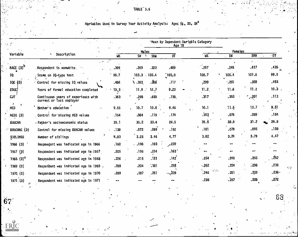
TABLE-3.6

'Variables Used in Survey Year Activity Analysis: Ages 18, 20, 24a

Variable Description

'Mean by Dependent.Variable CategoryAge 18

FemalesMales

WK SW 1 SNW OT WK SW SNW 07

- RACE (Dib

$

IQ

EDUC

CJT

/

MED

MEM (D)

DUNCAN

DUUCANC (0)

SIBLINGS

1966 (D)

1967 (0)

1968. (D)c

1969 (0)

1970. (0)

1971_(D)-I

,Respondent is nonwhite,

Score on IQ-type test

i Control for missing IQ values\,04.

Years of formal education completed

Continuous years of experience withcurrent or last employer

.

' Mother's eduCation

Control formissing MED values

. Father's socioeconomic status

Control for missing DUNCAN values

Number of siblings

Respondent was indicated age in 1966

Respondent was indicated age in 967.

Respondent was indicated age in 1968

Respondent was indicated age in 1969 .

Respondent was indicated age in 1970

Respondent was indicated age in 1971,

'

,399

98.7

.486

10 3.

.363

9.55

.154

25.1

.138

4.03

.160

.205

.226

.200

.209

....

,

.269

103,3 .

\ .303

11.9 .'

.298

10.7

.084

35.2

.072

3.25

.198

.196

.215

.204

.187

....

.323-

163.4

.168

11.7

.650

10.8

.119

33.4

.089

3.44

.193

.214.

.151

:181

.261

--

'

.489

'101.0

.717

.2 -93.739,

9.46

.174

24.5

.152

4.77

"239

.163'

.142'

.228

-.-:,,,28

--

e

.297

100.7

.299

11.2

.317

10.1

.103

28.5

.101

3.82

--

.254

-.262

.:::

k

.245

106.4.

'.251

11.6

.351

, 11.6

.076

38.9

.079

3.24

....

--

.248

.224

.261

:267

.417

101.6

.358

11.2

' .201

10.7

.089

31.2

.095

3.79

--

...

.265

.298

.209

.228

.435.2,

99.5

493

10.3

.113

,9.51

.184

4 24.8

.150

4.47

4. .4

.252

.238

.238-

.272

67 68.

.4

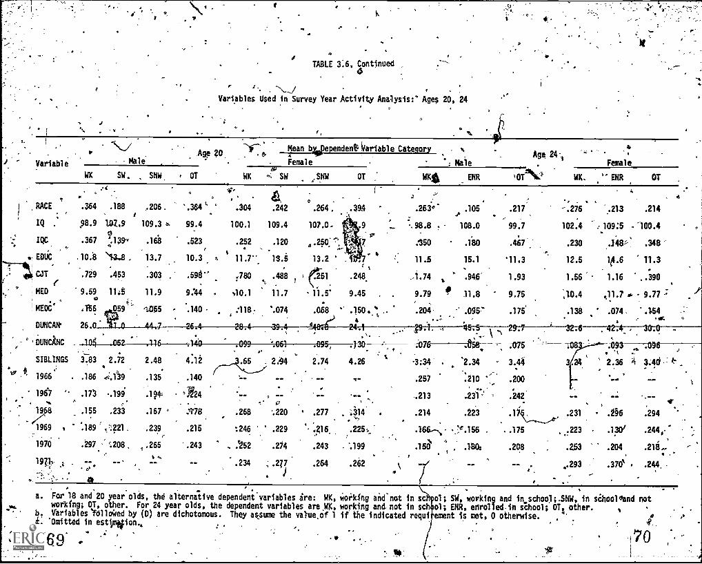
is

TABLE 3.6, Continued

Variables Used in Survey Year Activity Analysis:* Ages 20, 24

-\JAge 20.

Mean byAge

Variable Category N

1

. 6

Variable Male Female Male

WKee,

SW. SNW, OT WK SW SNW OT W1411 ENR

Age 24.1

,OT2Sij

Female

WK. " ENR OT ,

4 1 S

0 V° V aI 0RACE x.364 .188 .206. '.364 L ' .304 .242 .264 , ..394 .263°.

i .IQ .' p8.9 102,9 109.3 z, 99.4 100.1 109.4 107.0.. .9 ... x.98.8.

oIQC .367 .139 .168 .523 .252 .120 .250:".-', :350.. I.

. EDUC .10.8 NUJ, 13.7 10.3 ,.. 11.7" 13.5 13.2 ' - 11.5

CJT .729 .453 .303 .594" .780 .488 : (i.C51 .248. .1.74e ... 1 .i.

MED 9.59 11:5 11.9 9:44 110.1 11.7 - 11.5' 9.45 , 9.79, - 10

MEOC ,116 059 '',..055 .140 :118: %074 .05 8 ' .150. % .204. .!.

DUNCAN' 26....

° 'DUNCIINCfP, s.

SIBLINGS 3.83 2.72 2.48 4.12 (___,...,k65 . 2A4 2.74 4.26-_---v

-3:34 .As, it

. .

' 1966 . .186 ..f39 .135 .140 ..- .257

1967," .173 .199. .l p, 424 -- , -- -- , .213

-. 0.

. ; .r . 4

.105 .217 -.276

108.0 99.7 102.4 ...

.180 .467.. .230

15.1 '11.3 12.5

.946 1.93 1.56

11.8 9.75 ;10.4

'' .095:" .175 ..138

. .075 -:

'2.34 - 3.44: . 3.24

.210 `',.. .200. ..

an - .242, .

8 .155 .233 .167 '' .118 , .268 %,220 * .277 . Ii14. .

.214 .223 .1i.ka, .231,1969 . .189 1 ,:221. .239 .215 :246 .229 l 4216.. :225,, .166.-ti .7,4%156 . ..175/ , ..223

1970 ;297 " :208, _.265 .243 .. :252 .214 .243 . '.199 .150 . .}80 .208 , .253..19Th ;.

.... .234 ,: .217 .264 .262 \ .... .... ,.293e)1

.213 .214

109:5 100.4

.348% .348

1e.6 11.3

1.16 ..390

.11.7 9.77.

.074, .154.. o.

..

.093 :096"k

2.36 3.40. 4" .A .

.... --

rt.

.296 .294

.1.30/ .244,-.

.204 .216-,,370`. .244.

a. For

,

18 and 20 year olds, the alternative dependent variables ire: WK, Working and.

not in sc ol ; SW, working and in.school;.SNW, in sihoolland not

. .. .

_ working; OT, other. For 24 year olds, the dependent variables are .14K, working and- not in soh ol; ENR, enrolled-in school; OTz other. ,b. Variables Yellowed by (0) are dichotomous. They assume the value,of 1 if the indicated requi ement is met, 0 otherwise. ,

f. 'Omitted in esttmilion., :,

4r.

f i 9 7.n .

.

110'

Table 3.7Os

Variables Used in Survey Week Activity Aitalyiis: Ages-18, 2p, 24a-%

t.

0

Variable *, Description MalesEmp UNEMP

RACE (01b

IQ '.4.

.Re4ondeni is nonwhite

, ,

Score on IQ -type test

'.3141.

101.1' .-

.399

.101,1-

IQC.44'

EDUC

C4T -

MED

MEDC 6D1

liCANDUNCANC (D)

SIBLINGS

.Control for missing IQ values-t.Years.of formal education completed .

.

Continuous years of experience with.current or last employer

Mother's education

-Contrbl for missing MED values

Father's socioeconomic status

Control for missing DUNCAN values

.Number of siblings

%

..

.370

11.4

.544

10.1

.112

30.2.

.088

3.63

.194

,

4

,

.417

11.3

.052i

10.4

4.135

30.6,

,..108,

..,

3.511

11966 (or Respondent was indicated age in 1965

Mead by Dependent Variable Category.'Age 18,

OLF

.270

.

,

105:4

.332.

11.8

.079

11.2 .1

.082

38.4

.091

3.10

.177

1967 (i) _.Respondent was Indicated age in.1967N.,.

-.198 .191

1968 (D)c Respondent was indicated age in 1968*

.414 .355

1969.(0) 40" Respondent.was indicated age in 1969 .197 .208 t

1970 10) , Respondent was indicated age'in 1970 .191 ,

.4

1971 (0) Respondent was indicated age in 1971- -

71

a . 4

. 2

.37D

.209

. 217'

FemalesUNEMP OLF

.,257, .050 .113

102.8' 100.9 102.9 .

.267, .327 .369

11.4 11.0

.532 .oso .113

10.7 10.3 ,, 10.6

.088 .10

31.7 29.5 , 32.8.4

:089 .115 :104

.3.68

a.

.4.00 3.67

.257 ,.223 .258

',256 .234 .255

' :226 .253 :257 3.

'.26i :290 . '.230

4'

8

Table 3.7, Continued

Variahle

Male d\, EM? WIMP Ng

RACE .297 .395

IQ 100.5 102.1

IQC .i9444°(771)4'7277--,.. ...,

EDUC 11.8 12.2

. , UT :747 .034

.140 10.2 11.0.

IIEDC .131 .134-.

SONCAN 30.8 32.2

- .

9

- DUHCANC, .090.1

.134.-

SIBLINGS. 3:45 3.60 -

.10

1966 .- ".. .170 : .101--

1967 .190 .151

tsa -.192.

.143

1969 .201 _210

1970' -,47 a .395

. 1.971 --

Mean by Dependent Variable,Category.

.Age 20

Females 'Males, _Females

. OLF UNEMP o OLF EMP UNEMP OLE% EMiP 1IUNEMP 'OLF

, I fc.

.191 . .281 .401, .318' .219 ,.500' .236 :254 .392 .224. Oil

--...._ .

109.2 102.3 99.0 102.3 100.5- . 98,7 -1.06.29 103.3 99.3 101.1 ,

.185 .208 .313 .315 - 14 .319 .500 7361 .

r

:229 .354 .305

13.7 : 12.1 11.9 :11.8 .12.1 '. . 11.2 13.8.- 12.8 1 11.9 11-4-'

.120 .957 .076 . 184' , 1,71 .150, )B33 1.82 %'.174 .271.. .6..

11.6 10.5 10.3 10.2 lo.r . . 10.1 11.2 10.5 0:41 k 9.91

.948 .098 .156 .120...

.191 .300 ,..- .083 .125 .i01 064

43:4'4'r 30.8 28.9 Ai

%

. tor30.9 32.4 24.0 37.1 34.2 28.2 3O.5

. .101.083 .094 .164 'f'.

. .071 , .075 .083 .083 .063. 0398

.

2.66 . 3.39 4.02 3,68 3.15 4.08 2:60 3.13 3.68. ; 3.30,

c.

- .-. . . .

.148 -- ,,, .245 .150 .264.

,..

...,

--

.194 ... . .224 4150 ..167- d.. .

. N 4

J.

.. . -

:219 .261 .239 .287 .214 -- .145 .208.

.291 s' g60

.228 .245 : .240 .224 .181 .200 .209. .212 .228 .4.239

.211 .251. .203 .'.247 .156. .325 - .153 :2.C7 .190 .220

... .243 ;318 .242 .... .287 .291 .272

Age 24'- 7

,

, T'

0

,)...

'

.7 a. Tbe alternative dependent variables are:. EMP, employed; PHEMP, unemployed;. OLF, but of the labor force. . .

b. Variables followed. by (0) are dichotomous. They assume the value Of.1 if the indiCated requirement is met, 0 otherwise.

,O. Omitted in estOmation., ,* ., - ...-...

73I

,

TABLE 3.8

Constant

DETERAINAHTS Of SURVEY YEAR ACTIVITY: HALES AGES 18, 20, and 243

0.4a,

Age 18P44..e

Variable in /;t2Lfilill..t rob K 1

4Ena.ln)i . {Prot, Carlrob OW la FRY-NR) y2 (d.f.) la 41-1R311

RACE

.

.221 .503 .235 7:59 (3)

i'.161}

.664

(1.61) (2.73) (.85) - (3.05)

IQ: . .006 .014 .014 5.90 (3) .019(1.22) .(2.31) (1.11) (2.91)

b 7

IQ; :424 .343 .564 9.85 (3) -.005(2.97) (1.84) (1.73) . (6.03)4 a

EDUC .872 .616 -.210 302.98'(g) 1.609, -

(16.41) (8:73) (3.27) (7.74)".

CJT -.103 .131 .191' 35.55 (3): 2.214(2,05) (2.43) (2.69) (3.17)

KED ' -.027 .039 .108 12.35 (3) .010

(1.17) (1.27) (2.14).

(.30)_

..,MED0 . ... -.246 tk:021 -.315 3.09 (3) -.451

(1.41) (.09) (.94) (1.63)

tOCAK .013 010 .004 16.78 (3) . ' .009

(4.06) (2.50) (.60) (2.28)

DUNCAKC -.479 -.285 ' -.025 '7.51 (3) .369-

(2.69) . (1.17) (.07) (1.25)

1.35 (3). ..

sOidu :

% .011 .018 .047

4/ (.48) k (.59) (1.09) . (417)

"4 , Li,. -:... ; 41.

.(1.76) (2.18) (2,i6) ..,

9.21 (3)-:-

(1,44)1966 .12 ' .536 -.373

-- . ..

1967 ..-- .009 .445 :369 . - 5.62 (3) -.255

1969 -.105 .142 . :65? . 4.76 43) -.262(.63) (.59)' (1.67) (1.10)

1970 -.450 .

(1.21)

535.

I,

19.35'19.35 (3 .....-). 1.879(2.55) (1.34) (3.81)

o-9.603 -10.276 -3:574 ,, 2)0.01 (3) -22.414(13.71) (10.63) (2,40) (18.45)

.

2711 s

.

Age 20

ro M1RST1 Ildrro1544Pgil 1.2 (d.f.),.

.987 14.13(3).(3.22)

0..

.029 .011 .12.6413)13.25) (1.091

..0

.205 .457 3.27.(3)

(.70) (1.61)4

1.505 -.079 325.33 (3)

(13.38) (1.33)

-.375 -.073 14.34 (3)

(3.10) (.80)

. .045 .019 1.17 (3)

(1.01) (-44i.aw.,)

..-.391 - 375 3.81 (3)

, (.97) C (1.18)'

.015 ' .002 9.07 (3)

(2.93) . ' (.24)

1.127 -.258 s 10.70 (3)

(3.15) (.81)

2.52 (3)-.026 .020

(.49) (.50) .

(.25) .(1.24)

3.57 (3)-.096 -.458

1.69 (3).002 . .090

(.27)t

.114 '4.001 2.514(3)

(.34) (.00)

-.339 -.349 16.30.(3)

(1.05) (1.08)

,

-24.501.

6

4,571 365.33 (3)

(1506) s (2.16).J

.r

1816.

X2 (df) 744.30.(42) 1382.83 (42)UA

J

,,

4

76

..

TABLE 3.8, Continued

a

Age 24

(d.f.),In fProb (E106) . eri443.1

Variable LL_612" -.246 -.450

(.95) (1.71)

IQ ' .026 -.003(3.49) (.28)

IQC .144 .676(.69) ' (2.78)

VAC.003

(11.96) (.06)

CJT

. 473,

-.204 .049(3.74) (1.10).

MED. .022 .003(.67) -(.08)

.,

.HEX-.222051 3

...

i04 (.82)

DUNCAN .0133 .003. 84). 60.( i '

3.56 (2)

12:69 (2)

.7.83 (2)

*144.74)

16.04(2)'t'

.45 (2),

.

0. " .69 (2)

.95 (2)

.20 (2)

.27 (2)

.02 (2)

.1.16 (2)

1.23 (2)'

3.45 (2)

a.

OLDICANC .109.

-.104

SIBLINGS

(.011 (.46).018

, '''

1966 -.013 -.039

196. 4 . -.034 .318, WO (1.05)

1969_ -.139' .301(.52) ' (.92).

1970

(1.84)

.587.-44)

Constant -10.90 -2.56(12.29), (2.41) `

,N'.x2-(df)

Ratio Index

.

152.29 (2)

1484485.59 t28T

.215 ,

valuel in parentheses. IN

ft,

78

1

TABLE 3.9

DERIVATIVES EVALUATED AT TEE MEAN: SURVEY YEAR AtaveLTV, MALES, AGES 18, 20, 24

VARIABLE

AGE 18

Prob(WIC.) Prob(SW) Prob(SNW)

RACE ri042 .003 .039

./Q -.001: 0. .001 :

IQG .-.065 .059 .001

EDUC -.125 .147 -.004

CJT .009 -.037 .024

MED .002 -.011 .007..,

MEDC .033 -.050 .020

DUNCAN -.002 \.002 0.

DUNCANC, -.068 -.083 .009

SIBLINGS.

- 002 0.1

.001

1966 -.057 .011 .033

. ,

01967 -.014, -.042 :050

1969 .007 -.045 .024

..

1970 :047 .-.134 .072

a.

?

4.AGE 20 'AGE 24

Prob(OT), Prob(WK) Prob(SW) Prob(SNW) Prob(011 Prob(WO Prob(ENR) Prob(OT)

.0.

0.

.005.

-.017°,

.005

.002

-.003.

6.

-.142

-.005

-.024

-.323'

.053

-.004.

.104

-.00Z

,

.121

.003

-.013'

.304

-.036

.001'

-.078

.002

.047

.001

,010

'.060

-.018

.002

-.01.3

.001'

-.026

.627

-.041

.001

'.001

-.013

0. .

.052

-.oqg

-,.=..059'

-.044

'.014

-.002.

.014

-..001

-.019

.002

.008

- .049

-.020

.002

.003

0.

.011

.001

-.001

-.006

-.016

.006

-.033

0.

.051

:.004

.006

0.

-.017

0.

-.009 ,

'.001

1.003

._025

.025

.044

.006 -.113 r .050

.008

-.066

.:.04

-.056

-.167

-.059 .004

.001

-.020

.010

.064

-.003

-.002 /

-.002

Acit

-.019

-.009

-.050

.O01

.0134...

..006

.014

.015

.

-.006

.084

.039'

.040

.173

-.002: -

- .003

.004

.012

'-.003

41

. Table 3.30

Determinants of Survey Year Activity: Females Ages 18, 20, 24a

A

Age 18Age 20

Variable.11{Prob (Sit)} WC {Fret41%.} fPrif413zil} ihro }:}4) intr5 1434},1n reP11667M) iu ro x2 (4.f.)

IQ

IQC

DC

liEDC

DUNCAN

40U1CANC

SdLIKGS

...

1969

1970

1971

...

.633

(4.13)

.026(5.19)

.076

(.53)

0.225

(3.43)

.106

(1.50)

,132(5.18)

-.175--- (.87)

.012(4.24)

-.139

(.70)

-.023

(.93)

--090(.55)

.039

('.41)

.117(.73)

',

.

.8 : :

(5.27)

.035

(1.34)

.184

(1.13)

-.064(1.01)

-.297

(2.51)

.099

(3.45)

-.417

(1.81)

.008

(2.35)

-.180. (.80)

-.017(.62)

-.040

(.22)

-.387

(2.01)

-.242

(1.27)

.130

'(.73).

-.003

(.37)

.201

(1.09)

-.363(6.09)

..-.978

(4.51)

-.010'(.318)

.311

(1.45)

-.001

(.22)

.215

(.96)

.009

(.31)

-.391(1.86)

-.279(1.32)

-.062

(.30).

34.64

31.26

1.0

69.91

.32.36

34.56

. 8:90

-21.45

2.9f

11.47

3.62

6'.45

3.59

(3)

(3)

(3)

(3)

(3)

(3)

(3)

(3)

(3)

(3)

(3)

(3)

(3)

.."-,

4

'

(3.76:!

.026 .

(3,61)

-.101(.45)

1.130(.00)

-.168' (1.95)

.032

(.93)

.305

(1.05)

.002

(m)

-.324(1.06)

.011

(.30)

-.028.* ( -.12)

,268

(1.18)

.439(1-.95)

.634(2.34)

.016

(1.73)

,727(2.94)

.140

(11.80)

-.803(4.61)

.001

--.179

(1.96)

.283

(.84)

-.058(1.25)

-.469-(1.62)

46-.305 .

(1.09)

419-

.(.07)-

-- 53( .15)

-.m(2.10)

g

.64)(1.64)

-.271

(5.57)

-.841

(7.67)

-.017'(.63)

-.072071

-.005

(1.26)-

.183(.89)

-.002(.09)

-.569

(3.10)

-.758(4.09)

-.348(L97),

.

17.89 (3)

20.32 (3)

13.3b (3)

371:36 (3)

'76.44 (3)

.1.57(4

1.99 (3)

6.30 (3)

3.59 (3)

"2.15 0)

11.73 (3)

2.17 (3)

9.45.(3)_

tonstant ,

lz (4f)N

Ratio Index

.7.287

-($.021

* -2.022(2.23)

3.571

(3.87)

107.66

447.41. 2055

.082

(3)

(39)

26.280

(18.89)=

20.938

(12.65)

4.331

(5.42)

440.75 (3)

1207.12-(391946..-.265

.1 4

-

TABLE 3.10, Coitinued

Age 24

Variable,. In fiaLifel(11 JT

fhWK) e.(d.E.)in

RACE .385 -.806 26.51 (2)

(1.23) (f.80)

IQ .012 -.008 4.53 (2)

(1.32) (1.46)

IQC .095 .287 , 3.27 (2)

(.31) (1.81)

DOC .394 -.192 81.52 (2)

(6.24) (5.57)

CJT -.110 -.631 103.88 (2)

(1.57) (10.17)

KED -.003 -.028 1.18 (2)

(.07) (1.08)

KEDC -.312 -.178 1.34 (2)

(.76) (.96)

DURCAN .002 .001 .12 (2)

(r29) (.24)

DUNCANC .417 .097 1.21 (2)

(1.07) (.44)

SIBLING -.075 -.027 2.45 (2)

(1.31) (1.01.)

1969 -.993 -.475 13.07 (2)

. (2.81) (2.66)

1970 -.693 -.620 14.88 (2)

(2.21) (3.48)

1971 -.274'. -*.670 15:29 (2)

(.99) (3.90)

Constant -8.090 . 4.080 103.41 (2) - ,s

(7.01) (6.40)i2- 0f) 436.58 (26)

N -- 1487

Ratio Index .167

a. The absolute value'of asymptotic t-statistics appearinparentheses.,

81 1

r.

.0

It.0

:TABLE 3:1T

DERIVATIVES EVALUATED A.14$134EAN: SURVEY-YEAR ACTIVITY, FEMALES, AGES ;1$, 20/24

-

a

1I4

VARIABLE

AGE 1s.

Prob(WK) Prob(SW) Prob(SNW)

:.

.

RAPE -.144 .078 .096',

i(ii , -.904 .005 0.

IQC - -.031 ' "-.002. .019

II/EDUC -.007 ,.067

*

-.016.

. '

CJT . ..050 .078 -.031

MED -J:022 ,023 .007..

,

-... -v061,MEDC ', ' .037 ' --.024

DUMCAN -.002 .00r .001 .....

a

AGE 20 4 * AGE 24

Prott(0T) Prob(WK) Prob(61) Prob(SNW) 'Prob(OT) Pr (iK) Prob(ENP) Prob(07). 4

..

-.030

*-.001

.014

-.044_.

r.097

-.008

.047

r.00l

.,

,-

'

4

.

....0.39

.

0.

4451.

-.101

.138-

0.

-.002 '

o:

-1636

,

.002

-.013

.121

, .002

.002

.023

: o.

-

_,

'.025

.001

.028

: .054

,

r.026

. 0.

-.008

0...

-.047

-.002

- .036 .

-.0710,

16..--.114

9.003

-.013

-.00.

.151

.001

. ct:060,

..027

.130

, .006.

.045.ol. '

'

.

- .027

.001-

0%

.019

. .004"

40..

-.011

0.

-.178

-.002

/p.,060

:.647 .

-.134

-006..-

-.034

0. 'I0*. .'DUNCANC r .020 -.027 -.024

,--A4........, .. ._. l'.

f ....'. cjo

' ALINGAI :i(' 10", -.004-'9,°,)'

1/41 . ,..12.6i . .0V0 -.303 008

1M, .035 .043 -.056

, _ 4...-1. ft ...

.,-.

I'.043

,

-.0431971 ' , .006

.031

.0q?

..-.

-.036.

0

-.021.

. .

..-.053.

.

,

-.014

.001

4/.087 ,.str . *

.090

- .

.. ..019...o.

- -.026,*. .

.001

:007!

,030

1,03,6

_,_'

.011

-.002

-.015

.(108'

..a02

.

.029.te 1

'0,

,

-.079.*.

.

r .

-.031

.008",

.123.

.616

-.003

-.035-

-.021

'.!

./015

-.005 ,

-.088

-.124

-.4.40

4

o.

14

4'1

4,4

OUNCANC -

SIBLINGS

1966

Table 3.12

Detetninants of Survey Week Activity: Males lies 18,;20, 248

Age 18 Age 20 .

EtP

.0

ln ro

ftro,44gri, ro x2- (d.f.)

121 roPrris244

(d:f.) 1 --

(2,36) f4

Ca! .'

14.041 (2.42)

-.016 -.015

-.118(.99)

0 -.052(.29)

-.148 -.161 --.

1.062 -

(3.48) (2.81) ,_

.. -.344(8.24) (1.27)' .

-.069 -.032(3,40) (-1.03)

.286 .247z

(1.70) (1.06)'

-.009 .--.007

(3.92) (1.90)

-.160 - -.072(.97) (-30)

c

10.83 (2)

.

16.71 (2)

1:00 (2)

,

.

13.03 (2)

094.19 (2)

.

t 11.95 (2). .

2.92 (2)

- ' e

.48, (2)

,

.96 (2),.

.

--.013 4-:024-";-----r-i--.1.9512r.(.63)- (:78)

8..91 (2),

72.80 (2)

-.184 .224 . 4.45. (2)

by .(1.25) ' It (.97)

.... -.226 .330 7.39 (2.) *

(1.11) (1.39) -,7:..".,..- , 4

:...,

. . .

5.361

1 (8.58)

'

75.51 (2)

% 2712360.22 (28)

.076

.

(1.77)

-.358

.(.80)6.31,

(1.15)

10.29-:018- -.010(3.18)

-

-.391

(1.28)3.47

-:537 , -.439 v.

102.96

0 0.15).. I' .

0.85y,

ima -1.103. 79.50 (2)

(7.78) '_ .-(2.20)4. , - .

(2)

12)

.-- .005 .101 , 6.51(2).(.18) " (2.18) s'

-'

- Is

. - .-

.62t.'

(2.15t:

-.008(2.48)

-.298(1.17) .

:603(1.54

. -.010'01.89)

.25)1.70)

:--

..

".

.

41 .68

,,-

7.08

3.90

-1.07

.80

.

6.62

(2)

(2) . '

(2).

(2)

(2)

(2),

(?)

(2)

...t,

.

-3)111-

(.26)

-.200

(.85)C,

.081 e.(.31)141.

.044(.21) .

et

.248

(1.19)t

.035(:70)9

(.68).

re, -.049. .( .13)

.313. 1.86)

s .8660, '(2.57)f-

--10.152(12.36)

41. t

''. 4:615.(3.79)

.,

,

1

10.23

1818$10.46

.?1)

.. .,(28)

,v

x... . .19A ..

1 . .. . 4

41,

AN,

s.

a

9

, TABLE 3.12,,Continued

Variable

Age'24

InMAAR" , -4 (d.fs)151WYPT:

RACE

IQ

IQC.

mix

OJT

,

( :,,, ((.638

.0ii -.02525. -

.19) - (11?5)

-.620(2.10) r (.92)

-

6.10741

.208(2.29).

.815 -.506

(4.77) (1.27)

.- s,

4

. s

a

mimic

SIBLINGS

1966

1967

1969

1970

Constant

N "

7.

DUNCAN

a. -.048

(.93) _

.663(1.46)

.008- (1,28), .

-.123

(.26)1 ,, .0:

(.86) 0.20.050 .105

-- -.384 -.594

(L.03) (.89)

.323 _ .045

(.79) (.09)4

-.244' .054.

'OM. , .N48)

6 .

.059

(.14) (1.51) *. .

7.672 3.879(5.70) (1.85)

.046

(.53)

4 .953'(1.98)

-,007(.62)

-.535(.68)

'a'

x2 (df)Ratio Index.

4-21 (2)

4.81 (2)'

4.42 (2)

9.63 (2)

35.39 (2)

2.49 (2)

- 2.70 (2)

11:69 (2)

.48 (2)

1.58 (2)

4.24 (2)

---.79--(2Y

:64 (2)

3..34 (2)

. 1.

36.38 (2),

1484156.45 (28)

.166

a. The absolUte value of asymptotic t-stapstics appearin parentheses..

S

*el

a

I '1110;.

. t

, 1ABLE 3.13 * .

.,.

DERIVATIVES EVALUATED AT THE MEAN: SURVET,WEEKACTIVITY,41ALBS; AGES 18. 24_24,

aI.

,

VARIABLE

ACE 18r

AGE, 20

Prob(EMP) Prob(UNDU9 Prob(QLP) Prob(EMP) Prob(UNEMP)

IQC

EDUC

(RACE 7..072 .030

.IQ - 003 0.

v.022 .003

447.004

CJT -.090'.247

,

'AM_ .002

'MC : .046 .002

DUNCAN -.002 0.

DUNCANC, . -.030 .004

%

SIBLINGS

1966

*.004 -.003

-.075' .042

r-:-- ? 196Z -.045 .020

1969 -.053 - 028

,AGE 24

Prob(OLF3 Prob(EMP)

. sois -.pp ,014.

(' .033 -.011

\

.003. -.002 0.

..019 -.030 -403

.026 v -,053, .001.

.

-.157 ..165* 6.060

-.002 --:".003

r,049.

-1. .001

: ,.001 -.001 0.

. .026_ _

-.042 .015

-.002.

-.002 .001

.034 ' 7.017 -.002

.02-6 .008 -.001

... w024 -.003 .008!

/ .-.002 .001,I

.

!(033 -.012

.052 -.003

-.103 !. _:023

.004o

.007

0. , ,

.001

-.007 -.016 .

Prob( NT)

.001

.012;

..003

rob (012)

-1°-----: oor7 ---..ace ----lx-'

IR r.060, .011 k .002

.001 'O. 0.

.027 0. n' -.002

%.00:: I. ..

.001 0.

-.006. "-.001

-.008 .008 -.001

-.005 4-.006 .002 '-

1970

ft

1970 .068At

. S

.

:029-** 4 -'4077 .' :018

.

. *

r`l . .-.020 -.004. .005'

- ----:,

-.013,.

0.

t Ai

. .002

-.001

.007

t .005'.

-.001

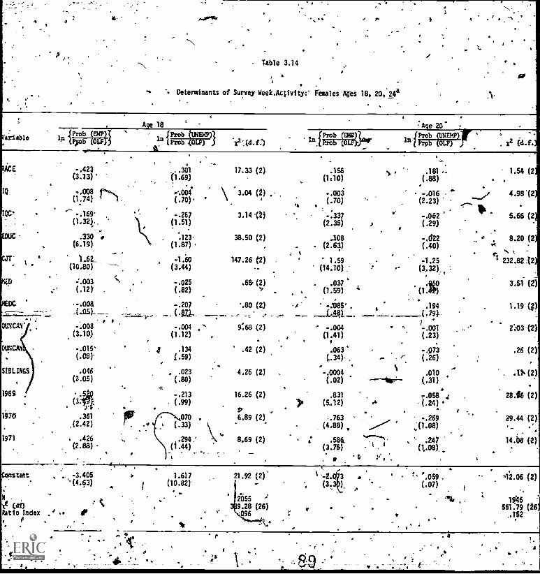
- Table 3.14

. .

". Determinants of Survey Weei,Activity:' Females As 18, 20.'24a

Age 18 Ace 20'Prols(_IEMP

U1Protoriur)tscp rg$10654Firqsariab1e la OT (Preb x2 (d.f:)

f laiPT°1cf1134P xt (d.f.

-.423 .361...

17.33 (2)-(3.13)* 0.69)

.156 N , .181 ,,(1:10) .

1.54 (2

IQ .004-.00874) r4-, (.70," 1

4\ 3.04 0,) ,.

m

-.00i(.70) .(2;13; 7 ,.....7(

4.9812

, .

- . 1110e-

' 5.66 (2.169' , -.267(1.51)

3.1412, -.337 -.062(1.321 (.. (2.35) r (.29)

--..,-

.330 .123 38.50 (2) .108 -.022,

-..._

162 -1.60 147.26 (2) 1.59 -1.25

-, 1

(6.191 (1.87) . . (2.63) (.40)

(10.80)

S(3.44)

.6&-.025 .6,..' (.12) . (.82)

cm -.207 '.80

tmaw I -.008 -.004 ,'". 9:68(3.10) (1.12) .

WNCAN -.015' 4 .134 .42(.08) /.59)

SIBLINGS .046 . .023 4.26(.05) (.80)

1969 .5 -.213(3. . (.99)

..

1970 .361 070,(2.42) (.33)

1971 . .426

dm,294' 8,69

16.26

tt6.89

onstant.'.(4.p)

xe La),

Ratio index,

(2.88) )_ , ,_ ..., -

-3.405

r

-

., (14.10) ... (3,32)

(2) .037.

(1.' . . . (1.59) L X

21.92

20559.28096

(2)

(2)

(2)

(2)

(2)

(2)

(2)

(2).

(26)

'-2. W3 w

(3.

-:685. .a .194

-COL_ (.79)-1 S.. -.001

(1.401)4

(.23)4 I

.063 -.f03G.34) ,- e (.26)

-.0004 .010(.02) ------411-- (.31)

-.058 :) (5.12) (.24)

.763 -.269(4.88) , .....-4 .(i.os)

'586, .. .247.

(3.75) ' (1.08),. .

' ".059(.07)

.

23823.:5021:(2221

1.19.(g)

2.:03 (2)

.26 (2)

. .1 (2)tk

2816 (2)

29.44 (2)

14.1)8 (2)

*12.06 (2)

19'6551:79 (26

.152

a

4

,

TABLE, 3:14, Continued C .

. . . .

IQ

,,"

4QC

Variable

RACE

EDUG

CJT

KW:- '

In 1P1.°1112---"P.( Prob It

.526

(3.06)

001(.20)

.169'

(1.0),

.211 I ..

(6.10)

1.080 .

(12.5Q)

.034.

(1.29).

t

'NEDC

. DUNCAN

DUNCANC

SIBLINGS

1969

Age 24-

niProb (UNEMP.)}.

Ptig)OLF)

(2.68)

-.008(.76)

.

.3E6,106)

;`-,

.1.11

(1.72) itSt

, 61:3

(.140)

-007

. s

-.012 -.681(.d6),

. (1.63) Ill

( . 1001 0.0....

(.22) "" (.03)

-.035 -.475( .16) 41 (.95)

Q .03711 .64) . (.73)

.468 -.310(2.44) (.88)

IVO .523 , -.491(2.79) , '- ,,(1.35)

1971, ..480 W -.201(2.69) ' I (.62).

ti

x2 .(d.E.J.

N

.72 (i)°

1.75 (2)." -

13.30 (2) '

37.35 12)

172.54 (2)

1:69%(2)

2.73 (2) ,

'

.06 (2)it (

.91 (2),

2.82 (2)-.

8,04 (2)

11.74 (2)

8.86 (2)

0

Conitani

i2 (a)

NRatio Index

. °A,

-4.238(6.62)'

- 2.574.

(2.13) -rfr 44.26 (2)

527.01 (26)1487.208

;5

J

a., The absolute value of ttymptotic trstatistics appear fn parenthes0s.

0

9 0 .

. .

AIL

oft

f

Aca

-

A.TABLE 3:15

ti

DERIVATIVES EVALUATED AT THE MEAN:' SURVEY WEEVACTIVITY, FEMALES, AGES 18, 20, 24

. .

.

VARIABLi

AGE 18 AGE 20. AGE 24

I

Prob(Emp) Prob(UNEMP)

I

Prob(OLP) Prob(84F) Prob(UNEK8) Prob(OLF) Prob(EMP) PrOb(UNEMP) Prob(OLF)

a

c.,

sr

RACE 1

IQ

'1(11:5P

EDUC

.,6iTT

MED

,IIIIC

y DUNCAR

DUNCANC

SIBLINGS

,

1969

1970' ..

1971.s

'-,:.

-.117

-.002

-.031

".076

.467:'

0.

.007

-,002

-.009

.010-

6157

.092.092

.093

.

.044

. 0.

-.016

-.003..

-.205

-.002,

-.017

O.

.

.012

0.

.

- .021

.007.

..,

.074

.002

.046

-.073

-.262

902

.0 11

..002

-.003

-.010

-.097

-.071

-.100

'

-At

c

4

i

9

-'.032.

0.

-.074

.027

.417

.007

-.026

:.001

.017

n0.

.201

191

"%1.33

I

...004 -

4.001

.007

-.004

-.105

"e'001,

.012

O. I

-,005

0.

-.027

-.045 '

-.006

1-

-.036

.001

'.072

T.022

-.312

-.009

.015,

:001

-.012

0.

-.173

-.156,

-.127.

......

.105

0.

.033

.046

.252

.008

.009

0.

0., '

, , .

.010

.111

.126

/:112

.

1

.012

0.

.Q05

-.001

-.031

0.

,-.017

.0.

-.011, .

0.

. -.016

. -,021

-.013

.

.

.:.116

0.

..-.038

-.045 ,

:-.122

-.007

.638

V.: '

.011

-.010

-.095

-.105

,-.098

a

e,

1

oe'

9 2:

IndependentVariables

.

IQ

I9C

MED

NEDC.

DUNCAN

,

puromc

518111165

ENROLLED .

.

CONSTANTRZ

SEE11

TABLE 3.16

Regression Estimatesof Educational Attainmente

34

1

. ,

.Age 20 44: '4

i

Parsonsc ' Lazeard Grilichese

,

Kohen and Roderickf

Males Females Combined AtteMales

-Black . WhiteMales- Females

BlackFemales

..

.149(1.03)

- .638

(7.99) :

-2.01i(15.80)

.257

(11.96)

, -.936(6.52)

,

.018

(6.51)

-,261

(1.25)

..

-.105(4.64)

T :558

(9-20

.746

Is.e2)

.,--

.037

(8187):

-1.959

(16.83)

.202

(10.601

-.790(5.40)

.014

(5.79)

-.128 ./'

(On)

-.114

(5.38)

1.294

46.48)

. .454

44.

-.070)67(.91).

.036

' (11.56)

-2:011

(23-.25)

.228

(15.81)

.-.871(8.47)

1 .016 l

(8.67)

-.186' (1.37)

/ -.104

(6.96)

1.531(12.11)

-;

.1804'(.85)

.005

(1.78)

--

-.212

(7A31

--

,

-.721

(3.84)

--

.056(13.33)

.150, (6.76)

. ....

,

.

t -.164g

(5.32)

,

f

-.43

(2.3)

.049

(8.2) .

i

. .116-(7.0)

n.a.

--

....

-!01 ..

(3.3),0.

.

' --

.051

(11.02)

"--

,

'..-t.

.33

(9.10

d.

....,

'

'...

-.07:(2.39)

.031

(4.17)

.18

(2:96)

..

'

-.08(1.99)

1

.038(7.83),

.32(10.08)

.. ...

A

'

-.02( .81)

, --

4

.021-

(2,9)'

. .

VA

,15t. (248)

--

-.06(r.s6)

--

6.076".505 A

2.062: 1504

,6:712..435 --

1.8501480

6.537:470

'1.9662984

8,432:27

41.a.

l06,

.

.

6.505.311

1.63-, 863 /

/'

n.a.

-.365

1.61362

4.20:30n.a.

707

7.97.21

161

5:16.31

n.a.

645

9.50117n.a.162

. 1 d

.-- t statist4cs in parentheses.' *. ,

,.i

b. The sample is respondents age 24 at any survey 'eat., inc uding those enrolled in schoOl. '

1c. Parsons :1974)3 Table 3, line 4. ,The sample is nonenrol ed male youth in 1966. Other variable included in regression. father's education.lazear (1976), Table 1, column (c). The sample is nonenrolled male yalth in 1969. 0they variables included in regression. family income,urban residence at age 14i'resPondent living,with parents at age 14. . '

e. driliches (1976). Table ±t, line 3. The sample is nonenrolled male youthiri 1969. Other variables included in regression: culture index,father's occupatiod when respondent was 14, regional location at age 14, age, and,nonresponse control for father's occupation.

f. Kobel, and Roderick (1970, Table.A2. The sample is respondents age. 8 to 25 in,1968 (males) or 1969 (females) who are employed-full timeas wage and salary workers. Other-variable dncluded in regression: index ot high school quality. ,..

. Lazear's,yarfable is ectually.numbeP ofOramily !ethers.' .

.a. Not aviffabje.

.

I. :73 . .,,

f." .

cso

APPERDIX'III.1

Logit Analysis

Tim,components of the,model--status (equation 2.1) and, turnover (equation

,2.3) -- analyze the fact:it's associated with An individual's choice of labor m rket

activities from among several alternatives. The genei-al choice problem ca

easily bb expressed in standardutility maximization terms. The utility of the

jth alternative to the ith"individual iss

U = U (Zij. j lj

where,

Zi= vector of characteristics of indiVidual

Xj.= vector of characteristics of alternative j,

(A3.1)

0 = vector of parameters,',

.eir vector of random elements.

The choice of.alternative'k from'aming the set.of possibilities implies that st.

01k 2,Uij for all i. . (A3.2)

Since we neverhave'information on all the relevant characteristics of either

yndiViduals or alternatives, we cannot perfectly predict the choice made by each

individual. Instead, we determine-the probability that an individual with a>given

set of characteristics will select a particular alternative. Then the problem

is to estimate the vector of parameters, a, that is consistent with the assumption

that.the chosen alternative most frequently maximizes the average persbn's utility.

0. , .

Since the dependen't variables are qualitative, indicating wheth r an activity,..., Pr

is chosen, and are therefore ;discontinuous, the usual least 'squares assumption of.,.

. ..

a homoscedastic error term is violated. That is, the error term varies systemati-

cally with the explanatory variables., resulting in. inefficient estiiilatton of

94.,

1 72

S

. \regression coefficienti. Moreover,' estimated probabilities based on least squares

regression may well fall outside the zero, one range. The solution to this pro-.

blem df limited.deperident variables is to employ maximum likelihood estimation,

*where the. likelihood function incorporates theimit,restrtction. In a choice

problem involyng two alternatives the most common procedures are probit (tasgd

on the rioi-mal -prObabifity distribution) and logit (based. on the logistic

tiution).. Choice problems involving more than two alternatives, as-in our status

and turnover models, can only be' estimated,practically usinj multinomial logit

procedures (see Melson, 1976). A more 'detailed description of the multinomial

)logit model than will be. presented here can 'be found in tierlove and Press (1973).

.. ,,

. , .'For the sale of convenience, consider\a choice problem involving four

. .

mutually exclusive and exhaustive pqsiibilities. Suppressing the error term,

the probability that the ith individual selects the'''jth alternati-ve 'is given by:. ,

,s

E31X

e -, , ('A3.3)

Pik 4 :,X4- ;E es . .

m=).

1 .

Xr= vector of independent variables associated with the ith01.

ehoice. .

.s-..

Since one of the four ,alternatiVes Must be selected; only three. of the fOur'sets

of coefficients tam are uniquely defined.- Wet' normalize y setting-the -faun)) set',

- ... . ., ..._.

of coefficients ,e..9ual to zerb.(B4 =`0), :. .

* .-- * ;

, .* ,19 a- . . %. C

,

. 4

. . bsilt-this normalizatioividual coeffiCients .can easily be interpretftd.Li . ,.

q o te, t h'a Vi dropping tithe substcri pis ,

....., ,, - ".?:.

7

i ',4. * , .**. -4w'

.,- , ...

JtO

4

10 4,4

1,1

6.

lneta X

lh(esiX) = 13:XP4

e

(A3.4)

Thtis 046 is the percentage change in the odds of selecting alternative J relative toF

A

selecting alternative 4, for a one unit change in Xk.. The earginal

effect of Xk.on pj, the probability of selecting alternative j, is given by

.., .

aPi .''

----"-- Pj(ilk Pli3lk Pe2k P,31330 .(A3.5)

aXk

. Expression (A3.5) holds as well for alternative 4, when $4k

= O. Since the proberD.

bilities given by (A3.3) musttby definition sum 'to one, the partial derivatives.-

given by (A3.5) must, sum to zero over the four alternatives.

In interpreting the logit estimates it isimliortant to remember the interdepen-

dence among choices. Our formulation enters all independeft Variables into the,

probability expression for every choice. This allows each independent variable

to directly affeCt the relative odds of selecting any of the four choices.' However,

even if a particular coefficientjs estimated to be zero, the probability of that

outcome is still affected indirectly by the independent variables's impact on

the other probabilities.

Maximum likelihoodestimates of the logit model are derived using the Newton-

Raphson 'iterative procedure, as implemented by Bard (1967). Both parameters ejk

and derivatives evaluated at the mean are reported for eactreselmation. 'Several'

Measures .S statistical significance are available. Each parameter has an asymptotic

,t ratio Associatedwith lt. Asymptotic x2 statistics test the null hypothesis

that all paraMeters estimated for a given, independent variable are zero; an addi-

V.:tonal x2 statistic tests the null hypothesis that all parameters -in the estimation

(except the constants) are zero. We al so port the natural logarithm of the

likelihood function when the probleN has converged., and the likelihood ratio'

.index, an analog to the multiple .correlation coefficient, developed by Domeneich

. .

.1!.

and McFadden(1975Y,. 96

CHAPTER IV

Wage Determination: The. Impact of Personal Characterqtics,Aggregate Economic, onditlons,and Market Structure

In this chapter we examine the determinants of interpersonal 1;ariation in.

,

wage rates by estimating cross-sectional wage regressioris for alternative age groups.,

In 'the context of our overall model, wage idetermination is the pivotal component.

.

--wagirate is a key indicator of labor market success, and deficiencies in the. .

wage determination process are hypothesized to be an important determinant of.

74

dynamic behavior.

The cross-sectional wage (or earnings) regression is an exceptionally

versatile and useful construct. It has been pressed into service to analyze

such issues as the economic returns to human capital acquisition .(Hanoch, 1967;

Mincer, 3974; and Griliches, 1976), te nature and magnitude of\sex and/or\\

race discrimination (Oaxaca,f1973; Blinder,: 1973; Welch, 1973; and kohen,and'.

.Roderick, 1975), the effect on!wages of structural factors such as industrial

concentration and unionization ,(Weiss, 1966; and Wachtel and Betsey, 1973), and

-the-implicit prices workers pay for training' opportunities' and/or working condi-.

*.:tions (Antos and Rosen, 1975;. Thaler and Rosen, 1976; and Brown, 1977). It has

also'been used toy generate predictions of expected or market wages fdr use in

,

other types of analysis(KalackeklandRainds,1970; Hall, 1973; and Mellow, 1977).

.

Our use of the cross-sectional,Wageregression-is comprehensive. In this chapter

4

ti

,

,

we take a. detailed look At estimatpd parameters, comparing ourlindings to those -

.

.

of other,researchers. We then use these estimates to construct Predictions1 . ,

V

, , * .

1'for a worker's market and currienX wIge; these predictions betoMe inputs into sub-. ,

sequent parts of our analysis,../

4

. *

e

4.1 The-Wage Determination Process-

s

. .

A central statement of the comixtitive theory of labor markets is that, giyen

the overall level of real wages, an individual worker's wage is- determined by his

productive capabilities- -that is, by`his innate abilities and investments in

human capital. We designate the wage.that a worker could beexpected to receive,

igiven his capabilities,_ihe-"potential wage," and any premium or discount from'

the potential wage the. "market 'differential." 'We eestimate a model of the wage

determination process that sectorstcurrent wage into potential market differ- .

eptial components. Our specification of the model is taken from Kalachek and

Raines (1976), and similar to the many cross- sectional wage regressions esti-

mated others._

The potential wage is the rental price of those characteristics embedded in.

the Worker. Following the human capital literature, those characteristics are

-identified as ability, education,currek job experience, training,,age,ilealth

status, plus race and sex. The market differential is the systematically explain-.

able deviations from the potential wage. Market differential variables are 41'

geographic location, occupation and industry. These variables attempt to capture

premiums and discounts from the human capital or potential .wage resulting from

.

disequilibrium in the worker's labor market and from his luck or ability in secur-

w ing emplowent in an enclave. Supressing the age variable;'the'human

capital and structural variables are 043uped together in the followingI

model of wage detetImination:

f

where,

a

' a

74

at

= X18 + X72Y c . (4.1)ao

W.= natural logarithm of current wage,

X1=, matrix of ftuman capital variables,

X2=-Matrix of market siifferenti al variables,

vector of error terms- ,.assumed, independent of X1 and X2.

Estimation of equation (4.1) provides, the basis for identifying a worker's popen-.

tial Wage and market differential. The straightforward approach would be to

obtain OLS estimates of equation (4.1) and use fix, to establishthe potential wage

and iix; t cA2\ito establish4predicted current wage.. However, diredt estimation

of the equaiiOn will riot yield consistent estimates bf the true-coefficients of the .

human capital 'variables because of the corre lation between. human capital and market

differential variables. Since more human capital not only results in higher pro-

ductivity in any specific job,.but,alsO routes workers into higher payfing,jobs,

direct estimation of (4.1) will necessarily -produce downward biased human capital

doeffici,ents:' To-illustrate the problem more fully, assume that some portion,

,the-,

. .

XiB, of thevariation in the observe/ d measures of the market differential,}2, is'..

.

attributable to the operation of human capital variables but that there is a com-.

f ;--../pbnent, 4, uniquely attributable to, market differentials themselves (a .component

7

by definition independent of,X1), than

. X2 =X1B. +X7,

Substituting (4.2) into- (4,1) yields.

,where

(4.3

(4.4

'77:

....

,

(4.----"'"4--% { C,

,,

As (4.4) indicates; the total effect of human.capitall,,onsists of a direct, 0, and

".B-

. .'.,v

. \\4trati- - .

directy.

l effect. Because X2.is -not obsevabl-4-- e on. , an in 14.3)

,

can not be. - .

v - eitivated direcpy. Hoi.rever, unbiased estimates of the parameters can be obtained

...

i, . ..

.

by, a two stageprogess. In the first stage, W is regressed on XI, to obtain con-

,*%

7 sistent ,and.efficient estimates of 0* (by virtue of the independence. a X1 and X2)..

In the second stage, W is regressed on X1 and X2 to' obtain consistent and efficient

estimates of and y.

c

,-' the (log of the) worker's pOtential wage is then X fi:.', the predicted

i

value from the human capital (Stage I) regression. The predicted value from..

.

-,

,.. .

the current wage (Stage II) regression is X'0-1- X y. The Worker's systematic1 2

market differential is defined as:

MD El: X2;) - Xjir (4.5)

,

Because both regressions are log-linear, MD summarizes the deviation of predicted..

.. 6

current from potential wage in relative or percentage terms.%,,

,

A more general specification of the market differential is W

the residual from the Stage I wage regression (RESID). Assuming that on average -.

market differentials are zero, points on the Stage I regression line can be idehti-

fied with the potential wage. That ts, for a particular worker's endowment of

characteristics, the regression gives the estimates of current market prices for

elements ln the human capital vector. We can thus take the residual as an estimate

of the worker's market differential, because it measures the (percentage) deviation

between his actual wage and1

the wage we would predict for him, given his endowment

of productive characteristics, from market relationships.

RESID is a more comprehensive measure of the worker's market differ-

ential, it is nevertheless a Melange of cOmpondbts. Ib addition to the systematic

.1 -* 100

70

market differential, RESID include§ the effects of market errors in the wage deter--.

minationpAocess at.thb worker level, measurement error in the wage variable, worker,,st

specific difference's in search efficiency, compensating varistions for training

opportunities' and working conditions, and, to the extent thi the human capital'

vector is underspecified, a potential wage component.2

Of course, even with MD we isolate,some.effects which are really equilibrating

phenomena. A few examples come quickly to mind. Regional wage differentials may. ,

reflect cast of liying differences that, at least foN.w4rkers, may be equalizfng

differences. The i ustry effects may capture unmeasured human capital variation,.

given the crudenes of the years of schooling and experience measures.' The same

might be true of he occupation effects. Again these Are equalizing differences,

not disequilibrium phenomena. The industry and occupation effects might also be

crude proxies for working conditions such as pollution and a whole related set of

job-consumption attributes. The regional effects might reflect degree of urbanization

and journey to wok: In sum, we probably claim too much by arguing that MD reflects

Arely disequilibrium effects: it contains both disequilibrium and equilibrium

effects. As a result, our measure. of the market differential overestimates actual

noncompensating wage differential45. The implications of this overestimate for our

analysis are examined'in subsequent chapter's.

101

I

4.2 Empirical Findings

79

At each age, the wge determination model Is estimated for the sample of all

wage and salary workers reporting a wage of twenty-five Cents an hour or more.

All of the variables used in the basic specification of the'model, alopg with their

mean values ,at ages 18 and 24, are presented in Table 4.1. The potential

,(Stage I) and current (Stage II) wage regressions Pesults-for the age 18, 20 and

24 year old samples are reported in Tables 4.2 through 4.4 respectively. RegresA

Sion results are reported for the combined NLS sample and for separate sex and

race subsamples. The outcomes of several exper ents-with variable, model, and

sample specification are repoi-ted when approPrite. ,Since itie dependent variable\ ,

in the wage model is the natural logarithmof current wage, the,estimated coeffi-Q

cients ate interpreted as the percentage impact of changes in the independent

variables on wages.

Many of our findings closely parallel those.of other. researchers.1 in such._.

instances we do not discuss our results in great detail. In particular, since

countless other studies examine the topics in considerable detail, we do not.

extensively analyze the economic returns to schooling or calculate detailed. .

4.4

measures of "net" sex and race discrimination. It is not the case that are,'

uninteresting or unimportant topics. Rather, it is,simplY.Ochat 6everal eiCel-t

,

ent studies on likese topics alread,y.exist which use NLS youth data. Regarding

1 0

00

"- f'

the economic returns to education, for instance, the recent work of Griliches-.

(1976i 1977) provides a comprehensive discussion of many of e-ecanarnetrilp

problems and presents various estimates. Likewise- udiesby Flanagan (194)\,,

hen and Roderick (1975), and McKay (1975) represent a much more detailed and \,,

sys

ton i

related udies, using other data sovrces, also exist. 3.

. t. ,

Classified by major area, our principle findingS can be summarized

matic evaluation of the magnitude and source of race and/or sex discrimina-*

the-wage determination process than we will attempt. A multitude of

as follows:

4.2a The 1Mpact of Personal Characteristics

1. The potential (StageI) wage regressions reveal that human capitaTdif-

ferences are an important explanation"

for interpersonal variation in wage 'rates.

Moreover, the results indicate that as the aging process continues and the human

capital vector acquires more variability, its ability to "explain" wage differences

increases proportionally. ,At age 18, for example, the R2

for the potential wage

regressionis only .17, but by age 24 it increases to .32.

1

2. Consistent with the findings of everyone else, we find that education

has a large, significant and positive impacton wages. The impact increases

. 4

slightly with age and is greater for, females and nonwhites..

3. Since the wage regressions we estimate arestratified by age and control

for years of education (EDUC), including a measure of potential experience (PEX)

would result in a yinear dependency:

PEX GAGE - EDUC - 6,

103I

(4.6)

4

where AGE is a constant in each regression. PEX contains several elements:

"PEX a CJT + OE + ,U + OLF,

where CJT is current job weribnce; OE is other experience; U is unemploy d

time and OLF is out-of-the-labor force ti .

4'

At early ages, of course, CJT approximately equals PEX, but as worker 0;

tJT and PEX diverge. For males the gap consists forlthe most, part of othe. , 1

(non-current) job experience: PEX - CJT approximates OE. For females,- a 1 r ergr .

portion (which grows with age) of the divergence can be attributed to none hboi, out-

' ,:

of-the-labor force time: PEX - CJT approximates OLF more and more as feMal lae.

With the sample stratified,by age and controlling for education, the Coeff deb%

of CJT indicates the value/

of recent job experience relative to other nonsohiool'

- activities. One would expect, therefore), that the coefficient for qpi. wO,114 be

largest for older females in our *sample. This is exactly what we find.5, t

age 24, for example, tht CJT coefficient is aOligtify,significant .048 in. t4, !

female regression compared to an insignificant .004 in the 'males regressiop

1.1

(Note,.00-in Table 4;1 the mean value of CJT' is approximately equal for male and

females at age 24).

4. Ability (as measured by the IQ variable),6 "self-confidence" (as

measured by ATT the score on the Rotter.test of Internal-Exteimai control) and-

health status (HFP)7 typically have the anticipated impact on wages. Howe

coefficients are frequently insignificant and .the change in wages implied

large variations in-the independent variables is rather modeSt.

; 5. .'Saki ng a vocational program in .high school (VOC) or a-formal train no ,

program (TRAIN) has a (positive impact on wages: The effect of a training p ti gram

is greatestfor'black females,.where it intreasesges by 10 percent at a 18

1°4

and 17 percent at age.20. At age 18, a training program has no significant

.82

impact on the wages of, the other sex-race groups; by age 24 it has a significant

impact for all except black males. Taking a vocationil program in high school

initially benefits white females the most, increasing wages by 8 perc4nt at age 18.

At age 24, the vocational training program variable has a significant coefficient

in only the white males regression, where a 9 percent increase in wages is indi-

cated.8

We experimented with specification 'of the-training variable without great

success. 'Replacing TRAIN. with DTRAIN, duration of training in months' (adjusted

for intensity), the estimated coefficient is positive, but less significant

than t4aft---of TRAIN. (At age 24, for instance, DTRAIN has a coefficient of .907

with a t-value of 3.26 for the full sample.)

6. Married workers receive a wage premium that declines sharply with age.

Disaggregating by sex reveals that married males receive a large premium that

declines only modestly with age while females begin with a small premium that

turinto a discount and becomes successively more negative after age 19.

7.- The potential wage.pegressions include a control variable indicatingti

that a respondent-i; currently enrolled inSchool. Its coefficient is negative

ant highly significant, indicating a wage discount of roughly 17 percent at age 18

and 10 percent at age 24. If we do not include the enrolled variable, the

coefficients of the training variable increase and those of the IQ variable

.decrease,dramatically; they are turned into proxies for enrollment statuS.9

If

equations are estimated septrately for the rionenrolled,.the results are not

seriously altered.

105r.

4

0

-;

83

.

,The impact of school enrollment on the wage rates of male youth has also been

examined by Parsons (1974) and Lazear (1977). Both studies use NLS data and

#'obtain results that are comparable to ours. Lazear attributei,the lower earn-

.

ings of enrolled youth to equalizing differences--u'studenti optimally choose

more fldible and easier jobs at the cost of loWer wage %" (p. 170.

4.2b The Impact of Aggregate Economic Conditions

Figures 4.1a through 4.1d 'chart the estimated coeffidents_of the market

opportunity variables. Recall that the 1968 variable is omitted in estiMation

consequently, the estimated coefficients of the'other.variables indicate how real

-->.

wages vary by year, relative to 1968, for the age and skill level`e

of the respondent." ,A secular upward tren in labor productivity would argue for

rising real wages over time- -that is, negative coefficients on, the year variables,,

before 1968 ,and positivecoeffidenti after 1968.

The findings are quite interesting. For males, real wages--standardized by

age and skill,level,-increased dradatically during the boom period of the late

1960's. When aggregate labor market aanditions deterioriated in 4970, however,

real wages stagnated for older workers (aged 22-26).and actually declined for

younger war

Several rdsearchers, including Freeman (1973), and Smith and Welch (1976),

. have documented and commented on the dramatic improvement in the economic posi-

tion of.hlacks during the last half of'the 1960's. As Figure 4.1b i ndicates, we

also find that during this period real wages of black mal6s increased dramati-, .

.cally.. Moreoverebecouse we control for variation in-human capital, .this increase

0,

is net of any improvements in the acquisition of human6apital of blacks.' .

106

tip

. . , .

relative to white's that occurred during the period. Finally, while Freeman (1973),

is

84

and others find that black incomes are much more cyclically sensitive than whites,,.

.

our results indicate, that this sensitivity does not come fromLa widening of wage_ .

. .

,Tdifferentials during the economic downturns among those'who are employed, at least

t o .\

for the time period and.age group we examine. . ,.

/ ...

For females, we find that real wages increased sharply in 1969, and stagnated. .

in 1970 and 1971. The increase in 1969 is particularly noticeable for black, .4 \

females.. The real wage of an 18-year-old black female increased by

18percent between 1968 and'1964; the ,increase at age 24 was 24 percent during the.

same one...year period.

(4.2c The Impact of Market Structure

4

1.. Controlling for measurable ham capital, race, Sex, enrollment status,

and the state of aggregate economic conditions, the structural variables have a -

'massive imPaceon wages. When they are added to the set of .independent variables5 2

the R is increased by about .20 at each age. By age 24, the current (Stage II)

wage regression accounts for fully one-half of the' fnterpersonal variation in wage

rates.

.

2: The magnitudes of specific occupational, industrial and location,al premiums..-

.. . ,

A or ditcounts are.substantial. For workers the data identify as otherwise identi-i

cal, wages vary by ulibto 20 percent depending on locationWidifferences and up to

50 percent for occupational and locational differences. Workers living in SMSAs

receive wage premiums of roughly 10 percent, with no systematic. difference for

'being in acentral-city as opposed to elsewhere within a SMSA. Major discounts are'

assocAated with working in the South, particularly for black males. Professional

and managerial 'workers receive the largest premium; service workers, the largest

discount. Transportation and communications is the industry group. with the

1 07 *

!largest premium; agriculttre, the largest disCount.'

)

*If , eft.

1

3.: The estimated impact of the huMaii capital var)ablei on wages ,declines-

. _. .... ..

. . . ...

. ..-..

*.20,t6 40 percent for males and 4o to 60 percentifor females when we include , -.

i .... ---7,/q ., *-

structural-variables the regression. This detline:suggests 'that e4pcation and :',

reining play important indirect roles. in routing worker's alirlg-occu-.

patiqqs an'd industries:* We,also find that; controlling for cation afia indus-

try, the magnitude of estimated sex and race discount d ines;ikarply.12 In

. . .

(ther words, blacks b,d femalesi?e denied equal acces to,h0er,paying jobs:. ,

, 4.3 Further Evidence

4.3a Union Membership and Wage Rates

The NB did not obtain inforda ion on* ion membership until 1969. (1970.".

for females)-. Consequently, we are unar to in lude any union membership- variables.

.

i n the a9e, stratified regressions. What we can do; however, is estimate the wage

model,for wage and salary'workers employed in 1970, addirig4ears of age (AGE) to!

the,human capital vector and union membeesTOOtttinguishedby'three dichotomous,

variables indicating mbership in an industrial(INDO), craft (CRFU), orAgover4'

medti white-collar, or misceljaneous (OVO) union) to the vector of market Of-f

. ferenetia) variables.. . ft .

... 'Regress.* results With'the sample stratified by are reported in Table 4.5',

.

Th4 estimated union premium is subitantial, particularlyif the worker, is a niber0 ,

,J,...).

. .

of a' craft union.where the premium FS. about 30 percent.. We 6 not-find a. signifi-.

..,

4

mrt difference in the magnitude of tge.predurby sex, although the proportion ofri, ;

leMales'yTho are unionlentersds much smaller. .A

.0.t

k a ,

3b *yage Determination for Yo!ths-andsAdults... A Comparison

Wecaricompare.the.results from the combined, ages sample With ,results from'

, theage stratified sarnplee As expected, in the combined ages:regressions, the

age variable has a si4ea6le positive.cotaicient. Controlling for schooling,

,<

9,

-11

i

. e

Co

- 86.,

I

age futiO'ae,proxy f1nc ns as or enottial experienCe. Foibmales, a year of potential,

. ,. eiperterici *at a s

edxcatI fs 'dec s

fi rrtifng 'in a a

Smallv.impact than a year` of education. For'female, .

re important to wage; than potential experience, con:-

context our earlier finding that potential seriously over-.

'stOes h tualelweri Ce-fdr females. The other coefficients 9n both stages /of,

the regrestions are exceptionally robust under the earlier,specfication.. .

Kalhchek and Raines (1976). use the mature-mOes data for 1969 to estimate

essentially the same wage. determination model. Our results- with the youth data

are remarkably stmilar,to-theirs,. thd,major difference being that eve 06 not find

a lower return to schooling for blacks. (They included aTace-education inter-

.

.,ten variable, and its estimated coeffici.ent was -.019 with a t-value of 4.35.

If we include, such a variable (not shown) its coefficient is .004 with a t-value

R\ .,

of .6). A minor difference in-rtsults that our estimates of occupational.

ands, industrial- premiums are somewhat smaller, while. union membership premiums.., _

* . are lightly higher.

4.3c Race, Sex, and Wage Growth

In Figu$* 4:.2, we have stratified the sample of wage and salary workers\,

employed in 1970 by age, race and sex, calculated the mean hourly wage for each

grOup, and charted the results.

In.contrast to our earlier discussion, which examined how wages at,a given

age vary over time, here we look at hOw wages at a given 'time vary with age. The'

figure indiCates very cl6arly a source of major concern: only white males make

major /progress during the age 18-28 period. In fact, the average hodrly 4-6;70,

increases by .only about fifty cents between ages 18 and 28 for the other three,

./. 0

-

.40

groups. Results from the wage regressions indicate several possible factors. con-

tributing'tp the extremely flat(age-wage growth curves for blacks and females. '4

109

re, .

87

blaeks have.less schooling than whites. The effect of this is two4, 'I

fold. More whites than blacks are enrolled while working (see Table 4.1). Sjnce46 ,

we find that being enrolled in sciool is associated with a lower wage during the

years.of heavy en9plIment (ages 18-22) wages areirshed down more than.propor-itionally for'whites. However, by their middle twenties, whites emerge, with signifi-

cantly more education (the average white male, for'instanceE,h.a.i' a-,1 .9 year.advan

tage over.the average black'male at age 24). Given our finding that a year of

education-increases wages by more than a year of general experfenCe, the sTope of

.ethe wage curve is increased at older ages.

,

Second, ther0s.a growing divergence between actual and potential experierice,

for females (as implicitly, documented by the increasing significance with age of

the current7job-tenure variable in the female-age stratified, regressions and the

poor performance (relative to males) of the age variable in the females-all ages

egresIsion), Th$4 suggests that. less "investment" in market work by women may be

dn important factor contributing to the widening of the male-female wage gap with

- age.-

Finally, the regression results indicate that.specific occupations and

,

industries pay various discounts or preVums, and tqatiplacks and females Are

systematically denied equal access to those.mith large premiums. Very few blacks

or females become managers and almost no females become craftsmen or work in

.construction, all activities that pay substantial premtums.' The occupational-,

industrial distribution at ages 18 and 24, reported in ,fable 4:1;_revediS

_dramatic improvement in the occupational position of white males compared to that

of the other groups. -Of course, some of the improvement--thetgreat increase in

the percentage who are professifial workers, for instance--results from those,

0

a

f, i * o .4 1'

(4

- ,

enrolled at ager.)8 completing theie educatiOn and moviOnto the labor market.

88

Conclusions

We have estimated a straightforward specification of the'standard cross-

sectional wage model. .In generdl: our results confirm what is already well known.

Investments in human capital are productive, significantly increasing one's wage..

Controlling for measured differences in:productive capabilities, blacks and women

receive, substantial wage discounts, but.during the late 1960's, blacks effectively

narrowed the differential. We also'find that, net of measured variations "in worker

>, .

quality, specific occupations and industries' pay premiums or discounts. Although

'I

/i

human capftal is important in.roUting indivrdluals into.high,paying sectors, blaoks

,,4 1: ,

and women Are, nevertheless, systematically denied equal access and this is.

. ..,

responi.fble foe a.large part of race and'seX3.differentia1s. finally, we find a/ _ .

surprising ,decline'in,real-Wdges among workers employed during the.recesgionary

, - . . , .

period ofthe early 1970's....*** "- ''' .

.

In this chapter we' have eimpi Weicali. dentified the Market diffei-ential in a

4,-

static setting. However; its existence at any, one time implies nothing' substantive- .

about the competitiveness of the labdi. market. Simply knowing that some workers,,,

receive wages inconsistent with their capabilities does not necessarilyinvalidate

,.

the competitive model. The labor market is not a-bourse where adjustment are, 4

1

ge

instantaneoui. A' ore aPprdpriate lest is whether market differentials persist

:;.

.

over time Whether they.stimulate equilibrating behavior which results in -'-

their liquiddtionp or resist.eroSion' because of segmentation or 'ba lkanization .

of the youth labor market. Subequent'Chaoters provide such tests.

.1

(Rosen (197 ), for

-Footnotes to Chapter IV

example, contends that workers implicitly purchase

learnilhgopportaittes thrOugh wage reductions. ;'The difference between

the market rental of a worker's existing ,Skill.arld V.,,s actual wage is the

shadow*br implicit price.he payg forlea4ing" (p. 328). For younTworkers,-

.

. .

it is 'especially likely that wages are tieing foregone to obtain training

°opportunities. The magnitude of the error caused by this emission is- - .

reduced,iiihen we'use the instrumental'Variable approach 0 define the market',

_differential.t

I

2Receni research examining the residual variation in earnings suggests. .

.. i

that the proportion-of unexplained variance attributable to underspecification_ro ,

'

diebf'the human capital vector maybe quite large.- Lillard (1977), -for examyfe,

i

using NBE4R-TH data estimates a variance cdmponent earnings model that sectors

the residual variation ,in earnings into' permanent and 'transitory components

4

and finds that unspecified worker spetific factors account for 57 percent of, .

residual variance. (Lillares huthan-capiial earnings regression exp)aiqs,

30 percent of the variation in annual earnings.).

extensive review 'of one topit; see the recent surveys by3For4 an

Kohen (1975) , Kahne(1975), and Marshall (:74).

1/4tudies using data from earlier time periods typically -find higher -

returns to schooling for whites (Hanbch, 1961, and Weiss, 1970). More recent

evidence., however, suggests that this is no longer true (Weiss and Williamson;4

1972, andWelch, 1973), that therelas'been a sharp convergence in black and

white returns to'schooling, acticularly.for younger workers&

4

112

S.

.

. - 5,For audetailed examination of the impact that discontinuities-ins e

labor market experience have on female earnings, see Mincer and Polachek.41

(1974).

6In the NLS the IQ variable is constructed from scores on .various

alternative tests as recorded in the respondents' high school' records.'"

,The .test results thus refer to a period that in most cases precedes`the

completion of formal schooling.. Unfortunately, 'however, IQ scores ,a)1:4

- missing for.many respondents (the exact missing value rates are.given

in Table 4.1). Moreovei., the non-availability rate is sysiematicaIl

related to race and sex.- Indealng with the nonresponse problem, we-

assign mean values and denote the responderrt.with i dichotomous variable.

.

In extensive experimentation, Griliches (1976) found that thiS selectivity

problem did not seriously bias the results for-young men. Also Griliches .

and others who estimate wage regresions with the-NLS data frequently use

scores from A "knowledge of the world of work" (KNW) test administered ,

z , . .

withirrsthe NLS as an alternative ability; measure. We did not use the

KNW variable because the test on which it .1. based.is not the same fdr,

,f-

: males and females. (For.an analysis of Vielideterminants and implicatiOns,

. .

for _labor market sucOess of scores on the occupational information test

(KNW), see Parnes'andKohen (1975)); .r

/ConstructtOn.of the ATT and HFP varfables was complicated by the

timing of the relevant survey questions.: The .Rotten test which was used

to construct ATT was first administered -to the males in 1968 and the, .

females in 1970. Consequently, for males -thy indicated age "in 1q66 or

1967 and females 'the indicated age in 19b3 Jr 149, ATT scoreswere,

, ..

h. .1

determined by their responses in 1968, sane 4970 respectively. To. the.. .f

. s .

'extentthere is attrition in the two samples,

.

the dummyvariable indicating

"4'4V

113

.

. .alionresponse to the Rotter questions becomes a proxy for being the

indicated age in 1966 or 1967'for malex and 1968 or 1969 for females.

'Additionally, there is a potential prOblem of reverse causation in that

responses to the Rotter questions may be influenced, by previous economic

status. See, Andrisani and NesteT (]974) for an eended analysis of the:

later problem. The problem with HFP is that health status was not

ascertained every survey year. In constructing HFP, we implicitly assume

that health status did not change- during years in which no questidns were

asked.

8In estimating the impact that,vocational and training programs have.

on wages, what wemay'.in fact be observing is a select?bn effect:_ Those/

who reckive-training. may be significantly More able than those who do not.

9The NLS obtained training information only if the respondent was notA ,

enrolled. Also recall the 'estimated inffuence IQ .has. on educational'

attainment in Chapter III.

loUnfortunately, the timing, of the male and female surveys was not

coincident. For a given calendar/year, males were interviewed 'during the

/

final quarter, females during the initial quarter. .Thus, fdr instance, in

the 1968'survey year females were interviewed a full 9 months before males%

Since wages were deflated by price level figures far the relevant quarter,

,hOWever, the impact of this disctepancy should be small. If real wages

are increasing over time, the effect will be to overestimate4slightly.theI °

extent of sexual discr ination.

11-In addition to capturing cycliCal effects, With ag'e hef4:constant

the year dummies also capture any "vintage" effects:

'414

ti

: 4

12The decanetn the race coefficient still is present if we omit the

localidhal variables. In noting the decline in the race coefficient, recall

that We inCitide A.RACE=SOUTH interaction term (RSOUTH) ,the Stage II4 .

'specific tinn.:. If4,RACE entered as a single variable'in Stage II, its

coeftici t would be:

O.+ a

(RACE) (RESOUTH)

'where

SOUTH i s th mean.of SOUTH..

"Whis conclusion--that it is a concentration of blacks and females in

1

t

o

log paying jobs and not uhequal pay for equal work that is relponsible for

, large portions of the net male-female or white -black wage di4erentia1=-is

-/r

in agreement with that of other researchers. See, for example, Oaxaca

(1973) and 1311nder (1973) .

14The determinants of male-fethajesAffprentialsein unio

are examined in the appendix to this chapter.

ership

15Ior similar evidence with the NLS sample restricted to youth who did

not go on tocollege, see Parnes and KoheW (1976).

IN

1.`

,

°

S

,' TABLE 4.1t

Variables Used in Wage Regression

t

a

a

.

'r

,. Age 18 Age 24. .

Terilfle Description Miles ferules Hales -. Fouler\ 1.10 tes nonwhites iih"ner-ornOftes a %CMOs Konatites Ltites ...-sratite.

. ' a .. ( .. IHwy Capital Variables (Sr) .

Oa (0)4 Respondent is nonwhite. 0.0 1. 9.0 L 0.0. 1.SEX (0) Respondent is feral*. 0.0 0.0 1. 1. 0.0 0.0

10 , Score on IQ-type test 104.6 95.3. 104.1 95.3 101.6 95.1, -a

0.0

4.

105.6

1.

1.

95.5 S.1f1C (0)' Control for missing 111 .

vital.) .27 .53 .21 .43 :24 .38 ...15. .41!r ,

MT Scaling of responses toasp abbreviated versionof the Rotterrieast cfinternal -Este 1

Control. ileascres theextent to which theindividual believes hecan control his destiny.The Tower the score. thegreater'is the belief Ofself-control.

iTTC (0) Coritrol for,4

missingATT values." .

ECCC Years of formal educationcompleted. ",, .

SST (0) Respondent is serried.

TRAIII (0) -Respondent ever enrolled vin a formal trainingprogram. .13 ` .14 .14 .22

s .

. . -22.82 ?3.70 23.22 23.54 21.40vg.:24.0J 22.54 . 23.36. 1

dz- ..21 .22 .09 .12 .21 .22 .12 ti 4

"i11.76 10.95 11.57 11.01 12.59 10.68 s 'tilt p.e6

.oa .09 ' .16' ' . .12 .72 .61 ..69 .55

VOC-(1)) ReSpondenterer enrolledin a muttons-1 prograain high school.

.42 , .4, .48

.14 .17 .22 .19 ..11 .11 ...,

24 .16s

CJT Continuous years ofaS ..excerfenee with current .

r attest toplOytr. .36 .24 .3a .22. '1.67 1.46 -1.69 1.16

1 AP (0) Respondents (vealthstatus is fair or poor. .14. .09 .05 .06

'mu. (0) Respondent enrolled in .fowl education program. .54 .41 g , .49 / .43 .14 Am

AalleilloPortunity Variablesc

104 (0) iespondent was Indicatedage in 1966.

1967 (0) Respondent was indicatedage In 1967.

1."0 Ao)d, ,pe9rogreoswas Indicated'

a(o) Respondent was indicateds i9

age is 1961.

1970 (0) Rtspendent was indicatedage in 1970.

1971 10) lifspondent was indicated194 In 1971.

.14 409 .06 .96

.20 .16 . t .26 .24

.20 .20e

. - .22 .20

-'..20 . .26 .26 . .21 .23 .17 .24 .20

.20 .21 , .23 .29 , .16 '..19 .22' .21- n

.20 .19 .25 .25 .16 .20 ..24 ' .27.

4. .i I

.IS .2$ . .n ..

0

Variable Description

Structori1 Variables (Ze)

Occwatioo:

1201 (0) Professitual and. tedsoical workers.

WIG (0) Moaners and officials

SALES (0)...-

Clerical and saltsClworkers

"..,.,01AFT (0) Craftineo wad tomes

0118 (D) ',., Ceuratim,4.

LABOR (0) Laborers. includingfaro laborers

PRSU (0)d Print.. .M.4001dservice workers andoccupation not reported

IsitrastrY:"f

Aal (0) 1411eultera lad forestry

--ccitSTR (0) Mining and Construction '4

PIC (0) Itworfactertag.

TUNS (0) Transportation andComussicatioe

411

TABtE 4.1 (Can't.)

Variables Used In Wage Regresilon

Roe 18

0

Aye 24

Males recites ..., Males ferulesIthites nonwhites Id lites Amanitas "Iliites nonwhites telig1.3111

\49

\.05

.02

.16

.11

.3,

.24.

.13

.0.12

.28

AS

0

-

. ,

.03

.01

.13

.06

.32

.27X

.18 ,

.05

.08

.33

Al

.

.,

.01

.01

; .57

I .01

=.11

..01

.29

0, An

0.0 ,

.16

1.04

.

%

.05

.01

.45

0.0

.16

.01

.32

0.0

.,13

r05

at

.22

.09

.14

.19

.25

.07,

.05

.02

.11

.35

.08

...

.. .07

.02

.08

.15

.35

.21

.12

.05

- .11

.39

.07-

0

.27

r.45

.01

...,..it

.01

.12

9.°.01

.22

.05

.

.12

- 0.0

.33s--

.0Z.

-.26

0.0

.29

:01

0.0

.27

....03

T1JJX (0) losgle and Paull '-\.

Trade u ' w

nx to) Fisszi lesvraoce.and al Estate

SERY (0) Services ,.

PA (6)d Public Adnialstraticoand Jadeite)* not reported

Et:Katie* of farrientResidence:

CCITT (0) Respondent lives in SMSA(central ,city)

RCM (0) Respondent lives la SatSA(not actual city)

EAST (0) .Etstiro raglan.k0.

LEST (0) liewitris 491cu `o-

.30,

.09

.07

.04

.24

.32:.

.261)

.14

.30

0.0

.31

Al '

.21

.12

.10

.0S'

.50

.15

.13

.07

.63

.83

.1$'

.46

so

'

.36

..24

-"".15

..0

.03

..25

..34

:24

.15

.27

0.0

.24

47

-.21

,

.23

.31

.16

.10'

31

.16

:20

.07

.51

.51

42

.27 .

p.17

.17

.04

*.07

.31-

.35.

.22

.19

.30

0.0

.29

1.00

,

,

'

'.1S

.11

.07

-.154

-.51

.12_,

.14:_-_- -

.06

.65

.65

.15

.87

.

.14

.43

.04

.07

.30

.35

.22

At.30

0.0..29

1.0)

.1T

.38

.15

..05

.52

-.15

.12

.11

.S7

.S7

.20

.

sons (0) Soul/ors -reel ' '- . 0nom (0) Race -south In nom

nee/ale-.

/_____,,-- '

MU (DO iorth-centrel Mica -

Pellendeet Variable (ill .

lila 'lateral logarithm of, t

current wage -t. Varistotts followed by (0) are dicaotoroes, Thy MUM ms va1ii I if tae rosterted mut rimegn Is vet. 0' camas,.6. lksartuondents are assigned the rein value of tae variable for valid resoons and then wesoced bi a dIchatoeous variable.

e. la-estication. Uses* iriables are included with the More coital variables to sue Stout 1 regriSsido.6.. Oaitted la, estioatioe. . C.

. . t:

117"

rt

4-

. ,

e J ,. .3 (5921) (98' ) Or ) Ise. ) (tel) .001) ' (991) NV ) (65' ) (SS' )' (02'2) (EE'Z) )-

(WO (62't) (02' ) (9E' )._(WZ) (09,Z) (g1) (trt) (it' ) (ES' ) (26't) (96Vr

(IS' ) (26' ) (ZZ' ). fLE' ) (05't) 00) 0161

1161 8C0' 220) 510: 800'0 E5k* 660' Zt0' E20' 110' our- 021' 9tt'

-- -- --.

(091) (80) (12'Z) (90'E) (98' 1. (22'0 (tE' ) (96' ) (9E1) (SUZ) (05'1) (E1'2) (6t'1) (00)' (8E't) (WO (Z8' ) (60' ) 920'- tar- 100'0 OLO'r 920' 070' 600'- 820:- 6E0' £10'- VW' AEI; 0E0'0 OCO'- Ot0*- .100:- CEO"- 700'-

1

.

610' 020' 000'- 800'd 080' ,S60' KO' CEO' 210' 810'- 201' ' 511' t

110' 220' 900'- 110' , 250' 870' 69g (trZ) (00) (P51) (Lrl) (W) (561) (tL'Z) (25'2) (Lt't) (E21) (L04E) (90) 150'0 290' 6C0' 600*- 810 - E80*- --,"

, -- 090'-' E90*- t70'- 820*- Ztt'- 611*- 196:

W24, (511) (21'2) 125t) ,(81'1) (0E1) ' 02'0 (95'2) (25'2) (20'1) (09-0 (WO 190*- 990'- 010'- 210'- 690'0 650'- 510' [901- 210*- 150'0 960'0 880'0 WA

..

14:41.'4) ica'01). C.VS) ior'cl (51'0 150') - (9L's) (L6'5) (tS's) (ZL'S) (v1 1) Orr) ;c-s) (14; 0 ,q(4., V) '',,'L) L4 ..-1,, 11;,t. cOW- S4I''' Co :..1. mr. Or- MY- ar1''- new- SW- zo*- sou- for- Top, 01..

_

1,:1*- lir- 261'.- '

7 Wl) (411) (481) (es'i (091) (mi) (0re) WO (ore) WO (08' ) (80't) (E9I) (er ) 00'0 (Cr ) two (is' 900'- LEO'- OW- LEO'- 650'- Mr- 260'- 001', 560'- 211'- 090'- 050'

- Pt0'- 810:- 1Z0*- 110*- 800;- SZ0*- diM

ziPi) (ebl) ter ) (2sl) (0'2) (92'OP (IL' ) (2i') (90' ) (10' ) (68't) (18' ) (85' ) (ze'e) or ) (ss-i) (20'2) (50'E) LOW- 120:- ZOO'- 20:-- ,070*-- ES0*- OLEN 010'- 100'0 900'- 690'- EEO'. 000*- E20*- 700' 540'- 9E0*- 750'- 1i7

. . 86' ) (L0'2) (98' ) (4

..

`2) (90'1) (Ot't) (E01) (56'4 (WO (78'2) (EE' ) (85' ) E0' ) tar ) (sr ) (92' ) (96") (801) St0' 200' 910' St0' 810' Et0' KO' 910' -CIO' 780' 910'- 1E0' 2O0'0 110' .210*- 100' 0E0' 2$' 20A 1.4

86* ) ,,(E07) Air ) eZE1) ( '0 ) (911) (a' ) (601) (0. ) (60) (601) (181) s 10E' ) (WO (98' ) (Let) (60'1) (50' )

Lt0' - 009' 810:L " ',CE00 6E0' ' 920' pr- 200' 5 C00*- E50' 001' ' LOO' 020' 020' al' 070*- COO' ... _. Utra

69'P) (401) 46L'£ .

(591) (LEI) (SZ'E) (60' ) (01' ) ( 0'0) (66' ) (96' ) (1E1) (00 9) (14''9) (WS) (Et'S) (87'E) (WE) a 240' 980' 990^ ' 99)* 111' 621'

,

E10' E00*-- .

-la 5E0'- 550' .C90' 191" 261' 091' 161' 051' SCE' 424

v , . . tea (ern) Ors) Ora (so'S) (Ln) (2E't) (Sri) (SE1) (WS) (69'2) (65'0) (69'9) (69'8) (69'7) (56') (9510 (76:5)

920' - 650'1 .6C0' LSO' SEO' 950' - 6E0' ' PLO 6E0' PLO' 6E0' 190'

. 820' S50' 8E0' 250% 9E0' 550' 2n12

(CZ' ) (80' ) 60 y oe' ) (901) (es'i) ter ) (82' ) (ee' ) 00') (so' ) (9(' ) Me' ) ( '0) ter ) Nil) r ) 091) too'- 100' 'OW- ' 020*- 620' t

050' 520'- 010* EE0*- ZOO' 200' EN .

' -

900' '0 t00 920*- EZO' - 090' XII

(iv ) (t0.1 (og; ) ltt. ) '(2t ...) (o' ) (cri) (99't) (eir ) (89' ) (06. ) (es'o (91' ) (sr ) (oz' ) (tt- ) (09' ) (19' )

100' 100' t "0 '0 200' MO', 700' 200' 200' 000' 100' '0 100'- .,

'0 (00'- 200'- ma-- (ZE' ) (091) 4IL'L) (60'1) 00'0 WO (9s' ) (Cl' ) (eel) (we) (til) (ere) 02'4 (iiri) ter )_ (80' ) (99' ) (eve) 500' 520'- f0C ' 120' 120*- 021'- E10' E00' 250' 890' C50*- 0W- SOn ' 9E0'. 910' 200'- 110' .211'0

(6/7) (WE) (9 C) (90'0) (06' ) (56'2) (10'2) 126'ZI (00'2) (6E £) (80). (861) (Z81) (99'2) '(50'2) (tE'2) (00: ) (00'2).

E

100' 200' ;200' COO' 100' COO' ' ZOO' COO' 200' 000' 200' POO' 100' ,200' 200' 200' '0 MO' -te

(E9'Et) 85'11)

PrbOt) 60'51) (OE'8) (Lt'6)

182*- IC12:- Let'- 6E2'- 012"-

(erz) (et' ) ' (2ri) (eel) (68'1) (8514

550' Coo'- r- 250' -- 800' 020-

. .

let) (Lt) (91) (St) (0t) (Et) (21) (It) (01) (6) (s) to (9) (5) ,(;) (e) (2) (1) 'It it I II I patliq403'

f

alPIN Vela ,

pau4quo3 a414M KDII18 pautg-off , "amm 4,215

latdaeS 103 saiewa

_ sat7H

a6y zsuotssa.thav 06,11 it a0725.Pue I 411/15 '44

2'0 atilt/

1.'

7F3F

S. .

:AA-FT

-MR ,

Cts.,472

1 2 . ; . 0 E

SERV

.- .1t5 - .132 -.122 .011 --

(2.35) (2.83) (3.25) ( .12)

.155 -- .193 -- .182 .172 --

(1.05) (2:76) (2.92) ( .68)

Y -- .089 .116 .104 .139

(2.01) (3.47) (3.90) (2.71)

.066. .121 .104 .163

(1.15) (3.22) (3.35) ( .46)

.086 ' .103 .093 .206

(2.13) (3.12) (3.62) (2:66)

y .

.021 . -- 115 .080 -- -.017.

( .51)1(3.41) (3.05) ( .06)

0.

-.184 .... -.302 -.258 -.356

(2.42) (5.23) (5.59) (2.34)

..1736' .140 .159...

(2.63) (2.99) (4.19)t

_: .188 151 '.171 -.. -.023

(3,49) (3.47) (5.02) ( .23)

.176 .159 .7 .163 -- .119 -.

(2.52) (2.93) (3.80) . (1.17)

-.167 -.121 -.123" -- -.144 -

(3.10) (2.96) (3.771 , (1.99) A-..,

-.043 -.127 -- -.092 .011

( .74) (2.68) ' (2.51) . ( .15)

--A -.037 ....055 -- ' -.041' .-.368

( .63) (1.14), (MO) (4.51) ,

.367 .190 '.118 ... .204 .175,

(4.31) (3.23) moo' (5.11) (5.37)

-..

.353 .321 .. .221 :-.285 .270

(3.02) (3.03) (1.63) (4.78) (5.01)

.217 .195 .136 .197 .

,

176

(8.18) (8:35) (4.28) (9.44) (10.17)

.132 .111 .118 .192 J- .172

( .98) ( .88))

(2.09).(5.89) (6,17)

.

.248 1225 .133 .165 -- .165 --

(5.06) (5.55) (3.79) (7.14) (7.93)

.092 ,059 A- .071 -- .176 .138

( .70) ( .50) (1.84) (6.26j (6.11)

-.253 -.273 -.230 '-.313 -. -.230

(2.10) '(2.97) (3.42). (6.15) (6.91)

-.283 -.244 .137 -.: .119

(1,21) (1.04) .(2.24) 12032) (3.53)

-.053

.

-.003 .154 .. .092 1.119

( .80) / ° ( .05) (3.36) (2.521 .14.20)

.063 .104 .162 .127 .107

( .86) (3.82) (2.85) (2.89) 43.95)

'.

-.165 -.128 -.154 -.129 , -.124

'(4,76)

(2,88) (3.00) (3.58) ,(3.87)

.1.104 -.043 .012 -.079' --.042

(1.78) -(1.00) ( .28) (2.19) (1.53)

-.392 -- -.359 -.165 -- -.231 .-.206

(6.29) (7.58) (149) (6.15)4. - (7.01),

,

CCITT -- .124 .691 -- .103 -- .035 .075 .066' .107 :-.091 .. .098

(4.02) (3.92) . (5.63) ( .76) (2.01) (2.92) (4.19) (5.12)' (6.82)

0A1TY

EAST

105T

.128 .01 .093 , .005 -- '

(3.34) (3.87) (5.14) ( .09)

-.168 -- -. 29

,

(4.30 , (1.25)

:49

-.020 "=- .045

( .37) ' (1.55)

.041 .037 .096 .06g .. ,077

(1.66) (1.61) (2.98) (4.22) (5.35)

-.058 .074 -- .055 .064 -.080- -- 0. ., ...014

(2.86) (1.30) (1.98) (2.57) (2.29) ( 0. ) ( .90)

-

.032 -.041 ,022 -.016 A-. .023 2-- . .013

-(1.28) ( .52). ( .99) ( .75) ( .361 (1.06) ( .69).

WAR -(8.3504

8 )

-- 167 -.178 -.105 -- -.073 064 . -.225 -.135 - -138

(7.32) (8.34) (2.15) (2.70) (2442) (7.77) (7.64) (8.18))

g -

.17:0516' - .. -..- -- -.NI - -.039 '...-.071

.(2.48) ( .93) A (2.72)

4

*-.253 .235 -.166 -.120 -.148 -.042 '4:00 -.461 -.910 -.456 ' -.892 -.445 -..409 .018 -.297 -.225 -.288 -.152

.16$ .471 .100 .283 .118 .334 .172 .387 .097 .332 .100 .333 .199 .428 .166 .333 .168 .354

.373 690.301 .381 .342 .379 .331 1 .388 .342 .367 .318 .375 .325 .378 .323 .378' .339 :379 ,335

1593 2283 378 1014 1392 1068 2607 t. 3675

Table 4.3Stage I and Stage II Wage Regressions: Age 20

1:ertIrt

56x

fo:

Art

-.163 -.022

(6.47) (.67)

-- -.046 .016

(1.96) (.58)

odles remales

Bla,:k .01'te Combined Plack # White Comblned

', 11 1 11 1 11 _ 1 11 1 IF 1 Il

(1) -,(2) (3) (4) (5) ,(6) ' (7) (8) (9) (10) (11) (12).

.003

(1.66)

-.448

(.95)

.001

(:71)

);,C .072

(1.56)

63'4 .021

(7.91)

M:T .116

(2,74)

":2.A11 .109(2.42)

VCC .013.

(.25)

-.029(1.92)

-ASSt691

-.300(5.23)

:.6 -.24.2

(4.06)

-.072(1.12)

so -.034

'-'(.56)

970 .

-4082

Full Sample

,

Black White ' Cc-bined

J 11 . 1. 1 11

"(13) (14) (15) (16) (17) (18).-,

, ... -

-- -.315 -.240 -.328 -.237

-.003 0.

(:77) (.16)

. 1..

.001 .001 .001 _.0. 0. .801 -.001 .00i .001 ' 0. 0. '

(.69) (1.40) (.94) (-40) (.06) (.77) (.34) (1.29) 0.01) (.50) (.19)

.031 .047 .052 .021 .044 -.027 .032 .057 .055 .024 .037

(.69) (1.35) (1.72) (.75) (1.88) . (.53) (.70) (1.83) ,(1.94) (.96) (1.63)

0. 0. -.001 -.005 -.007 L.003 -:003 -.004 -.004

(.43) (.03) (.29) (1.16) (1.79) (1.65) (1.69) (2.15)_(2.20)

.025 .011 .031.056 0 .020 .025 .026 -.013 .054 .020

(1.40) (0) (.82) .(.99) (1.22) (.21) (.99) (.58) (.80) (.35) (1.14)

.075 .026 .026 .051 .044 .091 .058 .050 .046 %070 .054

(7.87) (3.30) (3.49) (7.68) (7.59) (6.15) (4.26) (4.60) (445) (8.09) (6.75 )

.E85 .137 .127 .138 .116 .003 -.002 -.056 -.026 -.030 -.010

(2.32) (5.09) (5.43) (6.03) (5.88) (.06) (.06) (2.45) (1.21) (1.45) (.56)

.062 .103 .078.018 .085 .058 ..096 .045 .169 .089 .076

(.44) (2.85) (2.22) (3.82) (2.09) (3.74) (2.19) (3.20) (2.75) (4.85) (4.03)

-.036 A .047 .005 .042 -.040. -.071 .056 .067 .032

(.601 (1.43) ,07) (1.53) 4.18) (.80) (.86) (2.85) (2,41) (2.92) (1.51)

.039 .067 .045-.000 .024 .033 .007 .021 .109 .059 .054

(.45) (2.43) (3.83) (.85) (2.97) (4.70) (2.86) (5.48) (4.30) (7.17) (5%.36)

-.186 ...US -.0E8 -.095 -.086 -.062 -:076 -.066 -.057 -.062 064

,(3.72) (2.78) (2.57) (3.49) (3.63) (.67) (.94) (1.50) (1.42) (1.52) (1.77)

-.186 -.194 -.138 -.233 -.167 -.133 -.137 -.162 -.129 -.154 -.123

(3.1.5) (5.59) (4.55) - (7.85) (6.48) 12.30) (2.65) (4.77) (4.15) (5.26) (4.70)

-.22:: -.124 -.146 -.155 -.161 ----

(4.03) (3.14)' (4.31) (4.87) (5.55)

-448 -.064 -.070 -,869 -.051

(.15) (1.75) (2.20) (2.14) (1.84).

-.026 -.026 -.024 .038 -.029 .064 .059 .056 .039

(.62) (.63) (.83) 1.82) (.89) (.62) (.54) (2.24) (2.23) (2.13) (1.66)

-.054 -.056 -.057 . -.062 -.052 .021 -.015 .082 .073 .066 .052

(1.1) A1.57) (1.84) (2.04) (2.03) (.35) (.21) (2.30) (2.78) (2.51) (2.91)

.-- .115 .032 .067 .072 .085 .059

(2.00) '(.62) (2.30) (2.72) (3.21) (2.91)

(9.16) (7.24) (17.01) (11.78)

-.105 -.005'

(6.09) (.25)

-.315 -.231(18.68)(13.44)

t003 .001 .001 .001 0. 0. .-

(1.95) A.46) (1.89) (1.42) (.56) (.03).

' -.056 .016 .039 .043 .409 .031

(1.57) (.51) (1.63) (2.05) . (.45) (1.86)

-.002 -.005 -.002 -.001 -.003 -.002(.55) (1.87) (1.35) (.97) (1.70) (1.68)

.051 .054 .004 .017 .020 .028(1.36) (1.65) (.16) (.86) (1.02) (1.68)

.082 .067 .028 .025 .052 .043

(9.58) (5.64) A4.34) (4.31) (10.12) (9.29)

.050 ,030 .029 .046 .03 .044(1.64) (1.14) (1.66) (2.90) (2.66) (3.21)

.124 .069 .083 .067 .100 .069

(3.87) (2.42) (4.31) (3.87) (6.05) (4.64)

.032 -.019 .062 .030 .056' .021

(.83) (.58) (2.83) (1.52) (2.95) (1.26

.014 .012 .040 .036z .032 iito(1.12) (1.11) (5.61)" (5.70) (5.15) (5.49)

:011iT)u /b) (3.43)

-.233 7,166 -.;65 -.117 .-.141

(5.43) (4'37) (6.73) (6.31) (8.88) (7.52Y

,-.245 .-194 -.04 -'.101 -.130 -.1261(4.16) (3.78) (2.54) (3.42) (4.461(4.90)

r

-.056 .001 -.018 -.026 -.026 --.016(.94) (0) '(.57) (.94) (.94) '(.63)

-.016 -.030 .017 %.13-(.38) (.80) 1.02) (1.07) (.82) (.71)

-.038 -.029 .020 .018 . .005 .006

(.91) (:84) (.87) (.87) ('.24) (.33)

.072 ..025 .032 .048 .055 .049(1.42) (.57) (1.08) (1.81) (2.13) (2.15)

`'Pr`` ik'

....--

.082

(.97)

.237

(5.09)

-- .015* . ,261

A.E.S,

---(.09)

... -.085

(420)

(1.35) (14.07)

,,,541.4r7 ".007 -- .198

(.09) (4.33)

Ana -.031 -- .159(.51) . (3.71)

1.45CR -.039 -- .g6s (.60) (4.26)

IRI. -- -.437 =- -.392(3.99) (4.66)

EC:,5T2 -.068 .211

(.08) (4.05)

rn ft- .145

. (.65) (3.09)

. (4.50)

(3.38)

.180

.190

(1.48)

(1.46)

.368 .....

.177

(3.74)

(2.94)

.281

r-

,

--

.175

(4.05)

.320

(3.51)

.t.

,

.156

(2.43)

.2C5

(1.51)

..- ,.093

(2.67) (4.99).241 , .105

-- .131 .264 -- .084

(3

(1t29) (.91)

.14 022) .243 .122 --(2.91) (3.44) (2.81)

.112' ;2?' -- -.042(3.01) (.90) (.31)

.198 =- -.089

-.401 ,-.360 .... -.03f(6.22) (2:07) (.26)

(4.29) (.72)

...

...

(6.19)

,(5.33)

.262 -% --

.

(5,69)

/048 _(6.36)

.144-

(1,51)

.

.171 -

p.71)

.049

(.41)

-.226(2.27)

-.108

(.83)

.. 167(4.52)-

.168

(2.62) .

,

-- .163

(3.73).

-- *1 .145.(2.87)

--.435

(5.01)

.045 ...

(.58)

.... .153

, (6.63)

-- .207

16,10)

.155

(5.38)

.177

: ::.3.170::

.16f(3.99)

..

--

..

'.159

.202

(6.79)

1162

(6.77)

.162

(5.65) ,

.144

.-.401

(7.67)

(3:97)

---- .125 . -.075 ,-., -.old -.040 -.048 .081 .. .049 --4.

(3.01) (.06) (.21) (.99) (.83) .(2.43) (1.71):

-Tats ... 7.101 .148_ -- .094 , .008 - .101 .067' -.043 ... .124 ft. .074;

P.P.:5 -.261 ..- -.120' . -- -.123 .... -.220 r.205 -.218 .. 4244 .161 . ...

(2.06).

1

(.96) (2.46) - ,(1.88)A (.08) i 0.80 (1.40),. (.61) ($.00)

- (2.90) (2.51) 12.92) (2.88)' (4.83) 5.88) (4.24) (4.97),(6:40)

FIN -462 188 - -.073 -.095 -.098 -.100 -.118

(4.69) . (3.71) 1 (4.83) (1.04) (2.31) (2.78) (3.32) (3:08) (4.16)1,)

SERI' -.271 '-.095 -.081 --.331 -.285 -.311 -.312 ,-.203

(2.74 (1.71 (1.68) (4.13) (5.83) (7.49) (5.02) .(5.421 ',17.08),

'CC171( .137 .080 .102 ... .147 1[ .088 .107 .157 ... .094' -- . .116 -.

f

(3.46) 13.10/ -(4.72) (3.32) (3.70)' (5.16) ' (5.30) (5.23) . , (4631

aITY 087 .106. ';'' - ' .110

.

.146 .076 .091 ,., '-- .123 -.

-.1,

.027 .107(1.58) (4.44) (5.04) (2.60) (3,38) (4.31) (3.09)

''' (5:79)., (6.89)

EAST

1.88)18 -- -.032 -- -6011)

, (.120)

....

(1.16).069

ir719) 4461 7 'JIM(.12)

..

(.45)

.009

(.36).006.,.

EST -.095 -- .040 .024 .073 -- .045 -.065 -- .047 -- .028 -

(1.17) '' , t.(1.26) (.82) (.59) (2.53)' (1.68) (1.18) - (2,17) (1.39)

awra 4-.292 -.188 -.136 -.050 , -- -.053 -.201 -- ,.:.124 -.119'

(5.89) (7,20Y - (7.09) (2.88) .(2.07) . (2.16) (p.88) (6.60)

(1.90)

(5.85)

.. -.

41.06)

..

,

1;$ -.077je.:(51)

.. -,086

.0:1541

55E

-.599 .109

.256 .493

..383 .323444

4

.104 .149

.117 .371

481, .3241112

w- -

.147 .137 -.829 ..184 -.268 '=:237 -.432 -.262

.165 .404 .206- .441 .116 .289 .145 .341

.385 .328 .397 .340 .319 .289 ..345 .305 ".1556 406 , 1006 . - 1412

121.

-.469: -.030 ".314 .175 .133 .103,.219 .435 .1 .365 .192' .388-.396 .341 .3 .316 .373 .325

850 2118 :2968

is chits

Males ;

Table 4.4'Stage I and Stage.II.Wale Rgressions: Age 24

Macke White. dashilled. II !,11 . II .1 II

(1) 121 (3) (4) .(5) (6)

, Ferules poi Sample%--

Black HhAe Cemblned Black 061te tcnblsedI I II I II I II' 1I I 11

(7) (8-) (9) (10) (11) (12) (13) (14) (15) (16) (17) (18) ;

-- -.190 .Q13 -- -.039 . ,.068

i61.gi, (it.t)4

(7.16) ( .34) LF (1.26) (1.81).

X,

' ... ' Am-,:147 --:276 '-.391 -.312- -.376 ,-.304

.(7.80) (7.46) (16.16) 02:85) (17.65).., 04:891

. "Q- .-0 .1..007 .001 .002 .001 .002 .002. .007 .001 003 O. .003 '.001- .007 .002 :002 .001 .003 :661

- (2.70) ( .78) (1.50) '(1.45) #2.19) (2.20) (3.09) (1.61) .(2.30) ( .13) (3434) (1.09) (4.24) (1.84) (2.67) (1.00) (3.54) (1.741

-.139 .069 -:071 a.043' -.077 , -.032 -.105 .046 .015 -.003 -.028 .025 .-- -.149 .030 -.039 %...031 -.059, '-.013

(2.06) (1.35) (2.36)7(1.57) (2-67) (1.36)0 (1.58) ( .87) ( .37) ( .07) ( .85) ( .84) (3.27) ( .83) (1.62) (1.39) (2.78) ( ,711

AT! .003 .002 -.006 -.006 -.005 -.005 .001 O. .001 -.001 O. O. ...002 .001 -.003 -.004 -.003 11.003-

( .61) ( .51) (2,33) (2.52) (1.98) 62;42) ( .14) ( .07) ( .27) ( .36) ( .16) (.06) ( :53) ( .42) (1.49) (2.18) (1.55) (2.171

Aaic -.050 .913 -.028 -.035 -.013 -.026 4 .190 .089 .012, .013 .070 . .036 .087 1: .046 -014 -.014 .012 -.002

( .87) ( .29) ( .96) (1.34) ( .52) (1.17) (2.71) (1.50) ( .28) ('.34) (1.90) 11.11) (1.97) ',. (1.3.7) ( .56) .( .63) ( .58) t .111

Ei.CC .063 '.037 .039 .039 . .044 .039 .065 .027 .080' .041 .0796 .034 .060 '. .033 .053 .039 ..055 .038

0.90) (4.16) (7.58) (6.74) (9.58) (8.05) (5.61) (2.51) (10.70) (4.65) (12.00) (5.17) (7.84) (S.00) (12.25) (8,21) (14.95), (9.711.

MST .014- -.007 .111, .089 .088 .071 .014 .023 -.040 -.028 '-.024 -.010 * ..002 :0C4 .036 .033 .028 .028

( .27) '( 119) (4.20) (3.71) (3.76) (3.49) ( .28) ( .56) (1.30) (1.00), ( .91) ( .13) (

)1v

Apo ( \is) (1.81) (1.78) (1.58) (1.861,

.dl,

TRAIN .025 -.079 .047 .010 .051 .004 .179 .091 .097 ".083 .087 .114 .008 .083 '.054 098 .052

(1.67) (1.85) (1.89) ( .45) (.20) ( 20) (3.59) (2,02) (3.44) (3:15) (4.92) (3,92) (2.99) .25) (4.40) (3.12), (5.75.) (3.4611

A

,05C -.094 .055, .091 :050 ..083 .-.044 ,..022 .013 .840 .005 .085 -.061 .039 .010 454 .014

(11) 6 (01) (2.51) (1.61) (2.71) (1.69) (1.20) ( 75) ( .64) ( .40) (1,30k.( .18) (1.66) (.03) (1.55) ( :45) (2.33) ( .681

CJT .."067 -.60150N) ( .80 (1.50)

.004 .007 -038 .026 .048 .034 :048' .033

-

.012 .011 .0i7 , .024 .024 .021

( .56( ( .09) (1 (

,

(2.48) (1.99) (6.79) (5.09) (Z.42) (572) (1.22) (1.52) ,(5.86) (5.68), (5.67) (5.691

HFP -.167 -.168' -.019 -.016 -.043 -.03Cr -.064 -.096 .032 1025 .001 .-.014 =.126 -.137. . -.015 .-.001 ' -.032 --.022'

(1.98) (2.65) ( .56) ( .52) 11.3k1 (1.10) ('.64) (1.20). ( .55) ( .46) ( 0, ) ( .33) t (1.95) (2.77) ( .50) ( .03) (1.19) ( :921

ENROLL .-.V.1. -.130 -.113 -.147 -.121 -.152 -.186 -.049 -.087 -.097, -.081 -.080 --.158 1.108! 1102 -.125 1,100 -.124

'1.01', .1.45) (3.89) '.40). (3.38) (4.86) (1.70) ( .54) (1.60), (1.98) (1.66) (1.90) (1.93) (1.74) 13.33) -14.48) (3.44) (.89)

.,

19E6 -.079 -.102 --

,

-- -.018' '-.M '-.071 -.077. -.058' =.083

(1.52) -(3.20)4 (2.21) (2.97) (2.53) (3.80).' .

* (-.27) (2.'27) (2.23) (2.68) (2.02) (31321

1967 , ' -.037 -.076 -.036 -.039 -.027 -.044 s- ,060 -.016 ,-.035 -.431 -.008027( .47) (1.32) (1.04) (1,25) ,( .83) (1.55) ( .86), ( .31) '-(1.06) !.(1.03) ( .26) (1-.-641

;:..

-I959V .032 -.029 .032 .015 '.9388. <

38 .015 .251 .121 .009 .033. .071' .050 . .133 .051 .015 :012 441 .024,

. . (-.44) ( .50) -( .83) ( .43) (1.10) ( .49) .. (3.25) 0.78) ( .21) ( .87) (144) (1.6g) (2.40) (1.21) ( .51) ( .48) (1.62) (1.09]

19'JO . -.025 .010 -.003 -.002 -403 .010 .277 4150 -.021 .013 .060 .053 .124. '.092 4014 -.006 .019. .020

( .32) ( :16) ( .09) ( .05) 1 .08) ( .32) (3.86) (2:33) ( .51) ( .34) (1.69) (1.71) (2.33) (2.24) ( .48) ( .23) (

-,Z

.77) ( .91):. . .

-7197T ' -.4 ..-.: 4. , .., .290 , .192 -,.005 ,*f.039,. -'.067 .,..078 .184. '3..154. .(64 . .023 -045 - -.05f1.

b'

V,Ir - - , J4.12) (4,28) ( .14) (1.10) (1.96) (2.62) (2.86) (3.19) ( .11) ( ,71),11.45) (1.91)

/f-- : . . .

122

.132

(2.24)

$/

-- .185

(3.95)

.4or(4.67)

.397 --

(6:61) .

.060 - .125 .162 .285 --

: (.95) (2.39) ( .51) (2.92)

.09.0 .070 :183

(.86) (1.53) (2.93) (3.62)-A 4

.047 .094 .257 .315

C.80)- (2.08) (1.51) (2.31)

.

.434 -

(4.75)

.426 --

(2.88)

-.034(.44)

.146

(1.90

.116 ''.-.64- .033 .244 ./ .174490)

--

(1.75) (.42) (.74) (3.02) (2.70)

(1.99)

(,3.60) (3.42)

.135(4.86).146

C::ftTi ) =.108 &-, -.259 -- .197

-(1:683536:

(3.18)

(1.19, ,e ( .46) * ,J .89)

-.139( .42)

.088 -- .144 --

(8.49)(2.72)-.517 -.856 ..-

( .09)005 w--

-- -.586

( .99)

(8.99)

.040

.

.

41n;G -- -.203

(1.12) (4.88)

Al)

(4.23)

.060 - -.272 - --: 2.11.

.;9)

: -

-.130

(--:1134:)

--

--

-.073

-.1;0

( -88)

-: ...,001

.169

:4174:5:

-.026

(3.16)

- .

.126

.* - 114..45

(2.43)

(-2.0::!

(f.89) ( .03) ( .84)

(1.51)

-- -.240 .106 .057 -.155 - -.014 -.198 .028 -- -403

. (2.34) (1.92) (1.17) (1.09), ( .18) ( .52) (2.46) ( .64): 1 .07)

a

(4.98) -.

-.074 -.127 -.396 -. -.297

F13 L.. -.350 , - -.184

(1.58)

-.213

(3.08) . (3.48)

-.236 -- -.196

(4.89)

ii:3.1.:;:

--

-11::*::)1

--

-.181

-.162

(4.96)

--

, -.166. -

-.217(6.72)

TP.40E - -.439

(4.91) (3.71) (4.93), (2.40) (3.79) --(4.57)

(-5:2490)

......,.. i ;v.., -- -.497 -- --010 -.101 -.600 -- -.359 .4 -.419 -.551 -- -.218

. (5.27) (.16) (1.991 '(5.41) (Z.60) (8.02) (5.02) (7.97)

CCII? .175 ,... .108 .110:,::;.;;:

,

N.158 --° .146.135 .131

.

.

'(3.02) (3.96) (4.76) (4.84) (5.50)

--6169) (6.34) (7.43),

otot -... .409' --

(6.86) (7,54)

.295 .355 --

(3.32) ,(2.72) ,

.182 .123

(5.10) (2.74)

.307 .193

i.304 -- .313

- (9.72)

.220 -- .246

(4,67) (6.03)

.148 .150

(4.21) (5.48)

.217 .219

(2.92) (3.16) (5.11) (4.%1)

.046 -.4i...0t6P' f.62)

-.163 ,-.075

(2.35) (1.46)

-.&76 -- -.400 -- -.510

(7.43) (4.31) (7.10)

!.C,SITY

(2.40)

.152 --.

(-5.70)

.147(6.23)

.147

..(1.01.731901)111

(409).134

1

--

(4.37)

.125 .145(6.99)

-(7,61)

.140

S( .55) ( .71)

.027' ( .55)

.018 -- .

(3.28)

..(2.28) .

.054 4 -- .024(1.14)

4EMT .:..187 -- . .052

(2.85),s (1.75) (.82).622 --

, wEST -- .147 .037 .040 -.097 - .033 -.034 -- .017 .015

-.358 -- -.089 -.095 -.291 -.069401 -.077 - -.322 -.081

4.0.1171

-.091(1.73) v..(1.16) (1.33) (1.26) r.84) ( .99) ( .29) ( .58)

(6.54) (3.17) (3.48) . (5.28) (2:09) (2.49) N8.49) (3.73) (4.42)

..

VITITH ....-.P20 \ -b- -.185 - -z -- -.2b6

-

vmsT -.586 .483

ka .235 .643

3'*SSE .4p7 .287

swm ...

(4.81) IP

.413 .346 .301.308 y -1.279

146 .332 .249 .457 . .364

.364 .325 .376 .322 .377

(3.75)' (6.06)

t.1

---

-.108 -.734 ' -.033 -418 ( -.095 . -.712 .262 .126 .273 .031 .268/

.287.637 61,0 .437. 307 .504 ..622 .272 .417 .316 .496,1

.296 .158 .313 :357, :314 .398 :295 :368 .332 .378 .326

I 2 8 307 993° 1300 '250 . 673 923 557, - 1666 2223

.

4

e

o °

s1..-'.

;-

'Table 4.5

Stage I and Stage II Wage Regressions:All Ages (1970)a

Independent MaleVariables, I

RACE

AGE

44-.095(5.82)

.035

(13.522

14 ... .00l.- t - (2.43)

4- IQC . -.043

. (2.73)

. ATT

. '-.003(1.72)

%

ATTC .008( .52)

EDUC .047,

(14,50)

MST .418(7.65)

TRAIN .069

(4.72)

VOC '.060 .-(2.99)

- ' CJT .011§

(4.,29)

HFP

(08ENROLL - .172

,' - (9.34)1 f.

PROF

HANG

SALES

,

r .01341 .58)

,' .030

(13.07)

. 0.0

,( .73)

-.001

A .06)

'°-..002

(1.84)

'-.003( .24)

.037(11.64)

.105

17.74)

Z .035(2.69)

. .012

(:.71)

.013

C3.82)

-.069(3.47)

Ici.1121L

..268(9.86)

.262

(8.38)

. .153

(6.05)

Females.,1

-.041 _ .006( .45) (4.07)

.02f ' .017(6.24) (5.99)

. :003 .001(4.50) (2.62)

..028 -.003(1.63) ( .18)

-.002 -01(1,18) (1.1,02)

.006 -.011( .24) ( .49)

.073 .031(14.74) (6.45)

-.006.( .36) ( .(32?

.102 .075(6.37) (5.42)

.061 .026(3.61) (1.81)

.Q40 .027(8.05) (6.36)

-.056 -.051(2.06) (2.22)

a-161 -,091(8.44) ,(5.71)

-.390

(14.91)

.260(4.37)

.194

(11.94)

-14

195

r'4

Tabl Cionted)

i.

C

IndepftndentVariables

CRAFT,

4

OUR..

LABOR

AGRI

GOHSTR

NFG

TRANS

TRADE

FIN

SERV

CCITY

NCCITY

EAST

SOUTH

RSOUTH

- --NOUN -

'CRFUN

GVTUN

HalesII

.

FemalesI I,

4

.154-(4.991

.097,

(3.96)

.254(3.45)

.182

(6.89)

.087 .170(3.29) (2.57)

-.304 -.398(7.07) (3.88)

.122 -.019(3.69) ( .23)

-.016 -.015( .52) ( .49)

-.010 032( .29) ( .86)

-.170 -.157(5.65) (5.74)

-.195 -.04241 (6.50) (1.60)

-.172 -.378(4.91) (12.60)

,116 .118(8.083 (8.14)

. .101 .099(6.95) (6.65)

.014 .058( .87) (3.45)

-.107 -.047(6.28) (2.72)

-.120 -.098(4.37) (3:63)

-.148 .075(7.04) (2.25)

:262 .36419.90) (5.55)

.106 %133.(5.00). (5.10)

CQHST

11

SSEN t

-.625 -.431 .. -1.134 -.563.340 .510 .322 .521,

.377 .325 ' .378 .3193398 3398 3177 3177

,

a. The'dependent variable is the natural logarithm of deflated in

1970.' The absolute value of asymptot46,t-statistics appear inparentheses.

:t

MO

.\ 15

Coefficientr.

.10

.05

0

-.15

Age 18 19 20 21 22 23 24 25 26 *White Males

..... ,4, i.....

:42.,---rz.4.4.1

'-''-

fi

4

i*,

t.

I 1

1966

1967

19,69

1970

I. '1 I I4.1a

MOCoefficient

.30

.25

.20

.15

.10

.05

0

-.05

-.10

-.20

.,..",.0"

II.0 II .. .

I*.

IIIc:,

4N

I. .... .

-.25"

it

Age to 19 , 20 21 22 23 24 25 26 ,

. Figures 4.1a and 4.1b

Market Oppoi-tunity.Coefficie_gts by Age: Males1 97

101

44

4

1966

1967 34

1970

4.1bBlack andOther Males

MO

:15 Coefficientill f -7--,A

i b I I,0: . oe -I%

..

. AI,I . 0

v._/,I '

*44 4I It

//I/

1969

1970 t197r

4.1c

. -.15 . I I I'White Females,

I

Age' 18 19 20 21 22 . 23 24

4

Age 18 19 20 . 21 22 23 24

Figures 4.1c and 4.1dMarket Opportunity Coeffilgcnts by Age: Females

1969

1970

1971,.

4.1dBlack and

.....iether Females

*

1970.Wage Rate

4.00

3.

3.00

2.50

2.00

1.50

p-

too

I

White Females

White Meld

Black and Other Ma

Black and Other F

O

IIsys

...4..0.

er<14'.'

1 I I I I 1 I 1 I I

Add 16 t17 18" 19 20 r 21 22 -23 - 25, "26

I Figure 4.2' 1291970-Wage-Rate by-Age

s .

p

Appendix IV . 1

An Investigation of the Determinants of Sex Differences in Union Membership .

, It is well known that men are more.likely to be union memberslhan women. In

1970, for example, 31 percent of men and 16 percent of women in the American labor

force were union members (Bergquist, 1974, Table 1). The most commonly offered

explanation for` this is a systematic difference by sex in the occupational and

industrial distribution-of the labor force, with women more often employed in less

organized occupations and industries. Alternative explanations include

.

variations in rdgional. work patterns and the greater tendency of women to

work in parttime jobs that are less likely to be unionized. Thus far none Of these

hypotheses has been empirically tested. -

In this appendix, we briefly examine the extent to which the male-female

unionization gap is explained by differences in the occupational and industrial

distribution and other faCcirs -by estimating a logit model of union'membershipik

(A detaifed discussion of the logit framework is presented in the Appendix to

Chapter III.).

The Model is estimated in itepWise fashion. We- first examine the impact of

traditional' human capital variables on. the probability of union membership. (See .

Duncan and Stafford (1977) and Schmidt and Strauss (1976) for.simifar formulations:)

Occupational and industrial variables are then added sequentially. To' test for

systematic structural differences the model is reestimated using data disaggregated.,

by parttime employment, race, and region,'

130

s

4

3

.

4

,_' The sample analyzed-is the 2066 men and 1603 women aged 21 or over

'who were employed as nonagricultural wage and salary worker s' in 19710.

) 4 - -_Respondents not reporying union statust,, occupation, and industry were

excluded. Means and Standard

414Table24). Probably because

proportion'are uniqpized than

107

deviations for all variables appear in-,.

of the yOuth of our sample, a stiller

in the general poOulatiofi--27 percent of the

sampled males (versus-31 percent) and 12 percent of the sampled females

(versus 16 percent). In each case, men are 15 perdent more likely to be

union members than are women. Union members are less educated, much less

likely to be parttime workers,,older, live in nonsouthern and urban areas.

than the sample, as a whole: Proportiodally, more blacks are'union7 mempers-,

The expectql occupational' and industrial pattern of union membership is

also no-60.

.

In reviewing these results, we mat acknowledge a'potentially serious .

limitation of the data which affects the classification ofworkers into

union members and nonmembers. the 1:970 surveys workers were fir'st-

asked, "Are your wages (salary) on thik [survey week] job set by collective

bargaining agr'ement between your employer and a union or employee

association ?" Those who responded affirmatively were then asked, "Are YOU. - , .

J..

&member of that union or employee asaciatiOnistritting the analysit1. ,

to workers covered by collective bargaining would introduce a selection. , .

Bias, since those who are not coveted by such agreements are frequently

not union members. Moreover, unions which do not negotiate cages are

undoubtedly kn theginority, and the li:Nted scope of their latmarket

activities indicates the:need to distirigu4sh between these employee

organizations and traditional unions. For these reasons, respondents were

classi'fied as union members if they_resbondend tffirmitavely to the union(,

1Q8'

qUestionA nonmembers, if they re50ondend negatively to 'either the

collective bargaining or union questions. 1

Maximum likelihood estimates of the.logit model, utilizing the fulls

. sample, are reported in Table A 4.2. The derivatives evaluated at the means.

are reported in Table A 4.3. Equation 1 shows the impact of human capitall

variables alone on unionization. The results confirm the observationsemade

above on the basis of the means, as well aslmost of the results reported

by Schmiat and,Strauss (1976).. Education has a small but significant negative'

impact on the probability of union membership. 'Being black or from an

urbanized area has a small positive, effect. Nonsoutherners are more

likely to be union members'. Perhaps the most important result. is that

differences in human capital explain virtually none of the male-female

unionization gap. Our estimates indicate that even when human capital

controlled, women are 15 'Percent less likely to be union members--which is

identical to the differential calculated using the sample means. and national

estimates (from Bergguist) cited earlier.

When occupational dummies are included in the model (Equation-2)

the effect of the sex variable declines to 9 percent. .The,parttime and

southern residence derivatives decline slightly3. When industry variables are

also added (Equation 3) the effect of the sex vari je declines firer, to

,

7: percent. The derivative of the parttime variable declines somewhat \

further, with little change in the other.human capital variables. As

expected, inclusion of industry variables reduces the impact of the bcdu-

p'ational variables.

Oisaggregation by parttime work' suggests OA while women's' greater

41.

tendency to engage in parttime employment explains a portion of the male-. .

female unionization differential, the lion's share of that gap-is caused

by the occupation and industrial distribution independent of parttime.

132

0

t4,

,

work patterns. Among fulltime workers, women are 18 percent less likely

to be union.members before controlling for occupation and industry. After

occupational variables added,"female fulltime workers are still.11 percent

4s likely to be union members than male fulltime workers. In contrast,4

parttime working women are slightly mae likely to be union members-than.

are parttime working men; the magnitude of the difference is. small (2

percent), however, and it must-be remembered that parttimeworkers in

general are 22 percent less likely to be union.members than fulltime

workers (Equation 1).

Estimates based on disaggregation by region and race were obtained and

can-be briefly summarized. The male-female unionization gap is somewhat

smaller in the south, with southern women 9 percent less likely than southernA

men to be union members when human capital variables are con Oiled, and

4 percent less likely hen industry and occupation variables are ded.

The negative impact of parttime work is smaller in the south than in the

nation as a whole, causing a reduction in the probability.of union membership

to about 15 percent. The effect of race on unionization in the south is

. negligible. When the data are disaggregated by rate we find that black

,

women are 11 percent to 17 percent less likely than black men to,I be union .

members, depending on the specification of the estimating equation. This

.,compares with a negative sex effect of 5 to 13 perCent for whites. Parttime. . . x.

work is.associated with a 30 to 34 percent decline in union membership.amongk- .

nonwhites, compared to a 16 to 19 percent decline among whites.

To test the robustness of our results, we estimated linear probability,,

models for three alternative specifications of the dependent variable. Table

A 4.4 reports regression coefficients any' t values estimated for the female...

,

, .

variable, for each of two formulations of the estimating equatiop--the first

includes sex, race, region, parttime status, age, education, SMSA; the- 4

-133 ...---

4110

second adds occupatiOn and industry. The first set-of results (union!,

nonunion for the complete sample) uses a dummy variable which is one if

the individual is a union member, zero otherwise, the definition of union

member here is identical to the. one used in Tables A 4.1 to ,A 4.3, so

these estimates correspond exactly to the logit results discussed in. this,

section...The coefficients are highly significant and somewhat larger in

absolute value than derivatives of the sex vat-fable reported in Table

A 4.3, columns (1) and (3). The second set of results (collective bargaining /

not collective birgaining for the complete sample) uses a dummy variable set

equal to one if the respondent says his wages are set by tollective

bargaining. This variant is included because all respondents were asked

this question. The sex coefficients for this second set of estimates are

ever larger in absolute value than the first set of results, although the

impact of occupation and industry on the estimated sex effect is-nearfT\

identical for these two:sets of estimates. The third set (union/nonunion

for the sample restricted.to persons covered by collective bargaining)

yields estimates very different from, the first two sets', indicating a much

smaller male-female'unlonization gap. The roughly 7 percent gap implied

by the limited specification is inconsistent with the independent estimate

of 15 percent from Bergguist, and js evidently due to'sample Selection bias

when, the observations are limited to those who responded in a particular

way to the initial collective bargaining question.

These results confirm the hypothesis that the occuOational'and industrial

distribution explains a significant port-Don of the male-female unionization

gap. The role of the occupational distributioh'is largely independent of any

variation in either human capital or the incidence'.of parttime work. A

substantial part of the male-femae unionizW.ion gap remains unexplained.

134

0

tP

I

Omitted variables undoubtedly account for a portion of.the remaining.

differential. No measures of sex discriminatiOn by unions or systematic

male-female differences in tastes for unionization are available. An

additional difficulty may be inadequate control for sex differencei in

the occupati.Onal distribution, due to the highly aggregated nature of our

variables. In spite pf these deficiencies,, the explanatory power of occu-

pation and industry is impressive. Thi% suggests, an important avenue for

future research: investigatibn of the career dectsions that result in

the observed occupational and indUstrial distribution. Until more is

known about the dynamics of occupational choice and its interrelationship

with the un membership decision, we will not.truly have ,a behavigrAl iL

explanation for sex differences in union Membership.

a

135

1

- TABLE A4.1 . .

MEANNALVES OF INDEPENDENT' VARIABLES BY UNION MEMBERSHIP STATUSa

fit

VARIABLE .DESCRIPTION' MEAN

Union' Membership Status Member Nonmember-754 291$0NuMbett o Respondents..

Personal

RACE

SEX

EDUC

AGE

PT

Location,

Respondent is nonwhite .28

Respondent is- female .26.

Years of formal education completed 12.29

Age in.years 24.19

Works .e35 hrs/week .05

.25

'48

12.64e

22.73c

.20

SOUTH Respondent lives in southern region .22

aSMSA Respondent lives in SMSA .71 . .64

Occupation

' : PROF

MANE

SALES

CRAFT

,),OPER

LABOR

PHSUd

Industry

CONSTR.

0, MA

TRANS

TRADE

., FIN

'SERV

PAci;

Professional and Technical Workers

Managers and Officials

Clerical and Sales Workers

Craftsmen and Foremen

Operatives

Laborers

.16 .19

.02 .0e

.15

:17 .09

es .36 .18

.09 . -4r.04

Private household workers andoccupations not reported

Mining and Construction'

ManufactLring

Transportition and Commun cation

...

.

Wholesale and Retail Trade' -

,Finance, Insurance and RealEstate, .

Services.

,

Public Administration and industry

,-----ntit reOptted

.04 .12

.09 .06

.45 .25

e-

.14 .05

.08 . .19

.18 .3011,

.

.01 .09

.06 .06

a. The sample is the 3669 respondents who were employed as nonagricultural wage and salary

workers in 1970 and reported occupational, industrial and union membership status.

1 b. With the exception of EDUC and AGE all variables are dithoiOmous assuming the value 1-

if the indicated requirement is met, 0 otherwise. ' .

c. The' lower mean age for females it due to the timing of the surveys. The malessurVeyaWas initiated in 1966 while the female's was inlilated In 1968, therebyrettricting the sample to men age 21 to 28.and women aged 21 26 in 1970.

.d. Omitted in estimation.

136'

OTABLE A4.2

8)1

Octomfoots of Woo HodbershiPl_.;tratified ay fulltireiend Parttire Workers

0

SEX

SAGE.

AGE

Varf#O1e.

0

to 10-0-11,1,44.1: lnIfotM-

ERIC

(10.53)

(4,52)

-.999

.479

.027

(1)

, (3.56)

, (2) r ()) ,

(6.17)

(1.36)'

.032

.037

1 n : P::14 Fait

(1.15)

- -.601

(3.53)

(5.32)

.028

.036

.401

In

Equation

, -.068 ,.. . .0)7

..ti.61., Viori) '

(11.08)'

-1.102 >718

(3.68)

(4.96)

.546

.020

'',.

-,

T. .027

%!:;.!91:1414'1)1nl1117i)-9!14

.10 ''''''Cl(!11:1)3.,:: 4::18"25s1

(6.39)

(1.15)

.497

'' -.730

(4.21)

(6.23)

(1,05)

.026

(1.26)

.515

.064

(1.67)

(.67)

.546

.067

(1.82) (.97) _..... (1.27).029 .055

(1.37)"..

(1r (.69) (.59) t

t.

(1.33) -.3

PT -1.608 ... \itgf -1.621(8.46) 40

... .. ..

SOUTH

(8.76)

144 -1.171 -1.181 -1.230 ' -1.235 -.771 -:734(10.

-1.174(10.62) . (10.60) (10.68) 11.53)

5,15.4 .178 .330

(10.41)

.319 .136 .298

'11.62)

1.500 1.476. , (1.83) (3.28) (3.30) (1.36) (2.87) (:::::: (2.43) (2.33)

.

:310

,

PROF' ° .137 -.052 - ,. .680 .470 .- .243(.64) (.23) (3.40) (2.26) (.36) °MARS' -1.420 .s. ..

...

1111 (3.83) .. .

. .

. SALES .108 -.395 a .391 P.' .175

CRAFT .921 .628 --

.192 ,

... .652

(.5S) (1.90) (2.05) (.34) .

(4.39) (WO) w (;:441; . 5.72 .'(1.22f

(.97)

(.79)

OPER 1.272 .837(6.80) i, (3.86)

--(10.28)

1.476 -.100

`17.34) (.83)

' 141201 .(Mil .843 1.815 1.502 882

(3.21) (7.45) (5.78)

.

(1.06).

COT5Sit -.220 -:

,

-- -(7,7 (.86)

.216(.91)

- -

-.064 .546(.30) (3.90)

.916(3.54)

1.395(6.34)

.1-.699 -.561(2.97) (2.48)

-.0(1.71)

-1.91f.9212 )

.24511.27)

9w

3669 3669 3060 .3060 w 3060 609 609AL ILL FULL FULL FILL PT11E PTIPE

, 577.4 (13) 696.4 (19) 283.1 (6) 461.2 (11) 545.5 (16) 18.1 (6) 20.5 (In.155 .187 .085 ' 138 .166 .068 - .077

.

I. deported coefficients are maxima likelihood esthetes of the patentors of a loolt model In which dependent variable. 121180. assurgm the 'glue 1If the respondent Is a union 'ember. 0 otherwise. The absolute value of asywptotie i.statistics appear In parentheses," Independent variables aredefined In Table A4.1.

. ,. .. , _ , .

I. ALL indicates the entire sande. FULL indicates the smolt of all respondents with usual hours'of work (per week) y 35. and PTIME indicate! theisople with usual hour. 35, In estimstInq tea yodel for the PTIML sarple of all of the Industry and sore of the occupation variables are omittedbecause of insufficient variation, or representation.

. r.,. 41A tO

3 ti

.14

.

Table A4.3

Derivatives Evaluated at the'Mean: Union Membership. Model

Stratified by Fulltime-Parttime Workersa

-(1) '"(2) (3) (4) (5) (6) (7) (8

Prob(UN) Prob(UN') Prob(UJ Prob(UN) Prob(UN) Prob(UN) Prob(UN) Prob UN

..

RACESEX i

.067-.139

.051 4.048 .090 .077' .075

-. -. -.

gpc -.009 .004 .003 -.0]] .004 ' .0b4

AGE ,004, .005 .004 .003 .004 .004

PT -.224 -.224 -.196 , -- -

SOUTH -.160. -.152 -.141 -.194' -.191 -.186

SMSA .025 .043 .041 .022 .046 -v.047

PROF - .018 -.006 - .106 .071

MAHG -.177 -.171 - -

SALES - -.014 -.048 .d61 . °5.029 .

CRAFT .119 .076 .231 *. .184

OPER .165 : .101, .289 .222

LABOR.

.160 .102 -. .282 .225

CONSTR -.027 - .033

MFG . , - .008 .082

TRANS -, .110 t,-.. .209

TRADE- - '-.084 - -A84

FIN . - -.044 - .037 ...

SERV'. -4 - -.233 -

L

Sample b ALL ALL ALL . FULL FULL FULL

-.012 -.013

.003 .003

.003' .002- -

-.031 -.029

.061 ;058

-.. .010- . -

-.007026

-.004,.035

-

t: -

-

PTIME

.The deppndent variable (UN) assumes the value 1 if the. respondent is a union member, 0 otherwise.

'Independent variables are defined in Table A4.1.4

ti

See footnote b. to Tible. A4.2.

.138

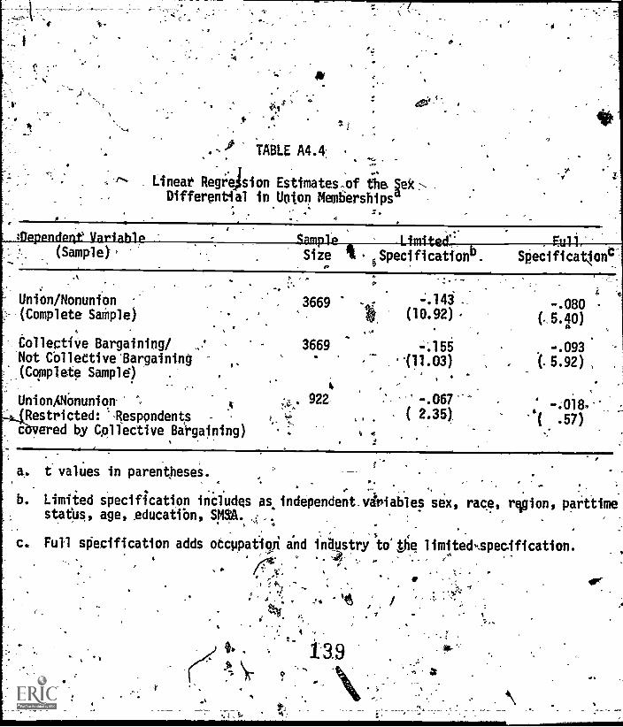
sr

TABLE A4.4-,.

Linear Regr4sion Estimates,of the 5ek.Differential in Union Memberships

(Sample

Union /Nonunion

(Complete SaMple)

Collective Bargaining/Not Colletive'Bargaining(Complete Sample)

UnionANOnunionRestricted: ',Respondents

c`3vered by Collective Bargaining)

Size iSpecificationb. Specification

4

3669 -.143 .

(10.92) ,-.080

(. 5.4,0)

3669 -.155 -.093

111.03) (.6.92)

922 -.067 -:018,.'( 2.35)

''( .57)

a. t values in parentheses.,

b. Limited specification includes asindependent.vbiables sex, race, nylon, patttimestatus, age, educatibn,

c. Full specification adds occupation and inaustry to.the limited-specification.r

(*:1:.1

* ,

Or

.

The Determinants of Job Changing Agtivity Among Youth

CRAPT&R 'V

4t

. -.

. .

Frequent job changing is a:central characteristic of the youth labor,- e 1

markeet., In the past, the proportion of 18 to 24 year olds who change jobs

.

has been at least twice as high as. for the population as a whole.' Other

data Suggest that newly hired workers are much more likely to change jobs

than more experienced workers, with a sharp increase in.job stability when

theindividual has been orrthe job a fear or more.2

_Researchers disagree on the desirab*lity and implications of this turn-,:

over: Some argue that the high turnover rates among youth are the result.

of a useful process of gathering market information. Before long term job

commitments can be made, information is needed on both sides of the market.

New workers and employers hive imperfect information about each other, which

only.direct contact can remedy. -Workers must learn about woricingtonditions

and future prospects with the firm; employers have only limited. information

on the-actual productivity of newly. hired workers.3 With sufficient flexi-

bility in thedNrms,' ability to adjust wages and working conditions, mis-

. matches can be rectified by renegotiating employment contract's. Otherwise,

separations frequently occur; both workers and employers must search for .

improv0ed matches. rn this setting turnover is desirable, facilitating an

improvement in the worker-jOb match.

140"t

so,

. 117-'

.Contrasting with this view is thet argument that much of the turnover

in the youth labor market is random and undirected.. In other words, turnover

is excessive and seriously aggravates.the probleM of high Unemploymerit.

Hall (1970) presents the argument quite clearly:

labor force have rates of unemployment that are far in

excess of the rates tha't would accord with the hypo- :

thesis that the unemployed are making a normal transition

frokone

to be, p

o another. :Some groups exhibit what seems

ogical instability in holding jobs. Changing

from one low-paying, unpleasant job to another, often

several times a year, ds the typical pattern of some

workers: (p.389)

,Unfortunately, choosing between competing interpretations of the pur-

posiveness of job changing activity in the -youth labor market is hampered

by a lack of solid:empirical evidence. In this chapter, we begin our

examination of 'this, issue, investigating the determinants of turnover in

.

the youth labor market.

5.1 A Model of Labor Turnover

In competitive labor'imarkets, rionCompiensatin wage differentials erode .

overtime. Wages increase for workers ceceiving less than their potential

and fall for those earning more. Frequently, however, existing differen-

tialS cannot be liquidated if workers remain at their current jobs. Nominal

wages are often inflexible, particte.,arly downward, and an 'individual worker's

141

.e"

productivity at the current job may be lower than at alternative jobs. 'In

such instances, labor turnover becomes impOrtant to the efficient operation

oof the labor market.

The turnover response of workers to wage differentials has been exten-

118

4 ir

sively analyzed, with researcheri typically relating, industry quit rates to.

interindustry wage differential`' The general findil of this research is '

a negative relationship between quit rates and wage differentials, suppor ing

the contention that the wage structure stimulates a desireable (more effi-

.cient),allocatiop of resources in the labor market. That is, workers move

to jobs where their capabilities will be effectively utilized. Empirical

4

studies of the determinants of layoffs have peen more limited, concentrating

on the role of such factors as firm-specific human capital and union member.

ship.5

4A limitation. of most empirical studies of labor turnover is the use of

current wage 'as the major incentive variable. gob) within an4d among indus= ;

tries, workers differ in their productive capabilities and, in a Competitive

market, wage rates vary among Workers to reconcile these productivity

differences.A As Parsons (1977, p, 207) notes in his recent survey of labor

turnover studies, "the quit probability should be negatively related to one's

current wage relative,to the mean of one's alternative wage distributiod..,

qbut]....on1y information on cur4ligt wage if, dirtctly'observable and available."

..

.

What is needed, given(tbe hettrogeneity of workers arid_jobs, is a worker-,

Specific measure of alternative opportunity.

In the preceding chapter,. We developed the' concept or the maricet

differential--the gap between a worker's current and market or potential wage.

-.

142

AN.

.4

119

The market differential is a measure of alternatives, conveying information

to both worker and employ r. To a worker, it indicates the potential increase

or decrease in wage rates he could expect if he changed jobs. To.an,e4.mptoykr,

the market differential indicates that a gap exists between the worker's

current wage and the market rate. MaxiMizing behavior by workers and

101,

employersimplies that nelOtive market differentiali (market wage greater.than)

current wade) Will stimulate quits, and that, positive differentials will

encourage layoffs.

In idditiopito the aarket differential, many other factors influence

turnover decisions. Workers consider nonwage characteristics of the current

job and costs of changing jobs; employerS Consider severance paymentS' and

hiring costs. Both groups are influenced by the potential loss of firm-specific '

human capital,& and the state of aggregate economic conditions.'

Equation (5.1) describes ajmodel of job' turnover, that incorporates some

of these concerns:

' .TURNi (a, a + 1j = TURN (Ma, Za),

a = age at initial survey,

a + 1 = age at subsequent survey,

TURNi(a; a 1) = the probability of turnover alternative jbetween age a and a + 1 (the four alterna-tive forms of turnover considered are:.QT = quit, LO = ldyotf, OH otherjcb changers, and SJ job steers);

market differential at age a,0

= yvetor of othercurrent.job and situationvariables.at age a.

143

(5.1)

120

Turnover activity is described by four mutually exclusive and exhaustive; .

variables indicating that a worker*quit his job (-QT), was 'laid off his job

(fit) }, 'was_discharged or left:his job without repbrting a reason (OR),,or

remained at his job (SJ) during the one year period between surveys. Each

turnover variable assumes the value 1 if the alternative occurred, .0 otherwiSe.

If multiple job changes occurred,)the reason for t'he first job change dominates.

Also, :Layoffs returning to the same employer are classified as job stayers.?

Details on, the operational specification of the market differential

variables are presented in Chapter IV. The other explanatory variables are

constructed froni responses to specific questions from the survey at the initial

age And include: years of tenure at the current job; years of 'ed tiRn cunt-

pleted; dichotomous variables indicating that the respondent is black or

married; and the set of market opportunity variables indicating the year in

which the respondent was the relevant age.

2The turnover model.is estimated using multinomial logit analysis, where

the dependent variables are the alternative turnover activities. For each age, 40/

the sample examined is respondents the requisite age in any survey who were

employed as wage and salary workers in that and the next year's .survey.

Resliondents the reqUired'age in the final survey year '(1970 for males and

/1971 for females) are excluded since we cannot observe subsequent turnover.

activity. In addition, males the required age in 1966 ire excluded because

the 1967 survey did not obtai:n,any information on reasons for job change's.

Besides including a worker-specific incentive measure, our analysis

differs from most existing turnover studies,by examining all turnover,

delimited by type, in a unified framework. Also our use of individual

144.

4

)7,

121

microeconomic 'data to estimate the model complements the extensive an'alysis'.

of labor turnover using industry data.8

I

5:2, The Determinants of Job Turnover 6.

Table 5.1 describes the variables, reporting the mean values by sub

sequent turnover activity at ages 18 and (24 with the sample disaggregated

by sex. Maxim.= likelihood estimaieslof the logit turnover model's para-

metersfor the age 18-19, 20-21, and 24-25 iterations are reported in

Tables 5.2 and 5.3. The reported estimates use the instrumental specifi-

cation of the market differential variable--that is, the difference between

the predicted human capital (or*potential)

wage and the predicted wage when structural variables are added.

Because only three of the four sets bf'coefficients are uniquely defined,

we adopt a normalization rule of setting the job stayer parameters equal to

zero. The reported parameters thus indicate the effects changes in indepen-"

dent variables have onthe relative probability of a given turnover activity.

Derivates evaluated at the means are reported in' Tables 5.4 and 5.5. The

derivatives reveal the marginal effect ofz,a change in the independent variables

on the absolute probability of a given turnover activity, in the vicinity of

the sample means. (For a more detailed discussion of logit, see the appendix

to Chapter III.)

4

Among our more_ nteresting findings are the following:

Market Differentials

The market differential has a -igitisf..icant negative impact on the quit

decision for males. Assuming mean values for tile other variables, the age 24

results indicate that for a worker with 420'percent positive differential\

415

.

the probability.of quitting .14. If the same worker had.a 20 percent

:negative differential, his prObibility of quitting would rise to .20.: In

other words,. moving from a differential about one standard deviation below

to a differential one standard deviation above the mean (MD24fias a standard

' 11"11 1 111.111 in b about

43 percent.- For young males voluntary turnover represents a purposivew

416,

either specification of the market differential variable.

response to economic incentive. .

Females are another matter. Here the impact of the market differential

on the quit decision is usually insignificant. The coefficient does, however,'

become more negative with age. The voluntary turnover behavior of feMales

thus appears to be much more undireeted than that of males. Examining the

--\effect voluntary turnover has on wage change in Chapter VII w411 help

clarify these conclusions.

11A

Our expectation that, positive market differentials would increase the

probability of being laid'off is not supported by the data. For both sexes

and at all ages, the market differential has an insignificant impact on the

layoff decisions of employers.

If we replace MD with the residual specification of the market differential

REDID, the results are -not qualitatively altered; the level of significance in

the quit equations increases slightly. For example, at"age24, the derivatives

(and t-values) of RESID are -.06 (2.41) for males and .05 (1.63Y for females.

rIf we replace MD with the traditional incentive variable used in mobility'

studies--actual wage or its logarithm--the estimated impact and level of

significance in the quit equations are substantial* below those obtained using

146-

Our results can be compared to Mellow (1977), who estimated a similar4

model of labor turnover With data taken from the NB'survey of middle-ageo

males. The major difference in methodology is that here we stratify the

sample by age. For the middle-aged males sample, the market differential

has a. slightly more significant negative impact on the probability of quit-

'Ong and a: highly sign4ficant positive impact on the probability,of layoff.

The fact that, for a given market differential, older workers are more likely

to be 'raid off is somewhat surprising, given that employer's turnover costs

are probably hiller for oldep workers. One possible explanation for the

result is th1a t the market differential is measured with more error for younger- 4fe

t young ages the measured human capital vector is more homogeneous

and 'implicit purchases of training opportunities may be larger than for

workers in the older age range. Measurement error in MD would bias the

estimated impact of market differentials toward zero in the turnover model.

Job Tenure '4

The year -at- current job variable serves as a proxy for firm specific"'

.

human capital, nonpecpniary benefits, and the general agreeableness of the

worker-job match.9 Consequently, it is not surprising that by age 20 job tenure

is the, dominant explanatory variable in. fhe model, significantly reduCing the

probability of each turnover alternative. The strong showing of the job

tenure variable coincides with the results of others.10

Race

Other things equal, blacks do not in general have significantly higherA.-

turnover probabilities. In' interpreting this result recall, however, the

'rather specialized nature of our analysis. We examine young worker's, employed

147

124

in adjacent. surveys. Workers leaving their current jobs but notsmployed

at the time of the next year's survey are excluded from the analysis., as

are workers still unemployed.

It is also important to remember that here we are examining turnover 0

to studies such as Hall (1972), who extmines,the impact race has on the

probability of becoming unemployed. Only a small portion of job chariging

results in unemployment and as we will see in the next chapter, this pro'-

portion varies systematically by race.,

In a study somewhat similar to our turnover' analysis, Flanagan (1974)

I

used the- NLS young men's datto estimate separate models of the probability

of quitting and being laid off. His procedure is much the same as ours.

First, he estimates a potential wage regression. He then includes the

residual from the wage regression as an incentive variable in the turnover*

analysis. His specification of the potential wage regression differs frbm

ours in two 'important ways: he excludes race as a variable and intludeTt

industrial and'locational variables. By including structural variables in

his potential wage regression, Flanagan implicitly assumes that a worker't

.alternatives are limited to remaining within his current Jocation,and

industry, a:.seemingly overrestrictive assumption, Our alternative treatmentap

of_race simply represents a difference in approach. We inclu race in the

potential wage regression for two reasons: to control for unmeasured aspects

of human capita .and to isolate differentials not related to race,. such as

A

market encla es And Osequilibria. The saire 's true for our- treatment of sex..

148

.1

7

Since we have purged the market differential of its racial (and sexual)

components, we consequently enter race (sex) as separate variables fn

the analysis,.thus identifying their impact.on turnover.

Given this difference in specification, Flanagan finds that being black

has a significant, posi =tive impact on layoffs, but no detectable impact on 11--

,)quits. His wage residual variable has a significant negative impact on

quits; am ignificant positive impact on layoffs. He interprets the

neg#tive coefficient of the wage residual in'the quit equation as indica-,

tidg that "the effect of wage discrimination and occupation segregation

is clearly to raise.the probabiTity of black quits" (p. 23). By including

a control for race (or stratifying the sample tw race), however, Flanagan

removes'ihat component of the wage residual he is most intereste41n. In

contrast, our approach explicitly introduces the racial differential.

Education, Marital Status, and Sex,

Education and marital status have little effect on turnover excest amon

18 year old males, where education significantly reduces the probabil of

quits and layoffs, and marriage increases the Probability of all job changes.'

Estimates of the sex coefficient using the.combtned male and female samples

- (reported in Table 5.6) indicate that females arse less likely to Be.laid off

or to quit, and more likely to change jobs for other reasons. However, the

'reason- for -job- change variables are better identified in the male survey,

which may seriously bias any inter-sex comparisons of type ,of turnover

activity.

X49

4

Aggregate'Economic Conditions

Mat opportunity variables, wh ich co -trol for variations in aggre-

../

v -

gateeccnomic conditions by indicating the year respondents were the rele-

, 126

Vant age; ally refer to turnover actiOty during the next calen ar

or women.1.1 Over the iod 1966year for men, during the current

to 1971, unemployment was initi,all'y "Taw, moved slightly lo and then,

, 47

, beginning in 1969, increasy,drapatically. Since aggregate data reveal

that quits decrease yoffs:inc, rease as economic conditions deteriorate,A.,..

it is not-surprisin findignqicant positive coefficients of variables

fir 1969, 1970, and 1971, in the layirf equations (Even where the coeffi-

cients are not-statistically significant, the 196 cOefficient is generally.7

I

larger than the 1967 coefficientafor men; 1970 is larger than 1969 for women..

Somewhat surprising, however, is the finding that the,probabilitjt of quitting9,

significantly increases after 1968 for women.

1. -. .

5.3 Selectivity Bias and the Draft.

One shortcoming of our analysis of-job turnover is that we eliminatee

espcndents who are not interviewed or not emplpyed.in subsequent surveys./

\, .

Many of these respondents were males drafted into the armed services during\

the Vietnam War. Before concluding, 'efJyexamine what effect exclud-

ing these respondents (who are not random ith loardto individual

)°C racteristics) might have on results reported in Section 5.2.

,

. .

Dail on 18.year old malltwere-aaminee.to determine some of the

characteristics of igodeavees who were not employed in the subsequent survey.,

..,

. ,

Observations were classified according-1,6 their most.Orobdble reason for

.....''Y : .

4 % Vo ..

1

150

4

becoming a job leaver. The only respondents included in this tabulation

were those TritevieWed-in the subsequent'survey (at age 19) who were not

employed and those not interviewed because they Were in the armed ervices.A2

Sepenty-five percent of the 285 job leavers were in the armedLservices at the

time of the'second'survey.

A turnover ldbit model which includes the four alternatilies of the

job change model, presented in the previous section, plus a fifth alterna-. .

tive for the 285 nonemployed job leavers, waSesitimated. Being marriedf

-, . significantly reduced the probability of being in this groupno other fnde-»

4:

pendent'vari.ables Were' significant, and coefficients4for the other activi-.

4' 7_ ties were virtually unchanged. Thege findings do not necessarily indicate ..

i

. ,. 1 .

that the estimated job,change parameters would have-been unchangdd if the

draft had not removed Most of these job leavers from the survey, since there-

is some indicatAnThat the draft overselec ed. the poor and black." But

'the fact that race, and education do not serve as good,predicrir's of leaving

suggests that the-bias may be imall-

Conc/usions

In t101 chapter we examined some of the determinants of turnover in the,

, ..

youth labor market Our major findingscan be summarized as follows: For

males, market differentials have a significant negative impact on the pro6abil-

,ity of quitting,:and ariInsigniffcant impact on the probability of being laid

'off. The turnover behavior of females is not significantly affected by market

differentials. Job-tenure tsasstrong deterrent to,..any type of turnover,

'while being nonwhite or,married ha ro significant independent effect. Con-a

'trolling for other.faators, females, are ths-,. 'ikely than males to quit or be

151 .

. t'

laid .off, and more likely to chgnge jobs for other reasons (although. here

the results are probably at least partially spurious because of data problems).

Finally4 a deterioration in aggregate labor market conditions increases the

Chances of bring laid off.

Our findings' indicate that for males voluntary turnover in the youth labor".

market represents an explicit attempt to improve espnomic.position. 'Males who0

quit are those who receive less than their markeewage. For both sexes,

.utisatWactory-job matches appear to bean important cause of youth turnover;

-- .

. the accumulation of job tenure rapidly diminishes the likelihood of changing

jobs. It is-noteworthy that job tenure is the only variable for which.wel

observe a clear,-age- related variation in its impact on'job chipging. This sug-*

gestS that An initial period of random search 'in the l4bor market quickly

gives way to a more systematic pattern of job_changing-activities. However,.

an obvious limitation ofthe analysis is that we have only examined the deter-.

minants of turnover, not its economic consequences. 'In succeeding chapter's

we attempt to overcome this limitation by incorporating turnover 6ehaYior into

investigations of unemployMent and changes in wages betw en adjacent surveys

(ages),

L.

r

ti

1

4

3

.k

e k

a

:Footnotes to Chapter .1/. , ,

e.

'Bancroft and Garfinkle (1963) report that.23:-.4--fieremt-1-0-11,P4142,

year 7:-P1CI.M4re workers and 24.4 percent :of 4 to 24 year old.. male. workers

.

dinged jobs in 1961 comparf to 10.-T-pertent of all male workers.,

c

ee Crfinkle (1964).

3See Spence (1973) for discussiOn of the importance

teristics 'as. "signals" 'in labor markets characterized by

4See ;.pr example, Sioikov and Raimon (1968)i Burton

encayel (I'M); and Parsons (1972);I

of worker oharaq-

uncertainty.

and Parker (1969,

5See (!arions (1972) andMedoff '(1976). For a recent survey of labor-

.

turnover-studies, see Parsons (1977)."

6To therextent that firm-specific human capital is correlated with the-.

interaction terfn in ,the Stage II wage regression y in equation '4.4), the

instrumentalspecification of the market, differential nets out an average

return oh' such i'n'vestments. . ,

. I , , ,, ,

d .

7For a dftailed discussion and analyiis of. temporary,layoffs--) thoqe

. .

returning to the same employer, see Feldstein (1975, 1976).. In _light of ,,

,

Feldstein's (1975) finding that approximately ,85 percent of all la. yoffs return

to-their prior employer, studies. that use industry data td estimate layoff. -0, ,

, .

equations. (Parsons; 1972, .and Medoff, 1976) are analyzi the

determinants of "temporary" layoffs:.

X

/-

Y 8Other recent efforts using individual microeconomic data. to investigate

,

labor turnover includeHall (1972), Flanagan (1975) and Barte,1ana Borjes..(1977) *

k

9We,do not contfol for all determinants of job changes. Inoaddition,'

tenure ,itself is cpnditioned by turnoverbehaviOr. Consequently, to the...

extent that the allobselwables are correlated with.job tenure, job tenure

becomes a proxy for the unwsdred factors. For a discussion of the impli-

cations of this prdblem see Heckman arid Willis (19i7).

.11See footnote 10 in Chapter"-IV.AC"

130

.

4

12Otber noninterviewees are excluded because-ft could not be determined*

whether they left their prior jobs.

13For a fUrther discusslon, see Kohen and Shields .0977).

4

,_

TABLE.5.1

Variables Used in Turnover Anal4isa

Variable OesCription fdaie

Mean Value by Dependent Variable Category.

Age '18Female

-OT 1.0 OR SJ QT LO . OR. SJ

MD

CJT

EDUC

.RACE OP

MST (D)

1467 (0)

1968 (Mc

/969 (D).

1970 (D)

0

Market differential

Continuous year's of ens-

k;ploymelit with current

or last employer

Years of formal educa-tion.completed

*... .

.

v Respondent is. nonwhite

Respondent is married,r

rRespondent was indicatedage in 1967 .

Respondent was indicated'age .in 1968 '

Op

Respondent waswas indicatedage in 1069

.

:Respondent was indicated

.

-.03

4A45

..35.

.16

:11

,

.44

.39

--r 0,

0

(-

' 0

.33

--..L..e

10.97

.. .37

.1#,

.27p

.30r

.43

--

'

4.,

f

,,,

-.04

.30 4

11.47

..4j

.17

.704.

, .15

.16

0

.28

, 11.63

.29

.08

.34

.35

.31

.04

:27

11-.8

.

.31

.16

....

::,

..23.

.39

.38 .

..;-

.01

. .06

li.56

.25

.06

.19.

.38

-.02

.22

11.54

' A" .27

.34

.25

, .43

.32

'

.02

.44'

_l1.44

- .24

.13

.46

.21

.32

age in 1970

155 '

156

V

f.

TABLE 5.1 CONTINUED

Variables Used in Turnover Analysis

Variable

MD

CJT

EDUC

RACE

HST .

1967

1968_

lk 1969

-1970

Mean-Value by Dependent Variable.Category

Age-24Male

FemaleQT - LO OR QT OR SJ

-.03 -.01 -.03 .01 . -.02 -.05 0 .01.

.97. .50 .52 1.90 . .87 .52 .66 2.40

12.18 9.93 11.12 12.38 12.93 12.82 12.53. 12.75

.73 .30 .35 .21 .31 '.36 .31 .23

.65 .66 .71 .71' .61 .64 .64 .62 ..

.33 .39 .65 .38

.42 .290

.17 .35 .14 .18 .18 .400. AI

.25 .32 .)8 ..27 .32 .45 :27

- -'.73 .33

a. The alternative liePendent variables are: QT, quit last job; 10; laid off last job; OR, left last. job for other reason; SJ, remained at last job.q. Variables followed,by (0)., are dichotomous. They assume the value of 1 if'the indicated requirement is met, 0 otherwise.c. Omitted in estimation.

158A,

a

TABLE 5.2a

DETERMINANTS OF TURNOVER ACTIVITY: AGE 18, 20, 24 MALES

Variable9

tmo

Ca

EDUC

RACE

MST

1967

1969

Constant

N

X2

Ratio Index

AGE 18 AGE 20

n tP04241:31OR

[Mtfi Nx2 (d.f.) {Plr'13 la fmtfigl in 414144 X2 (d.f.)ln{Prr. la S in

-.858 °..018 -.983 3 (3) -1.649 -.116 -.934 12.23 (3)

(2.05) (.03) (1.27) (3.42) (.16) (.92)

.166 .058 -.002 5.70 (3) -.232 -.309 -.211 8.30 (3)(2.36) (.46) (.01) (2.27) (1.79) (.99)

-.140 -.202 .022 11.45 o , -.081 -1.00 :049 5.16 (3)

(2.62) (2.17) (-20) (1.80)..

(1.52) , (.47)

.084' .171 .691 4.78 (3) - .027 0 .150 ..579 1.63 (3)

(.49) (.61) (2.13) (.11) (.44) (122)

x.635 .663 1.004 11.55 (3) .295 -.089 .A5 2.36 (3)

' (2.59) - (1.86) (2.29) (1.36) (.26) (.64)

-.921 -.015 1.673 35.25 (3) L. -.060 -.236 1.898 9.51 (3)

'(4.10) . (.04) (3.89) . -(.24) (.52) t2.99)

It°-.011 .511 .148 3.01 (3) :30T 1.156 t460 11.33 (3)

(.06) (1.69) (.27) (1.29), (3.24) (160)

e .

.403 -.366 -4.262 10.79 (3) -.405 -1.334 -4.847 11.73 (3)

(.62) (.41) (3.11) .(.66) (1.46) (3.18)

1027 722

101.67 (21) 68.54 (21).

.olis , .054 .

1596,4

TABLE 5.2 CONTINUED

Variable

- AGE 24

.1131Pi-obr .21241i *_011

Intprob

SJ afpr---j-90x2 (d.0.9

-1.014 -.321 -.821 4.14 (3)(1.99) (.40) (.69) 0

-

CJT -.322 -.656 -.633 37.86 (3)(4.55) (3.92) (2.41) -

\ .

EDUC -.049 -.2S7 -.147 ° 24.88 (3)(1.36) (4.85) (1.76)

RACE -.099 -.192 .280 .70 (3)(.38) (.51) (.50)

, t .

MST. -.121 -.001 .233 .52

_.

(3)(.54) (0) .42)

1967 -.369 .108 1.125 5.93 (3)(1.54) (.27) s's.,(1:69) s

1969 -.277 .168. .135 1.51 (3)(1.06) (.39) (.16)

Constant -.083 1.098 1.871 . 5,48 (3). ..g,

(.16) (1.53) (1.50)N 700x2 (df) 99.42 (21)Ratio Index .089

a. Reported coefficients, are maximum likelihood estimates of the, parameters of a multinomdal logit model.The alternative dependent variables are defined in footnote a of Table 5.1. The absolute value ofasymptotic t-statistics appear in parentheses. The x2 statistics reported in each row test the nullhypothesis thatall parameters estimated for a giveeindependent variable are zero. The x2 statisticsreported at the bottom of the table test the null htfp.ps that all parameters (except the constant)are zero.

1

111111.11..

TABLE 5.3a

DETERMINANTS OF TURNOVER ACTIVITY: AGE 18, 20, 24 FEMALES

$

Variable

* AGE 18 AGE 20

Protur} .,_{Pro

proLDM fPr__ob11)11)}in

{ pro, cur i protH4ts*/ ProtiAEQ}, In. tProt1) " OJS3) " 'rol:) x2 (d.f.) Prot (5%.1) inro Prob (SJ) e 01.i."

CJT

EDUC

RACE

MST

1969

1970

-Constant

N

x2 (df),Ratio Index

.335

(.59)

-.157

(.93)

1.18_5-

(1.721)

.281

(1.17)

.363

(1.18)

1.294(4.63)

.841

(3.05)

,

.

-.266

(.20)

-1.914-(1.32)

.028(.11)

-.170

(.28)

-.860(.81)

1.250

(1.64)

.561

(.73)

-1.064

(2.66)

-.385

(2.87)

.088(1.14)

.022

(.12)

.116(.48)

1.247

(6.22)

:482

(2.43)

\9.48 (3)

9.77 (3)-

3.45 (3).

1.6213)

2.24 (3)

47.18 (3)

12.40 (3)

-.734

(1.08),

%.371

(3.22)

.153(1.60)

.256

(1.01)

--.481

(2.01)

.296

(1.03).

.351

(1.31)

. _

'

-.318- (.27)

-.553(2.16)

.005

(.03)

.872

(2.04)

-.3t8(.64)

1.074

(1.72)

1.094(1.84)

. -.111

(.22)

-..834

(8.16)

-434(.54)

.029

(.15)

1281

(1.58)

.813

(4.04)

-.071(.34)

'

1.31 (3)

72.03 (3)

3.68 (3)

5.35 (3)

4%.

6.10 (3)

17.80 (3)

5.49 (3)

-4 yrr(3 13) .

-3.715(1.24)

-1.769'

(1.88)

'

II .75' (3)

84391.52 (21).051-

(2.80) (1.68)4 .134

1.16)11.27 (3)

873155.67 (21)

.084.

162-163

TABLE 5.3 CONTINUED.

r -"

Vartabl&

1.

gouc

alACE

LIST

1969

fp2142.3.11.Pro"

-.822(1.09)

-.463(4.41),

4t.041

AGE 24 ,t.ro t0,)

1PlA

ro S t

Prob R .,

(1.01) (.80)-1.600 -.485

*.

-.702(2.19)

I.

,

0

'4.

e,

-.627 56.92 (3)(6.48) 411

v

..037 .. -.008 .66 -( )1.67) (40' (.16)

. ,

.253 ? .483 .175 1.09(.76) -,- 1.72) .( .,64)

\--- :- a . n, .050 , .199 .0811 .19 (3) ,(.16) (.30) (35)

( 1.2-.277

.

1.259(284) .x. (.22)

. .,

(4.02)a

.

20.91 (3)

(3.40) (Liz) (2.17)

Constant

xo2-

-Ratio tadex-4p

-2.715.

(2.90)

413:

-4.053(2.10)

-.965 .11.74 (3)

0

522

. 136.02 (21),.139

' " : ' ,. Reported coefficXits are Maximum likelihood estimates of the parameters of 4 multiaomiallogit model.

The alternative dependent 'variables are defined in footnote a of Table 5.1. The absolute value of"asymptotic t-statistics appear in,parentheses. The x2 statistics qported in each row test thenullhypothesis that all parameters estimated for a given independent-variable are zero. The x2 statisticsreported at the bottom of the table test the null hypothesis that all parameters (except the tonstant)-are zero. :::, .

1 r'd

A

1

IndependentVariable

CJ,T

T

-1967

1969

_t_

a

0

Table 50

-.Derivatives Evaluated at the Mean: Turnover-AnalysisMales Ages 18, 20, 24

a T

Age 18 ' " Age 20

'Prob(QT) Prob(L0),p Prob(OR)..

Prob(SJ) Prob(QT) Prob(L0) Prob(DR) Prob(S

-:i24'

. 224-

Ir

4

:002

, .

-.026

-.001 .

. 0

.f36-

-.025

-.240

-.030

.014j

,.015 -.004

.241

.049

I : 7:00 . .002.

.015

.-.021

-.040

-.015

-.103

, .082 ,

!

. 008 It

.031.

.031

.uti

.026,

.004

-M35

-.139

.085

-.026 (

0.

044.

-,015

;030

.008

:-.009

-:016

.1166 ,

.013

.006

.046'

.008 .

4,

t .

. 1

'- 1654

ti

Table, 5.4, continued

4 or

rndepedltentVariable

Age 24

. PrOb(QT}. Prob(LO) ProbtOR) " Prob(53).

r

MO -.140 -.006 ( -.009 .153

CJT -.040 -.021 -.008 .069

EDUC -.005 -.009 416RACE' -.014 ..004 .016MST )m .00.4

1967 .006 '

1969 -.008

.017

.003'

-

4.

'44

4!"

I

I

4

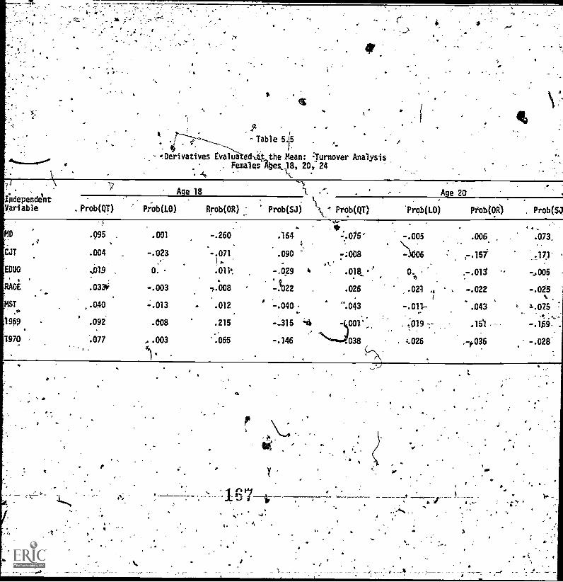
Table 5 5

...Derivatives Evalua edtigthe.Mean: ;Turnover Analysis,. Females iges 18, 20, 24.

t

IndependentVariable

Age 18

Prob(QT) Prob(L0) Rrob(0R) Prob(SJ)

CJT

ENO,

RACE

1451

.0,

196

1970

..

g

,

.:,

.095-

.004

.019

.033r-

.040

.092

'.077

.001

-.023.

O.

-.003

.....013

.008

,.003

4)*

-.260

-.071

-

.011s,

1...008

.012,

.215

'1.065

.164

.090

-.029

-p022

.

-.040,

-.315

-.146

:

*Ati

'

t

'

Prob(QT)

",,,,

-.005 .006 . .073...

.)006 ,-.15i .171

p.15

.7.015 -4005

.021 , -.022 -.025/ A.

- .011 -- .043 , 1.075

.019 -,-- .151 -- .109..

4.026 .1.035 -.028

Age 20

'Prqb(1.0) Prob(OR) Prob(SJ

,,-.075'

7;008.l'

.018 .

.026

..4.043.

.

.038 .

IP 7.; ---4

t.

t

latele-5.5 continued.

Prob(P):

1,1D-;.

CJf

EDUI

RACE .019

", MST1.

.003

1969 .093,

,1970 .115

-.147

-.006

O. 4,04V

.005

.002 '

.7.007

.013

-.516

-.079

,-.002

.019

,011

'.156

4169'

4

-.197

1:2. 3

10144.6

yen An4101s: Combined Staple

DEltamMum15 of TvimOTtx ACTIVITY:

'AnnaAt'l 13

" Pob(S.1) .

',aftrub(tekVroblbJU

,toltreld0r11

sytob(d.1)) %2 MC.)

h.mai= ...610

(1.22)

-.892

(1.. 10)

4.418(5.54) '

36.94(3)

111) -.163 -Ion -.536 10.99(3)

(2.05) ( .23) (3.02)

065,a5:

-.230 6.55 (3)

I i.41 (2.13)

-.160 .029 7.38(3)

(1.34) (2.40)- .( .47)

IAD N. .220 .147 ,162 2.92(3)

(1.32) ( .59) (1.04)

SEX -.212 --1.033 3,320 152.31(3)

(2.891 (11.45)

-DST .532 .407 .333 ' 9.05(3)

(2.111) / (1.24) (1.39)

N77 -.696 .108 2:071 49.46(3)

11.17) ( .23) (5.92)

,_

1129 .432 .757 . .960 36.65(3)

''(2.83)

4i.75) (5.36)

IC°

.477 .583 .420 7.66(3)

(2.09) (1.06) (2.17)

Leg likelihood52 (d:l.)

AGE 10 AM' ACE 20 SAYILInla,"

T;FiT011tob(5.1)

(1.54)

...733

(3.62)

-.311(4.03)

-.046(1.24)

.123

( .71)

-.213

(1.13)

.346(2.16)

-.0211( .10).

.329(1.31)

.392(1.61)

.4738.96466.67(27)

ACV 20

In/N.0.01 ,

(nrob(9.1)

. ,

-1.685 3.485 21.113(3)

(2.04) (4.59)

4..167 -.153 1345(3)( .51) ( .71)_

-.398 -.764 78.29(3)

(2.77) 0.07). ,

-.075 ....Ott° 2.83(3)

(1.24) ( .16)r

.432 .006 3.00(3)

(1.64) "( .03)

+% -.217 41.740 103.30(3)(2.76) (9.41)

-.149 .292 7.56(3)

( .54) (542) 6.,

-.219 2.054 19.62(3) Ne;/'( .50) (4.34) '

1.176 803 30.37(3)

(3.32) (4.26)

1.193 -.050 9.28(3)

(2.59) ( .24)

" frag)1 1' (d.i.)

-1451.21,463.43(27)

. tr 44

.

a. 'Reported coefficients areftiwaTikelltood estimates of the porsaascaza of a saltine...lel logic model. De alternative dependent

variables are defined Is toote a. to Table L.1. The absolute 'SIAN 0( elyUcCOCIC [-statistics appear lo parentheses. The 72

statistics repotted is as roe test the WU hypothesis that all perimeters estiessied for 4 given lodeperdent variable ate zero.''"

De z2 statistics reported at the bottom of the table test the mill hypochesie that all parameters (except sheet:messes) sts zero.

DE*134119E5 EVALUATED AT THE NEAR: AGE 111 MD ACE 20 3433925

it

TAR1ASLE

AGE It .

hob (0) trob(1.0) trob(01) treb (SJ)

ND -.ill .002 -.043 .085... ,

Err :om , :wag -.023 .010

SD ' .00931 .

" .006 .005 .010

it t".: .0p .010 -.043

Ea -.SS .054 421. ; 4173

OIST .071 ger .071 1.011 ..100

111)7'.146 .001 ..062

MD! . :041 - .023 .olf: -.742.

1100CO .058. .014' .028 .401

Prob(01) Prol.(10) Prez(01) 1r06(h1) .

-.001 .099

: -.062 .100

-.003 .011.

-.003 402$

. 444. -.206

.021 ...OS/ 4.

:1$6 .....133

.062 -.121

7.016 -.077

-.097 -.0011' 4

-.027 -.011

.005 -.003

.0144 .017

-.024. -.024,

.o4 -.co 4

.OS/ '..018

.024 .044

.046 .04$

1

169a

$91,:

Chapter Vi

Duration df,Unemployment Among Job Changers

As doCumented in Chapter 'II, youth unemployment is.disturbingly high.

In this chapter we examine someb of the-determinants of unemploYMent durationa

. for those workers in. our samples who change jobs between adjacent ages. We

confine our analysis to.this restricted sample for several reasons. FiAt,

within the context:of ow. recursive framework, unemployment as an intermediating

activity.in the equilibrating process deserves separate study. Second,,

we are unable to determine completed, duration for: respondents still unemployed

at the time of the second survey. The major consequence of our selection

procedures is tlieremove new entrants and re&rtrants from the analysis. Sihce

these. two.groupe constitute a significant proportion of unemployed youth,1 thei

......

possible effects of excluding them Should'be kept firmly in mind. Complementing

.1 .

the age-stratified,analysis of duration,. .the chapter also co tins in investi-

/.

gat on of the unemployment experiences of malesraged t8-24 n 1966 over the

1,9 6 to 1970 period., .

'*

.

/6,1 Job Search, Unemployment Durationand liarket Equilibration' ...-.

The economics of job search contends that searchis aN-oductive, infor. /

nation generating activity. It is/1-topicithat hasl.stimulated Considerable

theoretical research, but only limited testing of key implications. One

.

important impiication of theoretical models of job search..is that a reducticm

in the cost of search increases the optimal amowt of search: On the assumptiona

that the duration of a spell of unemployment can serve as a proxy for the amount

of. search activity, several researchers have examined the impact that measures

of search costs such as net assets and nonlabor income have on durkion; manyr.

.,more have inyestigated the efiect,that unemployment insurance has on'duration.3

170

143

711

f'

If differential search costs affect search activity; the link between

a worker's Search 'costs, duration of unemployment, and subsequent wage rate

is direct. All else equal, the worker With low search costs searches longer. ,

.

andbtains a wage that, on average; is in the upper portion of his wage4

distribution; he has a positive market differential, Con versely, the worker1

with high search costs engages in more restricted_ search, accepting employment'

t arwage that on average is in the lower pOrtion of his distribution; he has

a negative market differential. If search tosts.are correlated over time,

the market differential.would thus be an inver'4e indicator of present search

costs.'

df .

At the initial job,_search cost (dis)advantage determine (firnarq)who .

hash negative and who has positive bifferenti -; However, the component of4c-ef,,..,

,7-,,-----

the differential attriblitable to differential search costs is not stable.

Profit maximizing employers compensate workers int- their productive capabili-

ties, not for their search activity. Consequently, employers are not hesitant,

about trying to liquidate positive differentials. Wo kers located in low

wage jobs because of high search costs are continually' oking for ways to

improve their economic position., In a labor market dominated by long run

competitiire forces yet characterized by costly information, two opposing

forces a-rttius at work: "market equilibrating forces stimulate the liquida-

tion, and search cost (dis)advantages contribute to' the. maintenance a7 existing, .

wage differentials., In *this chapter we exathineAuration ofiunemployment among.

job changers. 'Assuming search costs ars correlated over time, the interpreta-, . 'ty.

tion'sketched above5 suggests that workers with negative differentials move, ...____

I, 4 it ,.

quickly though the market changing jobs with little or no unemployment: On. .-

r '

the other hand, workers with positive differentials who are forced into the

market search longer, atteinting to maintain theirexisti ng.premiums.

', . ,

. ,..3 . .- k.,. ..y,... ..,, . . ..

,

Consequently; a negati/e relationship between the market differential and

duration of a subsequent unemploymentspell is expected.6

A major problem that needs to be considered before we proceed to outline

an estimating equation is our use of unemployMent duration as .a proxy for the

amount ,of search actiyity.. Despite the fact that they are frequently identified,

.as such duration pf unemployment and the amount of search activity are not

synonymous-7 The unemployed usually to not engage in full -tilde sloth

activity1847,In addition, a substantial'portion of search activity may take ".

place at.the prior job. Although we lack information on the intensity of

'search while unemployed, search at the'prior job appears to. be quite substantial.

As fndicated by the data presented in Table 6.1, Only,a .small minority of the

job changers in our, samples. experienced any unelipii;ymett..L_Eor_maDY change-ft.,

duration of unemployment thus appears to be a poor proxy for search activity.

A partial correction (for this deficiency is to control for differences in the

reason for turnover. As Table 04-indicates, a higher pertentage of laydffs4%

experience some unemployment between Jobs. We hypothesize that layoffs engage

in less search at the prior job than

In addition to the market differential and turnover variables,,the,set-t

of explanatory variables used in the duration model includes a vector ofi

, 0

personal characteristics (race, ,sex, education, current job tenure, and, , . -. ,

. maritrl status), and the market opPOrtunity variables*(to control for

vridtions in aggregate economic condiitons). .Equation (6.1) summarizese% ...-

fhe model.

a.

Da,.a / = 00 * 0 mn e 'TURNa, a +:-,-.3`M0

.4 $4 PC +

where

a' = age at ITITtrall'survey

a + = age' at subsequent survey 172

1

41,4

'ry

4

A4S

Da, a + 1 = duration of unemployment between ages aand a + 1,

MDa = market differential at age a,

TURNa, a + 2 = type of turnover between ages a and a + 1

/ (alternatives are quits, layoffs, and other),4

mo -= vector of market opportunity variables,if. %,

PC = vector of personal characterittics,

c =:stochastic error term.

6.2. Em i cal Findin s

F

The duration model,is estimated for the sample of respbndents who were

the requisite age in any survey, were employed as wage and salary workers in

that and the next year's survey, and changedjobS between surveys.10

4

Respondents in the final, survey year are exc we, since no 1 orma ion is

available on Subsequeni'duration. Unlike the turnoVer analysis, males the

required age in 1966 are not excluded; 'their reason'for jobthange is coded-

"other."

Table 6.2 describes' the variables used in the analysis, along with their

mean values: °Tables 6:3'through 6.5 reported regression estimates of the

duration model for the ages 18-19, 20-21, arid 24-25 iterations, with the

sample disaggregated by race and sex. For expository reasons, we refgp, o

the initial age in discussing each iteration. ,Thus, for example, t g

.18 to 19 iteration is called the age 18 iteration. The basic results can be

4quickly summarized..

Market Differential

For the combined sample, the market differential-,has a significant positive

impi5t on expecte0 duration in the age-18 and 20'iterations, but n6 detectable.

impact in the age 24 iterations Its impact, is uniformly for males than -

4

for females; greater for black's than for whites. At age 18, a 20 percent positive

differqni41 (one standard deviati above the mean) implies increased 6nemp'oyment

1 73 .

146.

between job changeS of slightly over one week for an otherwise average

11male..-

The finding that the market differential does not -have an especially

robust influence on duration is .not challenged by several experiments not

reported in the tables. -If we substitute the residual specifjcation RESID,

the level of significance typically declines by aboLli 5 percent; if we limit

the sample to job changes with reported duration,of One week' or more, coef-.

r4

ficients are always insignificant..

Expected duration is shorter for quits than layoffs., usually by two _

to three weeks. Younger males arethe group for whom beirfg a layoff increases

unemployment the most. A problem with this part of the analysis, however,

-

is that ,the l'eason. for job.change variable is Often poorly defined.

Aggregate Economic Condttions

The econ&ic downturn that began in late 1969 has a verydroriounced effect

on duration.of unemployment. Changing jobs during 1970.ihstead of during 1969

was as-sociatJd with a two to three week increase In. expected duratiOn for, both

males and females. iNOte that the market opportunity variables actually-refer

to unemployment during the.next calender year for men, during the cureent.year

to

for women; see Chapter IV,Yfootnot410.)

, Personal Characteristics

,,;In each age regression,blacks,experience longer duration of unemployment

thartwhites, with the magnftudeof the gap increasing from under one week at

age 18 to over two weeks at age 24. Females have about a two week increase4

in expected duration, with the greatest increase at agg 24

The impact of education'and current job tenure is poradic.. Being married

reduces expected duration by slightly more than One Week. The relatively poor-

. r ",

showing of these variables is consistent with finding's:of other researchers wto

have estimated duration of unemploymenimdels far young workers. (Stephens*

,

.

0976, and Ehfenherg and Oaxaca, 1976)..7i."14-

1'

147'.

6.3 The .Unemployment Experience: A Long Run Analysis

We have thus far examined the determinants .of uneiliployment between jobO

changes. This section provides an alternative; complementary view of

unemployment in then youth labor market. Restricting the sample to all

nonenrolledmale'wage and salary workers aged 18724 in.1966 who.were alsoI.

employed in 1970, regression models of the total. num14er of unemployment

spells and the total weeks of unemployment over the four year period are

estimated. Explanatory variables are defined as of 1966 and include -the market

differential, years education, marital status, years at current job, race,

plus age. The results are summarized in Table.6.6.

The market differential has no detectable impact or either the incidence

or duration of unemployment. Surprisingly, neither does age.12 Educatibn

and current job tenure reduce both incidence and duration by proportionate

amounts, while being married has no impact on incidence but a strong negat40

ct on duration. Blacks have a significantly higher,inctdence and duration.cmof u ployment, with the duration effect being larger.

'®Some hypahWcal calculations provide an indication of the magnitudes

involved. All else equal, a black with 11 years' of education can expect\1.413V,

unemployment'spells lasting a total of 7.09 weeks; for a white with 13 years of

education these expectations-decline to .65 spells and only 3,697weeks

.unemployed.

6.4 conclusions

Although the scope.of our analysis in this chapter is limited; its

implications are important. The generally positive impact that the market

dtfferedtial has on duration of unemployment provides limited support-for the,

hypothesis that those with lower search costs (positive market differentials)

search longer.' We also4find expected duration lower among quits, whites,%and

females. Finally, aggregate economic conditions have a tremendous impact on

175

a fob changer's expected spell of unemployment. Alin else constant, an 18-year

old thee changing jobs in 1970 could expect to be.unemployed over 4 weeks

. longer than the same 18-year old changing jobs in 1967. For a 24-year old,

the difference is 2.7 weeks. Complementing the age-stratified results, analysis

--of the unemployment experiences of a fixed Cohort ()versa longer period indicates

.

that blacrs and.the less edudated experience much more unemployment--both in

incidence.and in duration of given spells. These results for wage and salary

workers are consistent with the findingi reported in Chapter III, which analyzed

the labor market \actiyities of the full sample of NLS respondents.

;

1.

176

1

1

.

Footnotes to Chapter VI

-

BLS data'on reason for job change indicate that a large part of teenage,

,unemployment can be traced to a pattern of frequent entry and, reentry into

thelabommarket. In 1975, for-instance, the proportion of the teenage

labor force unemployed because of labor force entry and reentry was 14.5

percent cOmpated to an. overall teenage' nemployment ratd of 20.5 percent.

For youth ages 20-24; however, entry and reentry, are much less important as

reasons for unemployment. In 1975, 4.8 percent of the labor force in this age

group was unemployed because of entry or reentry, compared to-an overall group!'. ,

unemployment rate of 14.6 percent. Th6se figures-are calculated from tables

3 and 4 in Hedges (1976,I; similar results are also reported in Perry (117).

2For' an extended review of the various tVoreticallmodels of Sbb search,

see the recent survey of fLippman and McCall.(1976).

-3See, for examples Stephenson (1976) and Ehrenberg and Oaxaca (1976).

4Although the NLS does obtain information on proxies for search costs

such as net assets, nonemployment income; and unemployment insurance benefits,

.

there are severalTroblems with using these more direct measures of search

. - .

costs.

to explain duratioh of unemployment. Asset and income data appeatil'to 0

-,

be unreliable and are only collected in selected years. In addition, measures,

, .%. J

oe..search costs such as unemployment insurance benefits.are jointly determined

with theduration of an unemployment spell.. ,

5For a more extended development 6f the argument, se e Mellow (1978A

. 177

.6If the implicit assumption,that the searcher has perfect ktiOwledge of

150' '11

4 .

,:his wage distribution A not satisfied, a worker's market diffeential might

be positively)'

relatedoto his perception error. .If, far instance, 'a worker's

.2

, positive differential is pure rent (as, .for examOle,returps to a

.

p.otected enclave), he may not recognize that he was paid more than his market

'worth and initially overestimate his wage distribution. 'Ad9pting an 4

9

. sipappropriate search strategy would thus result in a pos4tiverelation between

".., ,. the market differential and subsequeritduration. Lonsequently,lo, 0 --/ ..,

,the extent *that perception errors are common, we may 'erroneously,

r , .. .

co Jude that-the data show areiatio between search costs and, duration

ll

S.

1 .

w in f,kt the,relation egtithated has a 'different-interpretation./*

.14

, . ^ 1,44.

7McCal--1 (1970 ,makes the identification Clear at ,the outset: "The amountED ,-

of search on'the peHod of. unemployment...," (W. 114). (emphasis added); others, . 4'

' k-k

: .

----.

are less' rect, A e;410 1970), ftir example; accepts'the possibility of search.t,

l,

O 4-

at the prijarjob:bdt sa.rgu s that since Search As more Oficient ,whe the job

seekerik.Aemployedwr, as,he:puts self- employed in the -full time.

.

accumulation of infoitationthe job seekerA11-.voluntai7qivv e unemployed.

le , , . e

8For eviclehce`on this,point',,see Gordon (1973) and Barron anOtellow (1978):

...,......_.

. ..

... ,

. ,

,. vThis.- .oberiied high percentage of direct job ChaAgers,.particuTarly among'. .

, 'quits, is consistent. with earliqr findirigs.'

MittiTa (19744;for example;,

,

., . . .,. ,

presents estimatels,-obtained from a wide,array of data sdurces'(colleCted at+

,

t "I' .s.., 4.. 6 4, ' ' .

Nariousj*intsAn the businegs,cycle and "across variop.demograOkic groupings),

'Itip V. 1k ',1

. c

thaf indiCate mat least 50 AO 60 pe6cerit'of all,quits. move from job to job:Withr%

,

N,

, . .

. out evet'experiencing,unemp.loyment." (p. no

4

4 44 04 V

IP*V.!

ft

.44

.

O

a ;-

.

i

o'

, 4

*4 ;. o

omitting- respondents still unpmployeit at the tfinie of tfie'sUbsequent

,

survey, we are truncating the distflbution of upe010,1nent-duration. There

. ..

,,.

'Hare obvious problems of selectivity bias associated with.

thi&.procedure.

-

. ...

7 -

Most.other studieS using N data to examine unt'nployment ddratioil'also have

this limitation; see,lor:i ce Ehrenbeh and OiXaca 9976),

. : - .,

,

., - -,

In their anafysi;of unemployment duration usirig"NLS youth data,

. ...

Ehrenberg and Oaxaca (1976)-includgd severaT direct pioxies for search costs,.

Of theqe, only the coefficient on a °variable Measuri ng unen1O1 oyment insuralCce. .

16.. benefitswas ,significant. Recall our earlier commenti(footnote 4),that there

maybe possible simultaneity problems here, haever.,

12The simple INNmelation,Otween age and education sample:isthis sample_is only .

T. -

:

4

f'f

*- 179'

4.

.

- Table 6:1

Job Changers Moving DIrectly0to a New Job WithoUt Any Intervening Unemployment,. - By Reason for Job Change: Agds 18 - 19

7

,

Reason Fork;aving,

e .18 Job

Total in Group With No, in GroupMaking,Total in Group Reported Unemployment . Direct JO Change

, 1... ..

White NonWhite White Nonwhite .White ,Nonwhite White Nonwhite White Nonwhite White NonwhiteMales Males Females, 'Females Males , Wes, Females Females Males Malep Females' females

_

Layoff

Putt, a

Other

All4Job.

'Changprs

a 1 4-ji,,, . . ,.4 ;

. .'a .

. t , , t.

.a.. In each survey,individ..als were asked the amount of unemployment expuienced (in weeks) /luring the preceding 12-mcinths: For job changers

thereportedduration of unemployment is attributed to the job chang. This, assumes job changers. not reporting any (one week,orimore)

'

o...,,, .

.4

242

. *IF V.P; .

. .45'- . 29 12 , 4 31' 18 . 8 0 . 68.9 62. 66.7, ..0 ..

I'-. -.

. ,i' .-I -

149 74 83 37....118 57 . .,......E, 26 - 79.2'. 77.0 73.5 70.3 ,

,

88I

45 '220 BO, '68 .. 31 140 43 77:3 68.9 ' 63.6-- 53:8

"%...,

,

I

. l''S:, l Pa .4.... I..... . 4.,

148 , .315, 121 217 1051.20.9

77.0 r' 71.6 966.3 57.0

..0

t.

E.!

unemployment moved directly to,tpe new job.. .

/

A

'a

ft

A-

181.

/

. /. 1140 .

Jr -

1,4

a

r

.4_ 'Iv

TABLE 61,2 ro

..1

. Variables Used in Duration of Unemployment Ahalysis

to,

Variable

I Ma-

:QUITa. a + 1 (D) a

LAYa, a 4. 1. (D)

A,prIERa, a + 1 (D)bb

1966 (D).

1967.(0) ,

. 1968 (D)b

1969 (D)

,

. .1970 (D)

." EDUCa .

0 .MSTa (D)

- CJTa.

1...; :NE (0)., k

s''

..WKUWa ; '42., ir..o. .L

Descriptioh '

.,

. '

Ages 18, - 19'

Mean

.. .Ages 24 -- 25 .

,

/4

Male Femalp Male Female.

Market differential age age a,

Left job at age a boause of quit'e

/ ,,,

Left job 'at age a ecause of layoff

Left job at fthage a other, reason.

Respcin4dent was age a in 1966..,,

Respondentoyes age a in 1967

Respondent was age a in 1968

Respodent was age a in 1969

Respondent was age a in 1970

Years of formal education completed

_..

C

-.019

7 .519 .

.172

0.309t

.258'

.200

.272

.270

.....

11.24

L.902'

. .275

.037

, .688

.241

.417

.34?

11.55

-

/

.

,

'-.023

.525

.196

.279.

.246

.288

.271

.196

11.58

-....0.11

.42

.060

..61r

_.,--

- 17d-'

.385'

,445

12.68

,.

`b

.

...

. NMarried at age a

-

Continuous years of employmentwith .cukent or last employer

...4 Re,spondent i's nonwhite

1 .

Weeks unemployed between ages..a and a + 1 .

1

.147

.1744

.344'

2.81,

i .

;140

'.....2)4

.278

2.43

Ii

.688

- .725

.254

2.31

. '.

.

.632

.719,

At-

.313

2.53

1111-

a.v.Variables followed by (D) are di4C1otomous.Ommitdd in estimat*on.7 , . 40p

r.

They assume Vit value 1 if the indicated. requirement Is met,0 otherwise'.

a5,

183

I.

IndependentVariables

MD

QUIT

LAY

4969- --* ---.'-

1970

EDUC

MST

CJT

SEX

PACE

CQNST11 o

SSE '

1 I*.

t's CS

Table 6.3

Duration of ,Unemployment Regressions:. Age 18a

.3

.076 -.349 -.124 . .

( .32) (1.70 ( ( .69)

.556 4.828 .

(2:31) . ( .65) (1.16) (1.44)

-.081 "-,198 . 2..191)

(1.09) .( .5) (1.00) ( .T6),

^ - .

.- .866

(1.50

.

Niles

(slack tomb'd BI ck

6.658 4;321 5.442 3.287.0.333 (2.69) - (4 \29) (1.20)

-;/. 2:883(1.76)

-.241 1.021- . 23 -1.991( .17) (1.20) ( .85) (1.68) '...

3.185' 4.264, 3.594 .650(1.99) (3.97) (4.07) . . ( .18)..

1:230 1.633 1,20( .72) (1.64 ) 1.75)

',-7.514' -.463 -.427"( .57) (..50) ,( .55)

----.2.957' -2A,404 - - 2-617 --- 1.405(2.34) ,(3.01) (3.84) ( .89)

1.953 4.296 219 4.738.205 . .148 .-- , 54 .107

5.%17' 44859 5.137 5.731148 282 430; 121

?

to,

Fen al

White Comb'd

Combrd.

-.544" . .532

( .40) ( .44)

-.220. . -.692'( .36) (1:28).

-.08 .175

'( .03) ( .14)

2.917.(3.32)-1

-.407L.93)

2.436(3.67)

.295

( .41)

(1.87)

% -Gas, .566' 1.455-----r-( :12) ( .88) (3.18)

2.873 2.971 3.526(4.08) ,(4.53) (6:96)

-.269 -.353 77(1:01) (1.61) (1.4

-.872 -i.347(1.09) (1.92),5 (g.22)

-.077 -.097( .20). ( .56)

. (3.18)

.689 - .716

(1125) (1.84)

5.685 :5.460 4.374-.084- "'" .084 :101

4.669 4.167 5.091 ,

315 436 866I

. a .. . .. .

The depindinteV le %is duratio (t o unemployment in weeks, avdescribed in .

"footnotoie.-to e.6.1. The absolute value of asymptotic t-statistics appearIn parentheses.

. . .

4.

1

,

':.

A 4 .

, ..

* .

4

4

,

Table 6.4

Duratibn of Unpmployment Regressions: Age 20a

IndependentVariables Black

..

HQ' 7.659., (1.58)

QUIT: .-1.592. .44)

LAY 2.451I. S --.. ''-- .58)

1966 S -2.429( .55)

1967 2.081

1969

1970

EDUC

HS;

CJT

SEX

RACE

a O.

# .1

;Hales: Females

White Comb'd Black White Comb`)!'. . \ ...2:928 A.354 ' 5.809 -.987 '1.503

(1.35) (2.15), ., (1,47) ( .59) ( .92)

-2.491 =2.295 -1.377 - .861 -. -1'.'698(1.56) (1.53) ( .78) (1.24) (1.57)

. . .1.071 -.110 -2..774 -.252 -1.262 .

( .58) ( .06) (1.11') ( .18) (1.01)

-.433 -.943( .22) ( .51) -, s.

. ..-52 .63 -. 0 4. - '

Combkd

...

3.190(2.51) , -

-1.561(2.39)

11(

-1.679(1.4%)

:.632-- ,__..59.) .,1,-,1a)- __ C -30 - . .. ( '591

3.817 2.0'4 2.777(1.29) (1.49)' (2.19)

-.186 -.308 ` -.253( .4i) (1.53) (1.35)

-2.569 -.535 -1083(1. ( 52) (1.25)

-.325 -.327( :soy ( .93)

cosT 7.168 'Is,

. ---114- ,,./ - 4.., .106SSE° % 'N. 9.227,

t N . 0 82. ..

1.430 -.940 -.455 ' ° .905( :69). (107) ( .56),, (1.33)

6.259 1.132 2.40.8 ,- 3.224 .

(2-81) 41:44) (2.96) , (3.95)

-.253 -.462 --:43191r--- -.294(' .46) (3.99) .(1.89) (2.13)

1 4

. 4(71 -" . 873 -:4626 -.86Q( .29) (1.41) ( .99) (1.60)

,-..717 -.709' _,5_97 '-;.368( .63) : (1.94) ci.ok , (1.48)

-2.343,

,

1.103(1.95)

0

%*'

4.156..16)

I ; 1:953(2.89)

.

7.814 .269;° 5.379 8.-899 7.880.096". .078 .125 .060

6.678 .41'1 7.877 4.994..088

i5*.973214

is' 296: 119 294 413.

1.0.*

..110a. See footnote a. to Taple

4 4011?

.5

.71

,. 8.011.066 i

- 6.625704..

IS.

-S

w-

M

IndependentVariables

drMD

Os-

.

.!'...-, .

QUIT .',

1967 .

;

'' 4 CJT

CQNST

SEN

.Table 6.5

Duration of Unemployment Regressions: Age 24a.1

4

, ..

-2.448 . -.147 .690 '2.0 .-6.155 -, -2.427 -.698 -

( .75) ( .09') ( ,.46) ( .4 (2.37) (1.02) ( .52)

-1.774 . .372 -.161 976 -2.354 -1.173 a . -1.195-. ( )54) c'.33) C .13) '( -.36) (2-28) '(1.09) (1.58).% ,,

4.5q3 . 3.128 3-362 1..580 -3., 936 .

_.1.856 1.640

(1.40) (2.56). (2.66) ( .131-.. (1.84) ( :88) (1.65)

t'

C .09) ...( .9), ( .42) !III19660 -.342 1.195 .566 -

- ,

3.537 -.275 4. ,- a -.222q.33) "(1; 38)' , ,( .54) ( .24)

--. .

_

2-284.- -,2.352- '2.171---- -3.214 '-.906 -.791 1.106.., ( .82) (2.9.9) (2.46) ( .9.2) ( .60) .54) ' -(1.39)

. - - -.162' 1:689 1.371 29273

( 1 ( .05) (1.10) ''.. (.90. (2.27)

. -.,

. .,, .

..

i .149 -.002 .065 -.254 .318 -096 .065

( .44) ( .0.) ''( ,54) ( .56) (1.70) ( .50) - ( .67)1 I

-1.740 -1.002 a -1.291 -5.065 .286 -1.686 -1.448.,

( .95) (1.70) (2.01) (2.08) ( .29) (1.66) , 2.5210,

1.180 ..041 .242 -1.726 -.321 -.470 . .030 .

(1.72) ( .24) (1.22) (1.34)- 4..98) (1.20- . ( .?6)

Hales 11. Females Comb'd. - .

4

Black- White- Comb'd Black White 'CbmAi

. ....

,-..

.220. .162. 1691.413 . 1.003

.

.479 11.587 -1.744 2.167:132 .145 +.083

2.335.691

S % 6.756 3.944 4.559 8.700 5.172 6.549 5.532 .4 61 179.. 240 57- -125 182 - 422

t .

j2.119

(215)2.235 2.299 -

,' (2.06)

#.4*

(1.70) .

-

16

a. See footnote a. to Tabfe 6.3.

4

ti

Se

r

X

6

Ac

44.

?,`

0

TABLE 6.6

Unemployment Experiences 196611970:Males Aged 18-24 in.1966a

-IndependentJar:fable :

..,

EDUC 11.30 -.115 .

-.581

.r

. ,

Dependent Variable

, .137L .4971

;152

( ..31**)

(4.79) t, ,(4.86 ).

,T .52'. -.076 -1.94

..,C,IT, *,, ' .22

RACE .27

4,

AGE 21.36

( .64) (3.03 )

.

.

k

.,

"(

.

-.126, (3.94 )

.258

(2.03 )

030( .99 )

-

v-..,_..,,

.

.

.

-' .514 4 :-(2.94 ) i...

2.834

(4.09 ).", .

-.03( .24

9

)

.

a. The' sample is males. aged 18-24 in 1966, not enrolled, and employed as wage and salaryworkers who were also employed at wage and salary workeriIri 1970. All Independentvariables are constructed with data from the 1'966 survey. The dependent yariables.are constructed by sunning data from'the 1967 through 1970 surveys. The means are.89-and 4.78 for number of spells and duratton respectively., The absolute values oftAtatistic appear *parentheses.

0

CHAPTER VII

Wage. Growth: The Acquisition of ProductiveSkills and Market Equilibration

I

With this chapter the anaryiis comes full circle, returning i6 the

topic off' wage determination in the yOuth-labor Market. Now, th'e focus. .

of our inquirylis the determinants of wage growth between adjacent ages.

In our investigation, we explicitly examine the influences that market-. ,,,

J,.

,

alterOitives.(as indicated by the worker's market differekjal at the,

4

initial age), improvements in skill levels,between ages, and-changes:,in--,.-k ,'

aggregatd labor market conditions, have on the patternofmagelgrowth. .,

As 'the final componentin our' recursive model, he'analysis also4considers. . .

the. effectshat job change and unemployment have on wage growth.

*

7.1 Thestiage''Growth'Process

The hypothesis that market forceS erode,noncompensatingiwage'differ-

entials is equivalent to saying that a worker's wage change' depends (in.-

,.,

part) on his market differential. Thatis, amorker with adinitial wage.. - ,, .

greatei-. (less) than,:his capabilities warrant will'experience below (above)4

average wage growth.

As discussed in earler.chapte s, turnover and unemployment may'.

intermediatein the wage growth p ocess. Since the market differential

affects tIvbse activities, including turnover and unemployment dUration

in tihet-analysis allows us to distinguish the market differential's impact -'

9t I

on wags growth from its inckireCt7 impactoperating through the di4nnels

of turnover and unemplument.

159

But, of course,` wage growth is much more than-simply an equilfbrating

et. a )phenomenon. Workers 'are constantly adding to their productive capabilities,

,

`and these increases command additional wage paymentA. Young people are

particularly active-in the acquisition of human capital between adjacent.

ages:, completing an additional year of formal schooling; participating

srin. training programs outside of school; and eccUmulating general work

experience. These acquisitions should result in some immediate wage growth,

allbough full-returns are probably gathered Over a period of years.

Accordingly, the initial el of human capital may also influence wage

growth. Finally, changes in aggregate economic conditions may affect wagAP

paths among young Workers.

1,

A description of the wage growth.Orocesi betweenladjacent ages that

incorpOrates,these concerns is represented by equation (M);

ln(WAGEa INAGEa

83 ADDa,

= 00.+ 1 + 82 DGa +

+ 8,, MO + TURNa .

a i

06' P/KU N (7.1)+ e

were,

a = 4age, at initial survey

a'+ 1 = age at subsequertt surveyA

WAGE =, actual wage at indicated age

MDa= market differential at age a

11Ca'= vector of personal,characteristics:atgie a (race, sex, Marital status,

* education, job experience),

ADDa-a. = Vector of variables indiCating

4ntredOnts of education, training, 'and experience added"between'ages..a and a +

189

= vector of market opportunity variables;

TURNa, a 4;1 =-vector.of turnover variables indicating .a quit, layoff, or other type'of jobchange between ages a and,a + 1,

WKUNa, a + 1

= weeks unemployed between, ages a and a + 1, and

= stochastic error term.

160

The dependent variable approximates the percentage change in a worker's

real wage between adjacent-ages, and the market differential variable

measures the.direction and (in pekentage terms) the M'arikude of the gap

between his actual and his market Or potential wage at the initial age. A

negative.coefficient on the market differeptial variable is expected; a

value of -1 would-indicate the complete liquidation of an existing differ;

ential over the one year period between adjacent ages.

For a variety of reasons, however-, we do not, expect complete erosio

of (measured) existing differentials. First, because-of our inability to

fully control for compensatingyariations and subtle differences 'in worker

quality Nt captured by the human capital.varitablesd measured differen-

tials overstate actual differentials. The effect of this overstatement

is to bias downward our estimate of actual equilibration. 'Second, adjust-,. s

men;sjn thelabor market- are not costless: Firths face hiring costs and, .

0

workers moving,costs-if turnover occurs. Because of these adjustment costs,

some differentials will remain even at equilibrium; it isOmply not econo-

-mical to make the adjUstments required to insure complete liquidation.

we, have arbitrarily adopted a one year time horiion, which may--,

be too short for complete equilibration.

13Q

,161

7,2 The Determinants.of Wage Growth: Empirical Evidence

4 ,

For each age, .the wage change model is estimated for respondents in

any survey who were employed as wage and salary workers in-that and the

,next year's survey. As in the turnover and unelployment, analyses, respon-.

dents the requii-ed age in the final survey year are excluded since wetave,

no additional observation on their wage rate, Unlike the turnover analysis,

we do not exclude males the required age in 1966; job changeriin this':e

group are desigliated "oth "

. .

Table 7.1 describes the variables and reports'the mean values at

ages 18 and 24 with the sample disaggregated by sex and race. Regressio'n

estimates of equation (7.1)(arereported in Tables 7.2 tHreugh 7.4 for

ages 18, 20, and 24.

In the wage growth regression, we use tA instrumental specification

%.", of the market differential (equation 2.2c) rather than the residual speci- ';

fication. A major motivation behind our continued emphasis on this.speci-.

fication_of the market differential now becomes clear. The resiOuan speCt-1

fication is the difference between) the log of actual wN' and the log Of

predictediwage (that is, RESIDa --. InWAGLia InWAGEa), GoftseqUetly, anya

error in the measurement of WAGEa is ineluded.in theva0able. BUt WAGEa. ,.- ,. .- .

,' r .is also a component of the dependent variable. Hepce, using RE§IDi would,

..

, .

result in a, spurious negative Correlation wit* he wage 4hAnge vdriable,. .

biasing the,absopte 'magnitude:of the estimate, coefficient downward:, In

. ..

,.

. . C, 4contrast; because MDa is the 4%ifference' betw/er-tWo wage instruments, it j ,

', ....Independent of, any measurement .error in the wage variable.2 'Fina ly., inv

....

*

-t,., . * 1

1

4the reported regressions, MDa is sectored into positive (PMD) and negative

(NMD1 variables.' Employers (workers) have she incentive to liquidate

-positive.(negative) differentials; sectoring the, ifferential into comp-.

nents tests for any asymmetry in'the equilibrating. process.

For expository reasons, we refer to the initial age in discussing each

, iteration. Thus, for instance, the age 38 to 19 iteration is called the

age 18 iteration. Our findings can be summarized as follows:

162

Ma ibrat -ion

The results indicate a strongly asymmetric pattern of equilibration in

the yduth.labor market. Negative differentials are readily liquidated;

positive differentials are not. In other words, workersreCeiving less than

-their market potential are successful in. improving their economic condition.

Employers seem unable to liquidate existing rents measured'in absolute terms,

but average wage growth is low few workers with positive differentials.

Thus the relative poVtion'of those workers in the wage distribution,

deteniorates.

For the full sample (column 7), 47 percent of an 18 year old's existing

negative differential is eroded by age 19. (A negative coefficient for NMD

.implies a positive wage change since NMD is less than or eqbal to zero.) By

*age 20, liquidation*of negatiKed0ferentials increases to.58 percent, declin-

ing to 19 percent by age 24. The market's efficiency at liquidating negative

differentials excepdt its ability to reduce positive differentials. Although

the coefficient of the positive market differential is unifdrmly negative,

it is significant only for the age 2Q iteration.

192

1t'

earned on curf-ent investments. Wage rates of ttioe with above average ain-

163

Equilibration is generally greater for females (compare columns 1 'and 4).

At age 18, for instance, 76 percent of a female's negative differential is

dissipated during the year, compared to percent for males.

.Disaggregating the sample into job changers and job stayers r veals the

importance of direst market contact in facilitating equilibration. For all

job changers (column 8), the coefficients of NMD range from:-.46 to -.67

while the corresponding coefficients for job stayers (column 9) range from

-.04 td.-..45. WitH the exception of the age 18 iteration, liquidation of

positive differentials. is also greater among job changers.

Taker as a whole, these findings, indicate that market forces function

to facilitate the worker's attainment of his human capital or potential wage,

Workers are not permanently trapped in jobs below their capabilities; how-

ever, some workers are able to maintain an enclave wage. We interpret the

market differential varable as representing noncompensfting occupational,

industrial, and locational premiums. Consequently, the obServed erosion

of negative differentials is consistent with the findings of Leigh (1975)

and Barnes and Kohen (1976), that the upward occupational mobility among

yoUnglworkers is substantial. The observed pattern of wage growth, however,

is also consistent with Rose's (1972) interpretation of wage differentials

as representing; differences in the amount of training purchased by younge:7

workers. In the Rosen framework, individuals with zero market differentials, ,t

purchase the average training package offered in the market. Those with

positive differentials purchase less than average training; those with nega-. . ,. A . .

tive differentials, more tian average. In subsequent periods, returns freo

193

J.

faster than average in subsequent years; conversely for workers

with less than average training.

A similar Analysis of wage change:using the NLS middle age data iss

reported. in Mellow (1978b). With an older samgle, much smaller amounts of

training are implicitly. purchased and the market differential variable hat

a clearer interpretation. The results of this analysis are quite similar.

Examining wage,growth between 1966.And 1967, NMD66 has a coefficient of -.19

(t-v4lue 3.52) and PMD66 has.a coefficient of .01 (t-value .14).

Job Changes and Unemployment Duration

The coefficients of the reason fora job change variables arm generally

insignificant. Likewise, unemployment, time does not appear represent

effective job search; It has no systemitic impact'on-wa6e change. The

indirect impact of market differentials (through their effects on turnover

and unemployment) is small. Thus, although our results indicate that youa

in jobs below their capabilities experience substantial upgrading and thai

direct market contact facilitates the upgradihg process, we are nevertheless

unable to detect specific turnover activities directly affecting wage

tg6Wth at the new job.

There are several'possible explanations. Recalling our discussion in

Chapter VI, workers with positive differentials may be searching harder to

'134

A

0

4

. 165

s ksipplyinaintain wage premiums. -That is, search cost.(dfs)advantages help.

determine one's place in the wage hierarchy at the firsejob, and in. Ubse7

quent contacts extensive search' is a mechanism.for maintaining.existin

premiums in the face of liquidating pressures. Alternatively,. unemployment, _ __ _

may not be a proxy for search activity at aTl. Instead, it mighttpeptesent, 0

asomewhat purposeless excursion marked 'by idle time and nonmarket activi-,

ties. -In contrast to the search theory expectation, a negative impact-of

unemOloymenton.mage change wouldthus be expected. Indeed, unemployment

at an early age might permanently scar workers or funCtion as a poOulation

discriminant for workers With what employees regard as undesirable charac-

teristics. We will explore the issue in more detail in the next Section,."

4-where we examine the impact unemployment has on wage growth over a longer

-

Period.

Education, 'raining, and Work Experience

. /The pattern of significance for human'capital variables is mixed..

, Look-

ing at the full sample (column 7),, initial levels of education and work

experience have no .significant impact on wage change (except for a perverse

-result on education in tie age 18 iteration). An additional year of educe-vo

tion OEDUC) andisparticipation in training during the year (DTRAIN) add

4$0

significantly to wages only in the agef20 iteration.

,

The weeks_ worked variable (DEX) IS. significant at ages 18 and 24. The

interpretation of this variable is clarified .by calculating the impact on

wage change of an additional year of employment. For example, mialtiplYing

.

the coefficient from the age 18 iteration (.00f52) b,y_52 weeks, yields' a

7.9 percent increase in wages for a full year of employment..

,

,.

195

4

"K

that a year spent.our of the labor forCe (but not in school or training)

costs an 18-year-old 13.8 cents per, hour in wages'the next year; at the '

observed average wage rate of $1.75. Since.average wage rates rise with*

thevcostiof time spent out Oft the labor force rises.wrth age; for

24 year olds,-the'cost is 21.2 cents per hour. These,results are comparable to

Laiear's (1976) findings 'that, for NLS youhg males, a year out bf the labor

force between 1966 and 1969 costs the individual 14.8 cents per;bour.

Personal attributes (race, sex, marital status) have no significant

impact on wage change between ages. As the analysis in the next section

will show, however, over a longer period of time the wage growth of blacks

significantly exceeds that of whites, a result consistent with the findings

reported in Chapter IV.

Aggregate Economic Conditions

The impact of the market opportunity variables also confirms the results

obtained in Chapter IV. ,Real wages increase'through 1968, and then decline

significantly between 1969 and 1970, dindesfi'y between 1970 and 1971. A male

becoming.19 in 1970 (his market opporturiity variable is l969) experienced

a 6 percent average decline in real wages (column 1), 10 percent if he

changes jobs and 3 percent if he does not (column's 2 and 3). Comparable

fem'ales(.experienced declines in real wages of 14, 18, and 6 percent, respec-

tively Acolumnv-4, 5, and 6). The,susceptibilitY to worsening aggregate

economic conditions declines for older workers.

I

4

4167

The deCline in real wages among young. workers can'be compared to the.

overall' movement in real wages_over the period. Between 1970 and 1971, for

instance, thq average real wage of workers in the private nonfarm sector,

increased 2.7. percent..- Thus, in addition to disQropartionately high unemplay-,

ment durinTeconamic downturns, young workers enc nter a deterioratinY,

. ,

wage position. Consequently, the hardships faced by youth during economic

downturni will be seriously underestimated by lookin'g simply at increased

I e

4

unemployment:4,

7.3 Wage Growth': A Long Run View

, .E amining wage growth over a one year time horizon may be,, too short a _

period to fully capture the cumulative effects of human capital acquisition

and market equilibration. Consequently, to provide an alternative view

of the wage growth process, this section examines the determinants of

wage growth between 1966 and,1970 for a sample of males,employed as

wage and salary workers in both years. The model specification is roughly

equivalent to eqbation (7.1). The market differential variable is the

instrumental specification measured in 1966. The turnover variables are

replaced by a composite variable: the number of unemployment spells

between 1966 and 1970. Weeks unemployed are summed,overthe period.

The human'capital variables remain as befor , only now the initial levels

are as of 1966 and changes are measured over the 1§66-70 period. Age in

1966 is added as,san additional explanatory variable'as is_a dummy variable

indicating the-respondent Was in the armed services., Table 7.5 defines

the variables and reports the results of the analysis.

Ektendingthestime horizon increases our estimate-of market equilibration.' 4 k

''Although we still detect a strong, asymmetry in favor of negative differentialt,5

197

O

4

. 168

the coefficieMs on' both the positive and negative variables are now

significant: Workers iff-T& loge jobs (relative to their skill..levels)

in 1966 substhntially overcome the disadvantage by 1970; more than, 62

percent of an initial negative differential is liquidated over the period.

Older workers experience slower wage growth, confirming the hypothesis

that human capital investments decline with age. As in Chapter IV, we

find that, all else equal; lacks significantly imErovedtheir position

.in the wage distribution dur ng the late 1960's; wages of blacks increased

5.4 percent more than those o whites. Marital status and currett job

tenure in 1966 have no imp wage growth._3

Only three of the ediating activity variables significantly

affect wage growth. The number of spells of unemployment and the _total

weeks of unemployment both reduce wage growth. Two 10 week spells of,

unempldyment over the four year period, for instance, reduce the growth

in real wages by about 9 percent.`' Completinga formal training program

results in a 4.5 percent wage increase. Surprisingly, weeks Worked over. /'"

the period, participation in the a d services, and completing additional

education do notaffect wage owth.

7.4. Conclusions

The bottom line in the wage change analysis is that we do not find

workers ermanently trapped in jobs below their capabilities. For the

mo part, however, we are unsuccessful in directly. documenting specific- 4

#

t

O

labor market activities that encourage this equilibration. Although

'we could not identify any particular type of turnOver as systematically

affecting wage change, we do find that the liquidation of existing.

-differentials 'is greater for.those workers having direct market expindre.. .

198

169

As,in other parts of our analysis, we find that decIlning aggregate

mic

.conditions severely disrupt the youth-labor market, in thit

.instance calling a halt to any upward-movement in real wage rates:

It is.thelpuhgest workers in our sample who are most affected., Fihally,

when vie analyze wage change over a longer, period, we find that increased

unemployment over the period is _associated with a significantly Tower

final wage.

Q

199

,Footpotes to Chapter VII

1Possible sources of misspecification of tile market differential are

diicussed in chapter IV.

\

2Spurious correlation is a.problem co f9und in studies using

microeconomiclongitudinal data to estimate the effect that a worker's .

initial wage position has on subsequent change in his wage rate. Ehrenberg1

and Oaxaca(1976) and Taubman (1975), for example, examine the impact that

.

current wage (earning;-) has on subsequent wage (earnings) change. Using

NLS data (all cohorts), Ehrenberg and Oaxaca estimate a 1966 to 1967 wage

change equation that inclddes 1966 wage as an independent variable. Using

NBERThorndike data, Taubman estimates a 1955 to 1969 earnings change

equation that includes 1955 earnings as an independent variable. Both

studies find that current wage (earnings) has a"highly significant negative

impact on wage (earnings) change. Because the market .differential .is a

component.of current wage (earnings) this "implicitly supports our hypothesis

that'there is dynamic liquidation of existing market differentials. However,

_since current wage (earnings) also contains 'a measurement error component

that is spuriously correlated with wage (palings) change, the estimates are

biased in a negative direction ana i unclear what implications emerge.

.

Norkers'with positive market differentials experience slower wage

growth than a5erage; those with negative differentials, 'faster wage growth.

The following tabulalion for 18 and 20 year old miles shows a substantial

difference in mean wage change of workers grouped by market diffeiential.

20Ol\

171

Differences-are less'signifitant at age 24.

Average Wage Growth at Age:.

Sample18 20

t/Hour % Change N t/Hour I Change N

Full Sample 18.2 9.8 1344 20.4 \ 9.6 936.

1 .

MD < 0 23.0 14.2 665 37.61

i 19.5 435.

MD > 13.6 ,5.6 679 5.5i

1.0 ,501

4Limiting the analysis to males aged 18,to 20 in 1966, estimated equilibration

is larger ( the coefficients of PMD and NMBHare -.406 and -,746 ) and unemployment

experiences have a stronger negative impact on wage growth (the coefficients on

the incidence and duration of unemployment variables are ,-.021 and -.004 respectively)

4

2O

1

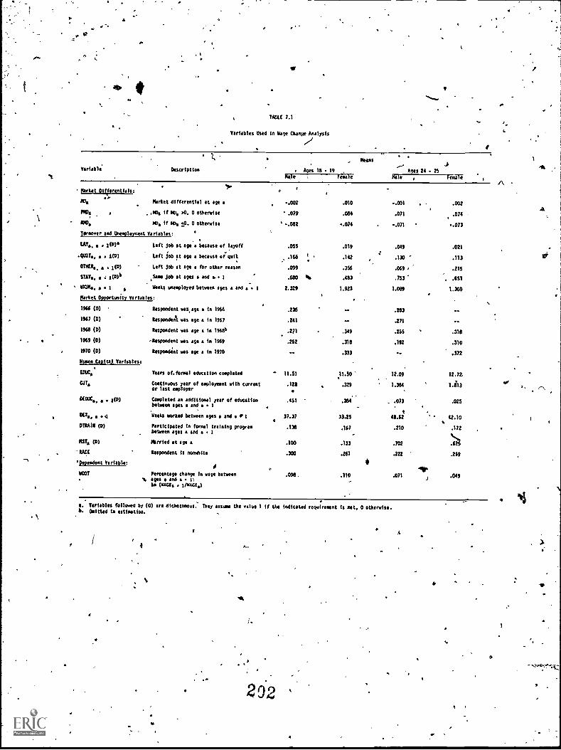
TAU( 7.1

Variables Used is Rigs Change Analysis

a

fariable7 Description Ages 18 19

,

,

Means

Ages 24 - rsRale Of e Rale ,

A, . ".Market Differentials:

-.002

.079

-.082

.055

.166

.099

1

.010

.064

-.074

.019

.142

.356

-.001

.071

-.071

.049

.130 -

.069.

, .002

.074

..073

.021

.113

.215

MD.a..

Market differential at age a

9M0. . JO. If mu, w). 0 otherwise

NM. 40. If mci. .0. 0 otherwise

Ts/sower and Unesoloymant Variables:

SAY.. , 1(0) left job at age because of layoff

40744 a j(D) Left Job at age because of quit

OTNENa. . 1(0) left Job at 190 for other reason

STAY., . . 7(11)b xSess job at aged a and I .680 Rs .483 .753 . .651

WICUM., 1 Weeks unemployed between ages a and a^. 1 2.329 1.923 1.069 1.308

Market Opportunity Variables:

1966 (0) Reiser:dist wansge in 1966 .236 - .283 --

1967 (0) It/sonde:t was age a in 1967 .241 -- .271

1968 (0) Respondent was age a In 1960 .271 .349 .255 .318

1969 (0) .1mspondent was age a In 1969 .252 .318 .192 .310

1970 (0) Respoodint was age s In 1970 .333 .372

}(saes Capita) Variables:

ADM.' Tears of.foraal education cmpleted 11.51 11.50 12.09 12.72.. . ,

CJT. Continuous year of employment with currentor last employer

.128 .329 1.164 1.1113

DECOCa. a i(D) Completed an additional year of educationbetween ages a and a I

.451 . :073 .025

tme, 4 Weeks marked between ages a and a 41 37.37 13.25 48.62 42.10.

OTRAIN O07 Participated in tarsal training programbetween ages and 1

.136 .167 .210 .172

g.'MST. O07 Married at age a .100 .133 .702

-RACE Respondent is non bite .803 .261 .222 .259

'Dependent Variable: *441

(I

MT Percentage change in wage between .110 .0711

.049. si. ages s and a i:

In (=Es 1 /WAGE.)

I. Variables followed by (0) are dichotomous. They assume the value 1 If the indicated requirement is met. 0 otherwise.b. Omitted in estimation.

V

4

20'2

O

.

L

4

lAtAC 7.2

1434 Change Regression. Ages 111',.

.

841es Feaslet Corbined *

.

'S

,

/4714410

11.1Y .JC JS Att " 4C JS ALL JC JS

(1) (7) (3)14) (5) 1(6) (7) (8) (9)

Parket pifferentisl

PhD -.112 .032 -.183 -.176 -.181 -.069 -.18111,412) (.14) (1.57) . (1.06) (.79) (.91) . (1.39) (0) (1.74)

NO -.268 -.517 -.118 -.755 -.771 -.638 -.467 -.654 -191(2.62) (2.54) (1.01) (5.78) (3.83) . (3.87) (5.84) (4.67) (3.06)

, / 1Tunwer end Unsmo Ionwat

t QUIT -.003 -.136 .45 -.017 .007 '-.064(.11) (2.19) (1.03) .(36) (.29) 11.67)

--

. :LAY -.047 -.167 -.101 -.160 -.111 -

(1'.03) (2.19) (.96) \(1.36) (1.10) (1.90)

0110 .111 .056, .069(2.93) (1.70) (2.11)

5913% R .003 0 .004 -.001 -.002 -.002 , .002 0 .003r(1.32) (.03) (1.75) (.33) (.34) (.46) (1.03) (0) (1.42)

8148Ret Opportunity .

1964 .C42 -.018 .066 -- - .036 .018 .057(1.31) (.25) (1.98) (1:19) 1450 (1.71)

1967 .062 .107 .042 r- .047 .105 .037(2.10) (1.60) (1.13)

4 (1.66) (1.70) (1.21),'1969 -.069 -.096 -.037 -.135 -.178 -.095 -.145 -.044

(2.C4) (1.59) (1.15) (3.66) (2.95) (1.34) (4.25) (3.57) (1.6?)

1170 -- -.017 Z.028 -.001 0 -.Olt -.014(.48) (.45) (.03) (0) (.36) (.36)

Users apitel end Primal 1

Chiricteristies .

IRO -.017 -.020 -.013 -.009-

-.018 -.037 -.016 -.018 -.014(1.28) (1.53) (1.45) (.66) (.89) (.38) (2.45) (1.58) (1177) ,

. .. .. .

OJT .014 .C42 .006 .013 .056 -.026 .016 .03 .001(1.36) (1.21) (.41) (.63) (1158) (1.02) (1:76) (2.16) (.07)

IC= -.023 -.002 -.033 .031 -.027 .064 -.005 -.018 -.004(.12) (.04) (1.111 (.94) (.51) OM/ (.27) (.51) (.19)

001 .001 .002 .001 .002 .031 .032 .033 .001(1.76) (.91) (1.09) (2.53) (2.78) (1.11) (2.76) (2,70) (1.17)

871.41e .046 .036 .054 .010 -.002 -.002 .036 .025 .035(1.47) (.66) (1.40) (.25) (.03) 1.04) (1.49) . 1-64) (1.12)

..096 -.112' ..C47 -.024 -.077' .033 -.070 -.097 -.0444,,(2.621 (1.80) (1.911 (53) (1.14) (.96) (2.49) (2.1$1 (1.25)

, PACT .031 .063 .006 .014 .037 .02$ .047 .020(1.26) (.48) (.24) (.44) ci81 (1.13) , (1.48) (1.04) (1.03)

SIX -- .. . .. .016 .074 0(.69) (1.06) , (0)

.2111 .355 .201 .111 .285 .097 .158 .241 .15S

.OSS .097 .035 .094 .129 .081 .C40 .103 .034SSE .378 .414 .341 .410 ..454 .351 .352 .444 .3511344 '410 514 843 / 436 407 2187 866 1321

a. The d49endent ylrtible lt the nitvrarlegarlthe it the ratio of the wafter.% (dellete4) wig* St.agt 14 to the (deflated) rip it age 19. OwlOptolvt4 value of 4sprotbtic itAtiStiti sooner le parentheses.9. AltenItirt smiles 1nc1voe Att, 411 employed es wige and Salary workers teen 11 and when 194 JC, these who clwinged Jobs 4etwetn 6944 18 484 leiAM{ J5 these nee remlne4 at UN in Job.

4

203

5,

Variable

I4

partet Differential

PM):

,

,

lirsorefind 1.1neloal.ent

. .

At

01161

14.

ti

7A6LE 7.3

.

Vag, Mingo Regression: Agei 20 - 21s

..,

Kates faults '. Cabinet,

ut ' 4C JS ' ALL JC 45 ALL 4C 45

(10) (11) ;(12) . (13) (14)Q

(1...9../-

-.361 -.063 -.129 -.074 ,=.249 -:496.. -.1'46

(2.97) (;:931

"

4f (1.46) (.53) ' (.50) (.41) (4.53) (2.63)7 (1.33).

-.609 ' -.631 ..662 -.329 -,453

(4.30) (2.33) (2.110) '(4.62) (2.99) (3.2S) )v0 . j(jl24)

. . . ... I

(16) (17) (16)

6

.073 -.054 -- .041 s .016 .006

(2.05) (.62), . (1.04), (.34) (2. 1) (..14)a

-.612 -.109 :022 -.032 - -. -.026

(.23) (1.08) (.31) (.37) (44) (1.38)

.644 -..

, 042

(.66) 1 (1163 (1.. 76)

.o.

-.COS .CO2 .004 l'Ai7'.002 -.001 -.002

t -ice

'Witt Opportunity

.

0

(2.35)

.016(.46)

.010(1.17)

,

..055(1.40)

(1.61)

IP

-.139(7.31)

-,097(1.25)

-.173(2.37)

.-

.1960

1961

41969

10

INNS CSpitai sod PersonalShareetertstles . 4,

-.001(.20)

.013(1.39) .

.065(2.60)

.0

(.07)

.06(2.36

..04(1.59

02/(44)

414

(2.14)

I .169

(2.26)

0(.06)

.126

(1.33)

-.071

(1.29)

.065

(1.16)

'

'

tOOC ,

KLUX,

1157

,64tE

4.

(1.21) (.34) (1.24) (.12) (1.23) (.44) (1.13)

-1

.045(1.12).

.074(2.02)

-.016(.42)

4..

(1.30)-.097

.041 -061(7.31) (..301

.061

(2.is).

-.061 -.167 .031 -.051 -.137 ,, .002

(1.68) 32.92) (.91) . (2.29) (3.16) (.09)

..-.056 ' .016 -.049 .1.121 ..016

(1.92):t

(.46) (1.71) (2.31) .. ('48)

(.20.082

(1.06).011 .031 -.011 .003. .006 0

(1,27) (.64) (.54) (46) (.03)

7

. -.023 -.027 %..001 .010 ..010

i:(121 .0.'19) (i::1) (2.11) (.17) (.62) (1.26)

.

.051 .055 *.052 .062 .075 .101 .054 .

(1.36) (142) . (.06) . (1.44) (3.06) (2.22) (1.93)

0 .0.262 .022 .001

(:29) (2.04) (1.36) (1.47) (1 );131 (1.06) . (.93).001* .001

. ,

.065 .036 .039 -.017 .067 .063 04)

(1.65) (1.11) (.69) (.42) (2.36) (1.49) (1..)t.028 . .030 .073 -.007 -.007 .011 -.017

(.65) (1.09) (1.60) (.24) (.06) (.36) 1.75)

'C°2 . ;011 .041 -.010 .0111 .055 -.003

(.05) (.33) - (.65) (.30) (.90) (1.52) (.11) .

... .. .. ... .. .. .016 ..004 .024

(.66) (.06) (.90)..

41,

COAST06*

'.652 .134 ..156. -.323 .114 -: -.044 ' .6.035 *4. -.coo'

£2, .107 'r. .227 . .055 .051 .077 .049 .074 "!114 .050

SSC .371 .' .421 .340 .353 .472 .249 .363 .420 ..319

I IA 296 . MA t ' 873 413 440 1009 709 1100 .

*` r . ..

F - ". f

.,.

If 4. Tho itomlett variable is the moral town)* of the ratio of the roratr's (deflated) wag, et eye 20 to the (deflated) le at ege 21. The

absolute .6140 of asyrsototIc tstetrittes appear In 0arentheses. '-.

4 416 Alterastive soles inclose ALL. all ...pivot as wail 4nd salary workers rACT 20 and when 21; 4C. thos6lOy0 cheated loterotween ages 20 and 216 and

4S. those who easfned at the W4 VA. , .i,...

.

' , .......

P204

*43

- Urfable

Cr '

$.41! cif ti

ID. k

Teraever and tateiclognat

UT.

awn _.

..-Ka.., .

/Market Opportunity

1N11

1967

1949

4

1970

Rasa Capful and PersonalCharacteristic,

cadat ...

155 /

r

' 7841.5 1.4

. 42'

Woo ClUngt Regression: toes:24 25

.016 -.045 .036(.65) 1.67) (1.64)

(..CO.007 .007

14) (.12) (.37)

.411 , -.COS 019

(.46) (.18) 151)

..OP

..

'r

Males

fa\ JC JS Ate,(19). ' (20) (21) (22)

-.

...IC° 251 -.055 ..049.(2.00) Cu) ( .ss) (.34)

-.103 -.375 .044 -,331:- (1.32) (1.15) (.55) (2.85)

. .

(114! (01.a22 ,a:11

-4 . (1.02)-.04$

.169

.

(1.74) (2.72).-

(.184)

-.ON - .083(2.23) (2.39)

-.002 , .003 -.032 0(.67) a (.41) (.66) (112)

.083 .271 ,

(2.84)

..

(3.04) (2.33) (

f.039 .107 .021

(1.66) (1.32) (.2.2),.

.001 -.027 .020 -.090

'' (-34) (.35) (.73) (2.64)

.. .. -.041(1.26)

.

'

.001 .031 0(.03) (.06) (.23) (.06)

.002 0 .004 . -409 '(.34) (0) (1.03) (I.)))

033 -.22r .055 .147

(.-.09) (2.03) (1.62) (1.74)

-.001 .002 -.002 .033(.77) (.62) (1.76) (3.41)

(.13.)

.057

(1.51)

.003

-.020(.6Cf)

'-

.074 ...30 .129 -.1044113 .109 .02S .088.261 414 .215 .214

. 970 240 730 122

. resales Coebfaed

JC JS "41.1 JC JS

(23) (24) (25) (26) (27)

.. .

-.235 281 -.039 -.225 .035-, (.64) (1.78) (.48) (1.13) (.43)

-.181 -.110 ..456 -.040(?.90) (1.49) (2.89) (3.03) , (.69) *f

s-.

(:\

-.141(2.24) ,

.042

..

.-

-.0111

(.71) ' (.56)

.096 ,075' (.34) (2.37) (1.07)

- -- .016(.63)

--

'0 -.00 - .001 .002 -.031(0) (1.06) (&31) (.63)

. (.6))

.

111-1,14'' .039 ohs .osi

(1.12) (.06) (2.20),

- .017 .049 - .1:05(.13)- (.26) (.21)

-.178 -.031 -.086 ..014

(2.07) (1.57) (1.45) (1.54) (.66)

' -.071 -.036 -.011 -.037 -.014

(.80) (1.15) (.30) (.53) (.49).

.

-.CO6 .004 0 -.033 .001.

(.50) (.64) (.01) (.35) (.49)

-.036 -4704 -.03i -.012 0(1.65) (.61) (.62) (.94) (.05)

s..163 .131 .038 -.116 .054

(23) (1.50) (1.14) 11.27) (2.15)

.004 !On ,002 .031

(1:S21 (3.67) (2.26) (1.29) (1.74)

44) (.35) (1.09)(43) (2.02) 17(.(1.54) (.76) .28) (.40) (1.64)

-.040 .057 .007 -.014 .018

.021 -.004 -.041 .021(il) (.61) (22) (1.19) (.11)

" .. .02/ .044 .031

(1.12) (.93) (1.34)

.111 .025 .025 .020 .0111

.193 ..051 ' ..020 -.061

.144 .006 - .026 .076 .025

.371 . , .236 .204 404 .231

182 ' 340 1492, 422 1070i *

I. Tho 40.4est variable It UN natural leurItlis of ma ratio of the 4drkes (dsflatad) we at age 24 to the *.

rued) west stilt 25. the absolute rolls or asoptotic t-statistics appear fw parentheses.11. tefutiee Wales itclink att. all uployed as watt and salary workers when 24 and khan 25; JC. these tho chanted Sobs Mittman ages 24 and25;

4411 .14. theta Mao cantata at the awl 105(

2054 ,

TABLE, 7.5

Determinants of Wage Growth 166-1970:Males Aged 18-24 in 1966

oSA

-IndependentVariable

Mean- Coefficient(t - value)

e

Status in 1966:_ ,

larket Differential > 0 .08 -.270(2.17)

Market Differential < 0 -.07 . -.624(5.87)

Years Education 11:19 .014(2.54)

Age 21.36 -.022(3.14)

Race (1 = black) .28 .054- (1.99)

Marital-Status (1 = married) .52 - -.014( 52) AIY

Intermediating Activities (1966-1970):

Weeks Worked' 179.94 -.0002( .62)

Weeks Unemployed' 4.85 , -:003. (2.32)

Number of gnempOyment Spells , ..91 * T.014(1.89) .

Completed Additional Education .07 .062

(Years)° ( .06)

Completed Formal Training Program .46 .045

-41 = yes 0,86)Served in Armed Forces 71 .27 -.012,

. , (1 = yes) (.37)

a. The sample is all nonenrolled males-who were employed as wage andsalary workers in 1966 and 1970. The dependent variable is the naturallogarithm of the 1970 actual wages (in 1966 prices) divided by the 1966actual wag& The mean valueof,the dependent variable is .29. The sampleis 1113; the is ,092; and the constant in the regression is 623.:

A

cp.1

. I

CHAPTER- VIII

Conclusions andTolicy-implictions

The purpose of this study is to provide empirical evidence on thedeterminants

andimplications of various youth labor market activities. The study is Motivated. 4

by a desire both.to improve our understanding of how the youth labor_market operates

and to identify mellower problems that might be addressed by policymakers. This

concluding chapter briefly summa, rizes our findings and examines their possible

implications for.youth labor market policy.

p.1 Summary Of Findings

.6 The central hypothesis tested throughoUt the study is that observed. behavior

in the youth labor market is guided by lorig run competitive forces. Ovr results

provideAxed support for this hypothesis.

The study begids by documenting the flow of individuals into school or work,.

As expected, person's continuing their formal education- beyond high school experience

.a less difficult transition into the labor force, with a lower incidence of unem-

ployment. Among. early entr.ant, to2the labor market, high school dropouts are likely

to experience the,highest unemployMent rates. ,

In examining the Wage determination process,'We find that the influence of

. . -. .

traditional human capital factors is strong and systematic. pucation, training\ .

and work.experience all increase thleworker's expected wage. However, we also find. .,.. . .

. ,

that at any point in time, discrepancies exist between the typical worker's current.

. -, *

and expected wage-- We call' this deviation the market differential \ ,

207

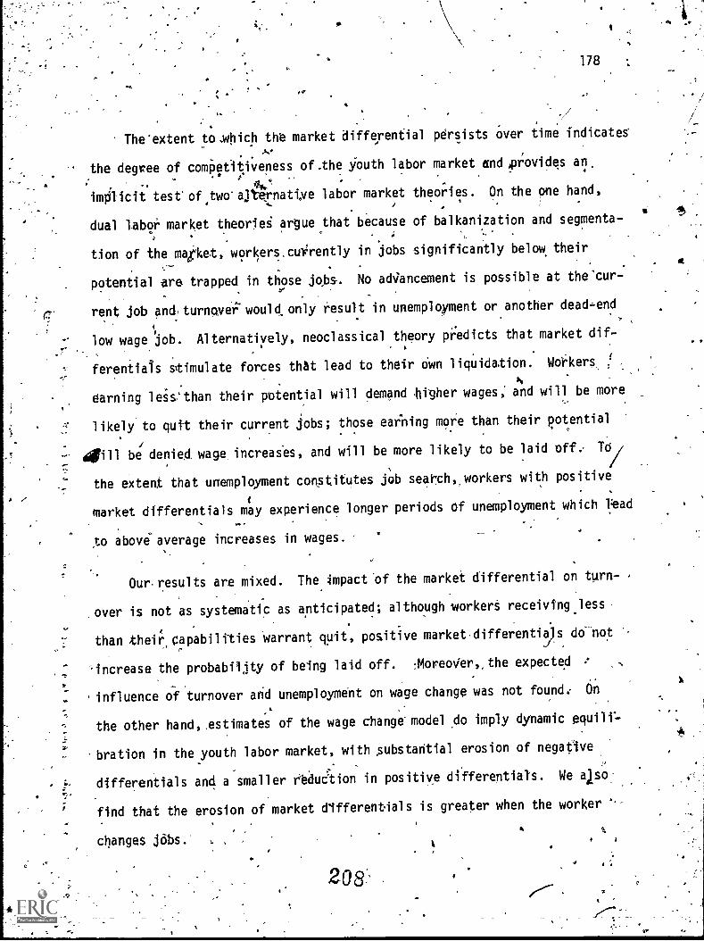
0

The extent to,which the market differential

the degree of competitiveness of.the Youth labor

4

178

persists Over time indicates'

market dnd,provides an,, .. F

. ,,.

v *044,

imOlicit testof two'ajternattve labor market theories. On the one hand,. , .

dual labor market theoriei argue that because of balkanization and segmenta-

tion of the market, workers.cuirently in jobs significantly below their

potential are trapped in those jobs. No advancement is possible at the'cur-

rent job auLturnovetwouldonly result in unemployment or another dead -end

low wage job. Alternatively, neoclassical theory pi:edicts that market dif-.

ferentials sttimulate forces that lead to their Own liquidation. Workers,

earning less'than their potential will demand higher wages; and will be more

likely to quit their current jobs; those earning more than their potential

011 be denied wage, increases, and will be more likely to be laid off.- TO/7

the extent that unemployment constitutes job search, workers with positive

market differentials may experience longer periods of unemployment which lead

to above'average increases in wages.

Our. results are mixed. Theimpact 'of the market differential on turn-

over is not as systematic as anticipated; although workers receivtng.less

than theiricapabilities Warrant quit, positive market.differentia)s do-not

'increase the probabiljty of being laid off. :MoreoVer,,the expected .

.influence of turnover and unemployment on wage change was not found., On

the other hand, estimates of the wage change' model 4o imply dynamic

.bration in the youth labor market, with substahtial erosion of negative

differentials and a smaller reduAion in positive differentials. We als

find that the erosion of market dlfferentials is greater when the worker

changes jobs.

208

*

"Nw

V

179

On the basis of these results, we conclyde that parket forces ficili,

tate the worker's attainment of his human capital or potential iege,although

we are unable to identify the precise channels by which this is achieved.

The asymmetric impact of market differentials indicates a shift in'the wage

I

distribution from year to year, with a deterioration in the relative posi-

--tion of workers initially earning more than the competitive wagealthough

real wages do not actually decline.

t ,r .

4The framework assembled to analyze equilibration in the labor market

_ .

_ n.also permits concurrent analyiigofseveral other interesting topics; of

these, the effects of changing aggtegate economic conditions and race and

sex diScrimination are the most interesting. Here our findings are straight-,.

forward: deteriorating aggregate labor market conditions severely disrupt

the ybuth labor market, increasing unemOloymentrandtdepressing wage growth;. . . . 1..

.

blacks have a great'er incidence of_unemployment and receive substantial wage

discounts, with the discounts dithintshAg over the time period we examine;/

.

.

for both blacks and females, occupational and industrial status are' largelyrgely.

,

responsible for their lower economic standyig.

8.2 Policy Implications

Perhaps the rmost significant fact about the youth labor market from a1.7

policy viewpdint is the severe disruption brought about by declining aggre-

gate economic conditions. The initial jobis 1;1-64e, difficult.to-procure,

young workers are more likely to be pushed out of their Jobs, the duration

of unemployment is extended, and wage growth is depressed. Since the impact

of a downturn falls disproportiodately on youth, macroeconomic policies

designed to increase the overall lei/el of economic activity will be effective

2 0 9

a , .

a

180

in ameliorating many youth labor market protlems. In periods of substantial

overall unemployment, public employment programs (especially for minoritx:..

.

and economically disadvantaged youth) may be useful in providing young

/people with essential work experience.

Dramatic differences, are found in the labor market behavior of males

And females., Even controlling for personal attributes and family background,. ,

males are more likely to continue their education past high school and enter

the labor force later, with lessdiffidulty. A large proportion offemales

are out of the labor force but not enrolled in school, even at.$he youngest

ages, probably reflecting the importance of domestic responsibilities: .

lV

Caning at suctr a critical period in, the life cycle, this break in labor

market experience surely affects their future labor market outcomes adversely.

Because females are not as successful in acquiring actual work experience,

their economic position drops even lower as the aging process continues. The

major *problem, however; 'is not discontinuous work experience: femalesljust

do not obtain high payingjobs consistent with their capabilities. The

:loss in wages resultingfrom discontinuous work' experience is secondary to .

the component of male-female wage differences not explained by variations0

in hOman capital.. In 'many respects, blacks share a similar experience: they

have, lower enrollment rates and higher unemployment rates than whites

(although blacks are somewhat more likely to continue their education con-

trolling for personal attributes and family background). Black wage rates

are'below those of equally, qualified whites, but the aifferential had dimi-

nished somewhat-by the early 1970's. These facts call for continued efforts

.to redude market' discrimination and broaden the range of work opportunities

available to minorities.

21:0

4

bJ 1.

//Hunan capital investments (especially formal dducation, work experience,

and training) have a substantial pOsitive impact on the'earnings of youth,

increasing both the probability of employment and the wage rate. Various

`'programs have been suggested to encourage this investment, including3 . .

"study programs and tuition subsidies for post- secondary, training. .The '

school to work transition of noncollege youth can perhaps be improved by

access to programs of this nature.

In a static setting, many young workers are in jobs belowtheir cap=

abgWes- They are not permanently trapped in these jobs The path upward,

h6wever, is circuitous and usually involves a job and/or occupational change.

Thus, much of the job chagting activity of youth functions to improve the

worker-job match. 'Improved.information and counseling services could, help.

accomplish this desirable mating of4iorkers and jobs.

We would like to know,,much mod about the,youth4labOr market. TO most

serious deficiency of the study is our limited investigation of job turnover

and unemployment. We restricted the sample to job changers; that is, per-

sons employed in'consetutive survey years. This group'appears to enjoy a

relatively smooth adjustment to the market, with a very low incidence of

unemployment and wages moving quickly upward to liquidate noncompensatingwe I.

differentials. Greater difficulties are encountered by those who quit or-

`are laid off but are not employed at the subsequent survey. Since we did

not analyzktheir eventual adjustment Wthe labormarket, it:is difficult.

to draw ciicluiionsabout the efficiency of the market mechanism. Future

work should.include.both job leavers and new labovPmarket entrants in the

analysis.

211 .

0

- °

Another important gap in the study is our 'inability to measure attri-.

butes,.. especially training opportunities, associatecj With the current job.

Va riations in these training opportunities may well account,for part of

the wage growth observed between surveys.

-

Finally, it must be emphasized that the Youth labor market we examine

was that of the 1966 to 1971 period. Since that time, the demographic,

picture has begun to change drastically, with steady declines in the number

Of young people preparing to move into the la or market. In addition

social and legal pressure mit4gating against cial'and seXua discrimina

tion has continued. These factors may well havk resulted in substantial

structural changes in the youth labor market in ?'cent years.

212

4

"-

4-

References

e

Arvil Adams and Garth Mangum, ThdLingeringCrises of Youth Unemployment,

Kalamazoo: .W. E. Upjohn Institute for Employment Research (1977',

typescript).

A. A. Alchian, "Information Costs, Pricing and Resource,OnemplOyment,"

in Microeconomic Foundations Of Employment and Inflation Theory,

E. T715.0WITC710.15111970): .27-52; '

Pauf-Andrisani, "Am Empirical Analysis of t he Dual LaborMarket Thedry,",Columbus:

Center/for Human Resource Reseallph (1973).

Paul.Andrisani and Gilbert Nestel, "Internal-External Control and Labor

Market Experience," in PrellRetihment Years Volume IV (1974).

csJoseph R. Antos, and Sherwin.Rosen. ' iscriminAtion in the Market for Public' School

Teachers," Journal of Econometri (1975): 123-150.

Yonathan Bard, "Nonlinear Parameter Estimation and Programming," IBM (December 1967)

John aon and Wesley Mellow, "JOb.SearCh Intensity4 Theory and Evidence, "`

BLS liorking Paper ;1978). ;

Ann P. Bartel and George J. Borjas,Middle-Age Job Mobility: Its Determinantsand Consequences," NBER Working.:Paper (January 1977).

-'

York:: Columbia University Press (1975).

Partitipation in Labor Organizations," Monthly -Labor

Gary Beckdr, Humin.Capital, New

Virginia'A. Ber9quist, "WMans5Revieg (October 1974): 3-9

Alan Blinder, "Wage Discrimjnation: ?educed Form and Structural Estimates,"Journal of Human Resources, (Fall:1973): 436-455.

Barry A. Bluestone, "The Personal-Eari ings,Distribution: Individual and Institu-tional Determinants,",unpubl;ished Ph. D. Dissertation,-University of Michigan(1974): ,

/

arles Brown,"Equallzing Differences:in the Labor Market:" BLS Working Paper (1.977)\

John F.'Burton, Jr.. and John Parker, !Intent-industry Variations in Voluntary LaborMobility," Industrial and Labor RelatiOns'Review (January 1969): 199-216.

- ! ;

'Glen Cain, "The Challenges of Segmented Labor Market Theories to Orthodox TheoA Surveys't, Journal of Economft Literature (December 106)i- 1215-1257.

Center for Human Resodrce Research, The National LonOtudinaLSurveys'Handbook, Columbus: Ohio State University (1973).

.Martin David, "The Dynamics of Family Labor Supply Decisions: Quittinv4and Relocating as Family,Unit Decisions,"in James N. Morgan, ed.,Five Thousand American Families - Patterns' of economic Progress,'

Vo . II, Ann Arbor: Survey Research Center (1974).

Peter B-Doeringer and Michael J.. Piore, Internal Labor Markets and ManpowerA al sis, Lexington, Mass.:' Health IT71).-

(

T. Domencich and'D. McFadden, Urban Travel Demand: A Behavioral Anaysis-,Armsterdam: North Holland t1975).

Greg Duncan and FraA Stafford, "Pace of WOrk, Unions and Earnings in Blue CollarJobs;".Uhiversity of Michigan, unpublish9d=(March 1977).

Otis Dudley Dundan, David L. Featherman, and Beverly Duncan, SOcideconomiC Back-ground and Achievement, NeW York: Seminar Press (1972):

R. G. Ehrenberg andiR. L. Oaxaca, "Unemployment Insurance,' Duration of'Unemploy-

.ment and Subsequent Wage Gain," American Economic Review (December 1976):%.

754-66.,

Alan A. Fisher, "The Problem of Teenage Unemploymerft,t unpublished, Ph. D. Disserta-

iion) University of California, Berkeley (1973). :

Robert J. Flanagan, "Labor Forcb\Experience, Job Turnover and Racial WageDifferentials," Review of Economics and Statistics (November 1974): 521-29.

Robert's). Flanagn, "Discrimination Theory, Labor Turnover and Racial UnemploymentDifferentials," University of Chicago, Mimeo (1975).

Hugh Folk, "The Probigm'of YoUth Unemplpyme " in The Transiticefrom School to )

Work, Industrial RelatiOns.Sectioh, esearc ,Report 111, Princeton:

Wiiicetonotiniversity Presi' (1968): 76-107.

Richard,B. Freeman, "Chang'esin the Labor Market for Black Americans," Brookings,

.Papers 411 Economic Activity (1973): 67-1 2'.

-

Richard Freeman, ?Teenage Unemployment: in ReallocatingsEducdtional

Resources Help?"'in The Teenage Unemployment Problem: What arettOptiont, Conuresional Yudge! Ofr!,..e Repara&tober 1970! 41-47.

= R. J. Gordon, "The Welfare Cotts of Higher Unemployment," Brookings Papers on

. Economic'Activity (1973):, 133-95.

a 214

185

John Grasso, "Djmensiona of Youth. Unemployment," Chapter 5 in CareerThreshold:.. olume VI (1977).

GrIliches,,"Estimating the Returns to Schooling: Some Ecdnometric Problems,"Econometrica(January 1977): 1 -22.

'Zvi Griliches, ':Wages of yery Young Men," Journal of Political Economy "(August 1976,Parr 2): 569-86.

Zvi Gri3iches and William M. Mason, "Education, Inpome and fibility," Journal ofPolitical Economy (May/June 1972): S74-S103(

Robert Hall, '"Turnover in the Labor Force," Brookings Papers on Economic Activity(1972): 709-56. . /

Giora Hanoch, "An Economic Analysis of Earnings and Schooling," Journal of HumanResources (Summer 1967): .310 -29.

Robert M. Hauser, "Disaggregating a Social-Psychological Model of Educa-

ttonal Attainment," In Structural Equation Models in the Social

Scjences, A.S. Goldberger and 0.D. Duncan -(eds.), New York:, Seminar

Press (1973? 255-284.

James Hetkman,' "Shadow Prices, Market Wages and Labor Supply," Econometrica

(July-1974): 679-694.

'Ns

James Heckman and Robert Willis, "A Beta-Logistic Model ?Or the Analysis of

Sequential Labor Force Participation by Married "Womcn,". Jourtlal of

Political Economy (February 1977): 27-58.

Janice N. Hedges, "Youth Unemployment in 1974-75 Recession," Monthlyjabor Review-

(January 1976): 49 -56.

Christopher Jencks, et al., Inequality: A Reassessmer4 of the Effect of Family

and Schooling in AmerAa, New York: Basic Books (1972).-

Hilda Kahne with Andrew I. Kohen, "Economic Perspectives on the Roles of Women

in the American Economy," Journal of'Economic Literature (December-1975):

1249-1292.

Edward Kalachek, The Youth Labor Market,'Ann Arbor: Institute of "-Labor and

Industrial Relations, University of Michigan and Wayne State University (1969).

. /

Edward Kalachek and Frederic Raines, "The Structure of Wage Differences Among

Mature Male Workers," Journal 'of.Human Rr,..ourref: (r711 1970: 484-506.

fo

Andrew F. Kohen, "Women and the EconOmy: A Bibliography and a Review of the

Literature on Se;i Differentiation in the Labor Market," Columbus: Centel

for Human Resource Resedrth (1975).

2.15

O

186

/*-

Andrew I. Kohen and Paul Andrisani, "Labor Market Experience of High

School Graduates and Dropouts," Chapter 2 in Career Threshold('

Volume IV (1973)) y

Andrew I.- Kohen and Roger D. Roderick, "The Effects of Race and Sex Discriminationon Early-Career Earnings,", Columbus: Center for Huhlan TNesouice Research (1975)

Andrew I. Kohen and Patricia Shields, 4leterminants and Consequences of, Service in the Armed Forces During the Vietnam Era," Chapter 6 in

Career ThresholCs Volume VI,(1977). ,

Edward Lazear, "Age,. xperience and Wage Growth,",American Economic Review(September 1976): 548-58.

Edward Lazear, "Family, Background and Optimal Schooling Decisions," NBER WorkingPaper (Julb 1976).

Edward L zear, "Schooling as-a Wage Depressant," Journal of Human Resourcesi

1

.

.- ..--,--, , (Sp ing 1977): 164-76. . ., ,

. .

Duane E. Leigh, "An Analysis of the Determinants of Occupational Upgrading,"Institute for Research on,Poverty, Uniyersity of Wisconsin - Madison(September,1975).

Robert I. Lerman, "Some Determinants of Youth School Activity," Journal of HumanResources (Summer 1972): 66-383.

Lee Lillard, "Inequaltty: Earnings vs Human Wealth," American Economic Review(March 1977).

S. A. Lippman and J. J. McCall, "ThefEconomics of Job Search: A Survey,"Economic Inquta (June 1976): 313-68.

G,A. Maddala and Lung-Fei Let, "Recursive Models with QualitatiVe-Endogenous( Variables," Annals of Economic and Social Measurement (Fall 1976): 525-546:

Charles D. Mallar, "Estimating a Simultaneous Probability Model: The School'

and Labor Force Decisions of Youths," Proceedings of the Business and EconomicStatistics Section, American Statistical Association (1976): 448-00.

Ray Marshall, "TheEconomicS"of Racial Discrimination: A Survey," Journal ofEconomic Literature (September 1974): 849-871.

Stanley H. Masters, "The Effect of Family Income on Children's Education: Some

Findings on Inequality of Opportunity," Journal of Human Resources (Spring 1969).

158-175.

J. P. Mattila, "Job Quitting and Frictional Unemployment," American EconomicReview .(March 1974): 235-39.

J. J. McCall, "Economics of InforMation and Job Search," Quarterly Journal ofEconomics (February 1970): 113-26,

Raymond,R. Mckay, Wa e Differentials b Sex Amon Em lo ed Youths, unpublished P . D.

d1s4artation, o tate Un vers fy

187

Wesley Mellow, , "Market Differentials and Labor Force Behavior," unpublished Ph. D.'dissertation, Washington University (1975).

Wesley Mellow, "A Multinomial Logic Lodel of Labor Turnover," BLS Working Paper (1977).,

Wesley Mellow., "Search Costs and -the Duration of Unemployment," Economic

Inquiry (forthcoming 1978) (a)."

Wesley Mellow, "Equilibration in the Labor Market," Southern Economic Journal

(forthcoming, July 1978) (b).

Jacob Mincer, Schooling, Experience and Earnings, New York:

Jacob Mincer, "On the'Job Training: Costi, Rdturns, and SomeJournal of Political Economy (October 1962, Supplement):

Gbiumbia (1974).

Implications,"50-79.

Jacob Mincer and Solomon Polachek, "Family Investments in Human Capital: Earningsof Women," Journal of Political Economy'March/April 1974, SUpplement): 'S76-S108.

4,

Forrest D. Nelson, "On a General Computer Algorithm _for the Analysis of Modelswith Limited Dependent Variables, Annals.of Economic and Social Measurement(Fall 1976): 493-510.

Marc Nerlove and S. J. Press, "Univariate and Multivariate Log-Linear and LogistiModels,"-Santa Monica: The Rand Corporation (1973), R-1306-EDA/NIH,

Ronald Oaxaca, "Male-Female Wage Differentials in Urban Labor_ Markets," International.Economic Review (October 1973): 693-709.

Michael D. Ornstein, Entry into the American Labor Force, New York: Academic Press(1970.4

Herbert S. arne&sand Andrew I. Kohen, "Labor Market xperience of NoncollegeYouth: A Longitudinal Analysis," in From School to Work: Improving the '

'Transition, Washington: National Commission for Manpower Policy (1976): 57-8

Herbert S. Parnes and Andrew I. Kohen,-"Occupational Information and Labor Market.Status: The Case of Young Men," Journal of Human Resources' (Winter 1975): 45-55.

Donald Parsons, "The Cat of School Time,. Forgone Earnings and Human Capitalformation,". Journal bf-Politital Economy (March 1974):. 25146.

Donald 0. Parsons, "IntergeneratiOnal Weal. of Male Youth, !' Quarterly Journal of

Donald O. Parsons, "Specific Human CapitalRates," Journal of Political Econ:n

th TranifersaWd the Educational becisionsEconomiest(1974):e 603-617-

An Application to Quit:Rates end Layoff.(U -( tuber ,1972): 1120-1143.,

Donald O. Parsons, "Mode cis of Labor Market Turnover: A Theoretical andEmpirical Survey," in Resoarch in Labor Economics, Ronald G. Ehrenberg'(e0.), Greenwich, Connecticut: JAL eress7M77177

217

.

JOhn H. Pencavel, An Analysis of the Quit Rate in American Manufacturing Industry,

.Princeton,(1970), $

188

#,

Perry, "Unemployment Flows in the'U.S. Labor Market," Brookings Paperson,Economic Activity (1972): 245-78.'

F. Ragan, Jr., "Minimum Wages and the Youth Labor Market," Review ofc nodtics.,,and Statistics (NO 1977): .129136.. - r

4 \,

Sherwin Rosen, "t rman Capital: A Survey of.Empirical Research,'' in Research ina a

Labor Economics, leonaldPG.'Ehrenberg (ed.), Greenwfch, Connecticut; JAI

Press (1977).,

Sherwin Rosen': "Learning and Experience in the Labor Market," Journal of Human

Resources (Summer 1972): 326-342.,

,Peter Schmidt and Robert Strauss, "The Effect of Unions on Earnings and.Earnings

on Unions: A Mixed Logit Approach," International Economic Review(February 1976):

0,

James P. Smith and Finis R. Welch, "Black-White Earnings,and Employment:

1960-1970," Technical' Analysis Paper No. 3 ASPER (June )975).'

Michael Spence, "Job Market Signalling,I! Quarterly" Journal of Economics

(,August 1973);

Stanley P. Stephenson, Jr.; "The Economics of YO;ith Job Search Behavior,"

Review of Economics and Statistics (February 1976): 104-11., 't

C..

..

Stanley:P. Stephenson, Jr., "The Transition from School to Work of

Young Men," preserved at, the American Economic Association Meeting, . .

December 1977.

1

0. ,

Betweeniftne Stevenson,7he Relationship Early'Work Experience and

Future Employability,"Chapter 6 in Adams:and Mangum (1977)-%.

+

'Vladimir Stoikov and Robert L. Raimoni,"Detirminants of the Differences in Quit

Rates Among Industries," American Economic Review (December 1968): 283 -98.

Paul Taubman, Sources of Inequality in Earnings, Amsterdam: No ,Holland (1975);

Richard Thaler and-Sherwin Rosen, "The Value of Saving a Life: 'Evidence from the

Labor Market," in Household Production and' sumption, Nestor Terleckyj (ed.):

New York: NBER (1975): 265-297.

ii. S. Department of Labor, Handbook of Labor Statistics 1976, Bulletin 1905,

U. S. Government Printing Office (1976).

, .

0

21.8

r

4

189

U. S. Department of Labor, BLS Handboorof Methods, Bulletin 1910; U. S. Government'Printing Office (1976).

U. S. DepartMent of Labor, Career Thresholds, Manpower Research Monograph No. 16,Vols. 1-5, U. S. Government Printing Office (1970-1975).

U. S. Department of Labor, Years for Decision, ManpOwer Research Monograph go. 24,

Vols. 1-3, U. S. Government Printing Office (1970-1975).7

Howard Wachteland Charles Betsey, "Employment at Low Wages," Review of Economicsand Statistics (May 1972): 121-28. .

Michael L. Wachter, "Primary and SecOndary Labor Markets: A Critique of theDual

'Approach," Brookings Papers on Economic Activity (1974): 637-693.

a

Leonard Weiss, "Concentratton(March 1966): 96-117

Leonard Weiss'and Jeffrey G.Interregional Migration:(March 1975): 241-244.

and Labor Earnings," American Economic Review.

r

Williamson, "Bladk Education, Earnings andEven Newer Evidence," American Economic Review

.Randall,D. Weiss, "The Effect of Education on the Tarningsof Blacks and Whites,"lAview of Economics and Statistics (MaS, 1970): 150-159. .

Finis Welch, "Black-White Returns to Schooling," American Economic Review(March 1973): 893-907.

0T