Embed Size (px)
Citation preview

Full-Text Indexing
Session 10
INFM 718N
Web-Enabled Databases

Agenda
• How to do it
• How it works
• The “A” Team

Database
Server-side Programming
Interchange Language
Client-side Programming
Web Browser
Client Hardware
Server Hardware (PC, Unix)
(MySQL)
(PHP)
(HTML, XML)
(JavaScript)
(IE, Firefox)
(PC)
Bus
ines
sru
les
Inte
ract
ion
Des
ign
Inte
rfac
eD
esig
n
• Relational normalization• Structured programming• Software patterns• Object-oriented design• Functional decomposition

Full-Text Indexing in MySQL
• Create a MyISAM table (not InnoDB!)– Include a CHAR, VARCHAR, or TEXT field– Text fields can hold a bit over 10,000 words
• Create a FULLTEXT index– ALTER TABLE x ADD FULLTEXT INDEX y;
• Issue a (ranked) query– SELECT y FROM x WHERE MATCH y AGAINST
(‘cat’);

Other Types of Queries
• Automatic (ranked) vocabulary expansion– SELECT y FROM x WHERE MATCH y AGAINST
(‘cat’ WITH QUERY EXPANSION);
• Boolean (unranked) search– SELECT y FROM x WHERE MATCH y AGAINST
(‘+cat -dog’ IN BOOLEAN MODE);

Query Details
• No more than 254 characters (~40 words)– Longer queries take more time
• Multiple words are implicitly joined by “OR”
• Boolean queries can use (unnested) operators– Words preceded by “+” must occur (AND)– Words preceded by “-” must not occur (AND NOT)

What’s a “Word?”
• Delimited by “white space” or “-”– White-space includes space, tab, newline, …
• Not case sensitive• Exact string match
– No “stemming” (automatic truncation)
• Boolean search has additional options– Truncation (e.g., time*)
– Phrases (e.g., “cats and dogs”)

Unsearchable Words
• Very common words– Those that appear in more than 50% of docs
• Words of 3 or fewer characters– Rarely are topically specific
• Other “stopwords”– able about above according accordingly across
actually after afterwards again against ain't …

Human-Machine Synergy
• Machines are good at:– Doing simple things accurately and quickly– Scaling to larger collections in sublinear time
• People are better at:– Accurately recognizing what they are looking for– Evaluating intangibles such as “quality”
• Both are pretty bad at:– Mapping consistently between words and concepts

Supporting the Search Process
SourceSelection
Search
Query
Selection
Ranked List
Examination
Document
Delivery
Document
QueryFormulation
IR System
Query Reformulation and
Relevance Feedback
SourceReselection
Nominate ChoosePredict

Supporting the Search Process
SourceSelection
Search
Query
Selection
Ranked List
Examination
Document
Delivery
Document
QueryFormulation
IR System
Indexing Index
Acquisition Collection

Taylor’s Model of Question Formation
Q1 Visceral Need
Q2 Conscious Need
Q3 Formalized Need
Q4 Compromised Need (Query)
En
d-u
ser
Sea
rch
Interm
ediated
Search

Search Goal
• Choose the same documents a human would– Without human intervention (less work)– Faster than a human could (less time)– As accurately as possible (less accuracy)
• Humans start with an information need– Machines start with a query
• Humans match documents to information needs– Machines match document & query representations

Search Component Model
Comparison Function
Representation Function
Query Formulation
Human Judgment
Representation Function
Retrieval Status Value
Utility
Query
Information Need Document
Query Representation Document Representation
Que
ry P
roce
ssin
g
Doc
umen
t P
roce
ssin
g

Relevance
• Relevance relates a topic and a document– Duplicates are equally relevant, by definition
– Constant over time and across users
• Pertinence relates a task and a document– Accounts for quality, complexity, language, …
• Utility relates a user and a document– Accounts for prior knowledge
• We seek utility, but relevance is what we get!
Problems With Word Matching
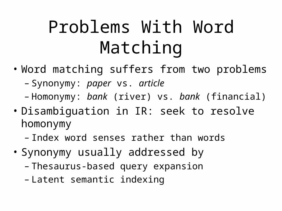
• Word matching suffers from two problems– Synonymy: paper vs. article– Homonymy: bank (river) vs. bank (financial)
• Disambiguation in IR: seek to resolve homonymy– Index word senses rather than words
• Synonymy usually addressed by – Thesaurus-based query expansion– Latent semantic indexing

“Bag of Terms” Representation
• Bag = a “set” that can contain duplicates “The quick brown fox jumped over the lazy dog’s back”
{back, brown, dog, fox, jump, lazy, over, quick, the, the}
• Vector = values recorded in any consistent order {back, brown, dog, fox, jump, lazy, over, quick, the, the}
[1 1 1 1 1 1 1 1 2]
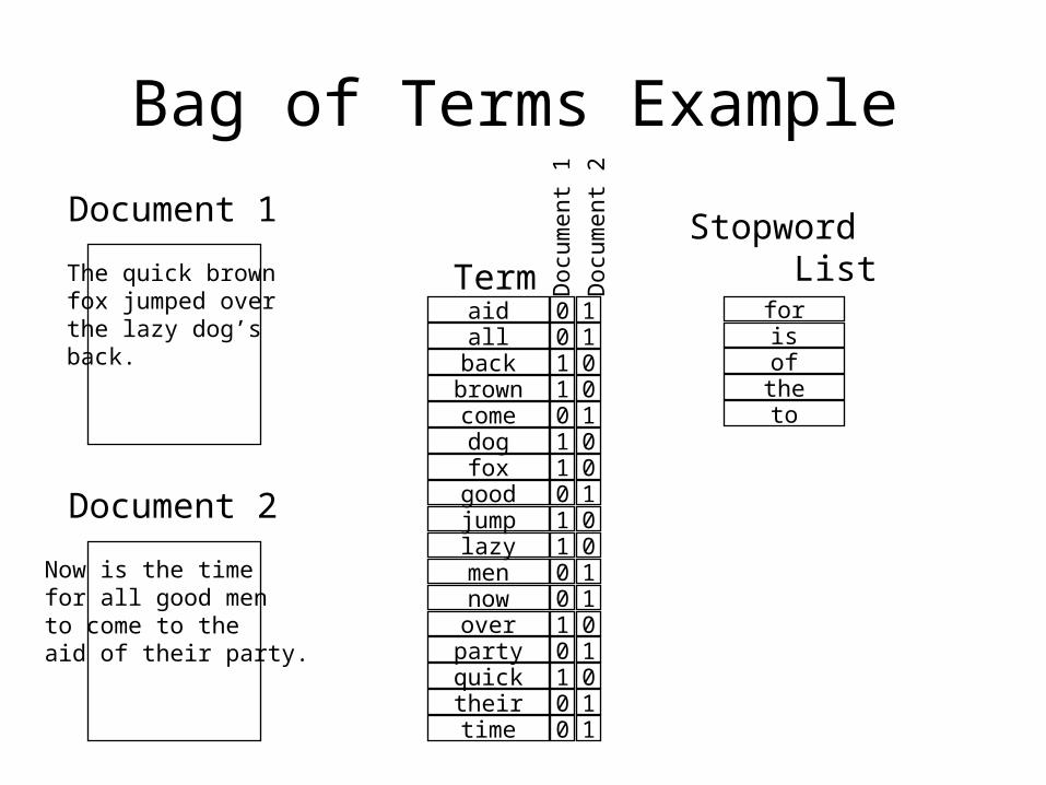
Bag of Terms Example
The quick brown fox jumped over the lazy dog’s back.
Document 1
Document 2
Now is the time for all good men to come to the aid of their party.
the
quick
brown
fox
over
lazy
dog
back
now
is
time
forall
good
men
tocome
jump
aid
of
their
party
00110110110010100
11001001001101011
Term Doc
umen
t 1
Doc
umen
t 2
Stopword List

Boolean IR
• Strong points– Accurate, if you know the right strategies
– Efficient for the computer
• Weaknesses– Often results in too many documents, or none
– Users must learn Boolean logic
– Sometimes finds relationships that don’t exist
– Words can have many meanings
– Choosing the right words is sometimes hard

Proximity Operators
• More precise versions of AND– “NEAR n” allows at most n-1 intervening terms– “WITH” requires terms to be adjacent and in order
• Easy to implement, but less efficient– Store a list of positions for each word in each doc
• Stopwords become very important!
– Perform normal Boolean computations• Treat WITH and NEAR like AND with an extra constraint

Proximity Operator Example
• time AND come– Doc 2
• time (NEAR 2) come– Empty
• quick (NEAR 2) fox– Doc 1
• quick WITH fox– Empty
quick
brown
fox
over
lazy
dog
back
now
time
all
good
men
come
jump
aid
their
party
0 1 (9)
Term1 (13)1 (6)
1 (7)
1 (8)
1 (16)
1 (1)
1 (2)1 (15)1 (4)
0
00
0
00
0
0
0
0
0
0
00
0
0
1 (5)
1 (9)
1 (3)
1 (4)
1 (8)
1 (6)
1 (10)
Doc
1
Doc
2

Advantages of Ranked Retrieval
• Closer to the way people think– Some documents are better than others
• Enriches browsing behavior– Decide how far down the list to go as you read it
• Allows more flexible queries– Long and short queries can produce useful results

Ranked Retrieval Challenges
• “Best first” is easy to say but hard to do!– The best we can hope for is to approximate it
• Will the user understand the process?– It is hard to use a tool that you don’t understand
• Efficiency becomes a concern– Only a problem for long queries, though

Similarity-Based Queries
• Treat the query as if it were a document– Create a query bag-of-words
• Find the similarity of each document– Using the coordination measure, for example
• Rank order the documents by similarity– Most similar to the query first
• Surprisingly, this works pretty well!– Especially for very short queries

Counting Terms
• Terms tell us about documents– If “rabbit” appears a lot, it may be about rabbits
• Documents tell us about terms– “the” is in every document -- not discriminating
• Documents are most likely described well by rare terms that occur in them frequently– Higher “term frequency” is stronger evidence– Low “collection frequency” makes it stronger still
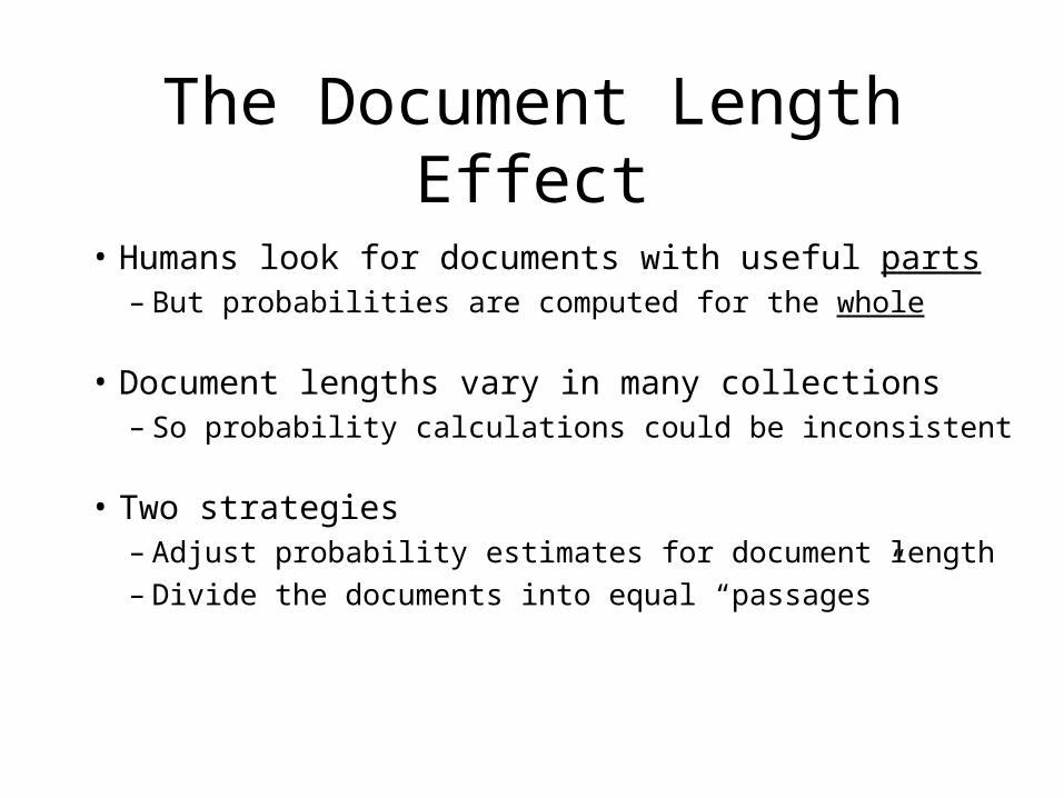
The Document Length Effect
• Humans look for documents with useful parts– But probabilities are computed for the whole
• Document lengths vary in many collections– So probability calculations could be inconsistent
• Two strategies– Adjust probability estimates for document length– Divide the documents into equal “passages”

Incorporating Term Frequency
• High term frequency is evidence of meaning– And high IDF is evidence of term importance
• Recompute the bag-of-words– Compute TF * IDF for every element
Let be the total number of documents
Let of the documents contain term
Let be the number of times term appears in document
Then
N
n N i
i j
wN
n
i j
i j i j
tf
tf log
,
, ,

TF*IDF Example
4
5
6
3
1
3
1
6
5
3
4
3
7
1
nuclear
fallout
siberia
contaminated
interesting
complicated
information
retrieval
2
1 2 3
2
3
2
4
4
0.50
0.63
0.90
0.13
0.60
0.75
1.51
0.38
0.50
2.11
0.13
1.20
1 2 3
0.60
0.38
0.50
4
0.301
0.125
0.125
0.125
0.602
0.301
0.000
0.602
idfi Unweighted query: contaminated retrievalResult: 2, 3, 1, 4
Weighted query: contaminated(3) retrieval(1)Result: 1, 3, 2, 4
IDF-weighted query: contaminated retrievalResult: 2, 3, 1, 4
tf ,i jwi j,

Document Length Normalization
• Long documents have an unfair advantage– They use a lot of terms
• So they get more matches than short documents
– And they use the same words repeatedly• So they have much higher term frequencies
• Normalization seeks to remove these effects– Related somehow to maximum term frequency– But also sensitive to the of number of terms

“Okapi” Term Weights
5.0
5.0log*
5.05.1 ,
,,
j
j
jii
jiji DF
DFN
TFLL
TFw
0.0
0.2
0.4
0.6
0.8
1.0
0 5 10 15 20 25
Raw TF
Oka
pi
TF 0.5
1.0
2.0
4.4
4.6
4.8
5.0
5.2
5.4
5.6
5.8
6.0
0 5 10 15 20 25
Raw DF
IDF Classic
Okapi
LL /
TF component IDF component
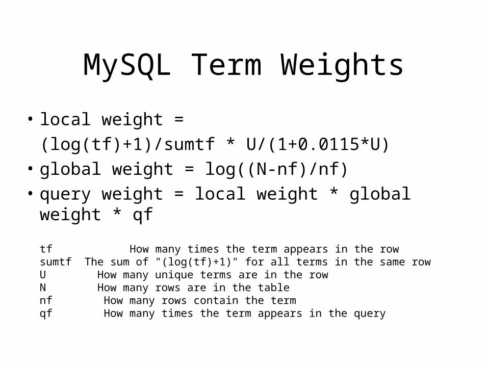
MySQL Term Weights
• local weight =
(log(tf)+1)/sumtf * U/(1+0.0115*U)
• global weight = log((N-nf)/nf)
• query weight = local weight * global weight * qf
tf How many times the term appears in the rowsumtf The sum of "(log(tf)+1)" for all terms in the same rowU How many unique terms are in the rowN How many rows are in the tablenf How many rows contain the termqf How many times the term appears in the query

Summary
• Goal: find documents most similar to the query
• Compute normalized document term weights– Some combination of TF, DF, and Length
• Optionally, get query term weights from the user– Estimate of term importance
• Compute inner product of query and doc vectors– Multiply corresponding elements and then add

The Indexing Process
quick
brown
fox
over
lazy
dog
back
now
time
all
good
men
come
jump
aid
their
party
00110000010010110
01001001001100001
Term Doc
1
Doc
2
00110110110010100
11001001001000001
Doc
3D
oc 4
00010110010010010
01001001000101001
Doc
5D
oc 6
00110010010010010
10001001001111000
Doc
7D
oc 8
A
B
C
FD
GJLMNOPQ
T
AIALBABR
THTI
4, 82, 4, 61, 3, 7
1, 3, 5, 72, 4, 6, 8
3, 53, 5, 7
2, 4, 6, 83
1, 3, 5, 72, 4, 82, 6, 8
1, 3, 5, 7, 86, 81, 3
1, 5, 72, 4, 6
PostingsInverted File

The Finished Product
quick
brown
fox
over
lazy
dog
back
now
time
all
good
men
come
jump
aid
their
party
Term
A
B
C
FD
GJLMNOPQ
T
AIALBABR
THTI
4, 82, 4, 61, 3, 7
1, 3, 5, 72, 4, 6, 8
3, 53, 5, 7
2, 4, 6, 83
1, 3, 5, 72, 4, 82, 6, 8
1, 3, 5, 7, 86, 81, 3
1, 5, 72, 4, 6
PostingsInverted File

How Big Is the Postings File?
• Very compact for Boolean retrieval– About 10% of the size of the documents
• If an aggressive stopword list is used!
• Not much larger for ranked retrieval– Perhaps 20%
• Enormous for proximity operators– Sometimes larger than the documents!

Building an Inverted Index• Simplest solution is a single sorted array
– Fast lookup using binary search– But sorting large files on disk is very slow– And adding one document means starting over
• Tree structures allow easy insertion– But the worst case lookup time is linear
• Balanced trees provide the best of both– Fast lookup and easy insertion– But they require 45% more disk space

How Big is the Inverted Index?
• Typically smaller than the postings file– Depends on number of terms, not documents
• Eventually, most terms will already be indexed– But the postings file will continue to grow
• Postings dominate asymptotic space complexity– Linear in the number of documents

Summary
• Slow indexing yields fast query processing– Key fact: most terms don’t appear in most documents
• We use extra disk space to save query time– Index space is in addition to document space– Time and space complexity must be balanced
• Disk block reads are the critical resource– This makes index compression a big win