FULL WAVEFORM ACTIVE HYPERSPECTRAL LIDAR

FULL WAVEFORM ACTIVE HYPERSPECTRAL LIDAR

T. Hakalaa,*, J. Suomalainena, S. Kaasalainena

a Department of Photogrammetry and Remote Sensing, Finnish Geodetic Institute, Geodeetinrinne 2, Masala, 02431,

Finland – (teemu.hakala, juha.suomalainen, sanna.kaasalainen)@fgi.fi

KEY WORDS: Full waveform, Hyperspectral, LiDAR, Supercontinuum, Reflectance, Spectral indices

ABSTRACT:

We have developed a prototype full waveform hyperspectral LiDAR and investigated its potential for remote sensing applications.

Traditionally hyperspectral remote sensing is based on passive measurement of sunlit targets. These methods are sensitive to errors in

illumination conditions and lack the range information. Our prototype can measure both the range and the spectral information from

a single laser pulse. At this stage, the instrument is optimized for short range terrestrial applications. An active hyperspectral LiDAR

opens up new possibilities for LiDAR data analysis. The lack of spectral information in traditional monochrome LiDARs rules out

many of the classification techniques available for processing of hyperspectral data. Similarly, passive hyperspectral data does not

allow extensive use of the classifications based on 3D shape parameters. With both hyperspectral and range data available in a single

dataset, the best of the techniques can be applied to form more reliable classification results. The data also allows the mapping of

spectral indices in 3D. As an example a Norway spruce is measured and spatial distribution of several spectral indices is illustrated.

1. INTRODUCTION

Supercontinuum laser sources produce directional broadband

laser pulses by making use of cascaded nonlinear optical

interactions in a nonlinear optical fiber (see Dudley et al., 2006

for a review). The commercial availability of supercontinuum

laser technology has lead into a number of applications in the

recent years, such as those in biomedical optics (e.g., Kudlinski

et al., 2010). Combined with a hyperspectral time-of-flight

sensor, the supercontinuum laser sources can be used for

simultaneous measurement of distance and reflectance

spectrum, which has been the basis for our recent efforts in

development of the hyperspectral LiDAR.

Simultaneous topographic and spectral remote sensing has thus

far been based on passive imaging spectroscopy, fused with

laser scanner point clouds (Jones et al., 2010; Puttonen et al.,

2011; Thomas et al., 2009). Simultaneous geometric and

spectral information can also be retrieved by the means of a

novel approach for photogrammetric point cloud creation from

automatic multispectral image matching (Honkavaara et al.,

2012). Active hyperspectral imaging applications acquire a

spectral signature for every pixel in the image captured by an

imaging detector, but they do not produce range information

(Johnson et al., 1999; Nischan et al., 2003). Range information

is included in multi-wavelength laser scanners that use separate

monochromatic lasers as light sources for each wavelength

(Pfennigbauer and Ullrich, 2011). For these, the wavelength

channels are determined by the light sources.

The hyperspectral scanning LiDAR combines active

hyperspectral imaging and laser scanning with the same

instrument, with no registration problems between data sets.

The hyperspectral LiDAR produces a point cloud and

hyperspectral reflectance: (x,y,z,R(λ)), where R(λ) is the

backscattered reflectance R as a function of the wavelength λ.

The information content of the new type of data is vast and

creates new prospects for improving automatic data processing

and target characterization for laser scanning (LiDAR) data.

We present the design of a full waveform hyperspectral LiDAR

and its first demonstrations in the remote sensing of vegetation.

The concept was first studied with a scanning active

hyperspectral measurement system (Suomalainen et al., 2011),

where the active hyperspectral intensity data was fused with

simultaneous terrestrial laser scanner measurement. This lead to

the development of the scanning LiDAR instrument presented

in this paper (see also Hakala et al., 2012), and enabled us to

study the usage of hyperspectral 3D point clouds in target

classification (Puttonen et al., 2010). To our knowledge, this is

the first full waveform hyperspectral LiDAR producing spectral

3D point clouds and exploiting the supercontinuum laser

technology, and one of the first environmental applications of

supercontinuum lasers.

2. FULL WAVEFORM ACTIVE HYPERSPECTRAL

LIDAR

2.1 The Instrument

We have assembled an optical setup (Fig. 1) for measuring the

time-of-flight and return intensity of a hyperspectral laser pulse.

The supercontinuum laser (NKT Photonics, SuperK) produces 1

ns pulses at repetition rate of 24 kHz and average power of 100

mW. The broadband output laser is collimated using a

refracting collimator (Thorlabs, CFC-5-A). The collimated

beam passes through a beam sampler, which takes a part of the

beam for triggering the time-of-flight measurement. An off-axis

parabolic mirror (50.8 mm diameter, 152.4 mm effective focal

length and 90° off-axis angle) is used as the primary collecting

optic.

The off-axis parabolic mirror is focused to a spectrograph

(Specim, ImSpector V10). A 16-element avalanche photo diode

(APD) array module (Pacific Silicon Sensor) is used to convert

the spectrally separated light to analog voltages. The APD

module has built-in transimpedance amplifiers (Analog

Devices, AD8015) with a bandwidth of 240 MHz producing an

unambiguous resolution of approximately 4 ns. 12-bit analog to

International Archives of the Photogrammetry, Remote Sensing and Spatial Information Sciences, Volume XXXIX-B7, 2012 XXII ISPRS Congress, 25 August – 01 September 2012, Melbourne, Australia

459

digital converters (SP Devices, ADQ412), with 1 GHz sampling

rate, are used to digitize 8 of the 16 available spectral channels.

An average of 10 pulses is saved to improve signal to noise

ratio and to reduce the amount of data.

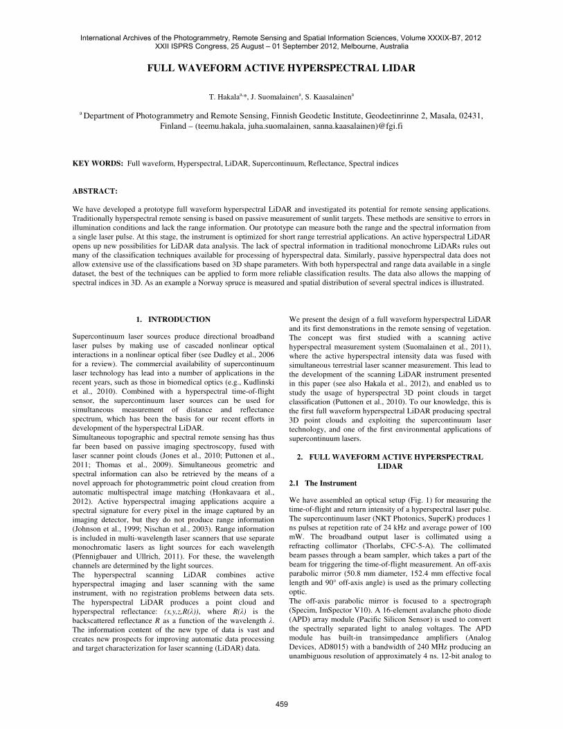
Fig.1. The optical setup: A laser pulse (A) is collimated and

sent to a 2D scanner setup (B). An off-axis parabolic

mirror (C) is used as a primary light collecting optic.

A spectrograph (D) disperses the colors of the return

and trigger (E) pulses to an APD array, which

converts the light to analog voltage waveforms.

The scanning geometry is defined by the two rotators (Newport

URS75BCC and URS100BCC) with an absolute accuracy of

±0.0115°. The rotators are attached to each other, with one

performing the azimuth rotation and the other sweeping the

laser over the target area in vertical passes. Due to uncertainty

in timing, the accuracy of the elevation angles is 0.1°.

2.2 Calibration and Data Processing

A monochromator (Oriel, Cornerstone 74125) was used to

calibrate the spectral responses of the APD elements. The

current configuration produces spectral Full Width at Half

Maximum (FWHM) of about 19 nm for each element and

spectral range of 470-990 nm. However, the sensitivity of the

APD array and the laser intensity below 550 nm are low, and

therefore the first channel is selected to be at 542 nm followed

by 606, 672, 707, 740, 775, 878 and 981 nm.

The transmitted pulse energy of the SuperK laser source may

vary slightly. To take this into account, an average waveform of

all spectral channels is calculated and a Gaussian peak function

is fitted to the trigger part of the waveform and the waveforms

are normalized with the transmit pulse intensity. Similarly, the

return echo positions are detected from a mean waveform,

averaged over all spectral channels. Once the return echo

positions and widths are determined from the mean waveform,

the hyperspectral intensities are extracted by fitting Gaussian

peak heights to the spectral waveforms (Fig. 2).

Fig. 2. Result waveforms for each channel after post processing.

Gaussian peaks are fitted to each of the measured

echoes. The first echo is produced by target spruce

and the second by black cotton background canvas.

The intensity is converted into reflectance by applying the

distance and spectral calibration. During the calibration

measurements, waveforms are collected using a 99% Spectralon

as a reference target at various distances. The echo intensities

are normalized with the intensity of the Spectralon echo at the

same distance, producing “backscattered reflectance”. As the

backscattered reflectance spectra are combined with the

corresponding time-of-flight and concurrent scanner

orientation, a hyperspectral point cloud (x, y, z, R(λ)) is

produced.

The accuracy of the measurement and the Gaussian fitting was

tested by acquiring waveforms of 100 pulses reflected from a

Spectralon panel at a 6-meter distance. The distance and the

backscattered reflectance spectrum were retrieved individually

for each pulse. The precision of ranging (standard deviation)

was found to be 11.5 mm. The precision of backscattered

reflectance of a single waveform was found to be better than 2%

for spectral channels within the range of 600–800 nm and better

than 5.5% for all channels. The quality of the fit is affected by

the return pulse intensity, and thus lower precision is expected

for targets that are darker or further away from instrument.

Higher precision can be reached by averaging over a number of

measurement points. For both range and reflectance, the

absolute accuracy is expected to be lower than the precision due

to uncertainty in calibration.

The instrument does not have a strictly defined maximum range

of measurement, as the performance of the waveform echo

detection decreases slowly with the fading echo intensity. The

current configuration is focused to approximately 12-meter

distance. Measurements have shown that high quality point

clouds can be measured from targets within 10-meter range and

bright targets can be detected even from over 20 meters.

2.3 Results and Discussion

A Norway spruce (Picea abies) (Fig. 3) was measured in

laboratory using the full waveform hyperspectral LiDAR. The

bottom branches of the 2-meter spruce had suffered from lack of

light and were in various stages of drying and dying, while the

top branches had healthy new growth. In addition to the LiDAR

measurement, reference spectra were acquired using a passive

spectrometer (Avantes, AvaSpec 3648) and a quartz-tungsten-

halogen light source.


460

Fig. 3. The Norway spruce.

500 600 700 800 900 10000

0.05

0.1

0.15

0.2

0.25

0.3

TR

EE

TR

UN

K

Spectrometer

LiDAR

TR

EE

TO

P

Spectrometer

LiDAR

Wavelength / nm

Backscattere

d R

eflecta

nce

Fig. 4. Passive spectrometer measurement (solid line) and

hyperspectral LiDAR (dashed line) of same areas of

the tree are shown.

Spectra of the passive spectrometer and LiDAR measurements

of selected regions of interest are presented in Fig. 4. A clear

distinction between the tree trunk and the top can be observed

in the shape of the spectra. The LiDAR and passive

spectrometer spectral shapes are clearly similar. In case of the

tree top, the LiDAR observes less light than the passive

measurement in near-infrared. This difference is caused by

multiple scattering in a medium with a low optical density and a

high single scattering albedo. In an active LiDAR measurement,

only a small spot on the target is illuminated and observed. A

significant part of the pulse energy is lost outside the sensor

field of view, if multiple scattering plays a major role in

reflectance and the scattering mean free path is long in the

medium. This is not experienced in passive measurement as the

same amount of light is scattered both in and out of the sensor

field of view. The backscattered reflectance from Spectralon is

not significantly affected by this effect, as Spectralon has a high

single scattering albedo but only a short mean free path. As the

LiDAR backscattered reflectance is calibrated with that of the

Spectralon panel, the backscattered reflectance values are

decreased for bright and low optical density targets such as

needles.

The backscattered reflectance values produced by the LiDAR

do not strictly follow the definition of reflectance factor for

three reasons: First, due to hot spot effect (Hapke, 1993), the

99% Spectralon is not a Lambertian surface in backscattering

direction causing systematic error in the reflectance values.

Second, the illuminated surface area of the target is not constant

(as in the definition of reflectance factor) and this results in

uncertainty in the returned intensity. Third, part of the

transmitted light is lost outside the sensor field of view due to

multiple scattering, as described above. Despite these

limitations, the backscattered reflectance is a practical quantity

providing intensity readings independent of measurement

distance. For most applications, the backscattered reflectance

spectra can be exploited similarly to traditional reflectance

factors (e.g., in the computation and comparison of spectral

indices), but caution should be used when accurate absolute

values are needed.

Different vegetation indices can be obtained from the measured

dataset. For this study we selected Normalized Difference

Vegetation Index (NDVI) (Tucker, 1979), water concentration

index (Penuelas et al., 1993) and Modified Chlorophyll

Absorption Ratio Index (MCARI1) (Haboudane et al., 2004). In

Fig. 5, these indices have been applied to the measured dataset

of the spruce.

Fig. 5. Different spectral indices are calculated for 5 cm voxels

and the full point cloud is colored according to the

result.


461

3. CONCLUSION

We present the first prototype of a full waveform hyperspectral

terrestrial laser scanner and its first applications in the remote

sensing of vegetation. The instrument provides a novel

approach for one shot spectral imaging and laser scanning by

producing hyperspectral 3D point clouds. The spectra can be

used in, e.g., visualization and automated classification of the

point cloud and calculation of spectral indices for extraction of

target physical properties. The new type of data opens up new

possibilities for more efficient and automatic retrieval of

distinctive target properties, leading to improved monitoring

tools for remote sensing applications, e.g., 3D-distribution of

chlorophyll or water concentration in vegetation. At this stage

the instrument is optimized for short range terrestrial

applications, but we believe that, as technology matures,

hyperspectral laser scanners with extended distance and spectral

range will also become available from commercial

manufacturers.

3.1 References

Dudley JM, Genty G and Coen S (2006) Supercontinuum

generation in photonic crystal fiber. Reviews of Modern Physics

78(4): 1135.

Haboudane D, Miller JR, Pattey E, Zarco-Tejada PJ and

Strachan IB (2004) Hyperspectral vegetation indices and novel

algorithms for predicting green LAI of crop canopies: Modeling

and validation in the context of precision agriculture. Remote

Sensing of Environment 90(3): 337-352.

Hakala T, Suomalainen J, Kaasalainen S and Chen Y (2012)

Full Waveform Hyperspectral LiDAR for Terrestrial Laser

Scanning. Submitted to Optics Express.

Hapke B (1993) Theory of Reflectance and Emittance

Spectroscopy. Cambridge, UK: Cambridge University Press.

Honkavaara E, Markelin L, Rosnell T and Nurminen K (2012)

Influence of solar elevation in radiometric and geometric

performance of multispectral photogrammetry. ISPRS Journal

of Photogrammetry and Remote Sensing 67: 13-26.

Johnson B, Joseph R, Nischan M, Newbury A, Kerekes J,

Barclay H, et al. (1999) A Compact, Active Hyperspectral

Imaging System for the Detection of Concealed Targets. :

International Society for Optical Engineering (SPIE).

Jones TG, Coops NC and Sharma T (2010) Assessing the utility

of airborne hyperspectral and LiDAR data for species

distribution mapping in the coastal Pacific Northwest, Canada.

Remote Sensing of Environment 114(12): 2841-2852.

Kudlinski A, Lelek M, Barviau B, Audry L and Mussot A

(2010) Efficient blue conversion from a 1064 nm microchip

laser in long photonic crystal fiber tapers for fluorescence

microscopy. Optics Express 18(16): 16640-16645.

Nischan M, Joseph R, Libby J and Kerekes J (2003) Active

spectral imaging. Lincoln Laboratory Journal 14: 131-144.

Penuelas J, Filella I, Biel C, Serrano L and Save R (1993) The

reflectance at the 950–970 nm region as an indicator of plant

water status. International Journal of Remote Sensing 14(10):

1887-1905.

Pfennigbauer M and Ullrich A (2011) Multi-Wavelength

Airborne Laser Scanning. : ILMF 2011.

Puttonen E, Jaakkola A, Litkey P and Hyyppä J (2011) Tree

Classification with Fused Mobile Laser Scanning and

Hyperspectral Data. Sensors 11(5): 5158-5182.

Puttonen E, Suomalainen J, Hakala T, Räikkönen E, Kaartinen

H, Kaasalainen S, et al. (2010) Tree species classification from

fused active hyperspectral reflectance and LIDAR

measurements. Forest Ecology and Management 260(10):

1843-1852.

Suomalainen J, Hakala T, Kaartinen H, Räikkönen E and

Kaasalainen S (2011) Demonstration of a virtual active

hyperspectral LiDAR in automated point cloud classification.

ISPRS Journal of Photogrammetry and Remote Sensing.

Thomas V, McCaughey J, Treitz P, Finch D, Noland T and

Rich L (2009) Spatial modelling of photosynthesis for a boreal

mixedwood forest by integrating micrometeorological, lidar and

hyperspectral remote sensing data. Agricultural and Forest

Meteorology 149(3-4): 639-654.

Tucker CJ (1979) Red and photographic infrared linear

combinations for monitoring vegetation. Remote Sensing of

Environment 8(2): 127-150.


462

Documents

FULL WAVEFORM ACTIVE HYPERSPECTRAL LIDAR