FullProf Tutorial - Bilbao Crystallographic Server · 2019-01-10 · splitting of the Wyckoff orbits in H. ( , ) ( , ) ( , ) The indices and m label all possible distinct allowed

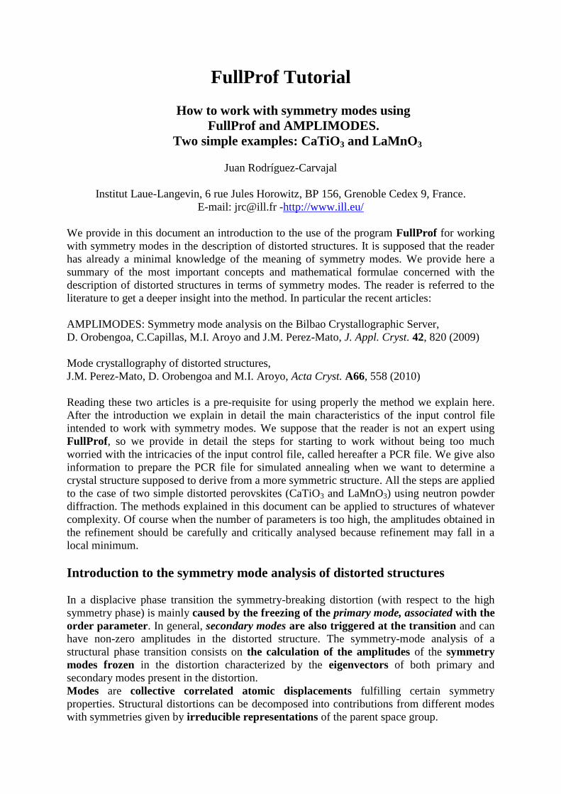
FullProf Tutorial

How to work with symmetry modes using

FullProf and AMPLIMODES.

Two simple examples: CaTiO3 and LaMnO3

Juan Rodríguez-Carvajal

Institut Laue-Langevin, 6 rue Jules Horowitz, BP 156, Grenoble Cedex 9, France.

E-mail: [email protected] -http://www.ill.eu/

We provide in this document an introduction to the use of the program FullProf for working

with symmetry modes in the description of distorted structures. It is supposed that the reader

has already a minimal knowledge of the meaning of symmetry modes. We provide here a

summary of the most important concepts and mathematical formulae concerned with the

description of distorted structures in terms of symmetry modes. The reader is referred to the

literature to get a deeper insight into the method. In particular the recent articles:

AMPLIMODES: Symmetry mode analysis on the Bilbao Crystallographic Server,

D. Orobengoa, C.Capillas, M.I. Aroyo and J.M. Perez-Mato, J. Appl. Cryst. 42, 820 (2009)

Mode crystallography of distorted structures,

J.M. Perez-Mato, D. Orobengoa and M.I. Aroyo, Acta Cryst. A66, 558 (2010)

Reading these two articles is a pre-requisite for using properly the method we explain here.

After the introduction we explain in detail the main characteristics of the input control file

intended to work with symmetry modes. We suppose that the reader is not an expert using

FullProf, so we provide in detail the steps for starting to work without being too much

worried with the intricacies of the input control file, called hereafter a PCR file. We give also

information to prepare the PCR file for simulated annealing when we want to determine a

crystal structure supposed to derive from a more symmetric structure. All the steps are applied

to the case of two simple distorted perovskites (CaTiO3 and LaMnO3) using neutron powder

diffraction. The methods explained in this document can be applied to structures of whatever

complexity. Of course when the number of parameters is too high, the amplitudes obtained in

the refinement should be carefully and critically analysed because refinement may fall in a

local minimum.

Introduction to the symmetry mode analysis of distorted structures

In a displacive phase transition the symmetry-breaking distortion (with respect to the high

symmetry phase) is mainly caused by the freezing of the primary mode, associated with the

order parameter. In general, secondary modes are also triggered at the transition and can

have non-zero amplitudes in the distorted structure. The symmetry-mode analysis of a

structural phase transition consists on the calculation of the amplitudes of the symmetry

modes frozen in the distortion characterized by the eigenvectors of both primary and

secondary modes present in the distortion.

Modes are collective correlated atomic displacements fulfilling certain symmetry

properties. Structural distortions can be decomposed into contributions from different modes

with symmetries given by irreducible representations of the parent space group.

http://www.ill.eu/

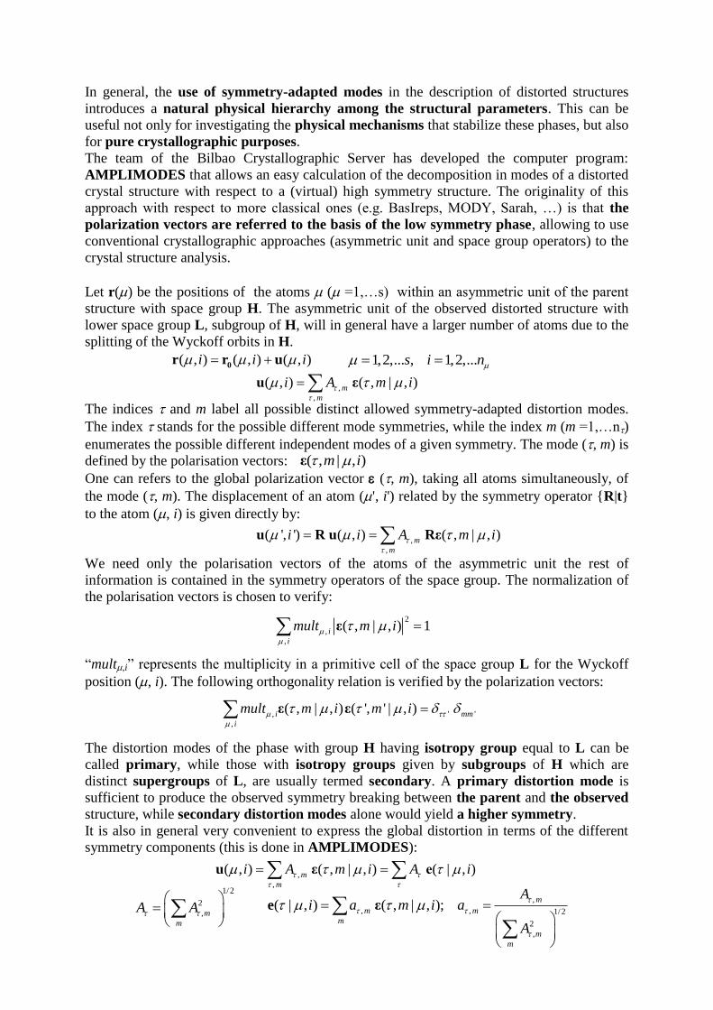
In general, the use of symmetry-adapted modes in the description of distorted structures

introduces a natural physical hierarchy among the structural parameters. This can be

useful not only for investigating the physical mechanisms that stabilize these phases, but also

for pure crystallographic purposes.

The team of the Bilbao Crystallographic Server has developed the computer program:

AMPLIMODES that allows an easy calculation of the decomposition in modes of a distorted

crystal structure with respect to a (virtual) high symmetry structure. The originality of this

approach with respect to more classical ones (e.g. BasIreps, MODY, Sarah, …) is that the

polarization vectors are referred to the basis of the low symmetry phase, allowing to use

conventional crystallographic approaches (asymmetric unit and space group operators) to the

crystal structure analysis.

Let r() be the positions of the atoms ( =1,…s) within an asymmetric unit of the parent

structure with space group H. The asymmetric unit of the observed distorted structure with

lower space group L, subgroup of H, will in general have a larger number of atoms due to the

splitting of the Wyckoff orbits in H.

The indices and m label all possible distinct allowed symmetry-adapted distortion modes.

The index stands for the possible different mode symmetries, while the index m (m =1,…n)

enumerates the possible different independent modes of a given symmetry. The mode (, m) is

defined by the polarisation vectors:

One can refers to the global polarization vector (, m), taking all atoms simultaneously, of

the mode (, m). The displacement of an atom (', i') related by the symmetry operator {R|t}

to the atom (, i) is given directly by:

We need only the polarisation vectors of the atoms of the asymmetric unit the rest of

information is contained in the symmetry operators of the space group. The normalization of

the polarisation vectors is chosen to verify:

“mult,i” represents the multiplicity in a primitive cell of the space group L for the Wyckoff

position (, i). The following orthogonality relation is verified by the polarization vectors:

The distortion modes of the phase with group H having isotropy group equal to L can be

called primary, while those with isotropy groups given by subgroups of H which are

distinct supergroups of L, are usually termed secondary. A primary distortion mode is

sufficient to produce the observed symmetry breaking between the parent and the observed

structure, while secondary distortion modes alone would yield a higher symmetry.

It is also in general very convenient to express the global distortion in terms of the different

symmetry components (this is done in AMPLIMODES):

( , ) ( , ) ( , )0r r ui i i

,

,

( , ) ( , | , )u εm

m

i A m i

1,2,... , 1,2,...s i n

( , | , )ε m i

,

,

( ', ') ( , ) ( , | , )u R u Rεm

m

i i A m i

2

,

,

( , | , ) 1εi

i

mult m i

, ' '

,

( , | , ) ( ', ' | , )ε εi mm

i

mult m i m i

,

,

( , ) ( , | , ) ( | , )u ε em

m

i A m i A i

1/2

2

,m

m

A A

,

, , 1/2

2

,

( | , ) ( , | , );e εm

m m

m

m

m

Ai a m i a

A

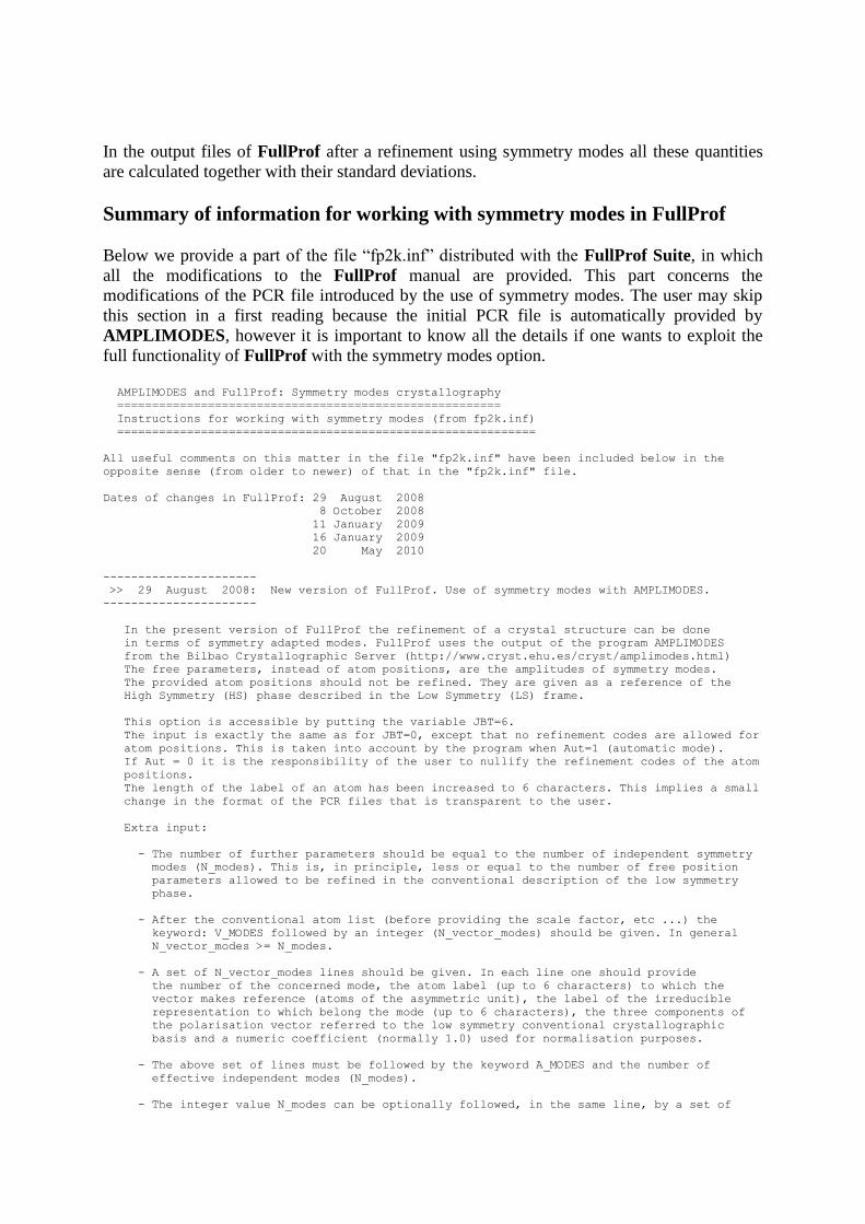
In the output files of FullProf after a refinement using symmetry modes all these quantities

are calculated together with their standard deviations.

Summary of information for working with symmetry modes in FullProf

Below we provide a part of the file “fp2k.inf” distributed with the FullProf Suite, in which

all the modifications to the FullProf manual are provided. This part concerns the

modifications of the PCR file introduced by the use of symmetry modes. The user may skip

this section in a first reading because the initial PCR file is automatically provided by

AMPLIMODES, however it is important to know all the details if one wants to exploit the

full functionality of FullProf with the symmetry modes option.

AMPLIMODES and FullProf: Symmetry modes crystallography

=======================================================

Instructions for working with symmetry modes (from fp2k.inf)

============================================================

All useful comments on this matter in the file "fp2k.inf" have been included below in the

opposite sense (from older to newer) of that in the "fp2k.inf" file.

Dates of changes in FullProf: 29 August 2008

8 October 2008

11 January 2009

16 January 2009

20 May 2010

----------------------

>> 29 August 2008: New version of FullProf. Use of symmetry modes with AMPLIMODES.

----------------------

In the present version of FullProf the refinement of a crystal structure can be done

in terms of symmetry adapted modes. FullProf uses the output of the program AMPLIMODES

from the Bilbao Crystallographic Server (http://www.cryst.ehu.es/cryst/amplimodes.html)

The free parameters, instead of atom positions, are the amplitudes of symmetry modes.

The provided atom positions should not be refined. They are given as a reference of the

High Symmetry (HS) phase described in the Low Symmetry (LS) frame.

This option is accessible by putting the variable JBT=6.

The input is exactly the same as for JBT=0, except that no refinement codes are allowed for

atom positions. This is taken into account by the program when Aut=1 (automatic mode).

If Aut = 0 it is the responsibility of the user to nullify the refinement codes of the atom

positions.

The length of the label of an atom has been increased to 6 characters. This implies a small

change in the format of the PCR files that is transparent to the user.

Extra input:

- The number of further parameters should be equal to the number of independent symmetry

modes (N_modes). This is, in principle, less or equal to the number of free position

parameters allowed to be refined in the conventional description of the low symmetry

phase.

- After the conventional atom list (before providing the scale factor, etc ...) the

keyword: V_MODES followed by an integer (N_vector_modes) should be given. In general

N_vector_modes >= N_modes.

- A set of N_vector_modes lines should be given. In each line one should provide

the number of the concerned mode, the atom label (up to 6 characters) to which the

vector makes reference (atoms of the asymmetric unit), the label of the irreducible

representation to which belong the mode (up to 6 characters), the three components of

the polarisation vector referred to the low symmetry conventional crystallographic

basis and a numeric coefficient (normally 1.0) used for normalisation purposes.

- The above set of lines must be followed by the keyword A_MODES and the number of

effective independent modes (N_modes).

- The integer value N_modes can be optionally followed, in the same line, by a set of

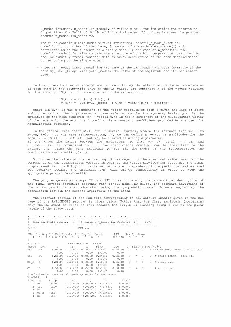
N_modes integers, p_modes(1:N_modes), of values 0 or 1 for indicating the program to

Output files for FullProf Studio of individual modes. If nothing is given the program

assumes p_modes(1:N_modes)=0.

The files contain single modes virtual structures (codefil_n_mode_j.fst for

codefil.pcr, n: number of the phase, j: number of the mode when p_mode(j) = 0)

corresponding to the presence of a single mode. In the case of p_mode(j)=1 the

codefil_n_mode_j.fst file contain the structure of the high temperature (described in

the low symmetry frame) together with an arrow description of the atom displacements

corresponding to the single mode j.

- A set of N_modes lines containing the name of the amplitude parameter (normally of the

form Qj_Label_Irrep, with j=1:N_modes) the value of the amplitude and its refinement

code.

FullProf uses this extra information for calculating the effective fractional coordinates

of each atom in the asymmetric unit of the LS phase. The component k of the vector position

for the atom j, rLS(k,j), is calculated using the expression:

rLS(k,j) = rHS(k,j) + U(k,j)

U(k,j) = Sum{m=1,N_modes} ( Q(m) * vect(k,m,j) * coeff(m) )

Where rHS(k,j) is the k-component of the vector position of atom j given the list of atoms

and correspond to the high symmetry phase referred to the low symmetry basis. Q(m) is the

amplitude of the mode numbered "m", vect(k,m,j) in the k component of the polarisation vector

of the mode m for the atom j and coeff(m) is a constant coefficient provided by the user for

normalisation purposes.

In the general case coeff(m)=1, but if several symmetry modes, for instance from m=i+1 to

m=i+n, belong to the same representation, Dv, we can define a vector of amplitudes for the

form: VQ = {Q(i+1), ...Q(i+n)} that may be treated as a single parameter.

If one knows the ratios between the amplitudes, so that VQ= Qv {r1,r2 .... rn} and

{r1,r2,....rn} is normalized to 1.0, the coefficients coeff(m) can be identified to the

ratios. Then using the same amplitude Qv for all the modes of the representation the

coefficients are: coeff(i+j)= rj.

Of course the values of the refined amplitudes depend on the numerical values used for the

components of the polarisation vectors as well as the values provided for coeff(m). The final

displacement vectors U(k,j) in fractional units are independent of the particular values used

for coeff(m) because the amplitude Q(m) will change consequently in order to keep the

appropriate product Q(m)*coeff(m).

The program generates always CFL and FST files containing the conventional description of

the final crystal structure together with single mode FST files. The standard deviations of

the atoms positions are calculated using the propagation error formula neglecting the

correlation between the refined amplitudes of the modes.

The relevant portion of the PCR file corresponding to the default example given in the Web

page of the AMPLIMODES program is given below. Notice that the first amplitude (concerning

only the Ba atom) is fixed to zero because the origin is floating along z due to the polar

nature of the space group.

. . . . . . . . . . . . . . . . . . . . . . . . . . .

!-------------------------------------------------------------------------------

! Data for PHASE number: 1 ==> Current R_Bragg for Pattern# 1: 0.79

!-------------------------------------------------------------------------------

BaTiO3 FIX xyz

!

!Nat Dis Ang Pr1 Pr2 Pr3 Jbt Irf Isy Str Furth ATZ Nvk Npr More

4 0 0 0.0 0.0 1.0 6 0 0 0 5 967.370 0 7 0

!

A m m 2 <--Space group symbol

!Atom Typ X Y Z Biso Occ In Fin N_t Spc /Codes

Ba1 BA 0.00000 0.00000 0.0000 0.47643 0.25000 0 0 0 1 #color grey conn TI O 0.0 2.2

0.00 0.00 0.00 151.00 0.00

Ti1 TI 0.50000 0.00000 0.50000 0.24156 0.25000 0 0 0 2 # color green poly Ti1

0.00 0.00 0.00 161.00 0.00

O1_2 O 0.00000 0.00000 0.50000 0.58601 0.25000 0 0 0 3 # color cyan

0.00 0.00 0.00 171.00 0.00

O1 O 0.50000 0.25000 0.25000 0.51687 0.50000 0 0 0 3 # color cyan

0.00 0.00 0.00 181.00 0.00

! Polarisation Vectors of Symmetry Modes for each atom

V_MODES 8

! Nm Atm Irrep Vx Vy Vz Coeff

1 Ba1 GM4- 0.000000 0.000000 0.176512 1.00000

2 Ti1 GM4- 0.000000 0.000000 0.176512 1.00000

3 O1 GM4- 0.000000 0.062406 0.062406 1.00000

3 O1_2 GM4- 0.000000 0.000000 0.124813 1.00000

4 O1 GM4- 0.000000 -0.088256 0.088256 1.00000

4 O1_2 GM4- 0.000000 0.000000 0.000000 1.00000

5 O1 GM5- 0.000000 -0.062406 -0.062406 1.00000

5 O1_2 GM5- 0.000000 0.000000 0.124813 1.00000

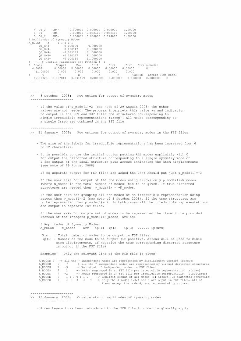
! Amplitudes of Symmetry Modes

A_MODES 5 1 1 1 1 1

Q1_GM4- 0.000000 0.000000

Q2_GM4- 0.098947 21.000000

Q3_GM4- -0.085383 31.000000

Q4_GM4- -0.120367 41.000000

Q5_GM5- -0.006086 51.000000

!-------> Profile Parameters for Pattern # 1

! Scale Shape1 Bov Str1 Str2 Str3 Strain-Model

4.0008 0.00000 0.00000 0.00000 0.00000 0.00000 0

11.00000 0.000 0.000 0.000 0.000 0.000

! U V W X Y GauSiz LorSiz Size-Model

0.176029 -0.197814 0.091459 0.000000 0.030062 0.000000 0.000000 0

. . . . . . . . . . . . . . . . . . . . . . . . . . .

----------------------

>> 8 October 2008: New option for output of symmetry modes

----------------------

- If the value of p_mode(1)=2 (see note of 29 August 2008) the other

values are not needed. The program interprets this value as and indication

to output in the FST and OUT files the structures corresponding to

single irreducible representations (Irrep). All modes corresponding to

a single Irrep are combined in the FST file.

----------------------

>> 11 January 2009: New options for output of symmetry modes in the FST files

----------------------

- The size of the labels for irreducible representations has been increased from 6

to 12 characters.

- It is possible to use the initial option putting ALL modes explicitly with 0

for output the distorted structure corresponding to a single symmetry mode or

1 for output of the ideal structure plus arrows indicating the atom displacements.

(see note of 29 August 2008)

If no separate output for FST files are asked the user should put just p_mode(1)=-3

If the user asks for output of ALL the modes using arrows only p_mode(1)=N_modes

(where N_modes is the total number of modes) has to be given. If true distorted

structures are needed then: p_mode(1) = -N_modes.

If the user asks for grouping all the modes of an irreducible representation using

arrows then p_mode(1)=2 (see note of 8 October 2008), if the true structures are

to be represented then p_mode(1)=-2. In both cases all the irreducible representations

are output in separate FST files.

If the user asks for only a set of modes to be represented the items to be provided

instead of the integers p_mode(1:N_modes) are as:


A_MODES N_modes Nrm ip(1) ip(2) ip(3) ...... ip(Nrm)

Nrm : Total number of modes to be output in FST files

ip(i) : Number of the mode to be output (if positive, arrows will be used to mimic

atom displacements, if negative the true corresponding distorted structure

is output in the FST file)

Examples: (Only the relevant line of the PCR file is given)

A_MODES 7 7 -> all the 7 independent modes are represented by displacement vectors (arrows)

A_MODES 7 -7 -> all the 7 independent modes are represented by virtual distorted structures

A_MODES 7 -3 -> No output of independent modes in FST files

A_MODES 7 2 -> Modes regrouped in an FST file per irreducible representation (arrows)

A_MODES 7 -2 -> Modes regrouped in an FST file per irreducible representation (structures)

A_MODES 7 1 1 1 0 1 1 0 -> Explicit output of all modes (1: arrows, 0: distorted structure)

A_MODES 7 4 1 3 -4 7 -> Only the 4 modes 1,3,4 and 7 are ouput in FST files. All of

them, except the mode 4, are represented by arrows.

----------------------

>> 16 January 2009: Constraints on amplitudes of symmetry modes

----------------------

- A new keyword has been introduced in the PCR file in order to globally apply

a box costraint for the amplitudes of symmetry modes. The keyword is

"Max_Amplitude" and should appear just below the line defining the number

of modes and the output conditions for the FST file. If the keyword does not

appear no constraint is applied to the amplitudes unless Nre /= 0 and the

box constraints on amplitudes are explicitly described. This last method

is needed presently for the simulated annealing mode.

Example:

.....

3 O11 M4- -0.045281 0.045281 0.000000 1.000000


A_MODES 3 2

Max_Amplitude 1.0000

Q1_GM1+ 0.044319 31.000000

Q2_GM1+ -0.158626 41.000000

.....

In the above example the amplitudes (in angstroms) of the symmetry modes are

limited to values within the interval [-1.0, 1.0]

----------------------

>> 20 May 2010: New message in FullProf for symmetry modes.

----------------------

- A stop message is output in FullProf when one uses two phases treated with

symmetry modes in case the second phase has more polarisation vectors than the

first one. For multiphase diffraction patterns to be treated with symmetry

adapted modes, the phase with the greater number of distinct polarisation vectors

should be put as the first phase in the list given in the PCR file.

The initial PCR file obtained automatically from AMPLIMODES

We will illustrate the procedure with the case of the perovskite CaTiO3. We will consider that

we do not know the crystal structure of this material; however we know the unit cell

parameters (a= 5.441Å, b=7.645 Å, c=5.380 Å), the number of formula units Z=4 in the cell,

the space group (Pnma, #62) and the matrix and origin translation relating the orthorhombic

unit cell with that of the cubic high symmetry phase (a-c, 2b, a+c : 000). We know that the

structure derives from the ideal perovskite (Pm3m, #221) containing a single formula unit

with atoms in positions: Ca 1b-(1/2,1/2,1/2), Ti 1a-(0,0,0), O 3d-(1/2,0,0). The cubic cell

parameter of this ideal structure can be obtained from the cell volume of a single formula unit

in the orthorhombic phase: V/4≈223.79/4≈55.95 ac=(V/4)1/3

≈3.8246 Å.

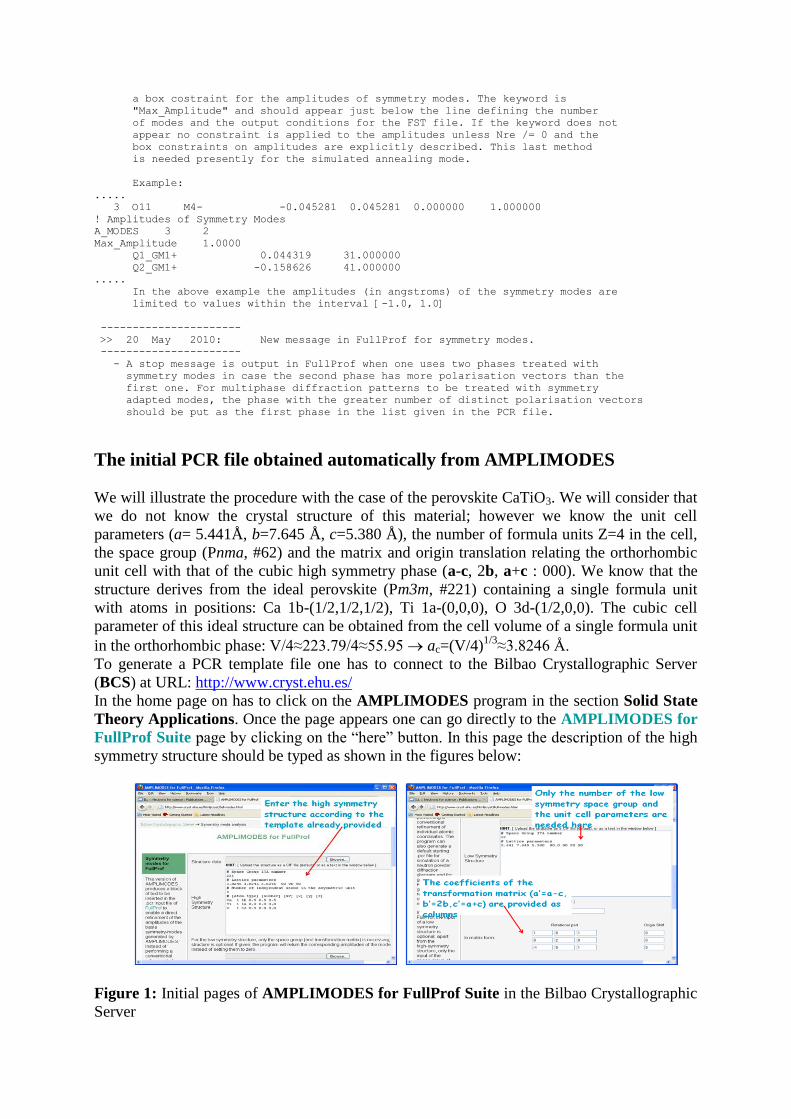
To generate a PCR template file one has to connect to the Bilbao Crystallographic Server

(BCS) at URL: http://www.cryst.ehu.es/

In the home page on has to click on the AMPLIMODES program in the section Solid State

Theory Applications. Once the page appears one can go directly to the AMPLIMODES for

FullProf Suite page by clicking on the “here” button. In this page the description of the high

symmetry structure should be typed as shown in the figures below:

Figure 1: Initial pages of AMPLIMODES for FullProf Suite in the Bilbao Crystallographic

Server

http://www.cryst.ehu.es/

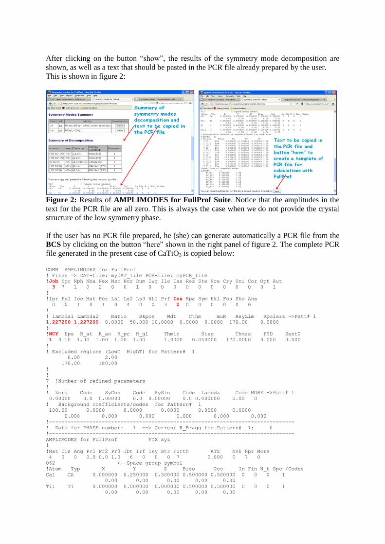
After clicking on the button “show”, the results of the symmetry mode decomposition are

shown, as well as a text that should be pasted in the PCR file already prepared by the user.

This is shown in figure 2:

Figure 2: Results of AMPLIMODES for FullProf Suite. Notice that the amplitudes in the

text for the PCR file are all zero. This is always the case when we do not provide the crystal

structure of the low symmetry phase.

If the user has no PCR file prepared, he (she) can generate automatically a PCR file from the

BCS by clicking on the button “here” shown in the right panel of figure 2. The complete PCR

file generated in the present case of CaTiO3 is copied below:

COMM AMPLIMODES for FullProf

! Files => DAT-file: myDAT_file PCR-file: myPCR_file

!Job Npr Nph Nba Nex Nsc Nor Dum Iwg Ilo Ias Res Ste Nre Cry Uni Cor Opt Aut

3 7 1 0 2 0 0 1 0 0 0 0 0 0 0 0 0 0 1

!

!Ipr Ppl Ioc Mat Pcr Ls1 Ls2 Ls3 NLI Prf Ins Rpa Sym Hkl Fou Sho Ana

0 0 1 0 1 0 4 0 0 3 0 0 0 0 0 0 0

!

! lambda1 Lambda2 Ratio Bkpos Wdt Cthm muR AsyLim Rpolarz ->Patt# 1

1.227200 1.227200 0.0000 50.000 10.0000 0.0000 0.0000 170.00 0.0000

!

!NCY Eps R_at R_an R_pr R_gl Thmin Step Thmax PSD Sent0

1 0.10 1.00 1.00 1.00 1.00 1.0000 0.050000 170.0000 0.000 0.000

!

! Excluded regions (LowT HighT) for Pattern# 1

0.00 2.00

170.00 180.00

!

!

7 !Number of refined parameters

!

! Zero Code SyCos Code SySin Code Lambda Code MORE ->Patt# 1

0.00000 0.0 0.00000 0.0 0.00000 0.0 0.000000 0.00 0

! Background coefficients/codes for Pattern# 1

100.00 0.0000 0.0000 0.0000 0.0000 0.0000

0.000 0.000 0.000 0.000 0.000 0.000

!-------------------------------------------------------------------------------

! Data for PHASE number: 1 ==> Current R_Bragg for Pattern# 1: 0

!-------------------------------------------------------------------------------

AMPLIMODES for FullProf FIX xyz

!


4 0 0 0.0 0.0 1.0 6 0 0 0 7 0.000 0 7 0

062 <--Space group symbol

!Atom Typ X Y Z Biso Occ In Fin N_t Spc /Codes

Ca1 CA 0.000000 0.250000 0.500000 0.500000 0.500000 0 0 0 1

0.00 0.00 0.00 0.00 0.00

Ti1 TI 0.000000 0.000000 0.000000 0.500000 0.500000 0 0 0 1

0.00 0.00 0.00 0.00 0.00

O1 O 0.250000 0.000000 0.250000 0.500000 1.000000 0 0 0 1

0.00 0.00 0.00 0.00 0.00

O1_2 O 0.000000 0.250000 0.000000 0.500000 0.500000 0 0 0 1

0.00 0.00 0.00 0.00 0.00

! Polarisation Vectors of Symmetry Modes for each atom

V_MODES 12

! Nm Atm Irrep Vx Vy Vz Coeff

1 O1 R4+ 0.000000 -0.032683 0.000000 1.00

1 O1_2 R4+ 0.000000 0.000000 0.065366 1.00

2 Ca1 R5+ 0.000000 0.000000 0.092442 1.00

3 O1 R5+ 0.000000 0.032683 0.000000 1.00

3 O1_2 R5+ 0.000000 0.000000 0.065366 1.00

4 Ca1 X5+ 0.092442 0.000000 0.000000 1.00

5 O1 X5+ 0.000000 0.000000 0.000000 1.00

5 O1_2 X5+ -0.092442 0.000000 0.000000 1.00

6 O1 M2+ -0.046221 0.000000 -0.046221 1.00

6 O1_2 M2+ 0.000000 0.000000 0.000000 1.00

7 O1 M3+ 0.046221 0.000000 -0.046221 1.00

7 O1_2 M3+ 0.000000 0.000000 0.000000 1.00

!Amplitudes of Symmetry Modes

A_MODES 7 2

A1_R4+ 0.000000 1.00

A2_R5+ 0.000000 1.00

A3_R5+ 0.000000 1.00

A4_X5+ 0.000000 1.00

A5_X5+ 0.000000 1.00

A6_M2+ 0.000000 1.00

A7_M3+ 0.000000 1.00

!


2.00 0.00000 0.00000 0.00000 0.00000 0.00000 0

0.00000 0.000 0.000 0.000 0.000 0.000


0.176020 -0.197809 0.091458 0.000000 0.030039 0.000000 0.000000 0

0.000 0.000 0.000 0.000 0.000 0.000 0.000

! a b c alpha beta gamma #Cell Info

5.408801 7.649200 5.408801 90.000000 90.000000 90.000000 #box -0.15 1.15 -0.15 1.15 -0.15 1.15

0.00000 0.00000 0.00000 0.00000 0.00000 0.00000

! Pref1 Pref2 Asy1 Asy2 Asy3 Asy4 S_L D_L

0.00000 0.00000 0.00000 0.00000 0.00000 0.00000 0.00000 0.00000

0.00 0.00 0.00 0.00 0.00 0.00 0.00 0.00

! 2Th1/TOF1 2Th2/TOF2 Pattern # 1

10.000 100.000 1

The file above is prepared for the calculation of a neutron diffraction pattern (Jbt=3) similar

to those produced by the instrument 3T2 at Laboratoire Léon Brillouin. The above file may be

used as a template that should be modified for the particular diffraction measurements done

on the sample. We have emphasised in red the variables that have to be eventually modified.

Notice that the cell parameters written in the file correspond to the ideal orthorhombic cell

deduced from the cubic cell applying the transformation matrix given in the input of

AMPLIMODES instead of the real cell parameters. This is so because, strictly speaking, the

orthogonality of the polarisation vectors is verified exactly only in this cell. In practice one

has to write the real cell parameters for refining experimental data.

The file, as produced by AMPLIMODES, can be used for making a calculation with

FullProf. Opening the FullProf Suite toolbar (FPS toolbar), selecting the working directory

(File menu), loading the just created PCR file (left button: Search Input Files) and

clicking on the FullProf button, FullProf is launched. The program processes the input

data and produces files for further inspection and plotting.

In the following figures one can see the process:

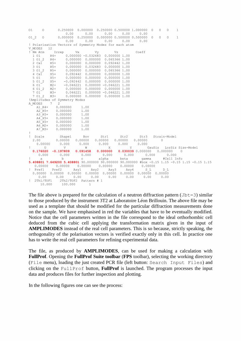
Figure 3: Running FullProf with the “as generated” PCR file (ideal cubic CaTiO3 perovskite,

top left panel) and the file modified using real cell parameters and some reasonable arbitrary

values for the amplitudes of the modes (top right panel). In the bottom panels, pictures of the

atom displacements corresponding to two Irreducible Representations (Irreps) are shown. The

pictures of the left panel are produced automatically when open the FullProf generated files

(*.fst) with FullProf Studio by clicking on the button . The bottom right panel showing

polyhedral representation are generated by editing the *.fst files and adding the instructions:

Conn TI O 0 2.2 and Poly Ti1, after the list of atoms.

The automatically generated PCR-file for CaTiO3 by AMPLIMODES has been called

bcs_template_cti.pcr, and the manually modified file in which we have introduced

the real cell parameters and non-zero reasonable values (lower than 1 Å) for the amplitudes is

called bcs_modified_cti.pcr.

COMM AMPLIMODES for FullProf

! Files => DAT-file: myDAT_file PCR-file: myPCR_file


3 7 1 0 2 0 0 1 0 0 0 0 0 0 0 0 0 0 1

!


0 0 1 0 1 0 4 0 0 3 0 0 0 0 0 0 0

!


1.227200 1.227200 0.0000 50.000 10.0000 0.0000 0.0000 170.00 0.0000

!


1 0.10 1.00 1.00 1.00 1.00 1.0000 0.050000 170.0000 0.000 0.000

!


0.00 2.00

170.00 180.00

!

!


!


0.00000 0.0 0.00000 0.0 0.00000 0.0 0.000000 0.00 0

!-------------------------------------------------------------------------------

! Data for PHASE number: 1 ==> Current R_Bragg for Pattern# 1: 0

!-------------------------------------------------------------------------------

AMPLIMODES for FullProf FIX xyz

!


0 0 0 0.0 0.0 1.0 6 0 0 0 7 0.000 0 7 0

062 <--Space group symbol


2.00 0.00000 0.00000 0.00000 0.00000 0.00000 0

0.00000 0.000 0.000 0.000 0.000 0.000


0.176020 -0.197809 0.091458 0.000000 0.030039 0.000000 0.000000 0

0.000 0.000 0.000 0.000 0.000 0.000 0.000


5.408801 7.649200 5.408801 90.000000 90.000000 90.000000 #box -0.15 1.15 -0.15 1.15 -0.15 1.15

0.00000 0.00000 0.00000 0.00000 0.00000 0.00000

. . . . . .

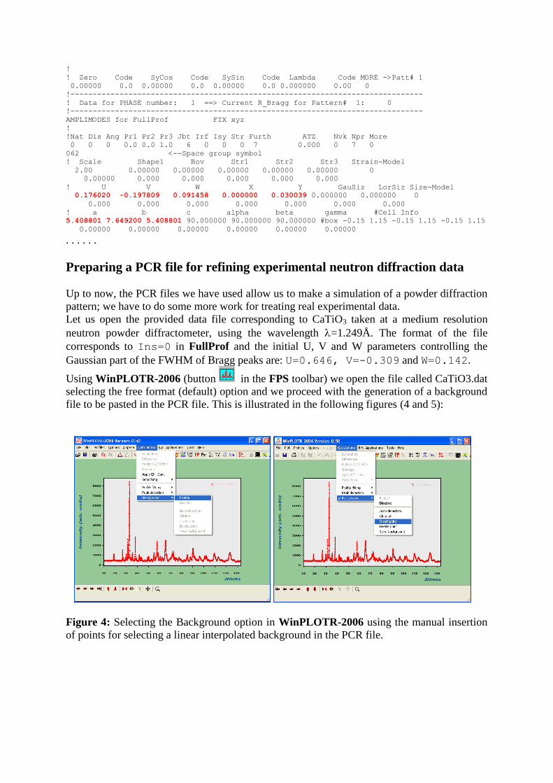
Preparing a PCR file for refining experimental neutron diffraction data

Up to now, the PCR files we have used allow us to make a simulation of a powder diffraction

pattern; we have to do some more work for treating real experimental data.

Let us open the provided data file corresponding to CaTiO3 taken at a medium resolution

neutron powder diffractometer, using the wavelength =1.249Å. The format of the file

corresponds to Ins=0 in FullProf and the initial U, V and W parameters controlling the

Gaussian part of the FWHM of Bragg peaks are: U=0.646, V=-0.309 and W=0.142.

Using WinPLOTR-2006 (button in the FPS toolbar) we open the file called CaTiO3.dat

selecting the free format (default) option and we proceed with the generation of a background

file to be pasted in the PCR file. This is illustrated in the following figures (4 and 5):

Figure 4: Selecting the Background option in WinPLOTR-2006 using the manual insertion

of points for selecting a linear interpolated background in the PCR file.

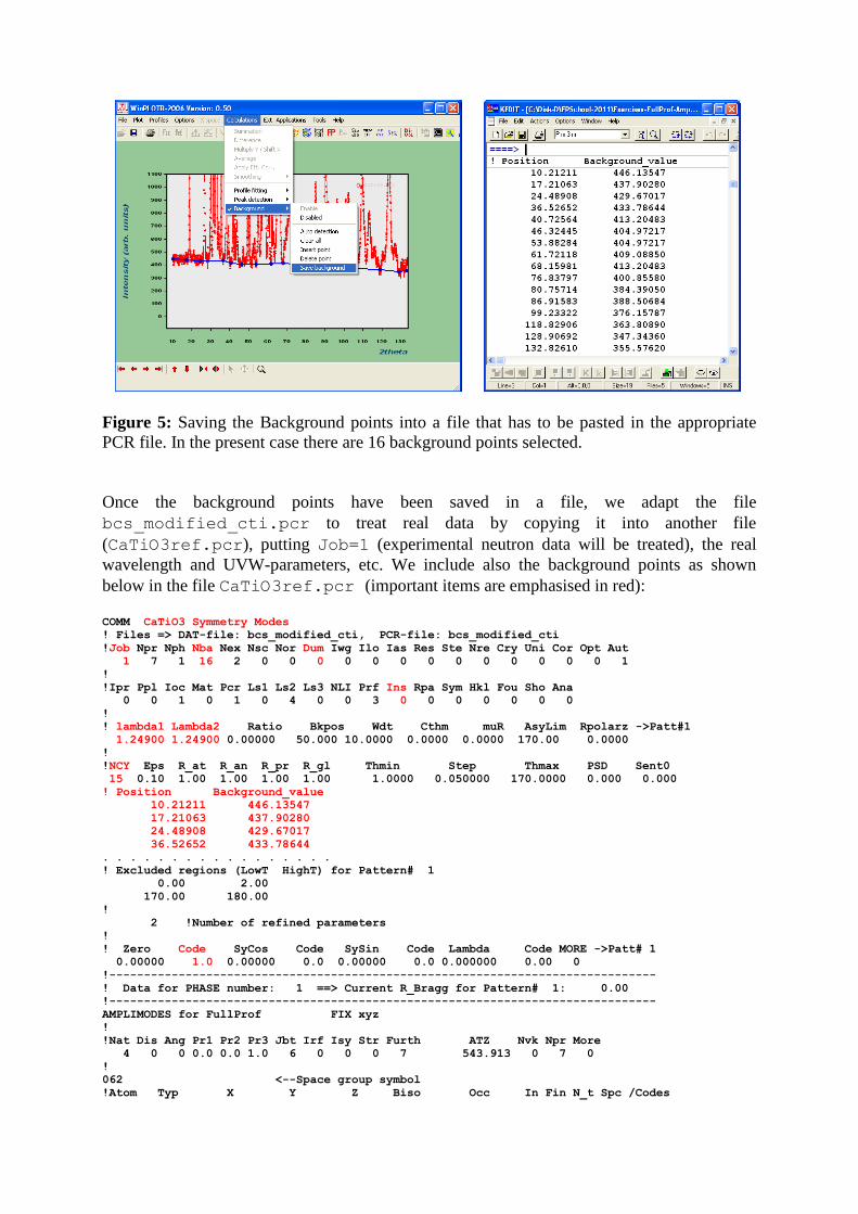
Figure 5: Saving the Background points into a file that has to be pasted in the appropriate

PCR file. In the present case there are 16 background points selected.

Once the background points have been saved in a file, we adapt the file

bcs_modified_cti.pcr to treat real data by copying it into another file

(CaTiO3ref.pcr), putting Job=1 (experimental neutron data will be treated), the real

wavelength and UVW-parameters, etc. We include also the background points as shown

below in the file CaTiO3ref.pcr (important items are emphasised in red):

COMM CaTiO3 Symmetry Modes ! Files => DAT-file: bcs_modified_cti, PCR-file: bcs_modified_cti

!Job Npr Nph Nba Nex Nsc Nor Dum Iwg Ilo Ias Res Ste Nre Cry Uni Cor Opt Aut 1 7 1 16 2 0 0 0 0 0 0 0 0 0 0 0 0 0 1 ! !Ipr Ppl Ioc Mat Pcr Ls1 Ls2 Ls3 NLI Prf Ins Rpa Sym Hkl Fou Sho Ana 0 0 1 0 1 0 4 0 0 3 0 0 0 0 0 0 0 ! ! lambda1 Lambda2 Ratio Bkpos Wdt Cthm muR AsyLim Rpolarz ->Patt#1 1.24900 1.24900 0.00000 50.000 10.0000 0.0000 0.0000 170.00 0.0000 ! !NCY Eps R_at R_an R_pr R_gl Thmin Step Thmax PSD Sent0 15 0.10 1.00 1.00 1.00 1.00 1.0000 0.050000 170.0000 0.000 0.000 ! Position Background_value 10.21211 446.13547 17.21063 437.90280 24.48908 429.67017 36.52652 433.78644 . . . . . . . . . . . . . . . . . ! Excluded regions (LowT HighT) for Pattern# 1 0.00 2.00

170.00 180.00 ! 2 !Number of refined parameters ! ! Zero Code SyCos Code SySin Code Lambda Code MORE ->Patt# 1 0.00000 1.0 0.00000 0.0 0.00000 0.0 0.000000 0.00 0 !------------------------------------------------------------------------------- ! Data for PHASE number: 1 ==> Current R_Bragg for Pattern# 1: 0.00 !------------------------------------------------------------------------------- AMPLIMODES for FullProf FIX xyz ! !Nat Dis Ang Pr1 Pr2 Pr3 Jbt Irf Isy Str Furth ATZ Nvk Npr More 4 0 0 0.0 0.0 1.0 6 0 0 0 7 543.913 0 7 0 ! 062 <--Space group symbol !Atom Typ X Y Z Biso Occ In Fin N_t Spc /Codes

Ca1 CA 0.00000 0.25000 0.50000 0.50000 0.50000 0 0 0 1 0.00 0.00 0.00 0.00 0.00 Ti1 TI 0.00000 0.00000 0.00000 0.50000 0.50000 0 0 0 1 0.00 0.00 0.00 0.00 0.00 . . . . . . . . . . . . 7 O1 M3+ 0.046221 0.000000 -0.046221 1.000000 7 O1_2 M3+ 0.000000 0.000000 0.000000 1.000000 ! Amplitudes of Symmetry Modes A_MODES 7 2 A1_R4+ 0.800000 .000000 A2_R5+ -0.100000 .000000 A3_R5+ 0.300000 .000000 A4_X5+ 0.700000 .000000 A5_X5+ 0.100000 .000000 A6_M2+ 0.020000 .000000 A7_M3+ 0.100000 .000000 !-------> Profile Parameters for Pattern # 1 ! Scale Shape1 Bov Str1 Str2 Str3 Strain-Model 1.0000 0.00000 0.00000 0.00000 0.00000 0.00000 0 1.00000 0.000 0.000 0.000 0.000 0.000 ! U V W X Y GauSiz LorSiz Size-Model 0.64600 -0.309000 0.142000 0.000000 0.000000 0.000000 0.000000 0 0.000 0.000 0.000 0.000 0.000 0.000 0.000 ! a b c alpha beta gamma #Cell Info 5.441000 7.645000 5.380000 90.000000 90.000000 90.000000 0.00000 0.00000 0.00000 0.00000 0.00000 0.00000 . . .

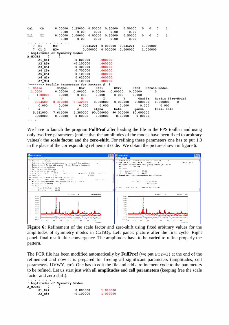
We have to launch the program FullProf after loading the file in the FPS toolbar and using

only two free parameters (notice that the amplitudes of the modes have been fixed to arbitrary

values): the scale factor and the zero-shift. For refining these parameters one has to put 1.0

in the place of the corresponding refinement code. We obtain the picture shown in figure 6:

Figure 6: Refinement of the scale factor and zero-shift using fixed arbitrary values for the

amplitudes of symmetry modes in CaTiO3. Left panel: picture after the first cycle. Right

panel: final result after convergence. The amplitudes have to be varied to refine properly the

pattern.

The PCR file has been modified automatically by FullProf (we put Pcr=1) at the end of the

refinement and now it is prepared for freeing all significant parameters (amplitudes, cell

parameters, UVWY, etc). One has to edit the file and add a refinement code to the parameters

to be refined. Let us start just with all amplitudes and cell parameters (keeping free the scale

factor and zero-shift). . . . . . . .


A_MODES 7 2

A1_R4+ 0.800000 1.000000

A2_R5+ -0.100000 1.000000

A3_R5+ 0.300000 1.000000

A4_X5+ 0.700000 1.000000

A5_X5+ 0.100000 1.000000

A6_M2+ 0.020000 1.000000

A7_M3+ 0.100000 1.000000



0.90509 0.00000 0.00000 0.00000 0.00000 0.00000 0

21.00000 0.000 0.000 0.000 0.000 0.000


0.646000 -0.309000 0.142000 0.000000 0.000000 0.000000 0.000000 0

0.000 0.000 0.000 0.000 0.000 0.000 0.000


5.441000 7.645000 5.380000 90.000000 90.000000 90.000000

0.00000 0.00000 0.00000 0.00000 0.00000 0.00000

. . . . . . .

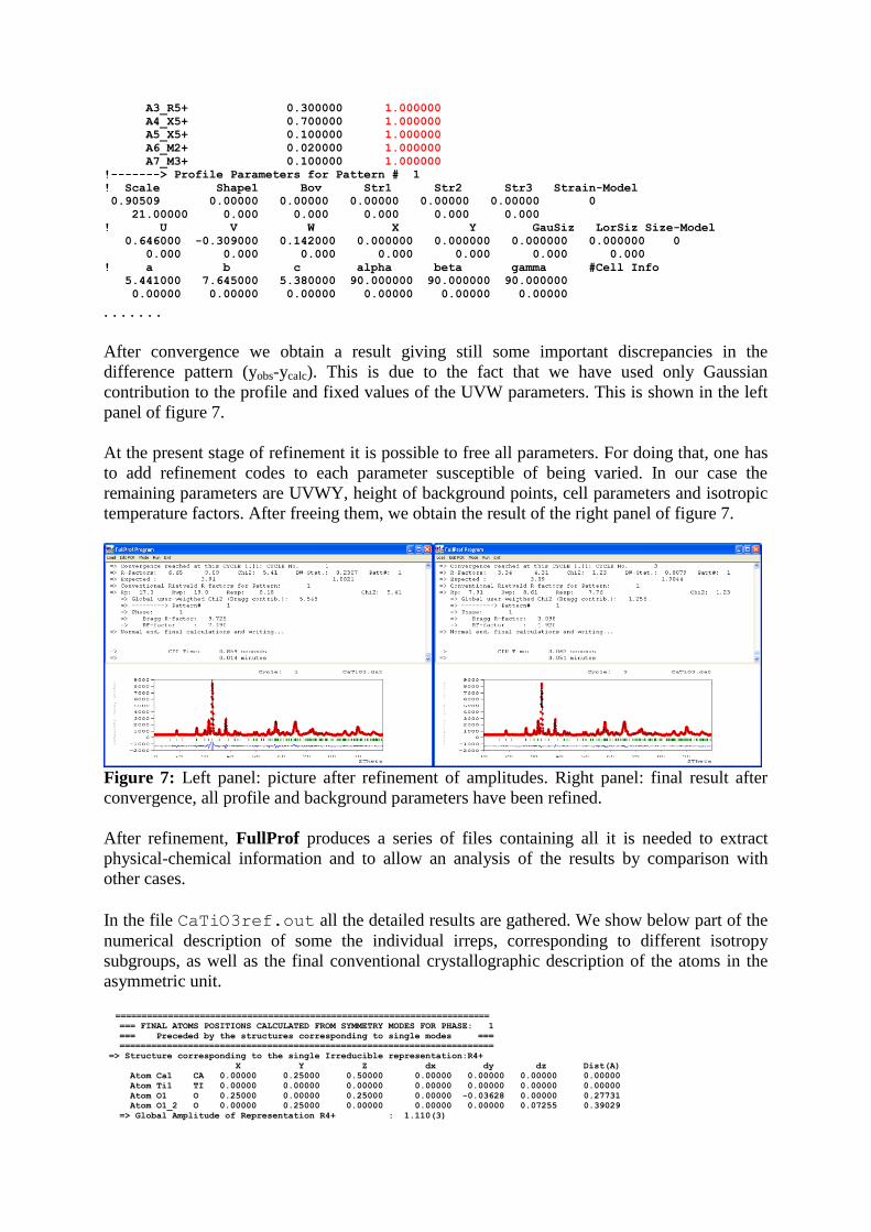
After convergence we obtain a result giving still some important discrepancies in the

difference pattern (yobs-ycalc). This is due to the fact that we have used only Gaussian

contribution to the profile and fixed values of the UVW parameters. This is shown in the left

panel of figure 7.

At the present stage of refinement it is possible to free all parameters. For doing that, one has

to add refinement codes to each parameter susceptible of being varied. In our case the

remaining parameters are UVWY, height of background points, cell parameters and isotropic

temperature factors. After freeing them, we obtain the result of the right panel of figure 7.

Figure 7: Left panel: picture after refinement of amplitudes. Right panel: final result after

convergence, all profile and background parameters have been refined.

After refinement, FullProf produces a series of files containing all it is needed to extract

physical-chemical information and to allow an analysis of the results by comparison with

other cases.

In the file CaTiO3ref.out all the detailed results are gathered. We show below part of the

numerical description of some the individual irreps, corresponding to different isotropy

subgroups, as well as the final conventional crystallographic description of the atoms in the

asymmetric unit.

======================================================================= === FINAL ATOMS POSITIONS CALCULATED FROM SYMMETRY MODES FOR PHASE: 1

=== Preceded by the structures corresponding to single modes ===

=======================================================================

=> Structure corresponding to the single Irreducible representation:R4+

X Y Z dx dy dz Dist(A)

Atom Ca1 CA 0.00000 0.25000 0.50000 0.00000 0.00000 0.00000 0.00000

Atom Ti1 TI 0.00000 0.00000 0.00000 0.00000 0.00000 0.00000 0.00000

Atom O1 O 0.25000 0.00000 0.25000 0.00000 -0.03628 0.00000 0.27731

Atom O1_2 O 0.00000 0.25000 0.00000 0.00000 0.00000 0.07255 0.39029

=> Global Amplitude of Representation R4+ : 1.110(3)

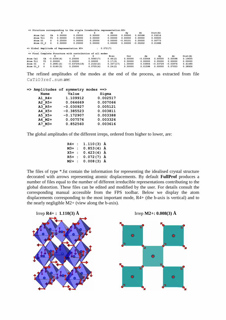
=> Structure corresponding to the single Irreducible representation:R5+

X Y Z dx dy dz Dist(A)

Atom Ca1 CA 0.00000 0.25000 0.50000 0.00000 0.00000 0.00598 0.03216

Atom Ti1 TI 0.00000 0.00000 0.00000 0.00000 0.00000 0.00000 0.00000

Atom O1 O 0.25000 0.00000 0.25000 0.00000 -0.00101 0.00000 0.00773

Atom O1_2 O 0.00000 0.25000 0.00000 0.00000 0.00000 -0.00202 0.01088


. . . . . . . . . .

=> Final Complete Structure with contribution of all modes

X Y Z Biso Occ dx dy dz Dist(A)

Atom Ca1 CA -0.0356(4) 0.25000 0.5060(7) 0.46(2) 0.50000 -0.03564 0.00000 0.00598 0.19655

Atom Ti1 TI 0.00000 0.00000 0.00000 0.17(3) 0.50000 0.00000 0.00000 0.00000 0.00000

Atom O1 O 0.2891(2) -0.03729(19) 0.2102(2) 0.337(17) 1.00000 0.03906 -0.03729 -0.03976 0.41490

Atom O1_2 O 0.0160(3) 0.25000 0.0705(4) 0.24(2) 0.50000 0.01598 0.00000 0.07053 0.38926

The refined amplitudes of the modes at the end of the process, as extracted from file

CaTiO3ref.sum are:

=> Amplitudes of symmetry modes ==>

Name Value Sigma

A1_R4+ 1.109912 0.002517

A2_R5+ 0.064669 0.007066

A3_R5+ -0.030927 0.005121

A4_X5+ -0.385523 0.003811

A5_X5+ -0.172907 0.003388

A6_M2+ 0.007576 0.003326

A7_M3+ 0.852560 0.003616

The global amplitudes of the different irreps, ordered from higher to lower, are:

R4+ : 1.110(3) Å

M3+ : 0.853(4) Å

X5+ : 0.423(4) Å

R5+ : 0.072(7) Å

M2+ : 0.008(3) Å

The files of type *.fst contain the information for representing the idealised crystal structure

decorated with arrows representing atomic displacements. By default FullProf produces a

number of files equal to the number of different irreducible representations contributing to the

global distortion. These files can be edited and modified by the user. For details consult the

corresponding manual accessible from the FPS toolbar. Below we display the atom

displacements corresponding to the most important mode, R4+ (the b-axis is vertical) and to

the nearly negligible M2+ (view along the b-axis).

Irrep R4+ : 1.110(3) Å Irrep M2+: 0.008(3) Å

Preparing a PCR file for extracting integrated intensities and generate files

to be used by the Simulated Annealing option of FullProf

The process we have shown up to now goes directly to the refinement of amplitudes starting

with an arbitrary initial set. This works for the case of CaTiO3 because it is a simple structure

with only seven degrees of freedom.

In the general case one has to be able to “solve” nearly ab initio a crystal structure supposed

to derive from another of higher symmetry. For that a global optimisation method (as opposed

to least squares, which is local) may be necessary for getting good initial values for the

amplitudes.

Extracting integrated intensities or structure factors from powder diffraction data, once we

know the unit cell parameters, is straightforward in well crystallised samples; however there

are cases where the tasks may be complicated due to the presence of broadening due to micro-

structural effects. To avoid, from the beginning, pitfalls due to the handling of full width at

half maximum it is convenient to work with instrumental resolution function files. This has as

an additional advantage the production of micro-structural files containing information about

the size and strain effects of your sample.

The procedure used for extracting the integrated intensities within FullProf (profile matching)

is currently known as Le Bail fitting [A. LeBail, H. Duroy and J.L. Fourquet, Mat. Res. Bull.

23, 447(1988)]. It does not require any structural information except approximate unit cell and

resolution parameters. A similar method developed by Pawley uses traditional least squares

with constraints [G.S. Pawley, J. Applied Cryst. 14, 357 (1981)]. A discussion about the

profile matching algorithm involved in this kind of refinement may be found in [J. Rodríguez-

Carvajal, Physica B 192, 55 (1993)]. This method makes the data input much simpler and

enlarges considerably the field of application of powder pattern profile refinement. However

the constraints applied to the refinement are far less severe than for Rietveld refinement and

profile matching is thereby more prone to instabilities if profile shape parameters or micro-

structural parameters are refined.

The Le Bail Fit (LBF) with constant scale factor is accessible by putting (Jbt=2). In this

mode the scale factor is not allowed to vary and integrated intensities are refined individually

using iteratively the Rietveld formula for obtaining the integrated observed intensity. The

recommended procedure is as follows:

For the first refinement, set IRF(n) of the phase n undergoing profile matching to 0

and the number of refined parameters (MAXS on line 13) to zero. Set to 0 the flag

controlling the automatic assignment of refinement codes (Aut=0). Run FullProf for

a few cycles (say 10). This will set up the hkl 's and intensity file CODFILn.hkl.

If the result of the above step is satisfactory (see plot!), rename the file CODFIL.new

to CODFIL.pcr, or use directly CODFIL.pcr if it was automatically updated. Edit

the new CODFIL.pcr file to select the parameters to refine. The progression of the

refinement is very similar to that used for Rietveld refinement: zero-shift of detector,

background parameters and lattice constants.

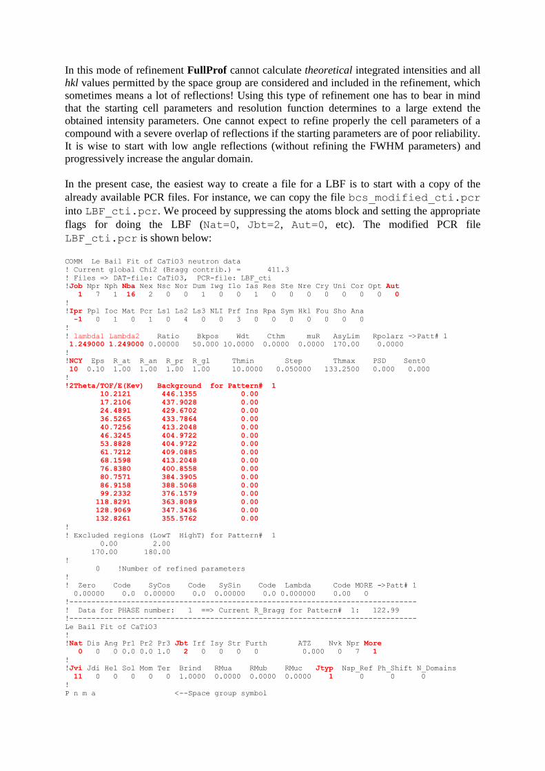
In this mode of refinement FullProf cannot calculate theoretical integrated intensities and all

hkl values permitted by the space group are considered and included in the refinement, which

sometimes means a lot of reflections! Using this type of refinement one has to bear in mind

that the starting cell parameters and resolution function determines to a large extend the

obtained intensity parameters. One cannot expect to refine properly the cell parameters of a

compound with a severe overlap of reflections if the starting parameters are of poor reliability.

It is wise to start with low angle reflections (without refining the FWHM parameters) and

progressively increase the angular domain.

In the present case, the easiest way to create a file for a LBF is to start with a copy of the

already available PCR files. For instance, we can copy the file bcs_modified_cti.pcr

into LBF_cti.pcr. We proceed by suppressing the atoms block and setting the appropriate

flags for doing the LBF (Nat=0, Jbt=2, Aut=0, etc). The modified PCR file

LBF_cti.pcr is shown below:

COMM Le Bail Fit of CaTiO3 neutron data

! Current global Chi2 (Bragg contrib.) = 411.3

! Files => DAT-file: CaTiO3, PCR-file: LBF_cti


1 7 1 16 2 0 0 1 0 0 1 0 0 0 0 0 0 0 0

!


-1 0 1 0 1 0 4 0 0 3 0 0 0 0 0 0 0

!


1.249000 1.249000 0.00000 50.000 10.0000 0.0000 0.0000 170.00 0.0000

!


10 0.10 1.00 1.00 1.00 1.00 10.0000 0.050000 133.2500 0.000 0.000

!

!2Theta/TOF/E(Kev) Background for Pattern# 1

10.2121 446.1355 0.00

17.2106 437.9028 0.00

24.4891 429.6702 0.00

36.5265 433.7864 0.00

40.7256 413.2048 0.00

46.3245 404.9722 0.00

53.8828 404.9722 0.00

61.7212 409.0885 0.00

68.1598 413.2048 0.00

76.8380 400.8558 0.00

80.7571 384.3905 0.00

86.9158 388.5068 0.00

99.2332 376.1579 0.00

118.8291 363.8089 0.00

128.9069 347.3436 0.00

132.8261 355.5762 0.00

!


0.00 2.00

170.00 180.00

!


!


0.00000 0.0 0.00000 0.0 0.00000 0.0 0.000000 0.00 0

!-------------------------------------------------------------------------------

! Data for PHASE number: 1 ==> Current R_Bragg for Pattern# 1: 122.99

!-------------------------------------------------------------------------------

Le Bail Fit of CaTiO3

!


0 0 0 0.0 0.0 1.0 2 0 0 0 0 0.000 0 7 1

!

!Jvi Jdi Hel Sol Mom Ter Brind RMua RMub RMuc Jtyp Nsp_Ref Ph_Shift N_Domains

11 0 0 0 0 0 1.0000 0.0000 0.0000 0.0000 1 0 0 0

!

P n m a <--Space group symbol



1.0000 0.00000 0.00000 0.00000 0.00000 0.00000 0

0.00000 0.000 0.000 0.000 0.000 0.000


0.646000 -0.309000 0.142000 0.000000 0.000000 0.000000 0.000000 0

0.000 0.000 0.000 0.000 0.000 0.000 0.000


5.441000 7.645000 5.380000 90.000000 90.000000 90.000000

0.00000 0.00000 0.00000 0.00000 0.00000 0.00000

! Pref1 Pref2 Asy1 Asy2 Asy3 Asy4 S_L D_L

. . . . . . . . . .

All the important flags that we have modified are emphasised in red. The polynomial

background parameters have been deleted and replaced by the background points determined

with the help of WinPLOTR-2006. The flag Ipr=-1 means that after the LBF a file

containing information on profile intensity contributions will be generated (called

LBF_cti.spr). The flag Jvi=11 means that a file with integrated intensity clusters is output

(LBF_cti1_cltr.int). Both files will be used later for doing a simulated annealing

search of the amplitudes.

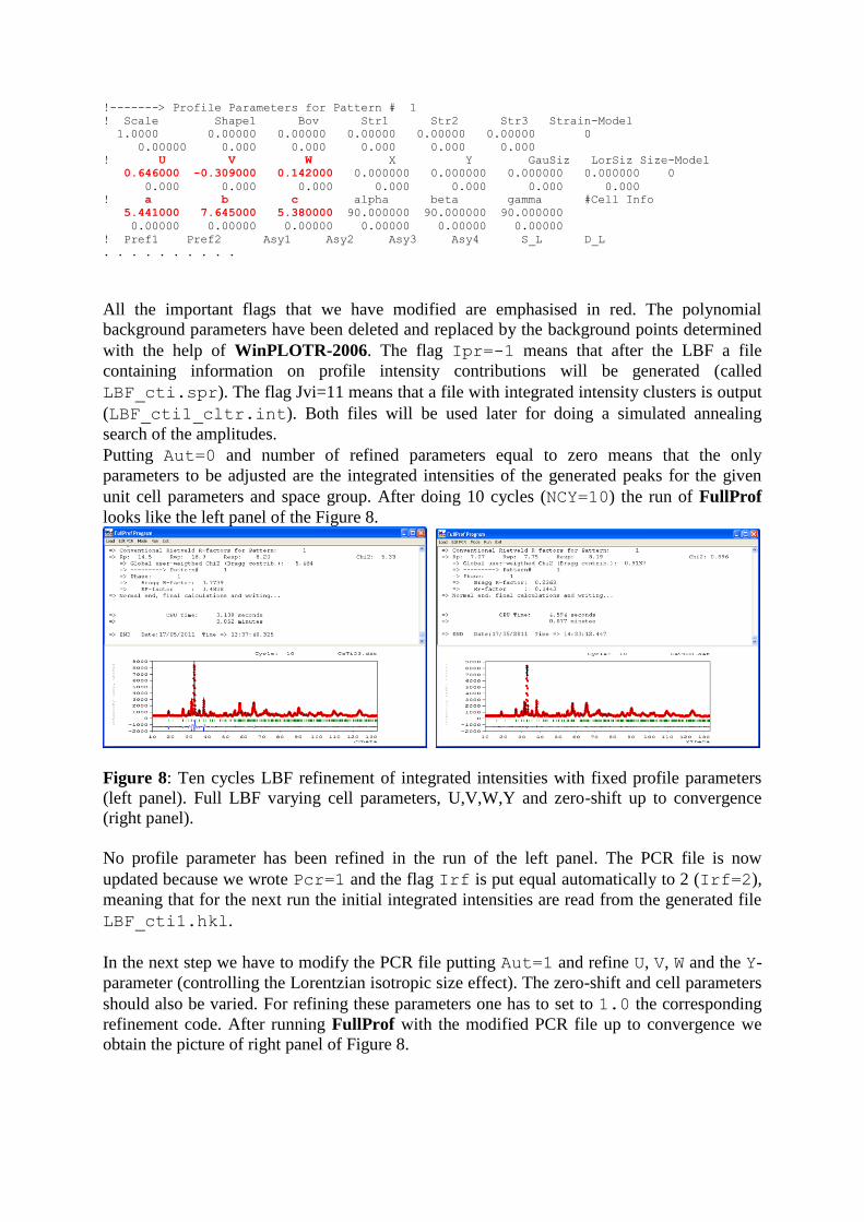
Putting Aut=0 and number of refined parameters equal to zero means that the only

parameters to be adjusted are the integrated intensities of the generated peaks for the given

unit cell parameters and space group. After doing 10 cycles (NCY=10) the run of FullProf

looks like the left panel of the Figure 8.

Figure 8: Ten cycles LBF refinement of integrated intensities with fixed profile parameters

(left panel). Full LBF varying cell parameters, U,V,W,Y and zero-shift up to convergence

(right panel).

No profile parameter has been refined in the run of the left panel. The PCR file is now

updated because we wrote Pcr=1 and the flag Irf is put equal automatically to 2 (Irf=2),

meaning that for the next run the initial integrated intensities are read from the generated file

LBF_cti1.hkl.

In the next step we have to modify the PCR file putting Aut=1 and refine U, V, W and the Y-

parameter (controlling the Lorentzian isotropic size effect). The zero-shift and cell parameters

should also be varied. For refining these parameters one has to set to 1.0 the corresponding

refinement code. After running FullProf with the modified PCR file up to convergence we

obtain the picture of right panel of Figure 8.

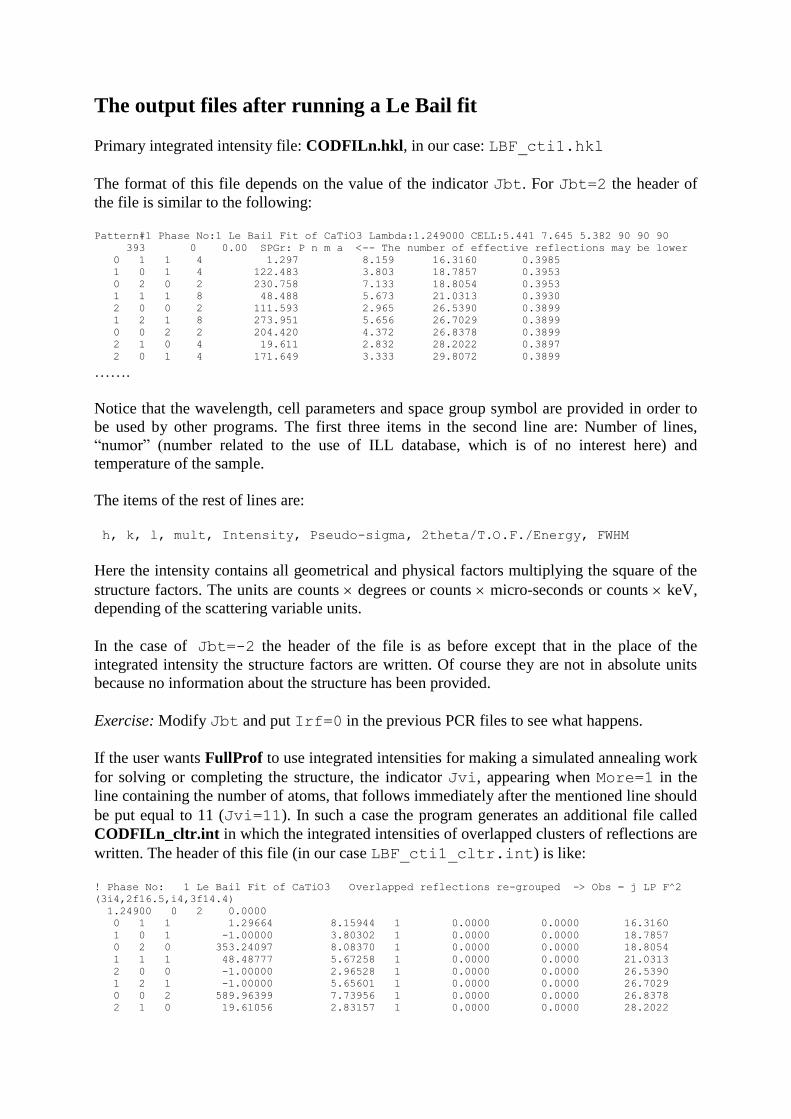
The output files after running a Le Bail fit

Primary integrated intensity file: CODFILn.hkl, in our case: LBF_cti1.hkl

The format of this file depends on the value of the indicator Jbt. For Jbt=2 the header of

the file is similar to the following:

Pattern#1 Phase No:1 Le Bail Fit of CaTiO3 Lambda:1.249000 CELL:5.441 7.645 5.382 90 90 90

393 0 0.00 SPGr: P n m a <-- The number of effective reflections may be lower

0 1 1 4 1.297 8.159 16.3160 0.3985

1 0 1 4 122.483 3.803 18.7857 0.3953

0 2 0 2 230.758 7.133 18.8054 0.3953

1 1 1 8 48.488 5.673 21.0313 0.3930

2 0 0 2 111.593 2.965 26.5390 0.3899

1 2 1 8 273.951 5.656 26.7029 0.3899

0 0 2 2 204.420 4.372 26.8378 0.3899

2 1 0 4 19.611 2.832 28.2022 0.3897

2 0 1 4 171.649 3.333 29.8072 0.3899

…….

Notice that the wavelength, cell parameters and space group symbol are provided in order to

be used by other programs. The first three items in the second line are: Number of lines,

“numor” (number related to the use of ILL database, which is of no interest here) and

temperature of the sample.

The items of the rest of lines are:

h, k, l, mult, Intensity, Pseudo-sigma, 2theta/T.O.F./Energy, FWHM

Here the intensity contains all geometrical and physical factors multiplying the square of the

structure factors. The units are counts degrees or counts micro-seconds or counts keV,

depending of the scattering variable units.

In the case of Jbt=-2 the header of the file is as before except that in the place of the

integrated intensity the structure factors are written. Of course they are not in absolute units

because no information about the structure has been provided.

Exercise: Modify Jbt and put Irf=0 in the previous PCR files to see what happens.

If the user wants FullProf to use integrated intensities for making a simulated annealing work

for solving or completing the structure, the indicator Jvi, appearing when More=1 in the

line containing the number of atoms, that follows immediately after the mentioned line should

be put equal to 11 (Jvi=11). In such a case the program generates an additional file called

CODFILn_cltr.int in which the integrated intensities of overlapped clusters of reflections are

written. The header of this file (in our case LBF_cti1_cltr.int) is like:

! Phase No: 1 Le Bail Fit of CaTiO3 Overlapped reflections re-grouped -> Obs = j LP F^2

(3i4,2f16.5,i4,3f14.4)

1.24900 0 2 0.0000

0 1 1 1.29664 8.15944 1 0.0000 0.0000 16.3160

1 0 1 -1.00000 3.80302 1 0.0000 0.0000 18.7857

0 2 0 353.24097 8.08370 1 0.0000 0.0000 18.8054

1 1 1 48.48777 5.67258 1 0.0000 0.0000 21.0313

2 0 0 -1.00000 2.96528 1 0.0000 0.0000 26.5390

1 2 1 -1.00000 5.65601 1 0.0000 0.0000 26.7029

0 0 2 589.96399 7.73956 1 0.0000 0.0000 26.8378

2 1 0 19.61056 2.83157 1 0.0000 0.0000 28.2022

2 0 1 -1.00000 3.33281 1 0.0000 0.0000 29.8072

1 0 2 399.24738 5.05503 1 0.0000 0.0000 30.0091

2 1 1 -1.00000 3.22797 1 0.0000 0.0000 31.3112

0 3 1 -1.00000 1.17173 1 0.0000 0.0000 31.4644

1 1 2 1100.58142 6.09536 1 0.0000 0.0000 31.5043

…… .....

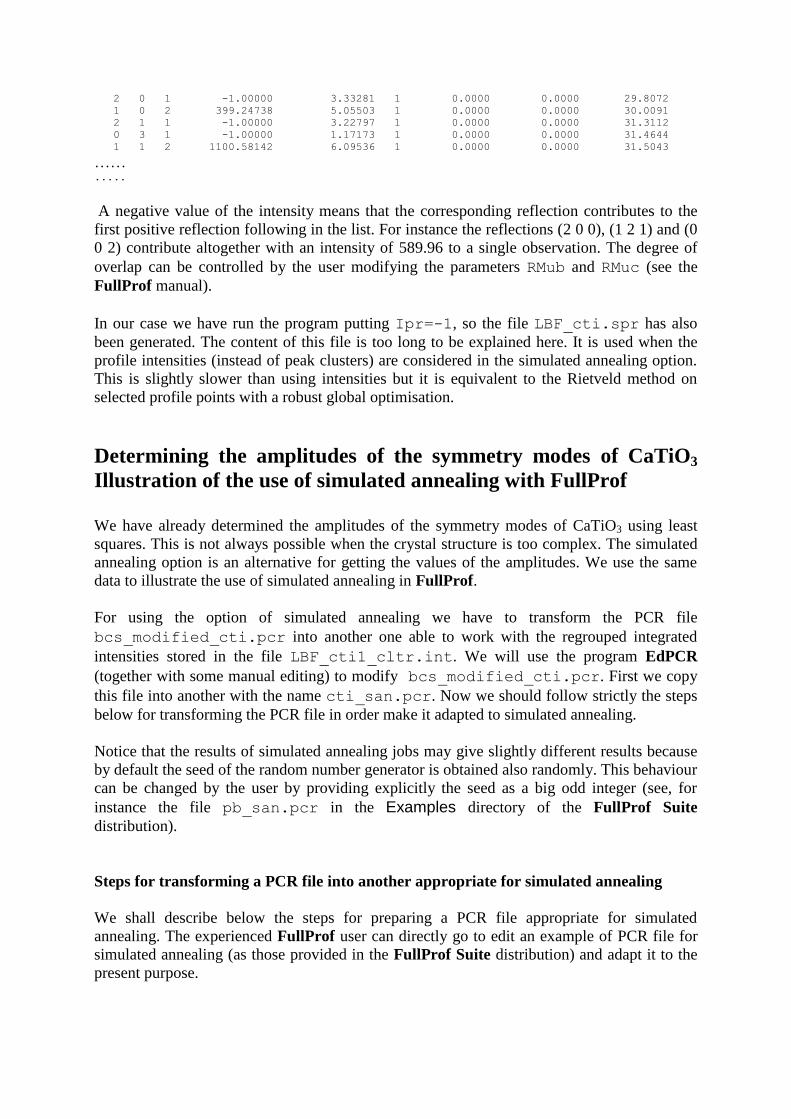
A negative value of the intensity means that the corresponding reflection contributes to the

first positive reflection following in the list. For instance the reflections (2 0 0), (1 2 1) and (0

0 2) contribute altogether with an intensity of 589.96 to a single observation. The degree of

overlap can be controlled by the user modifying the parameters RMub and RMuc (see the

FullProf manual).

In our case we have run the program putting Ipr=-1, so the file LBF_cti.spr has also

been generated. The content of this file is too long to be explained here. It is used when the

profile intensities (instead of peak clusters) are considered in the simulated annealing option.

This is slightly slower than using intensities but it is equivalent to the Rietveld method on

selected profile points with a robust global optimisation.

Determining the amplitudes of the symmetry modes of CaTiO3

Illustration of the use of simulated annealing with FullProf

We have already determined the amplitudes of the symmetry modes of CaTiO3 using least

squares. This is not always possible when the crystal structure is too complex. The simulated

annealing option is an alternative for getting the values of the amplitudes. We use the same

data to illustrate the use of simulated annealing in FullProf.

For using the option of simulated annealing we have to transform the PCR file

bcs_modified_cti.pcr into another one able to work with the regrouped integrated

intensities stored in the file LBF_cti1_cltr.int. We will use the program EdPCR

(together with some manual editing) to modify bcs_modified_cti.pcr. First we copy

this file into another with the name cti_san.pcr. Now we should follow strictly the steps

below for transforming the PCR file in order make it adapted to simulated annealing.

Notice that the results of simulated annealing jobs may give slightly different results because

by default the seed of the random number generator is obtained also randomly. This behaviour

can be changed by the user by providing explicitly the seed as a big odd integer (see, for

instance the file pb_san.pcr in the Examples directory of the FullProf Suite

distribution).

Steps for transforming a PCR file into another appropriate for simulated annealing

We shall describe below the steps for preparing a PCR file appropriate for simulated

annealing. The experienced FullProf user can directly go to edit an example of PCR file for

simulated annealing (as those provided in the FullProf Suite distribution) and adapt it to the

present purpose.

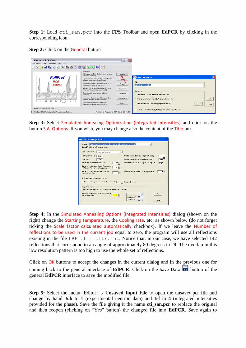
Step 1: Load cti_san.pcr into the FPS Toolbar and open EdPCR by clicking in the

corresponding icon.

Step 2: Click on the General button

Step 3: Select Simulated Annealing Optimization (Integrated Intensities) and click on the

button S.A. Options. If you wish, you may change also the content of the Title box.

Step 4: In the Simulated Annealing Options (Integrated Intensities) dialog (shown on the

right) change the Starting Temperature, the Cooling rate, etc, as shown below (do not forget

ticking the Scale factor calculated automatically checkbox). If we leave the Number of reflections to be used in the current job equal to zero, the program will use all reflections

existing in the file LBF_cti1_cltr.int. Notice that, in our case, we have selected 142

reflections that correspond to an angle of approximately 80 degrees in 2. The overlap in this

low resolution pattern is too high to use the whole set of reflections.

Click on OK buttons to accept the changes in the current dialog and in the previous one for

coming back to the general interface of EdPCR. Click on the Save Data button of the

general EdPCR interface to save the modified file.

Step 5: Select the menu: Editor Unsaved Input File to open the unsaved.pcr file and

change by hand Job to 1 (experimental neutron data) and Irf to 4 (integrated intensities

provided for the phase). Save the file giving it the name cti_san.pcr to replace the original

and then reopen (clicking on “Yes” button) the changed file into EdPCR. Save again to

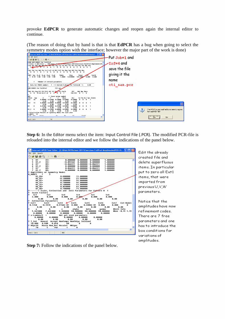
provoke EdPCR to generate automatic changes and reopen again the internal editor to

continue.

(The reason of doing that by hand is that is that EdPCR has a bug when going to select the

symmetry modes option with the interface; however the major part of the work is done)

Step 6: In the Editor menu select the item: Input Control File (.PCR). The modified PCR-file is

reloaded into the internal editor and we follow the indications of the panel below.

Step 7: Follow the indications of the panel below.

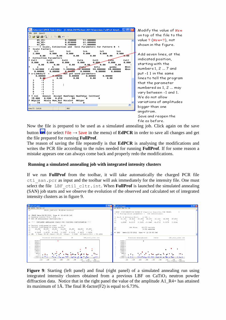
Now the file is prepared to be used as a simulated annealing job. Click again on the save

button (or select File → Save in the menu) of EdPCR in order to save all changes and get

the file prepared for running FullProf.

The reason of saving the file repeatedly is that EdPCR is analysing the modifications and

writes the PCR file according to the rules needed for running FullProf. If for some reason a

mistake appears one can always come back and properly redo the modifications.

Running a simulated annealing job with integrated intensity clusters

If we run FullProf from the toolbar, it will take automatically the charged PCR file

cti_san.pcr as input and the toolbar will ask immediately for the intensity file. One must

select the file LBF_cti1_cltr.int. When FullProf is launched the simulated annealing

(SAN) job starts and we observe the evolution of the observed and calculated set of integrated

intensity clusters as in figure 9.

Figure 9: Starting (left panel) and final (right panel) of a simulated annealing run using

integrated intensity clusters obtained from a previous LBF on CaTiO3 neutron powder

diffraction data. Notice that in the right panel the value of the amplitude A1_R4+ has attained

its maximum of 1Å. The final R-factor(F2) is equal to 6.73%.

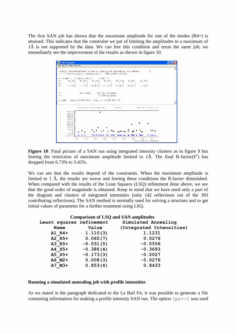
The first SAN job has shown that the maximum amplitude for one of the modes (R4+) is

attained. This indicates that the constraint we put of limiting the amplitudes to a maximum of

1Å is not supported by the data. We can free this condition and rerun the same job; we

immediately see the improvement of the results as shown in figure 10.

Figure 10: Final picture of a SAN run using integrated intensity clusters as in figure 9 but

freeing the restriction of maximum amplitude limited to 1Å. The final R-factor(F2) has

dropped from 6.73% to 3.45%.

We can see that the results depend of the constraints. When the maximum amplitude is

limited to 1 Å, the results are worse and freeing these conditions the R-factor diminished.

When compared with the results of the Least Squares (LSQ) refinement done above, we see

that the good order of magnitude is obtained. Keep in mind that we have used only a part of

the diagram and clusters of integrated intensities (only 142 reflections out of the 393

contributing reflections). The SAN method is normally used for solving a structure and to get

initial values of parameter for a further treatment using LSQ.

Comparison of LSQ and SAN amplitudes Least squares refinement Simulated Annealing

Name Value (Integrated Intensities)

A1_R4+ 1.110(3) 1.1231

A2_R5+ 0.065(7) 0.0276

A3_R5+ -0.031(5) -0.0556

A4_X5+ -0.386(4) -0.3693

A5_X5+ -0.173(3) -0.2027

A6_M2+ 0.008(3) -0.0276

A7_M3+ 0.853(4) 0.8433

Running a simulated annealing job with profile intensities

As we stated in the paragraph dedicated to the Le Bail Fit, it was possible to generate a file

containing information for making a profile intensity SAN run. The option Ipr=-1 was used

for output the file LBF_cti.spr. If we copy the file cti_san.pcr into the file

cti_san_spr.pcr we can transform it easily to run SAN jobs using profile intensities.

We need only to change the value of Ipr to -1. We need also to rename the file

LBF_cti.spr to cti_san_spr.spr in order to run FullProf with the PCR file named

as cti_san_spr.pcr

The program will still need the file of integrated intensities LBF_cti1_cltr.int but it

uses the file just for getting the Miller indices of the reflections.

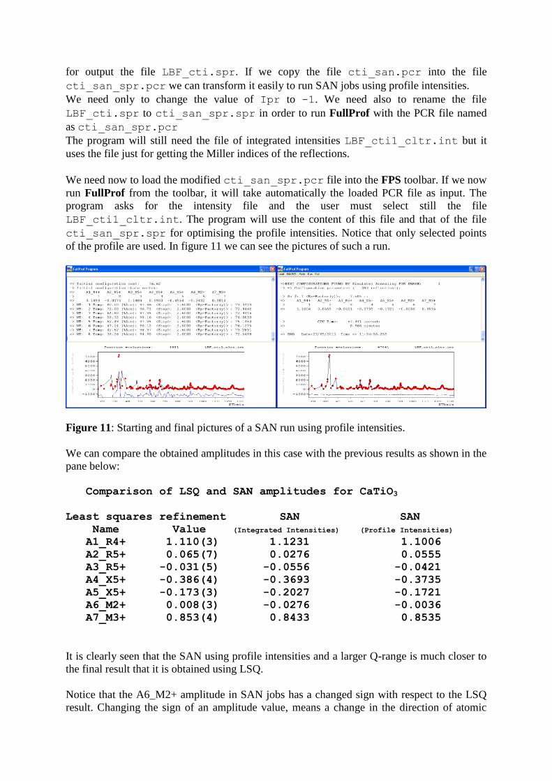
We need now to load the modified cti_san_spr.pcr file into the FPS toolbar. If we now

run FullProf from the toolbar, it will take automatically the loaded PCR file as input. The

program asks for the intensity file and the user must select still the file

LBF_cti1_cltr.int. The program will use the content of this file and that of the file

cti_san_spr.spr for optimising the profile intensities. Notice that only selected points

of the profile are used. In figure 11 we can see the pictures of such a run.

Figure 11: Starting and final pictures of a SAN run using profile intensities.

We can compare the obtained amplitudes in this case with the previous results as shown in the

pane below:

Comparison of LSQ and SAN amplitudes for CaTiO3

Least squares refinement SAN SAN

Name Value (Integrated Intensities) (Profile Intensities)

A1_R4+ 1.110(3) 1.1231 1.1006

A2_R5+ 0.065(7) 0.0276 0.0555

A3_R5+ -0.031(5) -0.0556 -0.0421

A4_X5+ -0.386(4) -0.3693 -0.3735

A5_X5+ -0.173(3) -0.2027 -0.1721

A6_M2+ 0.008(3) -0.0276 -0.0036

A7_M3+ 0.853(4) 0.8433 0.8535

It is clearly seen that the SAN using profile intensities and a larger Q-range is much closer to

the final result that it is obtained using LSQ.

Notice that the A6_M2+ amplitude in SAN jobs has a changed sign with respect to the LSQ

result. Changing the sign of an amplitude value, means a change in the direction of atomic

displacements related to the mode concerned with this amplitude. In some cases this gives rise

to another structure that may correspond to a local minimum. In our case the concerned

amplitude is very small. The sign of the amplitudes is an issue that should be studied in detail

because both LSQ and SAN may be trapped in a local minimum.

The case of LaMnO3

We provide also neutron powder diffraction data corresponding to LaMnO3, another

perovskite with the same structure as that of CaTiO3. The data were taken on the

diffractometer 3T2 at LLB. The input file LaMnO3.dat (the format of the file corresponds

to Ins=6) was collected with a wavelength =1.229Å, the unit cell parameters in this case

are a= 5.747Å, b=7.693Å and c=5.536Å. The UVW parameters of 3T2 are approximately:

U=0.177, V=-0.199 and W= 0.0925. With this information, the user should be able to redo the

same process described for CaTiO3 in the above paragraphs. In practice the template

generated by AMPLIMODES has the proper values of the UVW parameters; however the unit

cell must be adapted to be closer to the real cell. Let us just give the final results we obtained

after refining the data of LaMnO3 by LSQ as extracted from the file LaMnO3ref.sum.

=> Amplitudes of symmetry modes

Name Value Sigma

A1_R4+ 1.194835 0.002608

A2_R5+ 0.083992 0.002215

A3_R5+ -0.019105 0.002860

A4_X5+ -0.545605 0.001912

A5_X5+ -0.141112 0.002648

A6_M2+ -0.363314 0.002912

A7_M3+ 0.904234 0.002523

=======================================================================

=== FINAL ATOMS POSITIONS CALCULATED FROM SYMMETRY MODES FOR PHASE: 1

=======================================================================



=> Global Amplitude of Representation X5+ : 0.5636(20)

=> Global Amplitude of Representation M2+ : 0.363(3)

=> Global Amplitude of Representation M3+ : 0.904(3)

X Y Z B-iso Occ

Atom La1 -0.04895(17) 0.25000 0.50754(20) 0.355(15) 0.50000

Atom Mn1 0.00000 0.00000 0.00000 0.24(3) 0.50000

Atom O1 0.30686(17) -0.03851(12) 0.22573(17) 0.434(16) 1.00000

Atom O1_2 0.0127(2) 0.25000 0.0746(2) 0.51(2) 0.50000

Notice that the data taken on LaMnO3 at 3T2 are of higher resolution than those of CaTiO3 so

that the standard deviations are smaller.

Both structures are quite similar concerning the most important rotational modes R4+ and

M3+. The main difference comes from the value of the amplitude corresponding to the Jahn-

Teller mode M2+.

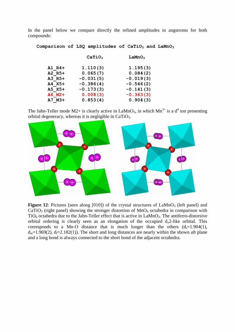
In the panel below we compare directly the refined amplitudes in angstroms for both

compounds:

Comparison of LSQ amplitudes of CaTiO3 and LaMnO3

CaTiO3 LaMnO3

A1_R4+ 1.110(3) 1.195(3)

A2_R5+ 0.065(7) 0.084(2)

A3_R5+ -0.031(5) -0.019(3)

A4_X5+ -0.386(4) -0.546(2)

A5_X5+ -0.173(3) -0.141(3)

A6_M2+ 0.008(3) -0.363(3)

A7_M3+ 0.853(4) 0.904(3)

The Jahn-Teller mode M2+ is clearly active in LaMnO3, in which Mn3+

is a d4 ion presenting

orbital degeneracy, whereas it is negligible in CaTiO3.

Figure 12: Pictures (seen along [010]) of the crystal structures of LaMnO3 (left panel) and

CaTiO3 (right panel) showing the stronger distortion of MnO6 octahedra in comparison with

TiO6 octahedra due to the Jahn-Teller effect that is active in LaMnO3. The antiferro-distorsive

orbital ordering is clearly seen as an elongation of the occupied dz2-like orbital. This

corresponds to a Mn-O distance that is much longer than the others (ds=1.904(1),

dm=1.969(2), dl=2.182(1)). The short and long distances are nearly within the shown ab plane

and a long bond is always connected to the short bond of the adjacent octahedra.

Documents

FullProf Tutorial - Bilbao Crystallographic Server · 2019-01-10 · splitting of the Wyckoff orbits in H. ( , ) ( , ) ( , ) The indices and m label all possible distinct allowed