Embed Size (px)
Citation preview
2. FUNDAMENTAL MEASURES OF DISEASE OCCURRENCE AND ASSOCIATlON
2.1 Measures of disease occurrence
2.2 Age- and time-specific incidence rates
2.3 Cumulative incidence rates
2.4 Models of disease association
2.5 Empirical behaviour of the relative risk
2.6 Effects of combined exposures
2.7 Logical properties of the relative risk
2.8 Estimation of the relative risk from case-control studies - basic concepts
2.9 Attributable risk and related measures
CHAPTER I1
FUNDAMENTAL MEASURES OF DISEASE OCCURRENCE AND ASSOCIATION
The occurrence of particular cancers varies remarkably according to a wide range of factors, including age, sex, calendar time, geography and ethnicity. Etiological studies attempt to explain such variation by relating disease occurrence to genetic markers, or to exposure to particular environmental agents, which may have a similar variation in time and space. The cancer epidemiologist studies how the disease depends on the constellation of risk factors acting on the population and uses this information to determine the best measures for prevention and control. This process requires a quantitative measure of exposure, as well as one of disease occurrence, and some method of associating the two.
In this chapter we introduce the fundamental concepts of disease incidence rates, cumulative incidence, and risk. These will allow us to make a precise comparison of disease occurrence in different populations. Relative risk is defined and shown to have both empirical and logical advantages as a measure of disease/risk factor association, especially in connection with case-control studies. The close connection between cohort and case-control studies is emphasised throughout.
2.1 Measures of disease occurrence
Two measures of disease frequency, incidence and prevalence, are commonly intro- duced in textbooks on epidemiology. Point prevalence is the proportion of a defined population affected by the disease in question at a specified point in time. The numerator of the proportion comprises all those who have the disease at that instant, regardless of whether it was contracted recently or long ago. Thus, diseases of long duration tend to have a higher prevalence than short-term illnesses, even if the total numbers of affected individuals are about equal.
Incidence refers to new cases of disease occurring among previously unaffected individuals. This is a more appropriate measure for etiological studies of cancer and other chronic illnesses, wherein one attempts to relate disease occurrence to genetic and environmental factors in a framework of causation. The duration of survival of patients with a given disease, and hence its prevalence, may be influenced by treat- ment and other factors which come into play after onset. Early reports of an associa- tion between the antigen HL-A2 and risk for acute leukaemia (Rogentine et al., 1972), for example, were later corrected when it was shown that the effect was o n survival rather than- on incidence (Rogentine et al., 1973). Since causal factors necessarily
MEASURES OF DISEASE 43
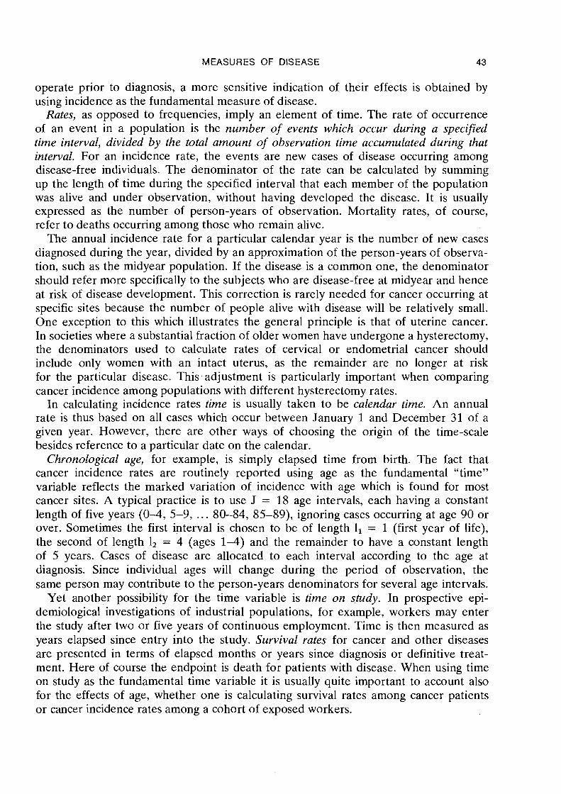
operate prior to diagnosis, a more sensitive indication of their effects is obtained by using incidence as the fundamental measure of disease.
Rates, as opposed to frequencies, imply an element of time. The rate of occurrence of an event in a population is the number of events which occur during a specified time interval, divided by the total amount of observation time accumulated during that interval. For an incidence rate, the events are new cases of disease occurring among disease-free individuals. The denominator of the rate can be calculated by summing up the length of time during the specified interval that each member of the population was alive and under observation, without having developed the disease. It is usually expressed as the number of person-years of observation. Mortality rates, of course, refer to deaths occurring among those who remain alive.
The annual incidence rate for a particular calendar year is the number of new cases diagnosed during the year, divided by an approximation of the person-years of observa- tion, such as the midyear population. If the disease is a common one, the denominator should refer more specifically to the subjects who are disease-free at midyear and hence at risk of disease development. This correction is rarely needed for cancer occurring at specific sites because the number of people alive with disease will be relatively small. One exception to this which illustrates the general principle is that of uterine cancer. In societies where a substantial fraction of older women have undergone a hysterectomy, the denominators used to calculate rates of cervical or endometrial cancer should include only women with an intact uterus, as the remainder are no longer at risk for the particular disease. This adjustment is particularly important when comparing cancer incidence among populations with different hysterectomy rates.
In calculating incidence rates time is usually taken to be calendar time. An annual rate is thus based on all cases which occur between January 1 and December 31 of a given year. However, there are other ways of choosing the origin of the time-scale besides reference to a particular date on the calendar.
Chronological age, for example, is simply elapsed time from birth. The fact that cancer incidence rates are routinely reported using age as the fundamental "time" variable reflects the marked variation of incidence with age which is found for most cancer sites. A typical practice is to use J = 18 age intervals, each having a constant length of five years (0-4, 5-9, . . . 80-84, 85-89), ignoring cases occurring at age 90 or over. Sometimes the first interval is chosen to be of length l1 = 1 (first year of life), the second of length 1, = 4 (ages 1-4) and the remainder to have a constant length of 5 years. Cases of disease are allocated to each interval according to the age at diagnosis. Since individual ages will change during the period of observation, the same person may contribute to the person-years denominators for several age intervals.
Yet another possibility for the time variable is time on study. In prospective epi- demiological investigations of industrial populations, for example, workers may enter the study after two or five years of continuous employment. Time is then measured as years elapsed since entry into the study. Survival rates for cancer and other diseases are presented in terms of elapsed months or years since diagnosis or definitive treat- ment. Here of course the endpoint is death for patients with disease. When using time on study as the fundamental time variable it is usually quite important to account also for the effects of age, whether one is calculating survival rates among cancer patients or cancer incidence rates among a cohort of exposed workers.
44 BRESLOW & DAY
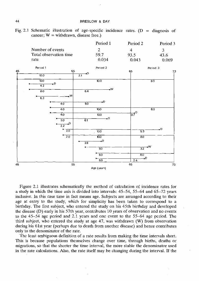
Fig. 2.1 Schematic illustration of age-specific incidence rates. (D = diagnosis of cancer; W = withdrawn, disease free.)
Period 1 Period 2 Period 3
Number of events 2 4 3 Total observation time 59.7 93.5 43.6 rate 0.034 0.04 3 0.069
Figure 2.1 illustrates schematically the method of calculation of incidence rates for a study in which the time axis is divided into intervals: 45-54, 55-64 and 65-72 years inclusive. In this case time in fact means age. Subjects are arranged according to their age at entry to the study, which for simplicity has been taken to correspond to a birthday. The first subject, who entered the study on his 45th birthday and developed the disease (D) early in his 57th year, contributes 10 years of observation and no events to the 45-54 age period and 2.1 years and one event to the 55-64 age period. The third subject, who entered the study at age 47, was withdrawn (W) from observation during his 61st year (perhaps due to death from another disease) and hence contributes only to the denominator of the rate.
The least ambiguous definition of a rate results from making the time intervals short. This is because populations themselves change over time, through births, deaths or migrations, so that the shorter the time interval, the more stable the denominator used in the rate calculations. Also, the rate itself may be changing during the interval. If the
Period 1 Period 2 Period 3 45 5
1 ,
10.0 I
10.0 . D 4 2
l
8.0 . .W 6.3
* 4.0 . 4.0
4.0
3.0 -D
2.2
2.0 l
2.0
45 Age (years)
5 mD
2.1
10.0
r W 6.4
. D 5.0
10.0
10.0 OD
6.1
10.0
10.0 . .D 3.9 .
8.0 b
6.0 . 6.0
55 65
65 7
8.0
8.0 . D 0.7
. D 5.3
8.0
W 3.2
8.0 .D
2.4
73
3
MEASURES OF DISEASE 4 5
change is rapid it makes sense to consider short intervals-so that information about the magnitude of the change is not lost; but if the intervals are too short only a few events will be observed in each one. The instability of the denominator must be balanced against statistical fluctuations in the numerator when deciding upon an appropriate time interval for calculation of a reasonably stable rate.
If an infinite population were available, so that statistical stability was not in question, one could consider making the time intervals used for the rate calculation infinitesimal. As the length of each interval approaches zero, one obtains in the limit an instantaneo~rs rate i,(t) defined for each instant t of time. This concept has proved very useful in actuarial science, where, with the event in question being death, i.(t) represents the force of mortality. In the literature of reliability analysis, where the event is failure of some system component, L(t) is referred to as the hazard rate. When the endpoint is diagnosis of disease in a previously disease-free individual, we can refer to the instan- taneous incidence rate as the force of morbidity.
The method of calculation of the estimated rate will depend upon the type of data available for analysis. It is perhaps simplest in .the case of a longitudinal follow-up study of a fixed population of individuals, for example: mice treated with some carcinogen who are followed from birth for appearance of tumours; cancer patients followed from time of initial treatment until relapse or death; or employees of a given industry or plant who are followed from date of employment until diagnosis of disease. A com- mon method of estimating incidence or mortality rates with such data is to divide the time axis into J intervals having lengths lj and midpoints tj. Denote by nj the number of subjects out of the original population of no who are still under observation and at risk at tj. Let dj be the number of events- (diagnoses or deaths) observed during the jth interval. Then the incidence at time tj may be estimated by
that is; by the number of events observed per subject, per unit time in the population at risk during the interval. Of course the denominator in equation (2.1) is only an approximation to the total observation time accumulated during the interval, which should be used if available.
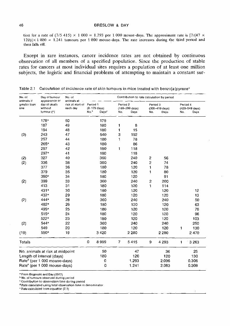
Example: An example of the calculation of incidence rates from follow-up studies is given. in Table 2.1 which lists the days until appearance of skin tumours for a group of 50 albino mice treated with benzo[a]- pyrene (Bogovski & Day, 1977). For the purpose of illustration, the duration of the study has been divided into four periods of unequal length: 0-179 days, 180-299 days, 300-419 days and 420-549 days. These are rather wider than is generally desirable because of limited data. Nineteen of the animals survived the entire 550 days without developing skin tumours, and are listed together at the bottom of the table. The contribution of each animal to the number of tumours and total observation time for each period are shown. Thus, the mouse developing tumour at 377 days contributes 0 tumours and 180 days observation to Period 1, 0 tumours and 120 days observation to Period 2, and 1 tumour and 78 days observation to Period 3.
Tumour incidence rates shown at the bottom of Table 2.1 were calculated in two ways. The first used the actual total observation time in each period, while the second used the approximation to this based on the number of animals alive at the midpoint (equation 2.1). Thus the incidence rate for Period 1 is 0 as no tumours were observed. For Period 2, 7 tumours were seen during 5 415 mouse-days of observa-
46 BRESLOW & DAY
tion for a rate of (7/5 415) x 1 000 = 1.293 per 1 0 0 0 mouse-days. The approximate rate is [7/(47 x 120)) x 1 000 = 1.241 tumours per 1 000 mouse-days. The rate increases during the third period and then falls off.
Except in rare instances, cancer incidence rates are not obtained by continuous observation of all members of a specified population. Since the production of stable rates for cancers at most individual sites requires a population of at least one million subjects, the logistic and financial problems of attempting to maintain a constant sur-
Table 2.1 Calculation of incidence rate of skin tumours in mice treated with benzola Ipyrene"
No. of Day of tumour No. of Contribution to rate calculation by period animals if appearance or animals at greater than day of death risk at start of Period 1 Period 2 Period 3 Period 4 one without each day (0-179 days) (1 80-299 days) (30011 19 days) (420-549 days)
tumour (*) N o . V a y s c No. Days No. Days No. Days
Totals 0 8 999 7 5 4 1 5
No. animals at risk at midpoint 50 47 Length of interval (days) 180 120 Rated (per 1 000 mouse-days) 0 1.293 Ratee (per 1 000 mouse-days) 0 1.241
" From Bogovski and Day (1977) No. of tumours observed during period
'Contribution to obse~a t ion time during period Rate calculated using total observation time in denominator Rate calculated from equation (2.1)
MEASURES OF DISEASE 4 7
veillance system are usually prohibitive. The information typically available to a cancer registry for calculation of rates includes the cancer cases, classified by sex, age and year of diagnosis, together with estimates of the population denominators obtained from the census department. How good the estimated denominators are depends on the frequency and accuracy of the census in each locality.
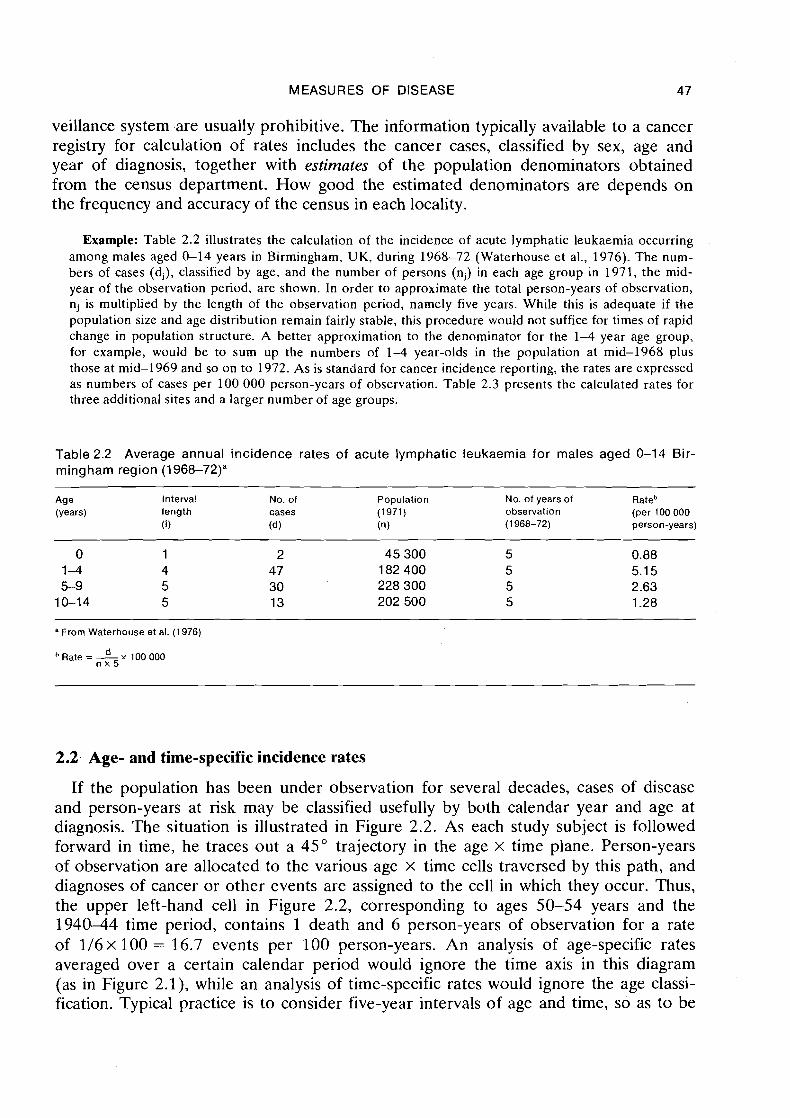
Example: Table 2.2 illustrates the calculation of the incidence of acute lymphatic leukaemia occurring among males aged 0-14 years in Birmingham, UK, during 1968-72 (Waterhouse e t al., 1976). The num- bers of cases (dj), classified by age, and the number of persons (nj) in each age group in 1971, the mid- year of the observation period, are shown. In order to approximate the total person-years of observation, nj is multiplied by the length of the observation period, namely five years. While this is adequate if the population size and age distribution remain fairly stable, this procedure would not suffice for times of rapid change in population structure. A better approximation to the denominator for the 1-4 year age group, for example, would be to sum up the numbers of 1 - 4 year-olds in the population at mid-1968 plus those at mid-1 969 and so on to 1972. As is standard for cancer incidence reporting, the rates are expressed as numbers of cases per 100 000 person-years of observation. Table 2.3 presents the calculated rates for three additional sites and a larger number of age groups.
Table 2.2 Average annual incidence rates of acute lymphatic leukaemia for males aged 0-14 Bir- mingham region (1968-72)"
Age Interval No. of Population No. of years of Rateh (Years) length cases (1971) observation (per 100 000
(1) (d) (n) (1 968-72) person-years)
' From Waterhouse et al. (1976)
Rate = d v 100 000 n x 5
2.2 Age- and time-specific incidence rates
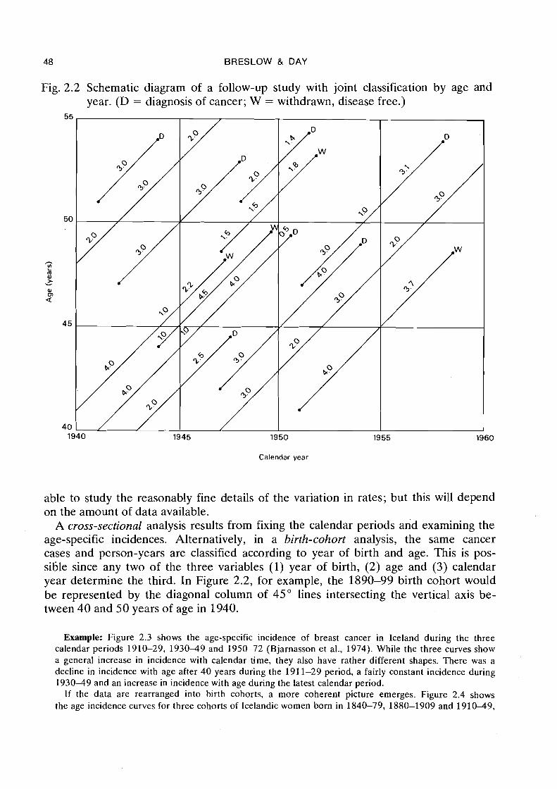
If the population has been under observation for several decades, cases of disease and person-years at risk may be classified usefully by both calendar year and age at diagnosis. The situation is illustrated in Figure 2.2. As each study subject is followed forward in time, he traces out a 45" trajectory in the age x time plane. Person-years of observation are allocated to the various age x time cells traversed by this path, and diagnoses of cancer or other events are assigned to the cell in which they occur. Thus, the upper left-hand cell in Figure 2.2, corresponding to ages 50-54 years and the 194044 time period, contains 1 death and 6 person-years of observation for a rate of 1/6x 100 = 16.7 events per 100 person-years. An analysis of age-specific rates averaged over a certain calendar period would ignore the time axis in this diagram (as in Figure 2.1), while an analysis of time-specific rates would ignore the age classi- fication. Typical practice is to consider five-year intervals of age and time, so as to be
48 BRESLOW & DAY
Fig. 2.2 Schematic diagram of a follow-up study with joint classification by age and year. (D = diagnosis of cancer; W = withdrawn, disease free.)
able to study the reasonably fine details of the variation in rates; but this will depend on the amount of data available.
A cross-sectional analysis results from fixing the calendar periods and examining the age-specific incidences. Alternatively, in a birth-cohort analysis, the same cancer cases and person-years are classified according to year of birth and age. This is pos- sible since any two of the three variables (1) year of birth, (2) age and (3) calendar year determine the third. In Figure 2.2, for example, the 1890-99 birth cohort would be represented by the diagonal column of 45" lines intersecting the vertical axis be- tween 40 and 50 years of age in 1940.
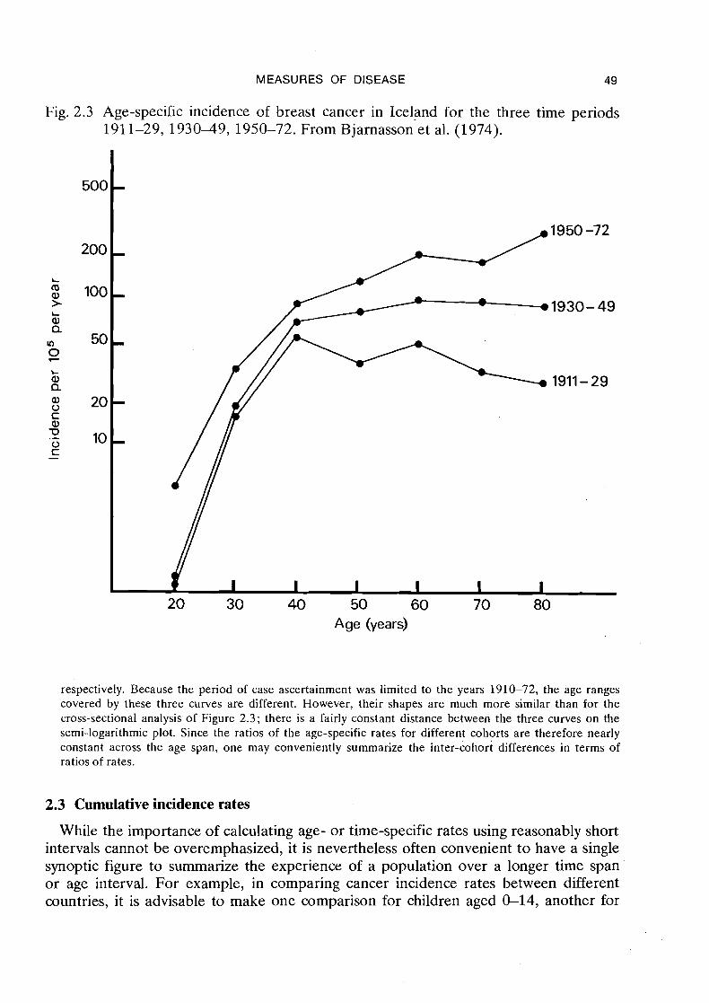
Example: Figure 2.3 shows the age-specific incidence of breast cancer in Iceland during the three calendar periods 1910-29, 1930-49 and 1950-72 (Bjarnasson et al., 1974). While the three curves show a general increase in incidence with calendar time, they also have rather different shapes. There was a decline in incidence with age after 40 years during the 191 1-29 period, a fairly constant incidence during 1930-49 and an increase in incidence with age during the latest calendar period.
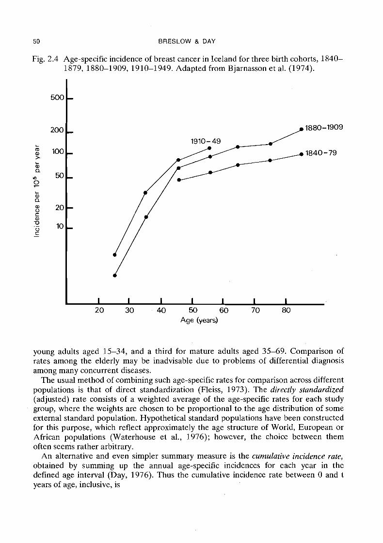
If the data are rearranged into birth cohorts, a more coherent picture emerges. Figure 2.4 shows the age incidence curves for three cohorts of Icelandic women born in 1840-79, 1880-1909 and 1910-49,
MEASURES OF DISEASE 49
Fig. 2.3 Age-specific incidence of breast cancer in Iceland for the three time periods 1911-29, 193049, 1950-72. From Bjarnasson et al. (1974).
Age (years)
respectively. Because the period of case ascertainment was limited to the years 1910-72, the age ranges covered by these three curves are different. However, their shapes are much more similar than for the cross-sectional analysis of Figure 2.3; there is a fairly constant distance between the three curves on the semi-logarithmic plot. Since the ratios of the age-specific rates for different cohorts are therefore nearly constant across the age span, one may conveniently summarize the inter-cohort differences in terms of ratios of rates.
2.3 Cumulative incidence rates
While the importance of calculating age- or time-specific rates using reasonably short intervals cannot be overemphasized, it is nevertheless often convenient to have a single synoptic figure to summarize the experience of a population over a longer time span or age interval. For example, in comparing cancer incidence rates between different countries, it is advisable to make one comparison for children aged G14, another for
50 BRESLOW & DAY
Fig. 2.4 Age-specific incidence of breast cancer in Iceland for three birth cohorts, 1840- 1879, 1880-1909, 1910-1 949. Adapted from Bjarnasson et al. (1974).
Age (years)
young adults aged 15-34, and a third for mature adults aged 35-69. Comparison of rates among the elderly may be inadvisable due to problems of differential diagnosis among many concurrent diseases.
The usual method of combining such age-specific rates for comparison across different populations is that of direct standardization (Fleiss, 1973). The directly standardized (adjusted) rate consists of a weighted average of the age-specific rates for each study group, where the weights are chosen to be proportional to the age distribution of some external standard population. Hypothetical standard populations have been constructed for this purpose, which reflect approximately the age structure of World, European or African populations (Waterhouse et al., 1976); however, the choice between them often seems rather arbitrary.
An alternative and even simpler summary measure is the cumulative incidence rate, obtained by summing up the annual age-specific incidences for each year in the defined age interval (Day, 1976). Thus the cumulative incidence rate between 0 and t years of age, inclusive, is
MEASURES OF DISEASE
t
A (t) = 2 l ( n ) n=O
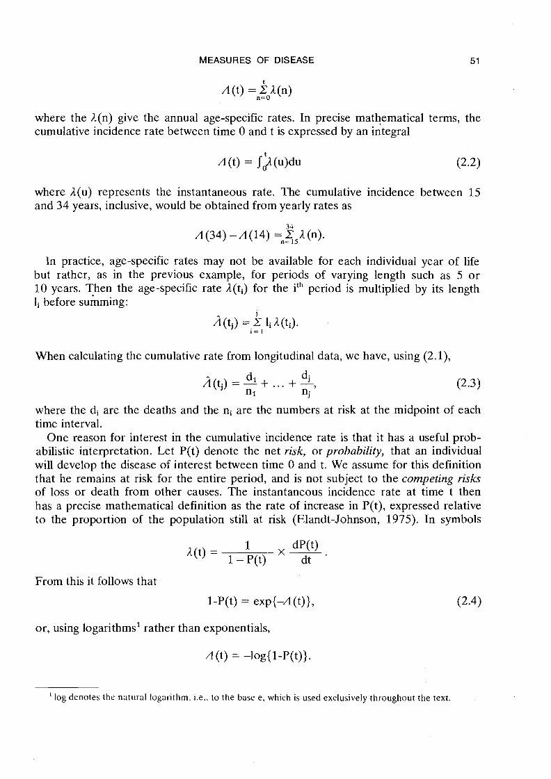
where the l (n ) give the annual age-specific rates. In precise mathematical terms, the cumulative incidence rate between time 0 and t is expressed by an integral
where l (u ) represents the instantaneous rate. The cumulative incidence between 15 and 34 years, inclusive, would be obtained from yearly rates as
In practice, age-specific rates may not be available for each individual year of life but rather, as in the previous example, for periods of varying length such as 5 or 10 years. Then the age-specific rate l ( t i ) for the ith period is multiplied by its length li before summing:
When calculating the cumulative rate from longitudinal data, we have, using (2.1),
where the di are the deaths and the ni are the numbers at risk at the midpoint of each time interval.
One reason for interest in the cumulative incidence rate is that it has a useful prob- abilistic interpretation. Let P(t) denote the net risk, or probability, that an individual will develop the disease of interest between time 0 and t. We assume for this definition that he remains at risk for the entire period, and is not subject to the competing risks of loss or death from other causes. The instantaneous incidence rate at time t then has a precise mathematical definition as the rate of increase in P(t), expressed relative to the proportion of the population still at risk (Elandt-Johnson, 1975). In symbols
From this it follows that
1 -P(t) = exp{-A (t)),
or, using logarithms' rather than exponentials,
A (t) = -log{l-P(t)).
' log denotes the n a t ~ ~ r a l logarithm. i .e . , to the base e . which is used exclusively throughout the text.
5 2 BRESLOW & DAY
These equations tell us that when the disease is rare or the time period short, so that the cumulative incidence or mortality is small, then the probability of disease occur- rence is well approximated by the cumulative incidence
P(t) -A (t).
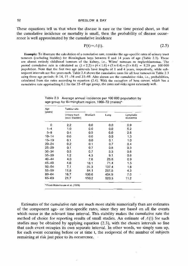
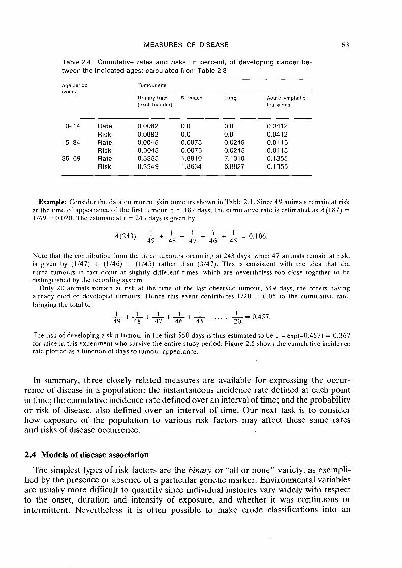
Example: T o illustrate the calculation of a cumulative rate, consider the age-specific rates of urinary tract tumours (excluding bladder) for Birmingham boys between 0 and 14 years of age (Table 2.3). These are almost entirely childhood tumours of the kidney, i.e., Wilms' tumours or nephroblastomas. The period cumulative rate is calculated as (1 x 2.2) + (4 X 1.0) + (5 x 0.4) + (5 x 0.0) = 8.20 per 100 000 population. Note that the first two age intervals have lengths of 1 and 4 years, respectively, while sub- sequent intervals are five years each. Table 2.4 shows the cumulative rates for all four tumours in Table 2.3 using three age periods: 0-14, 15 -34 and 35-69. Also shown are the cumulative risks, i.e., probabilitiesj calculated from the rates according to equation (2.4). With the excepfion of lung cancer, which has a cumulative rate approaching 0.1 for the 35-69 age group, the rates and risks agree extremely well.
Table 2.3 Average annual incidence per 100 000 population by age group for Birmingham region, 1968-72 (males)"
Age Tumour site (years)
Urinary tract ~ t o ~ a c h Lung Lymphatic (excl. bladder) leukaemia
"From Waterhouse et al. (1976)
Estimates of the cumulative rate are much more stable numerically than are estimates of the component age- or time-specific rates, since they are based on all the events which occur in the relevant time interval. This stability makes the cumulative rate the method of choice for reporting results of small studies. An estimate of A(t) for such studies may be obtained by applying equation (2.3), with the chosen intervals so fine that each event occupies its own separate interval. In other words, we simply sum up, for each event occurring before or at time t, the reciprocal of the number of subjects remaining at risk just prior to its occurrence.
MEASURES OF DISEASE
Table 2.4 Cumulative rates and risks, in percent, of developing cancer be- tween the indicated ages: calculated from Table 2.3
Age period
(Years)
Tumour site
Urinary tract Stomach Lung Acute lymphatic (excl. bladder) leukaem~a
0-1 4 Rate 0.0082 0.0 0.0 0.041 2 Risk 0.0082 0.0 0.0 0.0412
15-34 Rate 0.0045 0.0075 0.0245 0.01 15 Risk 0.0045 0.0075 0.0245 0.01 15
35-69 Rate 0.3355 1.8810 7.131 0 0.1355 Risk 0.3349 1.8634 6.8827 0.1 355
Example: Consider the data on murine skin tumours shown in Table 2.1. Since 49 animals remain at risk at the time of appearance of the first tumour, t = 187 days, the cumulative rate is estimated as A(187) =
1/49 = 0.020. The estimate at t = 243 days is given by
Note that, the contribution from the three tumours occurring at 243 days, when 47 animals remain at risk, is given by (1/47) + (1/46) + (1/45) rather than (3/47). This is consistent with the idea that the three tumours in fact occur at slightly different times. which are nevertheless too close together to be distinguished by the recording system.
Only 20 animals remain at risk at the time of the last observed tumour, 549 days, the others having already died or developed tumours. Hence this event contributes 1/20 = 0.05 to the cumulative rate. bringing the total to
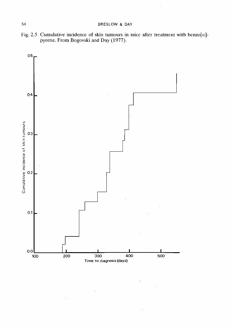
The risk of developing a skin tumour in the first 550 days is thus estimated to be 1 - exp(-0.457) = 0.367 for mice in this experiment who survive the entire study period. Figure 2.5 shows the cumulative incidence rate plotted as a function of days to tumour appearance.
In summary, three closely related measures are available for expressing the occur- rence of disease in a population: the instantaneous incidence rate defined at each point in time; the cumulative incidence rate defined over an interval of time; and the probability o r risk of disease, also defined over an interval of time. Our next task is to consider how exposure of the population to various risk factors may affect these same rates and risks of disease occurrence.
2.4 Models of disease association
The simplest types of risk factors are the binary or "all or none" variety, as exempli- fied by the presence or absence of a particular genetic marker. Environmental variables are usually more difficult to quantify since individual histories vary widely with respect to the onset, duration and intensity of exposure, and whether it was continuous or intermittent. Nevertheless it is often possible to make crude classifications into an
54 BRESLOW & DAY
Fig. 2.5 Cumulative incidence of skin tumours in mice after treatment with benzo[a]- pyrene. From Bogovski and Day (1977).
100 200 300 400 500 Time to diagnosis (days)
MEASURES OF DISEASE 55
exposed versus a non-exposed group, for example by comparing confirmed cigarette smokers with non-smokers, or lifelong urban with lifelong rural residents. In order to introduce the concept of risk factor/disease association, we suppose here that the population has been divided into two such subgroups, one exposed to the risk factor in question and the other not exposed.
As shown in the earlier examples, incidence rates may vary widely within the popula- tion according to such factors as age, sex and calendar year of observation. Thus whatever measure is used to compare incidence rates in the exposed versus non- exposed subgroups, this too is likely to vary by age, sex and time. What is clearly desired in this situation is a measure of association which is as stable as possible over the various subdivisions of the population; the more nearly constant it is, the greater is the justification for expressing the effect of exposure in a single summary number; the more it varies, the greater is the necessity to describe how the effect of exposure is modified by demographic or other relevant factors on which information is available.
Suppose that the population has been divided into I strata on the basis of age, sex, calendar period of observation, or combinations of these and other features. Denote by ,Ili the incidence rate of disease in the ith stratum for the exposed subgroup and by ,Ioi the rate for the non-exposed subgroup in that stratum. The first measure of associa- tion we consider is the excess risk of disease, defined as the difference between the stratum-specific incidences
Since the measure is defined in terms of incidence rates, rather than risks, it would perhaps be more accurate to refer to it as the excess rate of disease. We follow con- vention by allowing the distinction between risks and rates to be blurred somewhat in discussing measures of association, except when it is critical to the point in question.
The intuitive idea underlying this approach is that cases contributing to the "natural" or background disease incidence rate in the ith stratum are due to the presence of general factors which operate on exposed and non-exposed individuals alike. Cases caused by exposure to the particular agent under investigation are represented in the excess risk bi (Rothman, 1976). If these two causes of disease, the general and the specific, were in some sense operating independently of each other, one might expect the number of excess cases of disease occurring per person-year of observation to reflect only the level of exposure and to be unrelated to the underlying natural risk. Thus the excess risk would be relatively constant from stratum to stratum, apart from random statistical fluctuations.
The idea of a constant excess risk due to the particular exposure may be formally expressed by hypothesizing an additive model for the two dimensional sets of rates. With b representing the additive effect of exposure, the model states
Unfortunately the concept of independence leading to this model is rather simplistic and breaks down when one considers plausible mechanisms for the disease process (Koopman, 1977). Suppose, for example, that a disease was caused in infancy or early childhood but took many years to develop. If the age distribution of the cases
56 BRESLOW & DAY
produced by the specific exposure were the same as that of the spontaneous cases, the differences in age-specific rates would be greater for the ages in which the spontaneous incidence was higher, even if the general and specific exposures had operated inde- pendently of each other early on. Nonetheless (2.7) may be postulated ad hoc, and if it appears to correspond reasonably well to the data, the estimate of b derived from the fitted model may be used as an overall measure of the effect of exposure.
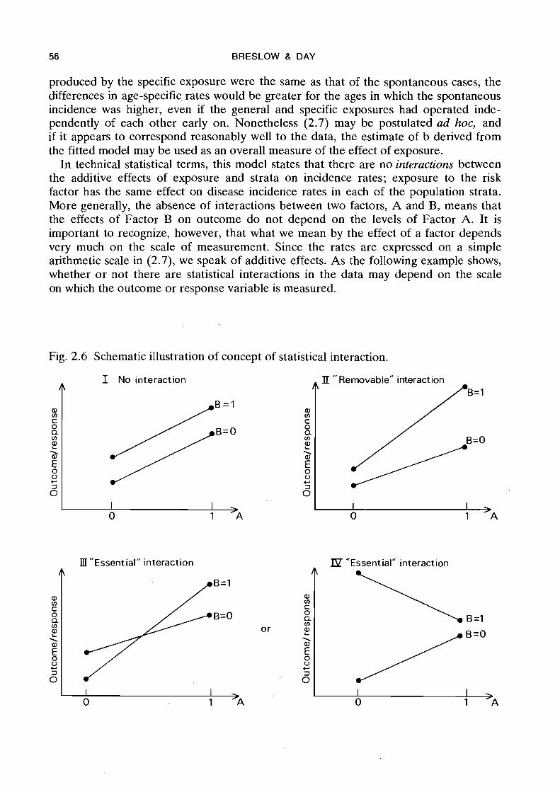
In technical statistical terms, this model states that there are no interactions between the additive effects of exposure and strata on incidence rates; exposure to the risk factor has the same effect on disease incidence rates in each of the population strata. More generally, the absence of interactions between two factors, A and B, means that the effects of Factor B on outcome do not depend on the levels of Factor A. It is important to recognize, however, that what we mean by the effect of a factor depends very much on the scale of measurement. Since the rates are expressed on a simple arithmetic scale in (2.7), we speak of additive effects. As the following example shows, whether o r not there are statistical interactions in the data may depend on the scale on which the outcome or response variable is measured.
Fig. 2.6 Schematic illustration of concept of statistical interaction.
I No interaction
f ' Removable" interact ion
B= l
III "Essential" interaction IP "Essential" interaction
A LBZ1 a, V) c 0 Q V)
2 \ a,
5 0 + 3 0
0 1 )A 0 J______; 1 >A
A B= l
a, V) C
B=O 0 a V)
or ? \
E 0 '2 +
5 I I
MEASURES OF DISEASE 57
Example: Figure 2.6 illustrates the concept of interaction schematically. Conditions for no interaction hold when the two response curves are parallel (Panel I). Note that the definition of interaction is com- pletely symmetric; the diagram shows also that the effect of Factor A is independent of the level of Factor B.
The non-parallel response curves shown in Panel 11 of the figure indicate that Factor B has a greater effect on outcome at level 1 of Factor A than it does at level O. I t is apparent, however, that if the out- come variable were expressed on a different scale, for example a logarithmic or square root scale which tended to bring together the more extreme outcomes, the interaction could be made to disappear. In this sense we may speak of interactions which are "removable" by an appropriate choice of scale.
The situation in Panels 111 and IV, characterized by the response curves either crossing over or having slopes of different signs, allows far no such remedy. In Panel 111 the effect of Factor B is to increase the response at one level of Factor A, and to decrease i t at another, while in Panel 1V it is the sign of the A effect which changes with B. In the present context this would mean that exposure to the risk factor increased the rate of disease for one part of the population and decreased it for another. No change of the outcome scale could alter this essential difference.
While the excess risk is a useful measure in certain contexts, the bulk of this mono- graph deals with another measure of association, for reasons which will be clarified below. This is the relative risk of disease, defined as the ratio of the stratum-specific incidences:
The assumed effect of exposure is to multiply the background rate ,Ioi by the quantity ri. Absence of interactions here leads to a multiplicative model for the rates such that, within the limits of statistical error, these may be expressed as the product of two terms, one representing the underlying natural disease incidence in the stratum and the other representing the relative risk r. More precisely, the model states
where P=log(r). Alternatively, if the incidence rates are expressed on a logarithmic scale, it takes the form
log ,Ili = log ,Ioi +p.
Comparing this with equation (2.7) it is evident that they have precisely the same structure, except for the choice of scale for the outcome measure (incidence rate). In other words, the multiplicative model (2.8) is identical to an additive model in log rates. Such models are called log-linear.
While excess and relative risk are defined here in terms of differences and ratios of stratum-specific incidence rates, analogous measures for the comparison of cumulative rates and risks may be deduced directly from equations (2.2) and (2.4). Suppose, for example, that the two sets of incidence rates have a (constant) difference of 10 cases per 100 000 person-years observation for each year of a particular 15-year time period. Then the difference between the cumulative rates over this same period will be 1 0 x 15 = 150 cases per 100 000 population. On the other hand, if the two sets of rates have a (constant) ratio of 5 for each year, the ratio of the cumulative rates will also equal 5.
58 BRESLOW & DAY
Because there is an exponential term in equation (2.4), the derived relationships between the probabilities, o r risks, for this same time period are not so simple. Let Po(t) denote the net probability that a non-exposed person develops the disease during the time period from 0 to t years, and let Pl(t) denote the analogous quantity for the exposed population. If the corresponding incidence rates satisfy the multiplicative equation ill(u) = rilo(u) for all u between 0 and t, then
This relationship is well approximated by that for the cumulative rates
providing the disease is sufficiently rare, or the time interval sufficiently short, so that both risks and rates remain small. In general, the ratio of disease risks is slightly less extreme, i.e., closer to unity, than is the ratio of the corresponding rates.
We have now introduced the two principal routes by which one may approach the statistical analysis of cancer incidence data: the additive model, where the fundamental measure of association is the excess risk, and the multiplicative model, where the effect of exposure is expressed in relative terms. In order to arrive at a choice between these two, or indeed to decide upon any particular statistical model, several considera- tions are relevant. From a purely empirical viewpoint, the most important properties of a model are simplicity and goodness of fit to the observed data. The aim is to be able to describe the main features of the data as succinctly as possible. Clarity is enhanced by avoiding models with a large number of parameters which must be estimated from the data. If, in one type of model many interaction terms (see 3 6.1) are required to fit the data adequately, whereas with another only a few are required, the latter would generally be preferred.
The empirical properties of a model are not the only criteria. We also need to consider how the results of an analysis are to be interpreted and the meaning that will be attached to the estimated parameters. Excess and relative risks inform us about two quite different aspects of the association between risk factor and disease. Since relative risks for lung cancer among smokers versus non-smokers are generally at least five times those for coronary heart disease, one might be inclined to say that the lung cancer-smoking association is stronger, but this ignores the fact that the differences in rates are generally greater for heart disease. From a public health viewpoint the impact of smoking on mortality from heart disease may be more severe than its effect on lung cancer death rates. This fact has led some authors to advocate exclusive use of the additive measure (Berkson, 1958). Rothman (1976), as noted earlier, has argued that it is the most natural one for measuring interaction.
In spite of these considerations, the relative risk has become the most frequently used measure for associating exposure with disease occurrence in cancer epidemiology, both because of its empirical behaviour and because of several logical properties it possesses. Empirically it provides a summary measure which often requires little quali- fication in terms of the population to which it refers. Logically it facilitates the evalua- tion of the extent to which an observed association is causal. The next two sections
MEASURES OF DISEASE 59
explore these important properties of the relative risk in some detail. We merely point out here that, once having obtained an estimate of the relative risk, it is certainly possible to interpret that estimate in terms of excess risk provided one knows the disease incidence rates for unexposed individuals in the population to which it refers. For example, if the baseline disease incidence is 20 cases per year per 100 000 popula- tion and the relative risk is 9, this implies that the difference in rates between the exposed and unexposed is (9-1) x 20 = 160 cases per 100 000. In our opinion, the advantages of using the relative measure in the analysis far outweigh the disadvantage of having to perform this final step to acquire a measure of additive effect, if in fact that is what is wanted. No measure of association should be viewed blindly, but instead each should be interpreted using whatever information exists about the actual magnitude of the rates.
2.5 Empirical behaviour of the relative risk
Several examples from the literature of cancer epidemiology will illustrate that the relative risk provides a stable measure of association in a wide variety of human popu- lations. When there are differences in the (multiplicative) effect of exposure for different populations, it is often true that the levels of exposure are not the same, or that there are definite biological reasons for the discrepancies in the response to the same exposure.
Temporal variation in age-specific incidence
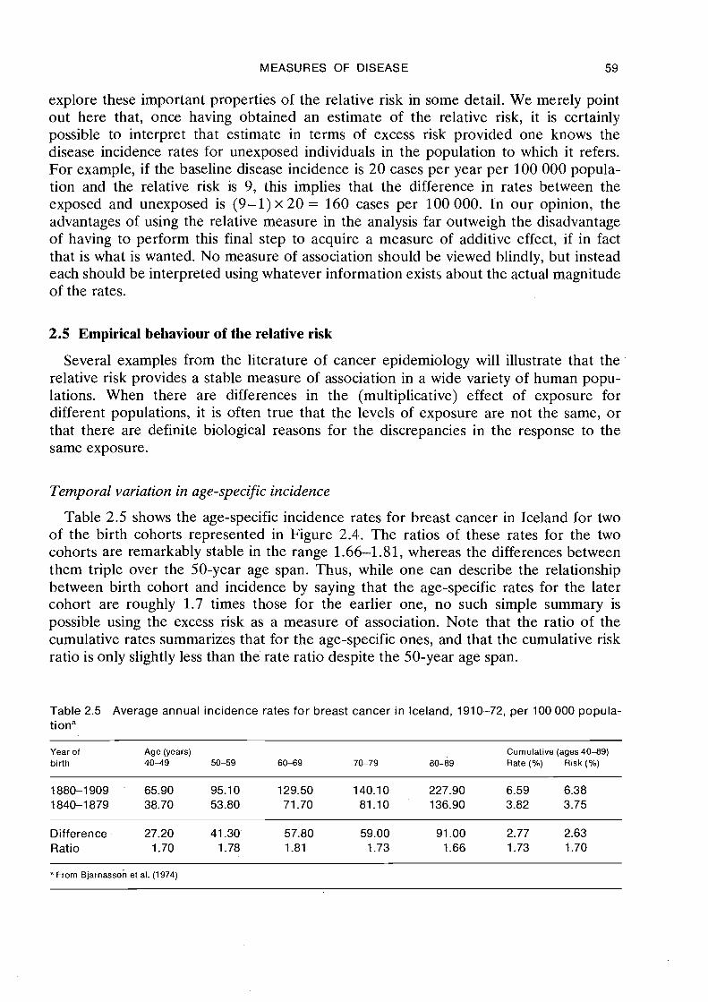
Table 2.5 shows the age-specific incidence rates for breast cancer in Iceland for two of the birth cohorts represented in Figure 2.4.. The ratios of these rates for the two cohorts are remarkably stable in the range 1.66-1.81, whereas the differences between them triple over the 50-year age span. Thus, while one can describe the relationship between birth cohort and incidence by saying that the age-specific rates for the later cohort are roughly 1.7 times those for the earlier one, no such simple summary is possible using the excess risk as a measure of association. Note that the ratio of the cumulative rates summarizes that for the age-specific ones, and that the cumulative risk ratio is only slightly less than .the rate ratio despite the 50-year age span.
Table 2.5 Average annual incidence rates for breast cancer in Iceland, 1910-72, per 100 000 popula- tiona
Year of Age (years) Cumulative (ages 40-89) birth 4 0 4 9 50-59 60-69 70-79 80-89 Rate (%) Risk (%)
Difference 27.20 41.30' 57.80 59.00 91 .OO 2.77 2.63 Ratio 1.70 1.78 1.81 1.73 1.66 1.73 1.70
From ~jarnasson et al. (1974)
60 BRESLOW & DAY
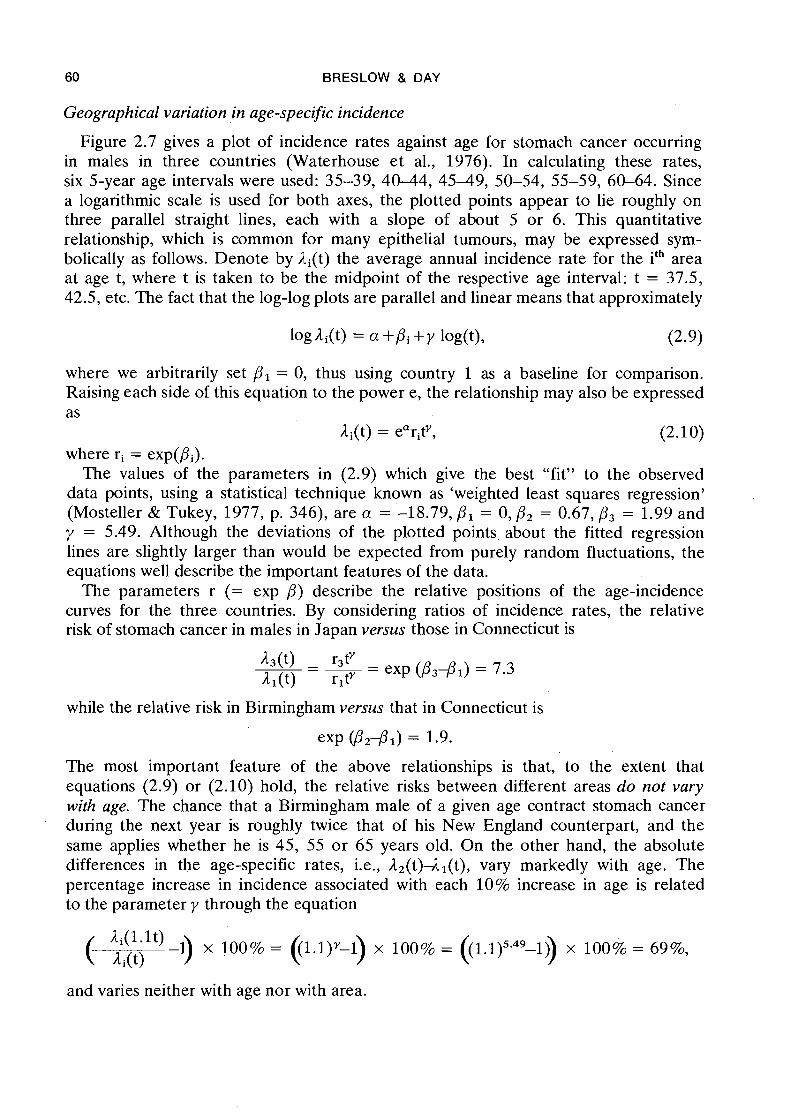
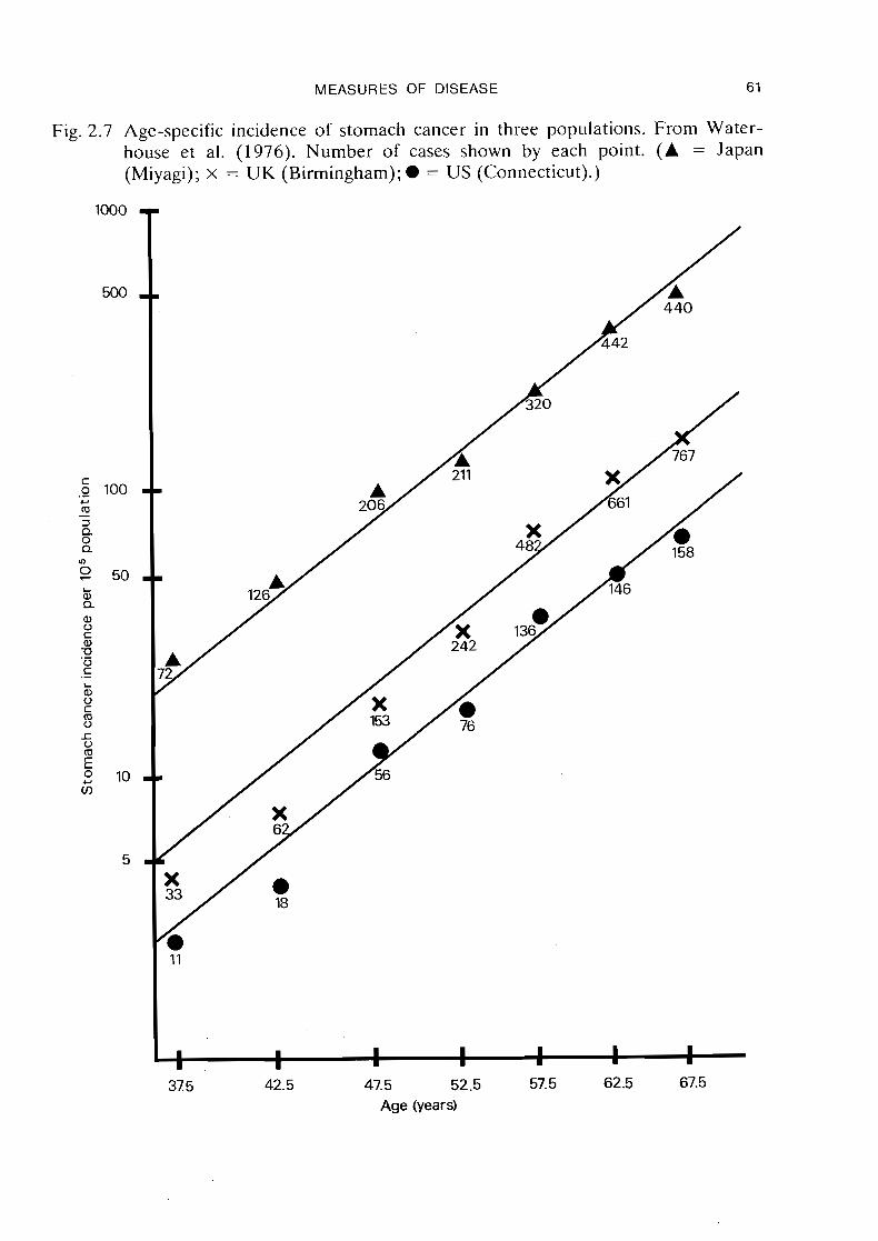
Geographical variation in age-specific incidence
Figure 2.7 gives a plot of incidence rates against age for stomach cancer occurring in males in three countries (Waterhouse e t al., 1976). In calculating these rates, six 5-year age intervals were used: 35-39, 40-4.4, 4 5 4 9 , 50-54, 55-59, 60-64. Since a logarithmic scale is used for both axes, the plotted points appear to lie roughly on three parallel straight lines, each with a slope of about 5 or 6. This quantitative relationship, which is common for many epithelial tumours, may be expressed sym- bolically as follows. Denote by &(t) the average annual incidence rate for the ith area at age t, where t is taken to be the midpoint of the respective age interval: t = 37.5, 42.5, etc. The fact that the log-log plots are parallel and linear means that approximately
where we arbitrarily set PI = 0, thus using country 1 as a baseline for comparison. Raising each side of this equation to the power e, the relationship may also be expressed as
Ai(t) = earitY, (2.10) where ri = exp(Pi).
The values of the parameters in (2.9) which give the best "fit" to the observed data points, using a statistical technique known as 'weighted least squares regression' (Mosteller & Tukey, 1977, p. 346), are a = -18.79, PI = 0, P2 = 0.67, P3 = 1.99 and y = 5.49. Although the deviations of the plotted points about the fitted regression lines are slightly larger than would be expected from purely random fluctuations, the equations well describe the important features of the data.
The parameters r (= exp P) describe the relative positions of the age-incidence curves for the three countries. By considering ratios of incidence rates, the relative risk of stomach cancer in males in Japan versus those in Connecticut is
while the relative risk in Birmingham versus that in Connecticut is
exp @I2d1) = 1.9.
The most important feature of the above relationships is that, to the extent that equations (2.9) or (2.10) hold, the relative risks between different areas d o not vary with age. The chance that a Birmingham male of a given age contract stomach cancer during the next year is roughly twice that of his New England counterpart, and the same applies whether he is 45, 55 o r 65 years old. On the other hand, the absolute differences in the age-specific rates, i.e., J-,(t)A1(t), vary markedly with age. The percentage increase in incidence associated with each 10% increase in age is related to the parameter y through the equation
and varies neither with age nor with area.
a
31 5 42.5 47.5 52.5 57.5 62.5 67.5 Age (years)
62 BRESLOW & DAY
As shown by Cook, Doll & Fellingham (1969), most epithelial tumours have age- incidence curves of a similar shape to .that of gastric cancer, differing between popula- tions only by a proportionality constant, i.e., relative risk. This is a good technical reason for choosing the ratio as a measure of association, since it permits the relation- ship between each pair of age-incidence curves to be quite accurately summarized in a single number.
The two epithelial tumours which deviate most markedly from this pattern are those of the lung and the breast. For breast cancer we have already shown how irregularities in the cross-sectional age curves reflect a changing incidence by year of birth, and that a basic regular behaviour is seen when the data are considered on a cohort basis (Figures 2.3 and 2.4; Bjarnasson et al., 1974). A similar phenomenon has been noted for lung cancer, where a large part of the inter-cohort differences are presumably due to increasing exposure to tobacco and other exogenous agents (Doll, 197 1).
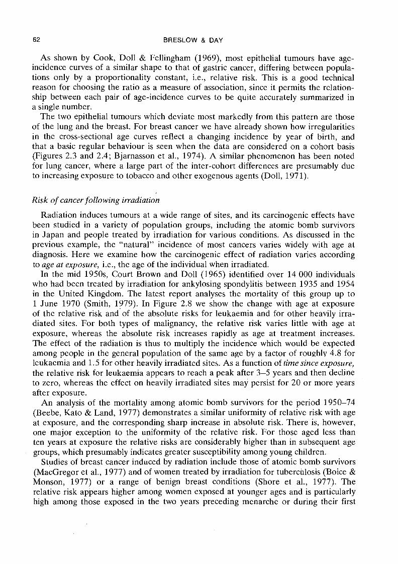
Risk of cancer following irradiation
Radiation induces tumours at a wide range of sites, and its carcinogenic effects have been studied in a variety of population groups, including the atomic bomb survivors in Japan and people treated by irradiation for various conditions. As discussed in the previous example, the "natural" incidence of most cancers varies widely with age at diagnosis. Here we examine how the carcinogenic effect of radiation varies according to age at exposure, i.e., the age of the individual when irradiated.
In the mid 1950s, Court Brown and Doll (1965) identified over 14'000 individuals who had been treated by irradiation for ankylosing spondylitis between 1935 and 1954 in the United Kingdom. The latest report analyses the mortality of this group up to 1 June 1970 (Smith, 1979). In Figure 2.8 we show the change with age at exposure of the relative risk and-of the absolute risks for leukaemia and for other heavily irra- diated sites. For both types of malignancy, the relative risk varies little with age at exposure, whereas the absolute risk increases rapidly as age at treatment increases. The effect of the radiation is thus to multiply the incidence which would be expected among people in the general population of the same age by a factor of rounhlv 4.8 for leukaemia and 1.5 for other heavily irradiated sites. As a function of time since exposure, the relative risk for leukaemia appears to reach a peak after 3-5 years and then decline to zero, whereas the effect on heavily irradiated sites may persist for 20 or more years after exposure.
An analysis of the mortality among atomic bomb survivors for the period 1950-74 (Beebe, Kato & Land, 1977) demonstrates a similar uniformity of relative risk with age at exposure, and the corresponding sharp increase in absolute risk. There is, however, one major exception to the uniformity of the relative risk. For those aged less than ten years at exposure the relative risks are considerably higher than in subsequent age groups, which presumably indicates greater susceptibility among young children.
Studies of breast cancer induced by radiation include those of atomic bomb survivors (MacGregor et al., 1977) and of women treated by irradiation for tuberchlosis (Boice & Monson, 1977) or a range of benign breast conditions (Shore et al., 1977). The relative risk appears higher among women exposed at younger ages and is particularly high among those exposed in the two years preceding menarche or during their first
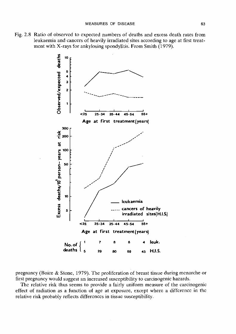
MEASURES OF DISEASE 63
Fig. 2.8 Ratio of observed to expected numbers of deaths and excess death rates from leukaemia and cancers of heavily irradiated sites according to age at first treat- ment with X-rays for ankylosing spondylitis. From Smith (1979).
Age at first treatment (years)
- / ,---- cancers of heavily irradiated si tes(H.1.S.)
Age at first treatment (years)
No.of { 7 8 8 4 leuk.
deaths 29 80 6s 43 H.I.S.
pregnancy (Boice & Stone, 1979). The proliferation of breast tissue during menarche or first pregnancy would suggest an increased susceptibility to carcinogenic hazards.
The relative risk thus seems to provide a fairly uniform measure of the carcinogenic effect of radiation as a function of age at exposure, except where a difference in the relative risk probably reflects differences in tissue susceptibility.
64 BRESLOW & DAY
Lung cancer and cigarette smoking
Smoking and irradiation are perhaps the most extensively studied of all carcinogenic exposures. Cigarette smoking is related to tumours at a number of sites including the respiratory tract, the oral cavity and oesophagus, and the bladder and pancreas. The relationship with cancer of the lung has been the most extensively studied, and the results of several large prospective studies have quantified the association in some detail.
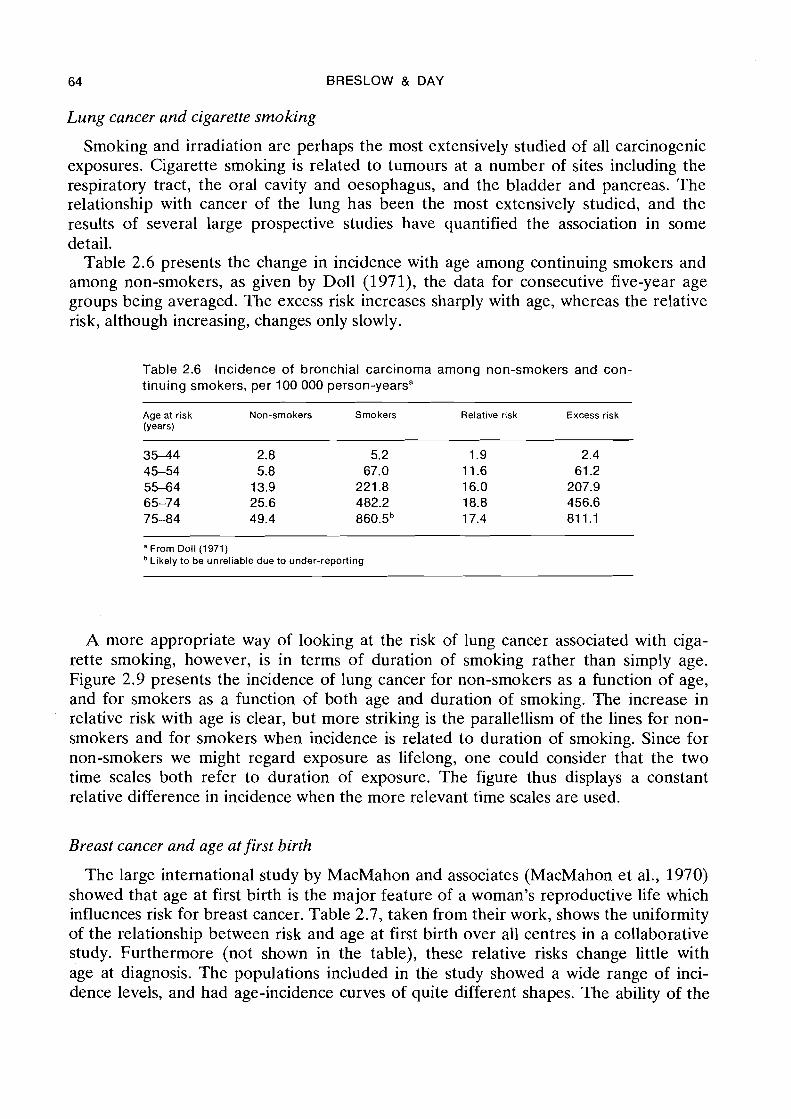
Table 2.6 presents the change in incidence with age among continuing smokers and among non-smokers, as given by Doll (1971), the data for consecutive five-year age groups being averaged. The excess risk increases sharply with age, whereas the relative risk, although increasing, changes only slowly.
Table 2.6 Incidence of bronchial carcinoma among non-smokers and con- tinuing smokers, per 100 000 person-yearsa
Age at risk Non-smokers Smokers Relative risk Excess risk (Years)
"From Doll (1971) Likely to be unreliable due to under-reporting
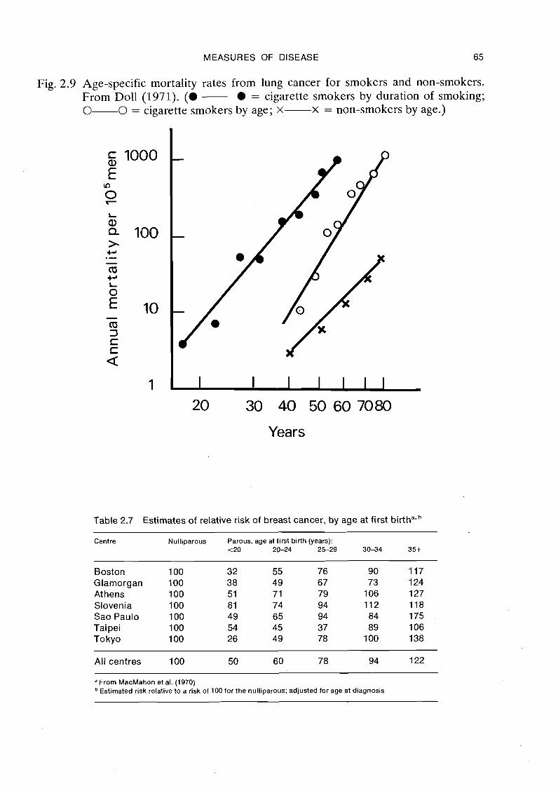
A more appropriate way of looking at the risk of lung cancer associated with ciga- rette smoking, however, is in terms of duration of smoking rather than simply age. Figure 2.9 presents the incidence of lung cancer for non-smokers as a function of age, and for smokers as a function of both age and duration of smoking. The increase in relative risk with age is clear, but more striking is the parallellism of the lines for non- smokers and for smokers when incidence is related to duration of smoking. Since for non-smokers we might regard exposure as lifelong, one could consider that the two time scales both refer to duration of exposure. The figure thus displays a constant relative difference in incidence when the more relevant time scales are used.
Breast cancer and age at first birth
The large international study by MacMahon and associates (MacMahon et al., 1970) showed that age at first birth is the major feature of a woman's reproductive life which influences risk for breast cancer. Table 2.7, taken from their work, shows the uniformity of the relationship between risk and age at first birth over all centres in a collaborative study. Furthermore (not shown in the table), these relative risks change little with age at diagnosis. The populations included in the study showed a wide range of inci- dence levels, and had age-incidence curves of quite different shapes. The ability of the
MEASURES OF DISEASE 65
Fig. 2.9 Age-specific mortality rates from lung cancer for smokers and non-smokers. From Doll (1971). ( a - l = cigarette smokers by duration of smoking; 0-0 = cigarette smokers by age; x-x = non-smokers by age.)
20 30 40 50 60 7080
Years
Table 2.7 Estimates of relative risk of breast cancer, by age at first birthavb
Centre Nulliparous Parous, age at first birth (years): t 2 0 20-24 2 S 2 9 30-34 35 t
Boston 100 32 55 76 90 117 Glamorgan 100 3 8 49 67 73 1 24 At hens 100 51 71 79 1 06 127 Slovenia 100 81 74 94 112 118 Sao Paulo 100 49 65 94 84 175 Taipei 100 54 45 37 89 106 Tokyo 100 26 49 78 100 138
All centres 100 50 60 78 94 122 -
a From MacMahon et al. (1970) Estimated risk relative to a risk of 100 for the nulliparous; adjusted for age at diagnosis
66 BRESLOW & DAY
relative risk to summarize the relationships among so wide an array of incidence pat- terns indicates that, at least in this situation, it reflects a fundamental feature of the disease. The absolute differences in age-specific incidence rates by age at first birth vary widely between the populations.
The failure of previous work on the influence of reproductive factors on risk of breast cancer to identify the basic importance of age at first birth was probably due to inappropriate measures of disease association. As MacMahon et al. concluded, "Previous workers seem not to have considered the differences of sufficient importance to warrant detailed exploration. An apparent lack of interest in the relationship may have resulted from failure to realize the magnitude of the differences in relative risk that underlie it. This lack of recognition of the strength of the relationship can be attributed primarily to analyses using summary statistics such as means . . .".
2.6 Effects of combined exposures
The previous examples have illustrated the extent to which the relative risk remains constant over different age strata, or among different population groups. We shall now examine the extent to which the relative risk associated with one risk factor varies with changing exposure to a second risk factor, and we shall see that in this situation one also frequently observes relative uniformity. Consider the simplest situation, with two dichotomous variables A and B. There are four incidence rates, denoted LAB, LA, lB and lo according to whether an individual is exposed to both, one or neither of the factors. The three relative risks, expressed using lo as the baseline incidence, are rAB = lAB/AO, rA = lA/10 and rB = AB/AO, respectively.
Among those exposed to B, the relative increase in risk incurred by also being exposed to A is given by lAB/ lB = rAB/rB. If the relative risk associated with exposure to A is the same, whether or not there is exposure to B, we say that the effects of the two factors are independent or do not interact (Figure 2.6). In this case rAB/rB = rA, from which TAB = rArB. Thus, the independence of relative risks for two or more exposures implies a multiplicative combination for the joint effect. But, if the two risk factors each have additive rather than multiplicative effects on incidence, then similar calculations show that the relative risk for the joint exposure under the no interaction assumption is rAB = rA + rB-1.
The uniformity of relative risk for the exposures considered in the earlier examples can also be interpreted as a multiplicative combination of effects. Since the spontaneous incidence of leukaemia increases with age and radiation affects the spontaneous inci- dence proportionately, the joint effect is simply the product of the spontaneous rate and the radiation risk. Women in the United States have an incidence of breast cancer about six times higher than that of Japanese women. The joint action of the factor responsible for the elevated risk among United States women, whatever it may be, and age at first birth is clearly multiplicative.
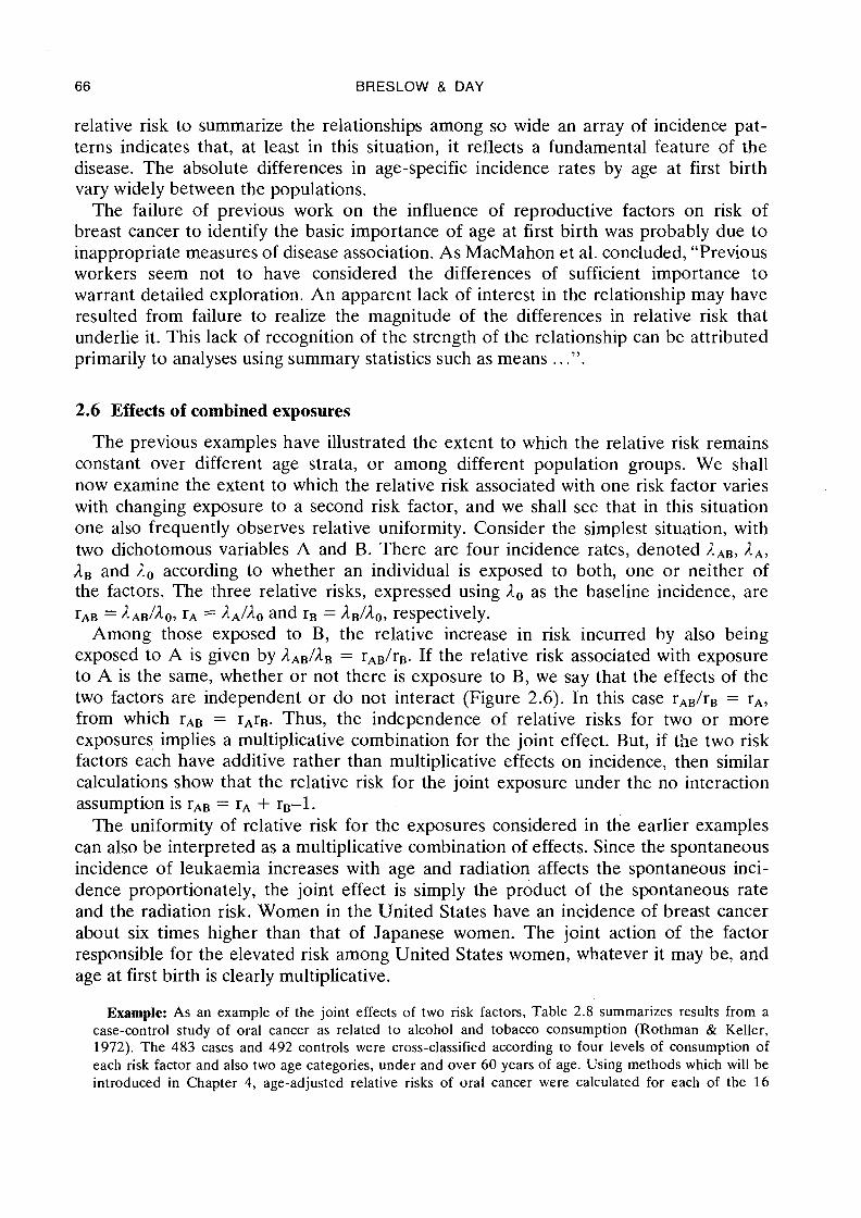
Example: As an example of the joint effects of two risk factors, Table 2.8 summarizes results from a case-control study of oral cancer as related to alcohol and tobacco consumption (Rothman & Keller, 1972). The 483 cases and 492 controls were cross-classified according to four levels of consumption of each risk factor and also two age categories, under and over 60 years of age. Using methods which will be introduced in Chapter 4, age-adjusted relative risks of oral cancer were calculated for each of the 16
MEASURES OF DISEASE 67
Table 2.8 Joint effect of alcohol and tobacco consumption on risk for oral
Alcohol Tobacco (cigarette equiv.1day) Alcohol risk (ozlday) 0 1-19 20-39 40+ (adjusted for tobacco)
0 1 .O 1.6 1.6 3.4 1 .O 0.14.3 1.7 1.9 3.3 3.4 1.8 0.4-1.5 1.9 4.9 4.9 8.2 2.9 1.6+ 2.3 4.8 10.0 15.6 4.2
Tobacco risk 1 .O 1.4 2.4 4.2 (adjusted for alcohol)
"From Rothman and Keller (1972) Relative risks adjusted for age at diagnosis
alcohol/tobacco categories shown. These may be denoted rij, where i refers to tobacco level and j to alcohol level. Since the category of lowest exposure to both factors is used as a baseline for comparison with other groups, r,, = 1.0.
The multiplicative hypothesis in this framework takes the form
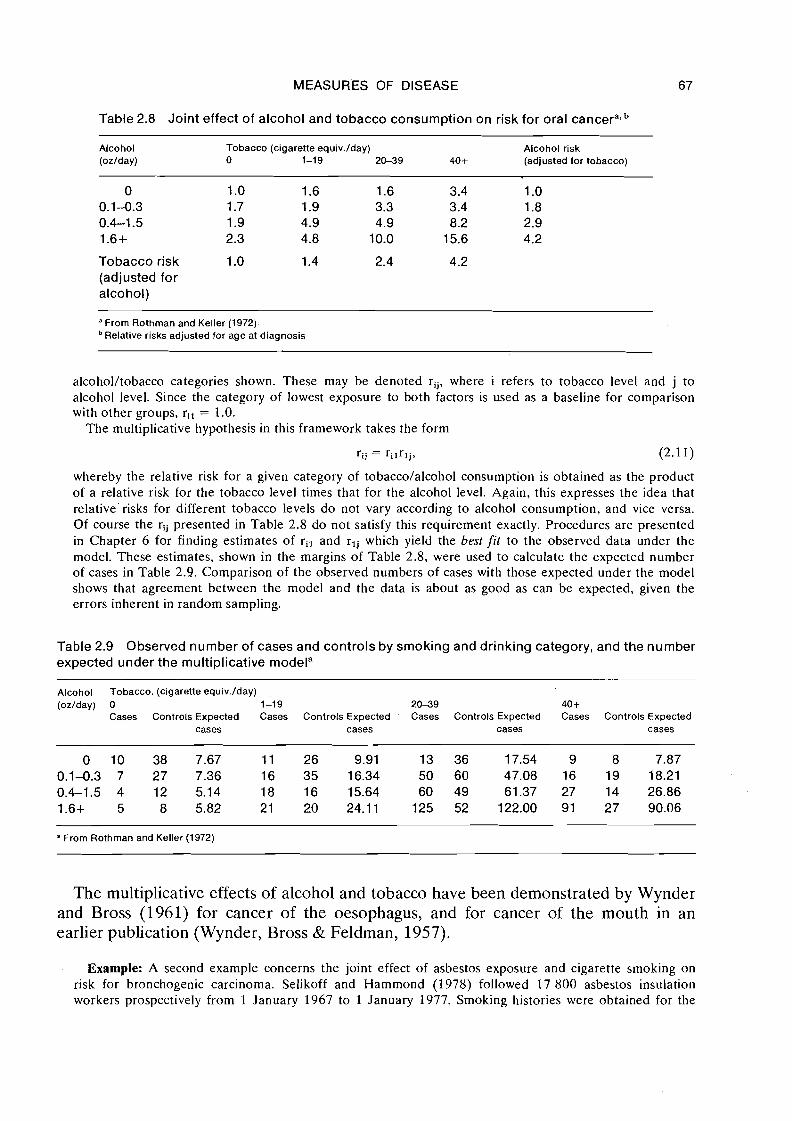
whereby the relative risk for a given category of tobacco/alcohol consumption is obtained as the product of a relative risk for the tobacco level times that for the alcohol level. Again, this expresses the idea that relative risks for different tobacco levels do not vary according to alcohol consumption, and vice versa. Of course the rij presented in Table 2.8 do not satisfy this requirement exactly. Procedures are presented in Chapter 6 for finding estimates of ril and rlj which yield the best fit to the observed data under the model. These estimates, shown in the margins of Table 2.8, were used to calculate the expected number of cases in Table 2.9. Comparison of the observed numbers of cases with those expected under the model shows that agreement between the model and the data is about as good as can be expected, given the errors inherent in random sampling.
Table 2.9 Observed number of cases and controls by smoking and drinking category, and the number expected under the multiplicative modela
Alcohol Tobacco. (cigarette equiv.1day) (ozlday) 0 1-19 2 0 3 9 40 +
Cases Controls Expected Cases Controls Expected ' Cases Controls Expected Cases Controls Expected cases cases cases cases
a From Rothman and Keller (1972)
The multiplicative effects of alcohol and tobacco have been demonstrated by Wynder and Bross (1961) for cancer of the oesophagus, and for cancer of the mouth in an earlier publication (Wynder, Bross & Feldman, 1957).
Example: A second example concerns the joint effect of asbestos exposure and cigarette smoking on risk for bronchogenic carcinoma. Selikoff and Hammond (1978) followed 17 800 asbestos insulation workers prospectively from 1 January 1967 to 1 January 1977. Smoking histories were obtained for the
68 BRESLOW & DAY
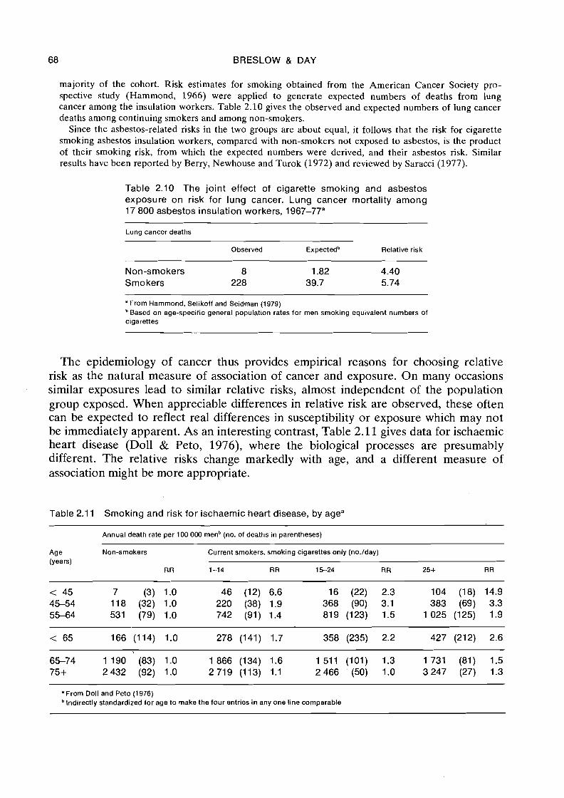
majority of the cohort. Risk estimates for smoking obtained from the American Cancer Society pro- spective study (Hammond, 1966) were applied to generate expected numbers of deaths from lung cancer among the insulation workers. Table 2.10 gives the observed and expected numbers of lung cancer deaths among continuing smokers and among non-smokers.
Since the asbestos-related risks in the two groups are about equal, it follows that the risk for cigarette smoking asbestos insulation workers, compared with non-smokers not exposed to asbestos, is the product of their smoking risk, from which the expected numbers were derived, and their asbestos risk. Similar results have been reported by Berry, Newhouse and Turok (1972) and reviewed by Saracci (1977).
Table 2.10 The joint effect of cigarette smoking and asbestos exposure on risk for lung cancer. Lung cancer mortality among 17 800 asbestos insulation workers, 1967-77"
Lung cancer deaths
Observed Expectedb Relative risk
Non-smokers 8 1.82 4.40 Smo kers 228 39.7 5.74
"From Hammond, Selikoff and Seidman (1979) Based on age-specific general population rates for men smoking equivalent numbers of
cigarettes
The epidemiology of cancer thus provides empirical reasons for choosing relative risk as the natural measure of association of cancer and exposure. On many occasions similar exposures lead to similar relative risks, almost independent of the population group exposed. When appreciable differences in relative risk are observed, these often can be expected to reflect real differences in susceptibility or exposure which may not be immediately apparent. As an interesting contrast, Table 2.11 gives data for ischaemic heart disease (Doll & Peto, 1976), where the biological processes are presumably different. The relative risks change markedly with age, and a different measure of association might be more appropriate.
Table 2.1 1 Smoking and risk for ischaemic heart disease, by agea
Annual death rate per 100 000 menb (no. of deaths in parentheses)
Age Non-smokers Current smokers, smoking cigarettes only (no./day) (years)
R R 1-14 R R 15-24 R R 25+ RR
" From Doll and Peto (1 976) Indirectly standardized for age to make the four entries in any one line comparable
MEASURES OF DISEASE 69
2.7 Logical properties of the relative risk
In addition to an empirical justification for its use, the relative risk has some pro- perties of a logical nature which are useful for appraising the extent to which the observed association may be explained by the presence of another agent, or may be specific to a particular disease entity. Cornfield et al. (1959) gave a precise statement and formal proof of these properties (see also 5 2.9).
"If an agent, A, with no causal effect upon the risk of disease, nevertheless, because of a positive correlation with some other causal agent, B, shows an apparent risk, r, for those exposed to A, relative to those not so exposed, then the prevalence of B, among those exposed to A, relative to the prevalence among those not so exposed, must be greater than r."
Thus, in order that the smoking-lung cancer association be explained by a tendency for people with a cancer-causing genotype to smoke, the putative genetic trait must carry a risk of at least ninefold in addition to being at least nine times more prevalent among smokers. Spurious associations due to confounding are always weaker than the underlying genuine associations when strength of association is measured by relative risk.
Cornfield et al. also note that the relative measure is a sensitive indicator of the speci- ficity of the association with a particular disease entity:
"If a causal agent A increases the risk for disease I and has no effect on the risk for disease 11, then the relative risk of developing disease I, alone, is greater than the relative risk of developing disease I and I1 combined, while the absolute measure is unaffected."
Thus, if the agent in question increases the risk of a certain histological type of cancer at a given site (e.g., "epidermoid" as opposed to other types of lung cancer) but has little or no effect on other types, a greater relative risk is obtained when the calculation is restricted to the particular histological type than when all cancers at that site are considered. But, it makes no difference to the excess risk if the other histological types are included or not.
Finally, from the point of view of case-control studies, there is one compelling reason for adopting the relative risk as the primary measure of association even in the absence of other considerations. This is simply that, as shown in the next section, the relative risk is in principle directly estimable from data collected in a case-control study. Addi- tional information, namely knowledge of actual incidence rates for at least one of the exposed or non-exposed populations, is required to estimate the excess risk.
2.8 Estimation of the relative risk from case-control studies - basic concepts
A full understanding of how .the data from a case-control study permit estimation of the relative risk requires careful description of how cases and controls are sampled from the population. The studies whose analysis is considered in this monograph involve the ascertainment of new (incident) cases which occur in a defined study period. Ideally these cases are identified through a cancer registry or some other system which
70 BRESLOW & DAY
covers a well-defined population; with hospital-based studies the referent population, consisting of all those "served" by the given hospital, may be more imaginary than real. Most commonly the sample will contain all new cases arising during the study period, or at least all those successfully interviewed. Otherwise they are assumed to be a random sample of the actual cases.
The controls in a case-control study are assumed to represent a random sample of the subjects who are disease-free, though otherwise at risk. The control sample may be stratified, for example on the basis of age and sex, so that it has roughly the same age and sex distribution as the cases. Or, the controls may be individually matched to cases on the basis of family membership, residence or other characteristics. Under such circumstances the controls are assumed to constitute a random sample from within each of the subpopulations formed by the stratification or matching factors.
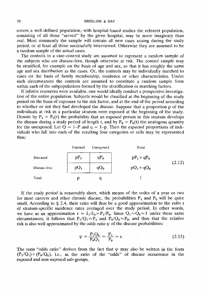
If infinite resources were available, one would ideally conduct a prospective investiga- tion of the entire population. Subjects would be classified at the beginning of the study period on the basis of exposure to the risk factor, and at the end of the period according to whether or not they had developed the disease. Suppose that a proportion p of the individuals at risk in a particular stratum were exposed at the beginning of the study. Denote by Pi = Pl(t) the probability that an exposed person in this stratum develops the disease during a study period of length t, and by Po = Po(t) the analogous quantity for the unexposed. Let Q = 1-P and q = 1-p. Then the expected proportions of indi- viduals who fall into each of the resulting four categories or cells.may be represented thus:
Exposed Unexposed Total
Diseased
Total P ‘I 1
If the study period is reasonably short, which means of the order of a year or two for most cancers and other chronic disease, the probabilities Pi and Po will be quite small. According to 5 2.4, their ratio will thus be a good approximation to the ratio r of stratum-specific incidence rates averaged over the study period. In other words, we have as an approximation r = ll/lo-Pl/Po. Since Q1 =Qo= 1 under these same circumstances, it follows that Pl/Ql ==PI and Po/Qo=Po, and thus that the relative risk is also well approximated by the odds ratio w of the disease probabilities:
The term "odds ratio" derives from the fact that $J may also be written in the form (Pl/Ql)+(Po/Qo), i.e., as the ratio of the "odds" of disease occurrence in the exposed and non-exposed sub-groups.
MEASURES OF DISEASE 71
Example: Suppose the average annual incidence rates for the exposed and non-exposed substrata are A , = 0.02 and A, = 0.01 and that the study lasts three years. Then the cumulative rates are A , = 0.06 and A. = 0.03, while the corresponding risks (2.4) are PI = 1 - exp(-0.06) = 0.05824 and Po = 1 - exp(-0.03) = 0.02956. It follows that the odds ratio is
as compared with a relative risk r = l1/AO of exactly 2.
As Cornfield (195 1) observed, the approximation (2.13) provides the critical link between prospective and retrospective (case-control) studies vis-a-vis estimation of the relative risk. If the entire population were kept under observation for the duration of the study, separate estimates would be available for each of the quantities p, PI and Po, so that one could determine all the probabilities shown in (2.12). If we were to take samples of exposed and unexposed individuals at the beginning. of the study and follow them up, this would permit estimation of PI and Po and thus of both excess and relative risks, but not of p; of course such samples would have to be rather large in order to permit sufficient cases to be observed to obtain good estimates. With the case-control approach, on the other hand, sampling is done according to disease rather than exposure status. This ensures that a reasonably large number of diseased persons will be included in the study. From such samples of cases and controls one may estimate the exposure probabilities given disease status, namely:
p1 = pr(exposed 1 case) = PPI and pP1+ qpo
po = pr(exposed 1 control) = PQI pQl+ qQo
It immediately follows that the odds ratio calculated from the exposure probabilities is identical to the odds ratio of the disease probabilities, or in symbols:
Consequently the ratio of disease incidences, as approximated by the odds ratio of the corresponding risks, can be directly estimated from a case-control study even though the latter provides no information ahout the absolute magnitude of the incidence rates in the exposed and non-exposed subgroups.
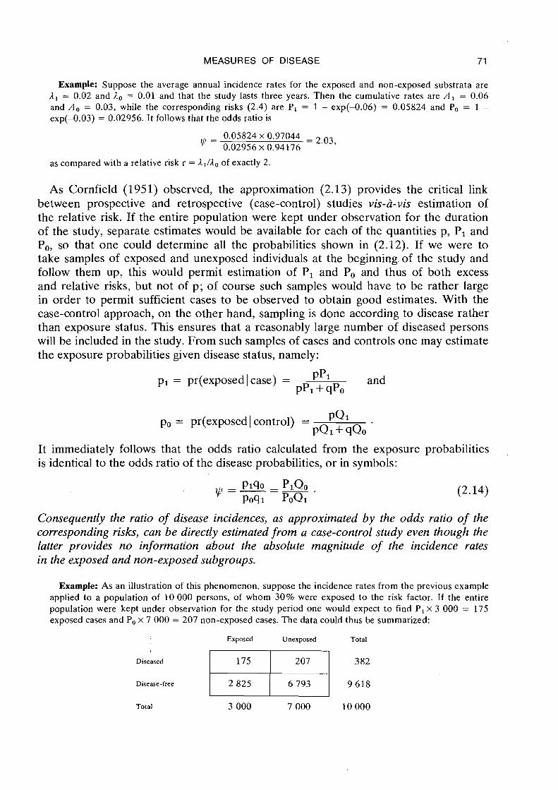
Example: As an illustration of this phenomenon, suppose the incidence rates from the previous example applied to a population of 10 000 persons, of whom 30% were exposed to the risk factor. If the entire population were kept under observation for the study period one would expect to find P, x 3 000 = 175 exposed cases and Po x 7 000 = 207 non-exposed cases. The data could thus be summarized:
Exposed Unexposed Total
Total 3 000 7 000 10 000
72 BRESLOW & DAY
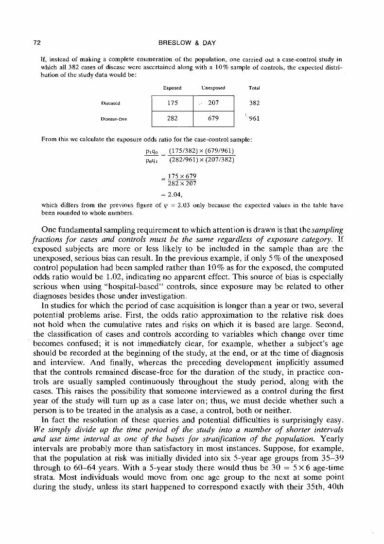
If, instead of making a complete enumeration of the population, one carried out a case-control study in which all 382 cases of disease were ascertained along with a 10% sample of controls, the expected distri- bution of the study data would be:
Exposed Unexposed Total
Diseased
Disease-free
From this we calculate the exposure odds ratio for the case-control sample:
which differs from the previous figure of yp = 2.03 only because the expected values in the table have been rounded to whole numbers.
One fundamental sampling requirement to which attention is drawn is that thesampling fractions for cases and controls must be the same regardless of exposure category. If exposed subjects are more or less likely to be included in the sample than are the unexposed, serious bias can result. In the previous example, if only 5 % of the unexposed control population had been sampled rather than 10% as for the exposed, the computed odds ratio would be 1.02, indicating no apparent effect. This source of bias is especially serious when using "hospital-based" controls, since exposure may be related to other diagnoses besides those under investigation.
In studies for which the period of case acquisition is longer than a year or two, several potential problems arise. First, the odds ratio approximation to the relative risk does not hold when the cumulative rates and risks on which it is based are large. Second, the classification of cases and controls according to variables which change over time becomes confused; it is not immediately clear, for example, whether a subject's age should be recorded at the beginning of the study, at the end, or at the time of diagnosis and interview. And finally, whereas the preceding development implicitly assumed that the controls remained disease-free for the duration of the study, in practice con- trols are usually sampled continuously throughout the study period, along with the cases. This raises the possibility that someone interviewed as a control during the first year of the study will turn up as a case later on; thus, we must decide whether such a person is to be treated in the analysis as a case, a control, both or neither.
In fact the resolution of these queries and potential difficulties is surprisingly easy. W e simply divide up the time period of the study into a number of shorter intervals and use time interval as one of the bases for stratification of the population. Yearly intervals are probably more than satisfactory in most instances. Suppose, for example, that the population at risk was initially divided into six 5-year age groups from 35-39 through to 60-64 years. With a 5-year study there would thus be 30 = 5 x 6 age-time strata. Most individuals would move from one age group to the next at some point during the study, unless its start happened to correspond exactly with their 35th, 40th
MEASURES OF DISEASE 73
or similar birthday. A separate estimate of the relative risk would be obtained for each stratum by computing the odds ratio of the exposure probability of cases and controls in the usual fashion. If the 30 estimates appeared reasonably stable with respect to age and time, they would be combined into a single summary of relative risk for the entire population. Otherwise variations in the relative risk could be modelled as a function of age and/or time in the statistical analysis.
Partition of the study period into several time intervals resolves each of the problems mentioned above. First, by making the intervals sufficiently short, the cumulative incidence rates over each one are guaranteed to be so small as to be virtually indistin- guishable from the cumulative risks; this means that the odds ratio approximation to each relative risk will involve negligible error. Second, the fact that ages are changing throughout the study period is explicitly accounted for in that each case and control is assigned to the appropriate age category in which he finds himself at the time of ascertainment; in practice this means that ages are recorded at the time of interview, as is commonly done anyway. Finally, while such an event would usually be rare, a person could be included as both a case and a control; having been sampled as a disease-free control at one time, he might develop the disease later on and thus be re-interviewed as a case. Exclusion of either of his interview records from the statistical analysis would, technically speaking, bias the result.
It is of interest to consider the limiting form of such a partition of the study period in which the time intervals become arbitrarily small. The effect is that each case is matched with one or more controls who are disease-free at the precise moment that the case is diagnosed. Such controls are usually chosen to be of the same age and sex and may have other features in common as well. This approach, which in fact accords reasonably well with the actual conduct of many studies, avoids completely the odds ratio approximation to the relative risk since the relevant time periods are infinitesimally small. It implies, however, that the resultant data are analysed so as to preserve intact the matched sets of case and control(s). Prentice and Breslow (1978) present a more mathematical account of this idea, while in Chapters 5 and 7 we discuss methods of analysis appropriate for matched data collected in this fashion [see also Liddell et al. (1 977)l.
In the sequel we will use repeatedly and without further comment the odds ratio approximation to the relative risk, assuming that the conditions for its validity as out- lined here have been met for the data being analysed.
2.9 Attributable risk and related measures
Case-control studies provide direct estimates of the relative increase in incidence associated with an exposure. They may also yield unbiased estimates of the distribution of exposure levels in the population, provided of course that the control samples have been drawn from the population at risk according to a well-defined sampling scheme, rather than on the basis of matching to individual cases. By combining the information about the distribution of exposures with the estimates of relative risk, one can determine the degree to which cases of disease occurring in the population are explained by the exposure. Likewise, knowledge of the differences in the distribution of exposure among two or more populations permits calculation of the extent to which differences in risk
74 BRESLOW & DAY
between them are due to confounding by the exposure. In this section we explore briefly a few such auxiliary measures derived from the relative risk. While these are useful in interpreting the results of a study, questions on the statistical significance of .the results should be directed primarily towards the relative risk.
In order to simplify the discussion, let us ignore the possible agelsexltime variation in incidence rates. Suppose that ,Io and ,I1 denote the overall incidence rates for the non-exposed and exposed subgroups and let r=,Il/,Io represent the relative risk. Then the proportion of the cases of disease occurring among exposed persons which is in excess in comparison with the non-exposed is
a quantity which has been labelled by Cole & MacMahon (1971) as the attributable risk for. e x p ~ s e d ' ~ e r s o n s . If p denotes the proportion of persons in the population exposed to the risk factor, then the total disease incidence is
The excess among the exposed is given by p(,Il-,Io), from which one arrives at the expression
for the population attributable risk (AR), first described by Levin (1953). This repre- sents the proportion of cases occurring in the total population which can be explained by the risk factor. Walter (1975) has investigated some of the statistical properties of this measure.
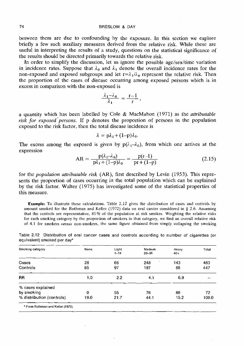
Example: To illustrate these calculations. Table 2.12 gives the distribution of cases and controls by amount smoked for the Rothman and Keller (1972) data on oral cancer considered in 5 2.6. Assuming that the controls are representative, 81 % of the population at risk smokes. Weighting the relative risks for each smoking category by the proportion of smokers in that category, we find an overall relative risk of 4.1 for smokers versus non-smokers, the same figure obtained from simply collapsing the smoking
Table 2.12 Distribution of oral cancer cases and controls according to number of cigarettes (or equivalent) smoked per daya
Smoking category None Light Medium Heavy Total 1-19 20-39 40+
Cases Controls
RR 1 .O 2.2 4.1 6.9 -
% cases explained by smoking 0 55 76 88 72 Oh distribution (controls) 19.0 21.7 44.1 15.2 100.0
- - - - --
a From Rothrnan and Keller (1972)
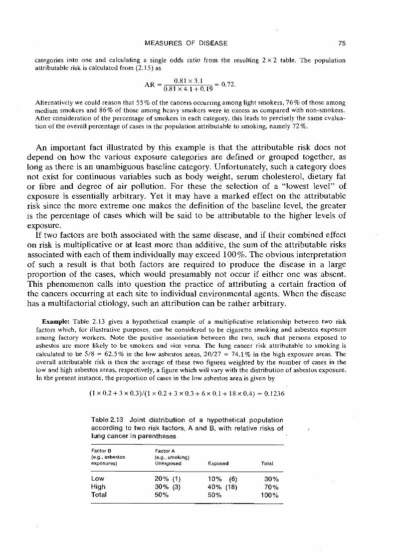
MEASURES OF DISEASE 75
categories into one and calculating a single odds ratio from the resulting 2 x 2 table. The population attributable risk is calculated from (2.15) as
Alternatively we could reason that 55 % of the cancers occurring among light smokers, 76% of those among medium smokers and 86% of those among heavy smokers were in excess as compared with non-smokers. After consideration of the percentage of smokers in each category, this leads to precisely the same evalua- tion of the overall percentage of cases in the population attributable to smoking, namely 72%.
An important fact illustrated by this example is that the attributable risk does not depend on how the various exposure categories are defined or grouped together, as long as there is an unambiguous baseline category. Unfortunately, such a category does not exist for continuous variables such as body weight, serum cholesterol, dietary fat or fibre and degree of air pollution. For these the selection of a "lowest level" of exposure is essentially arbitrary. Yet it may have a marked effect on the attributable risk since the more extreme one makes the definition of the baseline level, the greater is the percentage of cases which will be said to be attributable to the higher levels of exposure.
If two factors are both associated with the same disease, and if their combined effect on risk is multiplicative or at least more than additive, the sum of the attributable risks associated with each of them individually may exceed 100%. The obvious interpretation of such a result is that both factors are required to produce the disease in a large proportion of the cases, which would presumably not occur if either one was absent. This phenomenon calls into question the practice of attributing a certain fraction of the cancers occurring at each site to individual environmental agents. When the disease has a multifactorial etiology, such an attribution can be rather arbitrary.
Example: Table 2.13 gives a hypothetical example of a multiplicative relationship between two risk factors which, for illustrative purposes, can be considered to be cigarette smoking and asbestos exposure among factory workers. Note the positive association between the two, such that persons exposed to asbestos are more likely to be smokers and vice versa. The lung cancer risk attributable to smoking is calculated to be 5/8 = 62.5% in the low asbestos areas, 20/27 = 74.1% in the high exposure areas. The overall attributable risk is then the average of these two figures weighted by the number of cases in the low and high asbestos areas, respectively, a figure which will vary with the distribution of asbestos exposure. In the present instance, the proportion of cases in the low asbestos area is given by
Table 2.13 Joint distribution of a hypothetical population according to two risk factors, A and B, with relative risks of I
lung cancer in parentheses
Factor B Factor A (e.g., asbestos (e.g., smoking) exposures) Unexposed Exposed Total
Low High Total
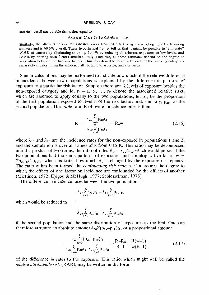
76 BRESLOW & DAY
and the overall attributable risk is thus equal to
Similarly, the attributable risk for asbestos varies from 54.5% among non-smokers to 61.5% among smokers and is 60.6% overall. These hypothetical figures tell us that it might be possible to "eliminate" 70.6% of cancers by eliminating smoking, 59.4% by reducing all asbestos exposures to low levels, and 88.8% by altering both factors simultaneously. However, all these estimates depend on the degree of association between the two risk factors. Thus it is desirable to consider each of the smoking categories separately in determining the incidence attributable to asbestos, and vice versa.
Similar calculations may be performed to indicate how much of the relative difference in incidence between two populations is explained by the difference in patterns of exposure to a particular risk factor. Suppose there are K levels of exposure besides the non-exposed category and let ro = 1, rl, . . ., r~ denote the associated relative risks, which are assumed to apply equally to the two populations; let plk be the proportion of the first population exposed to level k of the risk factor, and, similarly, PZk for the second population. The crude ratio R of overall incidence rates is then
where Ale and are the incidence rates for the non-exposed in populations 1 and 2, and the summation is over all values of k from 0 to K. This ratio may be decomposed into the product of two terms, the ratio of rates Ro = 120/110 which would persist if the two populations had the same patterns of exposure, and a multiplicative factor w = CpZkrk/~plkrk, which indicates how much Ro is changed by the exposure discrepancy. The ratio w has been termed the confounding risk ratio as it measures the degree to which the effects of one factor on incidence are confounded by the effects of another (Miettinen, 1972 ; Eyigou & McHugh, 1977; Schlesselman, 1978).
The difference in incidence rates between the two populations is
which would be reduced to
if the second population had the same distribution of exposures as the first. One can therefore attribute an absolute amount 12&(~2k-~ lk ) rk , or a proportional amount
of the difference in rates to the exposure. This ratio, which might well be called the relative attributable risk (RAR), may be written in the form
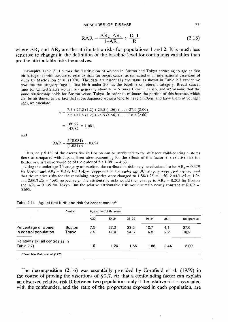
MEASURES OF DISEASE 77
RAR = AR2-AR1 - . R-1
1-AR1 ' R
where AR1 and AR2 are the attributable risks for populations 1 and 2. It is much less sensitive to changes in the definition of the baseline level for continuous variables than are the attributable risks themselves.
Example: Table 2.14 shows the distribution of women in Boston and Tokyo according to age at first birth, together with associated relative risks for breast cancer as estimated in an international case-control study by MacMahon et al. (1970). The data are essentially the same as shown in Table 2.7 except we now use the category "age at first birth under 20" as the baseline or referent category. Breast cancer rates for United States women are generally about R = 5 times those in Japan, and we assume that the same relationship holds for Boston versus Tokyo. In order to estimate the portion of this increase which can be attributed to the fact that more Japanese women tend to have children, and have them at younger ages, we calculate
and
RAR = 5 (0.081)
= 0.094. (1.081) 4
Thus, only 9.4% of the excess risk in Boston can be attributed to the different child-bearing customs there as compared with Japan. Even after accounting for the effects of this factor, the relative risk for Boston versus Tokyo would be of the order of 5 + 1.081 = 4.63.
Using the under age 20 category as baseline, the attributable risks may be calculated to be AR, = 0.379 for Boston and AR, = 0.328 for Tokyo. Suppose that the under age 30 category were used instead, and that the relative risks for the remaining categories were changed to 1.8811.25 = 1.50, 2.4411.25 = 1.95 and 2.0011.25 = 1.60, respectively. The attributable risks would then change to AR, = 0.203 for Boston and AR, = 0.139 for Tokyo. But the relative attributable risk would remain nearly constant at RAR = 0.093.
Table 2.14 Age at first birth and risk for breast cancera
Centre Age at first birth (years)
<20 20-24 25-29 30-34 35 + Nulliparous
Percentage of women Boston 7.5 27.2 23.5 10.7 4.1 27.0 in control population Tokyo 7.5 41.4 24.5 6.2 2.2 18.2
Relative risk (all centres as in Table 2.7) 1 .O 1.20 1.56 1.88 2.44 2.00
"From MacMahon et al. (1970)
The decomposition (2.16) was essentially provided by Cornfield et al. (1959) in the course of proving the assertions of 3 2.7, viz that a confounding factor can explain an observed relative risk R between two populations only if the relative risk r associated with the confounder, and the ratio of the proportions exposed in each population, are
78 BRESLOW & DAY
both even greater than R. Consider the above formulation in the case R = 9, Ro = 1 and K = 1. Let p2 denote the proportion of exposed individuals in population 2 and let pl be the same for population 1. In order for the difference between .these two proportions to explain completely the ninefold excess we must have w>9, i.e., (1-p2) + rp2 > 9{(1-pl) + rpl), which implies both p, > 9p, + 8/(r-1) > 9pl and r > 9.
We end this chapter with a brief word of caution regarding the interpretation of attributable risks, whether relative or absolute. For pedagogic reasons, language was occasionally used which seemed to imply that the elimination of a particular risk factor would result in a measured reduction in incidence. This of course supposes that the as- sociation between risk factor and disease as estimated from the observational study is in fact a causal one. Unfortunately, the only way to be absolutely certain that a causal relationship exists is to intervene actively in the system by removing the disputed factor. In the absence of such evidence, a more cautious interpretation of the attributable risk measures would be in terms of the proportion of risk explained by the given factor, where "explain" is used in the limited sense of statistical association. The next chapter considers in some detail the problem of drawing causal inferences from observational data such as .those collected in case-control studies.
REFERENCES
Beebe, G.W., K to, H. & Land, C.E. (1977) Mortality experience of atomic bomb
Foundation 4 survivors 1950 ;, 74. Life Span Study Report 8, Hiroshima, Radiation Effects Research
Berkson, J. (195 1 ) Smoking and lung cancer: some observations on two recent reports. J. Am. stat. Assoc., 53, 28-38
Berry, G., Newhouse, M.L. & Turok, M. (1972) Combined effect of asbestos exposure and smoking on mortality from lung cancer in factory workers. Lancet, ii, 476-479
Bjarnasson, O., Day, N. E., Snaedal, G. & Tulinius, H. (1974) The effect of year of birth on the breast cancer incidence curve in Iceland. Int. J. Cancer, 13, 689-696
Bogovski, P. & Day, N.E. (1977) Accelerating action of tea on mouse skin carcino- genesis. Cancer Lett., 3, 9-13
Boice, J . D. & Monson, R. R. (1977) Breast cancer in women after repeated fluoroscopic examinations of the chest. J. natl Cancer Inst.( 59, 823-832
Boice, J.D. & Stone, B.J. (1979) Interaction between radiation and other breast cancer risk factors. In: Late Biological Effects of Ionizing Radiation, Vol. I, Vienna, International Atomic Energy Agency, pp. 23 1-249
Cole, P. & MacMahon, B. (1971) ~ttr ibutablk risk percent in case-control studies. Br. J. prev. soc. Med., 25, 242-244
Cook, P., Doll, R. & ~ e l l i n ~ h d m , S.A. (19619) A mathematical model for the age distribution of cancer in man. Int. J. Cancer, 4, 93-1 12
Cornfield, J. (1951) A method of estimating comparative rates from clinical data. Applications to cancer of the lung, breast and cervix. J. natl Cancer Inst., 11, 1269-1275
Cornfield, J., Haenszel, W., Hammond, E.C., Lilienfeld, A.M., Shimkin, M.B. & Wynder, E.L. (1959) Smoking and lung cancer: recent evidence and a discussion of some questions. J. natl Cancer Inst., 22, 173-203
MEASURES OF DISEASE 79
Court Brown, W.M. & Doll, R. (1965) Mortality from cancer and other causes after radiotherapy for ankylosing spondylitis. Br. rned. J., ii, 1327-1332
Day, N. (1976) A new measure of age standardized incidence, the cumulative rate. In: Waterhouse, J.A.H., Muir, C.S., Correa, P. & Powell, J., eds, Cancer Incidence in Five Continents, Vol. 111, Lyon, International Agency for Research on Cancer (IARC Scientific Publications No. 151, pp. 443-452
Doll, R. (1971) The age distribution of cancer: implications for models of carcino- genesis. J. R. stat. Soc. A , 132, 133-166
Doll, R. & Peto, R. (1976) Mortality in relation to smoking: 20 years' observations on male British doctors. Br. rned. J., i i , 1525-1 536
Elandt-Johnson, R. (1975) Definition of rates: some remarks on their use and misuse. Am. J. Epidemiol., 102, 267-27 1
Eyigou, A. & McHugh, R. (1977) On the factorization of the crude relative risk. Am. J. Epidemiol., 1 06, 188-1 93
Fleiss, J. L. (1973) Statistical Methods for Rates and Proportions. New York, Wiley Hammond, E.C. (1966) Smoking in relation to the death rates of one million men
and women. Natl Cancer Inst. Monogr., 19, 127-204 Hammond, E.C., Selikoff, I.J. & Seidman, H. (1979) Asbestos exposure, cigarette
smoking and death rates. Ann. N. Y. Acad. Sci., 330, 473-490 Koopman, J.S. (1977) Causal models and sources of interaction. Am. J. Epidemiol.,
106, 439-444 Levin, M.L. (1953) The occurrence of lung cancer in man. Acta Unio Int. Cancer, 9,
531-541 Liddell, F. D. K., McDonald, J. C. & Thomas, D. C. (1977) Methods of cohort analysis:
appraisal by application to asbestos mining. J. R. stat. Soc. Ser. A, 140, 469-491 MacGregor, P.H., Land, C.E., Choi, K., Tokuota, S., Liu, P.I., Wakabayoshi, T. &
Beebe, G. W. (1977) Breast cancer incidence among atomic bomb survivors, Hiro- shima and Nagasaki, 1950-69. J. natl Cancer Inst., 59, 799-81 1
MacMahon, B., Cole, P., Lin, T.M., Lowe, C.R., Mirra, A.P., Ravnihar, B., Salber, E.J., Valaoras, V.G. & Yuasa, S. (1970) Age at first birth and breast cancer risk. Bull. World Health Org., 43, 209-221
Miettinen, O.S. (1972) Components of the crude risk ratio. Am. J. Epidemiol., 96, 168-172
Mosteller, F. & Tukey, J. (1977) Data Analysis and Regression: A Second Course in Statistics, Reading, MA, Addison & Wesley
Prentice, R. L. & Breslow, N. E. (1 978) Retrospective studies and failure time models. Biometrika, 65, 153-158
Rogentine, G.N., Yankee, R.A., Gart, J.J., Nam, J. & Traponi, R.J. (2972) HL-A antigens and disease. Acute lymphocytic leukemia. J. clin. Invest., 51, 2420-2428
Rogentine, G.N., Traponi, R.J., Yankee, R.A. & Henderson, E.S. (1973) HL-A antigens and acute lymphocytic leukemia: the nature of the HL-A2 association. Tissue Antigens, 3, 470-475
Rothman, K. (1976) The estimation of synergy or antagonism. Am. J. Epidemiol., 103, 506-511
Rothman, K. J. & Keller, A.Z. (1972) The effect of joint exposure to alcohol and tobacco on risk of cancer of the mouth and pharynx. J. chron. Dis., 23, 71 1-716
80 BRESLOW & DAY
Saracci, R. (1977) Asbestos and lung cancer: an analysis of the epidemiological evidence on the asbestos-smoking interaction. Int. J. Cancer, 20, 323-331
Schlesselman, J.J. (1978) Assessing the effects of confounding variables. Am. J . Epidemiol., 108, 3-8
Selikoff, I. 0. & Hammond, E.C. (1978) Asbestos associated disease in United States shipyards. CA: A Cancer Journal for Clinicians, 28, 87-99
Shore, R. E., Hempelmann, L.A., Kowaluk, E., Mansur, P.S., Pasternack, B.S., Albert, R. E. & Haughie, G. E. (1977) Breast neoplasms in women treated with X-rays for acute postpartum mastitis. J. natl Cancer Inst., 59, 813-822
Smith, P. G. (1979) Some problems in assessing the carcinogenic risk to man of exposure to ionizing radiations. In: Breslow, N . & Whittemore, A., eds, Energy and Health, Philadelphia, Society for Industrial and Applied Mathematics, pp. 61-80
Walter, S.D. (1975) The distribution of Levin7s measure of attributable risk. Bio- metrika, 62, 371-374
Waterhouse, J., Muir, C., Correa, P. & Powell, J., eds (1976) Cancer Incidence in Five Continents, Vol. 111, Lyon, International Agency for Research on Cancer (IARC Scientific Publications No. 15)
Wynder, E.L. & Bross, I.J. (1961) A study of etiological factors in cancer of the esophagus. Cancer, 14, 3894.13
Wynder, E.L., Bross, I.J. & Feldman, R.M. (1957) A study of etiological factors in cancer of the mouth. Cancer, 10, 1300-1323
LIST OF SYMBOLS - CHAPTER 2 (in order of appearance)
length of jth time interval for rate calculation instantaneous event (e-g., incidence) rate at time t midpoint of jth time interval for rate calculation number of events (e.g., cancer diagnoses) in jth time interval number of subjects under observation at midpoint of jth time interval cumulative event (e.g., incidence) rate at time t cumulative risk or probability of occurrence of an event (e.g., diagnosis of disease) by time t approximate equality estimated cumulative rate disease incidence rate in ith stratum among persons exposed to risk factor disease incidence rate in ith stratum among persons not exposed to risk factor difference in incidence rates for exposed versus non-exposed in ith stratum difference in incidence rates for exposed versus non-exposed in additive model ratio of incidence rates for exposed versus non-exposed in ith stratum ratio of incidence rates for exposed versus non-exposed in multiplicative model; rate ratio; relative risk logarithm of relative risk for exposed versus non-exposed
MEASURES OF DISEASE 8 1
Plk P2 k
R 110
20
Ro W
RAR ARl AR2
cumulative risk or probability of disease diagnosis among those not exposed to the risk factor cumulative risk or probability of disease diagnosis among those exposed to the risk factor average annual incidence rate for ith area at age t logarithm of relative risk of stomach cancer for country i versus country 1 slope in fit of straight line to log-log plot of age-incidence data relative risk of stomach cancer for country i versus country 1 relative risk of exposure to level i of one risk factor and level j of another, with reference to the non-exposed proportion of population exposed to risk factor proportion of non-exposed population which remains disease-free proportion of exposed population which remains disease-free PIQo/(QIPo); odds ratio of disease probabilities for exposed versus non-exposed groups probability of exposure among diseased probability of exposure among disease-free population attributable risk proportion of first population exposed to level k of a risk factor proportion of second population exposed to level k of a risk factor crude ratio of incidence rates between two populations incidence rate for non-exposed in population 1 incidence rate for non-exposed in population 2 ratio of incidence rates for non-exposed, population 2 to population 1 (multiplicative) confounding factor relative attributable risk attributable risk for population 1 attributable risk for population 2