Fundamentals and formalism of quantum mechanics

Asaf Pe’er1

March 28, 2018

This part of the course is based on Refs. [1] – [4].

We saw how quantum mechanics deals with some simple problems. This is very different

than classical physics. We now want to generalize the treatment, in order to enable us to

solve more complicated problems. For that, we need to introduce two things: first, a more in

depth discussion in some of the mathematical concepts of quantum mechanics. Second, some

basic principles - or postulations about the behavior of physical systems. The verification of

these postulations is experimental.

1. Operators (part 1)

Let us look again at the Schrodinger equation:

i~∂

∂tψ(~r, t) =

[

−~2

2m∇2 + V (~r, t)

]

ψ(~r, t) (1)

The function ψ(~r) is a wave function: namely, for every point in space (and time), it

obtains a (complex) value.

We further know that in order for ψ to be physically meaningful, it must fulfill the

condition of being square integrable and normalized, namely

∫

V

|ψ(~r, t)|2d3r =

∫

V

ψ⋆(~r, t)ψ(~r, t)d3r = 1. (2)

Schrodinger equation contains terms such as ∂ψ∂t. Such a term takes the function ψ and

turns it into another function of space (and time): namely, we can write

ψ(~r, t) =∂

∂tψ(~r, t) (3)

1Physics Dep., University College Cork

– 2 –

Thus, by applying the derivative ∂/∂t, we changed the function ψ into ψ. Generally speaking,

we made an operation that mapped ψ into ψ. That is, ψ is obtained through the action of

an operator on the function ψ:

ψ = Aψ (4)

It is typical to denote operators by capital letters. By definition, an operator A is linear, if

the result of it acting on the function λ1ψ1 + λ2ψ2 is given by

A (λ1ψ1 + λ2ψ2) = λ1 (Aψ1) + λ2 (Aψ2) (5)

where λ1 and λ2 are arbitrary complex numbers.

Examples of linear operators.

1. The differential operators: ∂/∂x, ∂/∂t, etc.

2. Operators of the form f(~r, t) whose operation is to multiply the wavefunction ψ by the

function f(~r, t).

3. Sum of two linear operators, S = A+B.

4. Multiplication of any linear operator by constant, c: (cA)ψ = c(Aψ).

5. Product of two operators, P = AB.

We must pay careful attention to the following point. There is a fundamental difference be-

tween “ordinary algebra” and the algebra of linear operators. The product of two oper-

ators is not necessarily commutative. The difference AB − BA is called the commu-

tator, and is denoted by [A,B]:

[A,B] ≡ AB −BA (6)

If [A,B] = 0, we say that A and B commute.

Example. Consider the two operators A = ∂/∂x and B = f(x) (the operator that

multiplies ψ by f(x)). For any wave function ψ we have:

ABψ ≡∂

∂x(f(x)ψ) =

∂f(x)

∂xψ + f(x)

∂ψ

∂x=

(

∂f(x)

∂x+ f(x)

∂

∂x

)

ψ (7)

From which it follows that[

∂

∂x, f(x)

]

=∂f(x)

∂x. (8)

In particular, if f(x) = x, we have[

∂

∂x, x

]

= 1.

– 3 –

1.1. The Hamiltonian operator

Let us look at the (time-independent) Schrodinger equation (Equation 1). As we will

see during this course, the operator on the right hand side of this equation plays a very

important role in quantum mechanics. It has a special name: Hamiltonian operator,

denoted by H (sometimes: H), honoring William Hamilton:

H ≡ −~2

2m∇2 + V (~r, t) (9)

1.2. Eigenvalues and eigenfunctions

Let us look again at the time-independent Schrodinger equation:

Hφ(~r) ≡

[

−~2

2m∇2 + V (~r)

]

φ(~r) = Eφ(~r) (10)

In the right hand side, we have a constant: E, multiplying a wavefunction, φ. On the

left hand side, we have an operator, H multiplying the wave function φ; As we saw, this

results in a different wavefunction,

φ ≡ Hφ.

If φ is a solution of the time-independent Schrodinger equation, we see that the new

wave function, φ is equal to the original wavefunction φ - up to a constant, E. In such

cases we say that φ is an eigenfunction of the operator H, and E is its corresponding

eigenvalue.

1.3. Hermitian operators (self-adjoint)

The interpretation of the wave function in terms of probability of finding the particle,∫

all space

P (~r, t)dV =

∫

all space

ψ⋆ψ d3r = 1 (11)

led us to conclude that

∂

∂t

∫

all space

P (~r, t)dV =

∫

all space

[

ψ⋆(

∂ψ

∂t

)

+

(

∂ψ⋆

∂t

)

ψ

]

d3r = 0. (12)

(see “waves”, equations 58, 61).

– 4 –

In order to proceed, we can write the (time-dependent) Schrodinger Equation (1) in the

form

i~∂

∂tψ(~r, t) = Hψ(~r, t), (13)

and its complex conjugate

−i~∂

∂tψ⋆(~r, t) =

[

Hψ(~r, t)]⋆

. (14)

Using these equations in Equation 12, we find

∂∂t

∫

all spaceP (~r, t)dV =

∫

all space

[

ψ⋆(

∂ψ∂t

)

+(

∂ψ⋆

∂t

)

ψ]

d3r

= 1i~

∫

all space

[

ψ⋆(

Hψ)

−(

Hψ)⋆

ψ]

d3r = 0.(15)

We therefore find that the condition that the total probability of finding the particle some-

where is independent on time can be written as a restriction on the Hamiltonian operator:

∫

ψ⋆(

Hψ)

d3r =

∫

(

Hψ)⋆

ψ d3r. (16)

Operators which fulfill the condition set in Equation 16 for all functions ψ which they act

on, are called Hermitian operators. As we will show below, Hermitian operators play a

particularly important role in Quantum Mechanics.

In particular, we just showed that the Hamiltonian operator that appears in Schrodinger equa-

tion is Hermitian.

Hermitian operators, their eigenfunctions and eigenvectors have some interesting math-

ematical properties.

1.3.1. Eigenvalues of a Hermitian operators are real

Let us assume that A is a Hermitian operator. Let ψ be an eigenfunction of A, with an

associated eigenvalue λ. We have:

Aψ = λψ. (17)

Taking the the complex conjugate,

(Aψ)⋆ = λ⋆ψ⋆ (18)

Multiplying Equation 17 by ψ⋆ and integrating over all space, we find

∫

ψ⋆(Aψ) d3r =

∫

λψ⋆ψ d3r = λ

∫

ψ⋆ψ d3r. (19)

– 5 –

Similarly, multiplying Equation 18 by ψ and integrating over all space, we have∫

(Aψ)⋆ψ d3r =

∫

λ⋆ψ⋆ψ d3r = λ⋆∫

ψ⋆ψ d3r. (20)

We assumed that A is Hermitian, therefore it satisfies Equation 16. Thus, Equations

19 and 20 are equal, which leads us to conclude that

λ

∫

ψ⋆ψ d3r = λ⋆∫

ψ⋆ψ d3r (21)

from which we find that λ = λ⋆. Thus, the eigenvalue λ must be a real number.

1.4. Orthogonality of wavefunctions of a Hermitian operator

Let us assume that ψi(~r, t) and ψj(~r, t) are two wavefunctions that are both eigenfunc-

tions of a Hermitian operator A, but with different eigenvalues, λi 6= λj.

Each wavefunction is normalized:∫

all space

ψ⋆iψid3r =

∫

all space

ψ⋆jψjd3r = 1. (22)

We now show that these functions are orthogonal, namely∫

all space

ψ⋆iψj d3r = 0 for i 6= j. (23)

Proof. We take

Aψj = λjψj,

multiply by ψ⋆i and integrate over all space,∫

ψ⋆i (Aψj) d3r =

∫

ψ⋆i λjψj d3r = λj

∫

ψ⋆iψj d3r (24)

(since λj is just a constant, we can take it outside of the integration).

Similarly, we have

(Aψi)⋆ = λ⋆iψ

⋆i = λiψ

⋆i

(since λi is real), from which it follows that

∫

(Aψi)⋆ ψj d

3r = λi

∫

ψ⋆i ψj d3r (25)

– 6 –

We now subtract equation 24 from Equation 25, to get

(λi − λj)

∫

ψ⋆iψj d3r =

∫

[(Aψi)⋆ ψj − ψ⋆i (Aψj)] d

3r = 0 (26)

This is equal to zero using the definition of a Hermitian operator (Equation 16), and our

assumption that A is Hermitian. Since, by assumption λi 6= λj, we are left with∫

ψ⋆iψj d3r = 0.

In particular, since the Hamiltonian, H is a Hermitian operator, two wavefunctions that

are eigenfunctions of the Hamiltonian with different eigenvalues Ei 6= Ej are orthogonal to

each other.

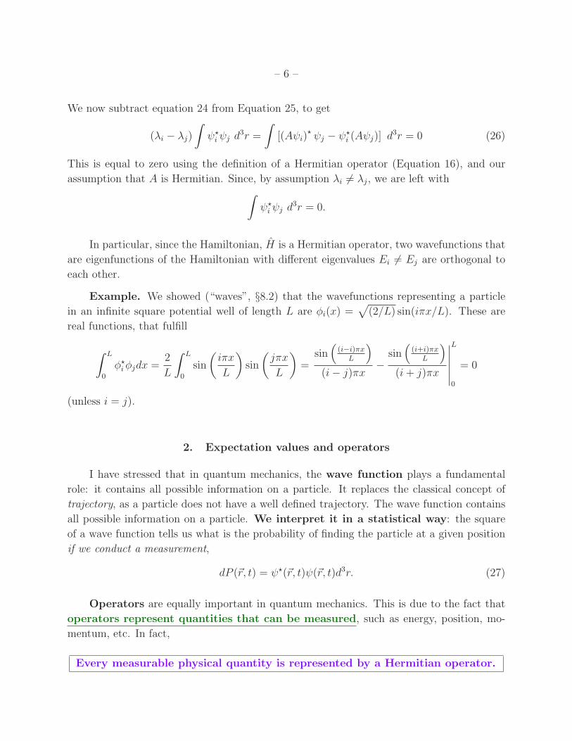
Example. We showed (“waves”, §8.2) that the wavefunctions representing a particle

in an infinite square potential well of length L are φi(x) =√

(2/L) sin(iπx/L). These are

real functions, that fulfill

∫ L

0

φ⋆iφjdx =2

L

∫ L

0

sin

(

iπx

L

)

sin

(

jπx

L

)

=sin

(

(i−i)πxL

)

(i− j)πx−

sin(

(i+i)πxL

)

(i+ j)πx

∣

∣

∣

∣

∣

∣

L

0

= 0

(unless i = j).

2. Expectation values and operators

I have stressed that in quantum mechanics, the wave function plays a fundamental

role: it contains all possible information on a particle. It replaces the classical concept of

trajectory, as a particle does not have a well defined trajectory. The wave function contains

all possible information on a particle. We interpret it in a statistical way: the square

of a wave function tells us what is the probability of finding the particle at a given position

if we conduct a measurement,

dP (~r, t) = ψ⋆(~r, t)ψ(~r, t)d3r. (27)

Operators are equally important in quantum mechanics. This is due to the fact that

operators represent quantities that can be measured, such as energy, position, mo-

mentum, etc. In fact,

Every measurable physical quantity is represented by a Hermitian operator.

– 7 –

Before getting deeper into the explanation of this, let us consider a particle that is

described by a wavefunction ψ. Let us show how one can use ψ to extract information about

the particle.

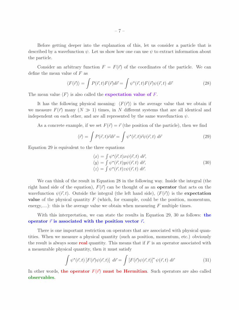
Consider an arbitrary function F = F (~r) of the coordinates of the particle. We can

define the mean value of F as

〈F (~r)〉 =

∫

P (~r, t)F (~r)d~r =

∫

ψ⋆(~r, t)F (~r)ψ(~r, t) d~r (28)

The mean value 〈F 〉 is also called the expectation value of F .

It has the following physical meaning: 〈F (~r)〉 is the average value that we obtain if

we measure F (~r) many (N ≫ 1) times, in N different systems that are all identical and

independent on each other, and are all represented by the same wavefunction ψ.

As a concrete example, if we set F (~r) = ~r (the position of the particle), then we find

〈~r〉 =

∫

P (~r, t)~rd~r =

∫

ψ⋆(~r, t)~rψ(~r, t) d~r (29)

Equation 29 is equivalent to the three equations

〈x〉 =∫

ψ⋆(~r, t)xψ(~r, t) d~r,

〈y〉 =∫

ψ⋆(~r, t)yψ(~r, t) d~r,

〈z〉 =∫

ψ⋆(~r, t)zψ(~r, t) d~r.

(30)

We can think of the result in Equation 28 in the following way. Inside the integral (the

right hand side of the equation), F (~r) can be thought of as an operator that acts on the

wavefunction ψ(~r, t). Outside the integral (the left hand side), 〈F (~r)〉 is the expectation

value of the physical quantity F (which, for example, could be the position, momentum,

energy,....): this is the average value we obtain when measuring F multiple times.

With this interpretation, we can state the results in Equation 29, 30 as follows: the

operator ~r is associated with the position vector ~r.

There is one important restriction on operators that are associated with physical quan-

tities. When we measure a physical quantity (such as position, momentum, etc.) obviously

the result is always some real quantity. This means that if F is an operator associated with

a measurable physical quantity, then it must satisfy∫

ψ⋆(~r, t) [F (~r)ψ(~r, t)] d~r =

∫

[F (~r)ψ(~r, t)]⋆ ψ(~r, t) d~r (31)

In other words, the operator F (~r) must be Hermitian. Such operators are also called

observables.

– 8 –

2.1. Functions of momentum

Often, we encounter functions not of the position of a particle, but of its momentum

- such as the momentum itself. We would like to calculate the expectation value of such a

function, G = G(~p).

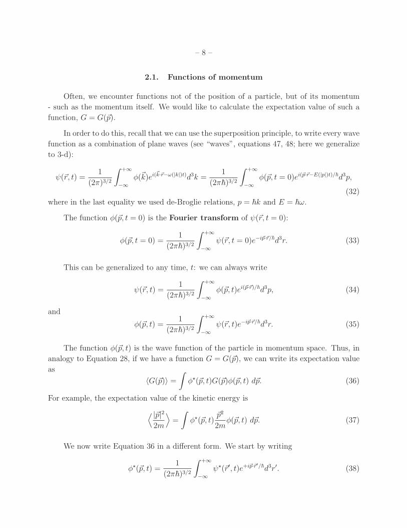
In order to do this, recall that we can use the superposition principle, to write every wave

function as a combination of plane waves (see “waves”, equations 47, 48; here we generalize

to 3-d):

ψ(~r, t) =1

(2π)3/2

∫ +∞

−∞

φ(~k)ei(~k·~r−ω(|k|)t)d3k =

1

(2π~)3/2

∫ +∞

−∞

φ(~p, t = 0)ei(~p·~r−E(|p|)t)/~d3p,

(32)

where in the last equality we used de-Broglie relations, p = ~k and E = ~ω.

The function φ(~p, t = 0) is the Fourier transform of ψ(~r, t = 0):

φ(~p, t = 0) =1

(2π~)3/2

∫ +∞

−∞

ψ(~r, t = 0)e−i~p·~r/~d3r. (33)

This can be generalized to any time, t: we can always write

ψ(~r, t) =1

(2π~)3/2

∫ +∞

−∞

φ(~p, t)ei(~p·~r)/~d3p, (34)

and

φ(~p, t) =1

(2π~)3/2

∫ +∞

−∞

ψ(~r, t)e−i~p·~r/~d3r. (35)

The function φ(~p, t) is the wave function of the particle in momentum space. Thus, in

analogy to Equation 28, if we have a function G = G(~p), we can write its expectation value

as

〈G(~p)〉 =

∫

φ⋆(~p, t)G(~p)φ(~p, t) d~p. (36)

For example, the expectation value of the kinetic energy is

⟨ |~p|2

2m

⟩

=

∫

φ⋆(~p, t)~p2

2mφ(~p, t) d~p. (37)

We now write Equation 36 in a different form. We start by writing

φ⋆(~p, t) =1

(2π~)3/2

∫ +∞

−∞

ψ⋆(~r′, t)e+i~p·~r′/~d3r′. (38)

– 9 –

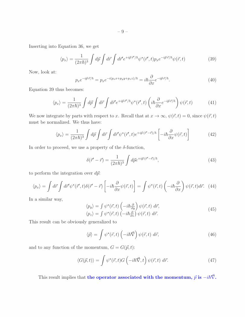
Inserting into Equation 36, we get

〈px〉 =1

(2π~)3

∫

d~p

∫

d~r

∫

d~r′e+i~p·~r′/~ψ⋆(~r′, t)pxe

−i~p·~r/~ψ(~r, t) (39)

Now, look at:

pxe−i~p·~r/~ = pxe

−i(pxx+pyy+pzz)/~ = i~∂

∂xe−i~p·~r/~. (40)

Equation 39 thus becomes:

〈px〉 =1

(2π~)3

∫

d~p

∫

d~r

∫

d~r′e+i~p·~r′/~ψ⋆(~r′, t)

(

i~∂

∂xe−i~p·~r/~

)

ψ(~r, t) (41)

We now integrate by parts with respect to x. Recall that at x→ ∞, ψ(~r, t) = 0, since ψ(~r, t)

must be normalized. We thus have:

〈px〉 =1

(2π~)3

∫

d~p

∫

d~r

∫

d~r′ψ⋆(~r′, t)e+i~p·(~r′−~r)/~

[

−i~∂

∂xψ(~r, t)

]

(42)

In order to proceed, we use a property of the δ-function,

δ(~r′ − ~r) =1

(2π~)3

∫

d~pe+i~p·(~r′−~r)/~, (43)

to perform the integration over d~p:

〈px〉 =

∫

d~r

∫

d~r′ψ⋆(~r′, t)δ(~r′ − ~r)

[

−i~∂

∂xψ(~r, t)

]

=

∫

ψ⋆(~r, t)

(

−i~∂

∂x

)

ψ(~r, t)d~r. (44)

In a similar way,

〈py〉 =∫

ψ⋆(~r, t)(

−i~ ∂∂y

)

ψ(~r, t) d~r,

〈pz〉 =∫

ψ⋆(~r, t)(

−i~ ∂∂z

)

ψ(~r, t) d~r.(45)

This result can be obviously generalized to

〈~p〉 =

∫

ψ⋆(~r, t)(

−i~~∇)

ψ(~r, t) d~r, (46)

and to any function of the momentum, G = G(~p, t):

〈G(~p, t)〉 =

∫

ψ⋆(~r, t)G(

−i~~∇, t)

ψ(~r, t) d~r. (47)

This result implies that the operator associated with the momentum, ~p is −i~~∇.

– 10 –

Example. Suppose that we want to calculate the expectation value of the total energy

of a particle that moves in a potential V (r, t). In Newtonian physics, we have E = |p|2/2m+

V (r, t). Using Equation 46, we derive the quantum mechanical analogue:

〈E〉 =

∫

ψ⋆(~r, t)

[

−~2

2m~∇2 + V (~r, t)

]

ψ(~r, t) d~r = 〈H〉 (48)

This leads to an important conclusion: the operator associated with the total energy

E of a particle is the Hamiltonian, H.

2.2. Functions of both position and momentum

We saw that the expectation values of function of the position: F = F (~r, t) or the mo-

mentum: G = G(~p, t) are always real. Hence, the operators associated with these functions

are Hermitian.

However, if we have a function of both ~r and ~p, this is not necessarily the case. For

example, consider a particle moving in 1-d, characterized by wavefunction ψ(x, t). What is

the expectation value of xpx? We have:

〈xpx〉 =

∫ +∞

−∞

ψ⋆(x, t)x

(

−i~∂

∂x

)

ψ(x, t)dx (49)

We can integrate by parts:

〈xpx〉 = −i~xψ⋆ψ|+∞−∞ + i~

∫ +∞

−∞ψ(x, t) ∂

∂x(xψ⋆(x, t)) dx

= 0 + i~∫ +∞

−∞ψx∂ψ

⋆

∂xdx+ i~

∫ +∞

−∞ψψ⋆dx

(50)

(the first term is 0, since |ψ| → 0 when x→ ±∞).

We thus find:

〈xpx〉 = 〈xpx〉⋆ + i~. (51)

The existence of the second term, i~ in Equation 51, forces us to conclude that the expec-

tation value of 〈xpx〉 cannot be real. This means that the associated operator, x(

−i~ ∂∂x

)

is

not Hermitian.

Mathematically, we just showed that the operators representing the physical quantities

of position (x) and momentum (px) do not commute. Physically, this means that we cannot

measure simultaneously both the position and momentum of a particle to infinite

precision.

– 11 –

3. Ehrenfest theorem: transition between quantum mechanics and classical

mechanics

Obviously, the above result has no classical analogue. However, we know that on a

large scale, the laws of classical mechanics do hold. Thus, there must exist conditions under

which classical mechanics provides good description of a physical system. The general rule

was formulated by Niels Bohr in 1923, and is known as the correspondence principle. A

common formulation of the principle states that the results of a quantum theory must

approach those of classical theory asymptotically in the limit of large quantum

numbers.

In order to investigate this point quantitatively and gain an insight into the nature

of quantum mechanics, we will prove the following theorem, known as Ehrenfest’s theo-

rem. Consider Newton’s laws, written in the following form, known as Hamilton-Jacobi

equations (yes, the same Hamilton from the Hamiltonian):

d~rdt

= ~pm;

d~pdt

= −~∇V.(52)

Clearly, these are classical equations of motion.

Ehrenfest’s theorem states that the same equations are satisfied by the expecta-

tion values (=average values) of the corresponding quantum mechanics opera-

tors. Note an important point. In quantum mechanics, there are no well-define trajectories,

as in classical mechanics, so in this sense terms such as d~r/dt which gives the change in

direction along a classical path does not exist. However, the expectation values of operators

such as ~r do change with time, and so it does make sense to look at their temporal evolution.

In the mathematical proof, we will use Green’s identities from vector calculus. Green’s

first identity states that if u and v are two scalar functions of the position (u = u(x, y, z),

v = v(x, , z)), both have continuous first and second derivatives, then

∫

V

[

u∇2v + (∇u) · (∇v)]

d3r =

∫

S

u(∇v) · dS, (53)

where S is the surface enclosing the volume V . Green’s second identity states that for these

functions,∫

V

[

u(∇2v)− v(∇2u)]

d3r =

∫

S

[u(∇v)− v(∇u)] · dS. (54)

(These theorems can be viewed as special cases of the divergence theorem,∫

V(~∇ · ~F )dV =

∮

~F · d~S).

– 12 –

proof. Using Equation 30, we have

ddt〈x〉 = d

dt

∫

ψ⋆(~r, t)xψ(~r, t) d~r

=∫

ψ⋆(~r, t)xdψ(~r,t)dt

d~r +∫ dψ⋆(~r,t)

dtxψ(~r, t) d~r

(55)

Using Schrodinger equation and its complex conjugate (Equations 13, 14), we have

ddt〈x〉 = 1

i~

[

∫

ψ⋆x(Hψ) d~r −∫

(Hψ)⋆xψ d~r]

= i~2m

∫

[ψ⋆x(∇2ψ)− (∇2ψ⋆)xψ] d~r.(56)

(The terms involve the potential V cancel out).

We now use Green’s first identity, setting u = xψ and v = ψ⋆ to write the second integral:

∫

(∇2ψ⋆)xψ d~r =

∫

S

xψ(∇ψ⋆) · dS −

∫

(∇ψ⋆) · (∇xψ) d~r = −

∫

(∇ψ⋆) · (∇xψ) d~r (57)

(the first integral over dS must be equal to zero, since the surface encloses all space, and

ψ → 0 at |~r| → ∞).

We use again Green’s first identity, to write

−

∫

(∇ψ⋆) · (∇xψ) d~r = −

∫

S

ψ⋆∇(xψ) · dS +

∫

ψ⋆∇2(xψ) d~r =

∫

ψ⋆∇2(xψ) d~r (58)

(from the same reasoning).

Putting this in Equation 56, we find

d

dt〈x〉 =

i~

2m

∫

ψ⋆[

x(∇2ψ)−∇2(xψ)]

d~r = −i~

m

∫

ψ⋆∂ψ

∂xd~r (59)

where the last equality comes from expansion of the second term.

Comparing this result to Equation 44, one finds

d

dt〈x〉 =

〈px〉

m, (60)

which is the quantum mechanical counterpart of the first of the classical Hamilton-Jacobi

Equations (Equation 52).

The second part of Ehrenfest’s theorem is proven in a similar way. From the expectation

value of the momentum (Equation 44 we have

d

dt〈px〉 = −i~

d

dt

∫

ψ⋆∂ψ

∂xd~r = −i~

[∫

ψ⋆∂

∂x

∂ψ

∂td~r +

∫

∂ψ⋆

∂t

∂ψ

∂xd~r

]

(61)

– 13 –

Using Schrodinger equation and its complex conjugate to re-write ∂ψ/∂t and ∂ψ⋆/∂t, one

obtains

ddt〈px〉 = −

∫

ψ⋆ ∂∂x

(

− ~2

2m∇2ψ + V ψ

)

d~r +∫

(

− ~2

2m∇2ψ⋆ + V ψ⋆

)

∂ψ∂x

d~r

= ~2

2m

∫ [

ψ⋆(

∇2 ∂ψ∂x

)

− (∇2ψ⋆)∂ψ∂x

]

d~r −∫

ψ⋆[

∂∂x(V ψ)− V ∂ψ

∂x

]

d~r(62)

Assuming that ψ and ∂ψ/∂x vanish at large x, the first integral vanishes by Green’s second

identity (using u = ψ⋆ and v = ∂ψ/∂x). The second integral is

−

∫

ψ⋆[

∂

∂x(V ψ)− V

∂ψ

∂x

]

d~r = −

∫

ψ⋆∂V

∂xψ d~r = −

⟨∂V

∂x

⟩

. (63)

We thus found thatd

dt〈px〉 = −

⟨∂V

∂x

⟩

(64)

which completes the proof.

Physical meaning. Let us assume that the wave function ψ that describes the particle

takes the form of a wavepacket. We can therefore consider the average value (=expectation

value) 〈~r〉(t) to be the center of the wavepacket at time t. Thus, the set of all points 〈~r〉(t)

corresponding to different times form a trajectory: this is the trajectory followed by the

center of the wave packet.

The conclusion is, that although we cannot speak of a trajectory of the particle itself

(since ψ extends over all space), we can speak of a trajectory of the center of the wave

packet. If all the distances involved in the problem are much bigger than the extension of

the wave packet, we can approximate the wave packet by its center, and recover the classical

description of trajectory, and the classical results.

4. Dirac’s bracket notation

We saw that in quantum mechanics, the quantum state of a particle is fully specified

by a wave function, ψ(~r, t). On the other hand, not every wave function can describe a

physical particle: a wave function must be square integrable and normalized, in order for it

to describe a physical particle:∫

|ψ(~r, t)|2 d3r = 1. (65)

From a physical point of view, we add a few requirements: these functions must be every-

where defined, continuous, and infinitely differentiable.

Technically, the set of functions ψ for which the integral converges, form what is called

by mathematicians L2 space. This space has all the properties of a vector space, which we

– 14 –

will not go into in full details here. However, I do point into two important aspects of it:

(i) the superposition principle, according to which if ψ1 and ψ2 belong to this space, so

will

ψ(~r) = λ1ψ1(~r) + λ2ψ2(~r),

where λ1 and λ2 are two arbitrary complex numbers; and

(ii) the ability to define a scalar product between two functions, φ(~r) and ψ(~r, t) using

∫

φ⋆(~r, t)ψ(~r, t) d3r.

For those who are familiar with the mathematical definitions, we say that L2 is an example

of an infinite-dimensions Hilbert space.

This association of wave functions as elements in a vector space, enable us to use a

convenient notation, according to Paul Dirac. To each wave function, ψ(~r), we associate a

ket vector, or simply ket, which we denote by |ψ〉. Thus:

ψ(~r) ⇐⇒ |ψ〉 (66)

The set of ket vectors, also known as state vectors of a quantum system, define a space.

It is known as the “state space” of the system. (Technically, this space is isomorphic to the

space defined by the functions ψ(~r), but we do not need to get into the mathematical details

of this). Note that we generalize |ψ〉 to describe the state of a quantum system, which may

include more than a single particle.

We omit the ~r dependence from |ψ〉. In fact (we will not prove it here), we could think of

ψ(~r) as the components of the ket |ψ〉 in a particular basis, ~r. However, this goes somewhat

deeper than currently needed.

One point which is important to remember, is that the use of Dirac’s notation enables

not only to simplify the calculations, but also to generalize them. There exist physical

systems whose quantum description cannot be fully given by a wave function. A classical

example is the spin degree of freedom (which we may or may not have time to cover this

year). Nonetheless, such systems can still be described by specifying their state vector.

4.1. Bras and Scalar product

To each ket vector, |ψ〉, there is an associated bra vector, or simply bra, denoted by 〈ψ|.

Technically, the bra can be thought of a linear functional. A linear functional is a linear

operation that associates with every ket |ψ〉 a complex number. This is done in a linear way.

– 15 –

Note the difference between a linear functional that associates with every ket a number, and

a linear operator discussed above, that associates with every ket another ket. For those who

are familiar with the term, we say that 〈ψ| belongs to the dual space of the vector space

defined by the kets.

With each pair of bra 〈φ| and ket |ψ〉, taken in this order, we can therefore associate

a complex number - which is their scalar product, defined by

〈φ|ψ〉 ≡

∫

φ⋆(~r)ψ(~r) d3r. (67)

It is obvious from this definition that

〈φ|ψ〉 = 〈ψ|φ〉⋆. (68)

Furthermore, if λ is a complex number, we obviously have

〈φ|λψ〉 = λ〈φ|ψ〉

〈λφ|ψ〉 = λ⋆〈φ|ψ〉

〈φ|ψ1 + ψ2〉 = 〈φ|ψ1〉+ 〈φ|ψ2〉

(69)

Using this Dirac notation, the normalization condition of the wavefunction (Equation 65)

can be written in a compact form,

〈ψ|ψ〉 = 1. (70)

Furthermore, the functions ψ and φ are said to be orthogonal, if their scalar product vanishes:

〈φ|ψ〉 = 0. (71)

5. Linear operators (part II)

We saw that a linear operator A associates with every wavefunction ψ another wavefunc-

tion ψ = Aψ, in a linear way, namely A(λ1ψ1 + λ2ψ2) = λ1(Aψ1) + λ2(Aψ2) (see Equations

4, 5). Using Dirac’s notation, we write

|ψ〉 = A|ψ〉,

A(λ1|ψ1〉+ λ2|ψ2〉) = λ1A|ψ1〉+ λ2A|ψ2〉.(72)

Using Equations 67 and 72, we know that 〈φ|ψ〉 = 〈φ|(A|ψ〉) is a complex number. Since

both the scalar product and the operator A are linear, this complex number depends linearly

– 16 –

on |ψ〉. We can therefore think of both 〈φ| and A as defining a new bra, that associates with

each ket |ψ〉 a complex number; in other words, we can write

(〈φ|A)|ψ〉 = 〈φ|(A|ψ〉) ≡ 〈φ|A|ψ〉 (73)

where we omitted the parenthesis, as their place is unimportant. This is known as the

matrix element between the kets |φ〉 and |ψ〉 (obviously, |φ〉 is the ket associated with the

bra 〈φ|).

Example: the projection operator.

Let |ψ〉 be a ket which is normalized to one:

〈ψ|ψ〉 = 1.

Consider the operator Pψ defined by:

Pψ = |ψ〉〈ψ| (74)

apply it to arbitrary ket, |φ〉:

Pψ|φ〉 = |ψ〉〈ψ|φ〉 (75)

We see that we obtain a ket which is proportional to |ψ〉; the coefficient of proportionality,

〈ψ|φ〉 is a complex number, which is the scalar product of 〈ψ| and |φ〉. This has an obvious

“geometrical” interpretation.

Furthermore, we have

P 2ψ = PψPψ = |ψ〉〈ψ|ψ〉〈ψ| = |ψ〉〈ψ| = Pψ, (76)

where we used the fact that 〈ψ|ψ〉 = 1.

5.1. Adjoint operators

The association between kets and bras enable to associate with each linear operator

A, another linear operator, called the adjoint operator, that is denoted by A†. Another

name for adjoint operators is Hermitian conjugates (not to be confused with Hermitian

operators!).

Let |ψ〉 be an arbitrary ket. The operator A associates with it another ket, |ψ〉. Now,

let 〈ψ| be the bra associated with |ψ〉 , and 〈ψ| the bra associated with the ket |ψ〉. The

bra-ket correspondence, enable us to define the operator A† that acts on the bras:

〈ψ| = 〈ψ|A† ⇐⇒ A|ψ〉 = |ψ〉. (77)

– 17 –

Using the property of the scalar product (equation 68), 〈ψ|φ〉 = 〈φ|ψ〉⋆, we can write

〈ψ|A†|φ〉 = 〈φ|A|ψ〉⋆ (78)

(note that both sides of Equation 78 are c-numbers !). This is valid for all 〈φ| and |ψ〉. The

operator A† is known as the Hermitian conjugate of the operator A.

The concept of adjoint operators can be understood as operator generalization of the

the complex conjugate of a complex number.

It is straight forward to show that

(A†)† = A

(λA)† = λ⋆A†

(A+ B)† = A† +B†

(79)

By applying two operators once at a time, one can also show that

(AB)† = B†A† (80)

5.2. Hermitian operators (again)

If a linear operator A satisfies

A† = A (81)

then it is called self adjoint. In this case, Equation 78 becomes

〈ψ|A|φ〉 = 〈φ|A|ψ〉⋆ (82)

Comparing this to Equation 16, we see that this is similar to the definition of a Hermitian

operator (identical if |φ〉 = |ψ〉). In fact, it is not difficult to show that the two definitions

are equivalent. Thus, self-adjoint is another name to Hermitian operator.

Alternatively, we could define Hermitian operator A by

〈φ|(Aψ)〉 = 〈(Aφ)|ψ〉 (83)

where we used the notation |(Aψ)〉 ≡ A|ψ〉 and 〈(Aψ)| = 〈ψ|A†.

We can now repeat the discussion above about the properties of the eigenfunctions

and eigenvalues of Hermitian operators, using Dirac’s notation. For example, if ψn is an

eigenfunction of the operator A with eigenvalue an, then from Aψn = anψn we have

〈ψn|A|ψn〉 = an〈ψn|ψn〉 (84)

– 18 –

and since (Aψn)⋆ = a⋆nψ

⋆n, we have

〈(Aψn)|ψn〉 = a⋆n〈ψn|ψn〉. (85)

If A is Hermitian, the left hand sides of Equations 84, 85 are equal, hence an = a⋆n, namely

the eigenvalues of A are real.

Similarly, we can prove the orthogonality properties of the eigenfunctions of A. If ψiand ψj are eigenfunctions of A with two different eigenvalues, ai and aj, we have Aψi = aiψiand Aψj = ajψj. Thus,

(ai − aj)〈ψi|ψj〉 = 〈aiψi|ψj〉 − 〈ψi|ajψj〉 = 〈(Aψi)|ψj〉 − 〈ψi|(Aψj)〉 = 0 (86)

where we have used the fact that A is Hermitian. Since ai 6= aj, it follows immediately that

〈ψi|ψj〉 = 0 (i 6= j).

Furthermore, if ψn is an eigenfunction of the operator A, its corresponding ket, |ψn〉 is

called eigenvector of A.

5.3. Physical interpretation: observables

A basic postulate of quantum mechanics is that

Every measurable physical quantity (position, energy, momen-

tum, etc.) is described by a Hermitian operator, A. This oper-

ator is an observable.

Now, if the wavefunction of a system happens to be an eigenfunction ψn of the operator A

(corresponding eigenvalue an), then (second postulate): a measurement of the dynamical

variable A will certainly produce the result an. We say that the system is in an

eigenstate of A characterized by eigenvalue an. The set of all eigenvalues of A are

called the spectrum of A.

If, on the other hand, the wave function ψ describing the system is not an eigenfunction

of A, then, when measuring A, any one of the results a1, a2, ..can be obtained. We don’t

know in advanced which result will be obtained; but we can calculate the probability of

obtaining a certain result (we will show shortly how).

If the system is described by wavefunction ψ that is normalized, namely 〈ψ|ψ〉 = 1,

– 19 –

then in analogy to the discussion above, we define the expectation value of A as

〈A〉 ≡ 〈ψ|A|ψ〉.1 (87)

5.4. Functions of operators

Consider an arbitrary operator A. One can easily define the operator An: this is the

operator which corresponds to n successive applications of the operator A: An|ψ〉 = A · A ·

.... · A|ψ〉. But what about a general function of operator, f(A) ?

In analogy to power series expansion of functions of a variable, z: f(z) =∑∞

i=0 cizi, we

can define the operator function f(A) as

f(A) ≡∞∑

i=0

ciAi (88)

Consequently, if |ψn〉 is one of the eigenfunctions of A corresponding to the eigenvalue an,

we have: Ai|ψn〉 = (an)i|ψn〉. Thus,

f(A)|ψn〉 = f(an)|ψn〉. (89)

In words: we just proved that if |ψn〉 is an eigenvector of A with the eigenvalue an, then |ψn〉

is also an eigenvector of f(A) with the eigenvalue f(an).

This leads to another insight. As we will immediately show, operators are best rep-

resented by matrices, once we specify a set of basis vectors. If we find a basis such that

the matrix representing an operator A is diagonal (namely, zero everywhere except from the

diagonal) - which is something that we can always do for an observable - then the matrix

representing f(A), in the same basis, is also diagonal, whose elements are f(a).

Example. The operator eA is defined be

eA ≡∞∑

n=0

An

n!= I + A+

A2

2!+ ...+

An

n!+ .... (90)

Note that as opposed to numbers, in general, f(A)f(B) 6= f(B)f(A), unless the operators A

and B commute. In fact, one can show that eAeB = eA+Be1

2[A,B]. This is known as Glauber’s

formula.

1If the wavefunction ψ is not normalized, we define the expectation value of A as 〈A〉 ≡ 〈ψ|A|ψ〉〈ψ|psi〉 .

– 20 –

This example is particularly useful when solving the Schrodinger equation, i~ ∂∂t|ψ(t)〉 =

H|ψ(t)〉. For a time-independent Hamiltonian, the solution to this equation is

|ψ(t)〉 = e−iHt

~ |ψ(t = 0)〉,

and so the state vector at arbitrary time |ψ(t)〉 can be immediately calculated if |ψ(t = 0)〉

(the state of the system at t = 0) is known and the Hamiltonian can be written in the form

of a diagonal matrix, as is frequently the case.

Example - 2. The operator σz (known as one of Pauli’s spin matrices) is represented

by the matrix

σZ =

(

1 0

0 −1

)

(91)

It follows directly that

eσZ =

(

e 0

0 1/e

)

. (92)

6. Representations in state space

We stated that for each wavefunction ψ there corresponds a ket vector, |ψ〉 in the “state

space” of the system. In order to calculate the expectation values of the different observables

(as well as other calculations), we need first to define an orthonormal basis for this space

(namely, all the basis vectors are normalized to unity, and are orthogonal to each other).

This basis can be either discrete, or continuous, depending on the spectrum (=all possible

results of measurements) of the particular observable.

Once we specify a basis, vectors and operators are represented by numbers: for vectors,

these are their components in the given basis (exactly the same way as we represent vectors by

their x, y and z components in Cartesian coordinate system). Operators will be represented

by their matrix elements. In theory, the choice of representation is arbitrary. Practically, we

obviously choose a representation which simplifies the calculations as much as possible.

Let us discriminate between the two cases: discrete and continuous basis. (To avoid

confusion, I am omitting discussion on degeneracy).

– 21 –

6.1. Discrete basis

A set of discrete kets, {|ψi〉} is said to be orthonormal, if the kets of this set satisfy

the orthonormalization condition:

〈ψi|ψj〉 = δij (93)

where δij is the Kronecker delta symbol,

δij =

{

1, i = j

0, i 6= j.(94)

In order for the set {|ψi〉} to form a basis, every wavefunction must have a unique

expansion on the |ψi〉, namely every wavefunction can be expressed as a linear combination

of |ψi〉:

|Ψ〉 =∑

i

ci|ψi〉 (95)

Since this must be true for all wave functions, the set |ψi〉 is said to be complete.

We can multiply both sides of Equation 95 by 〈ψj|, to get

〈ψj|Ψ〉 = cj (96)

Using this in Equation 95, one obtains:

|Ψ〉 =∑

i

(〈ψi|Ψ〉) |ψi〉 =∑

i

|ψi〉〈ψi|Ψ〉 (97)

We can think of∑

i |ψi〉〈ψi| as an operator, that when acting on any arbitrary ket |Ψ〉 gives

the same ket; thus,∑

i

|ψi〉〈ψi| = I (98)

where I denotes the identity operator. Equation 98 is also known as the closure relation,

as it expresses the completeness of the set of functions {|ψi〉}.

Probability amplitude.

Consider a system that is described by a wavefunction Ψ, which is normalized to unity. Let

{ψn} be a complete set of eigenfunctions of A, whose corresponding kets {|ψn〉} form an

orthonormal basis.

The expectation value of an (arbitrary) observable A is given by Equation 87,

〈A〉 ≡ 〈Ψ|A|Ψ〉

=∑

m

∑

n c⋆mcn〈ψm|A|ψn〉

=∑

m

∑

n c⋆mcnan〈ψm|ψn〉

=∑

n |cn|2an

(99)

– 22 –

Since Ψ is normalized to unity, 〈Ψ|Ψ〉 = 1 namely∑

n |cn|2 = 1.

Now, recall the following: when we measure A, the only possible results that we can

obtain are an. When we measure A multiple times (in a large number of identical systems),

the average value we obtain is 〈A〉. Thus, we interpret the quantity

Pn = |cn|2 = |〈ψn|Ψ〉|2 (100)

as the probability of obtaining the particular value an in a given measurement. The coefficients

cn = 〈ψn|Ψ〉 are called probability amplitudes.

Let us consider a scenario in which the state of a system, |Ψ〉 is known, and we want to

measure an observable A. Before the measurement, we don’t know what value we will get; we

only know the probability amplitude of obtaining the various possible values. Suppose now

we actually measure A, and obtained a value an. Immediately after the measurement,

we obviously cannot speak of “probability of obtaining a value”; the value is known. Thus,

clearly, the state of the system is no longer |Ψ〉. Instead,

The state of the system immediately after the measurement is

the eigenvector |ψn〉 associated with an.

6.2. Continuous spectrum

The spectrum of some observables, e.g., the momentum operator px is continuous, while

the spectrum of others, e.g., the Hamiltonian, possess both a discrete and continuous part.

We thus need to generalize the treatment in the previous section to these cases.

The treatment is very similar to the discrete case. Let us denote the set of continuous

eigenvalues by a, and eigenfunctions by ψa, namely Aψa = aψa. We can write any arbitrary

wave function Ψ as

Ψ =

∫

c(a)ψada, (101)

where the integral runs over all values of a. Alternatively, we could write |Ψ〉 =∫

da c(a)|ψa〉.

The set of eigenfunctions must be orthonormal, namely

〈ψa′ |ψa〉 = δ(a− a′), (102)

(compare to Equation 93), enabling us to write the coefficients a(a) as

c(a) = 〈ψa|Ψ〉 (103)

– 23 –

(compare to Equation 96).

The closure relation takes the form∫

da|ψa〉〈ψa| = I. (104)

The expectation value of an operator is written as

〈A〉 ≡ 〈Ψ|A|Ψ〉

=∫

da∫

da′c⋆(a′)c(a)〈ψa′|A|ψa〉

=∫

da∫

da′c⋆(a′)c(a)a〈ψa′|ψa〉

=∫

da|c(a)|2a

(105)

6.3. Matrix representation of wave functions and operators

6.3.1. Representation of kets

Let us assume that {|ψi〉} form a complete set of orthonormal basis (for simplicity, I

consider only the discrete case here). As we saw, this means that every wave function can

be written as

|Ψ〉 =∑

i

ci|ψi〉

(see Equation 95). Therefore, once we know the set {|ψi〉}, the set of coefficients ci = 〈ψi|Ψ〉

fully determines |Ψ〉. It is analogous to the way we describe a vector (in 3-d space) by its x,

y and z components, which we can specify after we define the coordinate system.

Thus, we can think of the set of functions {|ψi〉} as analogue to the set of orthogonal

axes, and ci as analogue to the components of the ’vector’ Ψ along each of these axes. We

can arrange the ci vertically, in a column vector = one column matrix (it can, in principle,

be of infinite length!)

c1c2...

cn...

=

〈ψ1|Ψ〉

〈ψ2|Ψ〉...

〈ψn|Ψ〉...

(106)

– 24 –

6.3.2. Representation of bras and scalar product

Similar to kets, every bra 〈Ψ| has a unique representation in the orthonormal (bra) basis

{〈ψi|}. Using the closure relation (Equation 98), we can write

〈Ψ| = 〈Ψ|I =∑

i

〈Ψ|ψi〉〈ψi| (107)

Obviously, the components of 〈Ψ|, namely 〈Ψ|ψi〉 are the complex conjugates of the compo-

nents of the ket |Ψ〉 associated with the bra 〈Ψ| (see Equation 67), and are therefore equal

to c⋆i .

We thus arrange the components of the bra 〈Ψ| horizontally, forming a row vector,

(〈Ψ|ψ1〉, 〈Ψ|ψ2〉, ....〈Ψ|ψn〉) (108)

We can now look again at the scalar product (Equation 67). We can use the closure

relation (Equation 98) to write

〈φ|Ψ〉 = 〈φ|I|Ψ〉 =∑

i

〈φ|ψi〉〈ψi|Ψ〉 =∑

i

b⋆i ci (109)

where we wrote b⋆i ≡ 〈φ|ψi〉.

Not surprising at all, this is exactly what we get when we multiply the row vector

representing 〈φ| (Equation 108) with the column vector representing |Ψ〉 (Equation 106)!

6.3.3. Matrix representation of operators

Given a linear operator A, we can, in the {|ψi〉} basis associate with it a series of

numbers defined by

Aij = 〈ψi|A|ψj〉. (110)

These numbers are called the matrix elements of the operator A in the basis {|ψi〉}.

As these numbers depend on two indices, we can therefore arrange them in a matrix

form:

A11 A12 . . . A1j . . .

A21 A22 . . . A2j . . ....

......

Ai1 Ai2 . . . Aij . . ....

......

(111)

– 25 –

The operator A, when acting on the ket |Ψ〉 produces a new ket,

|Φ〉 = A|Ψ〉.

If we know the representation of the ket |Ψ〉 (namely, its components in the basis {|ψi〉} )

and the matrix representation of A in the the same basis, we can calculate the components

of |Φ〉 using

bi = 〈ψi|Φ〉 = 〈ψi|A|Ψ〉 =∑

j

〈ψi|A|ψj〉〈ψj|Ψ〉 =∑

j

Aijcj (112)

where we made use of the closure relation (Equation 98).

This equation can also be written as a matrix equation, using the standard formula for

matrix multiplication:

b1b2...

bi...

=

A11 A12 . . . A1j . . .

A21 A22 . . . A2j . . ....

......

Ai1 Ai2 . . . Aij . . ....

......

c1c2......

cj

(113)

Using this representation the matrix representation of the operator C which is obtained

by the product of two operators, C = AB is simply the matrix product of the two matrices

representing the operators A and B. This can be verified by using again the closure relation

(equation 98):

Cij = 〈ψi|C|ψj〉 = 〈ψi|AB|ψj〉 =∑

k

〈ψi|A|ψk〉〈ψk|B|ψj〉 =∑

k

AikBkj (114)

Matrix representation of adjoint operators.

Using Equation 78 (〈ψ|A†|φ〉 = 〈φ|A|ψ〉⋆), we find:

(A†)ij = 〈ψi|A†|ψj〉 = 〈ψj|A|ψi〉

⋆ = A⋆ji (115)

Therefore, the matrix elements of A† are obtained from the matrix elements of A

by interchanging rows and columns and then taking the complex conjugate of

each element. (And vice versa, of course).

If A is Hermitian, then we have A† = A; therefore, (A†)ij = Aij and therefore

Aij = A⋆ji (116)

– 26 –

Such a matrix is called Hermitian matrix. Namely, a Hermitian operator is represented

by a matrix in which any two elements which are symmetric with respect to the

principle diagonal are complex conjugates of each other.

In particular, all the elements on the diagonal, Aii must have Aii = A⋆ii, namely, the

diagonal elements of a Hermitian matrix are always real numbers.

6.4. Finding eigenvalues and eigenvectors of an operator

Clearly, we say that |Ψ〉 is an eigenvector (or eigenket) of the operator A with eigenvalue

λ if

A|Ψ〉 = λ|Ψ〉. (117)

We would like to answer the following question: given an operator A, how do we find all its

eigenvalues and the corresponding eigenvectors ?

Let us assume that {|ψi〉} forms a basis in some particular representation. We can then

project the vector Equation 117 onto the various orthonormal basis vectors,

〈ψi|A|Ψ〉 = λ〈ψi|Ψ〉 (118)

Inserting the closure relation between A and |Ψ〉 gives∑

j

〈ψi|A|ψj〉〈ψj|Ψ〉 = λ〈ψi|Ψ〉 (119)

Using Equations 96 (〈ψj|Ψ〉 = cj) and 110 (Aij = 〈ψi|A|ψj〉), this becomes

∑

j

Aijcj = λci, (120)

or∑

j

[Aij − λδij] cj = 0. (121)

This equation can be thought of a linear and homogeneous system of N equations, in N

unknowns (cj). From linear algebra, we know that non-trivial solution (namely, a solution

in which not all cj = 0) exists if and only if the determinant

Det[A− λI] = 0, (122)

where A is the (N ×N) matrix of the Aij and I is the unit matrix. Equation 122 is known

as the characteristic equation (also: secular equation). The eigenvalues of the operator

are the roots of its characteristic equation.

– 27 –

Once we solve the equation and find the eigenvalues, we can find the eigenvectors. Let

us assume that λ0 is an eigenvalue that solves the set of N equations. When we put λ = λ0in equation 120, we are left with N − 1 independent equations, but with N unknowns (cj).

Thus, we need to fix, say c1, and the rest will depend on this choice, namely cj = αjc1 for

j 6= 1. (Obviously, for, j = 1, α1 = 1). We obtain as the eigenket, |ψ(c1)〉 =∑

j αjc1|ψj〉.

7. Commuting observables, compatibility and the Heisenberg uncertainty

relation

Consider two operators A and B. We defined earlier (see Equation 6) their commutator

by

[A,B] ≡ AB −BA.

If the commutator vanishes when acting on any wave function ψ, then the two operators A

and B are said to commute, namely AB = BA.

Assume now that A and B are two observables. If there exists a complete set of wave-

functions ψn such that each function is simultaneously an eigenfunction of both A and B,

the observables A and B are said to be compatible. Denote by an and bn the eigenvalues

of A and B corresponding to the eigenkets |ψn〉:

A|ψn〉 = an|ψn〉, B|ψn〉 = bn|ψn〉. (123)

If a state is described by |ψn〉, a measurement of A produces an exact result an, and a

measurement of B produces an exact result bn - both accurate to any precision.

Examples of compatible observers are the Cartesian components, x y and z of the posi-

tion vector ~r of a particle. Another example are the Cartesian components of its momentum,

px, py and pz. However, recall that x and px are not compatible (see Equation 51).

Two compatible observables commute. If |ψn〉 is a common eigenket, we have

AB|ψn〉 = anbn|ψn〉 = bnan|ψn〉 = BA|ψn〉 (124)

Since any ket can be expanded as |Ψ〉 =∑

n cn|ψn〉 (see Equation 95), we have

(AB −BA)|Ψ〉 =∑

n

cn(AB − BA)|ψn〉 = 0, (125)

from which it is obvious that [A,B] = 0.

– 28 –

The opposite statement, namely that two observables which commute possess a complete

set of common eigenfunctions is also true.2 Assume that |ψn〉 is an eigenket of A with

eigenvalue an. If A and B commute, we have

A(B|ψn〉) = BA|ψn〉 = an(B|ψn〉) (126)

Thus, the ket (B|ψn〉) is an eigenket of A with eigenvalue an. By assumption, an is non-

degenerate, and so (B|ψn〉) can only differ from |ψn〉 by a constant, which we call bn, namely

B|ψn〉 = bn|ψn〉 (127)

We thus see that |ψn〉 is simultaneously an eigenket of the operators A and B, with the

corresponding eigenvalues an and bn.

7.1. Heisenberg uncertainty relation

We are now at a stage to obtain a precise form of Heisenberg’s uncertainty relation.

Consider two observables, A and B, whose expectation values are 〈A〉 ≡ 〈Ψ|A|Ψ〉 and

〈B〉 ≡ 〈Ψ|B|Ψ〉 when the system is in state |Ψ〉 (see Equation 87).

We define the uncertainty ∆A to be

(∆A)2 ≡ 〈(A− 〈A〉)2〉 = 〈A2〉 − 〈A〉2 (128)

and a similar definition of ∆B.

We shall now prove the mathematical formula:

∆A ·∆B ≥1

2|〈[A,B]〉| (129)

Proof. Consider the operators

A ≡ A− 〈A〉, B ≡ B − 〈B〉.

The expectation values of both these operators vanish, 〈A〉 = 〈B〉 = 0. We further have

〈A2〉 = 〈A2〉 − 〈A〉2 = (∆A)2 (130)

2I prove this statement here only for the non-degenerate case.

– 29 –

Furthermore,

[A, B] = [A− 〈A〉, B − 〈B〉] = [A,B] (131)

since the expectation values are just numbers.

Consider now the linear (non-Hermitian) operator

C = A+ iλB, (132)

where λ is a real constant. The adjoint operator is C† = A− iλB (recall that both A and B

are Hermitian), and thus the expectation value of CC† is real and non-negative, since

〈CC†〉 = 〈Ψ|CC†|Ψ〉 = 〈C†Ψ|C†Ψ〉 ≥ 0. (133)

We thus deduce that the expectation value of

〈(A+ iλB)(A− iλB)〉 = 〈A2 + λ2B2 − iλ[A, B]〉 (134)

is both real and non-negative. Using Equations 134, 130 and 131, this means that the

function

f(λ) = 〈A2〉+ λ2〈B2〉 − iλ〈[A, B]〉 = (∆A)2 + λ2(∆B)2 − iλ〈[A,B]〉 (135)

is also real and non-negative. Therefore, 〈[A,B]〉 must be purely imaginary.

Be differentiating with respect to λ, one finds the minimum of f(λ) to be given for

λ = λ0 =i

2

〈[A,B]〉

(∆B)2. (136)

At λ = λ0, the value of f(λ) is

f(λ0) = (∆A)2 +1

4

(〈[A,B]〉)2

(∆B)2. (137)

Since we know that f(λ0) ≥ 0, we find that

(∆A)2(∆B)2 ≥ −1

4(〈[A,B]〉)2. (138)

Finally, since 〈[A,B]〉 is purely imaginary, Equation 129

∆A ·∆B ≥1

2|〈[A,B]〉|

follows, which completes the proof.

– 30 –

Example. For two observables for which [A,B] = i~, we have 〈[A,B]〉 = i~ and we

therefore deduce

∆A∆B ≥~

2(139)

Specifically, we have

∆x∆px ≥~

2, ∆y∆py ≥

~

2, ∆z∆pz ≥

~

2. (140)

where ∆x = [〈(x− 〈x〉)2〉]1/2, ∆px = [〈(px − 〈px〉)2〉]1/2, etc.

8. Summary: basic postulates of quantum mechanics

Let us summarize the basic principles and postulates of quantum mechanics.

1. The state of a system is completely specified by a wave function ψ, or state

vector, |ψ〉, which contain all the information that can be known about the

system. This function is, in general, complex. The interpretation of this

wave function is probabilistic.

2. Every measurable physical quantity is described by a Hermitian operator

A. The operator is called an observable.

3. The only possible result of a precise measurement of a physical quantity is

one of the eigenvalues of the corresponding observable A.

4. In a series of measurements of a variable A made in an ensemble of sys-

tems all having normalized state function |Ψ〉, the expectation value of this

variable is

〈A〉 = 〈Ψ|A|Ψ〉.

The probability of obtaining the (non-degenerated) eigenvalue an is

P (an) = |〈ψn|Ψ〉|2,

where |ψn〉 is the normalized eigenvector of A associated with the eigenvalue

an.

5. (Completeness): Any wavefunction can be expressed as a linear combina-

tion of the eigenfunctions of A, where A is an operator associated with a

dynamical variable (i.e., an observable).

– 31 –

6. The temporal evolution of a state vector |ψ〉 is governed by the Schrodinger equa-

tion,

i~d

dt|ψ(t)〉 = H(t)|ψ〉

where H is the Hamiltonian operator, which is the observable associated

with the total energy of the system.

Using Schrodinger equation, we can calculate the temporal evolution of the expectation

value of an operator. We have

ddt〈A〉 = d

dt〈Ψ|A|Ψ〉 =

⟨

∂Ψ∂t|A|Ψ

⟩

+⟨

Ψ|∂A∂t|Ψ

⟩

+⟨

Ψ|A|∂Ψ∂t

⟩

= − 1i~〈HΨ|A|Ψ〉+

⟨

Ψ|∂A∂t|Ψ

⟩

+ 1i~〈Ψ|A|HΨ〉

= 1i~〈[A, H]〉+

⟨

∂A∂t

⟩

(141)

In particular, if the operator A does not depend explicitly on time, namely ∂A/∂t = 0,

we haved

dt〈A〉 =

1

i~〈[A, H]〉. (142)

This means that if the operator A commutes with H (and ∂A/∂t = 0), its expectation value

does not vary in time. We say that the observable A is a constant of motion.

Example. Consider a system in which the Hamiltonian is time-independent, ∂H/∂t =

0. Using Equation 142 with A = H, we see that d〈H〉/dt = 0. This implies that the

total energy is constant of the motion. This is the quantum mechanical analogue of energy

conservation in classical mechanics.

A. Appendix: important examples of representations.

We argued that for every wavefunction ψ there corresponds a ket |ψ〉 in the “state

space” of the system. In order to calculate the expectation values of the different observables,

we need first to define an orthonormal basis for this space. Here, I will demonstrate two

important examples of such bases: the {|r〉} and {|p〉} representations.

A.1. The {|r〉} representation

Let us, for the moment, return to the description of wavefunction ψ(~r, t) as a function

of space and time (rather than ket vectors). Consider a set of functions {ξ~r0(~r)}, which are

– 32 –

labels by a continuous index ~r0. These are defined via

ξ~r0(~r) = δ(~r − ~r0). (A1)

Thus, {ξ~r0(~r)} represent a set of delta functions, each centered at a point ~r0 of space. Obvi-

ously, each individual function ξ~r0(~r) by itself is not square integrable, hence these functions

are not legitimate wave functions.3

On the other hand, every (legitimate) wave function ψ(~r) can be written as

ψ(~r) =

∫

d3r0ψ(~r0)δ(~r − ~r0) =

∫

d3r0ψ(~r0)ξ~r0(~r) (A2)

Moreover, this expansion of the (arbitrary) wavefunction in terms of {ξ~r0(~r)} is unique. For

this reason, despite the fact that ξ~r0(~r) is not a legitimate wavefunction, we can look at the

set of delta functions {ξ~r0(~r)} as forming a basis for the wavefunction space.

Let us return now to Dirac notation. We denote the ket associated with ξ~r0(~r) simply

by |~r0〉,

ξ~r0(~r) ⇐⇒ |~r0〉. (A3)

The set of ket vectors |~r0〉 form a (continuous) basis; it is known as the {|r〉} representa-

tion.

In analogy to Equation A2, we have

|ψ〉 =

∫

d3r0c(~r0)|~r0〉 (A4)

where

c(~r0) = 〈~r0|ψ〉 =

∫

d3rξ⋆~r0(~r)ψ(~r) = ψ(~r0) (A5)

where we used the fact that ξ⋆~r0(~r) = δ(~r − ~r0) = ξ~r0(~r).

3This statement follows directly from the properties of the δ-function.

∫

δ(~r − ~r0)f(~r)d3r = f(~r0)

Use f(~r) = δ(~r − ~r0), to get

∫

δ(~r − ~r0)δ(~r − ~r0)d3r = δ(~r0 − ~r0) = δ(0) = ∞

which is not square integrable.

– 33 –

Orthonormalization. Using the definition of the scalar product, let us calculate:

〈~r0|~r′0〉 =

∫

d3rξ⋆~r0(~r)ξ~r′0(~r) =

∫

d3rδ(~r − ~r0)δ(~r − ~r′0) = δ(~r0 − ~r′0) (A6)

The {|r0〉} basis is therefore orthonormal.

Closure. From Equations A4 and A5 above, it follows immediately that∫

d3r0|~r0〉〈~r0| = I (A7)

These results prove that indeed the set {|r0〉} form an orthonormal basis.

From Equation A5, it follows that the value ψ(~r0) of any (arbitrary) wavefunction ψ at

the point ~r0 is simply the component of the ket |ψ〉 on the basis vector |~r0〉 of the {|r0〉}

representation (in short, it is often denoted simply as the {|r〉} representation).

A.2. The {|p〉} representation

We previously discussed functions of momentum. In the derivation, we used the Fourier

transform to write

ψ(~r, t) =1

(2π~)3/2

∫ +∞

−∞

φ(~p, t)ei(~p·~r)/~d3p, (A8)

and

φ(~p, t) =1

(2π~)3/2

∫ +∞

−∞

ψ(~r, t)e−i~p·~r/~d3r. (A9)

This naturally leads to the following idea: one can define a new function

v~p(~r) =1

(2π~)3/2ei(~p·~r)/~. (A10)

The function v~p(~r) is a plane wave, with wave vector p/~. Similar to the function ξ~r0(~r), each

function v~p(~r) is not square integrable, as |v~p(~r)|2 diverges. Therefore, it cannot represent a

legitimate wave function.

However, similar to the set {ξ~r0(~r)}, each legitimate wave function can be completely

written in terms of the set {v~p(~r)}. This follows directly from Equation A8, which can be

written as

ψ(~r, t) =

∫ +∞

−∞

φ(~p, t)v~p(~r)d3p. (A11)

In Dirac notation, we write Equation A10 using

v~p(~r) ⇐⇒ |~p〉, (A12)

– 34 –

as

|ψ〉 =

∫

d3pc(~p)|~p〉 (A13)

where

c(~p) = 〈~p|ψ〉 =

∫

d3rv⋆~p(~r)ψ(~r) = φ(~p) (A14)

(see Equation A9).

Physically, Equation A11 proves that each wavefunction can be expanded in one (and

only one) way in terms of the plane waves v~p(~r).

Furthermore, it is easy to show that the plane waves are orthonormal:

〈~p|~p′〉 =

∫

d3rv⋆~p(~r)v~p′(~r) =1

(2π~)3

∫

d3rei(~p−~p′)·~r/~ = δ(~p− ~p′) (A15)

Combining Equations A13, A14 and A15 further implies the closure of the set {v~p(~r)}.

A.3. Changing between the {|r〉} and {|p〉} representations

While this is part of a bigger question, let us use the example given above to demonstrate

how one can change between different bases. We know:

〈~r0|~p〉 = 〈~p|~r0〉⋆ =

∫

d3rξ⋆~r0(~r)v~p(~r)

= 1(2π~)3/2

∫

d3rδ(~r − ~r0)ei~p·~r/~

= 1(2π~)3/2

ei~p·~r0/~(A16)

A given ket |ψ〉 is represented by 〈~r0|ψ〉 = ψ(~r0) in the {|r0〉} representation, and by 〈~p|ψ〉 =

φ(~p) in the {|p〉} representation (see Equations A5 and A14).

Given a representation of |ψ〉 in the {|~p〉} representation, we can use the closure relation

of the {|p〉} representation to write it in the {|~r0〉} representation:

〈~r0|ψ〉 =

∫

d3p〈~r0|~p〉〈~p|~ψ〉 =1

(2π~)3/2

∫

d3pei~p·~r0/~φ(~p) (A17)

where we made use of Equations A16 and A14. But this is of course identical to the Fourier

transform in Equation A8!.

Obviously, the inverse transform is also true.

– 35 –

REFERENCES

[1] B.H. Bransden & C.J. Joachain, Quantum Mechanics (Second edition), Chapter 3, 5.

[2] C. Cohen-Tannoudji, B. Diu & F. Laloe, Quantum Mechanics, Vol. 1., Chapters 2,3.

[3] A. Messiah, Quantum Mechanics, Vol. 1., Chapters 4, 5.

[4] D. Griffiths, Introduction to Quensutm Mechanics, Chapter 3.