FURTHER TESTS OF CAST CLE_BLADES

IN THE VORTEX WIND TUNNEL

by

D.J. CLOSE,

A Thesis submitted for the Degree of Master of

Engineering Science in the Faculty of Engineering

of the University of Tasmania.

September, 1960.

ACKT‘i0W:LEDGi.4.[ITS,

This work was carried out in the Civil Engineering - -

Department of the University of Tasmania. The author wishes to thank

members of the staff of the University and of the Aeronautical Research

Laboratories, Melbourne. In particular the author wishes to thank

Professor Oliver, Professor of Civil Engineering at the University of

Tasmania for his help and encouragement, and Mr. A, Robinson who assisted

in all the experimental work.

SaLARY

Extensive tests on the Vortex Wind Tunnel fitted with sand

cast blades of free vortex design, have been carried out.

The performance of the blades is much better than obtained in

previous tests (Ref. 3) and this is attributed to modifications made

to the tunnel.

Whenever possible, the results from the tests are compared

with two dimensional cascade dat (Refs. 4, 6 and 15), and radial

equilibrium studies are made on the flow. The agreement between the

actual blade performance and the cascade data, is good, considering

that the blades themselves are not of design shape. The flow appears

to have almost reached a state of radial equilibrium-i chord lengths

downstream of the blade rows.

By examining data on sedondary flows, (Ref. 10, 11, 16 and

17), and results from the Vortex Wind Tunnel, a picture of secondary

flow formation is presented.

1 .2

1 .3

CONTENTS

Page

Notation

Introduction 3

PART I DESCRIPTION OF TUNF1EL liND OF CAST BLADE SET

1. Description of Tunnel 3

2. Details of Blading 4

3. Details of Cast Aluminium Blade Set Jr

3.1 Measurement of Blades 5

3.2 Construction of Blade Angles 5

4. Examination of Predicted Performance 7

5. Mounting of Blades

PART II PRELIMINARY TESTS, METHOD OF DETAILED TESTING, INSTRUMENTATION

AND PRESENTATION

1. Preliminary and Static Tests /0

1.1 Measurement of No Load Torque /0

1.2 Investigation of Inlet Conditions

/0

1.3 Wall Static Tests //

2. Instrumentation and Procedure for Detailed Testing /2.

3. - Calculation of Velocity 13

4. Discussion of Errors Involved In Measurements /4

4. 1 Torque 14

4. 2 Rotor Speed /4

Yaw Angle /4

4.4 Measuring • Station /4t

5. Presentation /5

PART III DETAILED SURVEY OF RESULTS

1. Stage Performance /6

Discussion of Methods of Predicting Compressor Performance /6

Method Due to A.R. Howell, Given in Ref. 6

/6

Method Due to A.D.S. Carter /7

Stage Pressure Rise /7

Stage Efficiency 18

s

2.

2.1

2.2

2.3

CONTENTS (Contd.)

Rotor Performance

Presentation and Calculations

The Detection of Stall

Discussion of Results

Page

/6

20

2.3.1 Rotor Overall Performance . 20

2.3.2 Inlet Guide Vane Deviations 10

2.3.3 Rotor Outlet Air Angles 21

2.3.4 Rotor Total Pressure Rise 22

2.4 Conclusions 23

3. Stator Performance 23

3.1 Presentation and Calculations .23

3.2 Discussion of Other Work 2¢

3.3 Discussion of Results 2-4

3.3.1 Stator Outlet Air Angle 2.4

3.3.2 Distributions of Flow and Total Pressure Rise Downstream Stator 2.6

s 3.3.3 _ Losses Through the Stator 26

3.4 Conclusions 27

4. . Row Matching . 21

5. Comparison of Results with the Si Cascade Tests ZS

5.1 Presentation and Calculations 18

5.2 Discussion of Results 2.8

5.2.1 Discussion of Deflections z S

• 5.2.2 Discussion of Losses 28

5.3 • Summary 2.9

6 Comparison of Results with Previous Tests 29

6.1 Summary of Results from Previous Tests 2.ei

s 6.2 Discussion of Differences Between Current and Previous Tests 24 7 Radial Equilibrium Studies 30

7.1 Presentation and Calculations 30

7.2 Discussion of Radial Equilibrium Condition 31

7.3 Discussion of Results 31

• 7.4 Conclusions 33

8. Secondary Flows 33

CONTENTS (Contd.) Page

8.1

8.2

8.3

8.3.1

8.3.2

8.3.3

8.4

8.4.1

8.4.2

8.4.3

8.5

8.5.1

8.5.2

8.6

9

Note on the Term "Secondary Flows"

33

Presentation and Calculations 33

Review of Other Work 34

Work of A.D.S. Carter 34

Work of W.D. Armstrong

3$-

Work of Lewis Flight Propulsion Laboratory 35

Discussion of Secondary Flows in the Vortex Wind Tunnel 37

Conditions in the Vortex Wind Tunnel 37

Secondary Flows Induced.by Stator and Rotor 31;

Secondary Flows Induced by inlet Guide Vanes 3,

Suggested Picture of Secondary Flow Formation 4o

Different Secondary Flow Formations

Secondary Flow Formation 44

Conclusions on Secondary Flows 4z

4Z General Conclusions

References 44

-

s E

-

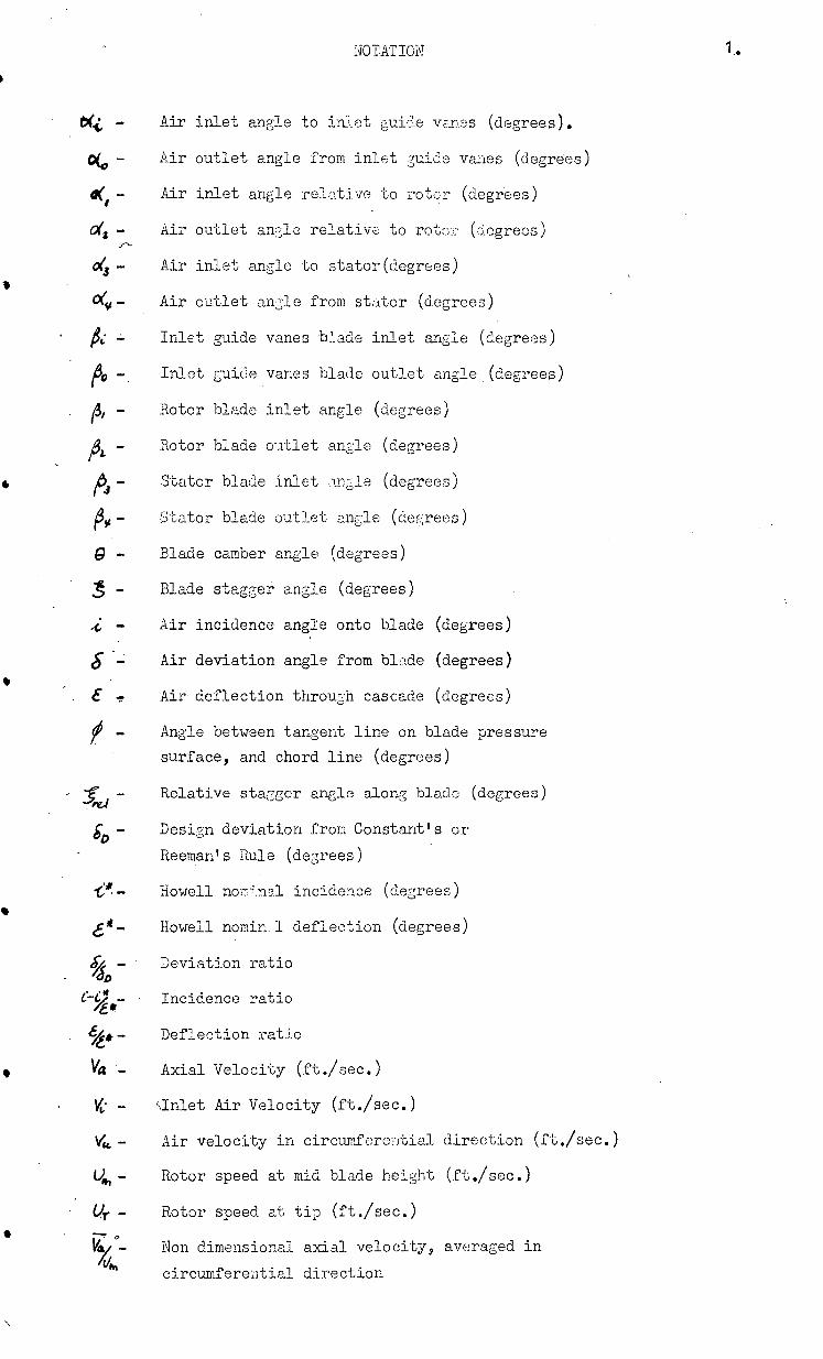
NOTATION

Air inlet angle to inlet gui de vanes (degrees).

Air outlet angle from inlet guide vanes (degrees)

Air inlet angle relative to rotor (degrees)

Air outlet angle relative to rotor (degrees)

Air inlet angle to stator(degrees)

Air outlet angle from stator (degrees)

Inlet guide vanes blade inlet angle (degrees)

Inlet guide vanes blade outlet angle (degrees)

Rotor blade inlet angle (degrees)

Rotor blade outlet angle (degrees)

Stator blade inlet a.11:;1 (degrees)

Stator blade outlet angle (degrees)

Blade camber angle (degrees)

Blade stagger angle (degrees)

Air incidence angle onto blade (degrees)

Air deviation angle from blade (degrees)

Air deflection through cascade (degrees)

Angle between tangent line on blade pressure

surface, and chord line (degrees)

Relative stagger angle along blade (degrees)

Design deviation from Constant's or

Reeman's Rule (degrees)

Howell norfj.nal incidence (degrees)

Howell nomin.2 deflection (degrees)

Deviation ratio

Incidence ratio

Deflection ratio

Axial Velocity (ft./sec.)

sInlet Air Velocity (ft./sec.)

Air velocity in circumferential direction (ft./sec.)

Rotor speed at mid blade height (ft./sec,)

Rotor speed at tip (ft./sec.)

Non dimensional axial velocity, averaged in

circumferential direction

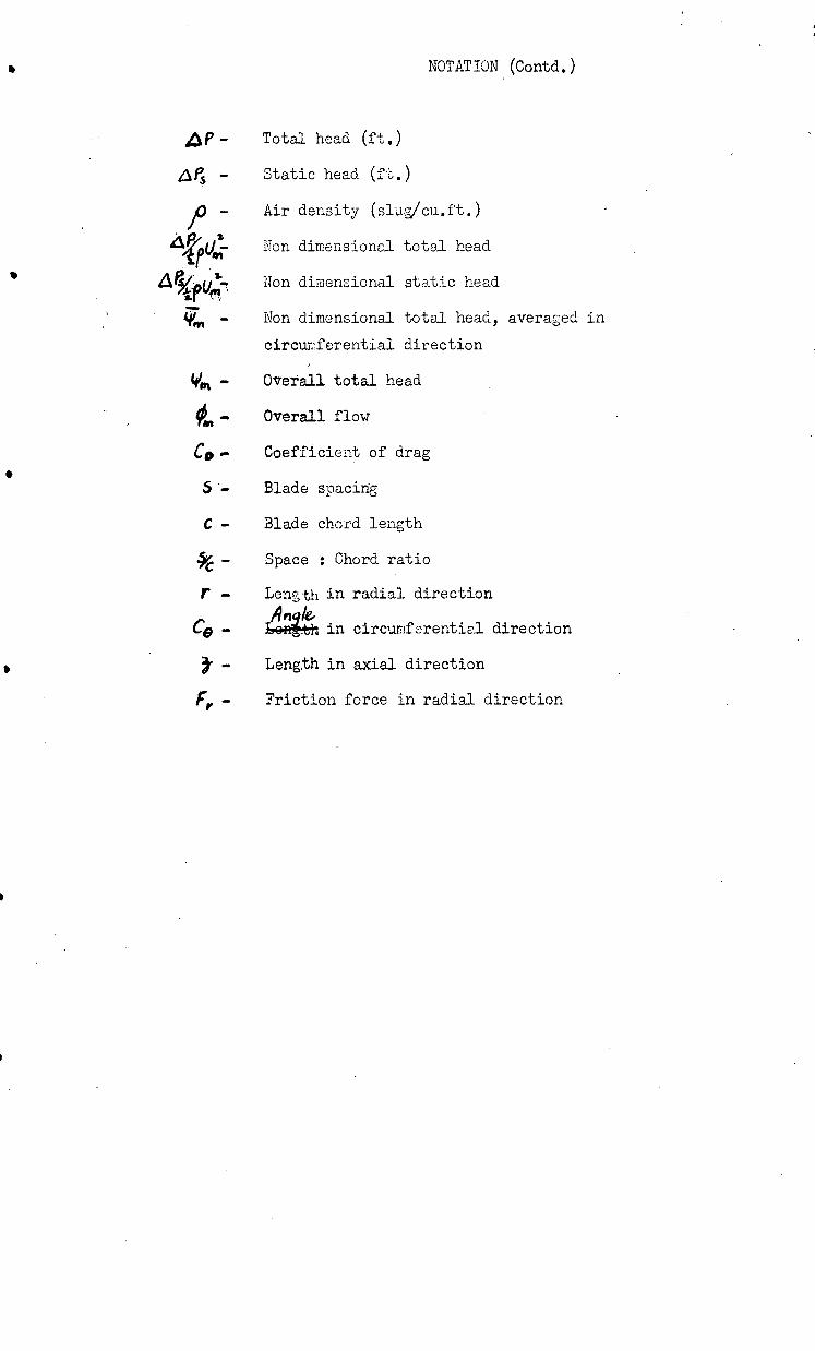
NOTATION (Contd.)

Total head (ft.)

Static head (ft.)

Air density (slug/cu.ft.)

Non dimensional total head

Non dimensional static head

Non dimensional total head, averaged in

circumferential direction

Overall total head

Overall flow

Coefficient of drag

Blade spacing

Blade chord length

Space : Chord ratio

Length in radial direction

Ar1,04 . in circumferential direction

Length in axial direction

Friction force in radial direction

AP -

zles Jo -

Adtptk PYkfur;--

-

3.

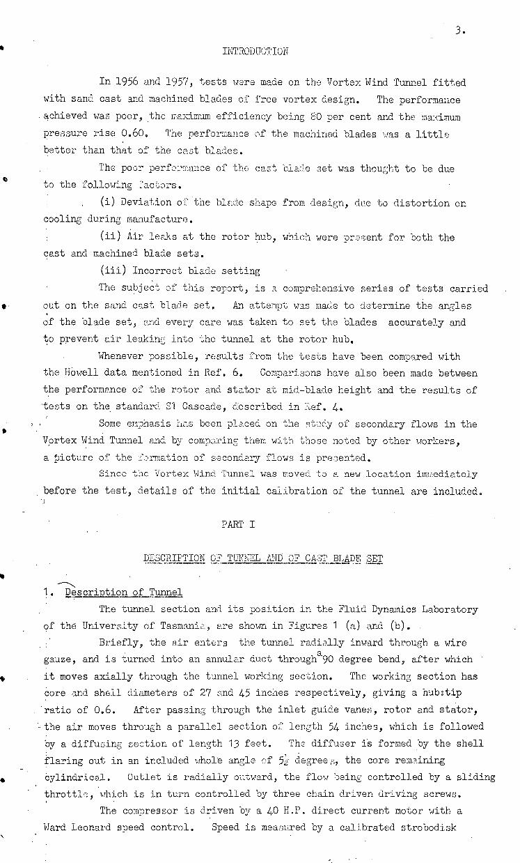
INTRODUCTION

In .1956 and 1957, tests were made on the Vortex Wind Tunnel fitted

with sand cast and machined blades of free vortex design. The performance

_achieved was poor, the maximum efficiency being 80 per cent and the maximum

pressure rise 0.60. The performance of the machined blades was a little

better than that of the cast blades.

The poor performance of the cast blade set was thought to be due

to the following factors.

, (i) Deviation of the blade shape from design, due to distortion on

cooling during manufacture.

(ii)Air leaks at the rotor hub, which were present for both the

cast and machined blade sets.

(iii)Incorrect blade setting

The subject of this report, is a comprehensive series of tests carried

*. out on the sand cast blade set. An attempt was made to determine the angles

. of the blade set, and every care was taken to set the blades accurately and

to prevent air leaking into the tunnel at the rotor hub.

Whenever possible, results from the tests have been compared with

the HOwell data mentioned in Ref. 6. Comparisons have also been made between

the performance of the rotor and stator at mid-blade height and the results of

-tests on the standard Si Cascade, described in 4.

Some emphasis has been placed on the study of secondary flows in the

Vortex Wind Tunnel and by comparing them with those noted by other workers,

a picture of the formation of secondary flows is presented.

Since the Vortex Wind Tunnel was moved to a new location im mediately

before the test, details of the initial calibration of the tunnel are included.

PART I

DESCRIPTION OF TUNNEL AND OF CAST. BLADE SET

1 Description of Tunnel

The tunnel section and its position in the Fluid Dynamics Laboratory

of the University of Tasmania, are shown in Figures 1 (a) and (b).

.Briefly, the air enters the tunnel radially inward through a wire

gauze, and is turned into an annular duct througha90 degree bend, after which

it moves axially through the tunnel working section. The working section has

core and shell diameters of 27 and 45 inches respectively, giving a hub:tip

. 'ratio of 0.6. After passing through the inlet guide vanes, rotor and stator,

the air moves through a parallel section of length 54 inches, which is followed

by a diffusing section of length 13 feet. The diffuser is formed by the shell

flaring out in an included whole angle of 5L degrees, the core remaining

•

Cylindrical. Outlet is radially outward, the flow being controlled by a sliding

throttle, which is in turn controlled by three chain driven driving screws.

The compressor is driven by a 40 H.P. direct current motor with a

Ward Leonard speed control. Speed is measured by a calibrated strobodisk

4 .

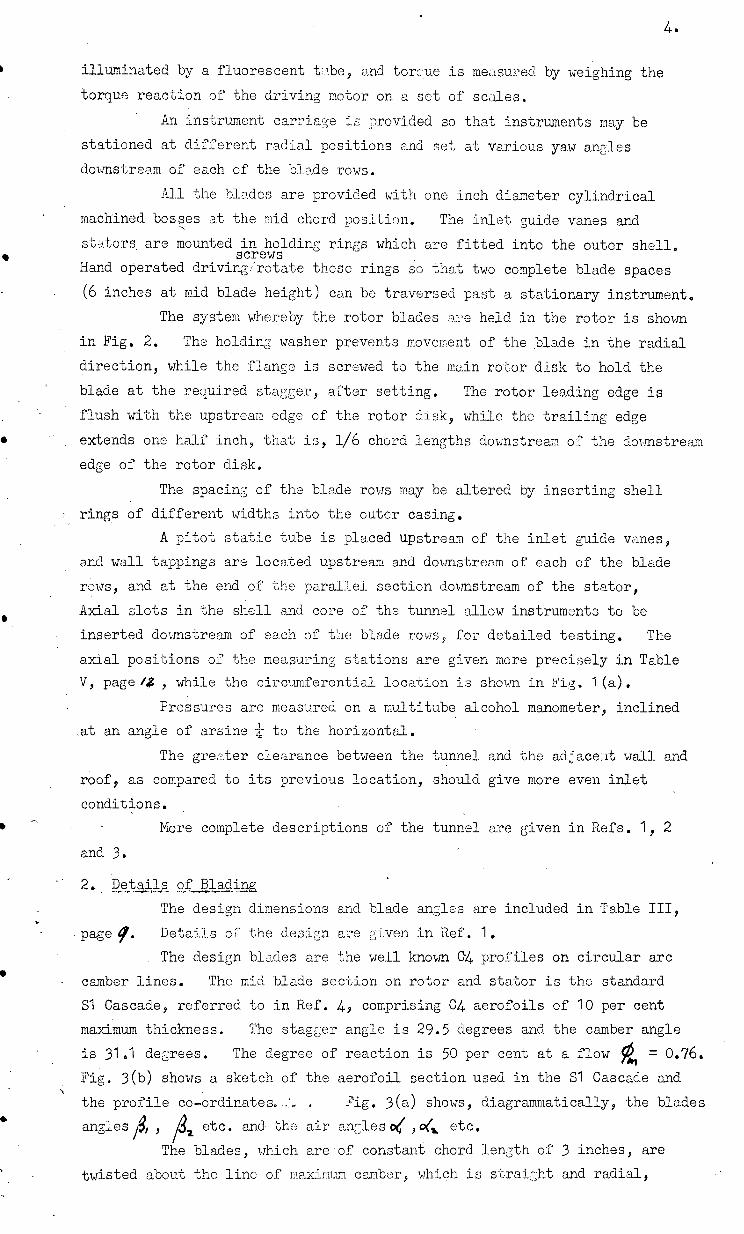
illuminated by a fluorescent tabs, and torc,ue is measured by weighing the

torque reaction of the driving motor on a set of scales.

An instrument carriage is provided so that instruments may be

stationed at different radial positions and set at various yaw angles

downstream of each of the blade rows.

All the blades are provided with one inch diameter cylindrical

machined bosses at the mid chord position. The inlet (7-uide vanes and a stators. are mounted in holding rings which are fitted into the outer shell.

screws Hand operated driving/rotate these rings so that two complete blade spaces

(6 inches at mid blade height) can be traversed past a stationary instrument. The system whereby the rotor blades are held in the rotor is shown

in Fig. 2. The holding washer prevents movement of the blade in the radial

direction, while the flange is screwed to the main rotor disk to hold the

blade at the required stagger, after setting. The rotor leading edge is

flush with the upstream edge of the rotor disk, while the trailing edge

• extends one half inch, that is, 1/6 chord lengths downstream of the downstream

edge of the rotor disk.

The spacing of the blade rows may be altered by inserting shell

rings of different widths into the outer casing.

A pitot static tube is placed upstream of the inlet guide vanes,

and wall tappings are located upstream and downstream of each of the blade

rows, and at the end of the parallel section downstream of the stator,

Axial slots in the shell and core of the tunnel allow instruments to be

inserted downstream of each of the blade rows, for detailed testing. The

axial positions of the measuring stations are given more precisely in Table

V, -page , while the circumferential location is shown in Fig. 1(a).

Pressures are measured on a multitube alcohol manometer, inclined

at an angle of arsine to the horizontnl.

The greater clearance between the tunnel and the adjacent wall and

roof, as compared to its previous location, should give more even inlet

conditions. .

• More complete descriptions of the tunnel are given in Refs. 1, 2

and 3.

2. Details of Blading

The design dimensions and blade angles are included in Table

-page?. Details of the design are given in Ref. 1.

. The design blades are the well known 04 profiles on circular arc

camber lines. The mid blade section on rotor and stator is the standard

Si Cascade, referred to in Ref. 4, comprising C4 aerofoils of 10 per cent maximum thickness. The stagger angle is 29.5 degrees and the camber angle

is 31.1 degrees. The degree of reaction is 50 per cent at a flow A = 0.76.

Fig.' 3(h) shows a sketch of the aerofoil section used in the Si Cascade and

the profile co-ordinates—:. ?ig. 3(a) shows, diagrammatically, the blades • angles/g, etc. and the air angles' ,o4 etc.

The blades, which are of constant chord length of 3 inches, are twisted about the line of maximum camber, which is straight and radial,

5 .

giving nominally free vortex flow at the design point.

The blades, as tested, differed from these design dimensions, as

discussed in the next section.

• To prevent air leaking into the tunnel through clearances of 0.020

and 0,060 inches, upstream and downstream of the rotor between the rotor

disk and the core section, the following precautions were taken to seal off

the core section from atmosphere, The core ends were blocked by masonite

• disks, with rubber sealing rings glued between them and the core, around

:their bearing surfaces, • Molten paraffin wax was poured into the ends of

e the hollow struts which support the core section. The only effect of the

clearances should be some recirculation through them.

3, f Cat, 3et

3.1 Meesurunent Bledes

Sections of the blades were measured by mounting them in a

dividing head on the table of a milling machine and tracing a dial gauge,

fitted with a point contact, over the profile, The reference point

used was where the trailing edge arc appeared to join the pressure

surface of the C4 profile. The blade was traversed underneath the

dial gauge, readings being taken every 0.1 inches near the trailing

and leading edges, and every 0.2 inches elsewhere.

The blade was then rotated 180 degrees and a point similar to

that on the pressure surface was used as reference point on the suction

•

surface, The blade was traversed in a similar manner to that adopted

for the pressure surface,

To enable one surface to be located with respect to the other,

and the leading edge point to be fixed relative to the trailing edge

point, the maximum thickness and chord length were measured with a

micrometer and a set of vernier calipers.

3. 2 Consign of Blade trifles

The blade was drawn five times full size, and the two surfaces

located with respect to each other by assuming that the maximum

thickness occurred at 0.30 of the chord length as given by the co-

ordinates in Fig.

The method of construction used is shown in Fig. 4. Three

. positions, set near the leading edge, near mid chord and near the trailing

edge were chosen, and the mid-thickness points at each, calculated. The

mid-thickness points should have been calculated.for sections perpendicular

to the camber line. • However, since the camber line was then unknown, in

the case of the low cambered and relatively straight inlet guide vanes

and stators, sections in the direction OY were used. For the relatively

high cambered and twisted rotor blades, the directions of the camber

line at each positionwere guessed and the sections were drawn perpen-

dicular to these directions,

A circular arc was drawn through these points by constructing

the perpendicular bisectors CAE and DBF, and extending them until

they intersected at G, the centre of the arc. The circular arc camber

lane was then dray4n through the three mid-thickness points. The same

0

three positions, as nearly as could be estimated, were chosen, to

construct the camber line on all sections.

An arc was drawn tangent to the ',Pressure and suction surfaces near

the trailing edge, to form the trailing edge arc. The point of inter-

section of the substituted camber line and the trailing edge arc, was

assumed to be the trailing edge point, T. The intersection of the

camber line with an arc of radius equal to the measured chord length

of the blade, and having its centre at the trailing edge point T, was

assumed to be the leading edge point L. Line TL was then the chord

line. Angle TGL, which was equal to the camber angle 6 y was

measured. A line was drawn tangent to the -oressure surface, intersecting

TL at J, and its angle with TL, ,Øwas measured. This angle was

required later, for blade setting.

When more than one section of a blade was measured, the angle between

TL and the reference line OX was obtained. OX represented the

table of the milling machine which was kept in the same position relative

to the blade when more than one section was measured. For the different

sections of a blade, this angle gave their relative stagger angles.

The graphical method shown in Fig. 4, was used to measure all the

angles, but in several cases the angles were checked by analytical

geometry, using the same procedure as outlined above. This method,

although eliminating graphical measuring errors was tedious, and in

any case the angle # 1 between the tangent to the pressure surface and

TL could only be determined by constructing part of the blade.

Angles at the mid blade hei ght of six blades each from the inlet

guide vane, rotor and stator sets were constructed in this way. Blade

angles were also measured at the free end and one inch from the boss end

of one blade from each group, and one other blade from each group was

measured at one inch intervals along its length.

At the stations where more than one blade was measured, the mean

of the measured angles was calculated, and the maximum spread of

results was found to be + 0.5 degrees in camber angle and 0.25 degrees

in stagger angle. The majority of the measured angles were in a range

half as wide. Where the blade angles of a section were computed by

both the graphical and analytical methods, the differences were less than

0.3 degrees in camber and 0.2 degrees in stagger. When the corresponding

section on several blades was measured ny the graphical method the mean

value of the blade angles differed from the angles of one of the sections

calculated using the analytical method, by less than 0.1 degrees in both

camber and stagger.

Tests carried out in conjunction with the overall testing of the

compressor suggested that individual differences between the blades were

negligible. Assuming that the blades are similer, the method of

representing them is shown by the comparisons in the above paragraph to

have been accurate and common to sections examined.

In the analysis of results, air angles are referred to the two

4.5

* 29.5

5

29.65

6 , 7 8 9

28.8 27.65 25.7

-1.55 -0.8 -0.55 +0.3 0.6*

31.5 31.0 26.8 21.9 5 18.9 19.0

11.5 4 13.9 15.85 0.75 23.1 25.5

32.9 31.2 32.5 32.0 31.25

1.45 -0.1 -0.5 5 -1.6 5 72 .7

..ens

2 1 3 4

61° 35.5 32.4 31.2 30.9 30.4

1: -3.7 -2.8 -2.6 -1.9 -0.8

47.7 43.5 5 39.4 33.95

-6.2° +0.6 4.7 9.2

32.0 29.9 31.8 31.35

e°

6.25 4.5 4.0 2.2 o

31*/

•

6

7.

dimensional cascade data, presented in Refs. 4 and 6. Difficulty is

encountered in finding the source of differences between the performance

of the blades in the Vortex wind Tunnel, and the performance predicted

from the two dimensional cascade data. One of the reasons for this is

undoubtedly the differences in the flow pattern of a three dimensional

as compared to a two dimensional cascade. However, another source of

difference is that the measured blade angles of the cast aluminium

blade set, do not bear the same relation to the profile as do the blade- • angles referred to in Refs. 4 and 6, and shown in Fig. 3.

The surface roughness of the blades was found by tracing the dial

gauge with the point contact over a small area of a blade surface.

This method is rather crude, but showed the surface . rotOlness to be

the order of 00001 inches to 0.002 inches from the mean, although there

•were some indentations on odd blades which were much larger.

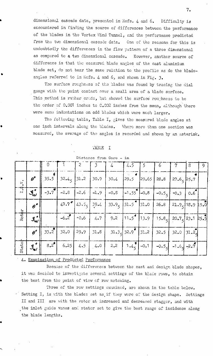
The following table, Table I, gives the measured blade angles at

one inch intervals along the blades. Where more than one section was

measured, the average of the angles is recorded and shown by an asterisk.

TABLE I

Distance from Core - in

• 4. Examination of Predicted Performance

Because of the differences between the cast and design blade shapes,

it was decided to investigate several settings of the blade rows, to obtain

• the best from the point of view of row matching.

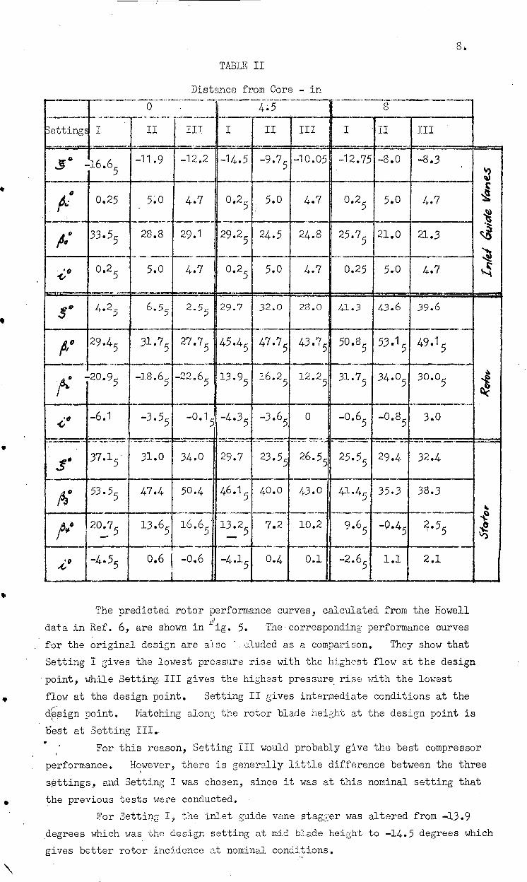
Three of the row settings examined, are shown in the table below.

- Setting I, is with the blades set as,if they were of the design shape. Settings

II and III are with the rotor at increased and decreased stagger, and with

the inlet guide vanes and stator set to give the best range of incidence along

the blade lengths.

Distance from Core - in

0 4.5

II I III I III

TABLE II

S.

- 16.6 5

_11.9 _12.2 -14.5 -9.7 5 -10.05 -12.75 -8.0 -8.3

11s-atom

aPP, Pl`°.7

o # 0.25 5.0 4.7 0.2, 5.0 4.7 0.2 5.0 4.7

A 0 33.55

28.8 29.1 29.25 24.5 24.8 25.7

5 21.0 21.3

1,..,o 0.2 5 5.0 4.7 0.2 5.0 4.7 0.25 5.0 4.7

-- 4.2

5 6.55 2.5, 29.7 32.0 28.0 41.3 43.6 39.6

dCy.Oey

A . 29.45

31.7 27.7 45.4 47.7 43.' 5 50.85 '

53.1 49.1 5

-20.9 5

-18.6 -22.6 13.9 16.2 12.25

1 31.7 5

■

34.0 30.05

..

.C, -6.1 -3.5 -0.1 5

-4.3 5 -3.6 0 -0.6 -0.8 3.0

s ° 37.1

5 31.0 34.0 29.7 23.5 26.5 25.5 29.4 32.4

40

10#.5%

x 53.5 47.4 50.4 46.1 40.0

7.2

43.0 41.4 35.3 38.3

0 20.75 13.6 l6.6 13.2 10.2 9.6 5 -0.4 3.55

.o -4.55 0.6 -0.6 -4.1 0.4 0.1 -2.6 5 1.1 2.1

The predicted rotor performance curves, calculated from the Howell 2

data in Ref. 6, are shown in ig. 5. The correspondingperformance curves

for the original design are also '...cluded as a comparison. They show that

Setting I gives the lowest pressure rise with the highest flow at the design

point, while Setting III gives the highest pressure rise with the lowest

• flow at the design point.. Setting II gives intermediate conditions at the

design point. Matching along the rotor blade height at the design point is

best at Setting III,

For this reason, Setting III would probably give the best compressor

performance. However, there is generally little difference between the three

settings, and Setting I was chosen, since it was at this nominal setting that

• the previous tests were conducted.

For Setting I, the inlet guide vane stagger was altered from -13.9

•degrees which was the design setting at mid blade height to -14.5 degrees which

gives better rotor incidence at nominal conditions.

4easured

0.99 -16.6

g°

-14.5

Rotor Stator

37 38

27" 27"

45" 45" 0,030"(1% span) 0.030"(1% span) 0.033 11 (1.1% span 0.020"(2/3% span)

9 .

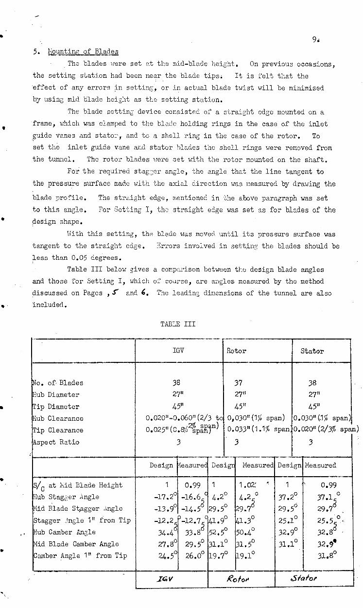
5. Monntim_of_Blades • The blades were set at the mid-blade height, On previous occasions,

the setting station had been near the blade tips: It is felt that the

effect of any errors in setting, or in actual blade twist will be minimised

by using mid blade height as the setting station.

The blade setting device consisted of a straight edge mounted on a •frame, which was clamped to the blade holding rings in the case of the inlet

guide vanes and stator,- and to- a shell ring in the case of the rotor. To

set the inlet guide vane and stator blades the shell rings were removed from

the tunnel. The rotor blades were set with the rotor mounted on the shaft.

For the required stagzer angle, the angle that the line tangent to

the pressure surface made with the axial direction was measured by drawing the

blade profile. The straight edge, mentioned in the above paragraph was set

to this angle. For Setting I, the straight edge was set as for blades of the design shape.

With this setting, the blade was moved until its pressure surface was

tangent to the straight edge. Errors involved in setting the blades should be

less than 0.05 degrees.

Table III below gives a comparison between the design blade angles

and those for Setting I, which of course, are angles measured by the method

discussed on Pages ,Jr and 4, The leading dimensions of the tunnel are also

included.

TABLE III

Design

1

-17.2° -13.9° -12.2 34.46

27.8° 24.5°

IGV

. of Blades

ub . Diameter

ip Diameter

ub Clearance

ip Clearance

spect Ratio

S/ at Mid Blade Height

alb Stagger Angle lid Blade Stagger Angle

Stagger .tngle 1" from Tip

.ub Camber Angle

lid Blade Camber Angle

amber Angle 1" from Tip

3 3

1.02:

29.76

41.3°

50 .4° 31.5° 19.1°

38 27"

45" 0.020"-0.060"(2/3 to

0.025" ( 0 .8% 24aRln) 3

-12.7 °41.9° 33.8 52.5° 29.5° 31.1° 26.0° 19.7°

1

4.2° 29.5°

Design Measured Design Measured

1 0.99

37.2° 37.1 ° 29,5° 29,7g

25.1° 25,5 ° g 32.9° 32.8

31.1° 32.9' 31.8°

Rotoo ,51a/or

10.

PART II

PRELIMINARY TESTS METHOD OF DETAILED-TESTING t INSTMENTATION AND PRESENTATION

1. Preliminary_and Static Tests

1.1 Measurement of No Load Torque

Before the test rotor was installed in the tunnel, a rotor

with blades removed bias mounted on the shaft and torque measurements

were taken for a range of speeds up to 650 r.p.m. Speeds higher than

this could not be tested as small deviations in straightness caused the shaft to vibrate alarmingly.

The no load torque curve, shown in Fig. 6, has been extrap-

olated to 750 r.p.m., at which speed, the error in no load torque may • be as high as + 0.5 ft. lb . At 750 r.p.m. this represents an error of

I per cent for the flows tested. However, as torque is only used as one

check on efficiency, this error is not very critical.

1.2 Investigation of Inlet Conditions

Pitot static tube traverses were made at the top, bottom and

two sides of the tunnel, one chord length (i.e.. three inches) upstream

of the inlet guide vanes leading edge. As instrument carriages are not

provided at these stations, the instrument was held in the hand. The

radial position of the instrument was measured using a steel rule, and it

was held in an axial direction by eye.

Errors in the radial position should be 0.1 inches at most,

and except for the station at the bottom of the tunnel where the experimenter

had to lie on his back, yaw angles of the instrument should be not greater

than 5 degrees. Chapter 4 of Ref. 5 indicates that a yaw angle of 10 degrees in the setting of a pitot static tube, gives readings of total pressure

1 per cent low, and of static pressure 2 per cent low. Thus the diference

between true and measured velocity, due to yawing the instrument, should

be less than 1 per cent.

Tests at 300,500 and 750 r.p.m. were made at various throttle

settings. For one speed and throttle, differences between measured flows

at the four stations, which were obtained by integrating the measured

velocities across the annulus, were less than 3 per cent and generally 1 per cent. Thus, taking into account the possible errors in velocity

due to instrument yaw, the flow seems evenly distributed around the annulus.

The velocity profiles for one station, at one flow condition,

showed variations in the region away from the walls, that is, from 1 to

8 inches from the hub, of about 1 per cent. Hence the velocity may be

assumed to be uniform across the annulus, at the four measuring stations,

away from the wall boundary layers.

There was a tendency for more flow to pass.through the side

stations than through the top or bottom. For the eighteen combinations

of flow and speed examined, the highest measured flow passed through one

of the side stations fifteen times. However, the differences were

so small that it can only be described as a general trend.

1.3 Wall Static Tests

Wall static tapping readings were taken at a range of rotor speeds

and throttle settings, to give an approximate picture of the tunnel

• performance. Readings were also taken from a pitot static tube, placed

one chord length upstream of the inlet guide vanes at the calculated mean

flow height of 5 inches from the hub.

The axial positions of the wall static tappings are listed below —

(i)3 inches upstream of the inlet guide vanes leading edge;

(ii)2 inches downstream of the inlet guide vanes trailing edge;

(iii)2i inches downstream of the rotor trailing edge

(iv)1i. inches downstream of the stator trailing edge. • To draw approximate total pressure versus flow characteristic

curves, the following assumptions were made. ,4xial velocity at the mid

blade height of the rows was assumed to be the same as measured by the

inlet pitot static tube, and the static pressure at mid blade height was

assumed to be the same as measured, by the appropriate wall tapping.

Then assuming that air deviations from the inlet guide vanes were given

by Reemants Rule, and those from the rotor and stator were given by

Constantls Rule, as set out in Ref. 8, approximate absolute velocity and

hence total pressure were calculated.

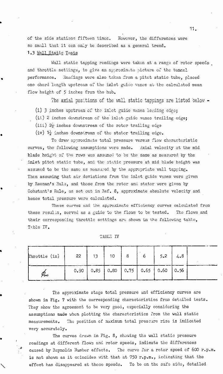
These curves and the approximate efficiency curves calculated from

these results, served as a guide to the flows to be tested. The flows and

their corresponding throttle settings are shown in the following table,

Table IV.

TABLE IV

—

Throttle (in) 22 13 10 8 6 5.2 4.8

4 0.90 0.85 0.80 0.75 0.65 0.60 0.56

The approximate stage total pressure and efficiency curves are

shown in Fig. 7 with the corresponding characteristics from detailed tests.

They show the agreement to be very good, especially considering the

assumptions made when plotting the characteristics from the wall static

measurements. The position of maximum total pressure rise is indicated

very accurately.

The curves drawn in Fig. 8, showing the wall static pressure

readings at different flows and rotor speeds, indicate the differences

caused by Reynolds Number effects. The curve for a rotor speed of 600 r.p.m.

is not shown as it coincides with that at 750 r.p.m., indicating that the

effect has disappeared at those speeds. To be on the safe side, detailed

12,

tests were made at 750 r,p.m. The stator Reynolds Number, based on

vector mean velocity and blade chord length, was 1.5 x 10 5 to 2.2 x•105

for the flow range tested at 750 r.p.m.

2. Instrumentation and Procedure for Detailed Testing

For detailed testing downstream of the blade rows, a-

diameter, Fechheimer cylindrical yaw meter was used. The holes are

0.015 inches diameter and the side holes are spaced approximately + 40

degrees from the total pressure hole.

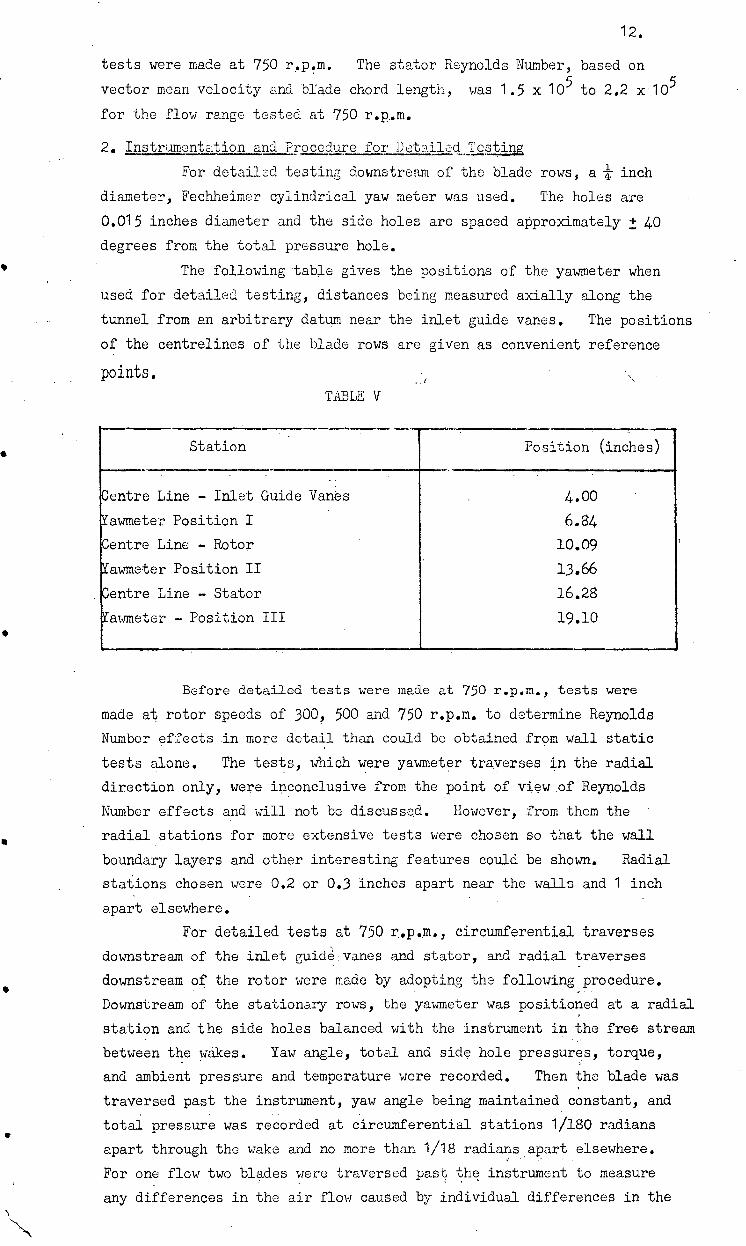
The following table gives the positions of the yawmeter when

used for detailed testing, distances being measured axially along the

tunnel from an arbitrary datum near the inlet guide vanes. The positions

of the centrelines of the blade rowsare given as convenient reference

points.

TABLE V

Station ---

Position (inches)

. .

entre Line - Inlet Guide Vanes 4.00

iawmeter Position I 6.84

entre Line - Rotor 10.09

kawmeter Position II 13.66

entre Line - Stator 16.28

iawmeter - Position III 19,10

Before detailed tests were made at 750 r.p.m., tests were

made at rotor speeds of 300, 500 and 750 r.p.m. to determine Reynolds

Number effects in more detail than could be obtained from wall static

tests alone. The tests, which were yawmeter traverses in the radial

direction only, were inconclusive from the point of view of Reynolds

Number effects and will not be discussed. However, from them the

radial stations for more extensive tests were chosen so that the wall

boundary layers and other interesting features could be shown. Radial

stations chosen were 0.2 or 0.3 inches apart near the walls and 1 inch

apart elsewhere.

For detailed tests at 750 r.p.m., circumferential traverses

downstream of the inlet guide.vanes and stator, and radial traverses

downstream of the rotor were made by adopting the following procedure.

Downstream of the stationary rows, the yawmeter was positioned at a radial

station and the side holes balanced with the instrument in the free stream

between the wakes. Yaw angle, total and side hole pressures, torque,

and ambient pressure and temperature were recorded. Then the blade was

traversed past the instrument, yaw angle being maintained constant, and

total pressure was recorded at circumferential stations 1/180 radians

apart through the wake and no more than 1/18 radians apart elsewhere.

For one flow two blades were traversed past the instrument to measure

any differences in the air flow caused by individual differences in the

13.

blades. • Downstream of the rotor, yaw angle and total and side hole

pressures were recorded at the appropriate radial stations.

3. Calculation of Velocity

To calculate velocities downstream of the stationary rows,

both yaw angle and static pressure were assumed constant in the cir-

cumferential direction. This is in accordance with the test procedure

described in the previous section.

Subsequent tests showed that the yaw angle variation through

the free stream was less than 0.5 degrees, giving a cosine difference of

less than 1 per cent, for the angles measured. An examination of cnicul-ations and measurements taken 1i chord lengths downstream of the low speed, two dimensional cascade, from which Ref. 4 was compiled, showed

that the yaw angle variation across a blade space was, at most, 2 degrees

from the free stream yaw angle. Tests on the inch cylindrical yaw

meter indicated that for the total pressure range eXamined in the Vortex

Wind Tunnel,. a yaw angle of 5-degrees from balance would give an error of

little more thank per cent, providing the flow was two dimensional.

With this proviso, and allOwing that the measuring station is much closer

to the blade row in the Vortex Wind Tunnel, errors made by assuming

yaw angle constant circumferentially should be no more than 1 per cent.

In any case, the behaviour of the cylindrical yawmeter in sheared flow is

unknown, especially since radial flows along it are almost certainly

present, so that any yaw angles measured in a wake would be looked

upon with some suspicion.

Ref. 7 notes that to a first approximation, the static pressure across a wake is constant. This assumption was made for these tests.

Another assumption is necessary to calculate velocity from the

measurements taken. •Velocities at one flow were calculated assuming

side hole pressures to be true static. Then, these velocities were

multiplied by a constant so that the flow obtained by integrating them

across the annulus, checked with the flow measured by the inlet pitot

static tube. This had the effect of adjusting side hole pressure to

true static. The basic assumption made, to calculate velocities in this

manner, was that there were no Reynolds Number effects on the yawmeter.,

Overall, these effects are probably small, since the flows derived

from the calculated velocities checked to within 2 per cent of the corres-

ponding flows, measured by the inlet pitot static tube. The constants

used were 0.839 downstream of the inlet guide vanes and stator, and 0.866

downstream of the rotor.

Check calibration tests in a small calibration tunnel showed

that there was a 10 per cent variation in the ratio of velocity, calculated

from the difference between total and side hole pressures of the yawmeter,

and true velocity. The Reynolds Number range was 3.5 x 103 to 11 x 103 ,

based on instrument diameter and free stream velocity. The results of

these tests were used to try and determine velocities in the Vortex Wind

1 4. Tunnel, but the attempt was unsuccessful, probably due to higher

turbulence levels,

By using one yawmeter constant across the tunnel annulus,

velocity is overestimated near the walls and underestimated elsewhere.

However, since the areas affected by the walls are small, the underestim-

ation near mid blade should be less than 1 per cent. The error may be

larger in the wall regions.

4. Discussion of Errors Involved in Measurements

4. 1 Torgaq

As mentioned in page/0 , the error in no load torque may

be as large as + 0.5 per cent. Because of the vibration of the

needle when the tunnel wasoperating, the torque reading could not

be made to better than t 0.5 ft. lb ., introducing another error'

of per cent. Hence, assuming that the scales read the correct

load, the error may be as high as ± 1 per cent. An attempt to

calibrate the scales themselves proved unsuccessful. As mentioned

before however, torque measurements were only used for calculating

efficiency, which could be checked by another method, so that errors

in torque were not really critical.

4.2 Rotor Speed

The measured rotor speed which was obtained by reading the

calibrated strobodisk illuminated by a fluorescent tube, was dependent

on the frequency of the domestic power supply. It is possible to

detect a difference of 1 r.p.m., by the apparent movement of the

strobodisk and frequent checks and adjustments were constantly made

to the speed.

The variation of the frequency of the power sup2ay was

investigated using a frequency counter. It was found to be less

than 1/6 per cent, apart from odd fluctuations of up to per cent

which lasted for only a few seconds. Hence any errors made by

dividing pressures and velocities by (6, and respectively, to

make them non dimensional, should be small.

4.3 XAE_IBEI2

From experience in testing the Vortex Wind Tunnel with the

cylindrical yaw meter, yaw angles cannot be consistently repeated to

better than 0.2 degrees. - This angle is very small as far as its

effect on computations are concerned, as the cosine difference in the

range of angles tested is only per cent, and the tangent difference,

1 per cent.

4.4 Measurinc, Station

The measuring station adopted, as shown in Fig. 1(a) was

on the side of the tunnel furthest away from the nearest wall of

the building; that is, the most favourable from the point of view

of inlet conditions.

•5.

It was noted on page /42 that there was a tendency for more

flow to pass through the side stations, than through the top or bottom.

At the positions A and B indicated in Fig.1(a) the inlet clears

the base frame by only 6 inches. Because of their inaccessibility,

inlet conditions at these two stations were not measured, but it is

to be expected that the flow through them is lower than elsewhere.

Hence, overall flow, total pressure rise and efficiency may

be overestimated to some extent, but this of course, has no effect

on the performance of individual blades.

5. Presentetion

The averages with respect to length in the circumferential

direction at one radial station, of total pressure and axial velocity _- across a blade space are denoted by Kt, and 161k In the case of the

inlet guide vanes and stator, these wlues were obtained by direct

comoutation. For the rotor, the yawmeter was assumed to have measured

this average of total pressure, and when continuity had been satisfied,

to have measured the same average of axial velocity.

The symbols Vt, and tare used for the rotor and stage total pressure rise and overall air flow. pt. is measured by the

inlet pitot static tube upstream of the inlet guide vanes andtis calculated _- • from the computed values oft, and is an area average of cover the

annulus. t was also Calculated from a flow average over the annulus,

which gave values 2 per cent higher than from an area average. Since

this gave peak rotor efficiencies of 97 or 98 per cent, which was much

higher than expected, the area average method was preferred.

Throughout the test, when velocities and totA and static

'pressures are mentioned, they refer to the appropriate non dimensional

values, unless otherwise indicated.

•

•

16.

PART III

DETAILED SURVEY. OF RESULTS

1. Stau Performance

The stage pressure rise and efficiency curves are shown

in Fig. 9, with the appropriate total pressure rise curve plotted from the data in Ref. 6.

1.1 Discussion of Methods of Predictin7 compressorT„erformance

1.1.1 Methqd Due to A.R. Howella_Given in Ref. 6.

The data presented in Ref. 6, is obtained from tests

on two dimensional cascades. The overall performance of the compressor was predicted by calculating the Howell performance

at the rotor and stator mid blade height sections. Since

the downstream air angle of all rows at the design flow of

= 0.76 was fixed with the setting of the blades, nominal

air alvaes for each row were automatically determined, and

the rotor and stage characteristics were then drawn from the

two dimensional cascade data.

In previous tests, the agreement between the measured

and predicted overn11 characteristics has been very good. - This

is in line with similar comparisons shown in Ref. 13.

In Sections 2.3 and 3.3 of Part III, the Howell data is also used as a basis for examining the performance' of

individual blade sections. Its primary purpose is a basis

for preliminary design, and although it is apparently unsuited

to detailed analysis of three dimensional compressor cascades,

its predictions of air outlet angle and total pressure rise are,

in most cases, quite accurate.

The main points of difference between two dimensional

cascade data, and the performance of sections in the Vortex

Wind Tunnel, are listed below:

(i)The design curves presented in Ref. 6 are an average of results from two dimensional cascade tests of several C series

aerofoils. Fig. 29 shows that the difference between the

measured and predicted deflections through the two dimensional

Si Cascade is up to 2 degrees. Howell, in Ref. 13 notes that

a difference of 1 degree in deflection alone, makes a difference

of 6' per cent in total pressure rise.

(ii)Flow through the compressor is assumed to be cylindrical.

The discussion of Fig. 11 on pagesiz and33 shows that it is

not, as the measured flow movement is as large as 5 per cent of the blade height.

(iii)Conditions downstream of a blade row are not taken into

account. An annlysis on page 22 of the performance of the

Vortex Wind Tunnel rotor shows that a complete stall of the

rotor was postponed by a tip stall of the stator. This effect

17 could not have been predicted from the Howell data.

(iv)In Section 8, Part III , differences between the

boundary layer migration effects in two and three dimensional

cascades are discussed. In the Howell design. system, these

effects are lumped together into an extra drag term.

Comments on pa ges 24 and U indicate that they nlso play

some -part in affecting distributions of pressure and yaw

angle.

(v)No account is taken of the fluctuating flow, consisting of alternate wakes and free stream regions, which is presented to the rotor and stator from the upstream blade row. From

material given in Ref. 7 concerning work on oscillating

cylinders, it seems unlikely that this flow pattern results

in momentary separation of the flow from the blade and its

subsequent reattachment. It seems more likely that, because

of the short time that low speed air in a wake is incident

onto the blade, the final result is a thickening of the boundary

layer on the blade, resulting in slightly higher air deviations

' from it.

1.1.2 Method Due to A.D.S. Carter

The Carter method of predicting the performance of

cascades of aerofoils is given in Ref. 15. Curves of non

dimensional incidence against non dimensional deflection, plotted

in Figs. 19 and 23 include stalling incidences plotted from this data.

The optimum incidence, which gives the lift: drag ratio

a maximum, is assumed to occur at the leading edge of each blade.

The cascade is replaced by a row of vortices, because of the shape

of the -pressure distributions on the suction and pressure surfaces

of each blade. Both the vortex row and the action of a blade (or

vortex) on its neighbours, which depends on the blade spacing,

involve adjustments to the direction of the upstream air to give

optimum incidence.

Using two dimensional cascade data, derived from Cl

aerofoils, but which, he claims, should also apply to C2 and

C4 profiles, several useful refinements are produced. For

instance, stalling incidence may be obt ained. Also, critical

Reynolds Number, corrections for variation in stagger angle of a

cascade, and the effects of the position of maximum camberand

maximum thickness are discussed in :eeneral terms. These

provide useful additional knowledge for compressor design, and

although performance curves from this data were not plotted,

stalling incidence, as shown in Figs. 19 and 23, is predicted

quite closely.

1.2 Stage Pressure Rise

The stage pressure rise curve, shown . inFig. 9, gives

pressures lower, except at the high flows, than those predicted from the

18.

Howell data. The reason for this is not apparent without a detailed

examination of the rotor and possibly the stator, performance. In

the region of the design flow, 4t = 0.76, the gradient of the design

curve is higher by about 50 per cent. Referring to Fig. 5., the

difference between the Howell and measured characteristics, is some-

what similar to the difference between the mid blade characteristics

of Setting I and Setting III. That is, the difference is similar

to that produced by altering tlYJ rotor starer by a few degrees. 1.3 Stagc Efficiency

The stage efficiency shown in Fig. 9, is flat and

indicates that the efficiency is high over a wide range of flows.

Since the rotor and stage efficiencies were calculated from the

overall pressure rise and flow and the measured torque, they may

be more than 1 per cent in error. However, Table VI, on page 27,

which compares stage efficiencies calculated by two methods, suggests

that the curve in Fig. 9 gives a . fair picture of the efficiency

characteristics, differences being not larger, in general, than

1 per cent.

2. Rotor Performance

2.1 Presentation and _Calculations The rotor predicted and measured total pressure rise

characteristics and the efficiency curve, are shown in Fig. 9. Radial distributions of deviations from the inlet

guide vanes at various flows, are shown in Fig. 10. They are

plotted a4C where 45; is the predicted deviation calculated from oft' Reemanrs Rule, as in Ref. 8.

Radial movement of flow is shown in Fig. 11. Only

those at the four smallest throttles tested are given, as for the

other three flows, the movement was too small to be plotted. The

movement was calculated by integrating the measured values of ;sr, across the annulus at each measuring station, and plotting the

corresponding integrated flow positions.

Predicted and measured curves of air outlet angle 06 ,

and total pressure rise at stations 1 inch apart across the annulus,

are drawn in Figs. 12 to 18. The predicted values were calculated

from the Howell data using values of axiR1 velocity and yaw angle

measured downstream of the inlet guide vans, at the appropriate

stations. The axial velocity Ili; was used as the rotor was assumed rum

to "seen this average of the wake and free stream velocities.

Comparisons between predicted and measured vnlues of0<y were preferred

to comparisons of Va , as calculatingoyrom measurements downstream

of the rotor involves-two assumptions, both of doubtful validity,

which are discussed below.

(i) The yawmeter measures a certain average of the wake and free

stream velocities downstream of the rotor, What average this

is, is unknown, since it depends on the damping characteristics

19.

of the yawmoter, connecting tubes and manometer. The measuring

setup is heavily overdamped which suggests that the average of

total pressure which is measured by the yawmeter is closer to free

stream total pressure and hence is hi gher than a simple average

over a blade space, similar to those calculated downstream of the

inlet guide vanes and stator. Because of the larger wakes near

the walls 9 total head y aff:. hence velocity in the region of the walls is hi[:,:her than true velocity, bringing about a decrease in

calculated velocity away from the walls, as compared to true

velocity when continuity is Satisfied. This accentuates errors

caused by Reynolds Number effects, as discussed on page Af .

(ii) The wake downstream of the rotor has a certain momentum or

displacement thickness. In a later section, Section 5, use is

made of the similarity in blade shape between the mid blade sections

on the rotor and stator to assume a momentum thickness for the rotor

wake. However, similar assumptions about other blade sections

are considered to be unwarranted.

In discussing values of eitherall or P(3 it should be

kept in mind that yaw angles measured by the yawmeter downstream

of the rotor, are some average of the yaw angles of the wakes and

free stream regions, Without making assumption (ii) above, and

having some knowledc:e of the damping characteristics of the system

which measured side hole pressures, it is impossible to estimate

the variation in or what average of it, the yawmeter measures.

This instrument error is only 2 or 3 degrees at most, and is

almost certainly much less.

Curves of deflection ratio,,0aOttea:aZainst .inoidence . .„

ratio c* for various stations along the rotor, and. at various flows

are shown in Fig. 19. The ratios are the same as used in Ref.

6. Deflection was calculated from the measured values of $6 and vsm,

(113 downstream of the rotor, by assuming no wakes, but since the

curves are used for comparison purposes only this does not matter.

The r adial distributions of

plotted in Fig. 20

are presented in a similar manner to those for the inlet guide

vanes shown in Fig, 10. Values ofi. were calculated by assuming

no wakes from the rotor so are also used for comprison purposes

only. was computed using Constant's Rule, in Ref. 8.

Radial distributions of total pressure as measured

by the yawmeter downstream of the rotor, and of axial velocity

as calculated to satisfy continuity, are given in Figs. 21 and 22.

When examining the total pressure rise and deflection

through a section of the rotor, the flow was assumed axial.

Although this is not so, as demonstrated in Fig. 11, the discussion

on page fl , dealing with flow through the stator, shows that with

tho present knowledge of flow in compressors, no other assumption

has any greater validity.

20.

. 2.2 The petectiqn_pf_qtall

For purposes of design, an empirical stall point involving

the achievement of some chosen drag, signifies. that the blade has

stalled. .=./1 exmole of this is given in Ref. 6, where the ,

stall point is taken as occurrin when losses reach twice their

minimum value.

When detailed treverses, such as those downstream of the

stator are available, the fixing of an. empirical stall point is relatively simple. Downstream of the rotor, detailed measurements

cannot be made, and other means of detection must be used.

Curves drawn in Ref. 6, show that at the arbitrary stall

point, the lift and hence the deflection curves, have flattened off.

Thus, when overall flow is decreased, a corresponding decrease in

total pressure or air deflection at a station, is an indication that

the empirical stall point has been reached, or is beim'. approached.

The blade may be said to be in a "stalling condition." Whenever the

term stall is used in this text, it means that the blade seation is in

this "stalling condition".

2.3 Discussion of Results

2.3.1. Rotor Overall Performance

The comoarison between the predicted and measured total

pressure rise characteristics, is similar to that between the

predicted and measured stage characteristics, especially with

regard to the higher gradient of the predicted curve. However,

agreement is better in the region of the design flow of le ' = 0.76

and generally, Fig. 9 suggests that stator losses are larger than

predicted. Also, as the flow is decreased from 1/14, = 0.60 to

0.56, rotor overall total pressure rise increases, while that for

the stage decreases, indicating high stator losses at = 0.56.

Maximum measured rotor. efficiency is about 96 per cent, which,

as discussed on page/4 , may be in error by 1 per cent or more,

because of incorrect torcue measurements and overestimation of 27

flow. However, as mentioned on page /8 the table on page suggests

that the errors are no larger than 1 per cent.

2.3.2 Inlet Guide Vane Deviations

The curves of y plotted for the inlet guide vanes in

Fig. 10, show deviations are higher, and hence deflections

lower, than expected, by at least 2 degrees.

When predicting the inlet guide vane deviations from other

compressors installed in the Vortex Wind Tunnel, Reemants Rule

has agreed with measurements to better than ir degree over the

greater part of the annulus. On page 7 , reference is made to

possible sources of difference between predicted and measured

air angles in this test. One of them was that the measured

blade anzles, from which the predictionswere made, do not bear

21.

the same relation to the blade profile, as do the angles in

Fig. 3. Taking into account the reliability of Reeman's Rule

in previous tests, measured deflections at a given incidence,

which are 2 degrees lower than those predicted from the Howell

data, will be attributed to this cause. This 2 degrees

difference will be called the 4:blade distortion effect."

The effect of theincreased inlet guide vane deviations, is

to increase the incidence onto, and hence the pressure rise

through the rotor, for a given flow. Thus the overall pressure. rise characteristic will be raised.

2.3.3. ;qotor.. Outle.t_Air Angles

Curves of measured and predicted values of q(, (Figs. 12 to 3

18), show measured angles generally lower than those predicted,

suggesting increased deviations from the blade,

An error was made in instrument traverses downstream of the

inlet guide vanes at AI = 0.56, and predictions at this flow

are not included. It was considered unnecessary to rerun the

tunnel to gain results of inlet guide vane performance, at a

flow approaching surge.

The effect of the yawmeter measuring an average of the wake

and free stream yaw angles, as mentioned on pagel, should be to

increase the measured . angle, since the yaw angle of the wakes must

be higher than of the free stream regions.

Generally, considering the possible 2 degrees difference due

to the "blade distortion effect" the a greement at stations 2 to 5

inches from the hub, where the difference is 2 degrees or less,

is remarkably good. At .stations 1, 6, 7 and 8 inches from the

hub, the difference is much larger being up to 5 degrees. With

decreasing flow the difference between corresponding predicted and

measured curves increases, especially for those stations . where

the agreement was best. This comparison is similar to that

between the Howell and measured curves for the Si Cascade, shown

in Fig. 29. One interesting feature is the large increase in

air outlet angle as flow is decreased from 041 = 0.60 to 0.56, indicating a decrease in deviation, from that expected.

The curves ofie from the rotor, drawn in Fig. 20 give the

effects mentioned above, especially the increased deviations in

the region of the tip. =owing for the "blade distortion effect",

it seems probable that the poor tip performance is a result of

boundary layer migration to that region, which is discussed in a

later section on pages.* and 37. The deviation curves for = 0.60 and 0.56, afford an

interesting comrarison, as the deviations at = 0.56 are lower .61

from the hub to 2 inches from the tip, and higher from there to

the tip. This shows clearly the effect noted with the air outlet

angles plotted in Figs. 12 to 18. Referring to Fig. 19, where

the deflection ratio fnlls off after / = 0.65 and picks up

22.

after = 0.60 for all stations except at 1 inch from the

tip, it is apparent that at # = 0.65 the rotor is on the

point of stall, and has actually stalled at p6= 0.60. However, ac, as the flow is further decreased the stall becomes more severe

inthe tip region, and the remainder of the flow accelerates

through that part of the annulus nearer the hub. The rotor

tip stall and subsequent flow acceleration seems to be a result

of a stator tip stall at AL = 0.60, which becomes very severe

at A 0.56. The stator tip stall is discussed on page. A.

The result of the flow acceleration is an increase in deflection

and also an increase inpressure rise. Apparently the acceleration

was not large enough to prevent the high deflections giving

correspondingly high pressure rises.

The large radial movements of the flow at the lower

throttle settings, are illustrated in Fig. 11. The effect of

acceleration through the mid blade and hub regions at = 0.56, is shown by the axial path taken by the flow, compared to the

radially outward movement at hir2:her throttle settings.

2.3.4. Rotor Total Pressure Rise

The comparisons between measured and predicted total

pressure rise along the rotor, are similar to those for the

outlet air angles. The agreement is best from 2 to 5 inches

from the hub, and worst in the tip region. The rotor recovery •

at pf, = 0.56, mentioned on pagesu and 22, is shown in Figs. 12 to 15, although Fig.18(h)suggests that the tip is completely

stalled at that flow, The non agreement between the predicted

and measured overall rotor total pressure rise characteristics

shown in Fig. 9, is due to the low pressure rise obtained from

the rotor tip. Ae the characteristics drawn in Fig. 5,show;

at the low flows the tip repsion makes the greater contribution

to the work output, so that the poor performance of the tip

has a marked influence on the overall total head rise.

Which of the possible reasons for differences between

measured and predicted -1-irformance, as discussed on page7

has caused this, is difficult to determine. On pages 36 and 3f there is some discussion on the possibility of low energy air

migrating in the rotor boundary layers to the tip region, piling

up there, and so interfering with the flow in that region.

However, the effect is so extensive, since rotor performance

is much lower than expected for 3 inches from the tip, that the

explanation probably lies in a combination of boundary layer

migration and the hblade distortion effect."

The velocity distributions downstream of the rotor, shown

in Fig. 22, indicate that the axial velocity across the annulus

was, in general uniform. The increasing thickness of the hub

and tip "boundary layers" is a phenomenon noted in previous

tests described in Ref. 3, and is caused by the spreading of the

23.

secondary flows and a general thickening of the boundary layers

themselves, with decreasing flow.

2.4 Conclusions

The Howell predictions seem fairly good away from the wall

regions. However, it is possible that the two effects noted on

page 7, neutralise themselves in the mid blade height region to give

this agreement.

If the difference due to the "blade distortion effect" is

taken as 2 degrees, then the agreement is very good ) considering the sources of error discussed on pages 45 and /7.

The differences between the predicted and measured overall

characteristics can be explained by the poor performance of the rotor '

tip, which is attributed to the influence of boundary layer migration

to the tip and the 2 degrees "blade distortion effect."

The effect of downstream conditions on the performance of a

row, is demonstrated by the pick up of the rotor at 4.= 0.56 after it had apparently stalled at gL= 0.60. This is caused by a stall at

the stator tip at IL = 0.60 and 0.56 which causes a flow acceleration

through the rotor away from the tip region.

The rotor efficiency is high over the whole operating

range and, in spite of some reservations about the accuracy of the

results, seems to conform to other measurements.

The Carter stalling incidence, plotted in Fig. 19 is quite

close to the incidence at which the deflection decreases from its

peak, so that it gives a fair estimate of the "region of stall."

3. Stator Performance

3.1 Presentation and Calculations

Comparisons between predicted and measured air outlet

angles from the stator are shown in Figs. 12 to 18. The predicted

angles were calculated from the air angles measured by the yawmeter

downstream of the rotor, using the Howell data. The stator was

assumed to "see" the same average of yaw angle as measured by the

yawmeter, so that these predictions are subject to the same errors

of yaw angle as have been discussed on page 1.

Curves of incidence ratiodl.tagainst deflection ratio4/0

are plotted in Fig. 23, the values being obtained from yaw angle

measurements downstream of the rotor and the stator. The curves

are similar to those in Fig. 19, except that air outlet angle from

the stator was measured directly, and no assumptions were made about

the wakes, as was the case with Fig. 19.

Radial distributions of axial velocity, total pressure C. •

and deviations & are shown in Figs. 24 1 25 and 26. 1- .4b

Radial distributions of loss downstream of the stator at

various flows, and loss at each station downstream of the stator

for varying flew, are shown in Figs. 27 and 28. The losses were

taken as the differenpe between fl!:,0e stream total presswe and the

24.

average total pressure across a blade space. P_ method of measuring

losses dae to A. Betz is discussed in Ref. 7, and the first term

of the Betz expression is the difference between the average and free

stream total pressures. The second term is a correction, the magnitude

of which depends on the variation in static pressure through the wake.

Thus the correction term becomes smaller the further the measuring

station is moved downstream of the blade row. On pages Viand/ a

comparison between the losses at the stator mid blade height and the

losses through the Si Cascade is discussed, the comparison being shown

in Fig. 29. Adding the correction term to the stator losses made a difference of less than 10 oer cent, that is, less than 1 per cent in

measured total head, which is considered the limit of accuracy of the

yawmeter, and therefore too small to be significant.

3.2 Discussion of Other Work

Both the Howell and Carter methods of predicting cascade

perfermance have been discussed on pages /6 and In Ref. 10,

Carter refers to drag traverses downstream of a two dimensional cascade.

The curves showing drag distributions rise to a peak near the wall and

then fall off to almost zero at the wall itself. No mention is made

of the method of measurement, which is a drawback when comparing these

curves with the results in Figs. 27 and 28. Drag distributions

similar to those for the two dimensional cascade are given for a radial

cascade of untwisted blades.

The effect of secondary flows on the air outlet angle from a

cascade is also discussed in Ref. 10. Because of t he various sources

of error discussed on page 1 , which are present when measuring air

outlet angle from the rotor, discussion'of.the influence of secondary

flows on air angle will be confined to the stator.

3.3 Discussion of Results

3.3.1 Stator Outlet Air Angie

The differences between predicted and measured air outlet

angle from the stator, shown in Figs, 12 to 18, are with one

exception, 2 degrees or less. At the station 8 inches from the

hub the difference is as large as 5 degrees. Thus the agreement

is generally very good since, as was discussed on page2/, 2

degrees difference might be expected from the "blade distortion'

effect".

The poor agreement at 8 inches from the hub is possibly

due to a vortex from the rotor tip. Work in Ref. 11, which is

discussed in detail in Section 8.3.3 shows flow separation on a

cascade caused by a vortex from another cascade upstream. Although

these corner vortices are present both at the hub and the tip, the

tip vortice from the rotor has a higher circumferential component

of velocity than the one at the hub and should therefore, because

of its higher total energy, exist for a loner time and hence

distance, down the tunnel. This explains why the agreement is

poorer at the stator tip than at the stator hub.

25.

At stations 1 and 6 inches from the hub, there is a sharp

increase in outlet angle, that is, in deviation, as the flow •

is decreased from= 0.60 to 0.56. Exactly the opposite

effect occurs at the station 3 inches from the hub. The reason

for this may be local stalling alone the blade as the flow is

decreased. Because of the irregular surface of the blades it is

'possible that one section may stall at a higher flow than an

adjacent section, producing local accelerations which result:

in higher deflections. This is a similar effect to that for the

rotor discussed on page 22. . Although Fig. 23 suggests that the

stator is working at a lower incidence than the stalling incidence

predicted from the Carter data, yet the difference between it and

the maximum positive stator incidence is only about 2 degrees.

This 2 degrees can easily be accounted for by errors in yaw angle

measurements downstream of the rotor and in the "blade distortion

effect."

The curves in Figs. 12 to 18 indicate that the agreement

is generally best at = 0.65 and 0.75 and becomes worse with

increasing flow although the difference is still within 2 degrees.

The curves in Figs. 19 and 23 suggest that the stator is

working in a lower incidence rane than the rotor, since it is

most likely that differences between predicted and measured air

angles due to the 'blade distortion affect" are approximately

the same on rotor and stator. Thus at the high flows, = 0.90

0.85, and especially at stations near the tip, the stator is

working at high negative incidence. This may account, in part,

for the comparatively poorer agreement between predicted and

measured air outlet angles in the high flow range.

• The curve of incidence ratio against deflection ratio

at 8 inches from the hub, in Fig,23, suggests a stall at the

lowest flow. This is supported by Fig. 28 which shows a sharp

increase in losses at the stations 7 and 8 inches from the hub,

at Ff = 0.56. The effect of this stator tip stall on rotor

performance has already been discussed on page 22. The other

curves in Fig. 23 show no interesting features except that there

is some recovery in deflection at of = 0.56, which is probably

a result of flow acceleration similar to that through the rotor.

The diagrams in Fig. 11 sug gest some radial flow movement towards

the mid blade height region at that flow.

The radial distributions ofSA I plotted in Fig. 26, show '40,o

the same form as the curves of outlet angle plotted by Carter

in Ref. 10, as they have similar peaks near the walls and a

depression near the centre of the passage. The effect of the

stn11 at 7 and 8 inches from the hub at gt.= 0.56, is to decrease

the deviations in the tip region below those at Al , = 0.60.

However, any attempt to discuss these phenomena in detail is

26.

rendered suspect by the probable errors in measured yaw angles

near the wall, The lower deviations in the hub region at

= 0.56 compared to 0= 0,60, ate most likely to be a result - of the flow acceleration mentioned on page and shown in Fig. 11.

3,3,2 pi:stributionspf Flow ant_TptAl_Pressure_Downstream Statot

The irregularities in these curves, shown in Figs. 24 and 25,

are largely attributable to irregularities in the blades themselves,

although the pronounced lip in the curves near the hub is a

manifestation of a vortex or pair of vortices in that region. These

are further discussed on pages 313 and 3/. Generally, both sets

of curves follow the corresponding rotor curves fairly closely.

However, the diagrams of flow movement in Fig, 11, indicate that

boundary layer growth at the stator hub ; causes a radially outward

movement of the flow through the stator.

3.3.3 Losses_Tbrogh the Stator

The radial distributions of loss in Fig. 27, show features

different from those in Ref, 10, Generally, the p3aks in Fig.

27 are at the station nearest the wall, although the curves at

= 0.65, 0.60 and 0,56 suggest some decrease in loss at that

station. The large loss peak near the hub, compared with that

at the tip, is attributed to the radial transport of low energy

air to the hub. This is further dealt with on page 42

At the three highest flows, there is a subsiduary loss

peak near the hub, similar to a loss distribution curve in Ref. 10,

which is plotted dovnstream of a cascade with an If shaped

velocity distribution incident onto it,, Although the peaks are

small and may be the result of measurement errors ; it is most

likely that they are caused by twin vortices in the hub region.

These are further explained on page 38,

The stator losses were used in a check on stage efficiency.

The rotor and stage efficiencies, shown in Fig. 9, were calculated

from the work output of the Compressor, which is the product of

total pressure rise and flow, and the work input from the measured

toque0 In gas turbine practice, the work output of the

machine is obtained from the stage temperature rise. However at

the low rotor speeds, encountered in the Vortex Wind Tunnel,

the temperature rise is too small to measire. The rotor

efficiency calculated from the measured torque and rotor pressure

rise and flow ; was multiplied by the stator efficiency obtained

from the stator losses to give Stage Efficiency I in Table VI

below. Stage Efficiency II wa9 obtained from the stage pressure

• rise and flow.

27.

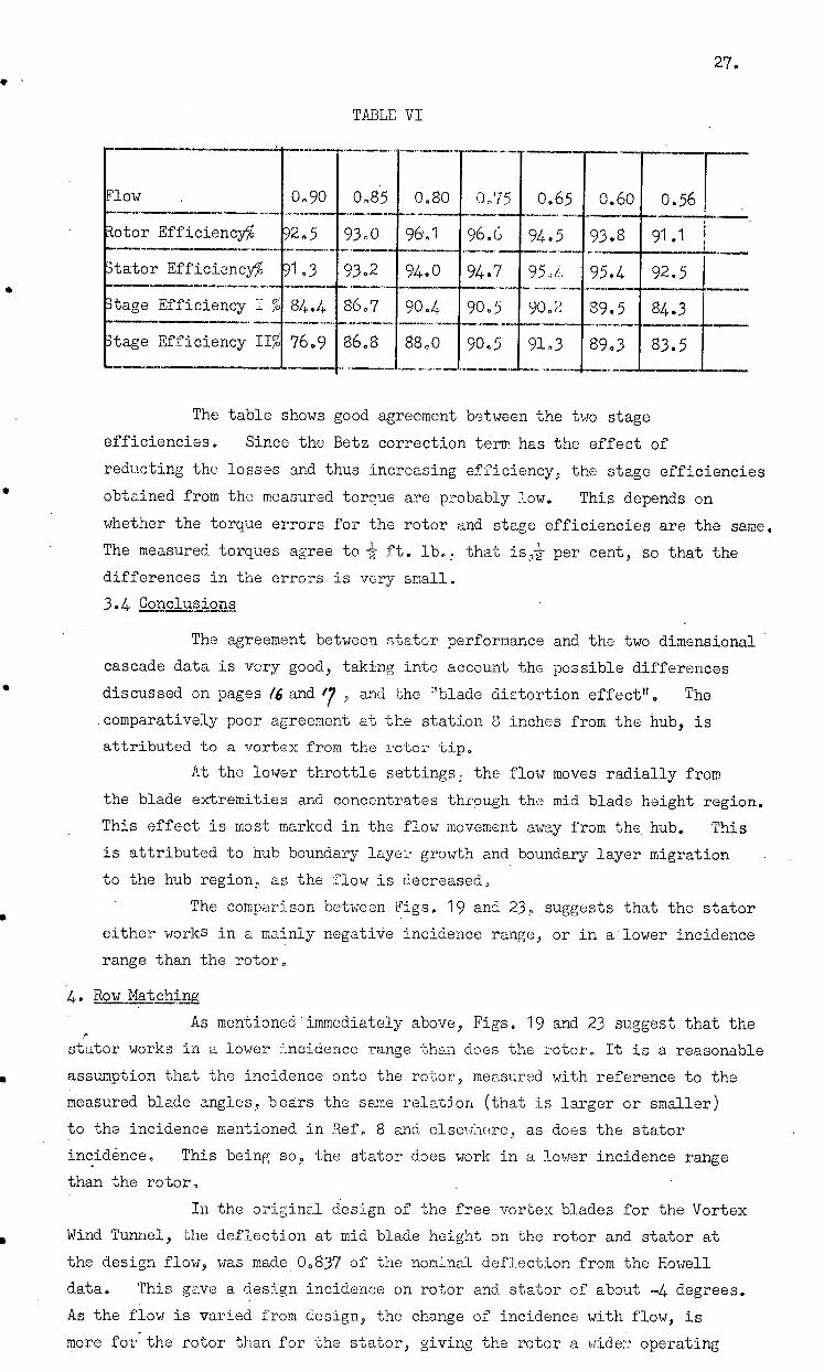
TABLE VI

low . 0,90 0.85 0.80 0.75 0.65 0.60 0.56

otor Efficiency% 2.5

1.3

9300 j961

93.2 j94.0

96.6

94.7

94.5

95,4

93.8 91.1

tator Efficienc A 95.4 92.5

tage Efficiency I cr; 84.4 86.7 90.4 90.5 90.2 89.5 84.3

tage Efficiency II% 76.9 86.8 88.0 90.5 913 89.3 83.5

The table shows good agreement between the two stage

efficiencies. Since the Betz correction term has the effect of

reducting the losses and thus increasing efficiency ; the stage efficiencies

obtained from the measured torque are •probably low. This depends on

whether the torque errors for the rotor and stage efficiencies are the same.

The measured torques agree to ft. lb. : that is per cent, so that the

differences in the errors is very small.

3.4 Conclusions

The agreement between stator performance and the two dimensional

cascade data is very good, taking into account the possible differences

discussed on pages 46 and 7 , and the 'blade distortion effect". The .comparatively poor agreement at the station 8 inches from the hub, is

attributed to a vortex from the rotor tip.

At the lower throttle settings, the flow moves radially from

the blade extremities and concentrates through the mid blade height region.

This effect is most marked in the flow movement away from the hub. This

is attributed to hub boundary layer growth and boundary layer migration

to the hub region, as the flow is decreased,

The comparison between Figs. 19 and 23, suggests that the stator

either works in a mainly negative incidence range, or in a'lower incidence

range than the rotor.

4. Row Matching

As mentioned'immediately above, Figs. 19 and 23 suggest that the

stator works in a lower incidence range than does the rotor. It is a reasonable

assumption that the incidence onto the rotor, measured with reference to the

measured blade angles ; bears the same relation (that is larger or smaller)

to the incidence mentioned in Ref. 8 and elsewhere, as does the stator

incidence, This being so, the stator does work in a lower incidence range

than the rotor,

In the original design of the free vortex blades for the Vortex

Wind Tunnel, the deflection at mid blade height on the rotor and stator at

the design flow, was made, 0.837 of the nominnl deflection from the Howell

data. This gave a design incidence on rotor and stator of about -4 degrees.

As the flow is varied from design, the change of incidence with flow, is

more for the rotor than for the stator, giving the rotor a wide:- operating

28.

incidence ranze. Thus the stator was designed to work at negative incidence

over most of the flow range, Table II on page $ indicates that the rotor

and stator are at neative incidence at design conditions, so that the

performance of the cast blades is in line with the original desi gn.

5. Comparison of Results with_the_Si cascade, Tests

5.1 Presentation and Calculations

Comparisons between the incidence versus deflection curves for

the Si Cascade and the Vortex Wind Tunnel rotor and stator at mid blade

heiht are shown in fi e . 29, The Howell curve for the Si Cascade is also

included. Curves of drag coefficient. C D plotted against incidence, for

the Si Cascade and the stator at mid blade heiht are also presented. The

coefficient of drag was computed by the method duo to A.. Betz, discussed

on page 24

The rotor deflections were calculated from measurements downstream

of the rotor, by assuming the momentum thicknesses of the rotor and stator

wakes at mid blade height to be the same. The assumption that the

displacement thicknesses were the same, made no significant difference

to the calculated deflections,

The results of the Si Cascade tests are given in Ref. 4, but the

actual numbers used to plot the graphs were taken from the calculations

file of the Si Cascade tests,

5.2 Discussion of Results

5,2.1 Discussigh . of_Deflentions

Although the curves of the Si Cascade, and the rotor and stator

mid blade height deflections do not coincide, their gradients are

very similar, The "blade distortion effect" has been assumed to

give deflections, 2 degrees smaller for a given incidence, than those

predicted from two dimensional cascade data, In this case the

deflections are higher by about 2 degrees for both rotor and stator.

The only explanation that can be advanced for this is that the

growth of wall boundary layers through the diffusing vanes, causes

a flow aCceleration, especially throL01 the mid blade height region.

This causes an effect similar to that noted for the rotor hub and

mid blade height regions, on page zz , resulting in increased

deflections. This should not have been present in the low •speed

Si Cascade tests, as boundary layer auction just upstream of the

cascade was employed to give nearly t ,:xo dimensional flow through it.

5,2.2 Discussion of Losses

The agreement between the stator mid blade height and Si Cascade

losses is good. The difference is, at most 25 per cent of the

profile drag which is usually en as 50 per cent of the losses at

a station The losses, as shown by Table Vi on page 2.7 , are as

small as 4 to 5 per cent of the total head ; so that the differences

of 25 per cent in the profile drag coefficient, represent less than

29.

1 per cent of the measured total head, which is the limit of accuracy

of the yawmeter when measuring through wakes, Thus the difference is

negligible.

However, as the stator operating range is within the positive

and negative stalling limits, compsrisons cannot be carried too far.

5.3 LSummary

The performance of the rotor and stator at mid blade height

seems to be close to that of the Si Cascade, Considering the points

of difference between two and three diffiensional cascades, discussed on

page 20 the agreement is very good. The blade distortion effect" cannot

be considered a contributing factor as it should result in lower, not

higher deflections at a given incidence.

The greater deflections from the rotor and stator are difficult

to explain, and the reason offered; that the growth of wall boundary layers

and the resulting flow accelerations cause the increased deflections; is

not convincing.

The most significant feature of the comparisons is that the

deflection curves from rotor, stator, and Si Cascade are parallel to

one another, showina that any difference is constant for sil flow conditions.

6. Comaerison of Results with Previous Tests

6.1 Summary of Results from Previous Tests

• Detailed descriptions of former tests on the cast and machined

free vortex blade sets, are given in Ref. 3, When the tests were being

conducted, the core of the tunnel was open to atmosphere, and air leaked

into the tunnel upstream and downstream of the rotor disk, at the rotor

leading edge and ir inch from the trailisig edge.- Poor overall performance was achieved, the maximum efficiency

obtained with both blade sets bein7 between 70 and 80 per cent, and the

maximum pressure rise being less than 0.6.

A comprison between the stage efficiency and pressure rise

• characteristic's of thc current tests azid the earlier tests of the compressor

fitted with machined blades, is shown in Fig. 30. In the results obtained

during the previous tests, the machined blade set had a slightly better

performance than did the cast blades. For this reason, and also because

it is thought that the machined blades were more carefully set, the machined

blade results have been used for this comparison.

• The total head contours shown in Figs. 32 to 45 are discussed in more detail on pages 38 and 3/. The contour drawn downstream of the

stator, from the preedousseries of tests (Fig. 31.), is compared with Fig. 36

from the current tests, since the flows at which each was obtained, are

nearly the same, The compressor was fitted with a machined rotor and

cast stator when the results for Fig. 31 were taken..

• 6.2 Discussion of Differences BeIllefnarrei_aLTLE.ralls Tests The remarkable improvement of 10 per .cent in efficiency and 25

per cent In total pressure rise, achieved in the current tests is illustrated

in Fig. 30,

30.

The reason for the improvement is suggested by comparing Figs. 31

and 36. The very thick hub boundary layer shown in Fig. 31, which extends

to more thsm 2 inches from the hub, indicates that the hub region of the

stator, and probably of the rotor also, produced very littlework.output.

This thick boundary layer is attributed to the air leak, since it is

difficult to find any other factor or combinetion Of factozs which would

produce this result. Any effects of poor blade setting would be too small

to result in such a large scale and persistent effect, since the thick

boundary layer was observed at all flows in the previous tests,

A. well as rendering the rotor and stator hub regions unserviceable,

the leak also appears to result in the forcirv,:• of the flow through the

remainder of the annulus. Although any accelerations of the flow through

sections of the diffusing rows need not be deleterious, as mentioned on

page 22, the effect of the choking of the flow ne ,lr the hub has been to

worsen the overall row performance, probably because of unsatisfactory

incidence conditions elsewhere along the blade height.

One beneficial result of the air leak has been to widen the flow

range of the compressor. If the flow has been accelerated through the

region away from the hub, then this has presumably postponed stall at the

tip, which Fig. 5 shows is the first section of the blade to stall, and

has resulted in the compressor working at a lower flow.

7. Radial Eouilibrium Stueies

r./1 Presetipu_ancl_Calculations

Curves showing the degree of radial equilibrium attained downstream

of the rotor and stator, are given in figs. 46 and 47. The simple dl.

radial equilibrium condition derived in Ref. 8, is that .)6074.1' = "t/rr

This relation applies only to free stream regions since friction forces,

and any radial flows in the wakes are ignored.

The relation was simplified for computation by integrating both

sides with respect to r giving 11,

A/V // .= Zi( tyir

Integrations are made over finite increments of r which effectively alters the relation to

4 Re /0 1/4,1 .7. 2 044/4 IX- 4

- For the rotor, the static pressure rise Atko14,1 and (KAI )

were computed from the values measured by the yawmeter downstream of the

rotor. in the case of the stator, the free stream values were used.

To plot results, the "radial equilibrium function" E 4 )1. 40, _ 411161C/011

tzra 4 AC./

was introduced, and, was plotted against distance from the hub for each

flow.

Since the radia2 equilibrium function downstream of the rotor is •

•plotted from measu:cements of wake and free stream velocities and pressures,

eq.Tsoddo am_ UT 'mueaqs OGJJ GUq. UT lloTJ Gm_ Jo TUGUIGAOW LI UT q.Tnsal qsnw SO:TM Gm. UT so[; yeTppa Xuu 'mnTaciTTTniDa TuTpua u 7i-Tno Jo meTA Jo TuTod

WOJJ . S9743M UT (i's G:3Pd) J11000 oq umouyi GJP SMOTj TuTpuu

•-2CTdcl.e 4 011 PTP 'Tsuuni puTpl xeq.JoA eug_ Jo Joq.pqs auq q.Tm su °TaTod Tu mom_iq peTeTnoTuo

/4quqoad SPM goTqm '4s 04 wILT-10,TITnbs IPTP13-1 0-EdulTs 0144 11n10114TP ‘ SJTT

PuP 0TTuTV icct peqou SU Tuuqsuoo uTumea TTTm uoTvici .TJTsTp .STTooTen ouT uem.

•wriTaciTITnbs TPTITsa UT sT moTJ -P404 0114 JI • mnTJUTTnbs IT Ti It sq ICPM

MCYET Tvq.oq eLj puu Cq_no seATesmem_ Teouuo I -ETA smaeq_ °sem_ 'JeAerAou MOT; reqoq am_ Jog °TunTaciTunLa reTpuJ UT eq ;OUU70 MOTJ GU°, 'quTod am.

f(7 qt Tem. os 'uoTq.unbe GAOOLP em uT SWJ0q. IR puu , 4%e

'ST Gaud uo ueATS su uoTTo,Jah,, cuIp.:2J em. LIT h OO.IOJ JO uoTTenbe eq.eTdmoo au' °Joquq.s LI u2noJug ST gone moTJ fuTuanT UT pomJoJ 512p1'Lre OJP seoTqJoA

eS@ LiOJ epuTct u Jo mueaq.sumcp sautfl uuu mu,eJ9rs COJj em UT seeTTJoA Jo eouesead OLfl. 2uTuJeouoo uoTssnosTp sT GJOUq_sE puu iO4..se2nd uo

sTEnseu Jo uoTssnosTG

"J09,0MA:Oic

LoTaPuTTL0 s1-14 uP1/4 swomnJorsuT Jailor ° :JuTen 119,nJ em_ LIT peq.dmeq4u ect pTnoo sTuT ToTs TuomnJqsuT UP m.Tm pepTAoad s mTnuue Teuunq em. Jo

TTum Jeqno eug GOUTS e JGAGMOH '1)02:Op:TWO eq qou pTnoo 'sJ,Tsf out de-sTuTV icct pesu SGSJOAPJq os4 Jo -oom.em 'TouunI PUT: X04JOA 9144 JO JOTCp

put Joqoa em. Jo uPeJ;sumou uo -qnqs TUG 1Tuo epuIrJ °Jam sq_soq sy

-ueureq4p ueect

lunTaciTITnbs TPTPP-T qLILq @q-120TPuT oq Lm:r2q- sii TUtiG 0-qc oasm moa ollq Jo meeaqsumop sm.2ueT paouo ;41. put e/T t suoTqnqTaqsTp .74TooTen em_ ;um. ;ouJ

'L °Jou UT ./Tddu qou pTp VJGO, mnTactTTTnbo TuTpuJ e TdwTs 0114 g2n0U4TV °Josseadwoo eaeqs T4Tml t uT Joq.pq_s u Jo tmoaq_sumop sqq2uaT paouo e/T peuTE ,TTu

SLIM mnTaciTTTnbe TuTpuJ q.nuq. punoJ UT SJJ92 puP f_eTuTy

°poor:pa: 4PUMGWOS sT qJJOUIOq.LI9S sTm. Jo

enreA eq; cueAT2 qou sT mnTauTTnbe TtTpua 2uTsTua)oeJ Jo pom.em euq Elf

°M0J am. Jo usaaJ;sumop suquei pJouo e/T q I3 peuTuqp sum mnT J0TITnbs

TuTpua 'epposuo n Uo TEe; II UT Tpuq suoTquem 0L %Toy! uT Jaqauo .6 'jou 11T oq_ poJJeJoa cspom_em u2Tsep ITP Joq.ung.ou, GUMS UT opum osTp sT

uoTqdmnssu sTua, .pemnsu eJu TCJ. euq uloaug_ wemuTuTaJ sTr put ° M0J

°gem u Jo mueaqsdn iiL:TagTTTnbe TuTp .:::J Jo quewuTuq_qu eqq 'seuTuoum moTJ TuTxu Jo u2Tsep or4 ,4. JoJ u9rup a.posuo reuoTsuomTp omq ;73uTsn ui

TicTTT1:TE 75-11MT:17 -77A5TTJTP-Ff-T-6.-i757. TS1-1-5-§Ta • L.

•uoTqounJ 1 euTT-171Paaqs 1 u pomJaq. oq /C:um j0q.Pq.S am. Jo WPGJqSUM0p UOTQDLm GLJI Tum, Os 'uoTquqs 7T1ueJaJwnoJTo e q.P soJnsseJd .

puu SOT4TOOTGA GJP 'puPTI J91440 0U; UO cao^ugs oug. Jo mpoJqsumop pesn senTeA eqj uoTTounJ mnTauTTnbe TuTpuJ 31 -[nct u P pemdeor eq lcum qT

c: eonpoJTuT qsnm sooTqJoA om. 'snIuuut TT LIT quTod uaAT2. P q.V

/ 02Pd Ue pouTuTdx Tocull:_a ouff,

4 _ e "A /Me *DA"' e°eXiie . "1 4 .4%e -4/1 = je4t7)e • /

•Le

32.

direction, with the flow incompressible. However, these flows are small

and so should give only negligible movements in the free stream.

Investigations were made on the stator of the Vortex Wind Tunnel .

to see if the Bernoulli Theorem applied. The total pressure, as measured

at a radial station dcwnstream of the rotor, was compared with the free

stream total pressure at the corresponding station downstream of the

stator. The differences varied from 0 to 10 per cent for the various

stations and flows. The differences were random, and comparing total

pressures at corresponding flow stations, as in Fig-:. 11, made no significant

difference. Since any instrument error would show a systematic difference one explanation for the random difference is that the main stream vortices Dena the stream lines from the axial directio]

A figure in Ref. 16, which is further discussed on page 3S, shows quite

clearly this effect. Since the main purpose of investigating radial

equilibrium is to determine the applicability of two dimensional cascade

data to axial compressors, it is clear that for practical purposes radial

equilibrium was not maintained through the stator. Furthermore, although

the flow may be in "bulk" radial equilibrium, yet the simple radial

equilibrium test at a point should show that flow is not in "streamline"

radial equilibrium.

The curves of radial equilibrium function downstream of the stator

(Fig. 47) show out of balance pressure gradients of the order of .01 to

.05 per inch. The local velocity head varies from about 0.5 to 1 as the

flow increases from J0.56 to 0.90, neglecting the regions adjacent

to wall, that is from 0 to 1 and 8 to 9 inches from the hub, Those

parts of the curves, such as between 1.5 and 4 inches from the hub at

= 0.90, and the curve at = 0.56, are considered sinificant, as 1■•■•

the out of balance pressure gradient is greater than 56 of the local

velocity head. Although this is arbitrarily considered a significant

pressure gradient it is still very . small. The other curves do not show

any large scale effects, the steep gradients being more localised. Thus

the flow, particularly in the mid passage region and with the exception

of that at 0 = 0.90 and 0.56; is, according to the simple test, in radial ow, • equilibrium. -

It is noticeable that in general the gradients become smaller

as the overall flow, and the local velocity head decreases, meaning

'T that at the measuring station the flow at all conditions is out of

equilibrium by about the same amount.

Downstream of the rotor the curves are not so regular as those

downstream of the stator, and local gradients are, in most cases steeper.

mid passage hoever, the curves are Quite flat, with the exception

of the curve at = 0.65. As noted on page Z2, the rotor has stalled,

and this may give rise to the large out of balance pressures, because of

the unstable conditions along the blade. These are shown in Fig. 49, where

the statia pressure distributions is very irregular compared to those

at the other flows.

One reason for the rotor curves showing larger out of balance

pressures than those for the stator may be that the static pressure

.•""

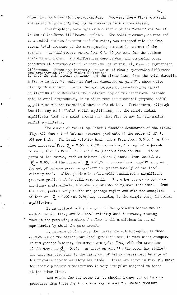
32.

direction, with the flow incompressible. However, these flows are small

and so should give only negligible movements in the free stream.

Investigations were made on the stator of the Vortex Wind Tunnel

to see if the Bernoulli Theorem applied. The total pressure, as measured

at a radial station downstream of the rotor, was compared with the free

stream total pressure at the corresponding station downstream of the

stat. The differeles varied from 0 to 10 per cent for the various

stations and flows. The differences were random, and comparing total

pressures at correspondin flow stations, as in Fia. 11, made no significant

difference. Since any instrument error would show a systematic difference one explanation for the random difference is that the main stream vortices Pend the stream lines from the axial directiol

A figure in Ref. 16, which is further discussed on page 3$, shows quite

clearly this effect. Since the main purpose of investigating radial

equilibrium is to determine the applicability of two dimensional cascade

data to axial compressors, it is clear that for plactical purposes radial

equilibrium was not maintained through the stator. Furthermore, although

the flow may be in "bulk" radial equilibrium,:et the simple radial

equilibrium test at a point should show that flow is not in "streamline"

radial equilibrium.

The curves of radial equilibrium function downstream of the stator

(Fig. 47) show out of balance pressure gradients of the order of .01 to

.05 per inch. The local velocity head varies from about 0.5 to 1 as the

flow increases from = 0.56 to 0.90, neglecting the regions adjacent

to wall, that is from 0 to 1 and 8 to 9 inches from the hub, Those

parts of the curves, such as between 1.5 and 4 inches from the hub at

AL. 0.90, and the curve at = 0.56, are considered sinificant, as m•s.

the out of balance pressure gradient is greater than 5 of the local

velocity head. Although this is arbitrarily considered a significant

pressure gradient it is still very . small. The other curves do not show

any large scale effects, the steep gradients being more localised. Thus

the flow, particularly in the mid passage region and with the exception

of that at 0= 0.90 and 0.56, - is, according to the simple test, in radial

equilibrium.

It is noticeable that in general the gradients become smaller

as the overall flow, and the local velocity head decreases, meaning

that at the measuring station the flow at Rll conditions is out of

equilibrium by about . the same amount.

Downstream of t ho rotor the curves are not so regular as those

downstream of the stato2, and local gradients are, in most cases steeper.

Pt mid passage hoever, the curves are Quite flat, with the exception

of the carve at = 0.65. As noted on page 22, the rotor has stalled,

and this may give rise to the large out of balance pressures, because of

the unstable conditions along the blade. These are shown in Fig. 49, where

the statio pressura distributions is very irregular compared to those

at the other flows.

One reason for the rotor curves showing larger out of balance

pressures than those for the stator may be that the static pressure

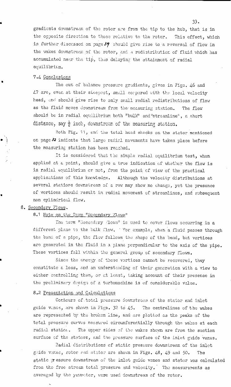
33. gradients downstream of the rotor are from the tip to the hub, that is in

the opposite direction to those relative to the rotor. This effect, which

is further discussed on page .37 should give rise to 'a reversal of flow in

the wakes downstream of the rotor, and a redistribution of fluid which has

accumulated near the tip, thus delayin the attainment of radial

equilibrium.

7.4 gonclp.sions The out of balance pressure gradients, given in Figs. 46 and

47 are, even at their steepest, small copared with the local velocity

head, and should give rise to only small radial redistributions of flow

as the fluid moves downstream from the measuring station. The flow

should be in radial equilibrium both "bulk" and ustreamlineh, a short

distance, say -1-3. inch, 'downstream of the measuring station. Both Fig. 11, and the total head checks on the stator mentioned

on page 32 indicate that large radial movements have taken place before

the measuring station has been reached,

It is considered that the simple radial equilibrium test, when

applied at a point, should give a true indication of whether the flow is

in radial equilibrium or not, from the point . of view of the practical

applications of this knowledge. Although the velocity distributions at

several stations downstream of a row may show no change, yet the presence

of vortices should result in radial movement of streamlines, and subsequent

non cylindrical flow.

8. Secondary Flows,

8.1 Note on the Te rm "Secondary Flows"

The term "Secondary Flows" is used to cover flows occurring in a

different plane to the bulk flow. ' For example, when a fluid passes through

the bend of a pipe, the flow follows . tha shape of the bend, but vortices

are generated in the fluid in a plane perpendicular to the axis of the pipe.

These vortices fall within the general group of secondary flows.

Since the energy of these vortices cannot be recovered, they

constitute a loss, and an understanding of their generation with a view to

either controlling them, or at least, taking account of their presence in

the preliminary design of a turbomachine is of considerable value.

8.2 Presentation and Calculations

Contours of total pressure downstream. of the stator and inlet

guide vanes, are shown in Figs. 32 to 45. The centrelines of the wakes

are represented by the broken line, and are plotted as the peaks of the

total pressure curves measured circumferentially through the wakes at each

.radial static;. The upper sides of the wakes shown are from the suction

surface of the stators, and the pressure surface of the inlet guide Vanes.

Radial distributions of static pressure downstream of the inlet

guide vanes, rotor end stator are shown in Figs. 48, 49 and 50. The

static pressure downstream of the inlet guide vanes and stator was calculated

from the free stream total pressure and velocity.. The measurements as

averaged by the yawmeter, were used downstream of the rotor.

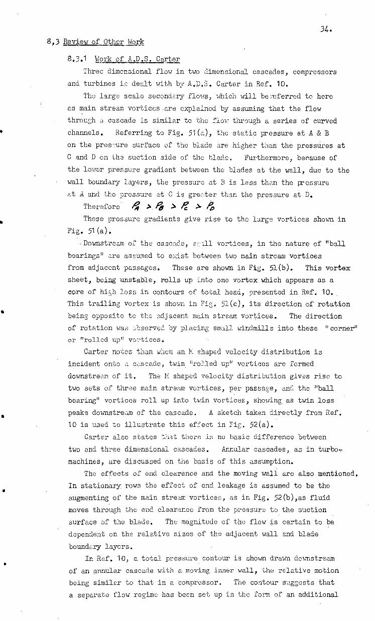
34. 8,3 Review of Other Work

8.3.1 Work of A.D.S. Carter

Three dimensional flow in two dimensional cascades, compressors

and turbines ie dealt with by A.D.S. Carter in Ref. 10.

The large scale secondary flows, which will beeeferred to here

as main stream vortices areexplained by assuming that the flow

through a cascade is similar to the flow through a series of curved

channels. Referring to Fig. 51(a), the static pressure at A & B

on the preseure surface of the blade are higher than the pressures at

C and D on the suction side of the blade. Furthermore, benause of

the lower pressure gradient between the blades at the wall, due to the

wall boundary layers, the pressure at B is less than the pressure

at A and the pressure at .0 is greater than the pressure at D.

Therefore 4 ›.Pg.N

These pressure gradients give rise to the large vortices shown in

Fig. 51(a).

.Downstream of the cascade, Fe:ill vortices', in the nature of "ball

bearings" are assumed to exist between two main stream vortices

from adjacent passages. These are shown in Fig. 51(b). This vortex

sheet, being unstable, rolls up into one vortex which appears as a

core of high loss in contours of total head, presented in Ref. 10. .

This trailing vortex is shown in Fig. 51(c), its direction of rotation

being opposite to the adjacent main stream vortices. The direction

of rotation was bserved by placing small windmills into these "corner"

or "rolled up" voetices.

Carter notes than when an M Shaped velocity distribution is

incident onto a cascade, twin . hrolled up" vortices are formed

downstream of it. The M shaped velocity distribution gives rise to

two sets of three main stream vortices, per passa ge, and the "bp11

bearing" vortices roll up into twin vortices, showing . as twin loss

peaks downstream of the cascade. A sketch taken directly from Ref.

10 is used to illustrate this effect in Fig. 52(a).

Carter also states that there is no basic difference between

two and three dimensional cascades. Annular cascades, as in turboe

machines, are discussed on the basis of this assumption.

The effects of end clearance and the moving wall are also mentioned.

In stationary, rows the effect of end leakage is assumed to be the

augmenting of the main stream vortices, as in Fig. 52(b),as fluid

moves through the end clearance from the pressure to the auction

surface of the blade. The magnitude of the flow is certain to be

dependent on the relative sizes of the adjacent wall and blade

boundary layers.

• In Ref. 10, a total pressure contour is shown drawn downstream

of an annular cascade with a moving inner wall, the relative motion

being similar to that in a compressor. The contour suggests that

a separate flow regime has been set up in the form of an additional

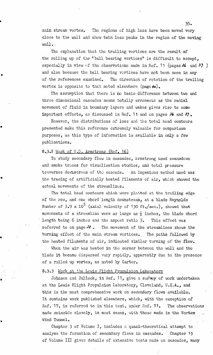
35. main stream vortex.- The regions of high loss have been moved very

close to the wall and show twin loss peaks in the region of the moving

wall..

The explanation that the trailing vortices are the result of

the rolling up of the "ball bearing vortices" is difficult to accept, -

especially in view of the observations made in Ref. 11 (pages34 and 3 7 )

and also because the ball bearing vortices have not been seen in any

of the references examined. The direction of rotation of the trailing

vortex is opposite to that noted elsewhere (page0).

The assumption that there is no basic difference between two and

three dimensional cascades seems totally erroneous as the radial

movement of fluid in boundary layers and wakes gives rise to some

important effects, as discussed in Ref. 11 and on pages 36 and 37.

However, the distributions of loss and the total head contours

presented make this reference extremely valuable for comparison

purposes, as this type of information is available in only a few

publications.

8.3.2 Work of W.D. Armstrong (Ref. 16)

To study secondary flow in cascades, Armstrong 'used swansdown

and smoke traces for visualisation studies, and total pressure

traverses downstream of the cascade. An ingenious method used was

the tracing of artificially heated filaments of air, which showed the

actual movements of the streamlines.

The total head contours which were plotted at the trailing edge

of the row, and one chord length downstream, at a blade Reynolds

Number of 3.9 x 105 (axial velocity of 130 ft./sec.), showed that

movements of a streamline were as large as ir inches, the blade chord

length being 6 inches and the aspect ratio 3. This effect was

referred to on page 32 • The movement of the streamlines shows the

turning effect of the main stream vortices.. The pathe followed by

the heated filaments of air, indicated similar turning of the flow..

When the air was heated in the corner between the wall and the

blade it became dispersed very rapidly, apparently due to the presence

of a rolled up vortex, as noted by Carter.

8.3.3 Work at the Lewis Flicrht proallsion Laboratou

Johnsen and Bullock, in Ref. 11, give a surVpy of work undertaken

at the Lewis Flight Propulsion Laboratory, Cleveland, U.S.A., and

this is the most comprehensive work on secondary flows available:.

It contains work published elsewhere, which, with the exception of

Ref. 17, is referred to in this text, under Ref. 11. The observations

made coincide closely, in most cases, with those made in the Vortex

Wind Tunnel.

Chapter 3 of Volume I, includes a quasi-theoretical attempt to

analyse the formation of secondary flows in cascades. Chapter 15

of Volume III gives details of extensive tests made on cascades, many

36.

being taken from Ref. 17 which showed detailed visdalibation studies:

In Volume I, the equation of forces in the radial direction Ks. Or/ # )1/X — Wt,/ - /c)r • fdr AKE? Ar

is examined, and the assumption is made that static pressures and

their gradients in wakes and boundary layers are neatly the same at

those of the adjacent free streams. ASsuming also that in statot

boundary layers and wakes K and V. are smaller than the free Stteaffi values, and that 6 remains small, the derivatives of 6 and henceitself become significant.

On rotors, Y is larger than in the adjacent free stream, so

that if the above assumptions still hold good, the sign of the

derivatives of is reversed.

The assumption that static pressures in boundary layers and

wakes are nearly the same as in the adjacent free stream is

reasonable, as noted in Ref. 7. The assumptions that k . and &

are smaller in wakes, are all right from the definition of a boundary

layer. However, the as•umption that i5 is small must depend on

factors such as the Reynolds Number of the flow, and whether the

vanes are accelerating or diffusing. In separation bubbles, separated

regions at the trailing edge and thick wakes, 4.* will be much smaller than if the wakes are thin, and so it is in these regions that

radial boundary layer flows may be expected to occur. This is supported

by photographs of paint traces on blades which are discussed on page 37 .

Once the idea of flows within boundary layers and wakes is

introduced, the possibility arises that regions of high loss, such

as those near the walls are Caused, at least in part, by the transport

of low energy fluid from elsewhere. This is easy to understand in the

case of stators, as low energy air from the blade pressure side moves

down the wall through the boundary layer,. and collects in the corner

between the suction surface and the adjacent wall. This is discussed

on page .37.. Observations in Vol. III show that the movements in rotor boundary layers are rather more complicated.

Reference is made in Volume I to tests on an axial flow compressor

where, at.a radial station, the efficiency of the stage was higher A than that of the rotor. If the flow is wholly cylindrical, then

the efficiency of the stator is more than 100 per cent. The logical

reason for this, apart from measuring error, is that low energy air

has been moved from the radial station on the stator, so that losses

do not appear at that station.

In Volume III observations of secondary flows in two and three

dimensional cascades are shown, including the cases of tip leakage

and the moving wall. The migration of fluid in the wall boundary

layers, from the pressure to the. suction of the channel, and the

consequent rolling up of this fluid into a trailing vortex similar

37.

to that noted by Carter, and in the manner shown by vortex A of

Fig. 53 (a), is demonstrated. The size and vorticity of the vortex

increased with the air deflection. The direction of rotation of the

vortex ais, however, - opposite to that shown by Carter, being in the

same direction as the adjacent main stream vortex.

Contours of loss of kinetic energy, drawn downstream of an annular

stator, show twin vortices in the region of the hub, rotating in the

direction shc:Yn by vortices in Fig, 53(a). The two loss regions are

similar to the twin loss peaks noted by Carter in Ref. 10 and reproduced in Fig. 27. The relatively high loss near the hub as

compared to the . tip, is attributed to boundary layer movement giving

a similar effect to that mentioned on the previous page where the

stage efficiency at a radial station, was higher than the rotor

efficiency at the same radial station.

The movement of fluid in blade boundary layers, is shown by

photographs of paths taken by paint smeared on stator blades. The

paint traces moved radially inward from the tip to the hub along two

'paths, one near mid blade height and the other at the blade trailing

edge. The path near mid blade height is most likely to be through

the separation bubble, since the friction forces there and in the

separated region at the trailing edge, should be lower then elsewhere

on the blade.

Tests on a two dimensional cascade with end clearances of 0.4

and 1.7 per cent of the span, show migration of air from the wall

and blade boundary layers on the pressure side, through the end

clearance to the suction side. This air formed the inner of twin

vortices, similar to Vortex A of Fig. 53(a). The end clearances in

the Vortex Wind Tunnel are given in Table III , page 9 , and are of

the same order, being within the range 2/3 to 2 per cent of the span.

The effect of a trailing vortex from one rOhleon the downstream

row, is shown by photographs of smoke traces which indicate separation

occurring on the downstream row, where it was struck by the vortex.

8.4 Discussion of Secondary Flows in the Vortex Wind Tunnel

8.4.1 Conditions in the Vortex Wind Tunnel

For a clear understanding of boundary layer movement in the

Vortex Wind Tunnel, it is necessary to examine blade surface

pressures, especially those on the rotor. In 1958 measurements

of blade surface pressures were made on rotor and stator blades

of the machined free vortex set. No tapped blades of the cast

set are available. Also the tests were conducted with the air

• leak at the rotor hub, present. Thus, the test conditions differ

from those under which the current tests were conducted. .

However, since general trends only are being looked for, this

should not prove any drawback.

38.

The tendency was for the radial surface pressure distribution

to decrease towards the shell on the rotor, and towards the

hub on the stator. The gradients decreased for radial lines

closer to the trailing edge. However, pressure peaks and

troughs were noticeable and these must be of prime importance

because of their influence on thel.../Dterm in the force

equation in the radial direction. It is to be expected that

pressure peaks and troughs will be more frequent on the surface

of the cast blade set because of their irregular surfaces.

The curves of static pressure, downstream of the blade rows shown in Figs. 48 , 49 and 50 show that the gradients are very definitely from the tip to the hub downstream of the rotor, while

downStream of the stationary rows the gradients, while being

generally in the same direction, are not nearly so clearly

defined. .

8.4.2 Secondar -r Flows Induced by Stator and Rotor

Two interesting phenomena shown in Figs. 32 to 36, suggest

the iresence of twin vortices neat the hub.

(i)The wake centreline. near the hub is distorted in a manner

which can be satisfactorily explained by the presence of twin

vortices, the inner near the wall rotating in the clockwise

direction, and the outer in the anticlockwise direction. This

is similar to the effect noted in Volume III of Ref. 11, and

discussed on page 37 . The distortion of t he wake centreline

due to twin vortices is demonstrated in Fig. 53(c).

(ii)A core of high loss, smnller than that near the hub,

seems to exist further away from the wall. In Fig. 36 a

small loss core was actually measured, although this may be

instrument error. However, the second loss peak near the

hub shown in some of the curves in Fig. 27 supports this.

Althoush yawmeter measurements near the wall are certainly

in error to Some exteA,-y9t the centrelindistortion is to

marked, and agrees so well with Johnsen and Bullock that the

phenomenon cannot be dismissed as due to the method of

instrumentation.

At the stator tip thre is no sign of twin vortices, and the

vortex present, seems to have little effect in distorting the

wake centreline.

The contours in Figs, 32 to 38 show that the local strength

of the vortices decrAases with decreasing flow, that is, with

increasing lift and pressure difference across the passage

between the blades. This is apparently opposite to the effect

discussed in Ref. 11 and noted on page 37 . The contours at

0S_ 0.60 and 0.56 show little sign of twin vortices near

the hub. There may be no conflict however, between the

observations by Johnsen and Bullock and those in the Vortex

Wind Tunnel, as, on the total pressure contours, the vortices

having high local vorticity show up most clearly. The vortices

at # = 0.60 and 0.56 which are large, ray have hi7.her overall 4.6v vorticity although they are not so localised and therefore, not

so easy to see.

A comparison between the contours downstream of the stator

and the corresponding curves of $6 and 4; (Figs. 24 and 25) shows

that a knee in the radial distribation curves near the hub )

coincides with the join between the wall boundary layer and the

adjacent blade wake. In this context, the wall boundary layer

includes the hub vortices. The position is similar at the tip,

and the knee in the curves ofgy and Vi in the case of the ah.; - stator, is a good guide to the extent, in the radial direction )

of the secondary flows in wall boundary layer and wake.

Downstream of the rotor the only curves available are the --

distributions ofand C(Figs. 21 & 22). Assuming that the

static pressure gradients on the stator, which run from the

tip to the hub, caused the concentration of secondary flows

near the hub, it seems reasonable to expect a similar concentration

at the rotor tip. However, this is not indicated by Figs. 21 and

22, where the knee in the curve near the tip, is much closer to

the wall than is the case near the hub. This may be caused by the

high energy of vortices from the rotor tip which are shed with a

velocity component in the circumferential direetion ) . 4 •

This must .=4-ive a deceptively high total head reading on the

yawmeter. also, the static pressure gradient downstream of the

rotor, which runs from the tip to the hub should result in the

redistributing of low energy air in the wakes, after it had

collected in the tip region while passing throudi the rotor

itself.

The effect of the moving wall at the rotor tip and for

some part of the hub, as in Fig. 2, makes a detailed discussion

of secondary flow formation in the rotor impossible with the lack

of suitable measurements, and this will not be attempted.

8 24 2 3 2 Secondary Flows Induped_12y Inlet Guide Vanes

The contours of total head downstream of the inlet guide

vanes are shown in Figs. 39 to 45. The static pressure

distributions in Fig. 48 show that the gradients tend to run

from the tip to the hub, as on the stator. On the inlet guide

vanes there is no separation bubble, there are thin wakes and

boundary layers, and only a small separated region near the

trailing edge. Thus any radial boundary layer and wake flows

are restricted because of lack of suitable pathsand high

friction forces, as compared to the stator. This possibility

has already been mentioned on page 34 .

40 .

The contours show wake centreline distortion, both at the

hub and tip, consistent with twin vortices in those regions.

The cause of this is likely to be the restricting of radial

boundary layer flows, so that the inlet guide vanes are similar

in this respect to a two dimensional cascade.

The thinning of the wake at about 1 inch from the hub, which

is also present in the contours downstream of the stator, may

be caused by the energising of the wake by the edge of a fast

vortex, or may indicate the presence of a pressure peak causing

wake fluid to move away from that region.

8.5 aiggested Picture of Secondary Flow Formation

8.5.1 Different Secondary Flow Formations

To obtain a clear picture of secondary flow formation

a subsiduary experiment was undertaken. A small water

channel, shown in Fig. 54(a) was used. It is fitted with

a gate which is flush with the side walls. The height of

the gate was adjusted to give a much greater depth of water

on the upstream side of the gate than the downstream side.

The pressure aradientS in the upstream part of the water

are similar to a bend in a pipe, and to the flow through

an aerofoil cascade, as the water must turn to pass under

the gate. Two large mainstream vortices, similar to those

noted by Armstrong and Carter, could be seen and are shown

in the photograph in Fig. 54(b). Their distance from the

gate varied with water surface disturbances, but when they

moved an inch or more away from the gate, ink fed into

the corner between the gate and the wall showed the presence

- of small vortices in the corners.. One can faintly be seen in

Fig. 54(c) indicated by the arrow A.

The direction of rotation of the corner vortex was the

same as of the main stream vortex; that is, opposite to the

direction of rotation noted by Carter, but the same as noted

by Johnsen and Bullock.

3ince the tests on the cast free vortex blade set have

been completed, persloex windows have been fitted in the

outer annulus walls of the Vortex Wind Tunnel. Tests

at very low rotor speeds using smoke were attempted, and

these tests, although inconclusive, suggested that twin

vortices rotating in the manner suggested by the total

head contours, exist through, and downstream of, the stator

hu'rexegion.

A summary of the somewhat conflicting data on secondary

flow formations is now given.

In the Carter two dimensional cascade tests, and in the

water channel, there was only one vortex in the corner.

Loss contours shown in aef. 17, exhibit wake centreline

41.

distortion siMiler to that in the Vortex Wind Tunnel

contours, which sugAest the :Presence of twin vortices. This

idea is. reinforeed somewhat by the smoke trace tests

mentioned immediately above. Smoke tests shown in Refs.

17 and 11 show a vortex close to the wall formed by air

moving in the wall boundary layer, from the pressure to the

suction side of The blade space and there, rolling up. The

direction of spin of this vortex was opposite to that noted

by Carter, but the same as the corner vortex in the water

channel.

An attempt will now be made to sort this into a coherent

picture of secondary flow formation.

8.5.2 SecondarI_Flow Formation

As a fluid moves through a two dimensional cascade, the

pressure gradient across the blade space causes the formation

of main stream vortices similar to those shown in Fig, 51(a).

This pressure gradient also causes fluid in the wall boundary

layers to move from the pressure to the suction side of the

channel as shown in Ref. 17.. When it reaches the suction

surface, there is no spanwise pressure gradient to move it

along the blade and it rolls up into a corner vortex, as

shown by the path taken by fluidAin Fig. 53(a). The

direction of rotation of this vortex is the same as the main

stream vortex, and is also the same as the corner vortex

shown in Ref. 17.

The reason why the direction of rotation of the corner

vortex noted by Carter, is opposite to that in the water

channel, is thought to be because the vane used, extended

into the main stream vortex. This would give it a direction

of rotation opposite to that of the main stream vortex.

When, as in the case of an annular cascade, a spanwise

pressure gradient is superimposed on the normal cross channel

gradient, fluid will move through the pressure surface

boundary layer, separation bubble, and trailing edge region,

meet the fluid which moved down the wall and roll up in the

manner of Vortex D in Fig, 53(a). The relative sizes of

these vortices depends, of course, on the magnitude of the

pressure gradients, the size of the separation bubble and

the thickness of the boundary layers.

If there is blade end clearance then there is likely to

be reinforcement of vortex A.

Downstream of the blade row, high pressure air from

that part of the wake from the pressure surface, is adjacent

to low pressure air from the suction surface. The movement

of air in the wake should then be as shown in Fig. 53(b), with

. 42 .

a reinforcement of both vortices in the case of an annular

cascade, and the formation of vortex B in a two dimensional

cascade or inlet guide vane row. The formation of vortex

B is due to the tendency of the fluid to distribute energy

evenly, as is the case when laminar flow bec9mes turbulent.

At the tip of the Vortex Wind Tunnel stator, it seems

likely that no vortex similar to vortex B of Fig. 53(a)'has

been formed. Since the pressure gradient across the annulus

is from the tip, any air moving into this region from the

high to the low pressure side of the wake, will form either

a very weak vortex B or willall be bled away towards the

hub. The reason why vortex A at the stator tip is so

weak compared to the correspondin vortex at the inlet

guide vane tip is probably due to a bleeding away of air

from it under the influence of the spanwise . pressure gradient

Thus twin corner vortices should be formed downstream of

all two dimensional cascades, and at the wall of an annular

diffusing cascade when the wall is the lower end of a

spanwise pressure gradient. At the other wall of an

annular cascade the vortices, if two are present, are weak,

as air will be bled away from them under the influence of

spanwise pressure gradients.. Because of the thin boundary.

•layers and wakes and the absence of a separation bubble,

accelerating cascades 5. rform in a similar manner to two

dimensional cascades,

The presence of main stream vortices, rotating in the

manner shown in Fig. 51(a) is undisputed, although they have

not been seen or measured in the Vortex ijind Tunnel.

8.6 Conclusions on Secondary_Flows

The picture of secondary flows presented in the previous

section fits all the available data, apart from that due to

Carter, which is the earliest work of those examined.

The blade surface pressure gradients discussed, show only

t;

general trends, and it seems obvious that pressure peaks and

troughs on the blades must play a significant part in the

magnitude and direction of boundary layer flows.

Plans for the use of visualisation tests in the Vortex

Wind Tunnel, and the examination of boundary layers and wakes

with small arrowhead ,Tawmeters, are in hand. These measurements

coupled with the normal cylindrical yawmeter traverses and

blade surface pressure readings, should enable the picture of

secondary flows to be clarified.

9. General Conclusions

It seems clear that cast compressor blades should give satisfactory

performances. The difference between the blade profiles and design,

43. and the measured blade angles not being those referred to in Fig. 3, are

drawbacks when comparing the cast blade performance with two dimensional

cascade data. However, any blade distortion has not resulted in any

serious mismatching of the Tows nor seriously reduced the pressure rise

and efficiency which might have been attained had the blades been of design

shape.

The prformance of the compressor rows is close to that predicted

from the Howell data, deflections being with a few exceptions, lower by 2

degrees or less.

The air leak at the rotor hub is the obvious cause of the poor

performance achieved in previous tests. Errors in blade setting would

produce only small differences.

The agreement with the 81 Cascade results is ouite good, the

deflection against incidence curves for the rotor and stator at mid blade

height and the Si Cascade, being within 2 degrees, and the curves are

parallel. However, the cascade results are lower than those measured

in the Vortex Wind Tunnel and the explanation given is rather inadequate.

The flow downstream of both the rotor and stator is,nearlY;.. in

radial equilibrium at the measuring stations. The simple radial

equilibrium test as set out in Ref. 8, should, when applied at a point,

as in the free stream downstream of the stater, give a true indication

of whether, for practical purposes, the flow is in radial equilibrium.

The explanation of the formation of secondary .flows, based on

flows in boundary layers and wakes, adequately covers the data available,

although it is clear that the knowledge available is inadequate.

REFERENCES

44 •

P.V. CROOKS AND U. HOWAD

2. A.W. WRIGHT AND E. SZulAN,J.KI

D.A. FRITH, P. 2UNY.divITYA AND A.R. OLIVER

E.G. BLIGHT AND W. HOARD

*Preliminary China Clay Tests on Rotary Cascade Blade Surfaces". Department of Supply. A.R.L., Note M.E. 196, December 1954

"Calibration of the Vortex Wind Tunnel". Department of Suppy. A.R.L. Tech. Memo. M.E. 165 October 1956

"Initial Testing of 04 Blades in the Vortex Wind Tunnel". Department of Supply. A.R.L., Note M.E. 230, December 1958

"Tests on Four Aerofoil Cascades". Part I, Deflection, Drag and Velocity Distribution". Department of Supply. A.R.L. Report E.74 July 1952

5. R.C. PANKHURST AND "Wind Tunnel Technique". D.W. HOLDER Pitman 1952.

6. A.R. HOWELL •

7. H. SCHLICHTING

8. F.G. BLIGHT

J.H. HORLOCK

10. A.D.S. CARTER

"Fluid Dynamics of Axial Compressors". Proc. Inst. Mech. Eng. Vol. 153, 1945.

"Boundary Layer Theory". Pergamom Press, 1955.

"An introduction to the Aerodynamic Theory of CompreSsors and Turbines". C.S.I.R. Division of Aeronautics, Report E 56, May 1947

"The Compressible Flow Through Cascade Actuator Disks" The Aeronautical Quarterly, May

1958

"Three Dimensional Flow Theories for Axial Compressors and Turbines" Proc. Inst. Mech, Eng. Vol. 159.

11. IRVING A JOHNSEN "Aerodynamic Design of Axial Flow Compressors" and Volume I and III N.A.C.A., RN, E56B03 and

ROBERT O. BULLOCK E56B03b.

"Analysis of the Ar Flow Through Four Stages of Half Vortex Blading in an Axial Compressor". A.R.C. Reports and Memoranda No. 2383 1946.

12. D.G. AIN= AND R.A. JEFFS

•

45. REFERENCES (Contd.)

13. A.R. HOWELL and

R.P. BONHAM

"Overall and Stage Characteristics of Axial Flow Compressors" Proc. Inst. Mech. Eng. Vol. 163

"Tests of a Model of One Stage of the 14. A.R.OLIVER, W. HOWARD New Compressor of the Variable Pressure

and Wind Tunnel".

P.V. CROOKS Department of Supply. A.R.L. Note, M.E. 228, October 1958.

- "The Low Speed Performance of Related 15. A.D.S. CARTER

Aerofoils in Cascade" N.G.T.E, Report R 55.

"An Experimental Investigation of Secondary 16. W.D. ARMSTRONG Flow Occurring in a Compressor Cascade".

The Aeronautical Quarterly. August 1957.

17. HOWARD Z. HERZIG, "A Visualisation Study of Secondary Flows

ARTHUR G. HANSEN

in Cascades" and GEORGE R. COSTELLO

N.A.C.A. Report 1163, 1954.

•

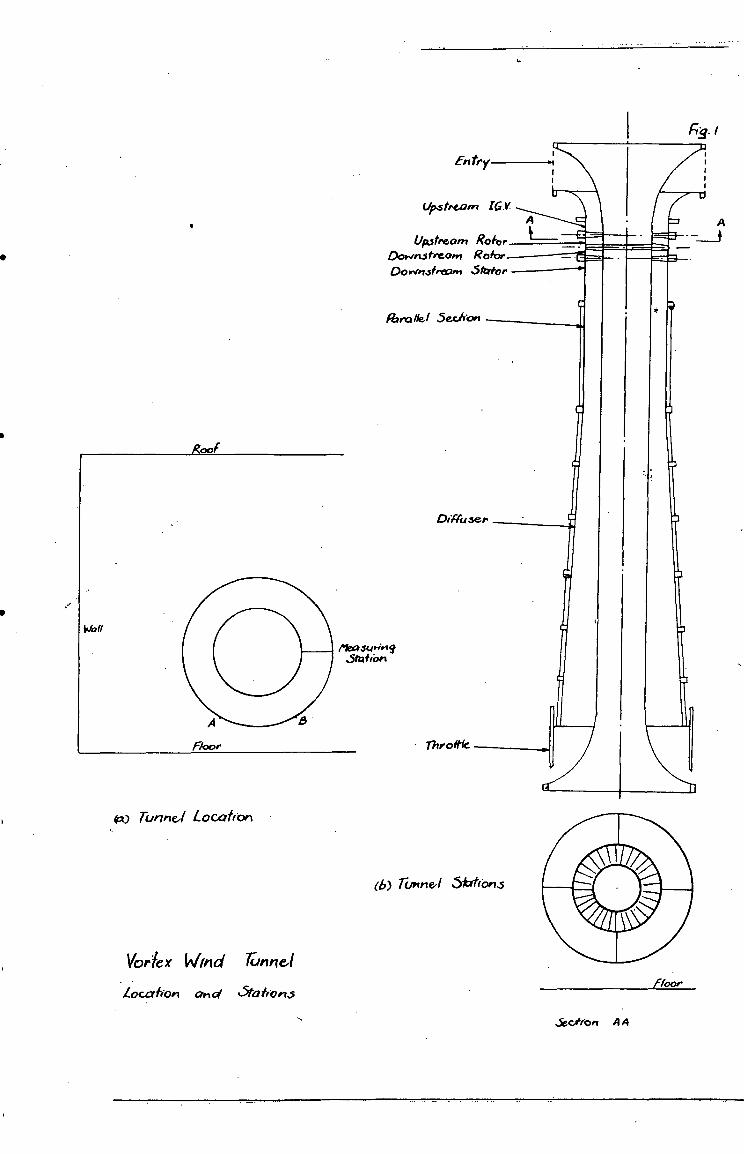
(6) Tonne,/ Statrons

floor

4:0 runne,1 Location

Vorlex Wind runnd

Location arta StairOris

Entry

Upstream EGY

Upstream Ro Fe r

Downstream Redo, Downsfreon, .5/41.0

(broth( Sechon

Chic& se r

• Throttle

Searbrt A A

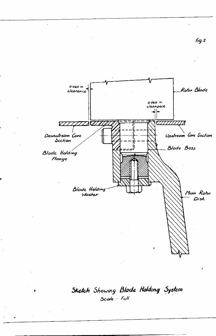
69. 2

Sketch Shotony Blade Holding y$ fern

5ccde Full

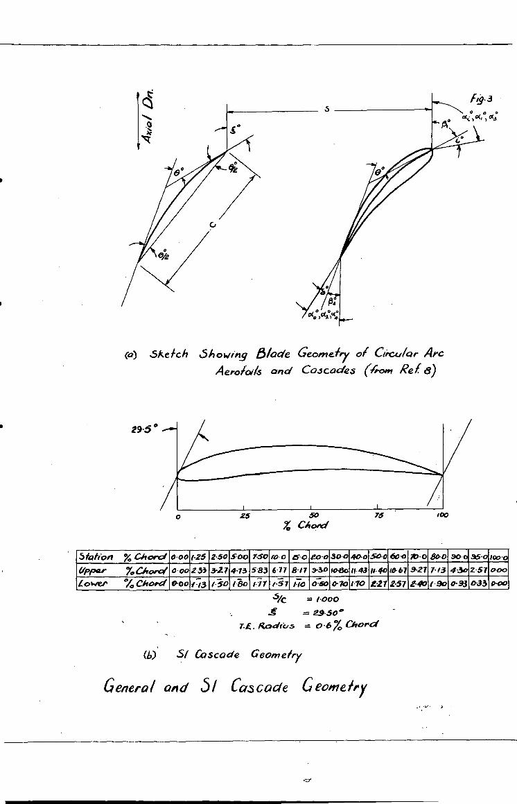
60-o AS-0 0

2-57 1440

80-0 90-o 95.0 100 -0

7.13 4-30 2-57 000

.90 0-93 9-33 0-00

(o) skeich Showing 5/ode Geonleirr of Clic-444w. Arc

Aerofoils and Cascades (loom Rel. 8)

Station chord 0•00 1.25 250 1-50 10-0 45, 0 eo.o 390 40-0 50-o

Upper 70C4ord 0-00 2-33 3-27 4-73 5 -83 6.77 917 9-30 fo-8o n-43 11- 40

Lower %Chord 0-00 113 (-30 1-80 1•0 0750 0-70 110 £21

= 1-000

= 2.9-50 °

7:4 . Radii is = 0 6 X, Chord

(h)' S/ Cascade Geotnehy

General °Ad 51 Cascade C eome/ry

-

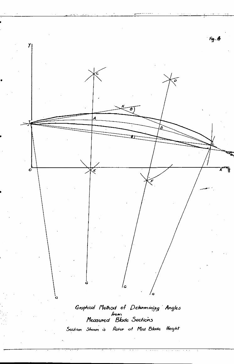
65.4

Graphical MAW of Peleprn4117,9 " Angles /rein

Pleasured 8hde c5eatio;v3

Sechbn Shown Rol-or of Pird bk2de Height

• • • .... •• •• ...... •

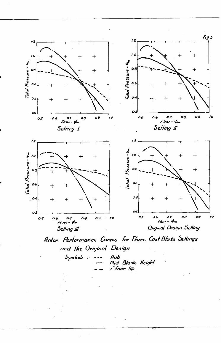
0-6 0.7 06 Row-

Selliny I

0.5

1.2

10

02

0-6 0 7 06

Setting Z

09

1.2

04

02 0 9

04 0-6 01 04 HO &V ". APT

Selling II

0.9 to 05 0-6 at

fkw- 05. Original Design Selfaig

Rotor Performance Curves for Tiiree Cos/ Blade 5elfmgs

and Me Original Design

Sym 604 - - Huh Mid &ode 1410)4

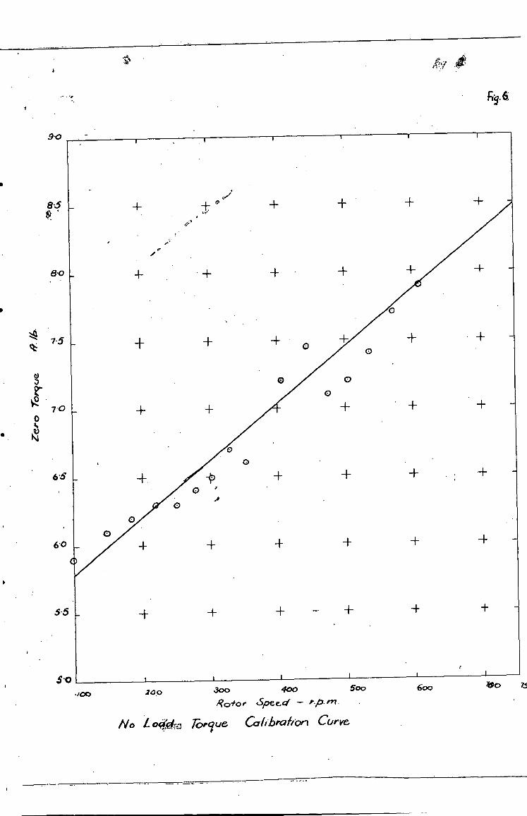
600 .3oo 400 600

R &or Speed - ^p.m.

No L (44 Torque Calibration Curve

F. 6

/00 200

■•• •••"'

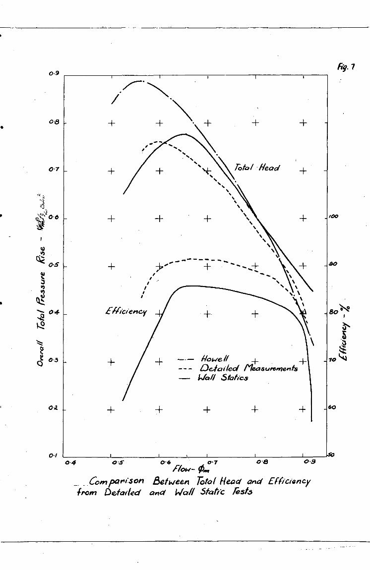
;17-

•••

Efficiency

0-9

0-

0 . 7

0.3 — — I/owe /I 4- A4 . Deiaited /7w/summery& Wall Statics

100

ao

so

70*C64•1

60 02

0.1 0 -4 0 -5' 0-6 0- 7 0 -8 0-9

RON- 0,“

Co in pare/son Between rotot Head and Efficiancy from Detailed ana Wall Static ksts

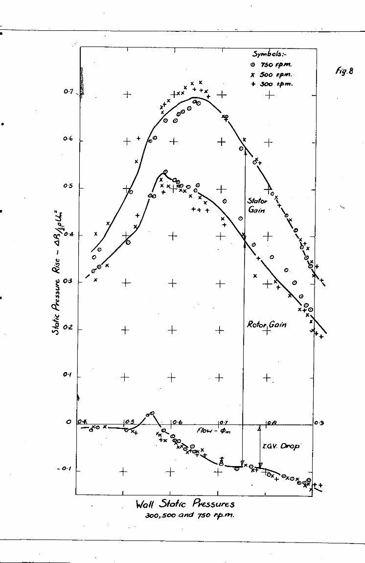
Ut

0

0

0

I " ■

4.c 6c)

`4

. .+

4.5/

atic

Pre

ssur

e R

ise

— 4

8/10

(4, 2

oat

s;•

9

9 0

th

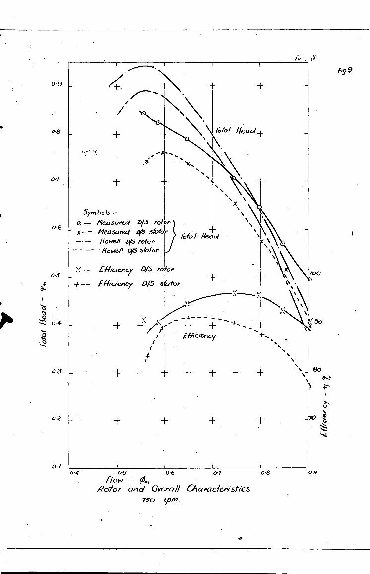
Fry.9 0 . 9 -F

■ NT •

\\

\.;to I !lead +

sx,

0•1

Sy*, 6O LS ---

0 — o- Msed eaur DIS no r }

led e x-- measured 45 sfoior

rota / 'a --- If owll 4/5 to/c" Howe /I ()is Stator or

0%5 0/5 rotor

+ fficie.ney 4/5 sbtor

/00

o.) 0.4

•

0-3

02

V

-I- -.... I%

f ?o, / 4 1C(c/0.4.1 cy

/

/

_

0 o4- 05 06 0-7 0-8

flow - Rotor arid Overall CharacieristiCs

750

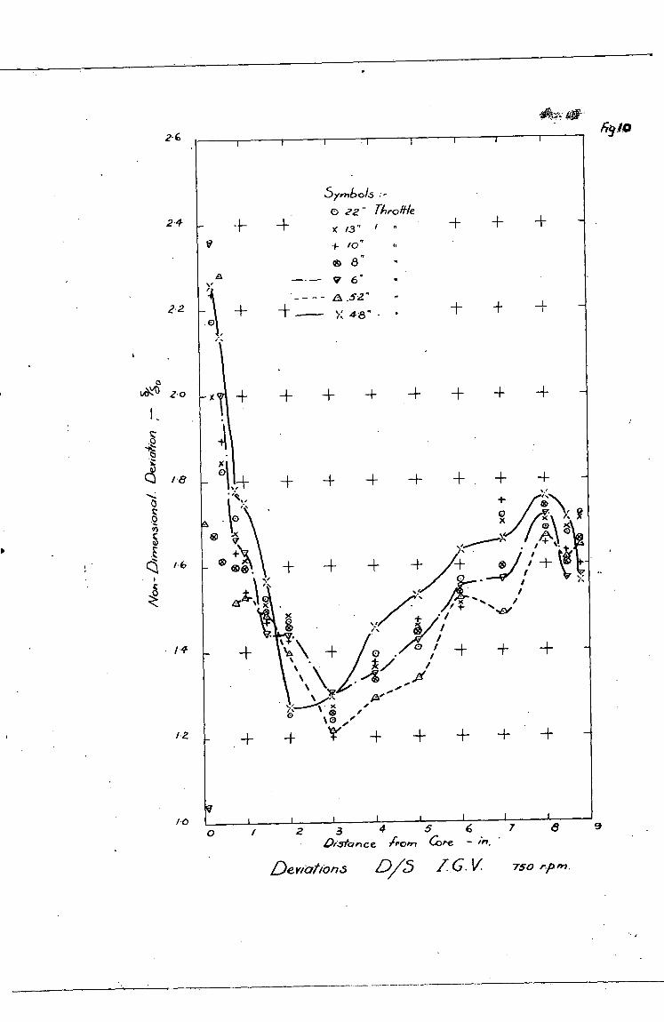
24

22

0

tAzi\'41 2.0

z

CS

z 0

5 , 6

8

'4

2 3 4 5 6 7 8 9

Disto ce ?from Core -

Derkition D/5 I. G. V 750 "ptn.

.0

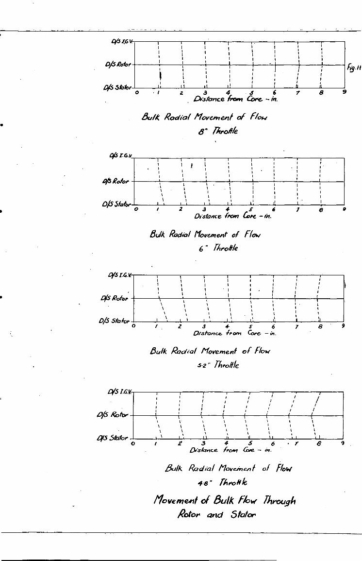
0/5 Rotor

1:G.11 a 1 I i • T I I I I I I I I I i I I I I I I I I I I I

a I I I I I 1 I I ■ I

/ 1 I

I I 4 I } I I I I I I I I I I I I i I I I I I I I I I I I I I

II It I I. 1 I II h 2 a 4 6

D.:stance from Core - in. 7

F6.11

9

• &a Radial Move.pren/ of f-60.,

er Thronk

46 r.G.v.

*Rotor

DIS Stator 0

1

a I t 1 I I 1

I I I I I I I I I I 1 \ 1 a I a I I I I Ii

1 .3 4. 6 Distance from UPC —fit.

7

0

als Rotor

075 14.1!

staiop 0

ices 1.6v

LYS Rotor

.5Clor

Bul4 Radtal Movement of Flow

6" Arolle

I 1 I I r I I I I I I I I I I I I I I I I I I . I I

I I ; I I I I I I I I a t• I a 1 I I tt 1 t 1 t I 1 a 1 1 1 t 1 1 t ti t

1 t t i I I , I I '. I,

2 .3 4. 5 6

7 as fiance Iron, Core -in.

iLlk Radial Movement of POW

5-2" Thtiollie

I I I i I I I I / I i /.

1 I / I I / / i I / I / / / I I r

I I 1 I I

I I \ / ( /I / f , I. , , , , 1 1 \ 1 1 1 I 1 1 1

\ 1 I a I I 1 1 I 1 1 1

9

0 Z 3 4 5 Dishnce frost? Com - en.

r 8

Bak Radial Movement of flow

4e- TApoi

Movement of Bulk flow' Aroygli

Rotor and Stator

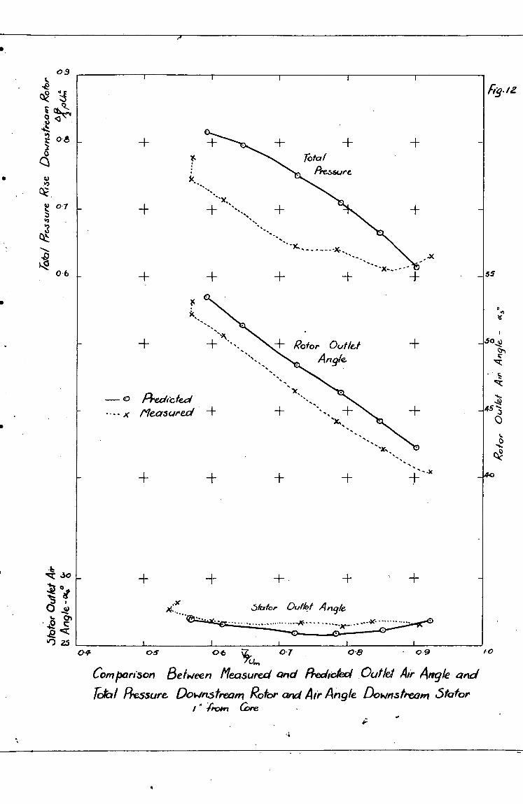
0-9

eb'VN; 113 -

0•8

ks.3

0 6

041 05 0 6 07 08 7u,„

Corn pan .5 on Between Measured and Fiecireted Outlet Arr. Arrysk and

rota, Pressure Dokinstrearn Rotor and Air Angle Downstream 5totor Aviv; awe

t 0 0•9

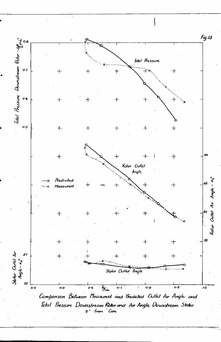
0-4 0-6 o9 0-7 0-8

•

f;:g./.3

•

—0 I:h&c-teal Pleasueeo1

t;

7

Ouilei Atigle

27

newt...7

Comixirison Between ileasureol and tredkted bald Ai Angle, an

rota I g4essure Downsfream loft:).- and Ai. Angle, Downstream Stator are

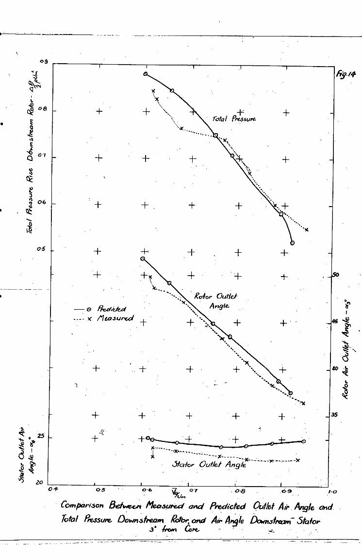
0-5 0•6 -4,, 0.7 . 0,5

Comparison &Asst." Measured and Predicted Paid Atr . Angle 47nd. . Total fiessure Downstream Rotor, and Ali' 111Vie Dcornstrorzin- Stator

3 4 Avon Owe, •

1-0 . 0-9

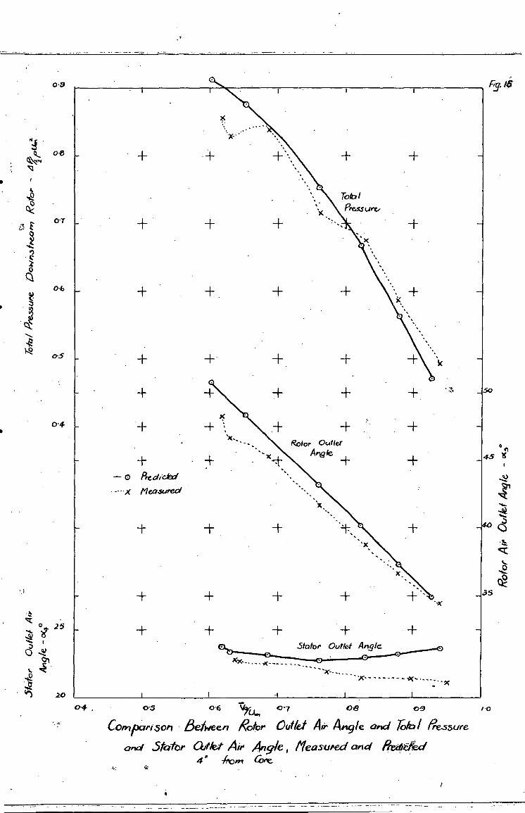
Fi8

50

e n 45

Sta

tor

0(1

10 A

ir

q 08

°25

04

06

07

20

+

-F ROtor Out let

+ —o Prcayc&1

X f1eQ,sureO'

H- + -1- +

* + + -1-

I •

+-

04 03 06 07 0S

ConyJalv'30F1 Be/ea Rotor Out/el Air 419k o'id T0/è1 &55ure

o'id 5fator Olki Air ,4.ig/e, Measued a'ici H&i 4 fl

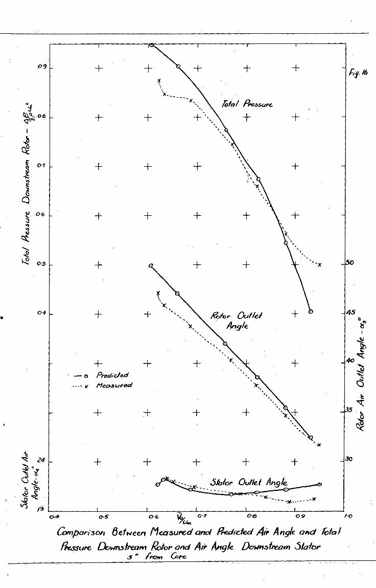
0-9

Ql 4 .0-8 c:J

J 0.1 0-6

r•■

0 -5

0-4

0-4

0-s 0•6 cia, 0 - 7 0-8 0 9

/-0

Comparison eh een Measured and Ppecticted Angle and Tidal

&mute Downstream Rotor ond 40. Angle Downdrearn Stator .5" from Gee

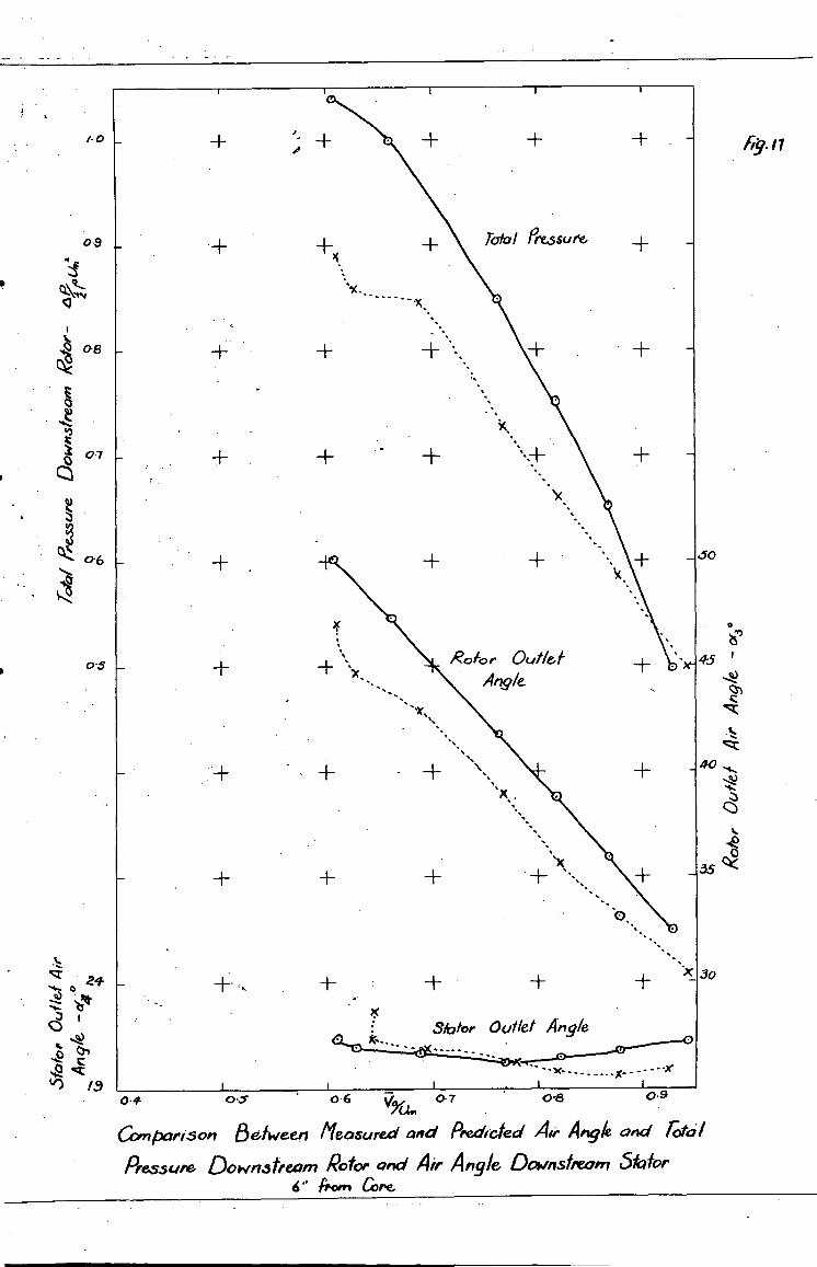
/. 0

05

0.4t OS 0-6 Vya 0.7 0'8 0-9

Comparison Between Measured and Predicted Ali' Angk and rota'

Pressure Downstream Rd°, and Air Angle DOWITSfreelr7 5hior 6" from Core

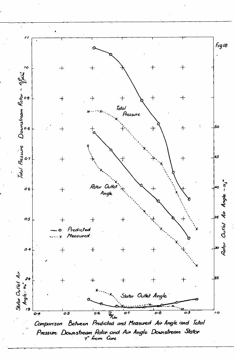
o 8 04 0-5 0-6

-+ A

_ 25 ^

'x\ s, &atop Outlet Angle

/-/

0-4

Comparison &tweet! Predicted and Measured Air Angle and rofal

Pressor, DownstPeam Rotor and Air Angle DOW11 stream Stobr 7" AO Pri COIne

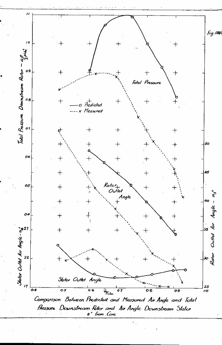
0-6

0-8

09 '

Compart,son E3daveeti Pretirete4 and MeasuPed Angie and &al

assure Downsr"cam Rotor. and 46. Angle Down5treani 5kdoti

e' Awl 6),e

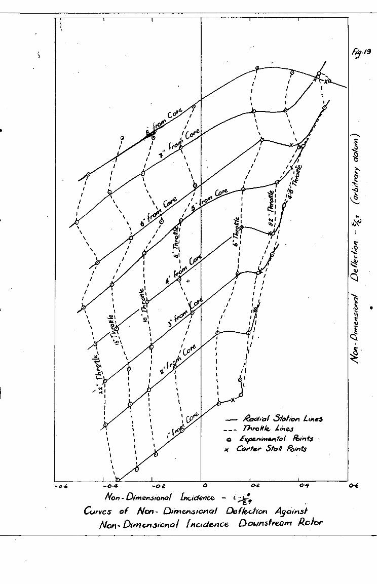
Radio( 5tation Lme5 --- Thrall& hole,' c• Evertmental lionts

Caetee Stoll 16014

-.- 0•6 -04 -42-I 0 0-2 0.4

Non-Dimensional Incidence. - cAll,

Curves. of Non- aineousional Defkchon Against

Nort- DirrionatiDno 1 inudence D ownstrearn Roior

liy.19

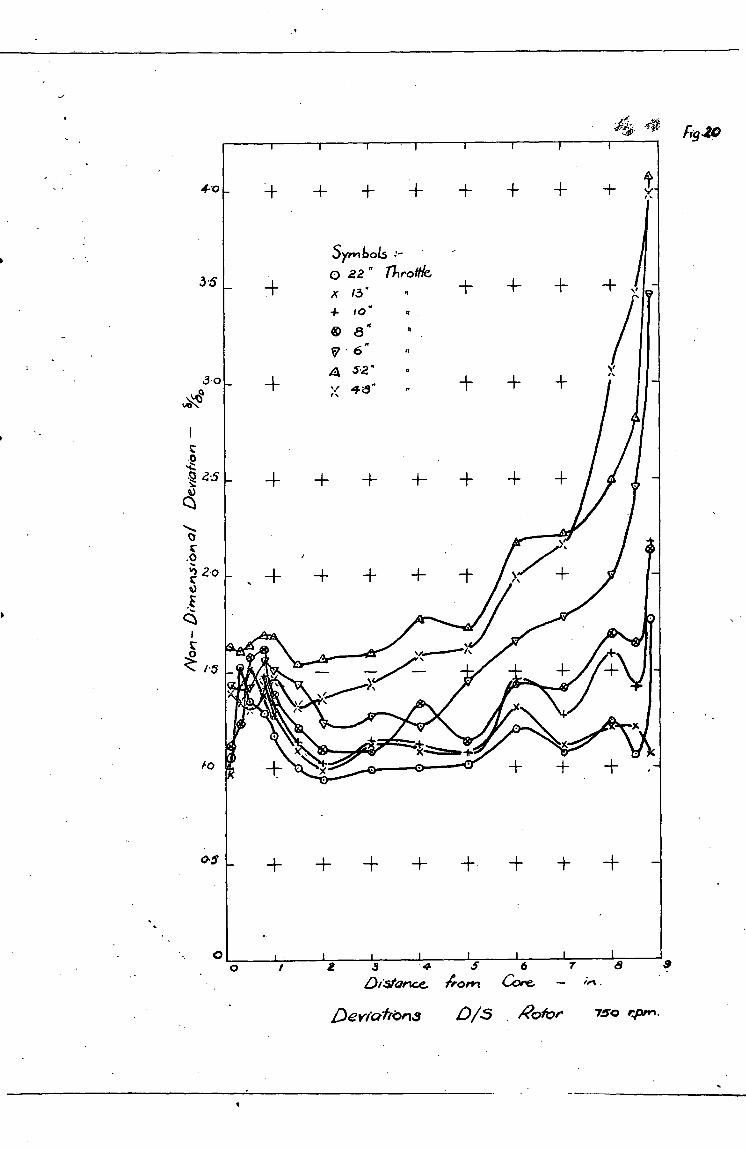
Ft9 Jo

4-0

3.5

30

4.00\1:11

Cs)

.0 ; 2o

.F

0

Fo

0 DiStarice..

S 6 7 8 9

1C0111 COM. — .

Der/a/Ions D/s Raft?" 750 rpm.

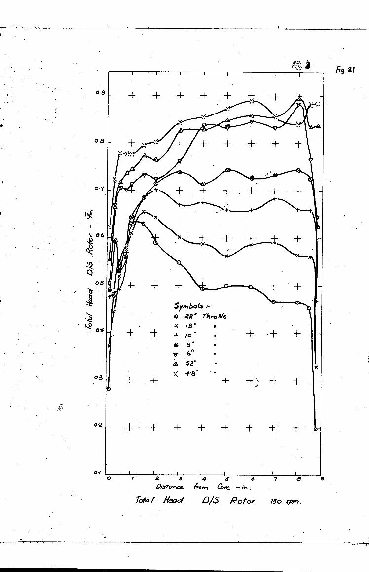
.a:stemce A,,, Co,. - .

Total Itezd D/S Rotor iso own .

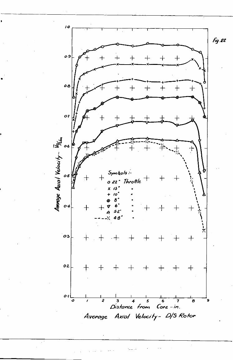
7

7

V 7

7 r a

• •

5yon op/5

O 22" rieroitie x /3"

•

+ /o ft

If

O 8' ft

+V 6" .

-- - 4.8 4

■

+ + +

+ + 9

1.0

42Z 0

0.8

0.9 + + + x x x----

+

++ ++ + ++ + -

0-2

0-I 2 3 4

a:slonce (ro.n •6 7

Cooe - 8

9

Avenage Axial Velocily- ,0/5 'co/or

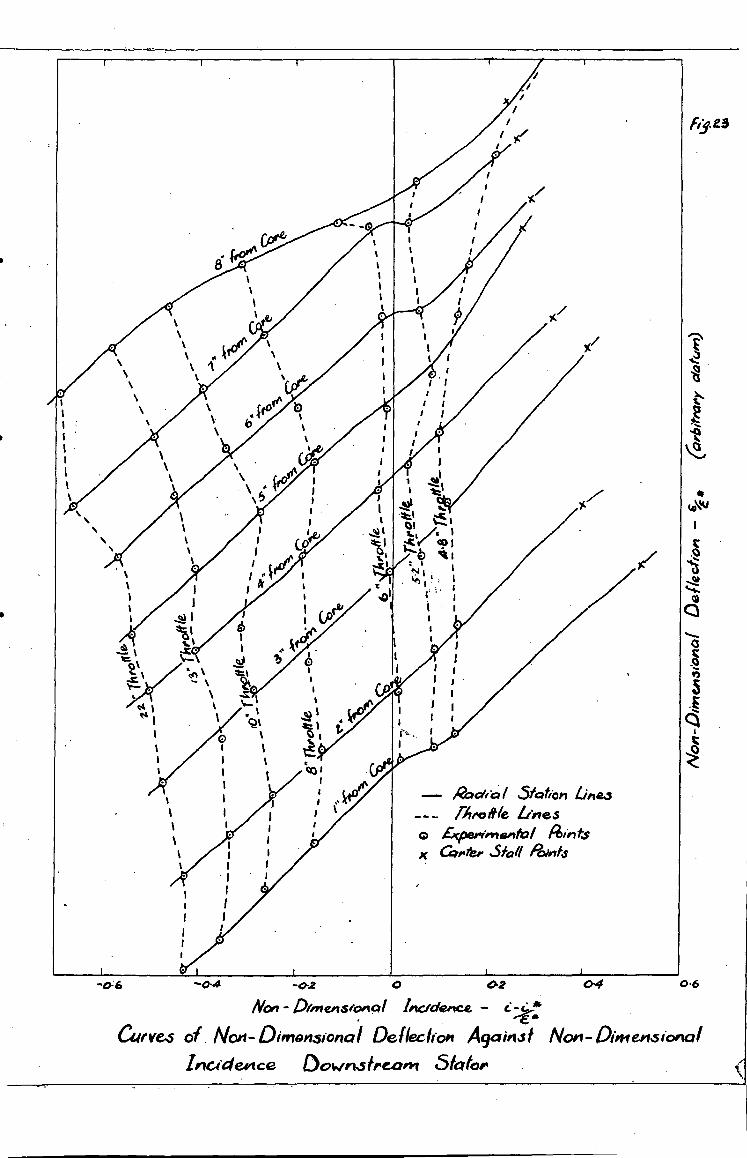
• 1

Sto

cp

Rockol Station LiPte4

Mroltle Lines o Experimental lquitts x Carter .Staff Points

1 1 1 I ,

-0-6 -0.4 -012 0 0.2 04 0.6

NO"? - Pbriensicwial Incidence -c.

Curves Of. Non-Dirnonsional Defkekon Against Non-Dimensional

Inactence Downstream 51aior

k

• ‘044)

'ZS

5

C11

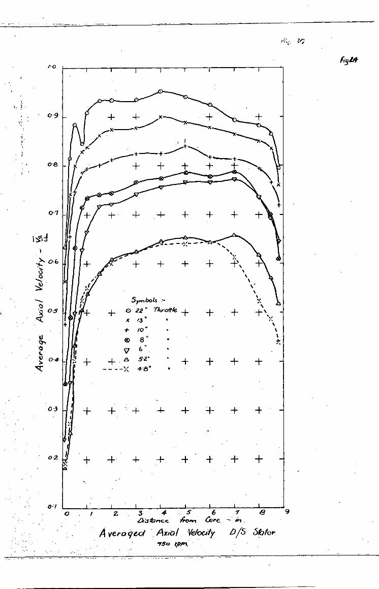
figteg-

0 3 4 .5 6 7' 8 9

..a:sbrice• Ar9.+1 &Pe 4./ .

A Vera ea APO/ Ve/OCity .0/5 (.5pior 1542 titz/n.

• ‘c.

, '

• 0.9

0 -6

0-1

--- 0 3

CZ •

0:5

ct) 0.4

0 3

0-2

0-7

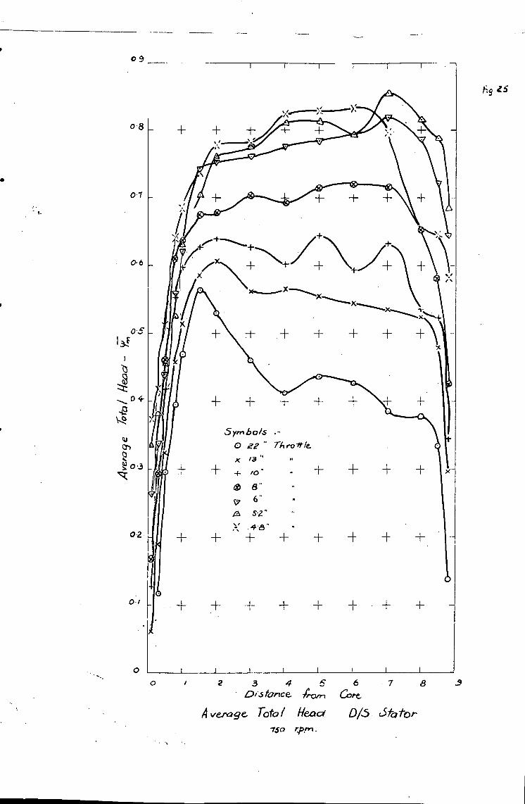
_9 8 7 6 Core

0/6 c5 fa tor

69 2 S

0 9

2 3 4 0/ Stance

Average Tot° l Head 150 'pm .

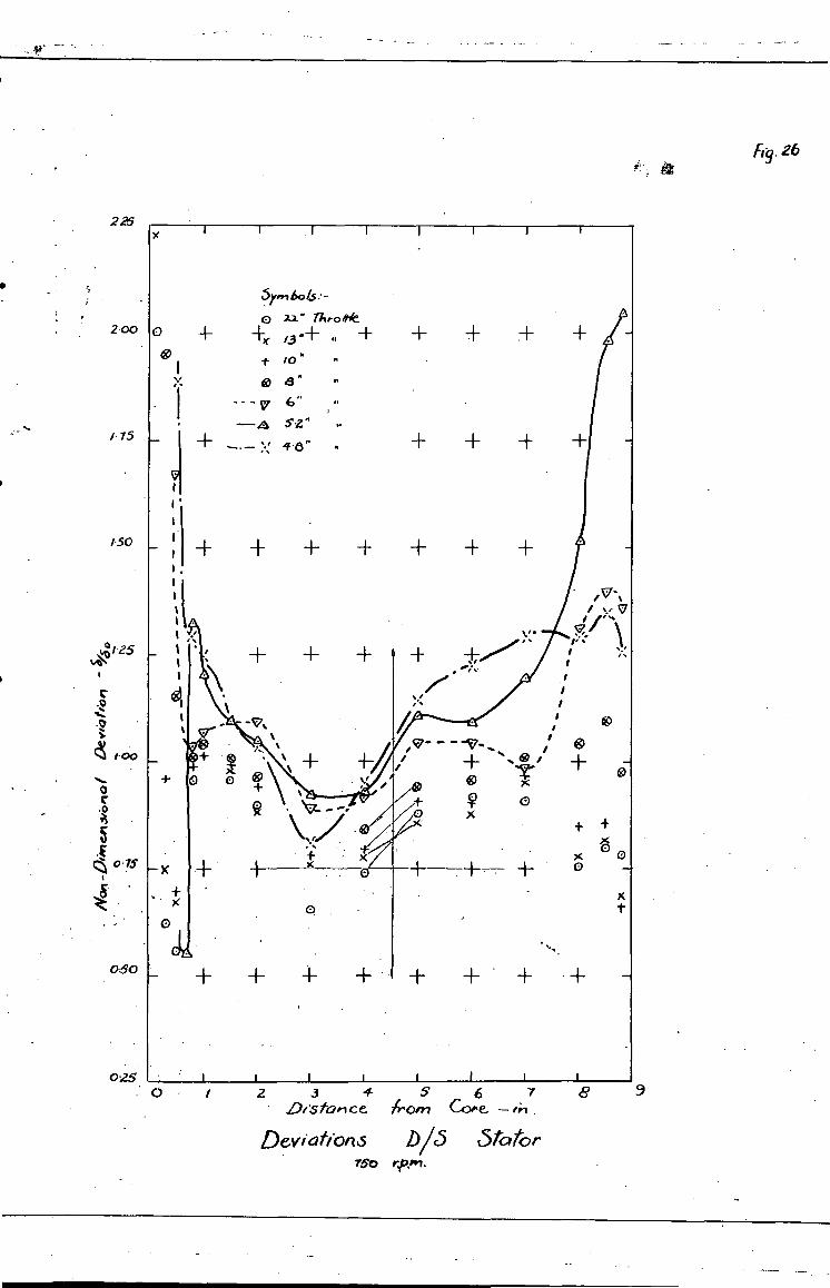
26

9 2 3 4- S 6 7

8 • D t'S /WI ce Atom Core. — .

DeViatiOrl1/45 DA5 5rOtor 750

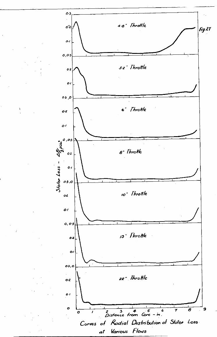
0•3

0-/

48 " PI, fiy.27.

5.2 Throttle

0 -3,0

6" rhro#/e

01

0•2

0-2

- Thro4

0

03 ,0

•••■• Ir)

02

0-f

0, 03

to - throttle

02 /3" Throttle

0-/

0-3,0

22" Throffle

J 1 I

I I I I

,Disfance Avert Coee - ;DI. 2 3 4 5 6 7 .8 t

9

Curves of Radial Dis-fri button of Stator loss

at Various Flows

02

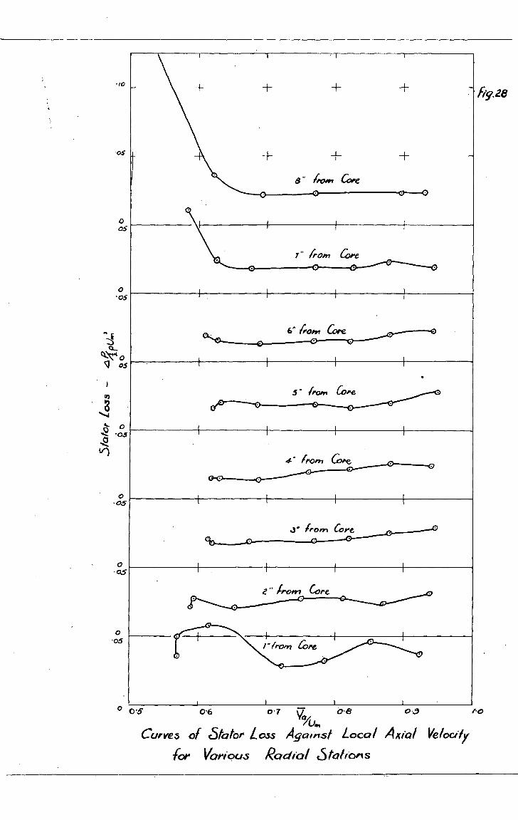
C7 c7/„., 0 .6 0 . 7

Curves of (Stator Loss Agalirst Local Axial Velocity

1or Various Radial SW foils

0 05 Po

+ + +

+ +

a- 40.“ CoPe • -0

+

+

_

_

7" from COre

•

I I

6" tisoPst COre

5" from COre

•

4- . frown am.e

..3" from CoPe

e" frOm 62re

--1

1

r(rOm GT

1 i i

•/0

05

aS

'OS

•OS

05

1.1.28

-05

0.5

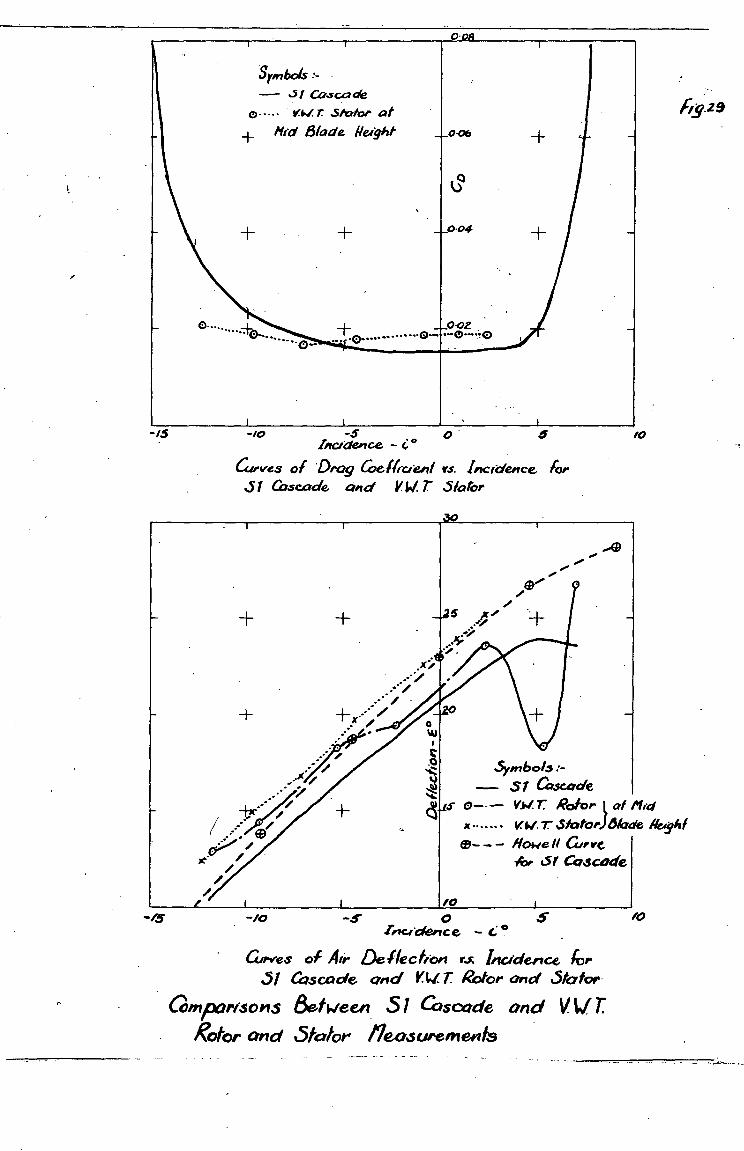
Symbo6:- — J1 Cascade

o viNir Stator ai

Hid Blade Rei01- _0-06

_•04

0 ........... ........ .0--

..••• ..•••

-1- ± .

X% 2

.1( 0

.0

*t. Spri6ols

— 57 Cascade ..." cps 0--.— vo.r Rotor at Mid

X •••••• • r Staforiakrat Ifelhf 03- - - Howe II Curve

/or 61 Cascade

/0

-10 0 0 IITClae#104 - °

Curves of Drag Coeffitient vs. Incidence for

.51 Cascade and V1•17: %Motor

-/5

429

-45 ?facie:fence

Curves of Atr Deflecfron ex Incidence kr 51 Cascade and nil: Rotor and Stator

anforisonS oefWeeit Si Cascade and vtir Rotor and Stator ne-asurements

/0

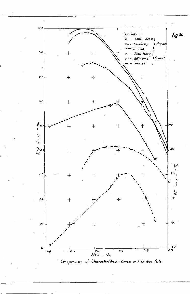
07

06 -4-

02

60 at

cl .50 0 0 7 0 8 0 9 oq 05 06

F/0., —

03

3ymbols :-

0— To/a/ Head

Effivency

— • -

Hoiie iI -- iota! Head

x - - Efficiency C.vrren

-

.

14.30 Prev,ous

04

"•••

Corn portsort Of 010,0CreriStiC,..5 6rrent and Previous Tests

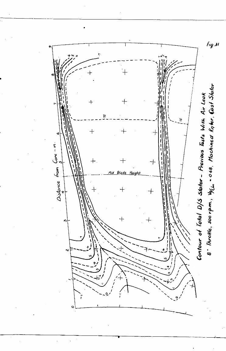
1:-

— — —

Mid

\ • \ ■ N. \ ....

S.

l 'I's .....

.

......

.5. ...

... .....,

N... 5.... ......

...... i N.

....,.

M I •/

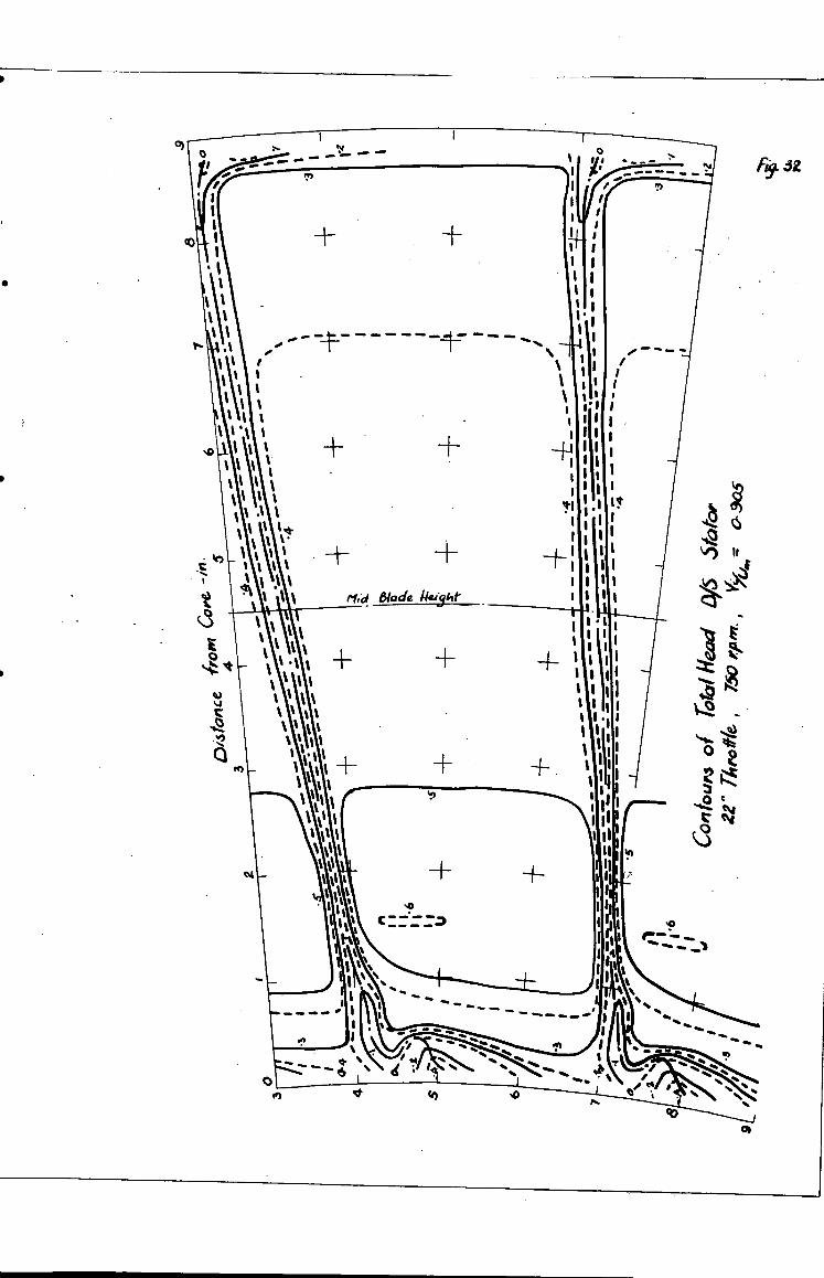
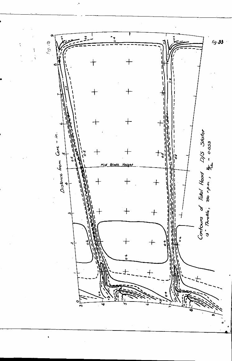
1

•

.

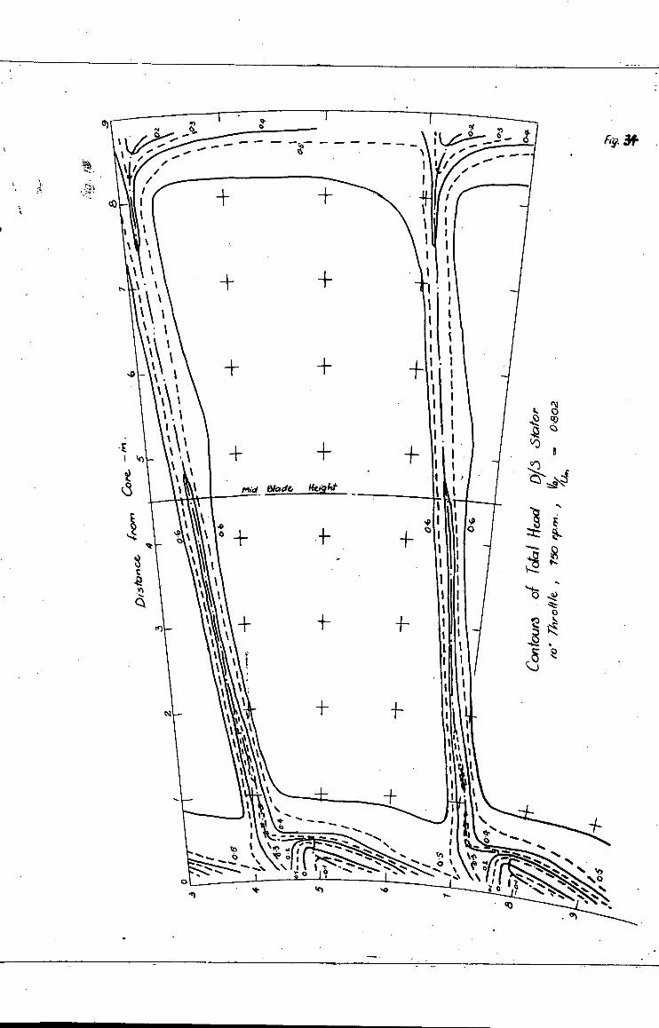
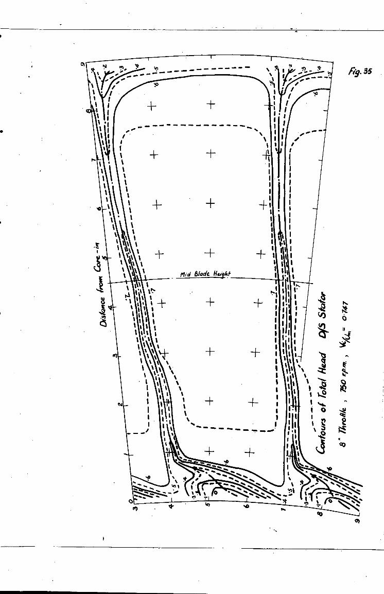
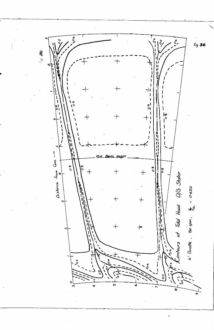
1 0

1 Mid i347616 NelYhr

--1—f

01

Ii I ' it

■••■

I.

n t%.

P \ %D ..,32 r-:... z.

\ O *,0 Ij

SCI 0 SD

/

•••• ••■• 0=. .ft•

I. I I -Iv 11

• I / I / I 1 1 /

ii Iv!

'II 1 1 I.' 1

I%

• 4.

1

'9 * .

. ....0 1 o .. v , I • •

e ..... ■ \ 0 I \ 1 ;'• \ .... .... ..‘ ,r, \ .... \ \ 1

... b \ 5% *•.." 0 ... ,r)

S. ‘ . 0 ■ ft"

F. 36

tO

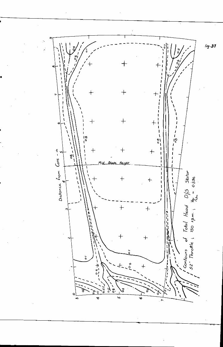
hl 31 _ tr) / o

s:O/ 0

/

I I I t I II I I

Mid blade. He ■or

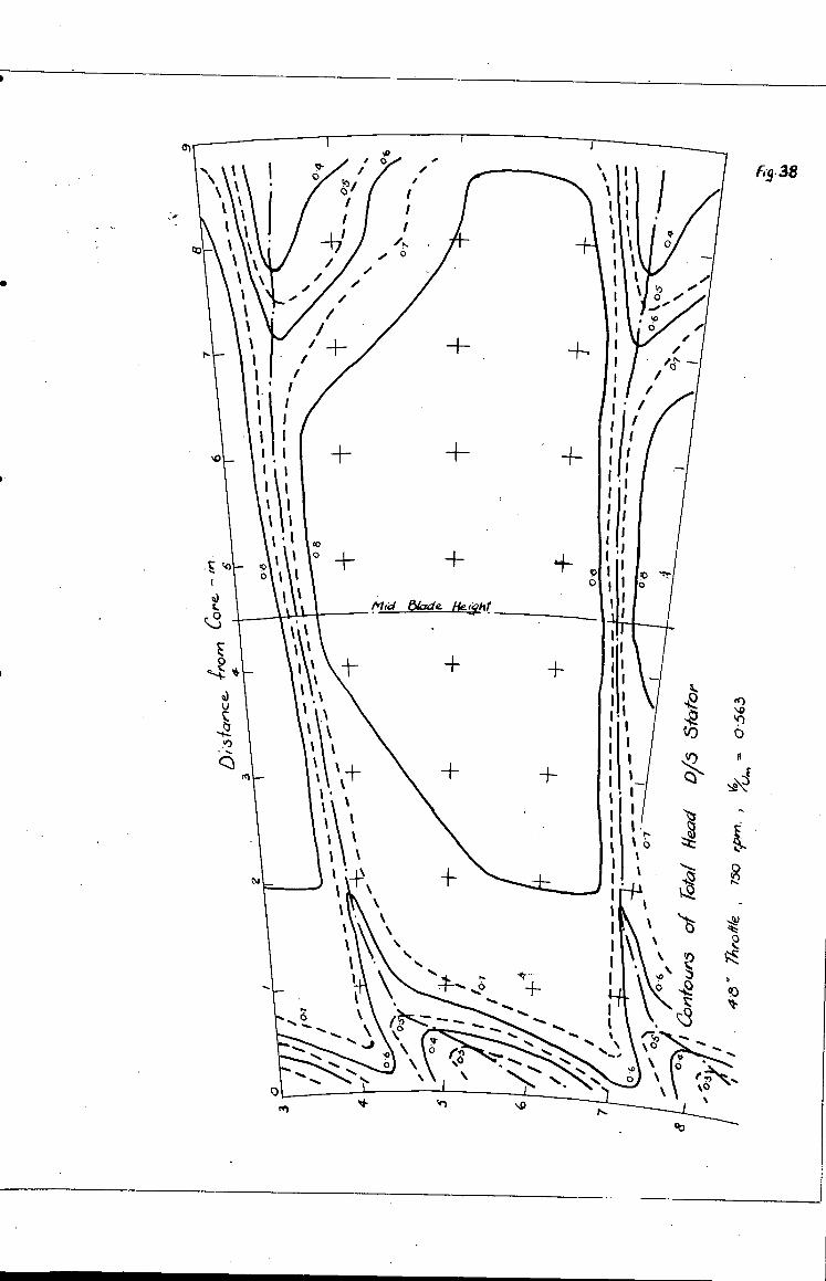
hg.38

-

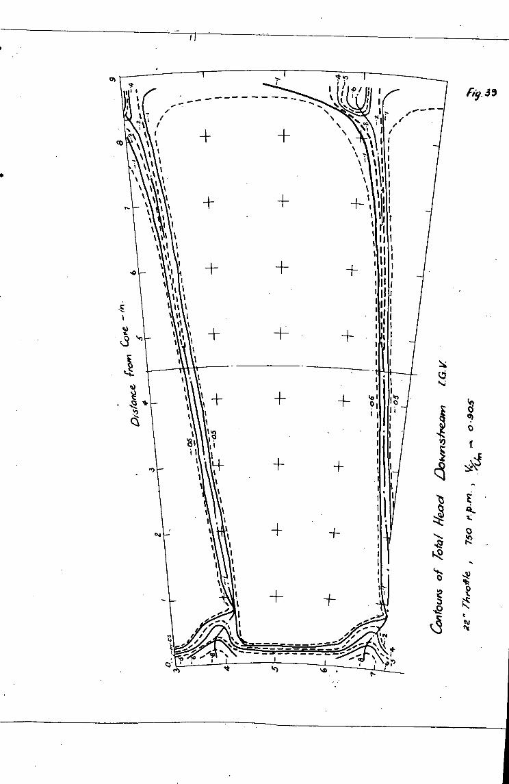
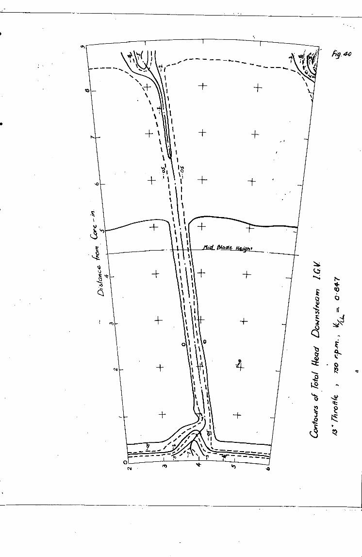
•••••• 40.

1 1 1

442

I . 1

fr)

. I o

-+

1

. 1 ' I 1

1 1

1 I

‘I • 1 1

1

+

0.. 01,2

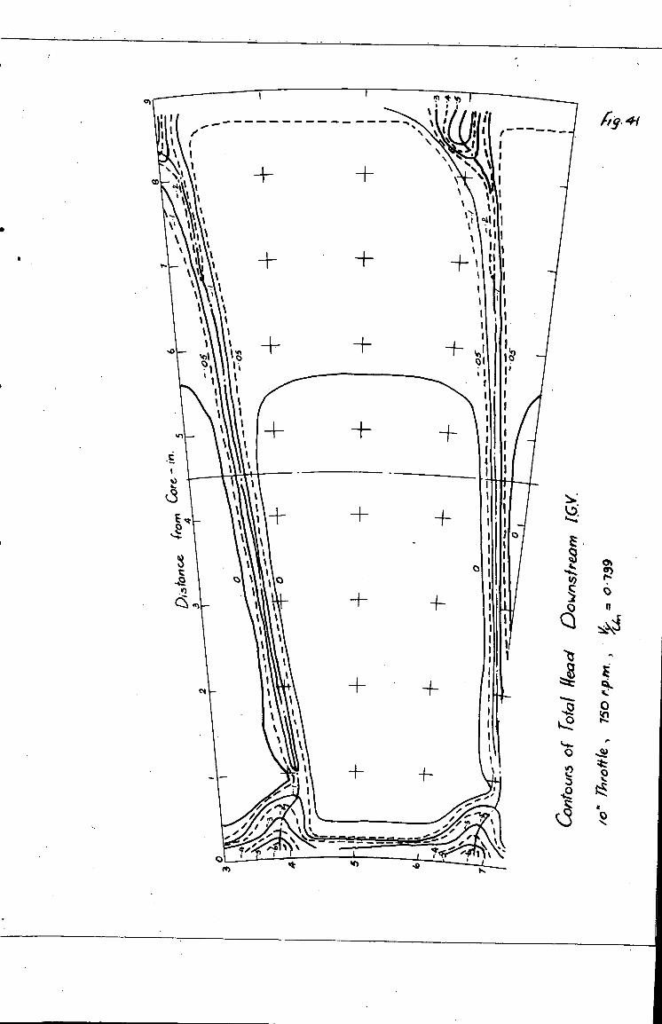
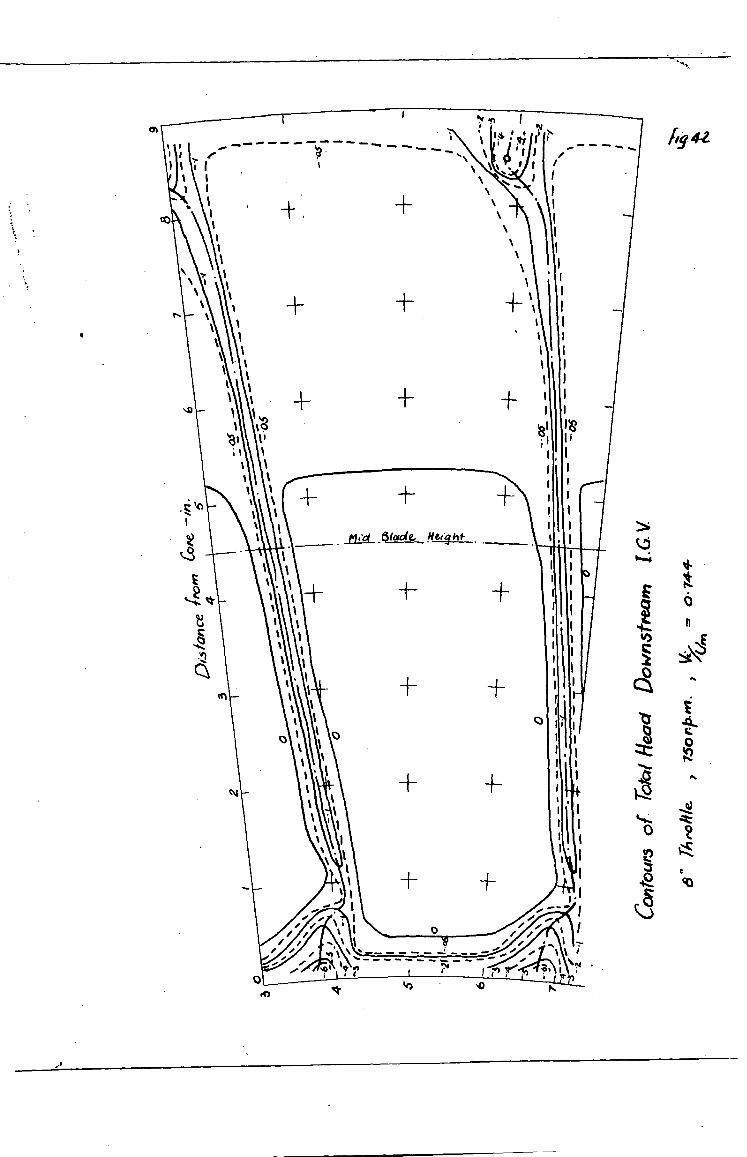
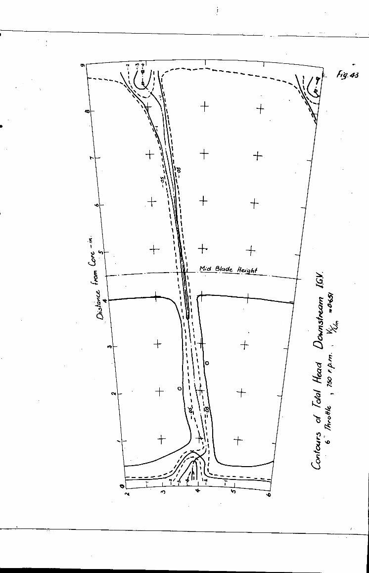
fiy. 43

...a 1 o In v) E

4

z

"4

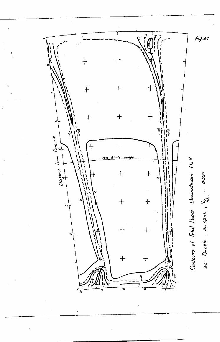
I 1

,

1

0.4

1 ' ••■••

N \ ,

11.4o

X

•

Con

tou

rs o

f ro

ta'

•

•

It

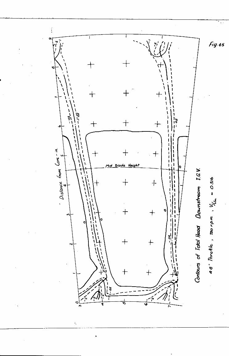
al

9 8

Fig 46

Sym bois o 22 " Thrall& K f3" rhrofile -t- /0" ThroWe

8' rhroff/e. p 6" rlirolile A 5-2" Throttle

4.8" Throtik

+ +

+ + + + + + + + ^

0-4

0.3

I I I I I I

/ 2 a 4 5 6 7 Distance (eon, Cote -

a/ryes Showing Degree of Radio/ 4a46ricirrr

4u/anal, °ohms/Peat?? Rotor

01

/.0

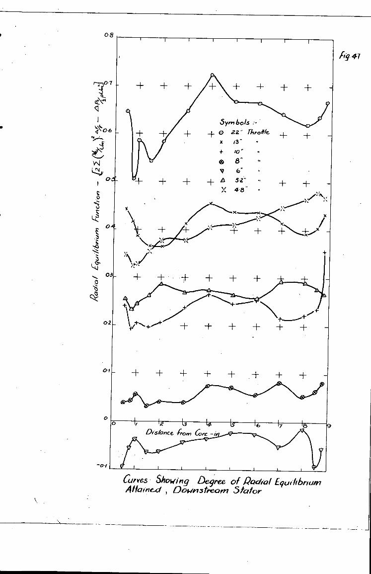
+ 22" Aro& i3"

0.1 - ± +

0-8

+ "

• 8" ✓ 6"

+

▪

± A 52 ..

X 4-8"

0-4

03_

02

+0 X

•

Curves Showing Degree of E gut hbrium Atfoine-ci Downstream Stator

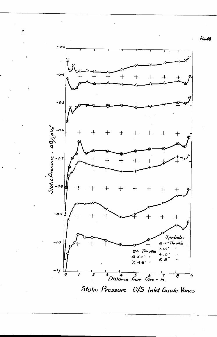
+.+ + + + + + x-- xe

x X■jicuso.0PC

0

—

••1

—o

-/-0

fi:f. 48

- 0.3

4 a

4

A

+ + + + + + + +

.7*

+ + + + + +/+

0

e.

0 o

+ + v 6" 77frolt1e

41 5.2" .1

X 48" "

Sem 6ois -

0 22" Throttle

x 13" 0

+10" VI

410 8"

1 I -1 I I I 0 1 2 3 4 5 6 7 8

Dista.,ce fro.rt Core - én .

5tatic Pressure 0/5 Inlet Guide Vanes

.9

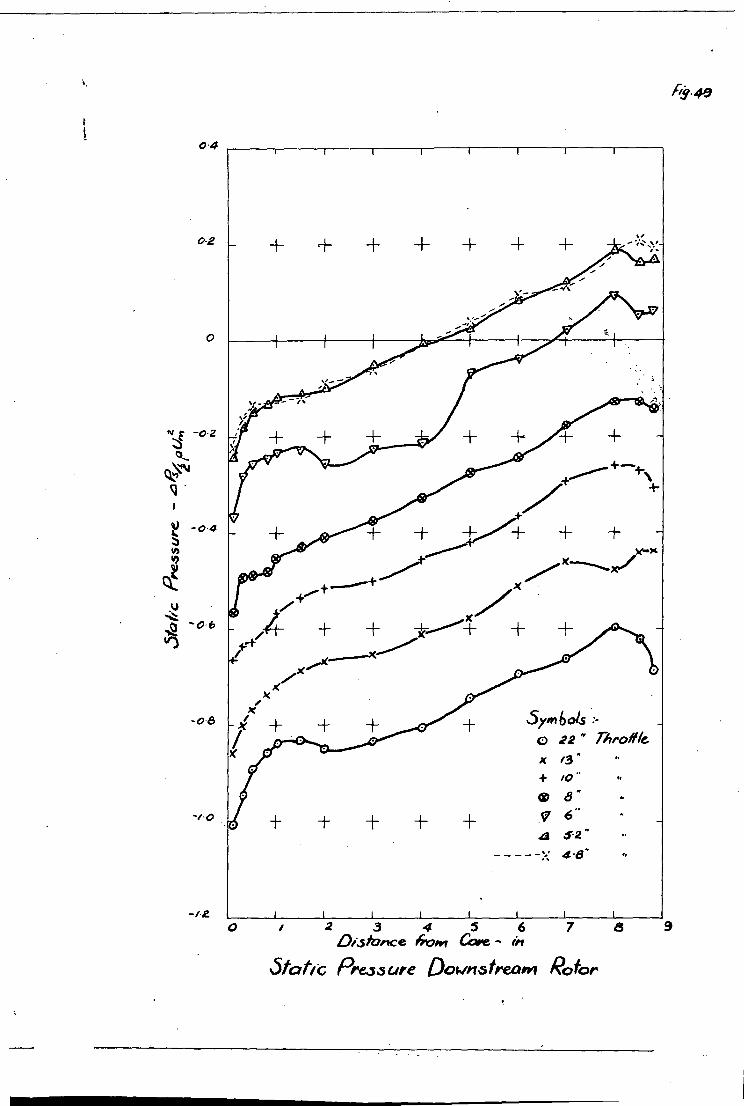
+ + -4- + 4- + o-

/ _

+4/1+ + + 51-c4C- +

/ _,1■---X-..."" 4-

V. 5r1 601S

0 22" rheOlfie

x 13 . + ,o••

CD

+ 1- +

4 52"

.5

- - - - 413 -

-0.

0 2 3 4 5 6 7 8 9 Disiance 6ufri COM rf

Static PPe35 ure DOW, stream Rotor

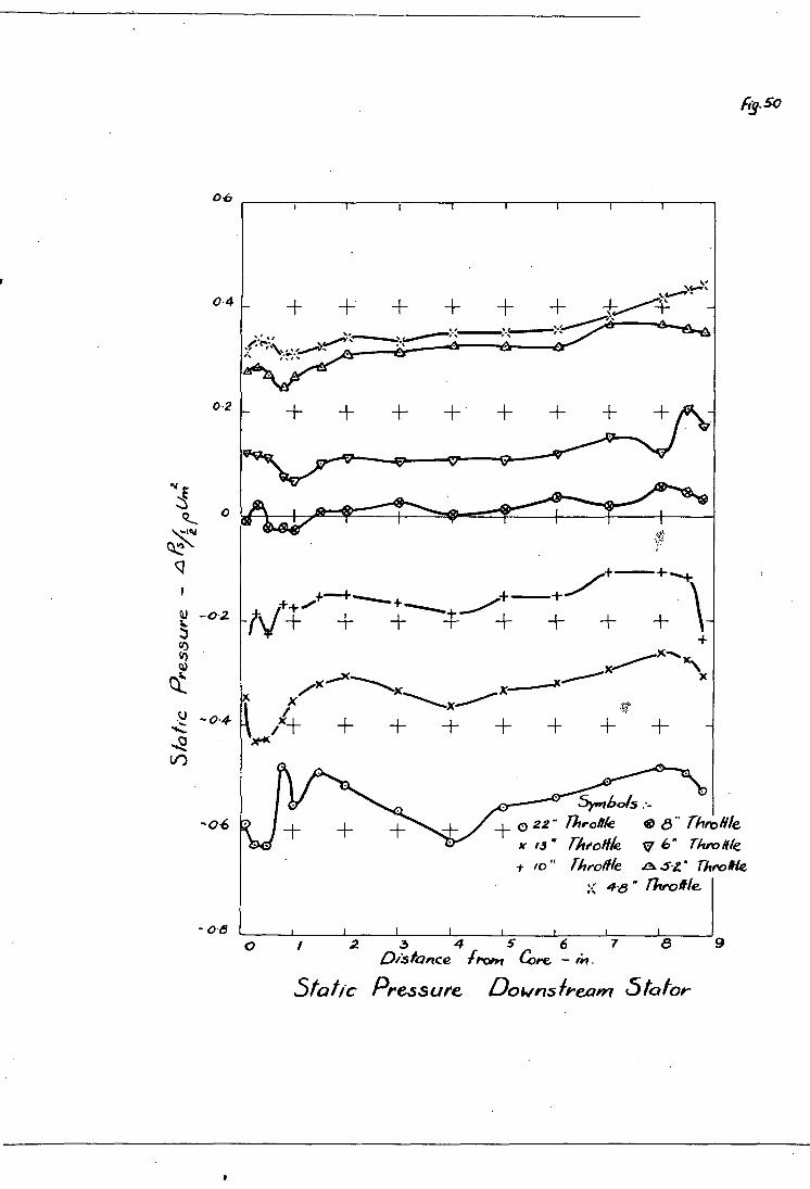
0 .6

0.4

0.2

t7L

—F- + Symbols:-

+ 0 22 - Otrodk 8" rhroHle x is" rifroftk 6" Thromle

Throttle 4,..51" Theoftle

• ;< 40" rhroille

I

U -0-2 i- --- \I + ± ± —r + + + t co

u') (t

-4.--- u —0.4. k tx

—I- /x—f— + + + + "'"----x.--•

+ + — v')‘*

- 06

I I I I 1 I I

0 1 2 3 4 5 6 Distance 'Pohl Core - 41.

Static Pressure Downstream Stator

- 0•8 7

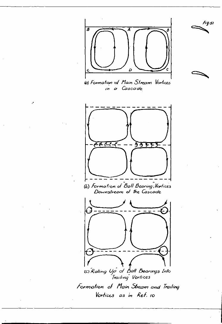
ysl c=■,

el) Formation Main Stmarn VOrkee.5 in a Cascade

(6) formation of :Boll Be,artny:Vorfices Downatrearn of the Cascade

(C);qothi-79 Un; of 3iI bearings Into

"Tn:21449" Vortices

formation of Main Skean? and 7;12/1ing

Veffices as in Ref /c7

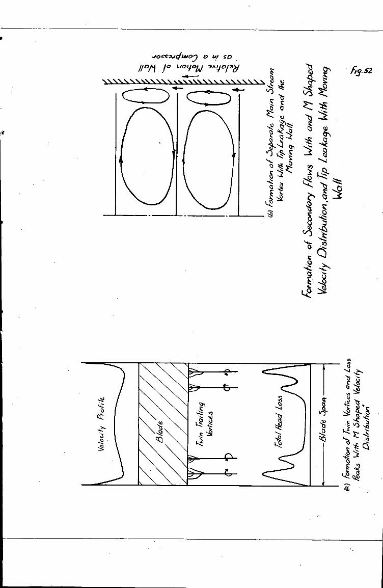
...ossaveiwoi o t., so .

Boil Jo 1.4oliou aA.yoray

-it- ■■■■■■■■‘■■■■■■■■■\■■■■■■■ \ co

-4--

To/of/

lead

&

ad

Loss

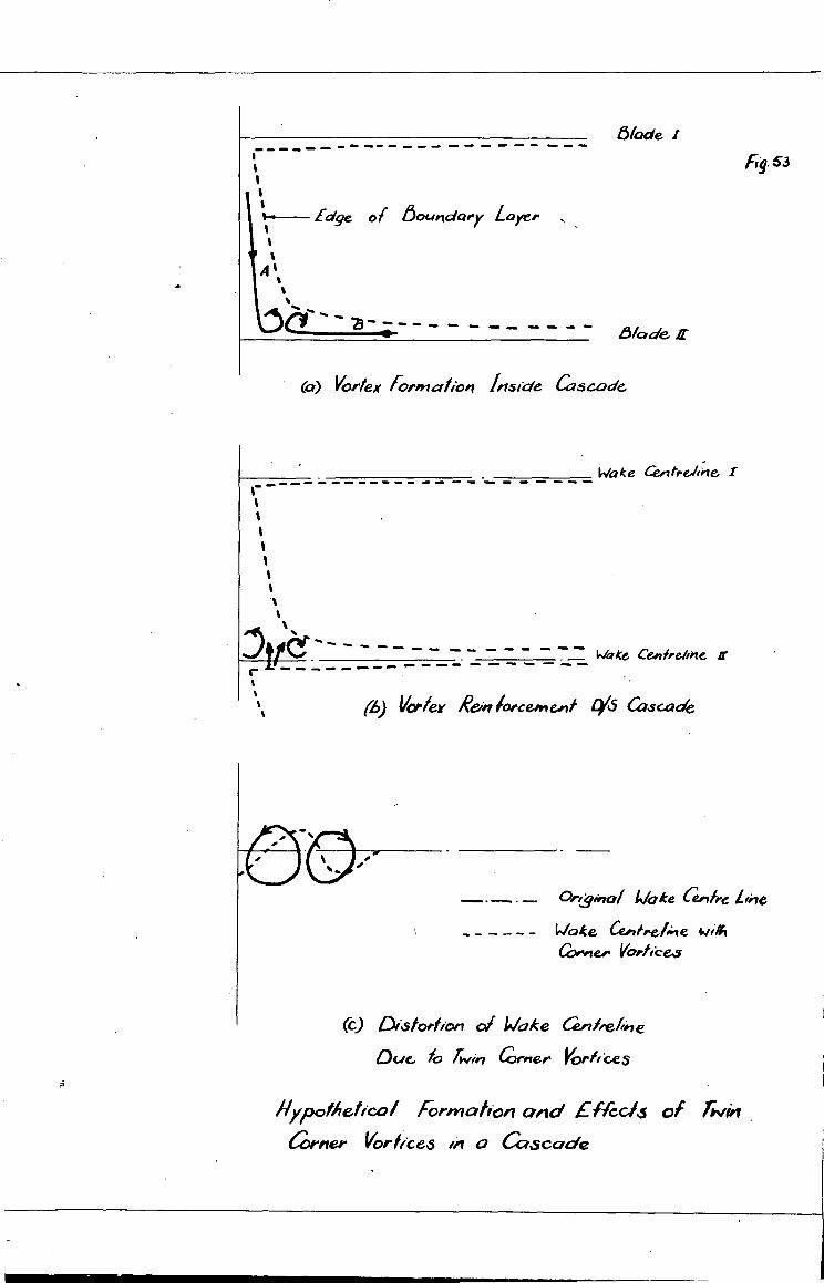
•MMID •MN. •••ID ■•• 5/onde if

•••• •MID

otode I

Edge

A l

Of 60t4riCiary Layer

(0) Vortex formation Inside Cascade

Wake Cerstre.hei" e

tpl'' ''.. ....

e■ .N.

_ __ _ ••••• almi ow. ••••■ dm. ••■• ..m. , , , Wake Cenirehote if

(b) ihrter forceine,nt 44.5 Cascade

Or(gmell Wake Cerdre brie Woke Centirebke kith; COrner

(c) Distortion of Wake Centre/41e

Due. to Twin armee Vortices

IlypotAetico/ Formaion and iffeds of Twin . alrner Vortices in o Cascade

,MINEMIM

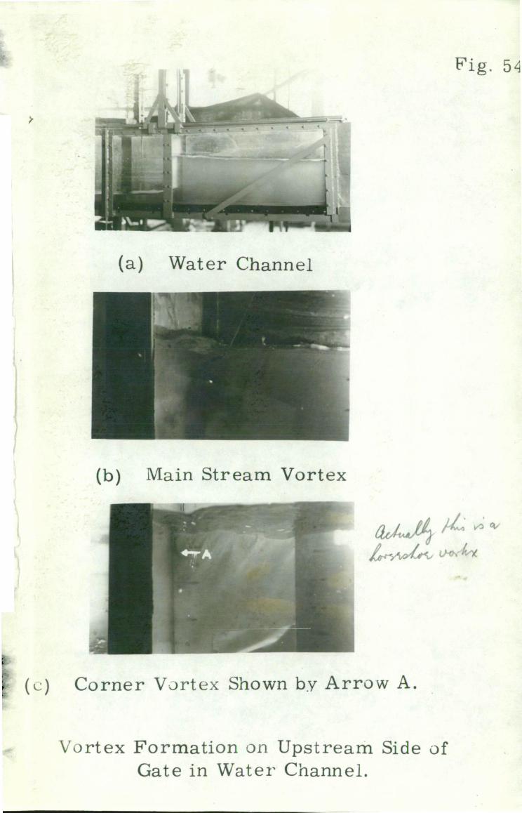
Fig. 54

a) Water Channel

(b) Main Stream Vortex

Corner VJrtex Shown by Arrow A.

Vortex Formation on Upstream Side of Gate in Water Channel.