Embed Size (px)
Citation preview

FUZZY MODELLING AND ROBUST CONTROL WITH APPLICATIONS
TO ROBOTIC MANIPULATORS
FEI ME!
B. Sc:, Nanjing University, P. R. China M. Sc., Nanjing University, P. R. China
A thesis submitted for the degree of Doctor of Philosophy at The University of Tasmania
School of Engineering Faculty of Science and Engineering
The University of Tasmania Hobart, Tasmania 7001
Australia
December, 1999

Authority of Access
This thesis may be made available for loan. Copying of any part of this thesis is
prohibited for two years from the date this statement was signed; after that time
limited copying is permitted in accordance with the Copyright Act 1968.

Statement of Originality
The work contained in this PhD thesis is original, to the best of my knowledge and
belief, except as acknowledged in the text. This thesis contains no material which has
been accepted for the award of any other degree or diploma in any tertiary institution.
Fei Mei
Ii

Acknowledgements
I wish to thank the many people who have helped me complete this thesis. For
encouragement and support, I would especially like to thank my supervisor and friend,
Dr. Man Zhihong. His enthusiasm and motivation has helped me greatly. I am
particularly grateful to Prof. Thong Nguyen, my co-supervisor, for his valuable advice
and consistent encouragement during my work. My grateful thanks also go to all the
members and postgraduates in the School of Engineering for their kind reception and
cooperation that I found during my PhD candidature at The University of Tasmania.
For financial support, I am grateful to The University of Tasmania for providing me
with Tasmania International Scholarships. Finally, I would like to thank my wife Bing
Xu, my daughter, Lisa Jun Mei, my parents and my friends for their love,
understanding and support during this period.

Abstract
In this thesis, fuzzy modelling of a class of nonlinear systems has been investigated
based on fuzzy logic and linear feedback control theory, and a few robust variable
structure control schemes for nonlinear systems have been developed. A number of
robustness and convergence results with dramatically reduced control chattering are
presented for variable structure control systems with applications to robotic
manipulators in the presence of parameter variations and external disturbances. The
major outcomes of the work described in this thesis are summarised as follows.
A robust tracking control scheme is proposed for a class of nonlinear systems with
fuzzy model. It is shown that a nominal system model for a nonlinear system is
established by fuzzy synthesis of a set of linearised local subsystems, where the
conventional linear feedback control technique is used to design a feedback controller
for the fuzzy nominal system. A variable structure compensator is then designed to
eliminate the effects of the approximation error and system uncertainties. Strong
robustness with respect to large system uncertainties and asymptotic convergence of
the output tracking error are obtained.
A sliding mode control scheme using fuzzy logic and Lyapunov stability theory has
been proposed. It is shown that a sliding mode is first designed to describe the desired
system dynamics for the controlled system. A set of fuzzy rules are then used to adjust
the controller's parameters based on the Lyapunov function and its time derivative.
The desired system dynamics are then obtained in the sliding mode. The sliding mode
controllers with fuzzy tuning algorithm show the advantage of reducing the chattering
of the control signals, compared with the conventional sliding mode controllers.
A robust continuous sliding mode control scheme for linear systems with uncertainties
has been presented. The controller consists of three components: equivalent control,
continuous reaching mode control and robust control. It retains the positive properties
of sliding mode control but without the disadvantage of control chattering. The
iv

proposed control scheme has been applied to the tracking control of a one-link robotic
manipulator with fuzzy modelling of the nonlinear system.
A robust adaptive sliding mode control scheme with fuzzy tuning has been presented.
It is shown that an adaptive sliding mode control is first designed to learn the system
parameters with bounded system uncertainties and external disturbances. A set of
fuzzy rules are then used to adjust the controller's uncertainty bound based on the
Lyapunov function and its time derivative. The robust adaptive sliding mode
controller with fuzzy tuning algorithm show the advantage of reducing the chattering
and the amplitude of the control signals, compared with the adaptive sliding mode
controller without fuzzy tuning. Experimental example for a five-bar robot arm is
given in support of the proposed control scheme.
Finally, a new adaptive sliding mode controller has been developed for trajectory
tracking in robotic manipulators. This controller is able to estimate the constant part
of the system parameters as well as adaptively learn the uncertain part of the system
parameters by the Gaussian neural network. It is shown that under a mild assumption,
the proposed control law does not require measurement of acceleration signals. This
new control law exhibits the good aspects of Slotine and Li's (1987) and keeps the
chattering to a minimum level. An experiment of a five bar robotic system was done
and the results have confirmed the effectiveness of the approach.
List of Publications
1. Fei Mei, Man Zhihong, Yu Xinghuo, Thong Nguyen, "A Robust Tracking
Control Scheme for a Class of Nonlinear Systems with Fuzzy Nominal
Model", International Journal of Applied Mathematics and Computer Science, vol.8, No.1, pp.145-158, 1998.
2. Fei Mei, Man Zhihong, Thong Nguyen, "Fuzzy Modelling and Tracking
Control of Robotic Manipulators", to appear in Mathematical and Computer
Modelling, 1999.
3. Fei Mei, Man Zhihong, Xinghuo Yu, "Robust adaptive sliding mode control of
robots", submitted to IEEE Transactions on Industrial Electronics, 1999.
4. Xinghuo Yu, Man Zhihong, S S Cong, Fei Mei, "Robust adaptive sliding mode
control of robotic manipulators", International Journal of Robotics and
Automation, vol.14, no.2, pp. 54-60, 1999.
5. Fei Mei, Man Zhihong, "A Sliding Mode Control System with Fuzzy Logic
Controller", International Conference on Computational Intelligence and
Multimedia Applications, 9-11 February, 1998, Monash University, Australia.
6. Fei Mei, Man Zhihong, "Fuzzy Modelling and Tracking Control of Nonlinear
Systems", International Congress on Modelling and Simulation Proceedings,
pp. 902-906, 7-12 December, 1997, Hobart, Australia.
7. Fei Mei, Man Zhihong, Thong Nguyen, "Continuous sliding mode control with
limited control input", Proceedings of the Australian Universities Power
Engineering Conference (AUPEC'98), Hobart, Australia, vol.1, pp212-216,
September, 1998.
8. Fei Mei, Man Zhihong, Thong Nguyen, "The terminal controller design with
application to robotic manipulators", Proceedings of the Australian
Universities Power Engineering Conference (AUPEC'98), Hobart, Australia,
vol.2, pp532-536, September, 1998.
9. Fei Mei, Michael Negnevitsky, "A robust continuous sliding mode control
scheme", Proceedings of 6" International Conference on Fuzzy Theory and Technology, Durham, USA, vol.', pp292-294, October 23-28, 1998.
vi

10. Fei Mei, "Sliding mode control signal analysis by discrete wavelet transform",
Proceedings of the .14 th World Congress of International Federation of
Automatic Control (IFAC'99), Beijing, China, vol. H, pp. 349-353, July 5-9,
1999.
11. Man Zhihong, Fei Mei, "A sliding mode control for nonlinear SISO
systems with a new fuzzy model", Proceedings of the 14" World Congress
of International Federation of Automatic Control (IFAC99), Beijing, China,
vol. Q, pp. 359-362, July 5-9, 1999.
12. Fei Mei, Man Zhihong, Xinghuo Yu, Wei Lai, "RBF network based sliding
mode control of robots", Proceedings of the IEEE Hong Kong Symposium on
Robotics and Control, Hong Kong, vol. 1, pp.27-32, July 2-3, 1999.
vii

TABLE OF CONTENTS viii
Contents
Statement of Originality ii
Acknowledgements iii
Abstract iv
List of Publications vi
1 Introduction 1
1.1 MOTIVATION 1
1.2 SCOPE 4
1.3 THESIS OUTLINE 5
2 A survey of variable structure control theory .9
2.1 INTRODUCTION 9
2.2 BASIC VARIABLE STRUCTURE CONTROL THEORY 11
2.2.1 SYSTEM MODEL AND SLIDING MODE 11
2.2.2 EQUIVALENT CONTROL 13
2.2.3 ROBUSTNESS PROPERTY 16
2.2.4 Two METHODS OF SLIDING MODE DESIGN 17
2.2.5 CONTROLLER DESIGNS 21
2.3 VARIABLE STRUCTURE CONTROL OF NONLINEAR SYSTEM 22
2.3.1 SYSTEM MODEL 22
2.3.2 SLIDING MODE AND EQUIVALENT CONTROL 23
2.3.3 CONTROLLER DESIGN 24
2.3.3.1 Diagonalisation method 24

TABLE OF CONTENTS ix
2.3.3.2 Reaching law method 25
2.3.4 ROBUST CONTROL OF NONLINEAR SYSTEMS 27
2.4 APPLICATION TO ROBOT MANIPULATORS 29
2.4.1 DYNAMICS OF ROBOTIC MANIPULATORS 29
2.4.2 A ROBUST VSC CONTROLLER DESIGN 31
2.5 CONCLUDING REMARKS 33
3 Fuzzy logic and fuzzy logic controller 35
3.1 INTRODUCTION 35
3.2 FUZZY SET THEORY 37
3.2.1 FUZZY SETS 38
3.2.2 SET THEORETICAL OPERATORS 40
3.2.3 THE EXTENSION PRINCIPLE 42
3.2.4 FUZZY RELATIONS AND THEIR COMPOSITIONS 43
3.2.5 LINGUISTIC REPRESENTATION 45
3.3 FUZZY LOGIC AND FUZZY REASONING 48
3.4 FUZZY LOGIC CONTROL 54
3.5 CONCLUDING REMARKS 68
4 Fuzzy modelling and robust tracking control of nonlinear systems 70
4.1 INTRODUCTION 70
4.2 LINEARISATION OF NONLINEAR SYSTEMS 72
4.3 FUZZY MODELLING AND TRACKING CONTROL OF NONLINEAR SYSTEMS 74
4.3.1 FUZZY MODELLING AND TRACKING CONTROLLER DESIGN 74
4.3.2 A SIMULATION EXAMPLE 76
4.4 ROBUST TRACKING CONTROL WITH FUZZY NOMINAL MODEL 86
4.4.1 A ROBUST TRACKING CONTROL SCHEME 86

TABLE OF CONTENTS x
4.4.2 A SIMULATION EXAMPLE 90
4.5 CONCLUDING REMARKS 93
5 Fuzzy sliding mode control .98
5.1 INTRODUCTION 98
5.2 SLIDING MODE CONTROL OF NONLINEAR SYSTEMS 99
5.3 FUZZY TUNING OF THE SLIDING MODE CONTROLLER 101
5.4 AN ILLUSTRATIVE EXAMPLE 106
5.5 CONCLUDING REMARKS 111
6 Robust continuous sliding mode control .112
6.1 INTRODUCTION 112
6.2 A ROBUST CONTINUOUS SLIDING MODE CONTROL 114
6.3 A SIMULATION EXAMPLE 117
6.4 CONCLUDING REMARKS 120
7 Fuzzy adaptive sliding mode control . 132
7.1 INTRODUCTION 132
7.2 ROBUST ADAPTIVE SMC WITH FUZZY TUNING 134
7.3 AN ILLUSTRATIVE EXAMPLE 142
7.4 CONCLUDING REMARKS 145
8 Robust adaptive sliding mode control of robots .153
8.1 INTRODUCTION 153
8.2 THE ROBUST ADAPTIVE SMC DESIGN 155
8.3 EXPERIMENTAL RESULTS 163
8.4 CONCLUDING REMARKS 167

TABLE OF CONTENTS xi
9 Conclusions 172
9.1 SUMMARY 172
9.2 SUGGESTIONS FOR FUTHER WORK 175
References .177
Appendix 194
A HARDWARE SETUP FOR A FIVE-BAR ROBOT ARM 194
B C++ PROGRAMS FOR A FUZZY SLIDING MODE CONTROLLER 198 ,
FSMC.CPP 198
FSMC DATA . TXT 208
FSMC DATA.H 209
COMPLEX.CPP 212
CONTAINER.CPP 218
LEAST SQUARES.CPP 222
MISC.CPP 230
MY_MATH.CPP 231
MY_PROCESS.CPP 244
PATH.CPP 248
PC30 GwEIO.CPP 250
PCL833.CPP 254
RUNGA KUTTA 4 111 ORDER.CPP 258
VECTOR.CPP 260

CHAPTER I INTRODUCTION 1
Chapter 1
Introduction
1.1 Motivation
The basis for control system design and stability analysis is a dynamic mathematical
model that captures prominent features of the system under consideration. However,
in practical situations, such a requirement is not feasible because the controlled
systems have high nonlinearities and uncertain dynamics, and simple linear or
nonlinear differential equations cannot sufficiently represent the corresponding
practical systems, and therefore, the designed controller based on such a model cannot
guarantee the good performance such as stability and robustness.
During the last few years, fuzzy logic control has been suggested as an alternative to
conventional control techniques for complex nonlinear systems due to the fact that
fuzzy logic combines human heuristic reasoning and expert experience to approximate
a certain desired behaviour function (Takagi and Sugeno, 1985; Cao et al., 1996;
Wang et al., 1996). However, the asymptotic error convergence and stability of the
closed-loop system may not be obtained due to the approximation error and
uncertainties of the fuzzy model.

CHAPTER 1 INTRODUCTION 2
Many kinds of fuzzy models for control processes have been developed since
Mamdani's (1974) paper was published. They can be classified into three kinds of
models, Composition Rule of Inference (Zaheh, 1973), Approximate Reasoning
Model (Nakanishi et al., 1993), Sugeno's Models such as Position type Model and
Position-Gradient type Model (Sugeno and Yasukawa, 1993). Most of these models
are expressed by a set of fuzzy linguistic propositions which are derived from the
experience of skilled operators or by fuzzy implication which locally represent linear
input-output relations of the system.
Most proposed conventional fuzzy models only consider the external behaviour of the
system, and can be considered as a function approximation. It is very difficult to
obtain a controller using those models. Even if the controller can be obtained by using
some trial-and-error procedures the behaviour of the closed-loop system, for example,
the stability of the system is still difficult to analyse. Also the number of rules increase
very quickly when the system becomes complex because every local rule is only
described by a constant. Therefore, the identification of these fuzzy models is still a
difficult problem because there are too many parameters in the membership functions.
From a control point of view, system uncertainties can be classified as either
structured or unstructured. Structured uncertainties are those dynamics that have a
known functional form but unknown parameters, while unstructured uncertainties are
simply those that are not structured. For example, system parameters and payload for a
robotic system can be viewed as structured uncertainties; unstructured uncertainties
include friction, disturbances, and unmodelled dynamics.

CHAPTER 1 INTRODUCTION 3
Two major conventional control methodologies have been developed for dealing with
system uncertainties: adaptive control and robust control. Adaptive control is a
control scheme in which so-called adaptation laws are constructed to learn explicitly
unknown constant parameters of the system under control. For this reason, adaptive
control is limited to those systems whose uncertainties are structured, although it is
applicable to a wider range of uncertainties after employing robustness enhancement
techniques. Robust control is a control of fixed structure that guarantees stability and
performance for uncertain systems. Its design only requires some knowledge about
bounding functions on the greatest possible value of the uncertainties. This implies
that robust control is capable of compensating for both structured and unstructured
uncertainties.
Variable structure control with sliding mode is a robust control technique with respect
to system variations and external disturbances. Variable structure control was
pioneered in the former Soviet Union in the 1960s by Emelyanov (1962, 1966) and
then developed by many researchers (Uticin, 1971, 1977, 1978, 1983; Itks, 1976;
Young, 1978, 1988; Slotine and Sastry, 1983; Gao and Hung , 1993). However, the
control technique has not been widely accepted in the practical control engineering
community, due mainly to the worry of chattering which is inherent in the variable
structure control system.
This introduces the possibility of using conventional variable structure control method,
and fuzzy logic technique to develop better control schemes for complex systems. In
other words, "can fuzzy logic (with its powerful capabilities for modelling and control

CHAPTER 1 INTRODUCTION 4
of complex systems) and conventional linear or nonlinear control theory be combined
to improve the system performance and control quality?". The aim of this thesis is to
show that by considering both these areas, superior system performance and control
quality can be achieved.
1.2 Scope
The aim of this thesis is to present new robust control schemes by incorporating
artificial intelligent techniques such as fuzzy logic and neural networks with
conventional variable structure control system. In line with this, a review of basic
variable structure control theory and discussion of recent research results on the robust
variable structure control for a class of nonlinear systems with uncertain dynamics is
given.
Fuzzy logic and fuzzy logic control are also reviewed to present a background to the
methodology to be employed. Fuzzy sets, fuzzy reasoning, and fuzzy controller design
are described.
The body of the thesis is devoted to fuzzy modelling of a class of nonlinear systems
and developing robust variable structure control schemes by employing fuzzy logic,
neural networks and adaptive control techniques. The rationale is explained more fully
at the end of Chapter 2 and 3, followed by the robust control scheme development in
the succeeding chapters. A review of the contents of the thesis is given in Section 1.3.

CHAPTER 1 INTRODUCTION 5
1.3 Thesis outline
The thesis is organised as follows.
In Chapter 1, the major thrust of the thesis, the motivation, scope and thesis outline are
introduced.
In Chapter 2, the basic theory of variable structure control systems is briefly surveyed.
Because the variable structure theory has many good features, it can be easily used to
design controllers for linear or nonlinear systems. Although the robustness can be
achieved without the exact knowledge of the control system, the system performance
and control quality depend very much on the choosing of sliding mode parameters and
the estimating of bounding functions of the system's unknown parts. In practice,
excessive control input and severe control chattering which may excite unmodelled
high-frequency dynamics are highly undesirable. In the following chapters of this
thesis, several new and improved robust variable structure control schemes of
nonlinear systems will be proposed by combining conventional methods and recently
developed techniques, namely fuzzy logic and neural networks, and it will be shown to
improve the system performance and enhance the control quality.
Chapter 3 provides a background of fuzzy logic and fuzzy logic control techniques to
be applied in the later chapters. Fuzzy sets, fuzzy set operations, and fuzzy linguistic
representation such as linguistic variables and linguistic modifiers (hedged) will be
briefly outlined. Fuzzy reasoning or approximate reasoning is considered from the
engineering viewpoint with IF-THEN fuzzy implications using Mamdani's minimum
inference and Larsen's product inference. A fuzzy logic controller, mapping an input
data vector into a scalar control output, normally comprises a rule base, fuzzifier and

CHAPTER 1 INTRODUCTION 6
defuzzifier. Commonly-used kinds of membership functions are described, focusing
on control applications. The prominent advantage of the fuzzy logic controller is that
it can effectively control complex ill-defined systems having nonlinearities, parameter
variations and disturbances. However, there also exist some impediments in the
design of the fuzzy logic controller. In general, fuzzy rules are obtained on the basis
of intuition and experience, and membership functions are selected by trial and error
procedure. Moreover, it is not easy to mathematically prove the system stability and
robustness due to linguistic expression of the fuzzy rules. Therefore, a systematic
design method of the fuzzy logic controller from which the stability and robustness
can be clearly seen is to be explored (Lee, 1990). The succeeding chapters will employ
fuzzy logic to establish system model of a class of nonlinear systems and enhance
robustness and control quality of variable structure control systems.
In Chapter 4, a robust tracking control scheme is proposed for a class of nonlinear
systems. The main contribution of this scheme is that a nominal system model for a
nonlinear system is established by fuzzy synthesis of a set of linearised local
subsystems, where the conventional linear feedback control technique is used to
design a feedback controller for the fuzzy nominal system. A variable structure
compensator is then designed to eliminate the effects of the approximation error and
system uncertainties. Strong robustness with respect to large system uncertainties and
asymptotic convergence of the output tracking error are obtained. A simulation
example is given to support the proposed control scheme.
In Chapter 5, Lyapunov stability theory and fuzzy logic technique are combined
together to design sliding mode control systems. It is shown that a sliding mode is

CHAPTER I INTRODUCTION 7
first designed to describe the desired system dynamics for the controlled system. A set
of fuzzy rules are then used to adjust the controller's parameters based on the
Lyapunov function and its time derivative. The desired system dynamics are then
obtained in the sliding mode. The sliding mode controllers with fuzzy tuning
algorithm show the advantage of reducing the chattering of the control signals,
compared with the conventional sliding mode controllers. The fuzzy tuning algorithm
is also applied to the adaptive sliding mode control. Simulation and experimental
examples are given in support of the proposed control scheme.
In Chapter 6, a robust continuous sliding mode control scheme for linear systems with
uncertainties is developed. The controller consists of three components: equivalent
control, continuous reaching mode control and robust control. It retains the positive
properties of sliding mode control but reduces the disadvantage of control chattering.
The proposed control scheme is applied to the tracking control of a one-link robotic
manipulator by fuzzy modelling of the nonlinear system.
In Chapter 7, Lyapunov stability theory and fuzzy logic technique are combined
together to design fuzzy adaptive sliding mode control systems. It is shown that an
adaptive sliding mode control is first designed to learn the system parameters with
bounded system uncertainties and external disturbances. A set of fuzzy rules are then
used to adjust the controller's uncertainty bound based on the Lyapunov function and
its time derivative. The robust adaptive sliding mode controllers with fuzzy tuning
algorithm show the advantage of reducing the chattering and the amplitude of the
control signals, compared with the adaptive sliding mode controller without fuzzy

CHAPTER 1 INTRODUCTION 8
tuning. Experimental example for a five-bar robot arm is given in support of the
proposed control scheme.
In Chapter 8, a new adaptive sliding mode controller is developed for trajectory
tracking of robotic manipulators. This controller is able to estimate the constant part
of the system parameters as well as adaptively learn the uncertain part of the system
parameters by the Gaussian neural network. It is shown that under a mild assumption,
the proposed control law does not require measurement of acceleration signals. This
new control law exhibits the good properties as shown in Slotine and Li (1987) and
keeps the chattering to a minimum level. An experiment for a five bar robotic system
is carried out to confirm the effectiveness of the approach.
Chapter 9 summarises the results and draws conclusions. A brief review of each
chapter is given, noting the important results. Topics and aspects for future work are
suggested.
Appendix
The detailed hardware setup and C++ real time control programs for a five bar robotic
manipulator are presented.
CHAPTER 2 A SURVEY OF VARIABLE STRUCTURE CONTROL 9 '
Chapter 2
A Survey of The Variable Structure Control Theory
2.1 Introduction
We have mentioned in chapter one that the variable structure control theory is a robust
control with respect to system uncertainties and external disturbances. Generally
speaking, variable structure control can be considered to be an extension of
conventional feedback control in the sense that the structure of a state feedback
regulator is allowed to change as its states cross discontinuity surfaces, which results
in discontinuous feedback control input on one or more manifolds in the state space.
From the point of the conventional feedback control theory, a variable structure
control system can be treated as a combination of subsystems. Each subsystem has a
fixed structure and operates in a specified region of the state space. The combination
of these subsystems according to some prescribed rules results in a new system which
is different from the individual subsystems and has the desired system response.
The main feature of a variable structure control system is the sliding motion. For the
design of a variable structure controller, the first thing is to define a set of switching
plane variables which are a function of the system states. The intersection of these

CHAPTER 2 A SURVEY OF VARIABLE STRUCTURE CONTROL 10
switching planes forms a sliding mode. The purpose of the variable structure
controller is to drive the system states into the sliding mode on which the sliding
motion occurs and the motion of the system is thus formally equivalent to a system of
low order, called as equivalent system. Actually, the sliding motion on the sliding
mode is the convergence motion of the system states from arbitrary initial values to
the origin. The convergence rate depends on the design of sliding mode parameters.
It is due to this feature that the variable structure control is also called sliding mode
control.
Another feature of a variable structure system is that the transient response can be
divided into two parts. First, the motion in which the variable structure controller
drives the switching plane variables to reach the sliding mode. Second, the sliding
motion in which the system states constrained on the sliding mode asymptotically
converge to the origin. Usually, the sliding motion is determined only by the sliding
mode parameters. However, the convergence of the switching plane variables are
affected by the sliding mode parameters because the sliding mode parameters are
involved in the controller gain matrices.
In this chapter, we will first review the basic variable structure control theory that has
been useful in establishing robust variable structure control algorithms. In view of the
focus of the thesis, we will then restrict our discussion to recent research results on the
robust variable structure control for a class of nonlinear systems with uncertain
dynamics.
In section 2.2 of this chapter, the basic variable structure control theory is briefly
reviewed. The basic ideas and definitions, such as system model, the sliding mode,
the condition for existence of sliding mode, robustness property, and an overview of
four variable structure controllers, are discussed. In section 2.3, we deviate to address
more complicated variable structure control for a class of nonlinear systems. In section

CHAPTER 2 A SURVEY OF VARIABLE STRUCTURE CONTROL 11
2.4, a robust variable structure controller design using reaching law method has been
presented for robot manipulators.
2.2 Basic variable structure control theory
2.2.1 System model and sliding mode
Consider the following linear time invariant system
X(t) = A X(t) + B u(t) (2.1)
where X E Rn and u E Rm represent the state and control vectors, A e R nxn and B E
Rnxm are constant system matrices. It is assumed that n > m, B is of full rank m, and
the pair (A, B) is completely controllable.
Define a set of switching plane variables s i (i = 1 m) passing through the state space
origin
s. = C. X i = 1 m (2.2-a)
or S = C X (2.2-b)
Rwhere • e n is a constant vector and
C = [ C I ... CTm (2.2-c)
is an nxm constant matrix.
System (2.1) is said to attain a sliding mode when the state vector X reaches and
remains on the intersection (S = 0) of the m switching plane variables
=S0 = s = X: C. X 0, i = 1 ... m 1 = 1
(2.3)
CHAPTER 2 A SURVEY OF VARIABLE STRUCTURE CONTROL 12
The control input vector u(t) in the variable structure control system usually has the
following form (Utkin, 1977)
u(t) = K X + w X (2.4)
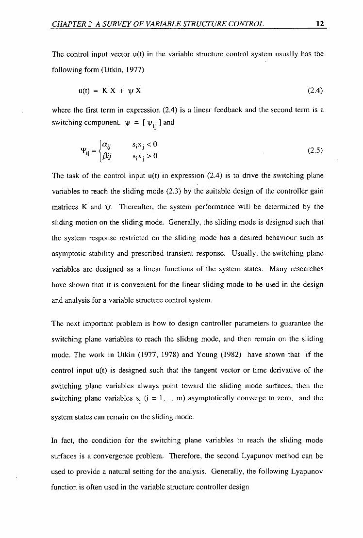
where the first term in expression (2.4) is a linear feedback and the second term is a switching component. w = [ wij 1 and
11/ — ía
M./ s i x j < 0 s i x j > 0
(2.5)
The task of the control input u(t) in expression (2.4) is to drive the switching plane
variables to reach the sliding mode (2.3) by the suitable design of the controller gain
matrices K and w. Thereafter, the system performance will be determined by the
sliding motion on the sliding mode. Generally, the sliding mode is designed such that
the system response restricted on the sliding mode has a desired behaviour such as
asymptotic stability and prescribed transient response. Usually, the switching plane
variables are designed as a linear functions of the system states. Many researches
have shown that it is convenient for the linear sliding mode to be used in the design
and analysis for a variable structure control system.
The next important problem is how to design controller parameters to guarantee the
switching plane variables to reach the sliding mode, and then remain on the sliding
mode. The work in Utkin (1977, 1978) and Young (1982) have shown that if the
control input u(t) is designed such that the tangent vector or time derivative of the
switching plane variables always point toward the sliding mode surfaces, then the switching plane variables s i (i = 1, m) asymptotically converge to zero, and the
system states can remain on the sliding mode.
In fact, the condition for the switching plane variables to reach the sliding mode
surfaces is a convergence problem. Therefore, the second Lyapunov method can be
used to provide a natural setting for the analysis. Generally, the following Lyapunov
function is often used in the variable structure controller design

CHAPTER 2 A SURVEY OF VARIABLE STRUCTURE CONTROL 13
1 V = —2 ST S (2.6)
In this case, the sufficient condition for the switching plane variables to reach the
sliding mode surfaces can be expressed as follows
• STS < 0 (2.7-a)
or
S. S. < 0 I (i = 1, m) (2.7-b)
It has been noted that most of the variable structure control algorithms are designed
based on the sufficient condition in expression (2.7-a) or expression (2.7-b) (Utkin,
1978 and DeCarlo, 1988).
2.2.2 Equivalent control
On the sliding mode, s = 0 and = 0 (i = 1, ...m). Then, using expressions (2.1) and
(2.2), we have
= CAX + CBueq = 0
(2.8)
where ueq is called as equivalent control.
If IC 1131# 0, the equivalent control u eq can be written as
ueq = -(CB) 1 CAX
=-KX (2.9-a)
where K = (C B) 1 C A (2.9-b)
CHAPTER 2 A SURVEY OF VARIABLE STRUCTURE CONTROL 14
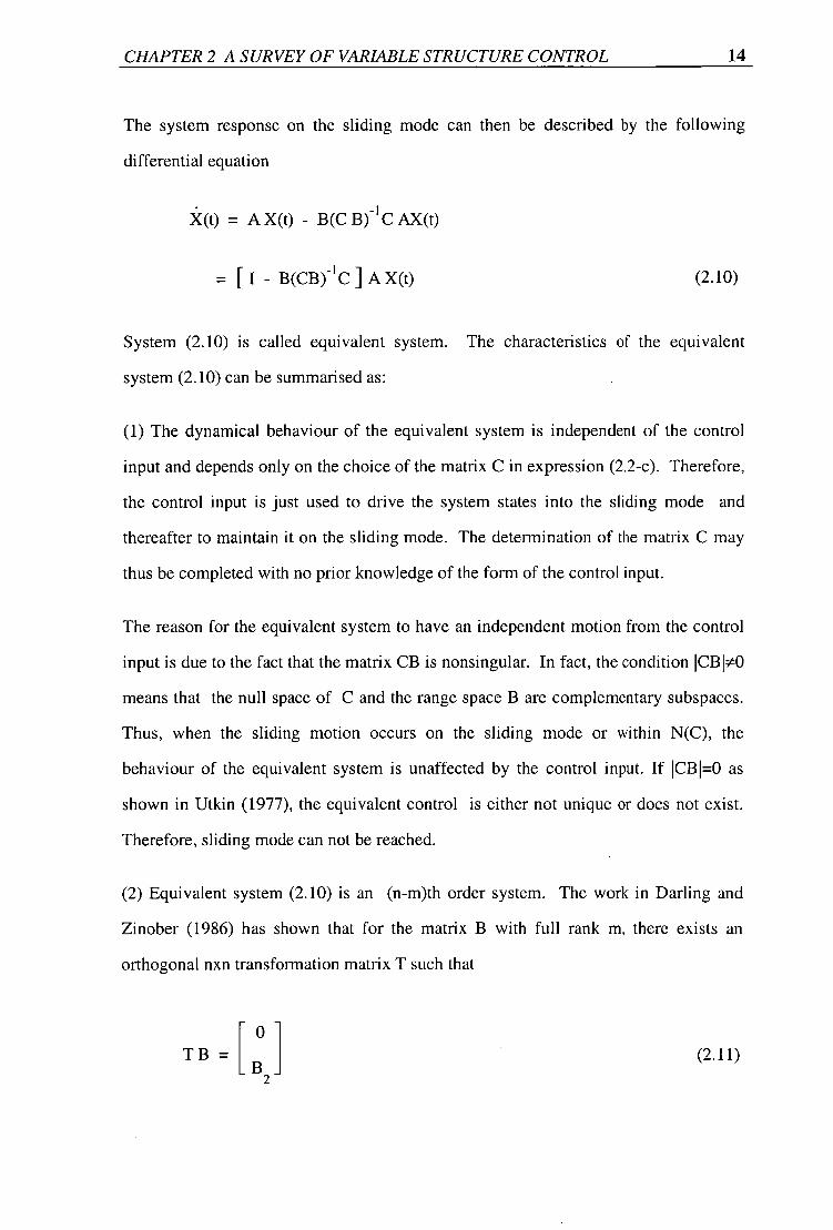
The system response on the sliding mode can then be described by the following
differential equation
X(t) = A X(t) - B(C B) AX(t)
= [ I - B(CB) -1 C A X(t) (2.10)
System (2.10) is called equivalent system. The characteristics of the equivalent
system (2.10) can be summarised as:
(1) The dynamical behaviour of the equivalent system is independent of the control
input and depends only on the choice of the matrix C in expression (2.2-c). Therefore,
the control input is just used to drive the system states into the sliding mode and
thereafter to maintain it on the sliding mode. The determination of the matrix C may
thus be completed with no prior knowledge of the form of the control input.
The reason for the equivalent system to have an independent motion from the control
input is due to the fact that the matrix CB is nonsingular. In fact, the condition ICBI#0
means that the null space of C and the range space B are complementary subspaces.
Thus, when the sliding motion occurs on the sliding mode or within N(C), the
behaviour of the equivalent system is unaffected by the control input. If 'CBI.° as
shown in Utkin (1977), the equivalent control is either not unique or does not exist.
Therefore, sliding mode can not be reached.
(2) Equivalent system (2.10) is an (n-m)th order system. The work in Darling and
Zinober (1986) has shown that for the matrix B with full rank m, there exists an
orthogonal nxn transformation matrix T such that
T B = (2.11)

CHAPTER 2 A SURVEY OF VARIABLE STRUCTURE CONTROL 15
where B 2 is an mxm nonsingular matrix.
Define a transformed state variable vector Y = T X, state equation (2.1) becomes
ir = TATT Y + TBu (2.12)
If Y is partitioned as
yT = i vT yT 1
L '1 '2 i
and matrices T A TT and CTT are partitioned as
TAT T =[A " A 21 A
Al2
22
1 C TT = [c 1 c2 ]
then, the system (2.12) can be written in the following form
Y = AYI + A 1 2 Y2 1
Y2 = AY1 + A2 2 Y2 -I- B 2 U
On the sliding mode, we have
C l Y 1 + C2 Y2 = 0
Or
Y2 = - F Y1
where
F = C-1 C 2 1
(2.13-a)
(2.13-b)
(2.13-c)
(2.14-a)
(2.14-b)
(2.15-a)
(2.15-b)
(2.15-c)

CHAPTER 2 A SURVEY OF VARIABLE STRUCTURE CONTROL 16
The equivalent system can then be written in the following form
= (A i - A l2 F) Y 1 (2.16)
Therefore, we can see from expression (2.16) that the equivalent system is (n-m)th
order system, i.e., the system dynamics is simplified on the sliding mode.
2.2.3 Robustness property
Robustness property is an important feature of a variable structure control system.
Suppose that system (2.1) has uncertainty in matrix A and external disturbance, then
the system state equation can be written in the following form
X(t) = (A0 + AA) X(t) + Bu + Df (2.17)
where A0 is the nominal system matrix, AA is the uncertainty, f E R L is a bounded
external disturbance vector, and matrix D is compatibly dimensioned. Without loss of
generality, it can be assumed that matrices B and D are full rank and the uncertainty
presented in the input distribution matrix B is incorporated in the system disturbance
term. During the sliding motion, the state vector of the system satisfies the following
equations
C X = 0
(2.18-a)
C(A + AA)X + CBueq + CDf = 0
(2.18-b)
From expression (2.18-b), the equivalent control can be achieved as
ueq = - ( CB ) -1 C ( AX + AAX + Df )
(2.19)
and the equivalent system equation is then given by

CHAPTER 2 A SURVEY OF VARIABLE STRUCTURE CONTROL 17
= [ I - B( CB ) -I C AX + AAX + Df ) (2.20-a)
CX = 0 (2.20-b)
Spurgeon (1991) has shown that the sliding mode system (2.20) is insensitive to
parameter variations and the external disturbance if and only if the system uncertainty
AA, matrices B and D satisfy the following rank relation
rank [ B : DI = rank [ B : AAT] = rank [B] (2.21)
where T is the matrix of the basis vectors of the reduced-order sliding subspace
defined by expression (2.20).
Expression (2.21) is also called as the invariance condition. In addition, the
robustness property for variable structure systems have been investigated by other
researchers. For example, Gutman (1979) and Bormish and Leitmann (1983) have
shown that if system uncertainties and disturbance satisfy the "matching condition",
then the system is completely insensitive on the sliding mode, and the effect of
disturbance and parameter variations can be minimised by minimising the time
required to attain the sliding mode.
2.2.4 Two methods of sliding mode design
Equivalent system equation (2.10) shows that the system behaviour on the sliding
mode depends only on the choice of the sliding mode parameter matrix C, and
asymptotic stability and desired transient response can be obtained by the suitable
design of matrix C. Usually, there are two methods for the sliding mode designs.
They are (a) the quadratic minimisation method and (b) the eigenstructure assignment
method.

CHAPTER 2 A SURVEY OF VARIABLE STRUCTURE CONTROL 18
The quadratic minimisation method for the sliding mode design was proposed by
Utkin and Young (1978). In this method, the following cost function is defined
J(u) = X(OTQX(t)dt (2.22)
where Q is a symmetric positive-definite matrix, and t s denotes the time at which the
sliding mode starts.
Partitioning the following matrix compatibly with Y (see subsection 2.2.2)
TTQT =[QH
where matrix T is defined
the cost function (2.22)
1 J(v) = —
2 t s
where
Q* = Q 1 1
A* = A11
v(t) = Y2
Y 1 = A* Y
Q21
Q12
Q22
in
can then
00
f YTI Q*
- Q 12 22%1
-0 iz --212
+ Q-1 Q21 22
1 + A12
expression (2.11),
be expressed in the following form
Y I + vTQ22V }dt
0 —21
Y 1
V(t)
(2.23)
(2.24)
(2.25-a)
(2.25-b)
(2.25-c)
(2.25-d)
Expression (2.24) is the form of standard linear quadratic optimal regulator problem.
By minimising expression (2.24), the optimal control v(t) is given by

CHAPTER 2 A SURVEY OF VARIABLE STRUCTURE CONTROL 19
v(t) = - Q-212ATI2PYI
Using expression (2.25-e) in expression (2.25-c), we have
(.1_1 r n A T 0, i v Y2 = - '22 1- '21 + '121 J i l = - FYI
where the matrix P satisfies the following Riccati equation
-1 n PQ* + A*P - PA l2(1 AT
22 1-'1210, ± `:
n = '
and matrix
-I r T 1 F = (222 1- Q2I + Al2 P -I
(2.25-e)
(2.26)
(2.27-a)
(2.27-b)
can then be determined as required.
The eigenstructure assignment method is also very popular in the sliding mode designs
and it was first used by Utkin and Young in 1978.
Suppose that the sliding mode has commenced on N(C). Then the equivalent system
can be written as
X(t) = (A - BK)X(t)
where matrix K is given in expression (2.9-b).
During the sliding motion, the state variables must remain in N(C) so that
C[ A - BK ] = 0 <=> R(A - BK) c N(C)
(2.28)
(2.29)
Let X i (i = 1, ... n) be the eigenvalues of A - BK with corresponding eigenvectors vi,
then, from expression (2.29), we have

CHAPTER 2 A SURVEY OF VARIABLE STRUCTURE CONTROL 20
C[ A - BK lv i = X.Cv. = 0 (2.30)
Expression (2.30) shows that either X i is zero or v i E N(C). Since A - BK = A eg has m
zero-valued eigenvalues, we can set { X i : i = 1, n-m } be the nonzero eigenvalues
and therefore, specifying the corresponding eigenvalues { v i : i = 1, n-m } fix the
null space of C (dim[N(C)] = n - m).
It is noted that C is not uniquely determined because the equation
CV = 0, V = [v 1 vn _ m (2.31)
has m2 degree of freedom, which may be easily seen if we define
W = [ 1= Tv (2.32) W2
where the partitioning of W is compatible with that of Y, then expression (2.31)
becomes
0 = CTT. Tv = [C I C2 ] [ W 2
1= C2 ( F —
[ W1 1 W2
Therefore, F can be determined from the following equation
FW 1 = - W2
(2.33)
(2.34)
The work of Dorling and Zinober (1986) has shown that this approach has the
drawback that the eigenvectors of matrix A-BK are not freely assignable, and at most
m elements of an eigenvector may be assigned arbitrarily, after which the remaining
n-m elements are fully determined by the assigned elements. Thus one approach to
eigenvector assignment is to select m elements according to some scheme and accept
the remaining elements as determined. This may allow a degree of adjustment to be
carried out by inspection.

CHAPTER 2 A SURVEY OF VARIABLE STRUCTURE CONTROL 21
Some other eigenvector assignment methods have also been proposed, and the details
can be found in Moore (1976), Klein and Moore (1977) and Sinswat and Fallside
(1977).
2.2.5 Controller designs
In most of the variable structure control schemes, the control law usually consists of a NL linear component uL and a nonlinear component u which are assumed to form
control input u. The linear part is merely a state feedback
= KX (2.35)
While the nonlinear signal incorporates the discontinuous elements of the control.
Some examples of possible types of nonlinearity are as given below.
(a) A nonlinear component with constant gains
NL u i = Mi sgn( C i X), M1 > 0
(b) A nonlinear component with state-dependent gains
NL MU. = i (X) sgn( C X ) m i (.) > 0
(2.36)
(2.37)
(c) A linear feedback with switching gains
uNL = TX
(2.38-a)
where 111 = [ tvii ] and
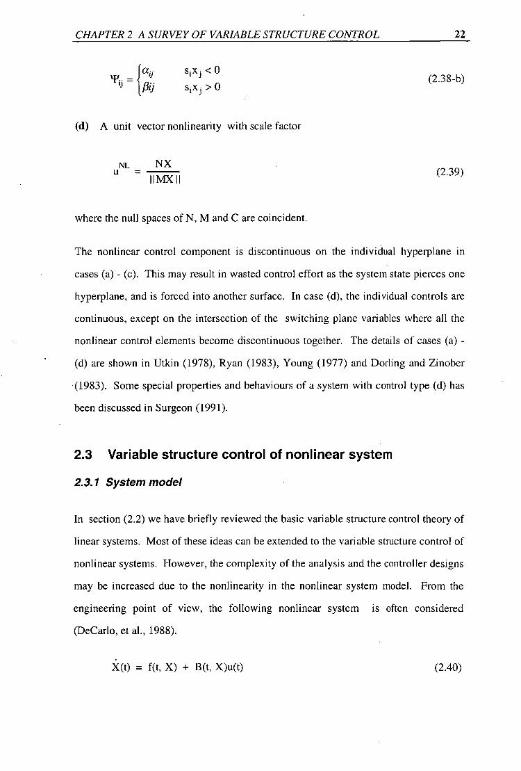
CHAPTER 2 A SURVEY OF VARIABLE STRUCTURE CONTROL 22
(d)
j =
A unit
NEL
•s l < 0
s i x > 0
vector nonlinearity with scale factor
NX
(2.38-b)
(2.39) Ilmx11
where the null spaces of N, M and C are coincident.
The nonlinear control component is discontinuous on the individual hyperplane in
cases (a) - (c). This may result in wasted control effort as the system state pierces one
hyperplane, and is forced into another surface. In case (d), the individual controls are
continuous, except on the intersection of the switching plane variables where all the
nonlinear control elements become discontinuous together. The details of cases (a) -
(d) are shown in Uticin (1978), Ryan (1983), Young (1977) and Dorling and Zinober
(1983). Some special properties and behaviours of a system with control type (d) has
been discussed in Surgeon (1991).
2.3 Variable structure control of nonlinear system
2.3.1 System model
In section (2.2) we have briefly reviewed the basic variable structure control theory of
linear systems. Most of these ideas can be extended to the variable structure control of
nonlinear systems. However, the complexity of the analysis and the controller designs
may be increased due to the nonlineatity in the nonlinear system model. From the
engineering point of view, the following nonlinear system is often considered
(DeCarlo, et al., 1988).
X(t) = f(t, X) + B(t, X)u(t) (2.40)
CHAPTER 2 A SURVEY OF VARIABLE STRUCTURE CONTROL 23
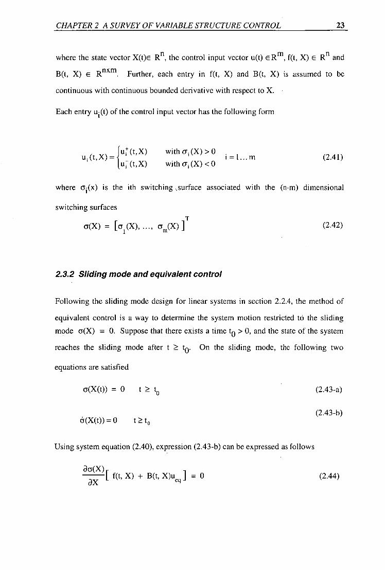
where the state vector X(t)E Rn , the control input vector u(t) E R m , f(t, X) E Rn and
B(t, X) E Rnxm. Further, each entry in f(t, X) and B(t, X) is assumed to be
continuous with continuous bounded derivative with respect to X.
Each entry u(t) of the control input vector has the following form
(t, X) u ; (t, X) = '
u (t, X) with cr i (X) > 0 with a ; (X) <0
(2.41)
whereis the ith switching ,surface associated with the (n-m) dimensional a t (x)
switching surfaces
a(X) = [a l (X), , szYm(X)
2.3.2 Sliding mode and equivalent control
Following the sliding mode design for linear systems in section 2.2.4, the method of
equivalent control is a way to determine the system motion restricted tO the sliding
mode a(X) = 0. Suppose that there exists a time t o > 0, and the state of the system
reaches the sliding mode after t to . On the sliding mode, the following two
equations are satisfied
cr(X(t)) = 0 t to
a(X(t)) =0 t t o
Using system equation (2.40), expression (2.43-b) can be expressed as follows
(2.43-a)
(2.43-b)
acy(x), f(t, X) + B(t, X)ueq = o ax (2.44)
(2.42)

CHAPTER 2 A SURVEY OF VARIABLE STRUCTURE CONTROL 24
where ueq is the so called equivalent control which can be obtained from expression
(2.44) as follows
-1 au(X) aa(x) U = - - ti(t, X) - f(t, X)
eq r
OX , ax (2.45)
Using expression (2.45) in system model (2.40), the dynamics of the closed loop
system on the sliding mode is given by
-1 acs(X) [ - B(t, X)( a(X)B( X)) f(t, X) ax ax (2.46)
Therefore, the problem of the sliding mode design is to choose the parameters in
a(X) = 0 such that the equivalent system (2.46) is stable. In most of variable structure
control schemes for nonlinear systems, the linear sliding modes are often used.
Therefore, some methods of sliding mode design in sections 2.2.4 can also be used.
2.3.3 Controller design
2.3.3.1 Diagonalisation method
In general, for nonlinear system equation (2.40), the control input is an m dimensional
vector and each entry has the structure of the form
u!," (t, X) u = _ u (t, X)
for a, (X) > 0 for a- , (X) < 0
(2.47)
To determine the switched feedback gains in control law (2.47), the following
diagonalisation method is often used (DeCarlo et al., 1988).
First, a new control vector is considered in terms of a nonsingular transformation

CHAPTER 2 A SURVEY OF VARIABLE STRUCTURE CONTROL 25
1 r aci ,
u*(t) = Q .(x)
.` (t, X) I_ - 113(t, X)u(t) ax
(2.48)
where Q-1 (t, X)(aa/aX)B(t, X) is a nonsingular transformation, and Q(t, X) is an arbitrary mxm diagonal matrix with elements q i(t, X) (i = 1, m) such that
inflqi (t, X)I > 0.
Using expression (2.48) in expression (2.40), the system dynamics becomes
= f(t, X) + B(t, X)1_ r aa(X)
B(t, X)-1
Q(t, X)u * (t) ax
If u* is selected such that
q i (t, X) u *: < - V o(X) f(t, X) ai (X) > 0
qi (t, X) u*i > - Vai (X) f(t, X) ai (X) < 0
(2.49)
(2.50-a)
(2.50-b)
then,
T (X)ã(X) <0
(2.51)
Expression (2.51) is the reaching condition for the system states to reach the sliding
mode surfaces a(X) = 0. On the sliding mode, the desired system dynamics can be
obtained. Also, the control input u(t) can be obtained from equation (2.48).
2.3.3.2 Reaching law method
In addition to the above diagonalisation method, the reaching law method (Gao and
Cheng, 1989; Gao and Hung, 1993) has been developed and proved to be efficient in
controller design. The reaching law is a differential equation which specifies the
dynamics of a switching function a(X). The differential equation of an asymptotically

CHAPTER 2 A SURVEY OF VARIABLE STRUCTURE CONTROL 26
stable a(X) is itself a reaching condition, i.e. a T (X)d(X) <0. In addition, by choice
of the parameters in the differential equation, the dynamic quality of VSC system in
the reaching mode can be controlled. A practical general form of the reaching law is
= —Q sgn(a) — Kh(a) (2.52)
where
Q = diag[q,,• • •,q], q, > 0
sgn(a) = [sgn(a,),• • •,sgn(a m K = diag[lc,,• • •, k], k, > 0
h(a) = [h i (a 1 ),•••,h m (a.)Ir 1 h 1 ( 1 )> O, h 1 (0)=
Three practical special cases of (2.52) are given below.
1) Constant rate reaching
= Q sgn(a) (2.53)
This law forces the switching variable a(X) to reach the sliding mode surfaces
a(X)=0 at a constant rate = —q 1 . The merit of this reaching law is its simplicity.
But, if q . too small, the reaching time will be too long. On the other hand, a q, too
large will cause severe chattering. In the following chapters of this thesis, a fuzzy
tuning algorithm for q, will be introduced to optimise the system performance.
2) Constant plus proportional rate reaching
= —Q sgn(a) — Ka (2.54)
Clearly, by adding the proportional rate term —Ka, the system state is forced to
approach the sliding mode surfaces a(X)=0 faster when a is large. It can be shown
that the reaching time for X to move from an initial state X 0 to the sliding surfaces is
finite, and is given by

CHAPTER 2 A SURVEY OF VARIABLE STRUCTURE CONTROL 27
1 kla. 1+q, T = ln "° .
k 1 q 1
3) Power rate reaching
6 = —1c 1 lada sgn(6 1 ), 0< a <1,i =1,...,m (2.55)
This power rate reaching law increases the reaching speed when the state is far away
from the sliding mode surfaces a(X)=0, but reduces the rate when the state is near the
surfaces. The result is a fast reaching and low chattering reaching mode. Integrating
(2.55) from a, = c a, = 0 yields
1 T, = la I 1 - Wki ( a), i = 1, m (2.56)
showing that the reaching time is finite.
The control law can be determined by the time derivative of a and the reaching law
(2.52), i.e.,
u =acY aX
B(t X)1 -1 r a' f(t, X) + Q sgn(a) + Kh(a)1 j Lax
-1 where the matrix [-a-CY is nonsingular. Lax
(2.57)
2.3.4 Robust control of nonlinear systems
In practical situations, the system dynamics of a nonlinear system is different from its
nominal system model due to parameter uncertainties. To represent parameter
uncertainties in the plant, the following state equation is considered (DeCarlo, 1988).
= [ f(t, X) + Af(t, X, r(t)) I + [ B(t, X) + B(t, X, r(t)) 11(0 (2.58-a)
where r(t) is a vector function of uncertain parameters.

CHAPTER 2 A SURVEY OF VARIABLE STRUCTURE CONTROL 28
In most of researches (Corless and Leitmann, 1981; Gutman and Palmor, 1982;
Peterson, 1985), the plant uncertainties Af and AB are assumed to lie in the image of
B(t, X) for all variables t and X (this is called "matching condition'). Then dynamic
equation (2.58-a) can be expressed as follows
= f(t, X) + B(t, X)u + B(t, X)e(t, X, r, u) (2.58-b)
where e(t, X, r, u) represents system uncertainties.
DeCarlo et al. (1988) shows that if e(t, X, r, u) is bounded by a positive function p(t)
II e(t, X, r, u)11 2 p(t) (2.59)
and control input has the following form
where
U = Ueq +u n
ueq = _ [ B(t, X) 1
-1 a [
cy at(X) ± a
a (x))f(t, x) ax
BT(t, X) Vx V(t, X) A Un — - T 2
p(t x) II B . (t, X) V,V(t, X) I I
(2.60-a)
(2.60-b)
(2.60-c)
A
p( t, X) = a + p(t, X)
(2.60-d)
[ a6(t, X) ]T V xV(t, X) = a(t, x)
ax (2.60-e)
then system state can reach the sliding mode surfaces cr(X) = 0, and the desired system
dynamics can be obtained by the suitable choice of the sliding mode parameters.

CHAPTER 2 A SURVEY OF VARIABLE STRUCTURE CONTROL 29
The results discussed in this section forms the foundation of the variable structure
control theory for nonlinear systems. Although there are many classes of nonlinear
systems, robustness and convergence of variable structure control systems may be
established based on the results in this section (Utkin, 1978; Young, 1978 and
DeCarlo et al., 1988).
2.4 Application to robot manipulators
A robotic manipulator is a typical nonlinear system. The investigations for the control
of robotic manipulators have not only improved the robotic system performance, but
also developed many new control techniques which have enhanced the modern control
theory. Many control schemes such as feedback control and adaptive control have
been developed for robotic manipulators. However, the variable structure control
technique is one of the most powerful techniques due to the fact that the variable
structure control can deal with systems with large uncertainties, bounded disturbances
and nonlinearities. In recent years, the designs of robust variable structure control
laws for rigid robotic manipulators that ensure robustness and asymptotic trajectory
tracking have been investigated by many researchers. Many robustness and
convergence results have been obtained by Young (1978, 1988), Morgan and Ozguner
(1985), Slotine and Sastry (1983), Yeung (1988) and Leung et al (1991). In this
section, the dynamics of the robotic manipulator and a robust variable structure
controller design using the reaching law method (Gao and Hung, 1993) will be
presented to highlight the main issues of the control scheme.
2.4.1 Dynamics of robotic manipulators
In the absence of friction and other disturbances, the joint space dynamics of an n-link
robotic manipulator can be written via the so-called Eular-Langrange equations as
(Spong and Vidyasagar, 1988):

CHAPTER 2 A SURVEY OF VARIABLE STRUCTURE CONTROL 30
dkj (q) + fijk (q) + (q) = T ic k = 1, n (2.61)
where dk . are the coefficients of the inertia matrix D(q), k(q) are the gravitational
forces and T ic are the input torques. The coefficients f of the coriolis and centrifugal
terms are defined as
ad ki ad,„ ad ii } aq; aq; aq k
1 fijk = (2.62)
and f are known as Christoffel symbols.
It is common to write expression (2.62) in matrix form as
D(q) + F(q, 4 + G(q) '= (2.63)
where the k,jth element of the matrix F is defined as
n AA ad.. . f = I _adki _ )(11 kJ 2k. -_,
i=1 oqi aqi aqk (2.64)
and the component of G(q) is Ok .
Although the equation of motion (2.63) is complex and nonlinear for all but simple
robotic manipulators, it has several fundamental properties which can be exploited to
facilitate control system design (Ortega and Spong, 1989).
Property 1: The inertia matrix D(q) is symmetric, positive-definite, and both D(q)
and D(q)4 are uniformly bounded as a function of q.
Property 2: There is an independent control input for each degree of freedom.
Property 3: The Euler-Lagrange equation for the robotic manipulator is linear in the
unknown parameters. All the unknown parameters are constant (e.g. link masses, link
lengths, moments of inertia, etc.) and appear as coefficients of known functions of the

CHAPTER 2 A SURVEY OF VARIABLE STRUCTURE CONTROL 31
generalised coordinates. By defining each coefficient or a linear combination of them
as a separate parameter, a linear relationship results so that we may write equation
(2.63) as
D(q) 4 + F(q, q) 4 + G(q) = Y(q, q, 4)o = (2.65)
where Y is an nxr matrix of known functions, known as the regressor, and q is a n
dimensional vector of unknown parameters as shown in Spong and Vidyasagar (1989).
It can be seen later that the manipulator system (2.63) can also be expressed into the
generalised form in expression (2.40). Therefore, the basic variable structure theory
can be used to design robust controllers and the structural properties mentioned in the
above can then be used to simplify controller designs.
2.4.2 A robust VSC controller design
Consider an n-link manipulator system with perturbations and disturbances described
by
D(q)4 + F(q, q)q + G(q) = w(q, q, p, t) (2.66)
where p is an uncertain parameter vector, w(q,q, p, t) is the collection of all system
perturbations and external disturbances. The state variable is defined as
X = {q T T (2.67)
Then (2.66) can be put into the form
X = f(t, X) + B(t, X)u + v(X, p, t) (2.68)
where
U = T, 0
v(X, p, t) = [ D -1 (q)w(X, p,

CHAPTER 2 A SURVEY OF VARIABLE STRUCTURE CONTROL 32
f(t, X) = (q)(F(q, q)q + G(q))
1'
B (t X) = [ (q)].
The arm is to track a desired motion Cl d (t). The output tracking error is defined as
= d e = [ET •11T (2.69)
The sliding mode surfaces are chosen as
a(e) = Ce = [A 11[]= Ac (2.70)
Adopt the reaching law
= sgn(a) Ka
Taking the time derivative of (2.70) gives
(2.71)
eT=At+
=Ae+qd +D-I (Fq+G—w—u) (2.72)
• Equating (2.71) and (2.72) and solving for the control u yields
u = D{Qsgn(a)+ Ka + Ae + q d } + Fq +G — w (2.73)
All quantities on the right-hand side of (2.73) are known except the disturbance w,
which is unknown. To cope with this problem, define
w 1 =1:30 -1 w
and assume that w 1 is bounded by
(2.74)
(2.75)
Then replace w in (2.73) by —DW sgn(a) give following control law
u = D{Q sgn(a) + Ka + Ae + q d } + Fq + G + DT/ sgn(a)
Substituting (2.76) into (2.72) give
(2.76)

CHAPTER 2 A SURVEY OF VARIABLE STRUCTURE CONTROL 33
6 = —Q sgn(a) — Ka — w 1 — sgn(a) (2.77)
Thus, the reaching condition a T6 < 0 is guaranteed.
This robust controller design is based on the bounding function estimation of the
system perturbations and external disturbances, and the exact system knowledge is not
required. However, the system performance and control quality depend very much on
the choice of sliding mode parameter Q and the estimation of bounding function of the
unknown parts. Excessive control torques and severe control chattering may be easily
caused by over estimation of control parameters.
In order to overcome these shortcomings, in chapter 5 of this thesis, fuzzy logic
technology will be used to dynamically adjust the sliding mode parameter Q, and
control chattering will be reduced dramatically. In chapter 8, a robust adaptive control
scheme for robots is established where neural network has been constructed to
adaptively learn the bounding function of the unknown parts of the robot system.
2.5 Concluding remarks
The basic theory of variable structure control systems has been briefly surveyed in this
chapter. Because the variable structure theory has many good features, it can be
easily used to control linear or nonlinear systems. Although the robustness can be
achieved without the exact knowledge of the control system, the system performance
and control quality depend very much on the choice of sliding mode parameters and
the estimation of bounding functions of the unknown parts. In practice, excessive
control input and severe control chattering which may excite unmodelled high-
frequency dynamics are highly undesirable. In the following chapters of this thesis,
several new and improved robust variable structure control schemes of nonlinear
systems will be proposed by combining conventional methods and recently developed

CHAPTER 2 A SURVEY OF VARIABLE STRUCTURE CONTROL 34
techniques, namely fuzzy logic and neural networks, to improve the system
performance and enhance the control quality.

CHAPTER 3 FUZZY LOGIC AND FUZZY LOGIC CONTROL 35
Chapter 3
Fuzzy Logic and Fuzzy Logic Control
3.1 Introduction
Zadeh (1965) published his first paper on a novel way of characterising
nonprobabilistic uncertainties, which he called "fuzzy sets". Fuzzy logic and fuzzy set
theory has now evolved into a fruitful area containing various disciplines, such as
calculus of fuzzy if-then rules, fuzzy graphs, fuzzy interpolation, fuzzy topology,
fuzzy reasoning, fuzzy inference systems, and fuzzy modelling. The applications,
which are multi-disciplinary in nature, include automatic control, consumer
electronics, signal processing, time-series prediction, information retrieval, database
management, computer vision, data classification, decision-making, and so on.
Within the diverse areas of fuzzy logic applications, control is the area to which fuzzy
systems are most widely applied today. The genesis of fuzzy logic control was a paper
by Chang and Zadeh (1972) outlining the basic approach. An important landmark in
this development was the introduction of linguistic 'variables whose values are
linguistic terms rather than numbers (Zadeh, 1973). Fuzzy technology, Zadeh

CHAPTER 3 FUZZY LOGIC AND FUZZY LOGIC CONTROL 36
explained, is a means of computing with words for which the role model is the human
ability to reason and make decisions without the use of numbers (Zaheh, 1996). The
first implementation of these ideas was described in a paper by Mamdani (1974). The
key principle underlying fuzzy logic control is based on a logical model which
represents the thinking process that an operator might go through to control the system
manually. The viability of fuzzy logic control has been demonstrated through wide-
spread applications (Schwartz et al, 1994). Fuzzy logic control can be considered as
one of the intelligent control techniques wherein engineering knowledge is reflected in
the controller. It has been found that such controllers have definite advantage over the
traditional HD controllers in that they are more robust with respect to structured or
unstructured uncertainties. The linguistic characteristics of fuzzy control provide a
very good approach to account for the sensor noise, unmodelled dynamics, parameter
variations, disturbances and nonlinearities (Lee, 1990).
It is known that the classical P1D controllers do not work very well for the case of
nonlinear control and, even for linear control they typically have to be redesigned
according to a new set of basic system parameters. Adaptive controllers have been
proposed for these systems. By means of some tuning scheme, the controller
parameters can be continuously adjusted to improve robustness against any changing
environment. Auto-tuning (Astrom et al ,1992) or auto-calibration (Voda and Landau,
1995) of controllers for plants with uncertainties is useful although some knowledge
of the process is needed. Tuning the controller parameters to achieve better
performance can be accomplished by means of fuzzy logic (Tseng & Hwang, 1993).
A smooth control signal can be achieved by fuzzy tuning of the discontinuous control
component in the sliding mode control (Mei & Man et al, 1998), where control

CHAPTER 3 FUZZY LOGIC AND FUZZY LOGIC CONTROL 37
chattering is an undesirable disadvantage inherent to conventional sliding mode
control.
In recent years, fuzzy modelling of controlled systems has received much attention. A
number of researchers (Feng and Cao et al, 1997; Tanaka et al, 1996) proposed fuzzy
global systems with stability analysis based on Takagi-Sugeno fuzzy inference model.
Mei & Man et al (1998) presented a fuzzy modelling and robust tracking control
scheme for a class of nonlinear systems by fuzzifying over a number of operating
points within the interested range.
Despite a large number of technical publications focusing on fuzzy systems, there
exist some doubtful opinions on fuzzy controllers mainly due to some
misunderstanding about fuzzy control. Attempts have been made to clear up this
misunderstanding, e.g. Jager (1995). It is, therefore, of interest to start the notable part
of this thesis, with a short primer on fuzzy set theory, fuzzy reasoning, and fuzzy logic
control, using fuzzy tool in combination with other techniques.
The arrangement of this chapter is as follows. Section 3.2 gives the definitions of
fuzzy sets, fuzzy set operations, fuzzy relation and compositions, and linguistic
representations. Section 3.3 describes fuzzy logic and fuzzy reasoning. Section 3.4
introduces fuzzy logic control.
3.2 Fuzzy set theory
Due to the rapid growth of fuzzy logic literature, it is difficult to present a
comprehensive survey of its wide applications. A lot of them are too theoretical to be

CHAPTER 3 FUZZY LOGIC AND FUZZY LOGIC CONTROL 38
applied to engineering problems. The purpose of this section is to briefly summarise
the basic concepts that are necessary in understanding fuzzy logic and fuzzy inference
from a practical viewpoint.
3.2.1 Fuzzy sets
A universe of discourse (or domain of definition) U is the set of allowable values for a
variable, denoted generically by {x} which could be discrete or continuous, where x
represents the generic element of U.
A crisp set A in a universe of discourse U can be defined as A = {xi (x)} where
/A A (x) is, in general, a condition by which x e A. If we introduce a zero-one
characteristic function such that A = 02 A (x) = 1 if x e A and // A (x)= 0 if x 0 A) then
/L A (X) is called a membership function for A.
A fuzzy set F in a universe of discourse U is characterised by a membership function
kt F (x) which takes on values in the interval [0, 1]. A fuzzy set may be viewed as a
generalisation of the concept of an ordinary (i.e. crisp) set whose membership function
only takes two values {0, 1}. A membership function for a fuzzy set F provides
a measure of the degree of similarity of an element in U to F. A fuzzy set F in U may
be represented as a set of ordered pairs of a generic element x and its grade of
membership function: F = ((x„ u F (x))1x ctn. When U is continuous, F can be
written concisely as F = fu ,uF(x ) Ix, where the integral sign denotes the collection of
all points x E U with associated membership function I, F (x). When U is discrete, F is
represented as F= E ttF (xxx„ where the summation sign stands for the union of XiEU
(x, I F (x)) pairs. Similarly, the slash "I" in these expressions is only a marker and

70 90 100 weight(kg) 40 50
Degree of membership
LIGHT HEAVY
0.5 crossover pclint
0
CHAPTER 3 FUZZY LOGIC AND FUZZY LOGIC CONTROL 39
does not imply division. Note that in fuzzy sets, an element can reside in more than
one set to different degrees of similarity. This cannot occur in a crisp set theory.
The support of a fuzzy set F is the crisp set of all points x E U such that /.2 F (x)> 0.
The element x E U at which ki F (x) = 0.5 is called the crossover point. For example,
the formal domain for normal weight might be 40 to 100 kg. However, the fuzzy sets
HEAVY and LIGHT can have non-zero membership grade at 50 to 90 kg with a
crossover point at 70 kg, as shown in Fig. 3.1. A fuzzy set whose support is a single
point x in U with /./ F (x) =1 is referred to as fuzzy singleton. In a singleton output
space, fuzzy set membership functions are represented as single vertical points.
Figure 3.2 illustrates how a variable SPEED can be composed on individual single
points.
support
universe of discourse
Fig. 3.1 Fuzzy variable "weight"

CHAPTER 3 FUZZY LOGIC AND FUZZY LOGIC CONTROL 40
A 11(x)
1
0 ■ 40 60 80 speed(km1 h)
Fig. 3.2 Singleton representation.
3.2.2 Set theoretical operators (Lee, 1990)
Let fuzzy sets A and B in U be described by their membership functions ,u A (x) and
14, B (x). The set theoretic operations of union, intersection and complement for fuzzy
sets are defined as following.
Union (disjunction): The membership function R AL, B of the union A u B (A OR B) is
pointwise defined for all x E U by
AuB(x) =max(R A (x), 1u 8 (x)} (3.1) P
Intersection (conjunction): The membership function ,L1An/3 of the intersection A n B
(A AND B) is pointwise defined for all x E U by
ktiar,B(x)= min{,u A (x), ,u 8 (x)} (3.2)
Complement (negation): The membership function R A of the complement of a fuzzy
set A, -A (NOT A), is pointwise defined for all X E U by
,u-A (x) = 1 - RA (x) (3.3)

10
0.8
0.6
0.4
0.2
0o 5
(a)
0.8
0.6 -
0.4 -
0.2 -
0o
1
0.8
0.6
0.4
0.2
0o
5 (b)
5 (d)
10
10
CHAPTER 3 FUZZY LOGIC AND FUZZY LOGIC CONTROL 41
Fig. 3.3 illustrates these three basic operations: a) illustrates two fuzzy sets A and B,
b) is the complement of A, c) is the union of A and B, and d) is the intersection of A
and B.
Fig. 3.3 Operations on fuzzy sets: (a) two fuzzy sets A and B; (b) A; (c) AuB;(d) AnB.
Note that other consistent definitions for fuzzy AND and OR have been proposed in
the literature under the names "T-norm" and "T-conorm" operators (Mendel, 1995),
respectively.
T-norm: a t-norm, denoted by *, is a two-place function from [0, 1] x [0, 1] to [0, 1],
which includes fuzzy intersection, algebraic product, bounded product, and drastic
product, defined as

CHAPTER 3 FUZZY LOGIC AND FUZZY LOGIC CONTROL 42
mil-0,A,
xY, max(0, x + y — 1}, x if y = 1 yif x=1 ,
0 if x, y <1
fuzzy intersection algebraic product bounded product
drastic product
x* y =
where x, y E [0,1] .
T-cononn: A t-conorm, denoted by ®, is a two-place function from [0, 1] x [0, 1] to
[0, 1], which includes fuzzy union, algebraic sum, bounded sum, and drastic sum,
defined as
x@y=
- max{x, y}, fuzzy union x + y— xy, algebraic sum minfl, x + yl , bounded sum x if y = 0 y if x = 0 drastic sum
‘. lifx,y>0
where x, y e [0,1].
3.2.3 The extension principle
The extension principle is a tool for generalising crisp mathematical concepts to fuzzy
sets. It has been extensively used in the fuzzy literature.
The extension principle: Let U and V be two universe of discourse and f be a mapping
from U to V. For a fuzzy set A in U, the extension principle defines a fuzzy set B in V
by
11 B (Y) = suPxEr t (y) [UA (x)]
(3.4)

CHAPTER 3 FUZZY LOGIC AND FUZZY LOGIC CONTROL 43
That is, ,u B (y) is the superium of At A (x) for all x E U such that f(x)=y, where
y E Vand we assume that f -1 (y) is not empty. If f -1 (y) is empty for some y E V,
define /4 8 (y)=0.
3.2.4 Fuzzy relations and their compositions
Cartesian product: If An are fuzzy sets in , respectively, the Cartesian
product of A1 ,..., An is a fuzzy set in the product space u, x...xu with the membership
function
YA I x...xA„ = mintgA, (xn )1
(3.5a)
Or
(x i ,. ..,x) = (x, )...,uAn(xn)
(3.5b)
Fuzzy relations: Fuzzy relations represent a degree of presence or absence of
association, or interconnection between the elements of two or more fuzzy sets. An n-
ary fuzzy relation is a fuzzy set in u,x...xu„ and is expressed as
x..xu = ((x 1 ,..., ), /4 R ((x 1 ,...,x ) E U 1 x...xUn 1. (3.6)
Compositions: Because fuzzy relations are fuzzy sets in the product space, set
theoretic and algebraic operations can be defined using operators for fuzzy union,
intersection and complement. Let R and S be fuzzy relations in U x V. The
intersection and union of R and S, which are compositions of the two relations, are defined as
Rns (x, =
and
ktRus (x, Y) =
(3.7a)
(3.7b)
respectively, where * is any t-norm, and CI is any t-conorm.

y E V Z E W X E U
p. (x, • Ps(y,
CHAPTER 3 FUZZY LOGIC AND FUZZY LOGIC CONTROL 44
Next, consider the composition of fuzzy relations from different product space that
share a common set. If R and S are two fuzzy relations in U x V and V x W,
respectively, the sup-star composition of R(U x V) and S(V x W) is a fuzzy relation
denoted by R o S(U x V) and is defined by
Ro S = {(x,y), SUpLu R (x,Y)* ius(Y,z)l, x EU, y E V, Z E (3.8) yEV
where* could be any operator in the class of t-norm (the sup-product is most
commonly used). When U, V and W are discrete universe of discourse, the sup
operation is the maximum. Fig. 3.4 depicts a block diagram for the sup-star
composition.
Fig. 3.4. Block diagram interpretation for the sup-star composition.
Suppose fuzzy relation R is just a fuzzy set, then it R (X , y) becomes it R (X) and V=U,
consequently, sup[kt R (X, y)* s (y,z)]= R (X)* s (y,z)]. Thus, when R is just a yEV XEU
fuzzy set, the membership function for R o S is
■11 Ros (Z) = SUPU R (X)* S (Y Z)]
(3.9) XEU
Fig. 3.5 represents the block diagram interpretation for the sup-star composition when
the first relation is just a fuzzy set.

CHAPTER 3 FUZZY LOGIC AND FUZZY LOGIC CONTROL 45
V = U Z E W
(x) ,us(y,z)
J1-1 Ros(x , z)
Fig. 3.5. Sup-star composition when V = U.
3.2.5 Linguistic representation
A. Linguistic variables
The use of fuzzy sets provides a basis for a systematic way for the management of
vague and imprecise concepts. According to Zadeh (1975), in retreating from
precision in the face of overpowering complexity, it is natural to explore the use of
what might be called Linguistic variable, i.e., variables whose values are not numbers
but words or sentences in a natural or artificial language. Fuzzy sets can be employed
to represent linguistic variable. Consider a real line as a continuous universe of
discourse U. A fuzzy number F in U is a fuzzy sets which is normal and convex, i.e.,
max kt F (X) = 1 x€11
(3.10a)
F (Axi + A)x2 ) ?_ (x i ), P F (x 2 )), x, , X2 E u, E [OM. (3.10b)
A linguistic variable can be regarded as a variable whose value is a fuzzy number or
whose values are defined in linguistic terms or labels. A linguistic variable is
characterised by its name u; the term set of u, i.e., the set of terms T(u) of linguistic
values of u with each value being a fuzzy number defined on U; a syntactic rule for
generating the names of values of u; and a semantic rule for associating with each
value its meaning. For example, let SPEED (u) of a car be linguistic variable. It can be
decomposed into the following set of terms T(u)={ slow, medium, fast}, where each
term is characterised by a fuzzy set in the universe of discourse U 40 km/h, 100

CHAPTER 3 FUZZY LOGIC AND FUZZY LOGIC CONTROL 46
km/h]. "Slow" speed might be interpreted as "a speed below about 40 km/h",
"medium" as "a speed close to 60 km/h", and "fast" as "a speed above 80 km/h".
These terms can be characterised as fuzzy sets whose membership functions are
shown in Fig.3.6. A vertical line from any measured value of speed intersects at most
two membership functions. So, for example, a speed of 45 km/h resides in the fuzzy
sets slow and medium to a similarity degree of 0.75 and 0.25, respectively.
Pt speed
1.0
0 40 60 80 Speed (km/h)
Fig. 3.6 Membership functions of three fuzzy sets, namely, "slow", "medium", "fast" for the speed of a car.
B. Hedges: Linguistic modifiers
A Linguistic hedge or modifier is an operation that modifies the meaning of a fuzzy set
or a term. Hedges can be viewed as operators that act upon a fuzzy's set membership
function to modify it. Hedges play the same role in fuzzy modelling system as adverbs
and adjectives do in a nature language. Accordingly, the number and order of hedges
are significant, e.g. not very large and very not large relates to two different
interpretations. A representative collection of commonly-used hedges with their
effects is contained in Table 3.1 (Cox, 1994).

CHAPTER 3 FUZZY LOGIC AND FUZZY LOGIC CONTROL 47
Hedge Meaning
about, around, near, roughly Approximate a scaler above, more than Restrict a fuzzy region
almost, definitely, positively Contrast intensification
below, less than Restrict a fuzzy region
vicinity of Approximate broadly
generally, usually, normally Contrast diffusion
neighbouring, close to Approximate narrowly
not, not-so, not really Negation or complement
quite, rather, somewhat, Dilute a fuzzy region
more-or-less
very, extremely Intensify a fuzzy region
Table 3.1 Fuzzy linguistic hedge and their approximate meanings.
Power hedges (Zimmermann, 1985): The power hedges operate on grades of
membership and represented by the general operator:
,upow ( u ) (x) Diu (x )1P , (3.11)
where p is a parameter specific to a certain linguistic modifier. The exponent p used in
the hedge membership function is quite arbitrary, it can be changed depending on our
interpretation of the hedge. If p=1, fuzzy set is not modified. Two cases are
distinguished:
1)Concentration: p >1, fuzzy set is concentrated. Because membership functions are
assumed to be normalised, the operation of concentration leads to a membership
function that lies within the membership function of original fuzzy set; both have the
same support, and the same membership values where the value of the original
membership function equals unity or zero.
The modifier very corresponds to p=2. For example, if slow speed is fuzzy set with membership function /I s (x) , then very slow speed and very very slow speed are fuzzy

CHAPTER 3 FUZZY LOGIC AND FUZZY LOGIC CONTROL 48
sets with membership function La s (x)] 2 , [It s (x)] 4 , respectively. An artificial hedge
providing milder degree of concentration is the plus, whose membership function is
2) Dilation: p<1, fuzzy set is dilated. The operation of dilation leads to a membership
function that lies outside of the membership function of the original fuzzy set; both
have the same support, and the same membership values where the value of the
original membership function equals unity or zero.
The modifier more or less corresponds to p=1/2. For example, more or less slow speed
is a fuzzy set with membership function [u 5 (x)] "2 . Another hedge quite useful is the
minus, whose membership function is p,„„nus(u) (x)
3.3 Fuzzy logic and fuzzy reasoning
Fuzzy logic is a logical system that is much closer in spirit to human thinking and
natural language than traditional logic systems. As a calculus of compatibility, fuzzy
logic is quite different from probability which is based on frequency distributions in a
random population. Fuzzy logic describes the characteristic properties of continuously
varying values by associating partitions of these values with a semantic label (Cox,
1994). Fuzziness is different from probability. The laws of contradiction and excluded
middle are broken in fuzzy logic but are not broken in probability. Conditional
probability, which must be defined in probability theory, can be derived from first
principles using fuzzy logic (Kosko, 1992). Much of the description power of fuzzy
logic comes from the fact that these semantic partitions can overlap (see Fig. 3.6)
corresponding to the transition from one term to the next.
Fuzzy set serves as the basis for fuzzy logic. Fuzzy set theory starts with some basic
concepts coming from crisp set theory, fuzzy logic also begins by borrowing some
crisp logic notions. In crisp logic, a proposition is an ordinary statement involving
terms already defined, and must be meaningful to call it "true" or "false". A tautology
is a proposition formed by combining other propositions p, q, r,... .

CHAPTER 3 FUZZY LOGIC AND FUZZY LOGIC CONTROL 49
Let us start with the basic primitives of fuzzy logic: fuzzy propositions. A fuzzy
proposition represents a statement like "speed (u) is SLOW", where SLOW is a
linguistic label, defined by a fuzzy set on the universe of discourse of speed. Fuzzy
propositions connect variables with linguistic labels defined for those variables. As in
classical logic, fuzzy propositions can be combined by using logical connectives and
and or, which are implemented by t-norms and t- conorms, respectively.
Fuzzy logic provides a means of modelling human decision making within the
conceptual framework of fuzzy logic and approximate reasoning (or fuzzy reasoning).
In fact, reasoning with fuzzy logic is based on fuzzy rules which are expressed as
logical implications, i.e. in the forms of IF-THEN statements. In fuzzy logic, the
definition of a fuzzy implication may be expressed as a fuzzy implication function.
Various implication functions can be classified into three main categories: fuzzy
conjunction, fuzzy disjunction, and fuzzy implication. A fuzzy rule "IF u is A, THEN v
is B", is represented by a fuzzy implication and is denoted by A --> B, where A and B
are fuzzy sets in the universes U and V with membership functions /I A and u 8 ,
respectively. Membership function of the fuzzy implication, denoted by ,u 8(X0))1
measures the degree of truth of the implication between x E U and y E V.
Fuzzy conjunction: The fuzzy conjunction is defined for all x E U and y E V by
A —> B=A*B , (3.12)
where * is an operator representing a t-norm.
Fuzzy disjunction: The fuzzy disjunction is defined for all x E U and y E V by
A —> B=A0B (3.13)
where CI is an operator representing a t-conorm.

CHAPTER 3 FUZZY LOGIC AND FUZZY LOGIC CONTROL 50
Fuzzy implication: An extension is made by determining the fuzzy versions of some
tautologies of p—>q in crisp logic, e.g. -pvq,-pv pq, and (- pA -q)vq. Thus,
the fuzzy implication is associated with the corresponding families of fuzzy
implication functions:
(1) Material implication:
A —> B =not A (-) B (3.14)
(2) Propositional calculus:
A —> B =not ACI (A* B) (3.15) --,
(3) Extended propositional calculus:
A— B=( not A* not B) ,0 B (3.16)
In traditional propositional logic there are two very important inference rules, Modus
Ponens (MP) and Modus Tollens (MT). Modus ponens is associated with the
implication [ A —> B]:
Consequence Premises
Premise 1: x is A Premise 2: If x is A THEN y is B
y is B
In terms of propositions p and q, modus ponens is expressed as (p A (p —> q))—> q.
Modus tollens is associated with the implication [( not A --> not B)
Consequence Premises
Premise 1: y is B Premise 2: If x is A THEN y is B
x is not A

CHAPTER 3 FUZZY LOGIC AND FUZZY LOGIC CONTROL 51
In terms of proposition p and q, modus tollens is expressed as (— q A (p —> p.
In fuzzy logic, modus ponens is extended to Generalised Modus Ponens (GMP):
Consequence Premises
Premise 1: x is A* Premise 2: If x is A THEN y is B
y is B*
and modus tollens to Generalised Modus Tonens (GMT):
Consequence Premises
Premise 1: y is B* Premise 2: If x is A THEN y is B
x is A*
where A, A*, B, B* are fuzzy sets introduced via linguistic variables x, y (Dubois and
Prade, 1984). Two more families of fuzzy implication function obtained from GMP
and GMT are:
(4) Generalisation of modus ponens:
A —> B=supfc E [0,1], Mc B1 (3.17)
(5) Generalisation of modus tollens:
A —> B=inflt E [0,1], Bt AI (3.18)
Based on the definition (3.12-3.18), many membership functions for fuzzy implication
may be generated by employing appropriate triangular norms and conorms. For
example, kt A-o B (X v) can be found from (3.14) as
=
A,B (x, y) = 1- A (x),1– kiB(Y)1,

CHAPTER 3 FUZZY LOGIC AND FUZZY LOGIC CONTROL 52
Or
PA,B(x, y) = 1- IL A (x)(I - ilB(Y)) (3.19c)
with appropriate operators for the t-norm * and t-conorm CI . From the fuzzy
conjunction (3.12), membership function for minimum implication, proposed by
Mamdani (1974):
P A-4 8 (X ' Y) min[11 A (x),/-1 B (Y)]
and product implication, introduced by Larsen (1980):
il A,B (x, Y) =- ItA (x),/-tB (Y)
(3.20)
(3.21)
can be obtained using minimum and algebraic product, respectively. It can be shown
that membership functions (3.19a-c) agree with the accepted propositional logic
definition of implication, demonstrated in Table 3.2 while neither Mamdani
membership function (3.20) nor Larsen one (3.21) does. As shown in Table 3.2,
minimum and product inferences preserve cause and effect, i.e. these implications are
fired only when the antecedent and the consequent are both true.
kip (x) 11 , (x) lip,, (x, Y) min[PLA (x),11 8 (Y)] 1-1 ,1 (x),u B (Y)
.-.1
I-I C
) v-
I
1 1
...-
CD 0 0
0 0 0 0
Table 4.2 Implication with propositional logic, and min and product inference.
This is why minimum and product inferences are the most widely used inferences in
engineering applications of fuzzy logic, and referred to as engineering implications
(Mendel, 1995).
A comprehensive comparison between the available fuzzy implication rules is given in
Lee (1990), based on some intuitive criteria for choosing a fuzzy implication that is as

CHAPTER 3 FUZZY LOGIC AND FUZZY LOGIC CONTROL 53
close as possible to the input truth value function value. Although the minimum
operation rule (3.20) and the product operation rule (3.21) of fuzzy implication do not
have a well-defined logic structure, it is shown (Lee, 1990) that they are well suited
for approximate reasoning, especially for the generalised modus ponens. The GMP,
reducing to modus ponens when A* =A, B* =B, is closely related to the forward data-
driven inference, particularly used in control system. The GMT, reducing to modus
tollens when A* =not A, B* =not B, is closely related to the backward goal-driven
inference, commonly used in expert systems.
Fig. 3.7 illustratively interprets that GMP is a fuzzy composition where the first fuzzy
relation is merely a fuzzy set, A* (see Figure 3.5). Consequently, kt (y)can be
obtained from the sup-star composition (3.9):
= sup [14 ,1.(x)*YA-,B(x,Y)] (3.22) xeA*
where max-min or max-product formula can be stated for modus ponens. Note that in
crisp logic, a rule is fired only if the first premise is exactly the same as the antecedent
of the rule, and the result of such rule-firing is the rule's actual consequent. On the
other hand, a fuzzy rule is fired so long as there is a non zero degree of similarity
between the first premise and the antecedent of the rule, and, the result of such rule-
firing is a consequent that has a non zero degree of similarity to the rule's consequent.
u is A*
IF x is A THENy is B
Fig. 3.7 Sup-star composition when V = U

CHAPTER 3 FUZZY LOGIC AND FUZZY LOGIC CONTROL 54
3.4 Fuzzy logic control
Fuzzy logic control emerged in the 1970s following the work of E.H. Mamdani and
colleagues in England, who developed the first fuzzy rule-based control system
implemented on a laboratory-scale steam engine. The paradigmatic solution developed
by Mamdani (1974) led to many successful applications in a broad range of areas,
ranging from consumer products to industrial process control to automotive
engineering. Using fuzzy logic as an effective means of capturing approximate,
inexact nature of the real world, a fuzzy logic controller provides an algorithm which
can convert the linguistic control strategy based on expert knowledge into an
automatic control strategy. In particular, the methodology of fuzzy logic control has
been proven through recent successful applications (Schwartz et al., 1994) to be
superior to conventional control when the processes are too complex, or when the
available sources of information are interpreted imprecisely, or uncertainly. In this
sense, fuzzy logic control may be viewed as a rapprochement between conventional
control and human-like decision making techniques for improving robustness of
control systems. This section gives a brief summary of the prolific literature on fuzzy
logic control.
Fuzzy inference is the actual process of mapping from a given input to an output using
fuzzy logic. A fuzzy logic controller (FLC) is a fuzzy inference system which maps an
input data vector into a scalar control output. Fig. 3.8 depicts a fuzzy control system,
where the elements of the fuzzy logic controller are rules, fuzzifier, inference engine,
and defuzzifier.

V Plant
FLC
Fuzzifier
Rule Base
Defuzzifier
Inference Engine
CHAPTER 3 FUZZY LOGIC AND FUZZY LOGIC CONTROL 55
Once the fuzzy rules have been chosen, an FLC can be considered as a nonlinear
mapping from inputs (error e, change of error Ae ) to outputs (control signal u). This
mapping can be expressed quantitatively as u=f(e, Ae). The design of an FLC is how
to obtain explicitly this relation so that the control requirements are satisfied.
Rules may be provided by experts or can be extracted from numerical data. In either
cases, engineering heuristic rules are expressed as a collection of IF-THEN statements.
Each rule consists of linguistic variables, linguistic terms, logic connections, and
implications. Each linguistic term is fuzzy set associated with its fuzzy membership
function.
Fig. 3.8 3.8 Block diagram of a fuzzy logic control system.
The fuzzifier maps crisp number into fuzzy sets of a linguistic variable. The inference
engine of an FLC maps fuzzy sets into fuzzy sets in the way fuzzy rules are combined.
There are many different fuzzy logic inference procedures but only a few of them are

Input Membership Functions Fuzzification
Fuzzy Inputs
Rules Rule Evaluation
Fuzzy Outputs
Defuzzification Output Membership Functions
CHAPTER 3 FUZZY LOGIC AND FUZZY LOGIC CONTROL 56
commonly used in engineering applications of fuzzy logic. The defuzzifier maps
output sets into crisp numbers corresponding to the control action u.
Crisp inputs
Crisp Output
Fig. 3.9 Fuzzy inference process
A fuzzy logic controller can be viewed as a system employing a fuzzy inference
process to produce crisp control output from fuzzy rules for given input values. The

CHAPTER 3 FUZZY LOGIC AND FUZZY LOGIC CONTROL 57
inference process is the internal mechanism involving three steps: fuzzification, rule
evaluation, and defuzzification, as shown in Fig. 3.9.
A. Fuzzification
In general, fuzzification is the process of translating real world values of an input
variable ( input values ) to the grades of its input label ( input grades). Fuzzification
involves measuring the values of input variables, performing a scale mapping to
transfer the range of values of input variables into corresponding universes of
discourse, and converting input data into suitable linguistic values by means of labels
(terms of a linguistic variable) of fuzzy sets. The input variables of an FLC, which can
be a voltage, current, speed, or position in motion control systems, are usually the
control error, e, or its change, Ae . Symbolically, the process of transforming crisp
data into fuzzy sets can be represented by
x = fuzzifier(xo ) (3.23)
where the xo is a crisp input value (e or 1\e), x is a fuzzy set, and fuzzifier is a
fuzzification operator. In order to develop useful rules, appropriate membership
functions associated with each label should be well chosen. Therefore, it is necessary
to have a good intuitive fell for the nature of the variables. The defining membership
functions for all variables would be based on designer's intuitive assumptions, just as
the rules themselves are. The fuzzification process also provides necessary conditions
for defining linguistic control rules and fuzzy data manipulation in an FLC, including
the discretisation/normalisation of the universe of discourse, fuzzy partition of the

CHAPTER 3 FUZZY LOGIC AND FUZZY LOGIC CONTROL 58
input and output space, and choice of the appropriate membership function of a
primary fuzzy set.
Discretisation of a universe of discourse is the process of quantising it into a certain
number of segments (quantisation levels) with corresponding labels and thus, forming
a discrete universe. A fuzzy set is then defined by assigning grade of membership
values to each label. A scale mapping is needed to transform measured variables into
values in the discretised universe. The choice of quantisation levels determines how
fine a control can be obtained. Normalisation of a universe requires discretising it into
a finite number of segments. Each segment is mapped into a suitable segment of the
normalised universe which normally is the closed interval [0, 1] or [-1, 1].
In general, a linguistic variable is associated with a term set. Each term in the term set
is defined on the same universe of discourse. A fuzzy partition, the, determines the
number of terms in a term set. This number affects the granularity of the fuzzy control.
Fig. 3.10 shows a fuzzy partition in the normalised universe [-I, 1] with seven terms:
NB, NM, NS, ZE, PS, PM, AND PB, which means negative big, negative medium,
negative small, zero, positive small, positive medium, and positive big, respectively.
A membership function (MF), which defines how each point in the input space of a
label is mapped to a degree of membership between 0 and 1, can principally take any
nonlinear or piece-wise linear form. The latter is either a triangular or trapezoidal
functions as shown, for example, in Fig. 3.6 and 3.10. They are the simplest and most
commonly-used in engineering applications. The vertex of a triangular fuzzy label

1
0.9
0.8
0.7
0.6
0.5
0.4
0.3
0.2
0.1
0 -1 -0.8 -0.6 -0.4 -0.2
0.2
0.4
0.6
0.8
CHAPTER 3 FUZZY LOGIC AND FUZZY LOGIC CONTROL 59
usually corresponds to the mean value of a data set, while the base is twice the
standard deviation of the data set.
-1 0 1
Fig. 3.10 A fuzzy partition representation
Fig. 3.11 Gaussian MFs: (a) a = 0.15, c = 0.5;
(b) c =0.15, c 1 = 0.5 , a, =0.15, c 1 =0.5

CHAPTER 3 FUZZY LOGIC AND FUZZY LOGIC CONTROL 60
Crisp value can be converted into a fuzzy singleton (see Fig. 3.2) within a certain
universe of discourse. This kind of membership function is widely used in fuzzy
control applications because it is natural and easy to implement. The other commonly-
used functions, with universe of discourse scaled to [-1, 1], are described below. The
Gaussian MF, determined by
(X - C)2 ) ki(x, o- ,c) = exp(
2c 2 (3.24)
where a and c are two parameters, has the forms of Fig. 3.11(a). A combination of two
Gaussian membership functions gives the two-sided form of Fig.3.11 (b).
The generalised bell-shape MF with the form of Fig.3.12 is described by
y(x,a,b,c)= 1
(3.25) 2/, '
1+ X - C
a
where a > 0, b > 0, and c > 0. Both Gaussian and bell-shape membership functions
have the advantage of being smooth and nonzero at all points, however they cannot
specify asymmetry.

CHAPTER 3 FUZZY LOGIC AND FUZZY LOGIC CONTROL 61
1
0.9
0.8
0.7
0.6
0.5
0.4
0.3
0.2
0.1
Oo 0.1 0.2 0.3 0.4 0.5 0.6 0.7 0.8 0.9
Fig.3.12 Bell MF: a=0.2, b=2, c=0.6
The sigmoid can be used to specify asymmetric membership functions, which are
important in certain applications. Fig. 3.13 (a) plots the form of an open right
sigmoidal ME defined by
1 1+ exp(-a(x-c)) (3.26)
where a > 0 and c > 0. An asymmetric and closed (i.e. not open to the left or right) M
can be synthetised by the difference of two sigmoidal functions as represented in Fig.
3.13(b).
For fuzzy control applications, triangular and trapezoidal functions seem to perform as
well in practice as those based on some other forms of membership functions, and, in
many case, are simpler to implement. It would be an interesting psychological

CHAPTER 3 FUZZY LOGIC AND FUZZY LOGIC CONTROL 62
problem to investigate whether or not triangular membership functions are as accurate
as some other forms in expressing intuitive concepts of fuzzy numbers (Schwartz et
al., 1994).
1
0.9
0.8
0.7
0.6
0.5
0.4
0.3
0.2
0.1
Fig.3.13 Sigmoidal MFs: (a) a=20, c=0.4; (b)al=a2=25, c1=0.4, c2=0.7
B. Rule evaluation
Rule evaluation is the process of obtaining the grades of output labels (output grades)
from input grades. The rule evaluation process is mainly important in the design of an
FLC. It involves a fuzzy rule base and an inference unit. The rule base characterises
the control goals and control strategy of the domain experts by means of a set of
linguistic control rules. As the kernel of an FLC, the inference unit is capable of
simulating human decision making based on fuzzy concepts and of inferring fuzzy

CHAPTER 3 FUZZY LOGIC AND FUZZY LOGIC CONTROL 63
control actions employing fuzzy implication and rules of inference in fuzzy logic.
Based on expert knowledge and fuzzy reasoning, the rule base of an FLC can be
formatted in fuzzy conditional statements as follows:
R, : IF ( set of conditions) THEN (set of consequences), (i=1,2, .,n) (3.27)
where the antecedents and the consequents of these rules are associated with linguistic
values (labels). A Fuzzy control rule is a fuzzy conditional statement in which the
antecedent is a condition determined in an application domain and the consequent is a
control action for the plant. A rule base is normally formed by a set of fuzzy control
rules combined by using the sentence connectives and and also. In most FLCs, the
sentence connective and is usually implemented as a fuzzy conjunction in a Cartesian
product space, in which the underlying variables take values in different universes of
discourse. When the ordering of the fuzzy rules are immaterial, the sentence
connective also is used with the associated properties of commutativity and
associativity. From a practical point of view, the union operator is normally used for
the connective also for constructing fuzzy models (Lee, 1990). The overall system
behaviour can then be characterised by a single fuzzy relation R which is the
combination of the fuzzy relations R1 . Symbolically,
R = (3.28)
where also represents a sentence connective.

CHAPTER 3 FUZZY LOGIC AND FUZZY LOGIC CONTROL 64
In general, there are four modes of deriving fuzzy control rules: from expert
experience and control engineering knowledge, from human operator's control
actions, from the fuzzy model of a process, and from learning. A fuzzy control rule
normally has the form of a fuzzy conditional statement relating the state variables in
the antecedent and the control action in the consequent. Most of FLCs employ
engineering knowledge and experience which are expressed in the language of fuzzy
IF-THEN rules based on an introspective verbalisation of human expertise or an
interrogation of experienced experts or operators. Many industrial control systems can
be empirically controlled by skilled human operators without any quantitative models
in mind. As pointed out by Sugeno (1985), in order to automate such processes, it is
expedient to express the operator's control rules as fuzzy IF-THEN rules using
linguistic variables. Fuzzy control rules can also be generated based on the linguistic
description of the dynamic charateristics of the plant known as fuzzy model. Although
this approach is somewhat more complicated, it yields better performance and
reliability, and provides a more attractable structure for dealing theoretically with the
FLC (see, e.g., Cao et al., 1994). Focusing on the ability to create fuzzy control rules
and to modify them based on experience (learning), Procyk & Mamdani (1979)
described the first self-organising controller with a hierarchical structure of two rule
bases: the general rule base and the "meta-rules". The latter exhibit human-like
learning ability to create and modify the general rule base according to the desired
overall performance of the system. Self-organising control (Shao, 1988) or fuzzy
learning systems with model reference (Kwong et al., 1995) and neuro-fuzzy approach
(Jang & Sun, 1995) have become increasingly interesting subjects for fuzzy control
studies.

CHAPTER 3 FUZZY LOGIC AND FUZZY LOGIC CONTROL 65
C. Defuzzification
The defuzzification process is the final stage in a fuzzy reasoning system involving the
selection of a representative element based on the output fuzzy subset. Defuzzification
is a mapping from a space of fuzzy control actions defined over an output universe of
discourse into a space of real world (crisp) control actions. A defuzzification strategy
is aimed at producing a non-fuzzy control action. Many strategies have been proposed
in the literature; however their scientific bases are so inadequate that defuzzification is
considered as an art rather than a science (Mendel, 1995).
The most frequently used defuzzification strategy is the Centroid of Area, which is
defined as
f B(Y)dY y* s
fs ,u B(Y)dY (3.29a)
where u 8 (y) is the aggregated output membership function, and S denotes the
support of ,u B (y) . This formula is reminiscent of the calculation of expected values
in probability distributions. For a discretised universe, summations replace
integrations in (3.29a):
13(YdY Y* = j=1
EyBcy J=1
(3.29b)

CHAPTER 3 FUZZY LOGIC AND FUZZY LOGIC CONTROL 66
where n is the number of quantisation levels of the output. Other defuzzification
strategy arise for specific applications, which includes bisector of area, mean of
maximum, largest of maximum, and smallest of maximum, and so on.
The method using singletons(single vertical points) instead of fuzzy set membership
functions to describe output labels is referred to as Takagi-Sugeno fuzzy model while
the inference method discussed thus far using fuzzy sets to describe the output labels
is called Mamdani fuzzy model. In Takagi-Sugeno model, the aggregation step is no
longer necessary and the centroid of area defuzzification method is slightly simplified.
The centroid is calculated without a numerical integration of the entire fuzzy set
surface as in (3.29a). Instead, the domain value at each singleton is multiplied by the
height (truth membership value) of the singleton. This technique, in general, provides
a centroid equivalent to the centroid found by taking the area across an entire fuzzy
set. Because it is more compact and computationally efficient in representation than
the Mamdani model, the Tagagi-Sugeno fuzzy model has widely been applied to fuzzy
modelling and control of engineering systems (Feng et al., 1997; Mei and Man et al.,
1998).

CHAPTER 3 FUZZY LOGIC AND FUZZY LOGIC CONTROL 67
X
2
0 0.45 0.38 0.527
Fig. 3.14 The Mamdani fuzzy inference system using min and max for fuzzy AND
and OR operators, respectively.
X
2
0
0
0 0.45 0.38 0.496
Fig. 3.15 The Mamdani fuzzy inference system using product and max for fuzzy AND
and OR operators, respectively.

CHAPTER 3 FUZZY LOGIC AND FUZZY LOGIC CONTROL 68
Fig. 3.14 and 3.15 show the Mamdani fuzzy inference process with centroid of area
defuzzification method.
3.5 Concluding remarks
Fuzzy thinking has originated from a philosophical basis on indeterminism (McNeil
and Freiberger, 1993). An inherent uncertainty and unpredictability, spontaneity and
freedom, integrity and openness characterise the stunning complexity of our world and
life. That is why the way fuzzy thinking has emerged in order to grasp real world
complexity. As an introduction, this chapter provides an overview of fuzzy logic and
fuzzy logic control. Fuzzy sets, fuzzy set operations, and fuzzy linguistic
representation such as linguistic variables and linguistic modifiers (hedged) have been
briefly outlined. Fuzzy reasoning or approximate reasoning is considered from the
engineering viewpoint with IF-THEN fuzzy implications using Mamdani's minimum
inference and Larsen's product inference. A fuzzy logic controller, mapping an input
data vector into a scalar control output, normally comprises a rule base, fuzzifier and
defuzzifier. Commonly-used kinds of membership functions are described, focusing
on control applications. The prominent advantage of the fuzzy logic controller is that it
can effectively control complex ill-defined systems having nonlinearities, parameter
variations and disturbances. However, there also exist some impediments in the design
of the fuzzy logic controller. In general, fuzzy rules are obtained on the basis of
intuition and experience, and membership functions are selected by trial and error
procedure. Moreover, it is not easy to mathematically prove the system stability and
robustness due to linguistic expression of the fuzzy rules. Therefore, a systematic
design method of the fuzzy logic controller from which the stability and robustness

CHAPTER 3 FUZZY LOGIC AND FUZZY LOGIC CONTROL 69
can be clearly seen is to be explored (Lee, 1990). The following chapters will employ
fuzzy logic to establish a mathematical model for a class of nonlinear systems and also
enhance robustness and control quality of variable structure control systems.

CHAPTER 4 FUZZY MODELLING AND ROBUST TRACKING CONTROL 70
Chapter 4
Fuzzy Modelling and Robust Tracking Control
4.1 Introduction
In the design of modern and classical control systems, the first step is to establish a
suitable mathematical model to describe the behaviour of the controlled plant.
However, in practical situations, such a requirement is not feasible because the
controlled systems have high nonlinearities and uncertain dynamics, and simple linear
or nonlinear differential equations cannot sufficiently represent the corresponding
practical systems, and therefore, the designed controller based on such a model cannot
guarantee the good performance such as stability and robustness. During the last few
years, fuzzy logic control has been suggested as an alternative way to conventional
control techniques for complex nonlinear systems due to the fact that fuzzy logic
combines human heuristic reasoning and expert experience to approximate a certain
desired behaviour function (see e.g. Takagi and Sugeno, 1985; Cao et al., 1996; Wang
et al., 1996). However, the asymptotic error convergence and stability of the closed-

CHAPTER 4 FUZZY MODELLING AND ROBUST TRACKING CONTROL 71
loop system may not be obtained due to the approximation error and uncertainties of
the fuzzy model.
Many kinds of fuzzy models for control processes have been developed since
Mamdani's (1974) paper was published. They can be classified into three kinds of
models, Composition Rule of Inference (Zaheh, 1973), Approximate Reasoning
Model (Nakanishi et al., 1993), Sugeno's Models such as Position type Model and
Position-Gradient type Model (Sugeno and Yasukawa, 1993). Most of these models
are expressed by a set of fuzzy linguistic propositions which are derived from the
experience of skilled operators or by fuzzy implication which locally represent linear
input-output relations of the system.
Most proposed conventional fuzzy models only consider the external behaviour of the
system, and can be considered as a function approximation. It is very difficult to
obtain a controller using those models. Even if the controller can be obtained by using
some trial and error procedures the behaviour of the closed-loop system, for example,
the stability of the system is still difficult to analyse. Also the number of rules increase
very quickly when the system becomes complex because every local rule is only
described by a constant. Therefore, the identification of these fuzzy models is still a
difficult problem because there are too many parameters in the membership functions.
In order to overcome the disadvantages of conventional fuzzy models, we developed a
fuzzy tracking dynamic model for nonlinear systems by linearising the system over a
number of operating points and aggregating the linearised subsystems by fuzzy rules.
It is shown that by choosing membership functions appropriately, the number of fuzzy

CHAPTER 4 FUZZY MODELLING AND ROBUST TRACKING CONTROL 72
sets can be small but without loss of good tracking performance. The proposed fuzzy
modelling and tracking control methodology for complex nonlinear systems is unique
by combining the merits of fuzzy logic and conventional linear control theory. Here,
fuzzy logic is used to formulate a system model by aggregating a set of linearised local
subsystems which identify the nonlinear system approximately, and a fuzzy feedback
controller is designed by use of conventional linear feedback theory and fuzzy
reasoning.
The organisation of this chapter is as follows. In Section 4.2, a linearisation method
for a class of nonlinear systems by Taylor's expansion is given. In Section 4.3, fuzzy
modelling and tracking controller design for nonlinear systems are presented. A fuzzy
system model is obtained by aggregating the linearised subsystems with fuzzy rules. In
Section 4.4, a robust tracking control scheme is presented by using variable structure
control theory based on the fuzzy nominal model. A simulation example using one-
link rigid robotic manipulator is given in support of the proposed control scheme.
Section 4.5 gives concluding remarks.
4.2 Linearisation of nonlinear systems
Consider the following nonlinear dynamic system
= f(x,u) (4.1a)
where x = ,x2 ,...,x]T is the state vector, f (x,u) is a vector whose elements are
nonlinear function, and u = [u 1 ,u2 ,...,u„jr is the control input vector. The control
objective is to force the plant state vector x to follow a specified desired trajectory,
x d . Assuming f (x,u) is differentiable with respect to x and u respectively, then
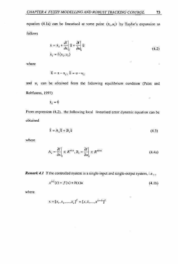
CHAPTER 4 FUZZY MODELLING AND ROBUST TRACKING CONTROL 73
equation (4.1a) can be linearised at some point (x i ,u i ) by Taylor's expansion as
follows
• . af x -= x 1. + —ax x du (4.2)
k i = f(x i ,u i )
where
= x – x i , = u – u i
and u i can be obtained from the following equilibrium condition (Palm and
Rehfusess, 1997)
k i =0
From expression (4.2), the following local linearised error dynamic equation can be
obtained
5.Z = A i R (4.3)
where
af E R"'", B i =
au E Rnxm (4.4a)
Remark 4.1 If the controlled system is a single-input and single-output system, i.e.„
x ( " ) (t) = f (x) + b(x)u (4.1b)
where
T x = [x I x2 • • . , A, n =

0 -
B.=
0 b(x )
(4.4b)
ab + ak
CHAPTER 4 FUZZY MODELLING AND ROBUST TRACKING CONTROL 74
then we have the following linearised system matrices,
0 1 0 00 0
A, =
000 1 a0 a 1 • • a
_ fa ab af a o -+ u — , a l =
ax ax ax x,
which is in a controllable form.
Remark 4.2: If equation (4.3) is in a controllable form, the feedback control law
= (4.5)
can be designed by using conventional linear system theory (Ogata, 1990) so that the
eigenvalues of (A i - B iK i ) are the specified ones. The feedback gain K i can be
designed by using the Ackerman's formula in the case of single-input system as
follows (Ogata, 1990)
K i = (4.6)
where
a(s) = sn + ans' l +...a 2s+
is a desired stable polynomial, and
Q i = [B i AB, /03 i A7 -1 B i ]
4.3 Fuzzy modelling and tracking control of nonlinear systems
4.3.1 Fuzzy modelling and tracking controller design
Many Physical systems are very complex in practice so that it is very difficult to
obtain their rigorous mathematical models. In recent years, fuzzy logic has been

CHAPTER 4 FUZZY MODELLING AND ROBUST TRACKING CONTROL 75
applied to the field of system modelling and control engineering (Takagi and Sugeno,
1985; Wang and Mendel, 1992; Feng et al., 1997) by means of combining human
heuristic reasoning and expert experience. In this section, the fuzzy model is
established by the following fuzzy inference rules which include local linearised
subsystems and feedback controllers.
R': IF x i is AND ... xn is Fril
THEN
5.Z = +
u - u i (4.7)
= 1,2,...,/
where R i denotes the i-th fuzzy inference rule, 1 the number of inference rules,
FJ (j = 1,2,...,n) are fuzzy sets, = x — x d is the tracking error of the system with
desired trajectory x d .
Let it(x) be the normalized membership function of the inferred fuzzy set F i where
n F'= flFJ
and
(x) = 1 i=1
By using a standard fuzzy inference method, that is, using a singleton fuzzifier,
product fuzzy inference and centre-average defuzzifier, the following global tracking
error fuzzy model for the controlled nonlinear system can be obtained,
(4.8)
(4.9)

CHAPTER 4 FUZZY MODELLING AND ROBUST TRACKING CONTROL 76
where
= Ao R +
= u - u d = —KR
A o =E[t i A i B o =D.t i B i i=1 i=1
u d =Ei.t j u i
(4.10)
(4.11)
(4.12)
Remark 4.3: Here, we assume the fuzzy model is globally controllable, that is,
(A0 ,13 0 ) is a controllable pair.
4.3.2 A example of fuzzy modelling and control
Consider the following one-link robotic manipulator
m/ 26 + + mglcos(0) = u (4.13)
with
m = lkg - payload, 1 = lm - length of the link,
g = 9.81m1s 2 - gravitational constant,
d = lkgm 2 /s - damping factor,
u - control variable (kgm 2 /s 2 ).
Assuming we are interested in the dynamics of the system in the range of [-90 0 ,90 0 ],
then the fuzzy model can be obtained by linearising the nonlinear equation (4.13) over
a number of points, such as 0 0 , ± 30 ° , ± 60 ° , ± 90°. The following fuzzy model is
considered
R 1 : IF x l is about - 90° , THEN R= A I R+ B i ll, = u - u l =
R 2 : x i is about - 60 ° , THEN R = A2R. + B 2 11, = U -112 = - K2R
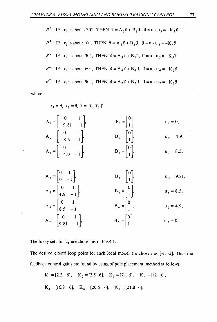
A 5 =
A 6 = [ 0 ii 8.5 —1]
CHAPTER 4 FUZZY MODELLING AND ROBUST TRACKING CONTROL 77
R 3 : IF x i is about - 30°, THEN = A 3 R + B 3 iI, ii = u - u 3 = —K 3 R
R4: IF x 1 is about 0 ° , THEN FC = A 4 R + B411, ii = U - 1.1 4 = -K 4 5-C
R5: IF x 1 is about 30°, THEN5..t" = A 5 it + B 5 1I, II = u - u 5 = —K 5 ,7
R6: IF x 1 is about 60°, THEN R = A 6 R + B 6 i1, il = u - u 6 = —K 6 R
R 7 : IF x i is about 90°, THEN R = A 7 3Z + B 7 11, ii = u - u 7 = —K 7 3Z
where
x, = e, x 2 =0 R = [71 , -72] 7.
u l =0,
11 2 = 4.9,
B3 _
B4 _
B 5
6 B =I
[0] li
,
[i,
01 l 0 [ , 11 01 , li
U 3 = 8.5,
U 4 = 9.81,
U 5 = 8.5,
U 6 = 4.9,
[ 0 ii — [ 0 1 A7 =
9.81 —11 ' 1 U 7 =0.
The fuzzy sets for x 1 are chosen as in Fig.4.1.
The desired closed loop poles for each local model are chosen as [-4, -3]. Thus the
feedback control gains are found by using of pole placement method as follows
6],
I 0 1 i [0 ] B
AI — L— 9.81 —11 i
11
I- 0 11 [01
A2 =[- 8.5 -11 B2 _ li,
r o 1 i A 3 - [- 4.9 - lt
K 1 =[2.2 6], K2 = [3.5 6], K 3 = [7.1 6], K 4 = [12
K5 = [16.9 6], K6 = [20.5 6], K 7 = [21.8 6].

CHAPTER 4 FUZZY MODELLING AND ROBUST TRACKING CONTROL 78
Therefore, the fuzzy control input can be written as
7 7 1.1 = —E[tiKiR +Dotilai (4.14)
i=1 i=1
The control objective in this simulation is to force the one-link robotic manipulator to
follow a desired trajectory which is generated by the following reference model
[id ] = [ 0 1 Ixd 1 + [0111 (4.15)
Id 25 — 10 1 s
where u s is chosen as in Fig.4.2.
In this example, the initial values of x and x d are selected as
[x 1 (0), (0)] = [17.2°, 0], [xd (0), .kd (0)] = [0, 0] .
Fig. 4.3 shows the output tracking using the fuzzy feedback controller. It can be seen
that good tracking performance has been achieved by the proposed fuzzy model. Fig.
4.4 shows the control input.
In order to examine the robustness of the fuzzy model, we use five fuzzy inference
rules instead of seven. If we choose the fuzzy sets as in Fig. 4.5 and the following
fuzzy rules,
R I : IF x i is about - 90 ° , THEN = A I R + B i ii, = u - u 1 =
R 2 : IF
R3: IF x i is about 0°, THEN 5Z = A 3 R + B 3 ii, = U - U 3 = — K 3 R
R4: IF x i is about 45 ° , THEN = A 4 5Z + B 4 11, = u - = —K 4 5Z
R5: IF x i is about 90° , THEN = A 5 5Z + B 5 ii, = u - u 5 = —K 5 R
with

CHAPTER 4 FUZZY MODELLING AND ROBUST TRACKING CONTROL 79
0 1 1 A, = [— 9.81 — lt r 0 '1
A2 — L- 6.94 — It [0 1 1
A3 = L o 0 — lt 0 11
A4 = L694 [6.94 — lt
0 '1 A 5 = [9. 81 — lt
0 B 1 411, u, =0,
rol u 2 =6.94,
1
u 3 =9.81, 1
B 4 =[0 ], u 4 =6.94, 1
0 B 5 =11, U 5 =O.
then the output tracking and fuzzy control input are shown in Fig.4.6 and Fig.4.7,
respectively. It can be seen that the output tracking error is increased in the vicinity of
60 0 in comparison with Fig.4.3. However, if we choose the fuzzy sets as in Fig. 4.8
and the following fuzzy rules,
R1: IF x1 is about - 90 ° , THEN R = A i R + u - u i =—K 1 3
R2: IF x i is about - 60 ° , THEN R = A2 + B 2 , = u - u 2 = —K 2 R
R3: IF xi is about 0 0 , THEN R A 3 R + B 3 1:1, = u - u 3 = —K 3 x
R4: IF x i is about 60 0 , THEN R = A4R + B 4 5, tI = u - u 4 = -- K43C
R5: IF xi is about 90 ° , THEN R = A5R + = u - u 5 =—K 5 R
with
A 1 = 0 1
[-9.81 — 1i'
0 1 A2 = [
— 8.5 —1t
[0 1 A 3 = 0
B i =
B 3 =[]'
-11,
0 [ 1 ],
0
0 1 1
U 1 =0,
U2 = 4 . 9,
U 3 = 9.81,

CHAPTER 4 FUZZY MODELLING AND ROBUST TRACKING CONTROL 80
[ 0 1 A4 =I
8.5 —1I
[ 0 1 A5 = I
9.81 —11
11 4 = 4 . 9,
U7 =0.
then the output tracking and fuzzy control input are shown in Fig.4.9 and Fig.4.10,
respectively. It is clearly shown that the output tracking error is diminished in the
vicinity of 60 0 by comparing with Fig.4.6. Hence, it can be concluded that if the fuzzy
rules are selected appropriately, good tracking performance can then be achieved even
with less fuzzy rules.

Fig. 4.1 Fuzzy sets of xl
40
35
• _ (2 10
5
0 0 2 4 6 8 10 12
Time(s) 14 16 18 20
1
0.9
0.8
0.7
0.6
0.5
0.4
0.3
0.2
0.1
0 —60 0
—80 —20 —40 40 20 80 60
CHAPTER 4 FUZZY MODELLING AND ROBUST TRACKING CONTROL 81
Fig.4.2 The control input of the reference model

CHAPTER 4 FUZZY MODELLING AND ROBUST TRACKING CONTROL 82
Reference vs Actual position of the link
The
outp
ut tr
acki
ng (p
ositi
on in
deg
.)
70
60 -
50 -
40 -
30 -
1
1 I
\
-
-
-
-10 0
._ 2 4 6 8 10 12 14 16 18 20
Time(s)
Fig.4.3 The output tracking of the link, where the solid line represents the desired trajectory.
20
15 -
E 10
0
-50
-
2 4 6 8 10 12 14 16 18 20 Time(s)
Fig 4.4 Fuzzy tracking control input

CHAPTER 4 FUZZY MODELLING AND ROBUST TRACKING CONTROL 83
0.9
0.8
0.7
0.6
0.5
0.4
0.3
0.2
0.1
-80 -60 -40 -20 0 20 40 60 80
Fig.4.5 Fuzzy sets of x i
Reference vs Actual position of the link
The
outp
ut tr
acki
ng (p
ositi
on in
deg
.)
20 -
70
60
50
40
30
I 10-'
t
_
-
_
-
1 1
1 i
1
1
1 1
-10 0
i i i
14 16 18
2 4 6 8 10 12 Time(s)
20
Fig.4.6 The output tracking of the link, where the solid line represents the desired trajectory.

CHAPTER 4 FUZZY MODELLING AND ROBUST TRACKING CONTROL 84
20
15
z 1
o_
o5
2 4 6 8 10 12 14 16 18 20 Time(s)
Fig.4.7 Fuzzy tracking control input
0.9
0.8
0.7
0.6
0.5
0.4
• 0.3
0.2
0.1
-80 -60 -40 -20 0 20 40
60
80
Fig.4.8 Fuzzy sets of x 1

The
outp
ut tr
acki
ng (p
ositi
on in
deg
.)
CHAPTER 4 FUZZY MODELLING AND ROBUST TRACKING CONTROL 85
Reference vs Actual position of the link 70
-10 0
i i i i i
2 4 6 8 10 12 14 16 18 Time(s)
Fig.4.9 The output tracking of the link, where the solid line represents the desired trajectory.
20
20
15
z 1 0
0_ •_
o5
0
-50 2 4 6 8 10 12 14 16 18 20
Time(s)
Fig.4.10 Fuzzy tracking control input

CHAPTER 4 FUZZY MODELLING AND ROBUST TRACKING CONTROL 86
4.4 Robust tracking control with fuzzy nominal model
4.4.1 A robust tracking control scheme
The nonlinear system (4.1) can be expressed by the following error dynamic equation
=(A + AA)R + (B o + AB)ii + Af (4.16)
where AA, AB represent the approximation error and system uncertainties and Af
denotes all the residual errors and disturbances which cannot be covered by AA, AB.
For further analysis, the following assumption is used in what follows (Man and
Palaniswami, 1995)
Assumption 4.1: There exist matrix HE R' and scalar E such that
AA = B o H AB = B O E
° < 0 1-1 1i < Ho 0< j E I <E 0
< 11 61 11 < fo
(4.17)
Remark 4.4: The above assumption is called uncertain matching conditions and have
been used by several researchers (Man and Palaniswami, 1995; Shoureshi et al., 1990;
Tarn et al., 1984). The upper bounds of the system uncertainties, namely
H 0 , Eo and f0 , may be obtained by experiments.
The objective of this section is to develop a robust tracking control scheme which
ensures that the output tracking error 5i asymptotically converges to zero.

CHAPTER 4 FUZZY MODELLING AND ROBUST TRACKING CONTROL 87
The controller design of the nonlinear system in this section is divided into two parts.
First, a nominal feedback controller, as shown in (4.11), is designed based on fuzzy
nominal system model, which guarantees that the tracking error ic of the nominal
system asymptotically converges to zero. Second, a variable structure compensator is
designed based on an uncertain bound to eliminate the effects of the approximation
error and uncertain dynamics so that the tracking error of the closed loop system
with uncertain dynamics asymptotically converges to zero.
The nominal feedback controller for the fuzzy nominal model is derived directly from
(4.11), that is
u 0 =—KR-Fu d (4.18)
where
1 . Ud = E giui (4.19)
Next, we consider the variable structure compensator design for the uncertain system
(4.16). Let the control input in system (4.1) have the following form
u=u 0 +u l (4.20)
where u 0 is the nominal feedback control given in expression (4.18), and u l is a
compensator to deal with the effects of system uncertainties.
Using expression (4.17) and (4.20) in (4.16), the error dynamics of the closed loop
system with uncertainties is written as
= (A 0 —B 0 K)3Z +B 0 (H—EK)R+B 0 (1+E)u 1 +Af (4.21)

CHAPTER 4 FUZZY MODELLING AND ROBUST TRACKING CONTROL 88
In order to use the variable structure theory to design the compensator u i , we define a
switching hyperplane variable as follows
S = CR (4.22)
where C = [c i ,c 2 ,... , c n ] is chosen such that zeros of the polynomial CR =0 are in
the left half of the complex plane, and matrix CI3 0 is non-singular (Man and
Palaniswami, 1995).
For the design of the compensator u 1 and the stability analysis of tracking error
dynamics (4.21), we give the following theorem.
Theorem 4.1: If the nominal feedback control u 0 is given by expression (4.18) and
the compensator u l is designed such that
u l = I O SCB 0 II (SCB 0 )
2 [ SC(A 0 —B 0 K)R +p] S # 0
where
o S = 0 (4.23)
1 P = 1 [ IISC ( A 0 —B oK) R II HIS CB 011(11 011'11 + E011 1(31) — 11 SIIII CIlfo 1 — E 0
(4.24)
then, the tracking error R asymptotically converges to zero as time tends to infinity.
Proof: Defining a Lyapunov function
V = —1 s 2 2
(4.25)
and differentiating v with respect to time, we get

CHAPTER 4 FUZZY MODELLING AND ROBUST TRACKING CONTROL 89
= SS =SCR/6i 0 -B o K)R +B o (H-EK)R + B 0 (1+ E)u i +Af] = -ESC(A 0 -13 0 1()R + SCB 0 (H - EK)R + SCAf + (1- E)p
o K)Rii VEI B DISC(Ao - IISCB 011(1141114 + 1111 1(R 11 ) + Js OCIII1Af 1- E
± [ IISC(A 0 -B 0 1())11 - 0SCB 011 (11 0 E 011 101) HISMCK0 ]
- (1- 11EINSC(A0 -B o K)R 11 - 11SHC11 0. 0 - 11 Af 11 ) -0SCB 0 0[(H o -111-111)114+(E 0 -11E11)11KR11]
<0, forS#0
(4.26)
Expression (4.26) is the sufficient condition for the switching hyperplane variable s to
reach the sliding mode
S = = 0 (4.27)
In the sliding mode, the tracking error Tc asymptotically converges to zero.
Remark 4.5: The robustness property of the proposed control scheme in this section is
obvious. First, the effects of the approximation error and uncertain dynamics can be
eliminated by using the variable structure compensator. Second, the closed loop
system is completely insensitive to uncertainties after the system error dynamics reach
the sliding mode.
Remark 4.6: To eliminate the chattering in the control input, the following boundary
layer compensator (Man and Palaniswami, 1995) can be used in place of expression
(4.23).
I ( 111 = 11=12 [ SC(A 0 - B c,K)R +13 1 IISCB oll< 8 i
8 12
(SCB 0 ) [ SC(A 0 -B 0 K)5Z+ p] IISC13 0 11?_
(4.28)

CHAPTER 4 FUZZY MODELLING AND ROBUST TRACKING CONTROL 90
where 8,> 0.
The above boundary layer compensator can force switching plane variable to move
towards the sliding mode surface and then the control signal can be smoothed inside a
boundary layer. This will achieve optimal trade-off between control bandwidth and
tracking precision. Therefore, the chattering and sensitivity of the controller to system
uncertainties can be eliminated (Man and Palaniswami, 1995).
4.4.2 A simulation example
To illustrate the proposed robust tracking control scheme in this section, a simulation
example is carried out for a one-link robotic manipulator. The dynamic equation of the
one-link robotic manipulator is given by
mI 2 0 + d6 + mgl cos(0) = u (4.29)
with
m = lkg - payload, 1= lm - length of the link,
g = 9.81m1s 2 - gravitational constant,
d = lkgm 2 /s - damping factor,
u - control variable (kgm 2 S 2 ).
Assuming we are interested in the dynamics of the system in the range of [-90° ,90 0 ],
then the fuzzy nominal model can be obtained by linearising the nonlinear equation
(4.29) over a number of points, such as 0° ,±45° ,±90°. The following fuzzy nominal
model has been obtained.

CHAPTER 4 FUZZY MODELLING AND ROBUST TRACKING CONTROL 91
R' : IF x, is about 0° THEN5.".c =A 1 +B 1 ii
R2: IF x, is about - 45°
THEN 5.'(' = A 2 R +
R3: IF x i is about + 45° THEN 5..t' = A 3 5Z +B 3 ii
R4: IF x, is about -90° THEN 3.Z = A 4 R + B 4 1.1
R5: IF x, is about +90°
THEN3-C = A 5 R + B 5 ii
where
x l =0,x 2 = 6, 5-(' =[R,,X* 2 ] T ,u ; = mglcos(0 ; ) -0 1 I
B, — [Cid A ' LO —11'
Lr 0 1 ] [01 1 -6 .94 —11
B2 _
I. 0 1 [Oi l
A3 - L6.94 —11' B3
[ 0 1 1 _ [Oi
] A 4 = B 4
—9.81 —1S [ 0 1 1 _ [Oi
] A 5 = B 5
9.81 —1T
The fuzzy sets for x, are chosen as in Fig.4.11.
The desired closed loop poles for each local model are chosen as [-4, -3]. Thus the
feedback control gains are found by using of pole placement method as follows

CHAPTER 4 FUZZY MODELLING AND ROBUST TRACKING CONTROL 92
=[12 6], K 2 = [5.1 6], K 3 = [18.9 6], K 4 = [2.2 6], K 5 =[21.8 6].
The control objective in this simulation is to force the one-link robotic manipulator to
follow a desired trajectory which is generated by the following reference model
[i d [ 0 — 25
1 1[X d 10 i d
[Olu 1 s
(4.30)
where u s is chosen as in Fig. 4.12.
In this example, the initial values of x and x d are selected as
[x 1 (0), x (0)] = [17.2° ,0], [x d (0), d (0)] = [0,0] .
Sliding mode is prescribed as
S = [10,1][_ 1 1. X 2
Uncertain bounds are selected as
E 0 = 0.1, H o = 2, fo = 1.
Fig. 4.13 shows the output tracking using only a fuzzy nominal feedback controller. It
can be seen that due to large system uncertainties, the output cannot track the desired
trajectory closely. Fig. 4.14 shows the output tracking and control input using a fuzzy
nominal feedback controller with a variable structure compensator. Obviously, the
effects of the system uncertainties are eliminated and a good tracking performance is
achieved. But there exists chattering in the control input. Fig. 4.15 shows good
performance of the closed loop system in which a fuzzy nominal feedback controller
with a boundary layer compensator is used to eliminate control chattering.

CHAPTER 4 FUZZY MODELLING AND ROBUST TRACKING CONTROL 93
4.5 Concluding remarks
A robust tracking control scheme has been proposed in this chapter for a class of
nonlinear systems. The main contribution of this scheme is that a nominal system
model for a nonlinear system is established by fuzzy synthesis of a set of linearised
local subsystems, where the conventional linear feedback control technique is used to
design a feedback controller for the fuzzy nominal system. A variable structure
compensator is then designed to eliminate the effects of the approximation error and
system uncertainties. Strong robustness with respect to large system uncertainties and
asymptotic convergence of the output tracking error are obtained. A simulation
example has been given to support the proposed control scheme.

40 60 80 100
1
0.9
0.8
0.7
0
g 0.4
0.3
0.2
0.1
0 -100 -80 -60 -40 -20 0 20
Position (deg)
CHAPTER 4 FUZZY MODELLING AND ROBUST TRACKING CONTROL 94
Fig.4.11 Fuzzy sets of state x 1
100
90
80
70
ED_ ) 60
a) _c 20
10
oo
2 3 4 5 6
7
8
9
10 Time(s)
Fig. 4.12 The input signal u s of the reference model

— I
-
CHAPTER 4 FUZZY MODELLING AND ROBUST TRACKING CONTROL 95
Nom
ina l
con
trol i
nput
Reference vs Actual position of the link
-50 1 2 3 4 5 6 7 8 9 10
Time(s)
Fig.4.13-a The output tracking of the link using a fuzzy nominal feedback controller. Solid line represents the desired trajectory
25
20 -
15 -
10 -
45
40
_35
Q)
-° 30
0 ti 25 0 0_ 220 cy;
15 o_ 0 10 a) _c
5
0
-100 1 2 3 4 5 6 7 8 9 10
Time(s)
Fig. 4.13-b Nominal feedback control input

0 co
CHAPTER 4 FUZZY MODELLING AND ROBUST TRACKING CONTROL 96
45
40
35 o) a)
7.3 30 •S 0 E 25 0 0_
F20
5 - 1
Reference vs Actual position of the link
1 2 3 4 5 6 Time(s)
7 8 9 10
Fig. 4.14-a The output tracking with variable structure compensator
50
40
30 -
8 i o -
—10
—20 0
■ ■ 5 6 7
Time(s) 1 2 3 4 9 10
Fig. 4.14-b Control input with compensator

CHAPTER 4 FUZZY MODELLING AND ROBUST TRACKING CONTROL 97
45
40 -
35 -
.1 25- 0
E.20 -
co 15 4
0_ 5 0 10
5
Reference vs Actual position of the link
1 2 3 4 5 6 Time(s)
7 8 9 10
Fig. 4.15-a The output tracking using boundary layer compensator (6, = 0.04).
40
30
20
5 0_
• 10
0
- 10
II -20 0 1 2 3 4 5 6
Time(s) 7 a 9 10
Fig. 4.15-b Control input with boundary layer compensator ( 6, = 0.04).

CHAPTER 5 FUZZY SLIDING MODE CONTROL 98
Chapter 5
Fuzzy Sliding Mode Control
5.1 Introduction
Fuzzy logic technique based on approximate reasoning has been widely used for the
design of control systems (Mamdani and Assilian, 1974; Tagalci and Sugeno, 1985;
Cao et al., 1996). The early fuzzy control algorithms proposed by Mamdani et al. have
the following characteristics (Yager and Filev, 1994): (i) The detailed mathematical
description of the controlled system is not required, (ii) the human experience and
understanding about the system are used to design a fuzzy controller which allows us
to implement heuristic strategies, which are defined by linguistically described
statements, to formulate the control algorithm.
In order to improve the performance of fuzzy control systems, the fuzzy control
algorithms with the Mamdani model have been further investigated and developed in
recent years. It is shown that (Yager and Filev, 1994), if the structure of the fuzzy

CHAPTER 5 FUZZY SLIDING MODE CONTROL 99
control networks can be identified and the membership functions of the fuzzy sets can
be estimated by the use of some optimisation techniques, a satisfactory tracking
performance of the closed loop fuzzy systems can be obtained.
In this chapter, Lyapunov stability theory and fuzzy logic technique are combined
together to design sliding mode controller. It is shown that a sliding mode is first
designed to describe the desired system dynamics for the controlled system. A set of
fuzzy rules are then used to adjust the parameters of the controller based on the
Lyapunov function and its derivative. The sliding mode controllers with fuzzy tuning
algorithm show the advantage of reducing the chattering of the control signals, which
makes the fuzzy sliding mode control more practical. A simulation example is given in
support of the proposed control scheme.
The chapter is organised as follows. In section 5.2, a class of nonlinear systems to be
considered, Lyapunov function and the sliding mode controllers are formulated. In
section 5.3, the fuzzy rules used to adjust the parameters of the controller are
described in detail. In section 5.4, a simulation for a one-link rigid robotic manipulator
is performed in support of the proposed control scheme. Section 5.5 gives concluding
remarks.
5.2 Sliding mode control of nonlinear systems
In this paper, we focus on the design of sliding mode controllers for a class of
nonlinear systems whose dynamic equations can be expressed in the following form
(Gao and Hung, 1993):

CHAPTER 5 FUZZY SLIDING MODE CONTROL 100
= A(x)+ B(x)u (5.1)
where dim-x = n, dim-u = m, n > m, and A(x) and B(x) are of appropriate
dimensions. The switching surface is defined by
s(x)=c T x =0 (5.2)
where c T = [c 1 c 2 • • • c n ] is chosen such that the zeros of the polynomial c T X =0
are in the left half-plane and c T B(x) O. Eqn. (5.2) represents a desired system
dynamics with a lower order than the given plant. The sliding mode controller u is
designed such that any state x outside the switching surface is driven to reach the
surface. On the switching surface, the sliding mode takes place, following the desired
system dynamics.
Theorem 5.1: If the control law is designed as follows
U = T B(X)}-1 A(x) + Qsgn(s) + Kh(s)] (5.3)
where
Q = diag[q , • • • , q ], q > 0
sgn(s) = [sgn(s ), • • • , sgn(s )] T
K = diag[k i ,• • • , k m ], k, > 0
h(s)= [h i (s i ),•••, h. (s. )] T
Si h i (s ) > 0, h (0) = 0
then the system state x reaches origin as time tends to infinity.

CHAPTER 5 FUZZY SLIDING MODE CONTROL 101
Proof. Consider the following Lyapunov function
1 T V = 2
(5.4)
The derivative of V is
= sT§
T T• =S C X
=S T C T [A(x)+ B(x)u]
= s T C T [A(x)— B(x){c T Br' [c T A(x) + Qsgn(s) + Kh(s)]]
= —s T [Qsgn(s) + Kh(s)] <0 s # 0 QED.
(5.5)
From (5.5), we have the following reaching law,
S = —Qsgn(s) — Kh(s) (5.6)
It is clearly known that, if Q is too small, the reaching time will be too long. On the
other hand, a large Q will cause severe chattering. In next section, a fuzzy tuning
algorithm for Q is introduced to achieve a better trade-off between the settling time
and chattering phenomena.
5.3 Fuzzy tuning of the sliding mode controller
The Mamdani's fuzzy inference model (Mamdani and Assilian, 1974) is used to adjust
the controller's parameter matrix Q. The Lyapunov function defined in (5.4) can be
considered as the distance between the desired and actual states. The control objective

CHAPTER 5 FUZZY SLIDING MODE CONTROL 102
is that the distance should be decreased as soon as possible. We divide the Lyapunov
2 function -s (V) into three fuzzy subsets, such as 'big', 'medium' and 'small'. The 2 I
convergent rate or the derivative of Lyapunov function s i S (V) is divided as the
fuzzy subsets 'positive', 'zero' and 'negative'. The fuzzy control system consists of
two linguistic input variables V and V and one linguistic output variable Q. The two
fuzzy input variables are defined as follows
V={B, M, S} (5.7)
V={P, Z, NI (5.8)
where B = big, M = medium, S = small, P = positive, Z = zero, N = negtive. Fuzzy
output variable Q is defined as follows
Q={B, MB, M, MS, S} (5.9)
where MB = medium big, MS = medium small. The input-output relation of the fuzzy
controller with fuzzy variables (5.7), (5.8) and (5.9) is written by
V, V —> Q (5.10)
The fuzzy tuning algorithm for Q is described in fuzzy rules as follows and also
represented in "look-up" Table 5.1.
1. If (V is B) and ( V is P) then (Q is B)

CHAPTER 5 FUZZY SLIDING MODE CONTROL 103
2. If (V is B) and ( V is Z) then (Q is MB)
3. If (V is B) and ( V is N) then (Q is M)
4. If (V is M) and ( V is P) then (Q is MB)
5. If (V is M) and ( V is Z) then (Q is M)
6. If (V is M) and ( V is N) then (Q is MS)
7. If (V is S) and ( is P) then (Q is M)
8. If (V is S) and ( V is Z) then (Q is MS)
9. If (V is S) and ( V is N) then (Q is S)
Remark 5.1: The above fuzzy rules carry the control principle: when V is 'big' and
V is 'positive' (i.e., V is increasing), then chose 'big' control input Q to force the
system state to converge to the desired state faster; when V is 'small' and V is•
'negative' (i.e., V is decreasing), then chose 'small' control input Q to decrease
control chattering.
Q
V
P z N
V
aci cn
B
MB
M
MB
M
MS
M
MS
s
Table 5.1. Fuzzy inference rules table

$ i
0.8
0.2
o
Isn
CHAPTER 5 FUZZY SLIDING MODE CONTROL 104
The membership functions for fuzzy variables V, V, and Q with normalised universe
of discourses are chosen as in Fig. 5.1 (a)-(c). The fuzzy inference surface is shown in
Fig. 5.1 (d).
0 0.1 0.2 0.3 0.4 0.5 0.6
0.7
0.8
0.9
i Lyapunov Junction
Fig. 5.1 (a) Fuzzy subsets of V

0.8 -0.8 -0.6 -0.4 -0.2 0 0.2 0.4
0.6 Change_rate_of_Lyapunovf unction
Fig. 5.1 (b) Fuzzy subsets of
MB
1 0 0.1 0.2 0.3 0.4 0.5 0.6
0.7
0.8
0.9 Control_parameter_Q
1
0.8
0.2
0
1
0.8
0.2
0
1
CHAPTER 5 FUZZY SLIDING MODE CONTROL 105
Fig. 5.1 (c) Fuzzy subsets of Q

CHAPTER 5 FUZZY SLIDING MODE CONTROL 106
V_dot V
Fig. 5.1 (d) Surface of Q (V, V)
5.4 An illustrative example
To illustrate the proposed fuzzy tuning sliding mode control scheme in this chapter, a
simulation example is carried out for a one-link rigid robotic manipulator. The
dynamic equation of motion of the manipulator is given by
m1 26 + do + mglcos(0) = u + u d (5.11)
with m = lkg,1= lm , g = 9.81m/s 2 , d = lkgm 2 /s , and Li d = 0.3sin(10t) is the
external disturbance.
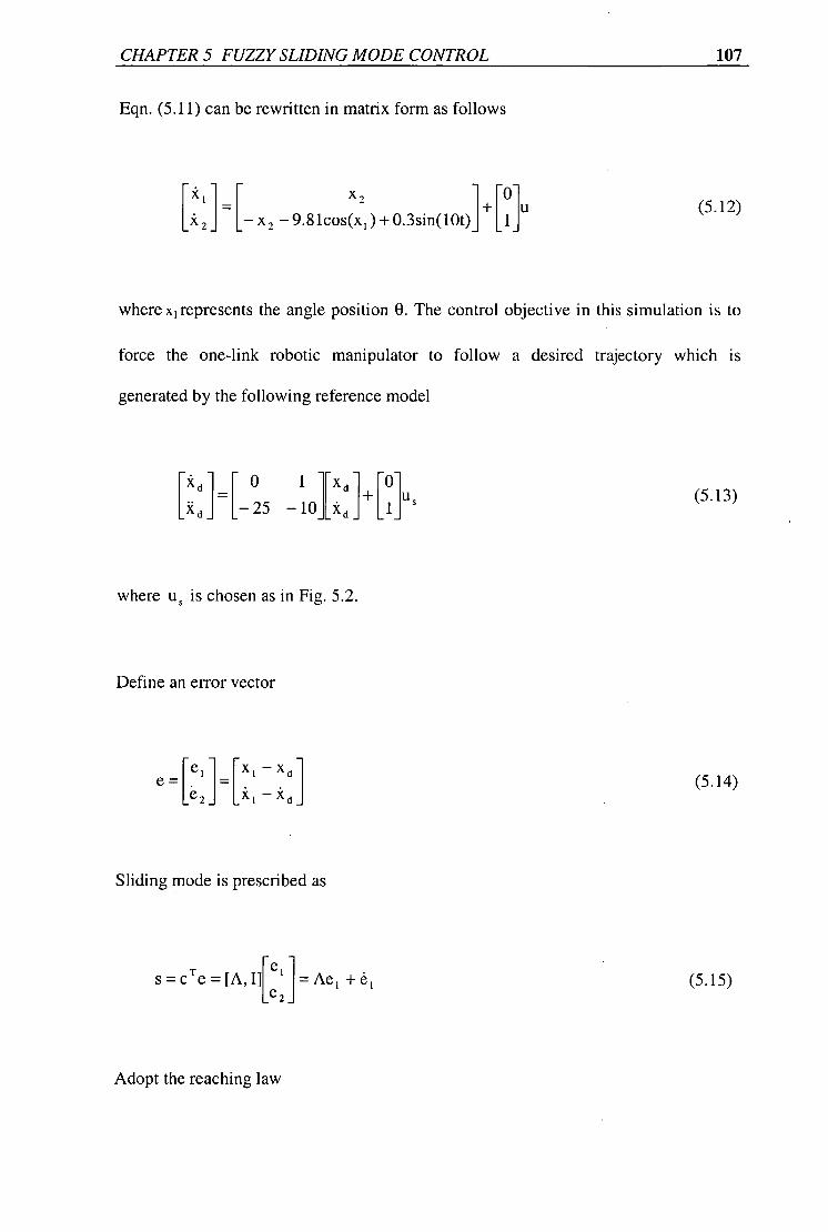
CHAPTER 5 FUZZY SLIDING MODE CONTROL 107
Eqn. (5.11) can be rewritten in matrix form as follows
[X X2 1 +u [01
5( 2 — x 2 —9.81cos(x 1 )+0.3sin(10t) 1 (5.12)
where x i represents the angle position 0. The control objective in
force the one-link robotic manipulator to follow a desired
generated by the following reference model
this simulation is to
trajectory which is
r kdi j 0 1 irx di±r0iu L 3, di L-25 _mikdi [
j us (5.13)
where u s is chosen as in Fig. 5.2.
Define an error vector
e ie 1 1 . [x —x d ]
—kd (5.14)
Sliding mode is prescribed as
e i s = c T e = [A, If 1= Ae i + é 1 e 2
(5.15)
Adopt the reaching law

CHAPTER 5 FUZZY SLIDING MODE CONTROL 108
§ = —Q sgn(s) (5.16)
Taking the time derivative of (5.14) gives
.i• = Ae l — k d — x 2 — 9.81cos(x 1 )+ 0.3sin(10t) + u (5.17)
Equating (5.16) and (5.17) and solving for the control u yields
u = —Q sgn(s) — Ae, + k d + X 2 ± 9.81cos(x 1 ) - 0.3sin(10t) (5.18)
Fig. 5.3 shows the output tracking using the conventional sliding mode controller
(5.18) with Q=5 and A=6, which is shown in Fig. 5.4. Fig. 5.5 shows the output
tracking using a sliding mode controller (5.18) with fuzzy tuning for Q, the control
input is shown in Fig. 5.6. The scaling factor for fuzzy variables s 2 ,s and Q are
chosen as 1, 6 and 5, respectively. It can be seen that the control chattering is greatly
reduced with fuzzy tuning.

CHAPTER 5 FUZZY SLIDING MODE CONTROL 109
30
25
0
a) 0 20 EL)
2 a)
15
cr)
.5 10 c). • _
5
00 5 10 15 20 25
Time(s)
Fig. 5.2 The input signal of the reference model
Reference vs Actual position of the link 50
40
The
outp
u t tr
acki
ng (p
ositi
on in
deg
. )
30
20
lo
-1 0 5 10 15 20 25 30 35
40
Time(s)
30 35 40
Fig. 5.3 The output tracking with conventional sliding mode controller

CHAPTER 5 FUZZY SLIDING MODE CONTROL
40
30 -
110
■ 5 10 15 20 25
Time(s) 30 40 35
Fig.5. 4 The sliding mode control input without fuzzy tuning
Reference vs Actual position of the link 50
40
30
20
1 0 T
0
I i ■ 5 10 15 20 25 30 35
Time(s)
Fig.5. 5 The output tracking with fuzzy tuning
The o
utp
ut t
rac k
ing
(pos
ition
in d
eg. )
40

CHAPTER 5 FUZZY SLIDING MODE CONTROL 111
30
25
20
15
cl 10 •_ \+0++0+0404444S+4+00
0
-10 -
-150 5 10 15
■ 20 25 30 35 40
Time(s)
4,4-14+++4++i+ ■44++4++++++o++++
44+0+44444044044044+44
Fig. 5.6 The control input with fuzzy tuning sliding mode controller
5.5 Concluding remarks
In this chapter, Lyapunov stability theory and fuzzy logic technique are combined
together to design sliding mode control systems. It is shown that a sliding mode is
first designed to describe the desired system dynamics for the controlled system. A set
of fuzzy rules are then used to adjust the parameters of the controller based on the
Lyapunov function and its derivative. The sliding mode controllers with fuzzy tuning
algorithm show the advantage of reducing the chattering of the control signals,
compared with the conventional sliding mode controllers. A simulation example using
fuzzy sliding mode control for a one link robotic manipulator is given in support of the
proposed control scheme.

CHAPTER 6 ROBUST CONTINUOUS SLIDING MODE CONTROL 112
Chapter 6
Robust Continuous Sliding Mode Control
6.1 Introduction
Sliding mode control (SMC), based on the theory of variable structure systems, first
proposed by Emelyanov in 1967, has attracted a lot of research on control systems for
the last two decades. Sliding mode control is a robust control technique that has been
successfully used for the control of linear and nonlinear systems. In order to design
sliding mode control systems, a switching surface or a sliding mode is defined first,
then a sliding mode controller is designed to drive the system state variables to the
switching surface. If the system state is above or below the switching surface, then the .
controller will drive the system state back to the surface. Once the system state reaches
the switching surface, the system state will slide along the switching surface, and the
dynamics of the controlled system is pre-determined by the sliding mode parameters
and remains insensitive to variations of system parameters and external disturbances.

CHAPTER 6 ROBUST CONTINUOUS SLIDING MODE CONTROL 113
The main drawback of sliding mode control is the associated undesirable chattering
problem. It not only increases wear of the final control element but also excites high
frequency unmodelled plant dynamics (Slotine and Sastry, 1983). To reduce this
unwanted control chattering, Slotine and Sastry (1983) proposed a 'boundary layer'
approach which approximates the ideal relay characteristics used by sliding mode
control by linear saturated amplifier characteristics. This boundary layer sliding mode
control only guarantees that the state will converge to a band (boundary layer)
centered on the sliding mode. It provides no guarantee that the state will converge
exactly to the sliding mode, although the state can be brought arbitrarily close to the
sliding mode by narrowing the boundary layer at the cost of higher control authority.
As an alternative, Zhou and Fisher (1992) proposed a continuous approach using the
concept of boundary layer equivalence. The main disadvantage of this technique is
that it tends to produce conservative designs. Because their control law is equivalent to
a cubic feedback control, therefore, the control input may be very large and exceeds
control element's physical limits.
Recently, Ha and Negnevitsky (1996) introduced a fuzzy tuning sliding mode control,
it is shown that the control performance can be improved by fuzzy tuning.
In this chapter, we present a robust continuous sliding mode control scheme based on
Lyapunov stability theory. The proposed controller consists of three components:
equivalent control, continuous reaching mode control and robust control. It retains the
positive properties of sliding mode control but without the disadvantage of control

CHAPTER 6 ROBUST CONTINUOUS SLIDING MODE CONTROL 114
chattering. As an example, the proposed control scheme is applied to the design of a
robust tracking controller for a one-link robotic manipulator.
6.2 A robust continuous sliding mode control
Consider a linearised dynamic system described by
= (A + AA)x + (B + AB)u (6.1)
where x E R" is the state vector, u E R is the control signal, AE IV" and BE R
are the nominal system matrices and in controllable form, AA and AB represent
uncertainties. The following matching condition is used for further discussion (Man
and Palaniswami, 1995):
AA = BH AB = BE (6.2)
with
0 <114 1 <H0 O<IEI<E0 <1
Remark 6.1: Because (A, B) is in controllable form, therefore E is a scalar.
Sliding variable is defined by,

CHAPTER 6 ROBUST CONTINUOUS SLIDING MODE CONTROL 115
s = cTx (6.3)
where C T 4c, c 2 . • • c 11 ] is chosen such that the zeros of the polynomial
C T X = 0 are in the left half-plane and C T B # 0.
A equivalent control is given by S =0 or:
C T X =C T (Ax + Bu e0= 0 (6.4)
that is
u eg = —K eq x = —(C T B) -1 C T Ax (6.5)
A continuous reaching mode controller can be designed by following reaching law:
= —Qerf() (6.6)
where Q is a positive reaching law parameter, 5 is a positive number, and erf(x) is a
standard error function. The continuous sliding mode controller can be easily derived
as
u, = —(C T By' Qerq-) (6.7)

CHAPTER 6 ROBUST CONTINUOUS SLIDING MODE CONTROL 116
In order to deal with system uncertainties, a robust controller is designed as folllows:
SC T B 1 (1-1 0 114 + E 0 1lK eq 4)
Hence, the robust continuous sliding mode controller is represented by
u = u eq + u c + u r (6.9)
Theorem 6.1: If the controller is given by (6.9), then the system state x reaches origin
as time tends to infinity.
Proof: Define a Lyapunov function
Then
1 V = —S 2 2
V = SS
= SCT k
= SCT [(A + AA)x + (B + AB)u]
= SCT [Ax + BHx + B(1+ E)u]
= SC T Ax + SC T BHx
(6.10)
+ (1+ E)[—SC T Ax — SQerf(T5S ) —1SCTBI 1 —
1 Eo (14 011 x 11 + EollKeci 4)1
< —ESC T Ax + SCTBHx —SCTI311 1 1E1 (Ho Oxli + E0K eq 11 x 11 ) D 1— E — o
1EE 1 (H 0 114 ± E 0 11K eq x11) = —ESC T BK eq x + SC T BHx — ISCT BO 11--
<0 if S#0
U r = II SC T B ll 1 - E 0 (6.8)
QED

CHAPTER 6 ROBUST CONTINUOUS SLIDING MODE CONTROL 117
6.3 A simulation example
To illustrate the proposed robust continuous sliding mode control scheme in this
chapter, a simulation example is carried out for a one-link robotic manipulator. The
dynamic equation of the one-link robotic manipulator is given by
m1 2 6 + dO + mgl cos(0) = u (6.11)
with
m = lkg - payload, 1= lm - length of the link,
g = 9.81m1s 2 - gravitational constant,
d = lkgm 2 /s - damping factor, u - control variable (kgm 2 / s 2 ).
In Chapter 4, a fuzzy modelling of a nonlinear system is obtained by linearising
procedures and the following fuzzy inference rules,
R': IF x is F: AND ... x is F i;
THEN
= + B i ll
ii=u-u i (6.12)
i = 1,2,...,/
where R i denotes the i-th fuzzy inference rule, / the number of inference rules,
(j = 1,2,...,n) are fuzzy sets, = x — x d is the tracking error of the system with
ro _ _ desired trajectory x d , and x — [ xx 2
1— 0

CHAPTER 6 ROBUST CONTINUOUS SLIDING MODE CONTROL 118
Let [t i (x) be the normalized membership function of the inferred fuzzy set F i where
and
n
F'=flFj i=1
= 1
(6.13)
(6.14)
By using a standard fuzzy inference method, that is, using a singleton fuzzifier,
product fuzzy inference and centre-average defuzzifier, the following global tracking
error fuzzy model for the controlled nonlinear system can be obtained,
3:C = (A + AA)R + (B + AB)i:i (6.15)
(6.16)
where
A =Ept i A ; B =Ett i B i u, =E gi u ;
AA and AB represent system uncertaities.
Assuming we are interested in the dynamics of the system in the range of [-90 0 ,90 0 ,
then the fuzzy model can be obtained by linearising the nonlinear equation (6.11) over
a number of points, such as 0° , ± 60°, ± 900. The following fuzzy model has been
obtained.

CHAPTER 6 ROBUST CONTINUOUS SLIDING MODE CONTROL 119
R : IF x is about -90°,
THEN X. = = u-u,
R 2 : IF x, is about -60°,
THEN 5Z = A 2 R + = u - u 2
R 3 : IF x, is about 00 ,
THEN R. = A 3 R+B 3 11, i1=u-u 3
R 4 : IF x, is about 60 0 ,
THEN R=A 4 R+B 4 i.i, i= u-u,
R 5 : IF x, is about 90°,
THEN 3Z = A 5 R+B 5 11, ii=u-u 5
with
0 1 A=I ,
—9.81 — 11'
0 1 A2 = [ —8.5 — 11 '
] 1 1 A 3 = [0 0 - il
131 =[j'
B 2 =
B 3 =
1
1 r
1 , ri
'
'
u '
u 2
U 3
= 0,
=4.9,
= 9.81 1 [ 8.5 —0 ii r0i A 4 = 134 =
[] , u, =4.9,
[ 0 9.81 —1'
1 A 5 = B 5 = [1, U 5 = 0.
1 1
Fig. 6.1 shows the membership functions. Choosing Q =10,8 = 0.3, H o = 2, the
simulation results are shown in Fig. 6.2 —6.8. Fig. 6.2 shows the output tracking.
Fig.6.3 shows the control signal, it is observed that no chattering occurred with the
proposed robust control scheme. Fig. 6.4 shows the tracking error. Fig. 6.5-6.7 show
the three control components: equivalent control, continuous reaching mode control,
and robust control, respectively. Fig. 6.8 shows the phase portrait.

CHAPTER 6 ROBUST CONTINUOUS SLIDING MODE CONTROL 120
Choosing Q = 10, 8 = 1, H o = 2, the simulation results are shown in Fig. 6.9 —6.15.
Fig. 6.9 shows the output tracking. Fig.6.10 shows the control signal, it is observed
that no chattering occurred with the proposed robust control scheme. Fig. 6.11 shows
the tracking error. Fig. 6.12-6.14 show the three control components: equivalent
control, continuous reaching mode control, and robust control, respectively. Fig. 6.15
shows the phase portrait.
Choosing Q = 10, H o = 2, and using discontinuous control u d = —Qsgn(S) instead of
u c , then the simulation results are shown in Fig. 6.16 —6.22. Fig. 6.16 shows the
output tracking. Fig.6.17 shows the control signal, it is observed that severe chattering
occurred with the discontinuous control scheme. Fig. 6.18 shows the tracking error.
Fig. 6.19-6.21 show the three control components: equivalent control, discontinuous
control, and robust control, respectively. Fig. 6.22 shows the phase portrait.
6.4 Concluding remarks
In this chapter we developed a robust continuous sliding mode control scheme for
linear systems with uncertainties. The controller consists of three components:
equivalent control, continuous reaching mode control and robust control. It retains the
positive properties of sliding mode control but without the disadvantage of control
chattering. The proposed control scheme has been applied to the tracking control of a
one-link robotic manipulator by fuzzy modelling of the nonlinear system.

CHAPTER 6 ROBUST CONTINUOUS SLIDING MODE CONTROL 121
T he
outp
ut tr
acki
ng (
deg.
)
1
0.9
0.8
0.7 c o "ti 0.6 C m a 1E 0.5 12
23
2
0.3
0.2
0.1
0 -80
60
50 -
40
3
20
10
0
-10 0
-60 -40 -20 0 20
40 Position (deg)
Fig.6.1 Membership functions for positions
60
80
_
_
-
-
_
2 4 6 8 10 12
14
16
18
20 Time(s)
Reference vs Actual position of the link
Fig.6.2 Output tracking performance (8 = 0.3)

122 CHAPTER 6 ROBUST CONTINUOUS SLIDING MODE CONTROL
25
20 -
15
Con
trol i
nput
(N
m)
10
-10
0
2 4 6 8 10 12 14 16 18 20 Time(s)
Fig.6.3 Control input (8 = 0.3)
20
15
0
2 4 6 8 10 12 14 16 18 20 Time(s)
Fig.6.4 Tracking error (8 = 0.3)
-50

CHAPTER 6 ROBUST CONTINUOUS SLIDING MODE CONTROL 123
20
8
16
14-
12 2
-.....
a) z 8 -
-
-
-
_
-
-
-
_
_
, 2 4 6 8 10 12 14 16 18 20
Time(s)
Fig. 6.5 Control component u e (8 = 0.3)
10
-E.' z C.) =
- -
- -
- _
- -
-10 0 2 4 6 8 10 12 14 16 18
Time(s)
Fig. 6.6 Control component u c (8 = 0.3)
20

CHAPTER 6 ROBUST CONTINUOUS SLIDING MODE CONTROL 124
2.5
1.5 -
0.5
-0.5 -
- 1.5
- 2.50
, , , ,
2 4 6 8 10 12 14 16 Time(s)
Fig. 6.7 Control component u,. (8 = 0.3)
18 20
50
0
o) C *•a a -50
"5 a)
'fa= • -100 a) -a
- 150
- 200
-5
5 10
15
20 Tracking error
Fig. 6.8 Phase portrait (8 = 0.3)

CHAPTER 6 ROBUST CONTINUOUS SLIDING MODE CONTROL 125
Reference vs Actual position of the link 70
60
50
The
outp
ut tr
acki
ng (
deg.
)
40
30
20
10
0 0
2 4 6 8 10 12 14 16 Time(s)
Fig. 6.9 Output tracking (8 =1)
18 20
_
25
20
15
-
Con
trol i
nput
(N
m) 10- 0-
L
-
-10 -
-150
■I
2 4 6 8 10 12 14 16 18 20 Time(s)
Fig. 6.10 Control input (8 = 1)

CHAPTER 6 ROBUST CONTINUOUS SLIDING MODE CONTROL 126
20
15
-50 2 4 6 8 10 12 14 16 18 20
Time(s)
Fig. 6.11 Tracking error (8 = 1)
20
15
1 0
a)
5
2 4 6 8 10 12 14 16 18 Time(s)
Fig. 6.12 Control component u e (8 = 1)
20

CHAPTER 6 ROBUST CONTINUOUS SLIDING MODE CONTROL 127
10
-
- _
-
_
-E - z 0
- -
-
-
_
- 10 0 2 4 6 8 10 12
Time(s)
_
-
-
-
14 16 18 20
Fig. 6.13 Control component u c (8 = 1)
1.5
-
0.5 -
"E' '5
_
-1.5
-
-
-
- 2.50
2 4 6 8 10 12 Time(s)
14 16 18 20
Fig. 6.14 Control component U r (8 = 1

CHAPTER 6 ROBUST CONTINUOUS SLIDING MODE CONTROL 128
50
0
15 20 0
5 10 Tracking error
.Fig. 6.15 Phase portrait (5 = 1)
Reference vs Actual position of the link 70
60
50
-
- ■I
The
outp
ut tr
acki
ng (
deg.
)
40
30
-
-
20 -
1 0 ! i
1 ‘
0 _,.
—10 0 2 4 6 8 10 12
Time(s) 14 16 18 20
Fig. 6.16 Output tracking (sgn(s))

11111111111111 CHAPTER 6 ROBUST CONTINUOUS SLIDING MODE CONTROL 129
35
30
25
20
15
10
5
0
-5
- 10
- 15 0 2 4 6 8 10 12
14
16
18
20 Time(s)
Fig. 6.17 Control input (sgn(s))
20
15
0
- 50
2 4 6 8 10 12 14 16 18 20 Time(s)
Fig. 6.18 Tracking error (sgn(s))
Con
trol i
nput
(N
m)

14
12
'...- -10
G) 7
8
--E - z -0 m
CHAPTER 6 ROBUST CONTINUOUS SLIDING MODE CONTROL 130
20
18
16
■ ,
2 4 6 8 10 12 14 16 18 Time(s)
Fig. 6.19 Control component u e (sgn(s))
-
-
-
-
20
2 4 6 8 10 12
14 Time(s)
Fig. 6.20 Control component u d (sgn(s))
16
18
20

-200 15 5 10
Tracking error 20 -5
50
-150
CHAPTER 6 ROBUST CONTINUOUS SLIDING MODE CONTROL 131
2.5
1.5
- 1.5
- 2.5 , ■
2 4 6 8 10 12 Time(s)
14 16 18 20
Fig. 6.21 Control component Ur (sgn(s))
Fig. 6.22 Phase portrait (sgn(s))

CHAPTER 7 FUZZY ADAPTIVE SLIDING MODE CONTROL 132
Chapter 7
Fuzzy Adaptive Sliding Mode Control
7.1 Introduction
Adaptive control of mechanical manipulators has been studied extensively by many
researchers using various methodologies (Craig and Sastry, 1986; Slotine and Sastry,
1984; Balestrino et al., 1979; Young, 1978), such as hyperstability theory, Lyapunov
stability method, self-tuning regulator control and sliding mode control (SMC).
Among the various methodologies, the SMC demonstrates its good robustness and low
computational cost. SMC is a discontinuous feedback control that switches the system
control structure during the evolution of the system state so that the system states
remain in a prescribed subspace. A SMC controller for robot manipulators suggests
that each manipulator link matches a first order sliding motion such that when the
system state reaches the sliding mode, it chatters along the sliding mode and exhibits
sensitivity to the system parameter variations and external disturbances (Slotine and
Li, 1987).

CHAPTER 7 FUZZY ADAPTIVE SLIDING MODE CONTROL 133
One of the well known results in SMC design for trajectory tracking of robotic
manipulators was obtained by Slotine and Li (1987, 1991). Their adaptive SMC is
based on the linear parametrization approach for the robotic systems which do not
involve any uncertainties and disturbances. The validity of the control algorithm is
based on the assumption that the system parameters must be constant and the desired
trajectory should be sufficiently "rich" to guarantee parameter convergence. To
overcome the robustness problem of Slotine and Li's controller, Su and Leung (Su and
Leung, 1993) have proposed a modification that employs the bound estimation
algorithms in the controller to give rise to a robust adaptive SMC controller without a
priori knowledge of upper bounds of the system parameters. This controller is able to
handle large and time varying variations in the parameters. However, the problem is
that their control torques designed incur very large chattering which is not desirable in
practice, especially in mechanical systems.
In chapter 5, a fuzzy tuning algorithm was employed for conventional sliding mode
control to diminish undesired control chattering. In this chapter, a fuzzy tuning
adaptive sliding mode control is proposed for trajectory tracking of rigid robotic
manipulators with uncertainties to achieve robustness as well as desired qualities such
as minimal chattering and small control torques.
This chapter is organised as follows: In Section 7.2, a fuzzy tuning adaptive sliding
mode controller is presented. Section 7.3 describes the experimental results for
confirmation of the theoretical results. Section 7.4 gives concluding remarks.

CHAPTER 7 FUZZY ADAPTIVE SLIDING MODE CONTROL 134
7.2 Robust adaptive SMC with fuzzy tuning
Consider the dynamics of the n-joint robotic manipulators represented by the
following second order nonlinear vector differential equation
H(q)4+ C(q,q)q+ g(q) = r(t)+E(t) (7.1)
where q(t) is the nxl vector of joint angular positions, H(q) is the nxn symmetric
positive definite inertia matrix, C(q,q)q is the nxl vector containing Coriolis,
centrifugal forces, g(q) represents the derivation of the manipulators potential energy,
r(t) is the nxl vector of applied joint torques which are actually control inputs, and
E(t) is the nxl bounded input disturbances vector.
We assume that the robotic manipulators have uncertainties, i.e.
H = Ho + All (7.2)
C= Co + AC (7.3)
g = go + Ag (7.4)
where H0 ,CO3 go are the nominal part and AH, AC, Ag are the uncertain part. The
uncertain components represent bounded small possible time varying, unmodelled
dynamics or load changes. Substituting the expressions (7.2)-(7.4) into the dynamics
(7.1) gives rise to
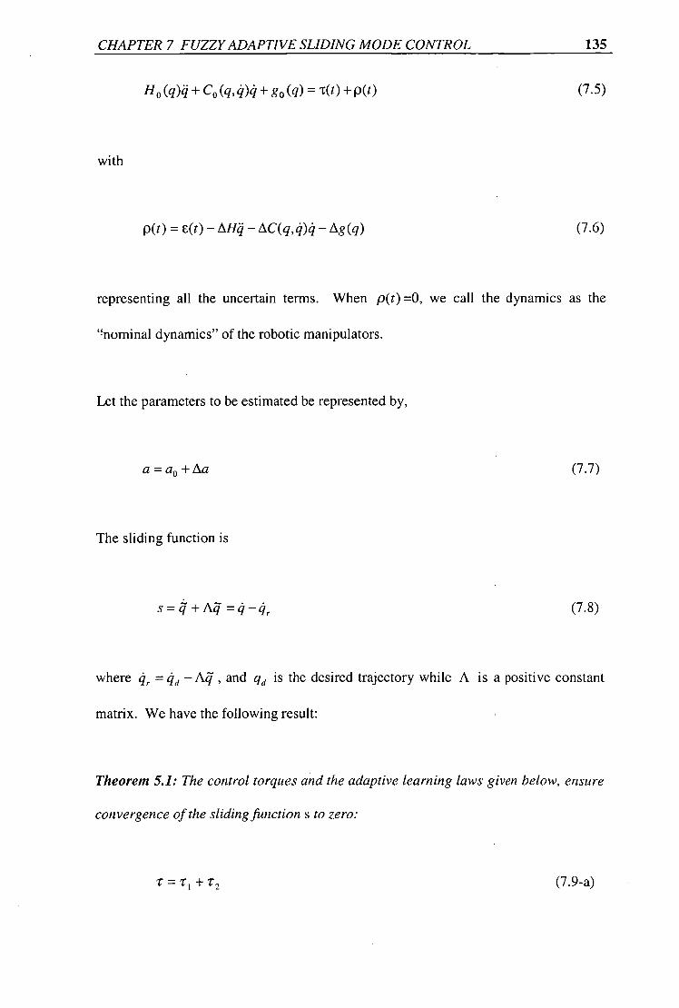
CHAPTER 7 FUZZY ADAPTIVE SLIDING MODE CONTROL 135
H0(q ) .4+ co (q,4)4+ go(q)= t(t)+P(t)
(7.5)
with
p(t)=E(t)— AC(q,q)q— Ag(q) (7.6)
representing all the uncertain terms. When p(t)=0, we call the dynamics as the
”nominal dynamics" of the robotic manipulators.
Let the parameters to be estimated be represented by,
a= a0 + Aa (7.7)
The sliding function is
s= 4 + = (7.8)
where 4,. = 4„ — A, and qd is the desired trajectory while A is a positive constant
matrix. We have the following result:
Theorem 5.1: The control torques and the adaptive learning laws given below, ensure
convergence of the sliding function s to zero:
(7.9-a)

CHAPTER 7 FUZZY ADAPTIVE SLIDING MODE CONTROL 136
r, = ya— Ks, (7.9-b)
T 2 = —Qsgn(s) (7.9-c)
= —FY T s, (7.10)
where Y is the regressor matrix satisfying
Ho4 r + C0q + go = Ya o
K is a positive definite constant matrix, a the estimated parameter, = a — a0 , Q the
upper bound matrix for p(t), and r a constant positive definite matrix.
Proof: To analyse the convergence and stability, we consider the Lyapunov function
v(t)=—(sT H o s+ c-i- Tr - ia) 2
(7.11)
The derivative of V(t) is
•:-T —- IY(t)= S T Hcri.-F 1 —2 sT flos+a r I a (7.12)
Substituting = q - 4,. and Ho = H — All yields
1Y(t)= 5 T (H4 —AH4 —H04,)+-21 s T ilo s+ (7.13)
Since H.4 + C4 + g = + E. therefore

CHAPTER 7 FUZZY ADAPTIVE SLIDING MODE CONTROL 137
1/4 = T E — (Co + AC)4 — (g o + Ag) (7.14)
So, we have
— Co 4 — g o ) + —21 s r fl o s+a T r -t a- (7.15)
1 - Now, using s = 4-4, and —s T (H0 —2C0 )s = 0 (Slotine and Sastry, 1987, 1991) we 2
have
sT (_coo + _21 s T fios = Ths T cos + _21 sT sT co4r _ sT co4r,
Substituting r = T 1 + T 2 we get
IY(t) = s r ('r, — H ø 4 r — — g o ) + s r (T 2 + p) + (7.16)
Since HA, + C0q + go = Yao and (7.9)-(7.10), therefore
1(t) = s r (Ya — Ks —Ya o )+ EL T r -i a + sT (T 2 + p). (7.17)
But sr sgn(s) = Choosing a T _ (_ryT T ) _S T }T, we have

CHAPTER 7 FUZZY ADAPTIVE SLIDING MODE CONTROL 138
T A a r a =—s Yl 1 (a — a0 ) . (7.18)
Therefore
V(t)=—s T Ks— sr p+ ST t ,
= —s T Ks— s T p— s T Qsgn(s) < 0
(7.19)
Tracking convergence is then proved, i.e. s --> . QED.
Remark 7.1: From (7-9) one can see that the control torque contains two parts: 1 1 is
identical to the control law of Slotine and Li (1987; 1991) which is used to estimate
the constant part of the system parameters; the other part r 2 is the switching control
characterised by upper bound matrix Q for system uncertainties and external
disturbances.
Remark 7.2: In order to achieve the good quality of the above adaptive sliding mode
control, we apply the same fuzzy tuning mechanism as described in Section 5.3 to
adjust switching control parameter Q according to Lyapunov function and its time
derivative.
The fuzzy inference system consists of two linguistic input variables V and V and one
linguistic output variable Q. The two fuzzy input variables are defined as follows

CHAPTER 7 FUZZY ADAPTIVE SLIDING MODE CONTROL 139
V={B, M, S} (7.20)
V=113 , Z, (7.21)
where B = big, M = medium, S = small, P = positive, Z = zero, N = negtive. Fuzzy
output variable Q is defined as follows
Q={B, MB, M, MS, S} (7.22)
where MB = medium big, MS = medium small. The input-output relation of the fuzzy
controller with fuzzy variables (7.20), (7.21) and (7.22) is written by
V, —>Q (7.23)
The fuzzy tuning algorithm for Q is described in following fuzzy rules,
1'. If (V is B) and ( V is P) then (Q is B)
2. If (V is B) and ( V is Z) then (Q is MB)
3. If (V is B) and ( V is N) then (Q is M)
4. If (V is M) and ( V is P) then (Q is MB)
5. If (V is M) and ( V is Z) then (Q is M)
6. If (V is M) and ( V is N) then (Q is MS)
7. If (V is S) and ( V is P) then (Q is M)
8. If (V is S) and ( V is Z) then (Q is MS)
9. If (V is S) and ( V is N) then (Q is S)
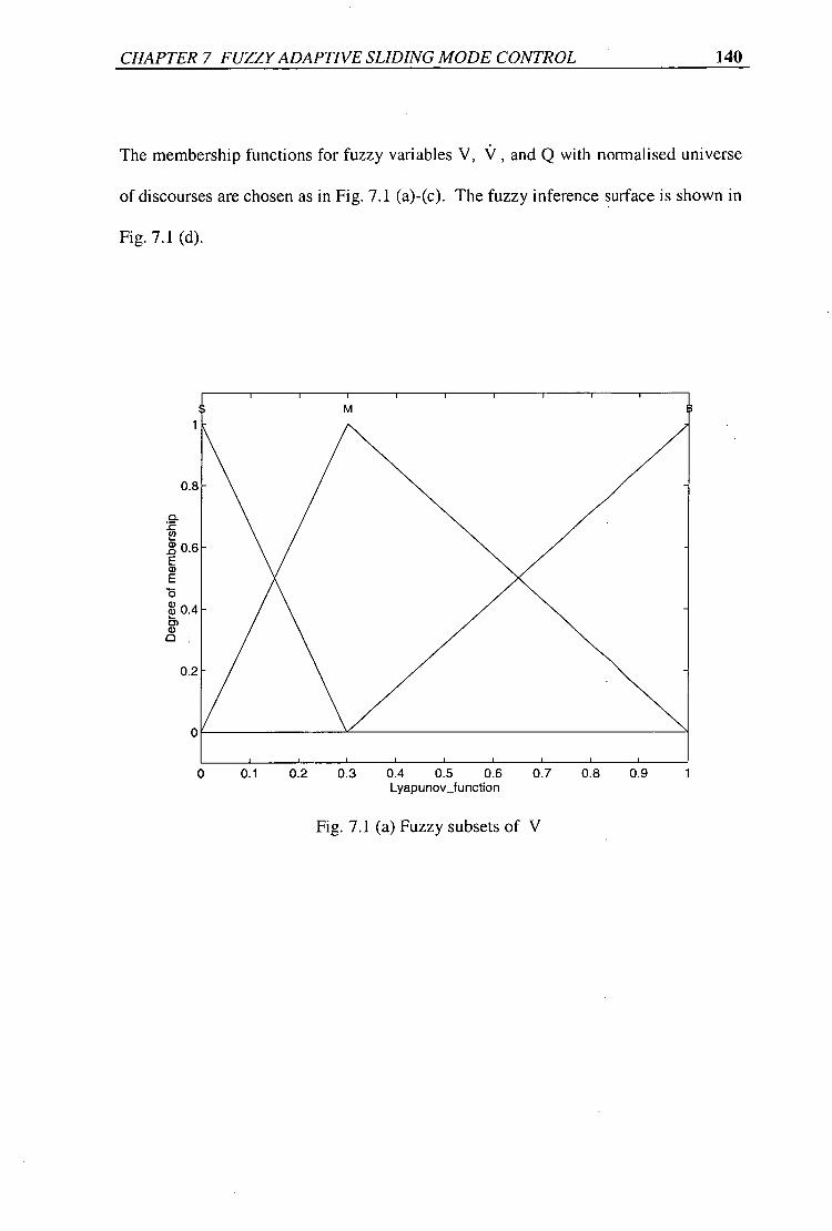
CHAPTER 7 FUZZY ADAPTIVE SLIDING MODE CONTROL 140
The membership functions for fuzzy variables V, V, and Q with normalised universe
of discourses are chosen as in Fig. 7.1 (a)-(c). The fuzzy inference surface is shown in
Fig. 7.1 (d).
0.8
Isn
0.2
0 0.1 0.2 0.3 0.4 0.5 0.6
0.7
0.8
0.9 Lyapunov_function
Fig. 7.1 (a) Fuzzy subsets of V

CHAPTER 7 FUZZY ADAPTIVE SLIDING MODE CONTROL 141
0.6 1 0.8 -0.8 -0.6 -0.4 -0.2 0 0.2 0.4 Change_rate_of_Lyapunovf unction
Fig. 7.1 (b) Fuzzy subsets of V
MB
0.8 0.9 1 0.7 0 0.1 0.2 0.3 0.4 0.5 0.6 Control_parameter_Q
1
0
Fig. 7.1 (c) Fuzzy subsets of Q
0.8
0.2
1
0.8
0.2
0
S M

CHAPTER 7 FUZZY ADAPTIVE SLIDING MODE CONTROL 142
V_dot V
Fig. 7.1 (d) Surface of Q (V, V)
7.3 An illustrative example
A real-time implementation of the control strategy was developed for a five-bar
robotic manipulator, as shown in Fig 7.2.
Fig.7.2 A five bar robotic manipulator

Computer Pentium Pro
PC-30D
PCL-833
DC-Tacho/Encoder
Servo amplifier
DC-Tacho/Encoder
Motor 2 Motor 1 Robot
arm
CHAPTER 7 FUZZY ADAPTIVE SLIDING MODE CONTROL 143
The dynamics of the resultant two degree of freedom system, operating in the
horizontal plane, can be approximately described by
[H 11 [H 2 ,
H 12 1[ 41 [ 0 4 2 4 1 . T i
H22 42 /141 0 42 Lt 2 (7.24)
where H il = a 1 , H 12 = H 21 = —a 3 cos(q 2 — ) H 22 = a 2 , h = a 3 sin(q 2 — q l ) •
The hardware details are shown in Fig. 7.3. Two interface cards are installed in the
computer with a Pentium Pro/200MHz CPU. The PC-30D by Eagle Tech consists of
two 12-bit D/A converters with full scale output range from 0 to +10V, the output
signals are fed to robot motors through a Servo amplifier by Baldor (TSD-050-05-02-
1, operated in torque mode). The PCL-833 by Advantech is a 3-axis quadrature
encoder and counter add-on card, and receives qradrature signals from DC-
Tacho/Encoders (with 500 counts/rev) mounted on the motor shafts for joint angle
measurements. DC motors by Maxon (RE035-071-39, gear ratio 86:1) provide the
joint actuation.
Fig. 7.3 Schematic diagram of the five -bar robot

CHAPTER 7 FUZZY ADAPTIVE SLIDING MODE CONTROL 144
The following second order dynamic model was chosen to generate the desired
trajectory:
X m = A„,x„, +B„,r
where x. = [qd , qd2 qd1 qd2 f , with initial values x„,(0) = [2.0 1.5 0 0] T
0 0 1 0 0 0 0 1
—6.25 0 —5 0 0 —6.25 0 —5
and r(t) is the set point.
The initial state of the robot was chosen as
[q1 q2 41 42f =[- 0 0 of
The initial estimates of the system parameters were chosen as
[a l a2 a3 ]T = [0.02 0.04 0.0015]T
The following parameters were also chosen
A m = B„, =
00 00 10 01

CHAPTER 7 FUZZY ADAPTIVE SLIDING MODE CONTROL 145
K = 21, A =10/,
0.01 0 o 1= o 0.01 o
o o 0.001
In this experiment, the sampling interval is lms.
Fig. 7.4- 7.10 show the experimental results with T 2 = —Q sgn(s) and Q=0.5 without
fuzzy tuning. It is observed that there exists chattering in the control signal.
Fig. 7.11- 7.17 show the experimental results with T 2 = —Q sgn(s) and Q„..0.5 with
fuzzy tuning. It is observed that the control chattering is diminished.
7.4 Concluding remarks
In this chapter, Lyapunov stability theory and fuzzy logic technique are combined
together to design fuzzy adaptive sliding mode control systems. It is shown that an
adaptive sliding mode control is first designed to learn the system parameters with
bounded system uncertainties and external disturbances. A set of fuzzy rules are then
used to adjust the controller's uncertainty bound based on the Lyapunov function and
its time derivative. The robust adaptive sliding mode controllers with fuzzy tuning
algorithm show the advantage of reducing the chattering and the amplitude of the
control signals, compared with the adaptive sliding mode controller without fuzzy
tuning. Experimental example for a five-bar robot arm is given in support of the
proposed control scheme.

CHAPTER 7 FUZZY ADAPTIVE SLIDING MODE CONTROL 146
3.2
—2.8 -o Et_ 2 2.6
"5
set point — model reference - - system response
0 2 1.8
1.6
1.4
0 2 4 6 8 10 12 14 16 18 20 time (s)
Fig. 7.4 Output tracking of joint 1(without fuzzy tuning)
The
outp
ut tr
acki
ng o
f joi
nt tw
o (r
a d)
-0.2
0.6
0.4
0.2
0.8
1.2
1.6
1.4
1
set point — model reference
- system response
0
2
4 6 8 10 12
14 16 18 20 time (s)
Fig. 7.5 Output tracking of joint 2(without fuzzy tuning)

16 18 20 14 2 4 6 8 10 12 time (s)
0.02
0.015
Ca 0.01
.5
•
0.005
5 C. 5 a) -0.01 .c
- 0.015
CHAPTER 7 FUZZY ADAPTIVE SLIDING MODE CONTROL 147
0.02
0.015
Ca
a) 0.01
•6 0.005 "6
- 0.015
-0.02 0
, 1
2 4 6 8 10 12 time (s)
14 16 18 20
Fig. 7.6 Tracking error of joint 1 (without fuzzy tuning)
Fig. 7.7 Tracking error of joint 2 (without fuzzy tuning)

CHAPTER 7 FUZZY ADAPTIVE SLIDING MODE CONTROL 148
1.5 -
1111111110111L1 11 11 11111 1 1
-1.5 -
-20
2 4 6 8 10 12 14 16 18
20 time (s)
Fig. 7.8 Control input of joint 1 (without fuzzy tuning)
1.5
2 0.5
.0
0. II 11111111.11M11111111111111111 111111111111
•-
-0.5
ci
_
-1.5
■ ■ ,
2 4 6 8 10 12 14 16 . 18 time (s)
Fig. 7.9 Control input of joint 2 (without fuzzy tuning)
20

3.2
3
—2.8 -o
2.6
1.6
1.4
set point — model reference
- system response
CHAPTER 7 FUZZY ADAPTIVE SLIDING MODE CONTROL 149
Parameter estimations 0.06
0.05
al — a2 - - a3
0.02
0.01 r-
Oo 2 4 6 8 10 12
time (s)
Fig. 7.10 Parameter estimations (without fuzzy tuning)
2 4 6 8 10 12 14 16 18 20 time (s)
0.04
0.03
14 16 18 20
Fig. 7.11 Output tracking of joint 1 (with fuzzy tuning)

CHAPTER 7 FUZZY ADAPTIVE SLIDING MODE CONTROL 150
The
outp
ut tr
acki
ng o
f joi
nt tw
o (ra
d)
1.6
1.4
1.2
1
0.8
0.6
0.4
0.2
-0.2
0 2 4 6 8 10 12 14 16 18 20 time (s)
Fig. 7.12 Output tracking of joint 2 (with fuzzy tuning)
0.02
0.015 -
13 Ca
0.01 - a)
:5 0.005 - "5
‘6: if) 0)
Ez, -0.005 - 5 5 ° -0.01 - a) _c
-0.015 -
-0.02 0
2 4 6 8 10 12 14 16 18 time (s)
20
Fig. 7.13 Tracking error of joint 1 (with fuzzy tuning)
set point
— model reference
- system response

CHAPTER 7 FUZZY ADAPTIVE SLIDING MODE CONTROL 151
0.02
0.015
=-6 Ca
0.01
.5
▪
0.005
;(2
C.)
-0.005 5 a.
a) -0.01 .c
- 0.015 -
-0.02 0 20 2 4 6 8 10 12 14 16 18
time (s)
Fig. 7.14 Tracking error of joint 2 (with fuzzy tuning)
1.5
- 1.5
■ , , ,
2 4 6 8 10 12 14 16 18 time (s)
20
Fig. 7. 15 Control input of joint 1 (with fuzzy tuning)

al — a2 - - a3
• .............................. . ...............................................................
CHAPTER 7 FUZZY ADAPTIVE SLIDING MODE CONTROL 152
1.5
0.5
.0 "5
• -0.5
-1.5
-20 20 2 4 6 8 10 12 14 16 18
time (s)
Fig. 7.16 Control input of joint 2 (with fuzzy tuning)
Parameter estimations
0.01
0.03
0.02
0.06
0.05
0.04
0 0 2 4 6 8 10 12
time (s) 14 16 18 20
Fig. 7.17 Parameter estimations (with fuzzy tuning)

CHAPTER 8 ROBUST ADAPTIVE SLIDING MODE CONTROL OF ROBOTS 153
Chapter 8
Robust Adaptive Sliding Mode Control of Robots
8.1 Introduction
Adaptive control of mechanical manipulators has been studied extensively by many
researchers using various methodologies (Craig et al., 1986; Slotine and Sastry, 1984;
Balestrino et al., 1979; Young, 1978), such as hyperstability theory, Lyapunov
stability method, self-tuning regulator control and sliding mode control (SMC).
Among the various methodologies, the SMC demonstrates its good robustness and low
computational cost. SMC is a discontinuous feedback control that switches the system
control structure during the evolution of the system state so that the system states
remain in a prescribed subspace. A SMC controller for robot manipulators suggests
that each manipulator link matches a first order sliding motion such that when the
system state reaches the sliding mode, it chatters along the sliding mode and exhibits
insensitivity to the system parameter variations and external disturbances (Slotine &
Li, 1987).

CHAPTER 8 ROBUST ADAPTIVE SLIDING MODE CONTROL OF ROBOTS 154
One of the well known results in SMC design for trajectory tracking of robotic
manipulators was obtained by Slotine and Li (1987, 1991). Their adaptive SMC is
based on the linear parametrisation approach for the robotic systems which do not
involve any uncertainties and disturbances. The validity of the control algorithm is
based on the assumption that the system parameters must be constant and the desired
trajectory should be sufficiently "rich" to guarantee parameter convergence. To
overcome the robustness problem of Slotine and Li's controller, Su and Leung (1993)
have proposed a modification that employs the bound estimation algorithms in the
controller to give rise to a robust adaptive SMC controller without a priori knowledge
of upper bounds of the system parameters. This controller is able to handle large and
time varying variations in the parameters. However, the problem is that their control
torques designed incur very large chattering which is not desirable in practice,
especially in mechanical systems.
In this chapter, a new adaptive SMC law is proposed for trajectory tracking of rigid
robotic manipulators with uncertainties to achieve robustness as well as desired
qualities such as speedy tracking, minimal chattering and small control torques. We
first show that, under a mild assumption, and if the control input does not contain the
acceleration signal, then the system uncertainty is bounded by a positive function of
the position and velocity measurements. This result forms the foundation of the
derivation of the proposed adaptive SMC law which does not require measurement of
acceleration signals. We then propose an adaptive SMC strategy that integrates the
Slotine and Li's controller for estimation of the constant part of the system parameters
with a switching controller that takes care of the uncertain part of the system
parameters with its switching amplitude adaptively learned by a Gaussian RBF neural

CHAPTER 8 ROBUST ADAPTIVE SLIDING MODE CONTROL OF ROBOTS 155
network. The advantage of the proposed adaptive SMC strategy is that the switching
control part only controls the "real" uncertain part of the system parameters, and the
minimum control effort is achieved by adaptive learning of the uncertainty bound.
When the magnitude of the uncertainties is small, the chattering caused by the
switching is small.
This chapter is organised as follows: In Section 8.2, the robust adaptive SMC design is
presented. Section 8.3 describes the experimental results for confirmation of the
theoretical results. Section 8.4 gives conclusions.
8.2 The Robust Adaptive SMC Design
Consider the dynamics of the n-joint robotic manipulators represented by the
following second order nonlinear vector differential equation
H (q)ij + C(q,4)4 + g(q) = r(t)+ e(t) (8.1)
where q(t) is the nxl vector of joint angular positions, H(q) is the nxn symmetric
positive definite inertia matrix, C(q,4)4 is the nxl vector containing Coriolis,
centrifugal forces, g(q) represents the derivation of the manipulators potential energy,
r(t) is the nxl vector of applied joint torques which are actually control inputs, and
e(t) is the nxl bounded input disturbances vector.
We assume that the robotic manipulators have uncertainties, i.e.
H (q) = H 0 (q) + AH (q)
(8.2)
C(q,4)= Co (q,4)+ AC(q, 4)
(8.3)

CHAPTER 8 ROBUST ADAPTIVE SLIDING MODE CONTROL OF ROBOTS 156
g(q) = g o (q)+ Ag(q) (8.4)
where H 0 (q),C0 (q,4), g o (q) are the nominal parts and AH (q), AC(q,q), Ag(q) are
the uncertain parts. The uncertain components represent bounded small possible time
varying, unmodelled dynamics or load changes. Substituting the expressions (8.2)-
(8.4) into the dynamics (8.1) gives rise to
Ho (0.4 ± Co (q, 4)4 + go (q) = t(t) + P(t) (8.5)
with
p(t)= e(t)— AI-14— AC(q,q)q — Ag(q) (8.6)
representing all the uncertain terms. When p(t)=0, we call the dynamics as the
"nominal dynamics" of the robotic manipulators.
Some mild assumptions are made prior to further discussion. These assumptions are
usually satisfied in practice.
Assumption 8.1: The matrix H(q) is bounded and invertible, i.e. for some unknown
constant y h ,
(8.7)
and 11 - ' (q) exists for all q.
Assumption 8.2: The vectors C(q,q) and g(q) satisfy
IIC(q Y c20q11 + Y c3I1411 2
lig(q)11<yf +yllq11 where yh of , yC2 , yC3, y f 9 - gg y are positive constants but do not have to be known.
(8.8)
(8.9)

CHAPTER 8 ROBUST ADAPTIVE SLIDING MODE CONTROL OF ROBOTS 157
According to the characteristics of industrial robots, These assumptions are not
stringent and have been used by many researchers (Abdallah et al., 1991). With these
mild assumptions, the following theorem is derived which will be very useful for later
derivation of the robust adaptive SMC controller for robotic manipulators.
Theorem 8.1: With Assumption 8.1-2, if the control input vector t(t)does not contain
the acceleration signal 4, then the system uncertainty term p(t) is bounded by a
positive function of the position and velocity measurements:
1113(0 11 ‹ Ed (q ,4)
(8.10)
where Fd (q,(4) is a positive function to be expressed in the following.
Proof: Expression (8.5) can be written in the following form
4= H0 (q) -1 (T(t)+ p(t))- Ho (q) -I ho (q,q) (8.11)
with hc, = Co (q,q)q + g o (q) . Using expression (8.11) in expression (8.6), we have
p(t)= -AH(q)q - Ah(q,q)+ E(t) = -AH(q)11 0 (q) -1-4t)
-AH(q)H0 (q) -1 p(t)- AH(q)110 (q) -1 110 (q,4)- Ah(q,q)+ E(t) (8.12)
which gives
p(t)= -(1 + AH(q)H0 (q) -1 ) -1 AH(q)H0 (q) - ` 'r(t) +(l + AH(q)110 (q) -1 ) -1 (-Ah(q,4)+ E(t))
-(I + AH(q)H0 (q) -1 ) -1 AH(q)Ho (q) -1 ) -1 AH(q)H0 (q) -1 110 (q,q) (8.13)
Then
10(01 11(I + AI-1(q)H0(q)-'11A11(q)110(q)-'11111011 +V(I + AH(q)H0 (q) - ' )111Ah(q ,q)II II ± A 11(q )110(q )-' ) -1 1010 )11
+ 0 (1 AH(q)110(q )-1)-1 0A11(q )110(q )-1 1111 110( q ')11
(8.14)

CHAPTER 8 ROBUST ADAPTIVE SLIDING MODE CONTROL OF ROBOTS 158
Considering the assumptions 8.1-2 and the fact that the input disturbance vector is
upper bounded, we have the following inequalities:
11(/ + AH(q)H0 (q) -1 ) -1 11< a 1 (8.15-a)
11 AH(q )110(q )-1 11 < a2 (8.15-b)
Ils(t)11‹ Et (8.15-c)
Ilho(q , 4)11 < a3 +a411.711+414112 (8.15-d)
IlAh(q , 4)11 < a 7 + 414 a904112 (8.15-e)
where a 1 ,...,a 9 and E I are unknown positive constants. Using inequalities (8.15-a)-
(8.15-e) in expression (8.14), we have
11 13(t) Il <a l alr(t) 11 (a1a7 atE1 a1a2a3
+(aia8 a1a2a4)11q11
+(a1a9 a1a2a5 )4 11 2
Now because the control input does not contain acceleration signal, i.e.,
t(t) = F(q,4)
and there exists a positive function Fp (q,4) such that
11'0011=11F (q , 4)1I < F p (q , 4) Using expression (8.18) in expression (8.16), we have
a 1 a 2 F p , 4)
± (a l a 7 ± a iE ala2a3 + (alas aia2a4 )114
+ (a1a9 ot1a2a5
Fd(q 7 0
(8.16)
(8.17)
(8.18)
(8.19)
QED.
CHAPTER 8 ROBUST ADAPTIVE SLIDING MODE CONTROL OF ROBOTS 159
Remark 8.1: It has been seen from above discussion that the upper bound of the
system uncertainty p(t) is input-related because of the high nonlinearities in robot
systems.
Remark 8.2: As a special case of theorem 8.1, if the control system uses the following
polynomial-type of controller,
11'0011 < x 0 + x111q 1I+ x211411 2 = F, (q, 4)
(8.20)
where A 0 , X I and A 2 are positive numbers, then by expression (8.19), we have
111)(011 < b1 + NM+ b311411 2
(8.21)
where
bl = a 1 a 2X 0 +a,a, +a,c, +a,a 2a 3 ,
b2 = a 1 a 2X 1 +a 1 a 8 +a,a 2 a 4 ,
b3 =a,a 2X 2 +a,a 9 +a,a 2 a 5 .
Bounded property in expression (8.21) has been used by some researchers (Abdallah
et al., 1991, Man & Palaniswami, 1994).
In order to track a desired trajectory using robotic manipulators whose parameters are
composed of large, fixed parts and small, bounded uncertain parts, we propose a
controller structure that consists of two components: one is switching controller with
amplitude adaptively learned by using Gaussian RBF neural networks which controls
only the uncertain parts; the other is similar to Slotine and Li's controller that takes
care of the certain parts.
Suppose p c, (q,4) is the optimal bounding function for p(t) , i.e.,

CHAPTER 8 ROBUST ADAPTIVE SLIDING MODE CONTROL OF ROBOTS 160
IIP(t)11 Po (.7, 4)
(8.22)
In this paper, we choose the Gaussian RBF neural network to adaptively learn the
bounding function p o (q, 4) . It has been shown (Poggio & Girosi, 1990) that a linear
superposition of Gaussian RBFs results in an optimal mean square approximation to
an unknown function which is infinitely differentiable and whose values are specified
at a finite set of points. Further, it has been proven (Poggio & Girosi, 1990) that any
continuous functions, not necessarily infinitely smooth, can be uniformly
approximated by a linear combination of Gaussian RBFs.
The Gaussian RBF neural network is a particular network architecture (Poggio &
Girosi, 1990) that consists of three layers: the input layer, the hidden layer that
contains the Gaussian RBF and the output layer. At the input layer, the input space
x E R" is divided into grids with a Gaussian function at each node defining a receptive
field in R" with c i as its centre and cs 2 as its variance. The value of variance essentially
defines the extent of localisation of the effect of the input. The approximation of the
bounding function can be written as,
pow = 0 T 4(x)
.ye,(0,(x) (8.23)
where x = [q T • T q , 0 is the weight vector, and
11 X C i 11 2 11) i (X) = exp( 2 )
a (8.24)
Assume that there exists a constant weight vector 0* so that 0* T O(x) achieves the
minimum control effort of the sliding mode control and
0* T 0(x) — p o (x) A (8.25)

CHAPTER 8 ROBUST ADAPTIVE SLIDING MODE CONTROL OF ROBOTS 161
where A is a small positive number.
Let the parameters to be estimated be represented
a = a + Aa (8.26)
The sliding function is s = Fir + = — 4 r (8.27)
where 4, = 4 d — A, and qd is the desired trajectory while A is a positive constant
matrix. We have the following result:
Theorem 8.2: The control torques and the adaptive learning laws given below, ensure
convergence of the sliding function s to zero:
1= + (8.28-a)
T i = Y - Ks, (8.28-b)
T 2 = —6 7- (130(X)sgn(s)
(8.28-c)
a = — ryTs, (8.29)
6 = 0.0(.11s11
(8.30)
where Y is the regressor matrix satisfying
Ho e'fir + C04, + go = Yao
K is a positive definite constant matrix, a the estimated parameter, a = a - ao , 0 the
weight vector for bounding function, Q a positive definite diagonal matrix and r a
constant positive definite matrix.
Proof: To analyse the convergence and stability, we consider the Lyapunov function

CHAPTER 8 ROBUST ADAPTIVE SLIDING MODE CONTROL OF ROBOTS 162
-1 V (t) = r 11 0 S + arr - a + 0 E2 0- 1 2
The derivative of V(t) is
1(t) = s T H 0 ,i• + —21 s r H o s + tirr -ta - 6Tg2 -1 6
Substituting = 4 - 4„ and Ho = H — AH yields
V(t) = S T (114 6.114 — 11 0 4,)+ —21 S T 1 .1 0 S + a rr -t a - 6 7- 52 -1 6
Since 114 + C4 + g = . therefore
(8.31)
(8.32)
(8.33)
H4 = T - ( C0 + AC)4 - (g0 + (8.34)
So, we have
1(t)= S T — AH4 — AC4 — Ag — Ho ii r — Co4 —g o ) + —21 S T fl o S± a T r --' - -OTS-116
(8.35)
1 Now, using s = 4 - 4 and —s T (H0 —2C0 )s = 0 (Slotine & Li, 1987; 1991) we have
r 2
s T c r c r S T ( —004)+ —21 S T 1110 S = — S T Co S + —21 /los _ sT o4 = _ sr o4 ,
Substituting r = r 1 + T 2 we get
(8.36)
Since HA + C04,. + g o = Yao and (8.28)-(8.30), therefore
1(t) = sr (Ya— Ks —Ya0 )+ arr -ia - -OTE-21
+sr(1- 2 - - Ac4 - Ag).
But ST sgn(s) = IsO, Choosing aT =, )T sT Yr, we have
(8.37)

CHAPTER 8 ROBUST ADAPTIVE SLIDING MODE CONTROL OF ROBOTS 163
• — a i a = —sT yrr - '(â--- a0 ) .
Therefore
1Y = -S T Ks — s T (6.114 Ag)— s T o T (I)(q,q)sgn(s) — ii T S2 -1 6
= —s T Ks — sTp(t)— 61'4014 - (CI* - T 4)(14 5_ — s T Ks — [0 *T (1(x) P 0(X)1114 < 0
(8.38)
(8.39)
Tracking convergence is then proved, i.e. s --> 0. QED.
Remark 8.3: From (8.28) one can see that the control torque contains two parts: one
is identical to the control law of Slotine and Li (1987;1991) which is used to estimate
the constant part of the system parameters; the other part is an adaptively learned
switching control by using the Gaussian RBF network. The validity of the
combination of these two control structures lies in theorem 1 which ensures that the
uncertainty can be represented in terms of q and 4. The advantage of the proposed
controller is that the minimum control effort can be achieved by adaptively learning
of the bounding function, thus, when the magnitude of uncertainties is small, the
magnitude of chattering is small.
8.3 Experimental Results
To demonstrate the validity of the proposed robust algorithm (8.28)-(8.30), a real-time
implementation of the control strategy was developed for a five bar robotic
manipulator similar in design to that used by a number of researchers (Mills and
Lockhorst,1993; Gourdeau and Schwartz, 1991). As shown in Figure 8.1, the links of

/1421411 , [ Ill 0 4 2 T 2
[HII HI21[411+
[H21 H22 42 h41
CHAPTER 8 ROBUST ADAPTIVE SLIDING MODE CONTROL OF ROBOTS 164
the robot form a parallelogram enabling the position of the end effector to be uniquely
specified by the rotations of links one and two.
Fig.8.1 A five bar robotic manipulator
The dynamics of the resultant tWo degree of freedom system, operating in the
horizontal plane, can be approximately described by (Mills and Lockhorst, 1993)
where H i =a, H12 = H2I = —a 3 cos(q 2 — ) 7 H22 = a 2 , h = a 3 sin(q 2 — q, ) .
The following second order dynamic model was chosen to generate the desired
trajectory:
= A mx. +B m r
where x„, = [qdi qd2 (*h i qd2 f , with initial values x„, (0) = [2.0 1.5 0 Of

Computer Pentium Pro
PC-30D
PCL-833
DC-Tacho/Encoder
Servo amplifier
DC-Tacho/Encoder
Motor 1 Motor 2
Robot arm
CHAPTER 8 ROBUST ADAPTIVE SLIDING MODE CONTROL OF ROBOTS 165
=
0 0
—6.25 0
0 0 0
—6.25
1 0
—5 0
0 1 0
—5
B =
00 00 10 01
and r(t) is the set point.
The hardware details of the control system are shown in Figure 8.2. Two interface
cards are installed in the computer with a Pentium Pro/200MHz CPU. The PC-30D by
Eagle Tech consists of two 12-bit D/A converters with full scale output range from 0
to +10V, the output signals are fed to robot motors through a Servo amplifier by
Baldor (TSD-050-05-02-1, operated in torque mode). The PCL-833 by Advantech is a
3-axis quadrature encoder and counter add-on card, and receives qradrature signals
from DC-Tacho/Encoders (with 500 counts/rev) mounted on the motor shafts for joint
angle measurements. DC motors by Maxon (RE035-071-39, gear ratio 86:1) provide
the joint actuation.
Fig.8.2 Schematic diagram of robot control system

CHAPTER 8 ROBUST ADAPTIVE SLIDING MODE CONTROL OF ROBOTS 166
The initial state of the robot was chosen as
[ql q2 41 421 = [i 00 of
The initial estimates of the system parameters were chosen as
[a l a 2 a 3 f = [0.015 0.04 0.0015r
The centres of the Gaussian RBFs were chosen as follows: 1.4 and 3.4 for q,, 0 and
2.0 for q 2 , -1 and 1 for 4 1 and 4 2 . Therefore, totally 2x2x2x2 =16 Gaussian RBFs
were used in the experiment.
The following parameters were also chosen
K = 21, A =10/, S2 = 21, a 2 = 2.0
0.01 0 0 F= 0 0.01 0
0 0 0.001 _
In this experiment, the sampling interval is lms. Figure 8.3(a)-(c) show the graphs of
the output tracking, tracking errors and control torques. Figure 8.4 shows the
parameter estimations. Figure 8.5 illustrates the bounding function estimations.

CHAPTER 8 ROBUST ADAPTIVE SLIDING MODE CONTROL OF ROBOTS 167
8.4 Concluding remarks
A new adaptive sliding mode controller has been developed in this chapter for
trajectory tracking in robotic manipulators. This controller is able to estimate the
constant part of the system parameters as well as adaptively learn the uncertain part of
the system parameters by the Gaussian neural network. We have shown that under a
mild assumption, the proposed control law does not require measurement of
acceleration signals. This new control law exhibits the good aspects of Slotine and
Li's and keeps the chattering to a minimum level. An experiment with a five bar
robotic system was done and the results have confirmed the effectiveness of the
approach.

set point • model reference
system response
2 4 6 8 10 time (s)
12 14 16 18 20
Fig. 8.3(a) The output tracking of joint one and two.
CHAPTER 8 ROBUST ADAPTIVE SLIDING MODE CONTROL OF ROBOTS 168
3.2
2.8
CRT 2.6
'5 2.4
Ye 2.2 Co
o. 2
set point model reference system response
1.6
1.4
2 4 6 8 10 time (s)
12 14 16 18 20
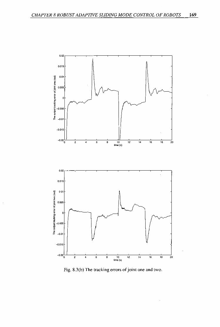
CHAPTER 8 ROBUST ADAPTIVE SLIDING MODE CONTROL OF ROBOTS 169
0.02
0.015 -
0.01
0.005
F Ca
-0.005 0. 0
-0.01
- 0.015
- 0.02
0
2 4 6 8 10
12 14 16 18 20 time (s)
0.02
0.015
▪ 0 01
0.005
I-- -0.01
- 0.015 -
■ , . , .
2 4 6 8 10 12 14 16 18 time (s)
- 0.02 0
Fig. 8.3(b) The tracking errors of joint one and two.
20

CHAPTER 8 ROBUST ADAPTIVE SLIDING MODE CONTROL OF ROBOTS 170
1.5 -
c 0 5
rEVL- •E
-g, -0.5 - C.,
-1.5-
2 4 6 8 10 12 14 16 18 20 time (s)
1.5-
3 0.5
5 frimui tam 1r--4-"---1
72
a)
-1.5 -
2 4 6 8 10 12 14 16 18 t 1 1 I i 1
20 time (s)
Fig. 8.3(c) The control inputs of joint one and two.

0.06
0.05
0.04
-
_
_ al a2 a3
0.03
0.02 -
0.01 - ,
2 4 6 8 10 12 time (s)
oo 14 16 18 20
CHAPTER 8 ROBUST ADAPTIVE SLIDING MODE CONTROL OF ROBOTS 171
Parameters estimation
Fig. 8.4 The system parameters estimations
Bounding function estimation
%./^%,.......
2 4 6 8 10 12 14 16 18 20 time (s)
0.7
0.6
0.5
0.4
0.3
0.2
0.1
Fig. 8.5 Bounding function estimation

CHAPTER 9 CONCLUSIONS 172
Chapter 9
Conclusions
9.1 Summary
Variable structure control technique is a powerful approach for the control of
nonlinear systems. It is advocated to solve complex control problems that are not in
the scope of simple linear feedback controllers and adaptive controllers. However, the
over estimation of system uncertainties and the inherent control chattering will still be
the main issue of the variable structure controller design. Therefore, this thesis has
been mainly concerned with the study and improvements of robust control schemes by
employing artificial intelligent technologies.
Chapter two of this thesis has provided a brief survey of variable structure control
theory. Robust variable structure controller design for robotic manipulators has been
presented by using reaching law method. The limitations of these results have also
been highlighted.
Chapter three has provided a background for fuzzy logic and fuzzy logic control
techniques being applied in the thesis. Fuzzy sets, fuzzy set operations, and fuzzy

CHAPTER 9 CONCLUSIONS 173
linguistic representation such as linguistic variables and linguistic modifiers (hedged)
have been briefly outlined. The advantages and disadvantages of fuzzy logic controller
have been discussed.
In chapter four, a robust tracking control scheme is proposed for a class of nonlinear
systems. A nominal fuzzy system model for a nonlinear system is established by fuzzy
synthesis of a set of linearised local subsystems, where the conventional linear
feedback control technique is used to design a feedback controller for the fuzzy
nominal system. A variable structure compensator is then designed to eliminate the
effects of the approximation error and system uncertainties. Strong robustness with
respect to large system uncertainties and asymptotic convergence of the output
tracking error are obtained.
In chapter five, Lyapunov stability theory and fuzzy logic technique are combined
together to design sliding mode control systems. It is shown that a sliding mode is
first designed to describe the desired system dynamics for the controlled system. A set
of fuzzy rules are then used to adjust the controller's parameters based on the
Lyapunov function and its time derivative. The desired system dynamics are then
obtained in the sliding mode. The sliding mode controllers with fuzzy tuning
algorithm show the advantage of reducing the chattering of the control signals,
compared with the conventional sliding mode controllers. The fuzzy tuning algorithm
has also been applied to the adaptive sliding mode control.
In chapter six, a robust continuous sliding mode control scheme for linear systems
with uncertainties has been developed. The controller consists of three components:

CHAPTER 9 CONCLUSIONS 174
equivalent control, continuous reaching mode control and robust control. It retains the
positive properties of sliding mode control but without the disadvantage of control
chattering. The proposed control scheme has been applied to the tracking control of a
one-link robotic manipulator by fuzzy modelling of the nonlinear system.
In chapter seven, Lyapunov stability theory and fuzzy logic technique are combined
together to design fuzzy adaptive sliding mode control systems. It is shown that an
adaptive sliding mode control is first designed to learn the system parameters with
bounded system uncertainties and external disturbances. A set of fuzzy rules are then
used to adjust the controller's uncertainty bound based on the Lyapunov function and
its time derivative. The robust adaptive sliding mode controllers with fuzzy tuning
algorithm show the advantage of reducing the chattering and the amplitude of the
control signals, compared with the adaptive sliding mode controller without fuzzy
tuning. Experimental example for a five-bar robot arm is given in support of the
proposed control scheme.
In chapter eight, a new adaptive sliding mode controller has been developed in this
chapter for trajectory tracking in robotic manipulators. This controller is able to
estimate the constant part of the system parameters as well as adaptively learn the
uncertain part of the system parameters by the Gaussian neural network. It is shown
that under a mild assumption, the proposed control law does not require measurement
of acceleration signals. This new control law exhibits the good aspects of Slotine and
Li's (1987) and keeps the chattering to a minimum level. An experiment of a five bar
robotic system was done and the results have confirmed the effectiveness of the
approach.

CHAPTER 9 CONCLUSIONS 175
In summary, the thesis has provided several new and improved robust variable
structure control schemes by employing fuzzy logic and neural networks technologies
aimed at achieving robustness and convergence with optimised control input in the
presence of system uncertainties and external disturbances. These results have been
applied to robotic manipulators and have been proved both in simulation and
experiment.
9.2 Suggestions for further work
Some areas for further research related to the thesis are:
(1) The sliding mode control technique may be used for the design of adaptive filters.
For example, a Lyapunov function of the tracking error between desired signal and
output of the filter can be defined first. Then the adaptation law of the filter
parameters can be obtained based on the sliding mode control theory, so that the
tracking error can asymptotically converge to zero. The potential advantages of the
sliding mode technique based adaptive filters over the existing LMS and RLS
algorithms would be the simplicity and robustness.
(2) The sliding mode control method may be used for the real time training of neural
networks parameters to improve the convergence and robustness properties. A
Lyapunov function of the error between the desired and actual outputs of the
neural networks can be defined first. Then the error is backward-propagated based
on Lyapunov stability theory so that the weights of the inner layers of the neural
networks can be adjusted adaptively. The distinct advantage over the standard BP
or modified BP would be that the system will not get stuck in a local minimum.

CHAPTER 9 CONCLUSIONS 176
(3) The approach of the terminal sliding mode (Man et al., 1994, Yu et al., 1996) may
be used for BP training of weights of neural networks. As in terminal sliding mode
design, we can replace the inertial term by following form (LiMin Fu, 1991,
PP- 83 ),
Wii (t + 1) = W ji (t)+ 775 J O, + a[W ii (t) —147 ji (t —1)] ql p
The convergence and robustness performance could be expected to be improved.
(4) Last, but not least, fuzzy set theory may be used in the design of fuzzified linear
sliding mode control and terminal sliding mode control. When the system is far
from the desired sliding mode, linear sliding mode control scheme can be used to
achieve fast convergence, while the system is getting closer to the desired sliding
mode, the terminal sliding mode control scheme can be used to guarantee finite
time convergence property. Therefore, optimal system performance can be
achieved by fuzzified control strategy.

REFERENCES 177
References
Abbass, A. F., and Ozguner, U. (1985). Decentralised model reference adaptive
system using a variable structure control. Proc. 24th Conf. Decision & Control,
pp. 1473-1478.
Abdallah, C., and Jordan, R. (1990). A positive-real design for robotic manipulators.
Proc. IEEE Amer. Contr. Conf. pp. 991-992.
Abdallah, C., Dawson, D., Daorato, P., and Jamshidi, M. (1991). Survey of robust
control for rigid robotics. WEE Control Systems, vol. AC - 11, pp. 24-30.
Ambrosino, G., Celentano, G., and Garofalo, F. (1984). Variable structure model
reference adaptive control systems. Int. J. Control, vol. 39, pp. 1339 - 1349.
Amestegui, M. R., Ortega, R., and Ibarra, J. M. (1987). Adaptive linearizing-
decoupling robotic control: a comparative study of different parametrizations.
Proc. 5th Yale Workshop on Applications of adaptive systems theory, New
haven, Connecticut.
Anderson, B. D. 0.et al. (1989). Stability of Adaptive Systems: passivity and
Averaging Techniques. Englewood Cliffs, NJ: Prence - Hall.
Astrom K. J., Hang C. C., Persson P., and Ho W. K. (1992). Toward intelligent HD
control. Automatica, Vol. 28, No. 1, pp. 41-53.
Bahnasawi, A. A., Eid, S. Z., and Mahmoud, M. S. (1991) Adaptive model-
following control based on variable structure systems. Int. J. Systems Sci., vol.
22, pp. 333 - 349.

REFERENCES 178
Baily, E., and Arapostathis, A. (1987). Simple sliding mode control scheme applied to
robot manipulators. Int. J. Contr., vol. 45, pp. 1197-1209.
Balestrino, A., DeMaria, G. and Seiavicco, L. (1979). An adaptive model following
control for robot manipulators. J. Dynamic Systems, Measurement and
Control, Vol.15, pp143-152.
Barmish, B. R., Petersen, I. R., and Fever, A. (1983). Linear ultimate boundedness
control of uncertain dynamical systems. Automatica, vol. 19, pp. 523-532.
Bartolini, G., and Zolezzi, T. (1985). Variable structure nonlinear in the control law.
IEEE Trans. Automat. Contr. vol. AC-30, pp. 681-684.
Becker, N., and Grimm, W. M. (1988). On L2 and L. stability •approaches for the
robotic manipulators. IEEE Automat. Contr., vol. AC-33, pp. 118-122.
Bengiamin, N. N., Kauffmann, B. Variable structure position control. Contr. Syst.
Mag., pp. 3 - 8.
Bondi, P., Casalino, G., and Gambardella, L. (1988) On the iterative learning
control theory for robotic manipulators. IEEE J. Robotics and Automation.
vol. 4, pp. 14 - 22.
Bremer, H. (1985). Parameter-insensitive swivel control of an industrial robot.
Automatisierungstechnik, vol. 33, pp. 74 - 81, (written in German).
Canudas De Wit, C., and Slotine, J-J. E. (1991). Sliding observers for robotic
manipulators. Automatica, vol. 27, pp. 859 - 864.
Canudas de Wit, C., and Fixot, N. (1991). Robot control via robust estimated state
feedback. IEEE Trans. Automat. Contr., vol. AC-36, pp. 1497 - 1501.
Cao S. G., Ree N. W. and Feng G. (1994). Stability analysis of fuzzy control systems.
Proceedings of the IEEE 2nd Australian and New Zealand Conference on
Intelligent Information Systems (ANZIIS-94), Brisbane, Australia, pp. 219-
223.
REFERENCES 179
Cao, S. G., Rees, N. W., Feng, G. (1996). Stability analysis and design for a class of
continuous-time fuzzy control systems. Int. J. Control, vol. 64, pp. 1069-1087,
1996.
Chang, L. W. (1991). A MIMO sliding control with a first-order plus integral sliding
condition. Automatica, vol. 27, pp. 853 - 858.
Chang, S. S. L., and Zadeh, L. A. (1972). Fuzzy mapping and control. IEEE Trans.
Syst., Man, Cybern., Vol. SCM-2, No. 1, pp.30-34.
Corless, M. J. (1989). Tracking control for uncertain systems: application to a manutec
r3 robot'. ASME J. Dynamic System, Measurement, and Control, vol. 111,
pp. 609 - 617.
Corless, M. J., and Leitmann, G. (1981). Continuous state feedback guaranteeing
uniform ultimate boundedness for uncertain dynamic systems. IEEE Trans.
Automat. Contr., vol. AC-26, pp. 437 - 443.
Cox E. (1994). The fuzzy systems handbook. Cambridge, MA: AP Professional.
Crag, J. J., Hsu, P., and Sastry, S. S. (1986). Adaptive control of mechanical
manipulators. IEEE Int. Conf. on Robotics and Automation, pp. 190-195.
Crag, J. J., Hsu, P., and Sastry, S. S. (1987). Adaptive control of mechanical
manipulators. Int. J. Robotics Research, vol. 6, pp. 16-28.
Craig, J-J. (1986). Introduction to robotics: machine and control. Addison-Wesley
Company Inc.
Craig, J. J. (1988). Adaptive control mechanical manipulators. Addison-Westey,
Reading, Massachusetts.
Craig, J. J., Hsu, P. and Sastry S. S. (1986). Adaptive control of mechanical
manipulators. Int. J. Control, Vol.44, No.4, pp1185-1191.
Cvetkovic, V., and Vukobratovic, M. (1982). One robust dynamic control algorithm
for manipulator systems. Int. J. Robotics Res., vol. 1, pp. 15 - 28.

REFERENCES 180
Davari, A., and Zhang, Z. (1991). Application of the three-segments variable structure
systems. American Control Conference, pp. 62 - 63.
DeCarlo, R. A., Zak, S. H. and Matthews, G. P. (1988). Variable structure control of
nonlinear multivariable systems: A tutorial. Proc. of the IEEE, vol. 76,
pp. 212 - 232.
Desa, S., and Roth, B. (1985). Synthesis of control systems for manipulators using
multivariable robust servo mechanism theory. Int. J. Robotic Res., vol. 4,
pp. 18-34.
Desoer, C., and Vidyasagar, M. (1975). Feedback Systems: Input - output Properties.
New York: Academic.
Dorling, C. M., and Zinober, A. S. I. (1986). Two approaches to hyperplane design in
multivariable variable structure control systems. Int. J. Control, vol. 44,
pp. 65 - 82.
Drazenovic, B. (1969). The invariance conditions in variable structure system.
Automatica, vol. 5, pp. 287 - 295.
Dubois D. and Prade H., (1984). Fuzzy logic and the generalised modus ponens
revisited. Cybern. Syst., Vol. 15, No. 1, pp. 3-4.
Emelyanov, S. V., and Fedotova, A. I. (1962). Design of astatic tracking systems with
variable structure. Automat. Remote Contr., pp. 1223 - 1235.
Emelyanov, S. V., Bermant, M. A., and Kostyleva, N. E. (1966). Design principles for
variable structure control systems. In Proc. 3rd IFAC Congr., vol. 1, book 3,
pp. 40c.1 - 40c.6.
Emelyanov S.Y. (1967). Variable structure control systems. Moscow:Nauka, (in
Russian).
Fadali, M. S., Zohdy, M., and Adamczyk, B. (1989). Robust pole assignment for
computed torque robotic manipulators control. in Proc. IEEE Amer. Contr.
Conf., pp.37 - 41.

REFERENCES 181
Feng G., Cao S. G., Rees N. W., and Chak C. K. (1997). Design of fuzzy control
systems with guaranteed stability. Fuzzy Sets and Systems, vol.85, pp.1-10.
Freund, E. (1982). Fast nonlinear control with arbitrary pole-placement for industry
robots and manipulators. Int. J. Rob. Res., vol. 1, pp. 65-78.
Fu, L. C., and Liao, T. L. (1990). Globally stable robust tracking of nonlinear systems
using variable structure control and with an application to a robotic
manipulator. IEEE Trans. Automat. Contr., vol. 35, pp. 1345 - 1350.
Fu, LiMin. (1991). Neural Networks in Computer Intelligence. McGraw-Hill, Inc.
Furuta, K. (1990). Sliding mode control of a discrete system. System & Control
Letters, vol. 14, pp. 145 - 152.
Gao W. B., and Cheng M. (1989). Quality of variable structure control systems. Cont.
Decision, Vol.4, no.4, pp. 1-7. (in Chinese)
Gao W. B., and Hung, J. C. (1993). Variable structure control of nonlinear systems:A
new approach. IEEE Trans. Ind. Electron., Vol. 40, no.1, pp.45-55.
Gavel, D. T., and Hsia, T. C. (1987). Decentralised adaptive control of robotic
manipulators. proc. IEEE Int. Conf. on Robotics and Automations,
pp. 1230 - 1235.
Gilbert, E. G., and Ha, I. J. (1984). An approach to nonlinear feedback control with
applications to robotics. IEEE Trans. Sys., Man, and Cyber., vol. 14, pp. 879 -
884.
Gourdeau R., and Schwartz H. M. (1991). Adaptive control of robotic manipulators:
experimental results. Proc. IEEE Intl. Conf. Robotics and Auto., pp.8-15.
Grimm, W. M. (1990). Robot non-linearity bounds evaluation techniques for robust
control. Int. J. Adaptive Control and Signal Processing, vol. 4, pp. 501 - 522.
Grimm, W. M. (1990). Robustness analysis and synthesis of model-based robot
control. VDI-Fortschrittberichte, Reihe 8, No. 202, VDI Duessedorf.

REFERENCES 182
Grimm, W. M., Becker, N., and Frank, P. M. (1988). Robust stability design
framework for robot manipulator control. IEEE Int. Conf. on Robotics and
Automation, pp. 1042 - 1047.
Gutman, S. (1979). Uncertain dynamic system - A Lyapunov min-max approach.
IEEE Trans. Automat. Contr., vol. AC-24, pp. 434 - 443.
Gutman, S., and Polmor, Z. (1982). properties of min-max controllers in uncertain
dynamical systems. SIAM. J. Contr. Optimization. vol. 20, pp. 850-861.
Ha Q. P. (1996). PI controllers with fuzzy tuning. IEE Electronics Letters, Vol. 32,
No. 11, pp. 1043-1044.
Ha Q. P. Negnevitsky M., and Man Z. (1996). Sliding mode control with fuzzy tuning.
Proceedings of the 4th IEEE Australian and New-Zealand Conference on
Intelligent Information Systems, Adelaide, Australia, pp. 216-219.
Hellendoorn H. and thomas C. (1993). Defuzzification in Fuzzy controllers. J. Intell.
Syst., Vol. 1, pp. 109-123.
Horn, B. K. P., and Raibert, M. H. (1978). Manipulator control using the configuration
space method. The industrial Robot, vol. 5, pp. 69 - 73.
Hsu, L., and Costa, R. R. (1989). Variable structure model reference adaptive control
using only input and output measurements. Int. J. Control, vol. 49, pp. 399 -
416.
Hua 0. W., Tanaka K., and Griffin M. F. (1996). An approach to fuzzy control of
nonlinear systems: stability and design issues. IEEE Transactions on Fuzzy
Systems, vol. 4, pp. 14-23.
Hung, J. Y., Gao, W. B., and Hung, J. C. (1993). Variable structure control: A survey.
IEEE Trans. Ind. Electron., vol.40, no.1, pp.2-22.
Ioannou, P. A. (1986). Decentralised adaptive control of interconnected systems. IEEE
Trans. Automat. Contr., vol. AC-31, pp. 291 - 298.
Itkis, U. (1976). Control systems of variable structure. John Wiley, New York.

REFERENCES 183
Jabbari, F., and Schmitedorf, W. E. (1990). A noninterative method for the design of
linear robust controllers. IEEE Trans. Automat. Contr., vol. AC-35, pp. 954 -
957.
Jager R. (1995). Fuzzy logic in control. PhD thesis, TechnischeUniversiteit Delft.
Jang J.-S. R. and Gulley N. (1995). Fuzzy logic toolbox for use with MATLAB,
Natick, MA: The Mathworks, Inc..
Jang J.-S. R. and Sun C. T. (1995). Neuro-fuzzy modelling and control. Proceedings
of the IEEE, Vol. 83, No. 3, pp.378-406.
Khurana, H., Ahson, S. I., and Lamba, S. S. (1986). On the stabilization of large-scale
control systems using variable structure system theory. IEEE Trans . Automat.
Contr. vol. AC - 31, pp. 176 - 178.
Klein, G., and Moore, B. C., (1977). Eigenvalue-generalised eigenvector assignment
with state fedback. IEEE Trans. Automat. Contr. vol.AC- 22, pp. 140-141.
Kosko B. (1992). Neural networks and fuzzy systems: a dynamical systems approach
to machine intelligence. Englewood Cliffs, NJ: Prentice-Hall.
Kreutz, K. (1989). On manipulator control by exact linearization. IEEE Trans.
Automat. Contr. vol. AC-34, pp. 763 - 767.
Kuo, C. Y., and Wang, S. P. T. (1989). Nonlinear robust industrial robot control.
Trans. ASME J. Dyn. Syst. Means. Control, vol. 111, pp. 24 - 30.
Kwong W. A., Passion K. M., Laukonen E. G. and Yurkovich S. (1995). Expert
supervision of fuzzy learning systems for fault tolerant aircraft control.
Proceedings of the IEEE, Vol. 83, No. 3, pp. 466-482.
Larkin L. I. (1985). A fuzzy logic controller for aircraft flight control. in Industrial
Applications of Fuzzy Control, Sugeno M. (Ed.), Amsterdam: North Holland,
pp.87-104.
REFERENCES 184
Larsen P. M. (1980). Industrial applications of fuzzy logic control. Int. J. Man, Mach.
Studies, Vol. 12, No. 1, pp. 3-10.
Lee C. C. (1990). Fuzzy logic in control systems: fuzzy logic controller-Part I & Part
II. IEEE Trans. Syst., Man, Cybem., Vol. SCM-20, No 1, pp. 404-435.
Leitmann, G. (1981). On the efficacy of nonlinear control in uncertain linear systems.
Trans. ASME J. Dyn. Syst. Means. Control, vol. 102, pp. 95-102.
Leung, T. P., Zhou, Q. J., and Su, C. Y. (1991). An adaptive variable structure model
following control design for robotic manipulators. IEEE Trans. Automat.
Contr. vol. AC-36, pp. 347-352.
Lin, S. C., and Kung, C. C. (1992). A linguistic fuzzy-sliding mode controller.
Submitted to 1992 ACC.
Lu, Y. S., and Chen, J. S. (1994). A self-organising fuzzy sliding mode controller
design for a class of nonlinear servo systems. IEEE Trans. Ind. Electron., Vol.
41, No.5, pp.492-502.
Luh, J. Y. S. (1983). Conventional controller design for industrial robots: a tutorial.
IEEE Trans. Sys., Man, & Cyber., vol. 13, pp. 298 - 316.
Mamdani E. H. (1974). Application of fuzzy algotithms for control of a simple
dynamic plant. Proc. of the IEE, Vol.121, No. 12, pp. 1585-1588.
Mamdani E. H. and Assilian S. (1975). An experiment in linguistic synthesis with a
fuzzy logic controller. Int. J. Man Machine Studies, Vol 7, No. 1, pp. 1-13.
Man Z. H., and Palaniswami M. (1993). An improved variable structure model
following control for robotic manipulators. Int. J. of Adaptive Control and
Signal Processing, vol. 7, pp.539 - 562, December, 1993.
Man Z. H., and Palaniswami M. (1994). Robust tracking control for rigid robotic
manipulators. IEEE Trans. Automatic Control, vol. 39, pp. 154 - 159.

REFERENCES 185
Man Z. H., Paplinski A. P. and Wu H. R. (1994). A robust MIMO terminal sliding
mode control scheme for rigid robotic manipulators. IEEE Trans. Automatic
Control, vol. 39, pp. 2464 - 2469.
Man, Z. H. (1995). A robust adaptive tracking controller using neural networks for a
class of nonlinear systems. J. of Neural Computing & Applications, vol. 3, pp.
157 - 163.
Man Z. H., and Palaniswami M. (1995). A robust adaptive tracking control scheme for
robotic manipulators with uncertain dynamics. Int. J. of Computer and
Electrical Engineering, vol. 21, no. 3, pp. 211 -220.
Man Z. H. (1995). Parameter estimation of continuous linear time invariant systems
using functional approximation. Int. J. of Computer & Electrical Engineering.
vol. 21, no. 3, pp. 183 - 187.
Man Z. H., and Palaniswami M. (1995). A decentralised three-segment nonlinear
sliding mode control for rigid robotic manipulators. Int. J. of Adaptive control
and Signal Processing,vol. 9, pp. 443 - 457.
Man Z. H., and Yu X. H. (1997). Terminal sliding mode control of MIMO linear
systems. IEEE Trans. Circuits and Systems-I, Vol. 44, No. 11. pp. 1065-1070.
Man Z. H., and Habibi D. (1997). A robust adaptive sliding mode control for rigid
robotic manipulators with arbitrary bounded input disturbances. J. of
Intelligent & Robotics Systems, vol. 17, pp. 371-386.
Man Z. H., and Yu X. H. (1997). Adaptive terminal sliding mode tracking control for
rigid robotic manipulators with uncertain dynamics. JSME Int. J. of
Mechanical Systems, Machine Elements and Manufacturing, Vol. 40, no. 3,
pp.493-502.
McNeil D., and Freiberger P. (1993). Fuzzy logic, NY: Simon & Schuster.

REFERENCES 186
Mei F., Man Z.H., Yu X.H. (1998). A robust tracking control scheme for a class of
nonlinear systems with fuzzy nominal model. International Journal of Applied
Mathematics and Computer Science, vol.8, no.1, pp.145-158.
Mendel J. M. (1995). Fuzzy logic systems for engineering: a tutorial. Proceedings of
the IEEE, Vol. 83, No. 3, pp. 345-377.
Middleton R. H. and Goodwin, G. C. (1988). Adaptive computed torque control for
rigid link manipulators. Syst. Control Lett., vol. 10, pp.9 - 16.
Mills J. K., and Lockhorst D. M. (1993). Stability and control of robotic manipulators
during contact / non-contact transition. IEEE Transactions on Robotics and
Automation, Vol.9, No.3, pp.335-345.
Miyasato, Y., and Oshima, Y. (1989). Non-linear adaptive control for robotic
manipulators with continuous control input. Int. J. Control, vol. 49, pp. 545 -
559.
Morgan, R. G., and Ozguner, U. (1985). A decentralised variable structure control
algorithm for robotic manipulators. IEEE J. Robotics Automat., vol. RA - 1,
pp. 57 - 65.
Morre, B. C. (1976). On the flexibility offered by state feedback in multivariable
systems beyound closed loop eigenvalue assignment. IEEE Trans. Automat.
Contr. vol. AC-21, pp. 689-692.
Nguyen, H. T., and Nguyen, D. K. (1995). Continuous sliding mode control. Preprints
of the Control 95. Melbourne, Australia, Vol.1, pp.57-60, October.
Nicosia, S., and Tomei, P. (1984). Model reference adaptive control algorithms for
industrial robots. Automatica, pp. 635-644.
Ogata K. (1990). Modern Control Engineering, Prentice-Hall International Inc.,
Englewood Cliffs, New Jersey.
Ortega, R., and Spong, M. W. (1989). Adaptive motion control of rigid robots: a
tutorial," Proc. IEEE Conf. Dec. & Contr., pp. 1575-1584.

REFERENCES 187
Ozguner, U., Yurkovich, S., and Abbass, A. F. (1987). Decentralised variable structure
control of a two-arm robotic system. Proc. IEEE Conf. Robotic &
Automation, pp. 1248-1254.
Palm R. and Rehfuess U. (1997). Fuzzy controllers as gain scheduling approximators.
Fuzzy Sets and Systems, vol. 85, pp. 233-246.
Perry T. S. (1995). Lotfi A. Zadeh. IEEE Spectrum, June, pp.32-35.
Petersen, I. R., (1985). Structural stabilization of uncertain linear control systems.
SIAM J. Contr. Optimization, vol. 23, no. 2, pp. 286-296.
Procyk T. and Mamdani E. H. (1979). A linguistic self-organising process controller.
Automatica, Vol. 15, No. 1, pp. 15-30.
Rehg, J. A. (1985). Introduction to robotics: a system approach. Prentice-Hall, INC.,
Englewood Cliffs, New Jersey.
Rhee, F. V. D. et al. (1990). Knowledge based Fuzzy control of systems. IEEE Trans.
Automat. contro. vol. 35, pp. 148 - 155.
Richter, S., Lefebvre, S., AND Decarlo, R. (1982). Control of a class of nonlinear
systems by decentralised control. IEEE Trans. Automat. Contr. vol. AC-27,
pp. 492 - 494.
Rohrs, C., Athans, M., and Valavani, L. (1985). Robustness of continuous time
adaptive control algorithms in the presence of unmodelled dynamics. IEEE
Trans. Automat. Contr., vol. AC-30, pp. 881 - 889.
Ryan, E. P. (1983). A variable structure approach to feedback regulation of uncertain
dynamical systems. Int. J. Control, vol. 38, pp. 1121 - 1134.
Samson, C. (1983). Robust nonlinear control of robotic manipulators. in Proc. 22nd
IEEE Conf. Dec.Contr., pp. 1211 - 1216.
Schmitedorf, W. E., and Barmash, B. R. (1986). Robust asymptotic tracking for linear
system with unknown parameters. Automatica, vol. 22, pp. 353 - 360.

REFERENCES 188
Schwartz D. G., Klir K. J., Lewis 3 H. W., and Ezawa Y. (1994).Application of fuzzy
sets and approximate reasoning. Proceedings of the IEEE, Vol. 82, No. 4,
pp.482-498.
Seraji, H. (1989). Decentralised adaptive control of manipulators: theory, simulation,
and experimentation. IEEE Trans. Robotics Automat. vol. 5, pp. 183-201.
Shao S. (1988). Fuzzy self-organising controller and its application for dynamic
processes. Fuzzy Sets & Syst., Vol. 26, pp. 151-164.
Shoureshi, R., Momot, M. E., and Roesler, M. D. (1990). Robust control for
manipulators with uncertain dynamics. Automatica, vol. 26, pp. 353 - 359.
Shoureshi, R., Momot, M. E., and Roesler, M. D. (1990). Robust control for
manipulators with uncertainties. Automatica, vol. 26, pp. 353-359.
Silva, C. M. de. (1984). A motion control scheme for robotic manipulators in proc.
Canadian CAD/CAM and Robotics Conf. vol. 13, pp. 131 - 137.
Silva, C. W. de, and MacFarlane, A. G. J. (1989). Knowledge-based control with
application to robots, Springer - Verlay.
Singh, S. N. (1985). Adaptive model following control of nonlinear robotic systems.
IEEE Trans. Automat. Contr., vol. AC-30, pp. 1099 - 1100.
Sinswat, V., and Fallside, F. (1977). Eigenvalue/eigenvector assignment by state-
feedback. Int. J. Contr. vol. 26, pp. 389-403.
Slotine, J-J. E. (1984). Sliding controller design for nonlinear systems. Int. J. Control,
vol. 40, pp. 421 - 434.
Slotine, J-J. E. (1985). The robust control of robotic manipulators. Int. J. Rob. Res.,
vol. 4, pp. 49 - 64.
Slotine, J-J. E., and Sastry, S. S.11983). Tracking control of nonlinear system using
sliding surface with application to robotic manipulators. Int. J. Contr., vol. 38,
no.2, pp. 465 - 492.
REFERENCES 189
Slotine, J. J. E., and Li, W. (1987). On the adaptive control of robotic manipulators
Int. J. Robotics Research, vol. 6, pp. 49-59.
Slotine, J. J. E., and Li, W. (1991). Applied nonlinear control. Prentice Hall:
Englewood Cliffs, NJ.
Song, Y. D., and Gao, W. B. (1991). Path tracking control of robot manipulators via
the vss approach. Int. J. Systems Sci., vol. 22, pp.151 - 163.
Spong, M. W., and Ortega, R. (1990). On adaptive inverse dynamics control of rigid
robots. IEEE Trans. Automat. Contr. vol. AC-35, pp. 92-95.
Spong, M. W., and Vidyasagar, M. (1987). Robust linear compensator design for
nonlinear robotic control. IEEE J. Rob. Automat., vol. 3, pp. 345-351.
Spong, M. W., and Vidyasagar, M. (1989). Robot Dynamics and Control. Wiley,
New York.
Spong, M. W., Thorp, J. S., and Kleinwaks, J. M. (1987). Robust microprocessor
control of robotic manipulators. Automatica, 23, pp. 373 - 379.
Spurgeon, S. K. (1991). Choice of discontinuous control component for robust sliding
mode performance. Int. J. Control, vol. 53, pp. 163 - 179.
Spurgeon, S. K., and Patton, R. J. (1990). Robust variable structure control of model
reference systems. IEE Proceedings, vol. 137, pp. 341 - 348.
Su, C. Y., and Leung, T. P. (1993). A Sliding Mode Controller with Bound
Estimation for Robot Manipulators. IEEE Transactions on Robotics and
Automation, Vol 9, No. 2, pp 208-214.
Sugeno M. and Nashida M. (1985). Fuzzy control of a model car. Fuzzy Sets &
Syst., Vol. 16, pp. 103-113.
Sundareshan, M. K., and Koeing, M. A. (1985). Decentralised model reference
adaptive control of robotic manipulators. Proc. American Control Conf., pp. 44
-49.

REFERENCES 190
Takagi, T., and Sugeno, M. (1985). Fuzzy identification of systems and its application
to modelling and control. IEEE Transactions on Systems, Man and
Cybernetics, vol. 15, pp. 116-132.
Tarn, T. J., and Bejczy, A. K., Isidori, A. and Chen, Y. (1984). Nonlinear feedback in
robotic arm control. in Proc. IEEE Conf. Dec. and Contr, pp. 1569-1573.
Truong T. T. and Hofmann W. (1995). A new speed controller with fuzzy tuning.
Proceedings of the IEEE 21st International Conference on Industrial
Electronics, Control, and Instrumentation (1ECON'95), Orlando, USA, Vol. 2,
pp. 1484-1489.
Tseng H. C. and Hwang V. H. (1993). Servocontroller tuning with fuzzy logic. IEEE
Trans. Contr. Syst. Technology, Vol. 1, No. 4, pp, 262-269.
Utkin, V. I. (1971). Equations of the sliding regime in the discontinuous systems.
Automat. Remote Contr., vol, 32, pp. 1987 - 1907.
Utkin, V. I. (1977). Variable structure systems with sliding mode. IEEE Trans.
Automat. Contr., vol. AC-22, pp. 212 - 221.
Utkin, V. I. (1983). Variable structure systems - present and future. Automat. remote
Contr., vol. 44, pp. 1105- 1120.
Uticin, V. I., and Young, K-K. D. (1978). Methods for constructing discontinuous
planes in multidimentional variable structure systems. Automation and Remote
Control, vol. 31, pp. 1466 - 1470.
Van Brussel, K., and Vastmans, L. (1984). A compensation methos for the dynamic
control of robots. Proc. Conf. Robotics Research.
Wang L. X., Mendel J. M. (1992). Fuzzy Basis Function, Universal Approximation,
and Orthogonal Least-Squares Learning. IEEE Transactions on Neural
Networks, vol. 3, pp.807-814.

REFERENCES 191
Warwick, K., and Pugh, A. (1988). Robust control: theory and applications. Peter
Peregrinus Ltd., London, U. K.
White, B. A., and Silson, P. M. (1984). Reachability in variable structure control
systems. LEE Proc. vol. 131, pt, D., pp. 85-91.
Whitehead, M., and Kamen, E. W. (1985). Control of serial manipulators with
unknown variable loading. in Proc. IEEE Conf. Dec. &Contr., pp.
Xu, X. H., Wu, Y. H., and Huang, W. H. (1990). Variable-structure control approach
of decentralised model reference adaptive systems. IEE Proc. pt. D, vol. 137,
pp. 302-306.
Yager R. R. and Filev D. P. (1994). Essentials of fuzzy modelling and control. NY:
John Wiley & Sons, Inc..
Yeung, K. S., and Chen, Y, P. (1988). A new controller design for manipulators using
the theory of variable structure systems. IEEE Trans. Automat. Contr., vol. AC
- 33, pp. 200-206.
Ying, H., Siler, W., and Buckley, J. J. (1990). Fuzzy control theory: a nonlinear case.
Automatica, vol. 26, pp. 513 - 520.
Young, K-K. D. (1978). Controller design for a manipulator using theory of variable
structure systems. IEEE Trans. on Systems, Man, and Cybernetics, vol. 8, pp.
101 - 109.
Young, K-K. D. (1978). Design of variable structure model following control system.
IEEE Trans. Automat. Contr. vol. AC - 23, pp. 1079 - 1085.
Young, K-K. D. (1988). A variable structure model following control design for
robotics applications," WEE Trans. Automat. Contr. vol. 4, pp. 556-561.
Young, K-K. D., and Kwatny H. G. (1982) Variable structure servomechanism
design and applications to overspeed protection control. Automatica, vol. 18,
pp. 385 - 400.
REFERENCES 192
Young, K. K. D. (1988). A variable structure model following control design for
robotics applications. IEEE Trans. Automat. Contr. vol. AC -4, pp. 556-561.
Yu X. H., and Man Z. H. (1996). Model reference adaptive control systems with
terminal sliding modes. Int. J. Control, vol. 64, no. 6, pp. 1165-1176.
Yu X. H., and Man Z. H. (1998). Adaptive sliding mode approach for learning in a
feedforward neural network. to appear in J. of Neural Computing &
Applications.
Yu X. H., and Man Z. H. (1998). Adaptive terminal sliding mode control of SISO
linear systems. to appear in Automatica.
Yu X. H., and Man Z. H. (1998). Fuzzy sliding mode control for linear systems. to
appear in Fuzzy Set and Systems.
Zadeh, L. A., (1965). Fuzzy sets. Inform. Control, Vol.8, pp.338-353.
Zadeh L. A. (1972). The rationale for fuzzy control. J. Dynamic Syst. Meas. Contr.,
pp. 3-4.
Zadeh L.A. (1973). Outline of a new approach to the analysis of complex systems and
decision processes. IEEE Trans. Syst., Man, Cybern., Vol. SCM-3, No. 1,
pp.28-44.
Zadeh L. A. (1975). The concept of a linguistic variable and its application to
approximate reasoning. Inf. Science, Vol. 8, pp. 199-249.
Zadeh L. A. (1985). Industrial applications of fuzzy control. Sugeno M., Ed.
Amstterdam: North Holland.
Zadeh L. A. (1996). Computing with words - a paradigm shift. Proceedings of the 1st
International Discourse on Fuzzy Logic and the Management of Complexity
(1-LAMOC'96), Sydney, Australia, Vol. 1, pp. 3-10.

REFERENCES 193
Zhou F., Fisher D. G. (1992). Continuous sliding mode control. Int. J. Control, vol. 55,
no.2, pp.313-327.
Zimmermann H. J. (1985). Fuzzy set theory and its applications. Norwell, MA:
Kluwer Academic Publishers.

APPENDIX A 194
Appendix A
Hardware setup for a five-bar robot arm
A photograph of the laboratory setup for a five bar robot manipulator is displayed in
Fig. A.1. The illustrative and schematic diagrams are shown in Fig. A.2 and A.3. The
physical parameters are measured as follows,
m t =0.11kg m 2 =0.1kg m 3 = 0.1kg m4 =0.055kg / 1 = 0.275m
1 2 =0.165m 1 3 =0.275m / 4 =0.32m 4. 1 =0.12m
la = 0.07m / c3 =0.135m / c4 = 0.07m

(
rAmplifier
■ _., T
•
op motor ■ _.)
(pc) )
APPENDIX A 195
(I:5V DC Supply
Encoder)
(-- 1 Bottom motor
■ _./
✓ -1 Encoder ■_ _.)
(- --■ Robot arms ■._
Fig.A.I A photograph of the laboratory setup for a five-bar robot manipulator
Fig.A.2 Illustrative diagram of a five-bar robot arm

APPENDIX A 196
Two interface cards are installed in the computer with a Pentium Pro/200MHz CPU.
The PC-30D by Eagle Tech consists of two 12-bit D/A converters with full scale
output range from 0 to +10V, the output signals are fed to robot motors through a
Servo amplifier by Baldor (TSD-050-05-02-I, operated in torque mode). The PCL-833
by Advantech is a 3-axis quadrature encoder and counter add-on card, and receives
qradrature signals from DC-Tacho/Encoders (with 500 counts/rev) mounted on the
motor shafts for joint angle measurements. DC motors by Maxon (RE035-071-39,
gear ratio 86:1) provide the joint actuation. Fig. A.4 —5 show the interface wiring.
Computer Pentium Pro --1 DC-Tacho/Encoder
Motor 1 Motor 2 Servo amplifier Robot
arm PC-30D
PCL-833 DC-Tacho/Encoder
Fig. A.3. Schematic diagram of the five-bar robot arm
TSD-050-05-24 (Amplifier) 1 ------..„,
34 0 180 0
0 0 DACO —0 DIFF+ 0 0 DIFF-
0 0 •
—0 COMMON 0 0 ENABLE
00 0 0 COMMON
0 o
0 0 RESET AXIS1 0
o 0 0 COMMON
0 0 0 MOTOR- () Top
0 0 -0 MOTOR+ o 49 Analog GND 0 0
0 DAC 1 0 —0 DIFF+ 0 0 0 DIFF-
0 JO —0 COMMON 0
o 0 0 ENABLE
0 0 0 COMMON o 0 RESET AXIS2 00
0 0 COMMON 00
0 0 MOTOR- 0 0 PC-30D Card Bottom
0 0 MOTOR+ 00
0 17 0330 50
-------- Fig. A.4 Interface wiring of PC30-D with servo amplifier

Top
,
Bottom
14
25
a 1
•
APPENDIX A 197
Encoder
1-GND 2-NC 3-CHB+ 4-Vcc 5-CHA+
PCL833
Fig. A.5 Interface wiring of PCL-833 card

APPENDIX B 198
Appendix B
C++ programs for a fuzzy sliding mode controller
FSMC.cpp
1*
A fuzzy sliding mode controller for a five bar robot manipulator
*/
//#include <iomanip.h> #include <iostream.h>
#include <conio.h> #include <stdlib.h> #include <stdio.h> #include <fstream.h>
#include "container.h" #include "defines.h" #include "my_math.h" #include "PC30 GiveIO.h" #include "pc1833.h" #include "My_Process.h" #include "FSMC Data.h" #include "Misc.h" #include "Path.h" #include "float.h" #include "Least Squares.h" #include "Vector.h"
const char* dumpFile = "c:\\Temp\\Dumpl "; char* definesFile = "FSMC Data.txt"; const numDefines = 23;

!{{T'S66'0'S86'0'L6'0'96'0'S8'0'S08'0'508'0'S08'0'8'0 '8'0'8'0'S08'0'S08'0'S08'0'L'O'S6S'0'S6S'0'S6S'0'9'0'9'0) '{S86'0'S86'0'S86'0'L6'0'96'0'S8'0'S08'0'S08'0'508'0'8'0
'8'0'8'0'S08'0'508'0'508'0'L'O'S6S'O'S6S'O'S6S'O'9'0'9'0) '{L6'0'L6'0'L6'0'L6'0'96•0'S8'0'S08'0
'8'0'8'0'8'0'8'0'8'0'8'0'8'0'S08'0'L'0'S6S'0'9'0'9'0'9'0'9'0} '(SS6'0'SS6'0'SS6'0'SS6'0'SS6'0'S8'0
'8'0'8'0'8'0'8'0'8'0'8'0'8'0'8'0'8'0'L'0'9'0'9'0'9'0'9'0'9'0) '(8'0'8'0'8'0'8'0'S08'0'L'0'S6S'0
'03'0'8'0'8'0'S08'0'S08'0'L'0'S6S'0'S6S'0
0'S08'0'508'0'S08'0'L'0'S6S'O'S6S'0'S6S'0'9'0 '9'0'9'0'S6S'0'S6S'0'S6S'0'S'0't'0't'0'SOV0'S017 0'17'0)
'(8'0'8'0'S08'0'S080'S08'0'L'0'S6S'O'S6S'0'S6S*0'9'0 '9'0'9'0'S6S'0'S6S'0'S6S'O'S'0'7'O'VO'S017'0'SOV'O'fr'0)
'(8'0'8'0'8'0'S08'0'508'0'L'0'S6S'0'S6S*0
'{8'0'8'0'8'0'8'0'508'0'L'0'S6S*0
'{S6L'O'S6L'0'S6L'0'S6L'O'S6L'0'C0
'(9'0'9'0'9'0'9'0'S6S'0'S*0
'(9'0'9'0'9'0'S6S'0'S6S'0'S - 0
'{9'0'9'0'S6S'0'S6S'0'S6S'0'S'0'V'0'V0'SWO 'SW0'V'0'S017'0'5017'0'V'0'V0'U0'Z'0'Z'O'SOZ'O'S0'O'Z'O)
'(9'0'9'0'S6S'0'S6S'0'S6S'0'S'0'V'0'V'0'SW0 'SOV'O'fi'O'SOD . '0'SOT7'0'VO'V'O'UO'Z'O'Z'O'SOZ'O'SOZ'O'Z'O)
'(9'0'9'0'9'0'S6S'0'S6S'0 'S
'{9'0'9'0'9'0'9'0'565'0 'S
O'Z'O'Z'O'Z'O'Z'O'Z'O'Z'O'ST'O'ST7VO'ST7VO'SPO'O'SVIYO'SPO'n
'Z
'S0Z'0'Z'0'Z'0'Z'0'S0Z'0'Z'0'Z'0'5T'0'N0 0'E00'Z0 '0'510 0'510*0) '{f7'0'SOVO'S017'0'P'0'V0'U0'Z'0'Z'O'SOZ'O'S0UO'Z'0
'S0Z'0'S0U0'Z'0'Z'0'ST'0'170 . 0'ECCO'ZO'0'10'0'0'0))=[TZ1[1]00b aTqnop ;suoo
!O'OT= zzo aTqnop ;suoo (31'01=11 aTqnop qsuoo
141111(30; !°. ?I=17.1 )-1-q @o c-2-117a !xpw—q0C —TA aTqnop
!xpin—m aTqnop !xpW —TA aTqnop
!0'0=PTO —ZS aTqnop r0'0=PTO —TS aTqnop
poTiad aidures // !sy aTignop aignop
!aToADJadsaidures luT
661 El XICIALVddli

APPENDIX B 200
int k = 0; //sample no. int cycleNum = 0;
const int dataChannels =14;// 20;//20;//22; const int dataSize = 1000; //500
const double minSafe = 0.4; const double maxSafe = 2.75; const double speedLimit = 0.1; const double brakeTorque= 5.0;
//0.4 //2.75
Vector torque;
array2D_double telemetry, ref, path;
// // I- DEFINES - loaded from txt file II
double Tcycle,numCycles, AmP1, AmQ1, Q10, Q20, Q1DotO, Q2DotO, Q1r0, Q2r0,
Q1rDotO, Q2rDotO,modelGain, maxTorque, B1, Q1Step, Q2Step,forgetFactor; int StepsPerSample,sampleRate, sampleDelay, numLSQterms; // circular path parameters
double revs; // cycles per second of desired circular path
u = h + phi*[-Q_FSMC*sign(s) - Ks*s - C1*(q'-qr') + qr"] er = -Q_FSMC*sign(s) - Ks*s - C1*(q'-oir') temp = er + qr"
Vector u(Vector& x, double t)
Vector U; double er1,er2,_q1,_q2,_ql_Dot,_q2_Dot,phi11,phi22,phil2,
templ,temp2,q1SMC,q2SMC,V1,V2,Vl_Dot,V2_Dot, hl,h2,S1,S2,Sl_Dot,S2_Dot;
_ql = (x._(Q1) - ref._(k,Q1r)); // -ql = q1-qlr _q2 = (x._(Q2) - ref._(k,Q2r)); _q1_Dot = (x._(Ql_Dot) - ref._(k,Q1rDot)); _q2_Dot = (x._(Q2_Dot) - ref._(k,Q2rDot));
if(_ql > PI) _q1 = _q1 - 2*PI; if(_ql < -PI) _q1 = _q1 + 2*PI;
if(_q2 > PI) _q2 = _q2 - 2*2I; if(_q2 < -PI) _q2 = _q2 + 2*PI;

APPENDIX B 201
Si = c11*_q1+_ql_Dot; // S= [S1 S2 = c22*_q2+_q2_Dot; // S2]
Sl_Dot=(Sl-S1_01d)/Ts; 52_Dot=(52-52_01d)/Ts;
Sl_Old=S1; S2_01d=S2;
V1=0.5*S1*S1/V1max; V2=0.5*S2*S2/V2_max; if (V1>1.0) V1=1.0; if (V2>1.0) V2=1.0;
//normalised Lyapunov function
V1_Dot=S1*Sl_Dot/Vl_Dot_max; //normalised time derivative V2_Dot=S2*S2_Dot/V2_Dot_max; if (fabs(Vl_Dot)>1.0) V1_Dot=SIGN(1.0,Vl_Dot); if (fabs(V2_Dot)>1.0) V2_Dot=SIGN(1.0,V2_Dot);
int il,i2,j1,j2; il=(int)(V1*20)+1; i2=(int)(V2*20)+1; j1=(int)(Vl_Dot*10+10)+1; j2=(int)(V2_Dot*10+10)+1;
q1SMC=30.0*q00[il][j1]; q2SMC=30.0*q00[12][j2];
erl—q1SMC*SIGN(1.0,S1)-c11*_ql_Dot-Ks*S1; er2=-q2SMC*SIGN(1.0,S2)-c22*_q2_Dot-Ks*S2;
int index; index = k;//2 * (int) (ROUND(t/Ts)); tempi = en l + AmP1*ref._(k,Q1r) + AmQ1*ref._(k,Q1rDot)
B1*path._(index,Q1r); temp2 = er2 + AmP1*ref._(k,Q2r) + AmQ1*ref._(k,Q2rDot)
Bl*path._(index,Q2r);
phill=0.0324; phil2=-0.00222*cos(x._(Q2)-x._(Q1)); phi22=0.0677;//0.00677; hl= 0.00222*sin(x._(Q2)-x._(Q1))*x._(Q2_Dot)*x._(Q2_Dot); h2=-0.00222*sin(x._(Q2)-x._(Q1))*x._(Ql_Dot)*x._(Q1_Dot);
U.set(Q1, ABSLIMIT(hl+phill*templ+phil2*temp2,maxTorque)); U.set(Q2, ABSLIMIT(h2+phil2*templ+phi22*temp2,maxTorque));
int numToSkip = samplesPerCycle / dataSize;
if (k % numToSkip ==0) //if (k < dataSize) {
int kk = (k/numToSkip) + (cycleNum * dataSize); //it kk = k;
telemetry.set(kk,0,ref._(k,Q1r)); telemetry.set(kk,l,ref._(k,Q2r)); telemetry.set(kk,2,U._(Q1)); telemetry.set(kk,3,U._(Q2)); telemetry.set(kk,4,x._(Q1));

APPENDIX B 202
telemetry.set(kk,5,x._(Q2)); telemetry.set(kk,6,t+cycleNum*Tcycle); telemetry.set(kk,7,ref._(k,Q1rDot)); telemetry.set(kk,8,ref._(k,Q2rDot)); telemetry.set(kk,9,x._(Ql_Dot)); telemetry.set(kk,10,x._(Q2_Dot)); telemetry.set(kk,11,path._(k,Q1r)); telemetry.set(kk,12,path._(k,Q2r)); telemetry.set(kk,13,sampleDelay);
// k++;
return U;
//
void startController (pc30 &adCard)
// Set out voltages to 0.0 adCard.daOut(LWRmot,0.0); adCard.daOut(UPPmot,0.0);
// initialise PC30 adCard.setDefaultClk();
//
void stopController (pc30 &adCard)
adCard.daOut(LWRmot,0.0); adCard.daOut(UPPmot,0.0);
//
void getRobotVel (pc1833 &quadCard, Vector &robotState)
static UD_factor lsq_Ql(numLSQterms,Ts,forgetFactor,0.0); static UD_factor lsq_Q2(numLSQterms,Ts,forgetFactor,0.0);
if (k==0) {
lsq_Ql.setThetaN(0,robotState._(Q1)); lsq_Ql.setThetaN(1,0); lsq_Q2.setThetaN(0,robotState._(Q2)); lsq_Q2.setThetaN(1,0);
lsq_Ql.LS(k,robotState._(Q1)); lsq_Q2.LS(k,robotState._(Q2));
robotState.set(Ql_Dot,lsq_Ql.YpDot()); robotState.set(Q2_Dot,lsq_Q2.YpDot());

APPENDIX B 203
/1
void getRobotPos (pc1833 &quadCard, Vector &robotState)
double lwrPos,uppPos;
quadCard.readCounters();
// Note initial zero position is lower motor zero deg, upp motor 90deg.
lwrPos = angle(quadCard.counterl() + quartRev); uppPos = angle(quadCard.counter0());
//cout « "lwrPos= " « lwrPos « " uppPos= " « uppPos
if (lwrPos > oneRevolution) lwrPos = lwrPos - oneRevolution; if (uppPos > oneRevolution) uppPos = uppPos - oneRevolution;
robotState.set(Q1,1wrPos); robotState.set(Q2,uppPos);
} ;
void emmergencyStop(pc30 &adCard, pc1833 &quadCard, Vector &robotState)
int notSafe = TRUE; while (notSafe AND (NOT kbhit()))
if (fabs(robotState._(Ql_Dot)) > speedLimit) adCard.daOut(LWRmot,-
SIGN(brakeTorque,robotState._(Ql_Dot)));
if (fabs(robotState._(Q2_Dot)) > speedLimit) adCard.daOut(UPPmot,-
SIGN(brakeTorque,robotState._(Q2_Dot)));
if ((fabs(robotState._(Ql_Dot)) <= speedLimit) AND (fabs(robotState._(Q2_Dot)) <= speedLimit)) notSafe
= FALSE;
adCard.waitForUsrClk();
getRobotPos(quadCard, robotState); getRobotVel(quadCard, robotState);
stopController(adCard);
//
int crashed(pc30 &adCard, pc1833 &quadCard, Vector &robotState)
double cliff = robotState._(Q1) - robotState._(Q2); if (diff < 0.0) diff = diff + oneRevolution; if (diff < minSafe OR diff > maxSafe)

APPENDIX B 204
emmergencyStop(adCard,quadCard,robotState); stopController (adCard); cout « "EMERGENCY STOP - POSSIBLE CRASH CONDITION : ange
diff = cout « diff « "rad\n"; return YES;
}
return NO; }
II
void setZeroPosition(pc1833 &quadCard) {
char instr = Vector robotState;
cout « "Please place arms in zero position then enter 'r'.\n\n";
cout « "Repeat until ok then enter cm n » instr;
quadCard.startCounters();
while (instr != 'q') {
getRobotPos(quadCard,robotState); cout « robotState._(Q1) « " " « robotState._(Q2) « "
cout « robotState._(Ql_Dot) « robotState._(Q2_Dot)« "\n";
cout.flush();
cm n » instr; if (instr == 'r') quadCard.resetCounters();
}
Q10 = robotState._(Q1); Q20 = robotState._(Q2);
}
//
void doExperiment() (
Vector torque,robotState; double t; int stopNow = FALSE;
// ks=KS;
pc30 adCard = pc30(); pc1833 quadCard = pc1833();
startController(adCard); setZeroPosition(quadCard);
setMaxPriority();

APPENDIX B 205
adCard.waitForUsrClk();
while ((cycleNum < numCycles) AND (NOT stopNow)) {
adCard.waitForUsrClk();
getRobotPos (quadCard,robotState); getRobotVel (quadCard,robotState);
t = k * Ts;
if(crashed(adCard,quadCard,robotState)) else
stopNow = YES;
torque = u(robotState,t); adCard.daOut(LWRmot,torque._(Q1)); adCard.daOut(UPPmot,torque._(Q2)); sampleDelay = adCard.divider();
k++;
if (k >= samplesPerCycle)
k=0; cycleNum++;
stopController(adCard); restoreStdPriority();
//
void modelServiceRoutine (Vector x, double t)
static int j=0;
ref.set(j,Q1r,x._(Q1)); ref.set(j,Q2r,x._(Q2)); ref.set(j,Q1rDot,x._(Ql_Dot)); ref.set(j,Q2rDot,x._(Q2_Dot));
j++;
II
Vector modelRKfct(Vector x, double t) // fct(x,t)=xDot=Ax+b {
Vector xDot, U; double ul,u2,q1r_2Dot,q2r_2Dot;
int index;
index = (int) (t/Ts);//(int) ROUND((2.0*t/Ts)); ul= path._(index,Q1r);

APPENDIX B 206
u2= path._(index,Q2r);
qlr_2Dot = Bl*ul+AmP1*x._(Q1)+AmQ1*x._(Q1_Dot); q2r_2Dot = Bl*u2+AmPl*x._(Q2)+AmQ1*x._(Q2_Dot);
xDot.set(Q1,x._(Ql_Dot)); xDot.set(Q2,x._(Q2_Dot)); xDot.set(Ql_Dot,q1r_2Dot); xDot.set(Q2_Dot,q2r_2Dot);
return xDot; }
//
void getReferenceModelResponce() {
Vector modelState; int numPathSamples = samplesPerCycle;
path.setSize(numPathSamples,3); ref.setSize(samplesPerCycle,4);
getSquarePath (path,numPathSamples,Tcycle,revs*2,Q1r0,Q1Step,Q2r0,Q2Step);
//getCircularPath(path,numPathSamples,Ts/2,revs,L1,L4,X_centre, Y_centre,radius);
modelState.set(Q1,Q1r0); modelState.set(Q2,Q2r0); modelState.set(Ql_Dot,Q1rDot0); modelState.set(Q2_Dot,Q2rDot0);
rungaKutta(modelState, 0.0, Tcycle, Ts, modelRKfct, modelServiceRoutine);
}
II
void dumpTelemetry() (
ofstream dump(dumpFile); if (NOT dump) ( cout « "Cannot open dump file \n"; exit (-
1); }
dump « telemetry;
dump.close(); }
I I
void loadDefines() {
array_double defines(numDefines);
loadDefines(definesFile,defines);
APPENDIX B 207
numCycles = defines._(0); Tcycle = defines._(1); sampleRate = (int)defines._(2); AmPl = defines._(3); AmQ1 = defines._(4); Q10 = defines._(5); Q20 = defines._(6); Q1DotO = defines._(7); Q2DotO = defines._(8); Q1r0 = defines._(9); Q2r0 = defines._(10); Q1rDotO = defines._(11); Q2rDotO = defines._(12); maxTorque = defines ._(13); Q1Step = defines._(14); Q2Step = defines. (15); StepsPerSample = (int)defines._(16); numLSQterms = (int)defines._(17); forgetFactor = defines._(18); Vl_max = defines._(19); V2_max = defines._(20); Vl_Dot_max = defines._(21); Vl_Dot_max = defines._(22);
samplesPerCycle = (int)(Tcycle*sampleRate);
Ts = 1.0/samp1eRa'te; // samplePeriod
revs = 1.0/Tcycle;
// minVelocity = resolution /((1engthVe1Fi1ter-2)*Ts);
B1=-AmPl;
I I
int main () {
loadDefines();
telemetry.setSize((int)(dataSize*numCycles),dataChannels);
getReferenceModelResponce();
doExperiment();
dumpTelemetry();
cout « "\nFinished\n\n" « (char) 7; cout.flush(); while (!kbhit()) (}; // wait for key press
return 0;
//%%%%%%%%%%%%%%%%%%%%%%%%%%%%%%%%%%%%%%%%%

APPENDIX B 208
FSMC Data.txt
NumCycles = 2 Tcycle = 10.0 //10.0 sampleRate = 1000 // 5000in Hz AmPl = -6.25 //-6.25 //1.21 // -16 400 AmQ1 = -5 //-5.0 //2.2 // -8 40
It Q10 = 1.5708 // robot initial conditions X[0]= (-- 0 0
2 0] Q20 = 0.0 /10.0 Q1DotO = 0.0 Q2DotO = 0.0 Q1r0 = 2.0 // 0 deg Q2r0 = 1.5 // 90 deg Q1rDotO = 0.0 Q2rDotO = 0.0 maxTorque = 10 //.5 //2.0 //5.0 Q1Step = 3.0 Q2Step = 0.5 StepsPerSample = 1000 // 10 rk steps per sample numLSQterms = polynomial forgetFactor
2
=
// num coefficents in least squares
0.7 // recursive lsq forget factor Vl_max=0.009 //0.008;//0.01;//1.0;//10.0; V2_max=0.015 //0.015;//2.0;//100.0; // 120.0; Vl_Dot_max=2.0 //1.5;//1.0;//5.0;//10.0;//200.0; V2_Dot_max=2.6 1/2.5;//1.0;//20.0;//500.0;//2000.0;

APPENDIXB 209
FEMCDatah
// 2 degree of freedom robot - Made by Steve Avery, EEE Utas
#if !defined( FSMC_DATA_H) #define FSMC_DATA_H
#include "my_math.h" #include "defines.h" #include "pc1833.h"
/* Dynamic Equations
PHI(q)q2Dot + H(qDot,q) + G(q) = u
PHI(q)= [ phill phil2
phi21 phi22 ]
H(qDot,q) = [ hl(qDot,q) h2(qDot,q)
G(q) = [ gl(q) g2(q)
q= Transpose([ ql q2 ]) u= Transpose([ ul u2 ])
*1
// Pc3OD digital ports #define POSITION 0 #define STATUS 2 #define CONTROL 1
// Control port - Motor control signal lines #define MOTORenable 5 // Connect to both axes of Conroller/Amp #define MOTORreset 4
// Control port - Position decoder control signal lines #define READ 0 #define MOTORselect 3 // selct LSB or MSB of 16bit position #define BYTEselect 2 #define COUNTERreset 1
// Status signal lines #define NOTlatchedMotl 0 #define NOTlatchedMot2 1 #define LATCHlselected 2 #define LATCH2selected 3 #define LATCH3selected 4 #define LATCH4selected 5
// control constants #define LWRmot 1

APPENDIX B 210
#define UPPmot 0
#define LEASTsigBYTE 0 #define MOSTsigBYTE 1
#define HOLD 1 #define RELEASE 0
#define HELD
0 #define RELEASED 1
#define ENABLE 1 #define DISABLE 0
// encoder constants #define MULTIPLIER 4 #define GEARratio MULTIPLIER*2225.0/26.0 #define PULSESperREV 500.0
const int oneRev = (int) (GEARratio * PULSESperREV); const int quartRev = (int) (GEARratio * PULSESperREV / 4); const double resolution = 2 * PI / (GEARratio * PULSESperREV);
const double oneRevolution = 2*PI; const double halfRevolution = PI;
#define LWRmotTachoGain 2.051838876782 #define UPPmotTachoGain 2.145587766782
double angle(int count) ( return resolution * (count - STARTcount); };// count is encoder pulses
#define ADCchannelMask 3
#define LWRpot 1 // Q1 #define UPPpot 2 // Q2
#define TIME 0 #define Ql 1 // Lower motor #define Q2 2 // Upper motor #define Ql_Dot 3 #define Q2_Dot 4 #define Q1_2Dot 5 #define Q2_2Dot 6
#define Qlr 0 #define Q2r 1 #define Q1rDot 2 #define Q2rDot 3
#define Ll 0.275 // length link 1 #define L4 0.320 // length link 4
// Reference model /*
xDot = Am x + bm r

APPENDIX B
211
x = [ ql Am = [ 0 0 1 0 bm = [0 0 r = r(t) =[
q2 0001 0 0 R1
R2) ql'
P1 0 Q10 10 q2']
0 P1 0 Q1 ] 0 1 1
(constants in this case)
*1
#endif

APPENDIX B 212
Complex. cpp
// Complex.cpp - implementation of Class Complex #include "complex.h" #include "my_math.h" #include <float.h> #include <stdlib.h>
II
// Class Complex
//Constuctor Complex::Complex(double r, double i)
realPart = r; imagPart = i;
;
// Destructor Complex::-Complex()
// nothing
II // Access data members of Complex
double Complex: :real()
if (isFinite()) return realPart;
else return (0.0);
double Complex::imag()
if (isFinite()) return imagPart;
else return imagPart;
) ;
I I // Return polar form of data
double Complex::mag()
double m;
m=sqrt(SQR(real())+SQR(imag()));
if (_finite(m)) return m;
else
APPENDIX B 213
cout «(char)7«"Warning - Complex::mag() infinite result returned as zero!\n";
exit(-1); return 0.0;
} ;
double Complex::arg()
if (isZero()) return 0.0;
double a;
a=atan2(imag(),real());
if (_finite(a)) return a;
else
cout «(char)7«"Warning - Complex::arg() infinite result returned as zero!\n";
return 0.0;
return a; } ;
//
boolean Complex::isZero()
if ((fabs(real()) < TINY) AND (fabs(imag()) < TINY)) return TRUE;
else return FALSE;
II
boolean Complex::isFinite()
if (_finite(realPart) AND _finite(imagPart)) return TRUE;
else cout << (char) 7 « "Warning - Complex::isFinite()
returned FALSE !!!\n"; return FALSE;
//
Complex Complex::Exp ()
double realExp; Complex temp = Complex();
• realExp = exp (real()); temp.realPart = realExp * cos(imag()); temp.imagPart = realExp * sin(imag());

APPENDIX B 214
if (temp.isFinite()) return temp;
else f
cout « (char)7 « "Warning - Complex::Exp() infinite result returned as zero!!\n";
return Complex(0.0,0.0); )
} ;
//
Complex Complex::Sqrt () f
//Yet to be completed
cout « "Warning -- Complex::sqrt called has not been completed! \n";
return Complex(0.0,0.0); }
// // Addition
Complex {
Complex: :operator + (double s)
Complex temp = Complex();
temp.realPart = real()+s; temp.imagPart = imag();
return temp; } ;
Complex {
Complex: :operator + (Complex c)
Complex temp = Complex();
temp.realPart = real()+c.real(); temp.imagPart = imag()+c.imag();
return temp; } ;
// // Negate
Complex Complex: :operator - () {
Complex temp = Complex();
temp.realPart = temp.imagPart =
- real(); - imag();
} ;
return temp;
//

APPENDIX B 215
// Subtraction
Complex Complex: :operator - (double s) {
Complex temp = Complex();
temp.realPart = real() - s; temp.imagPart = imag();
return temp; 1 ;
Complex Complex: :operator - (Complex c) {
Complex temp = Complex();
temp.realPart = real()-c.real(); temp.imagPart = imag()-c.imag();
return temp; } ;
// // Multiplication
Complex Complex: :operator * (double s) {
Complex temp = Complex();
temp.realPart = real() * s; temp.imagPart = imag() * s;
return temp; } ;
Complex Complex: :operator * (Complex c) {
Complex temp = Complex();
double m,a;
m=mag()*c.mag(); a=arg()+c.arg();
temp.realPart = m*cos(a); temp.imagPart = m*sin(a);
if(temp.isFinite()) return temp;
else (
cout « (char)7« "Warning - Complex::* infinite result returned as zero!\n";
return Complex(0.0,0.0); }
} ;
II // Division

APPENDIX B 216
!*Complex Complex: :operator / (double s)
Complex temp = Complex();
double m,a;
m=mag()/s;
temp.realPart = m*cos(imagPart); temp.imagPart = m*sin(imagPart);
return temp; }; */
Complex Complex: :operator / (Complex c)
Complex temp = Complex();
double m,a;
m=mag()/c.mag(); a=arg()-c.arg();
temp.realPart = m*cos(a); temp.imagPart = m*sin(a);
if(temp.isFinite()) return temp;
else
cout « (char)7« "Warning - Complex::/ infinite result returned as zero!\n";
return Complex(0.0,0.0);
// // Assignment
Complex Complex: :operator= (double s)
realPart = s; imagPart = 0.0;
return *this; } ;
Complex Complex: :operator (Complex c)
realPart = c.real(); imagPart = c.imag();
return *this; } ;
Complex Complex::operator-= (Complex c)
realPart -= c.real(); imagPart -= c.imag();

APPENDIX B 217
return *this; } ;
// // stream operators
ostream &operator«(ostream &stream, Complex c) i
stream « "( " « c.real() « ", " « c.imag() « ")";
return stream; } ;
// // Misc fcts
Complex exp (Complex c) (
double realExp; Complex temp = Complex();
realExp = exp (c.real()); temp.realPart = realExp * cos(c.imag()); temp.imagPart = realExp * sin(c.imag());
if(temp.isFinite()) return temp;
else {
cout « (char)7« "Warning - exp(complex) infinite result returned as zero!\n";
return Complex(0.0,0.0); }
} ;
// // END Class Complex

APPENDIX B 218
Container. cpp
###### /*
Container classes ie. array, set etc.
*///+++++++++++++++++++++++++++++++++++++++++++++++++++++++++++++++++ +++++ #include <stdlib.h> #include <math.h> #include <process.h> // exit() #include <iostream.h> // cout « #include <iomanip.h>
#include "defines.h" // pascal like types etc. eg . int, AND ... #include "my_math.h" #include "Container.h"
I I
// class array_double //
array_double::array_double (int length, double initarray_double) // constructor
size = length; array = new double [size]; if (NOT array) {
cout « "ERROR- array_double constructor - failure in 'new' operator\n";
exit(-1); } for (int i=0; i<size; i++) array[i] =
initarray_double;
// end array_double ( constructor ) //
array_double::-array_double()
delete [] array;
II
void array_double;:setSize (int length) successfull
delete [] array; array = new double [length];
size = length;
// end array_double;:setSize
// returns TRUE if
APPENDIX B 219
//
int array_double::setSample (int k, double sample) {
if (k < size) array[k] = sample; else ( cout « "ERR (array_double::setSample) index (";
cout « k « ") exceeds (>=) size (" « size « ")\n"; int temp; cm n » temp; exit(-1); return FALSE;
} return TRUE;
} // end array_double::setSample //
double array_double::sample (int k) {
if (k < size) return array[k]; else ( cout « "ERR (array_double::sample) index (";
cout « k « ") exceeds (>=) size (" « size « ")\n"; int temp; cm n » temp; exit(-1); return (-1);
} } //end array_double::sample //
void array_double::append (array_double &d) {
int oldSize = size; setSize (size+d.length());
for (int i=0; i < d.length(); i++) array[i+oldSize]=d._(i); )
//
array_double {
&array_double::operator= (array_double &a)
setSize(a.length());
for (int i = 0; i<size; i++) array[i] = a._(i);
return *this; } ;
I I
ostream &operator«(ostream &stream, array_double &a) {
int i;
for (i=0;i<a.length();i++) //stream « setiosflags( ios::fixed ) « setw(9) «
setprecision(5)« a._(i);

APPENDIX B 220
stream « a._(i) « n
stream « n\nn ;
return stream;
//
/*class array2D_double
array2D_double::array2D_double (int r, int c, double initData) // constructor
numRows = r; numColumns = c;
array = new arrayPtr [r]; for(int 1=0; i<r; i++)
array[i] = new array_double(c,initData);
// end array2D_double ( constructor )
array2D_double::-array2D_double()
for (int 1=0; i<numRows; i++) delete array[i]; delete []array;
//
void array2D_double::setSize (int r, int c) successfull
int i;
// returns TRUE if
for ( 1=0; i<numRows; i++) delete array[i]; delete array;
array = new arrayPtr [r]; for( 1=0; i<r; i++)
array[i] = new array_double(c,0.0);
numRows = r; numColumns = c;
// end array2D_double::setSize

APPENDIX B 221
//
int array2D_double::setSample (int r, int c, double sample)
if (r < numRows) array[r]->set(c,sample); else
cout « "ERR (array2D_double::setSample) row ("; cout « r « ") exceeds (>=) numRows (" « numRows < <
") \n"; int temp; cm n » temp;
exit(-1); return FALSE;
return TRUE;
//
double array2D_double::sample (int r,int c)
if (r <= numRows) return array[r]->_(c); else
cout « "ERR (array2D_double::sample) row ("; cout « r « ") exceeds (>=) numRows (" « numRows < <
int temp; cm n » temp; exit(-1); return (-1);
}
//end array2D_double::sample //
array2D_double &array2D_double::operator= (array2D_double &a)
setSize(a.rows(),a.columns());
for (int i = 0; i<numRows; i++) *array[i] = *a.array[i];
return *this; } ;
//
ostream &operator«(ostream &stream, array2D_double &a)
int i;
for (i=0;i<a.rows();i++) stream « *a.row(i);
return stream;
// end CONTAINER.CPP

APPENDIX B 222
Least Squares.cpp
######### /*
Lest Squares Estimator
Contains objects which implement:
- Least squares estimation of the process
y = a0.x^() + al.x^1 + . + a(n-l).x^(n-1)
(1D case eg. given a series of noisy position readings (y)
at times (x) - find a0,a1,...etc)
using Bierman's U-D factorisation.
(Sec 13.5 p429 Astrom & Wittenmark "Comuter Controlled Systems 2nd ed" Prentice-Hall 1990)
// Include modules (provided they have not been included before).
#include "Least Squares.h" #include <iostream.h> // for cerr « #include <process.h> // for exit()
II
// Member functions for UD_factor class.
// Constructor: sets size of coeficient and co-variance structures // and initilises same. UD_factor::UD_factor (byte numC, double stepSize,
double forgetFactor, double initTheta, double initDiag, double initOffDiag)
byte i,j;
if (numC <= maxCoef) numCoef = numC; else
cerr « "ERR (UD_factor constructor): number of coeficents too large";
exit (-1);
h = stepSize; lambda = forgetFactor;

APPENDIX B 223
for (1=0; i<numCoef; i++) {
theta[i] diag[i]
= initTheta; = initDiag;
) for (j=0; j<SIZEOffDiag(numCoef); j++) offDiag[j] =
initOffDiag;
} // end UD_factor constructor
I I // Lambda functions
int UD_factor::setLambda (double forgetFactor) forgetFac tor {
// lambda =
lambda = forgetFactor; return 1;
)
//
double UD_factor::Lambda () returns lambda {
/ /
return lambda;
)
II
// Plant coeficient functions
// sets one coeficient in theta equal to t int UD_factor::setThetaN (byte n, double t) {
if (n < numCoef) {
theta[n] = t;
return 0; } else { cerr « "ERR (setThetaN): array subscript too large";
exit (-1); return (-1);
)
)
// // sets all coeficients in theta equal to t int UD_factor::setAllTheta (double t) {
byte i;
for (i=0; i<numCoef; i++) theta[i] = t;
return 0; ) // end setAllTheta
// // replaces coeficient vector theta with newTheta int UD_factor::setTheta (coefVector newTheta) {
byte i;

APPENDIX B 224
for (i=0; i<numCoef; i++) theta[i] = newTheta[i];
return 0; } // end setThetat
I - II copies coeficient vector, theta, to oldTheta int UD_factor::getTheta (coefVector& oldTheta) {
byte i;
for (1=0; i<numCoef; i++) oldTheta[i] = theta[i];
return 0; } // end getTheta
// // Returns nth plant coeficient double UD_factor::thetaN (byte n) {
if (n < numCoef) return theta[n];
else { cerr « "ERR (thetaN): array subscript too large";
exit (-1); return (-1);
} } // end thetaN
II // previous input/output functions
// sets one input/putput value to f int UD_factor::setfiN (byte n, double f) {
if (n < numCoef) { fi[n] = f;
return 0; ) else {
cerr « "ERR (setfiN): array subscript too large"; exit (-1); return (-1);
} } // end setfiN
// // sets all previous input/output values equal to f int UD_factor::setAllfi (double f) {
byte i;
for (i=0; i<numCoef; i++) fi[i] = f;
return 0; ) // end setAllfi
// // replaces input/output vector, fi, with newfi int UD_factor::setfi (coefVector newfi)

APPENDIX B 225
(
byte i;
for (1=0; i<numCoef; i++) fi[i] = newfi[i];
return 0; // end setfi
II // copies input/output vector, fi, to oldfi int UD_factor::getfi (coefVector& oldfi) (
byte i;
for (1=0; i<numCoef; i++) oldfi[i] = fi[i];
return 0; } // end getfi
/ / // Returns nth element of input/output vector double UD_factor::fiN (byte n) (
if (n < numCoef) return fi[n];
else ( cerr « "ERR (fiN): array subscript too large";
exit (-1); return (-1);
} } // end fiN // // Co-variance (diagonal) functions
// sets one co-variance diagonal value to d int UD_factor::setDiagN (byte n, double d) {
if (n < numCoef) ( diag[n] = d;
return 0; } else { cerr « "ERR (setDiagN): array subscript too large";
exit (-1); return (-1);
} 1 // end setDiagN
// // sets all co-variance diagonal values equal to d int UD_factor::setAllDiag (double d) (
byte i;
for (i=0; i<numCoef; i++) diag[i] = d;
return 0; ) // end setAllDiag
// // replaces co-variance diagonal, diag, with newDiag
APPENDIX B 226
int UD_factor::setDiag (coefVector newDiag) {
byte i;
for (i=0; i<numCoef; i++) diag[i] = newDiag[i];
return 0; // end setDiag
// // copies co-variance diagonal, diag, to oldDiag int UD_factor::getDiag (coefVector& oldDiag)
byte i;
for (i=0; i<numCoef; i++) oldDiag[i] = diag[i];
return 0; // getDiag
// // Returns nth element of co-variance diagonal double UD_factor::diagN (byte n)
if (n < numCoef) return diag[n];
else cerr « "ERR (diagN): array subscript too large"; exit (-1); return (-1);
// end diagN
// // Co-variance Off-diagonal functions
// sets one co-variance off-diagonal value to o int UD_factor::setOffDiagN (byte n, double o)
if (n < SIZEOffDiag(numCoef)) { offDiag[n] = o;
return 0;
else cerr « "ERR (setOffDiagN): array subscript too large"; exit (-1); return (-1);
// end setOffDiagN
// // sets all co-variance offDiagonal values equal, to o int UD_factor::setAllOffDiag (double o)
byte i;
for (i=0; i< SIZEOffDiag(numCoef); i++) offDiag[i] = o;
return 0; // end setAllOffDiag

APPENDIX B 227
// // replaces co-variance offDiagonal, offDiag, with newOffDiag int UD_factor::setOffDiag (coefVector newOffDiag)
byte i;
for (i=0; i<SIZEOffDiag(numCoef); i++) offDiag[i] = newOffDiag[i];
return 0; } // end setOffDiag
// // copies co-variance offDiagonal, offDiag, to oldOffDiag int UD_factor::getOffDiag (coefVector& oldOffDiag)
byte i;
for (i=0; i<SIZEOffDiag(numCoef); i++) oldOffDiag[i] = offDiag[i];
return 0; // end getOffDiag
// // Returns nth element of co-variance offDiagonal double UD_factor::offDiagN (byte n)
if (n < SIZEOffDiag(numCoef)) return offDiag[n];
else cerr « "ERR (offDiagN): array subscript too large"; exit (-1); return (-1);
// end offDiagN
// // Calculate least squares approximation for plant // coeficients (theta) using (recursive) U-D factorisation
int UD_factor::LS (int k, double y) {
int kf, ku, i, j, n; double perr, fj, vi, alphaj, ajlast, pj, w; coefVector kVect;
n = numCoef; perr = y; i=0; for (i=0; i<n; i++) perr = perr - theta[i] * fi[i];
// Calculate gain and covariance using U-D method fj = fi[0]; kVect[0] = vj = diag[0]*fj; alphaj = 1.0 + vj*fj; diag[0] = diag[0]/alphaj/lambda; if (n>1)
kf = ku = -1; for (j=1; j<n; j++)
fi = fi[j]; for (i=0; i<j; i++) // f = fi*U

APPENDIX B 228
kf++; fj += fl[i]*offDiag[kf]
} // end for i vj = fj*diag[j]; // v=D*f kVect[j] =vj; ajlast = alphaj; alphaj = ajlast + vj*fj; diag[j] = diag[j] * ajlast/alphaj/lambda; pj = -fj/ajlast; for (i=0; i<j; i++) // kj+1 = kj+vj*uj,
uj=uj+pj*kj ku++; w = offDiag[ku] + kVect[i]*pj; kVect[i] += offDiag[ku]*vj; offDiag[ku] = w; //end for i
// end for j // end if n>1
// update coeficient estimates for (i=0; i<n; i++) theta[i] += perr*kVect[i]/alphaj; updateFi (k);
return 0; // end LS
// // calculate prediction for next output. double UD_factor::Yp ()
byte i; double y = 0.0;
for (i=0; i<numCoef; i++) return y;
} // end Yp // // calculate derivative double UD_factor::YpDot ()
byte i; double y = 0.0;
for (i=1; i<numCoef; i++) return y; // end Yp
y += theta[i]*fi[i];
y += i*theta[i]*fi[i-1];
// // Update previous input/output vector, fi, by one sample period // value of fcts evaluated for x=xk // ie. { 1, x, x^2, ,x^n-1 } for x=xk int UD_factor::updateFi (int k)
byte i;
double x = k * h;
fi[0] = 1.0; for (i=1; i<numCoef; i++)
fi[i] = fi[i-1] * x;
return 0;
APPENDIX B 229
} // end updateFI
// ... // Update previous input/output vector and return next preditcion for Y double UD_factor::nextYp (int k) (
updateFi (k); return Yp();
} // end nextYp
II
// end member functions for class UD_factor //
// end ADAPTIVE.CPP
#########

APPENDIX B 230
Misc.cpp
#include "Misc.h" #include <iostream.h> #include <fstream.h> #include <stdlib.h>
// load defines from definesFile into array0fDouble // each line must be in form // //identifier = value // with or without inline comments // void loadDefines (char *definesFile, array_double &defines)
ifstream file(definesFile); if (NOT file) { cout « "Cannot open defines file \n"; exit
(-1); }
double defValue;
for (int i=0; i<defines.length() ; i++) {
file 7 ignore(60,'='); // ignore identifier file '>> defValue;//defValue; // read value file.ignore(80,'\n'); // ignore to end of line
defines.set(i,defValue);
file.close();

APPENDIX B 231
My math.cpp
#include "my_math.h" #include "defines.h"
//++++++++++++++++++++++++++++++++++++++++++++++++++++++++++++++++ // class Vector //
Vector::Vector (word 1,double initValue) [
word i; size = 1;
for (i=0;i< maxElements;i++) vector[i] = initValue; }
Vector::-Vector(){}
int Vector::sizeOf () { return size; } void Vector::setSize(int 1) { size = 1; }
int Vector::setVector(array0fDouble &v) (
for (byte i = 0; i< size; i++) vector [i] = v[i];
return 1; }
void Vector::setElement (word i, double s) { vector[i] = s; } double Vector::getElement (word i) {return vector[i];}
double Vector: :norm() [
double result=0.0;
for(byte i = 0; i<size; i++) result += SQR(vector[i]);
return sqrt(result); }
Vector Vector::operator+ (double s) {
Vector temp=Vector(size);
for (byte i =0; i < size; i++) temp.vector[i] = vector[i] + s;
return temp; }
Vector Vector::operator+ (Vector v) [

APPENDIX B 232
Vector temp = Vector(size);
for (byte i =0; i < size; i++) temp.vector[i] = vector[i] + v.vector[i];
return temp;
Vector Vector: :operator- (Vector v)
Vector temp = Vector(size);
for (byte i =0; i < size; i++) temp.vector[i] = vector[i] - v.vector[i];
return temp;
Vector Vector: : operator* (double s)
Vector temp = Vector(size);
for (byte i = 0; i< size; i++) temp.vector[i] = vector[i] * s;
return temp;
Vector Vector: :operator * (Vector v)
Vector temp = Vector(size);
for (byte i = 0; i< size; i++) temp.vector[i] = vector[i] * v.vector[i];
return temp;
Vector Vector: :operator/ (double s)
Vector temp = Vector(size);
for (byte i = 0; i< size; i++) temp.vector[i] = vector[i] / s;
return temp;
Vector Vector: :operator / (Vector v)
Vector temp = Vector(size);
for (byte i = 0; i< size; i++) temp.vector[i] = vector[i] / v.vector[i];
return temp;

APPENDIX B 233
} ;
double {
Vector: :operator & (Vector v)
double temp = 0.0;
for (byte i = 0; i< size; i++) temp = temp + vector[i] * v.vector[i];
return temp;
1 ;
Vector Vector: :operator (double s) {
for (byte i = 0; i< size; i++) vector[i] = s;
return *this; };
Vector Vector: :operator= (Vector v) {
size = v.size;
for (byte i = 0; i< size; i++) vector[i] = v.vector[i];
return *this; } ;
ostream &operator«(ostream &stream, Vector v) {
word i;
stream « "( ";
for (i=0;i<v.size-1;i++) stream « v.getElement(i) « "
stream « v.getElement(v.size-1) «
return stream; }
// end class Vector
//++++++++++++++++++++++++++++++++++++++++++++++++++++++++++++++++ // class complexVector //
complexVector::complexVector (word 1) (
word i;
size = 1;

APPENDIX B 234
for (i=0;i< maxElements;i++) vector[i] = Complex(0.0,0.0);
complexVector::-complexVector()
int complexVector::sizeOf()
return size;
void complexVector::setSize(int 1)
size = 1;
int complexVector::setVector(array0fComplex &v)
for (byte i = 0; i< size; i++) vector [i] = v[i];
return 1;
void complexVector::setElement (word i, double s)
vector[i] = Complex(s,0.0);
void complexVector::setElement (word i, Complex z)
vector[i] = z;
Complex complexVector::getElement (word i)
return vector[i];
double complexVector::norm() {
double result=0.0;
for(byte i = 0; i<size; i++) result += SQR(vector[i].mag());
return sqrt(result);
complexVector complexVector::real()
complexVector temp;
for (byte i = 0; i< size; i++) temp.vector [i] = vector[i].real();
return temp;

APPENDIX B 235
complexVector complexVector::operator+ (double s)
complexVector temp=complexVector(size);
for (byte i =0; i < size; i++) temp.vector[i] = vector[i] + s;
return temp;
complexVector complexVector::operator+ (Complex z)
complexVector temp = complexVector(size);
for (byte i =0; i < size; i++) temp.vector[i] = vector[i] + z;
return temp;
complexVector complexVector::operator+ (complexVector v)
complexVector temp = complexVector(size);
for (byte i =0; i < size; i++) temp.vector[i] = vector[i] + v.vector[i];
return temp;
complexVector complexVector::operator- (complexVector v)
complexVector temp = complexVector(size);
for (byte i =0; i < size; i++) temp.vector[i] = vector[i] - v.vector[i];
return temp;
complexVector complexVector::operator* (double s)
complexVector temp = complexVector(size);
for (byte i = 0; i< size; i++) temp.vector[i] = vector[i] * s;
return temp;
complexVector complexVector::operator* (Complex z)
complexVector temp = complexVector(size);

APPENDIX B 236
for (byte i = 0; i< size; i++) temp.vector[i] = vector[i] * z;
return temp;
} ;
complexVector complexVector::operator * (complexVector v)
complexVector temp = complexVector(size);
for (byte i = 0; i< size; i++) temp.vector[i] = vector[i] * v.vector[i];
return temp;
complexVector complexVector::operator/ (double s)
complexVector temp = complexVector(size);
for (byte i = 0; i< size; i++) temp.vector[i] = vector[i] / s;
return temp;
} ;
complexVector complexVector::operator/ (Complex z)
complexVector temp = complexVector(size);
for (byte i = 0; i< size; i++) temp.vector[i] = vector[i] / z;
return temp;
} ;
complexVector complexVector::operator / (complexVector v)
complexVector temp = complexVector(size);
for (byte i = 0; i< size; i++) temp.vector[i] = vector[i] / v.vector[i];
return temp;
} ;
Complex complexVector::operator & (complexVector v)
Complex temp = (0.0,0.0);
for (byte i = 0; i< size; i++) temp = temp + vector[i] * v.vector[i];
return temp;

APPENDIX B 237
} ;
complexVector complexVector::operator= (double s) {
for (byte i = 0; i< size; i++) vector[i] = s;
return *this; } ;
complexVector complexVector::operator= (complexVector v)
{ size = v.size;
for (byte i = 0; i< size; i++) vector[i] = v.vector[i];
return *this; } ;
ostream &operator«(ostream &stream, complexVector v) {
word i;
stream « "{ ";
for (i=0;i<v.size-1;i++) stream « v.getElement(i) « "
stream « v.getElement(v.size-1) «
return stream; }
// end class complexVector
//++++++++++++++++++++++++++++++++++++++++++++++++++++++++++++++++ //class complexMatrix //
complexMatrix::complexMatrix (word 1) {
word i;
size = 1;
for (i=0;i< size;i++) matrix[i] = complexVector(1);
}
complexMatrix::-complexMatrix() {
}
void complexMatrix::makeSize(word 1) {
for (byte i=0; i<size; i++) matrix[i].size = 1;

APPENDIX B 238
size = 1;
int complexMatrix::setMatrix(matrix0fComplex &m)
for (byte i = 0; i< size; i++) matrix [i] =
return 1;
void complexMatrix::setElement (word i, word j, Complex z)
matrix[i].setElement(j,z);
Complex complexMatrix::getElement (word i, word j)
return matrix[i].getElement(j);
complexVector complexMatrix::getVector (word i)
return matrix[i];
complexMatrix complexMatrix::operator+ (double s)
complexMatrix temp=complexMatrix(size);
for (byte i =0; i < size; i++) temp.matrix[i] = matrix[i] + s;
return temp;
complexMatrix complexMatrix::operator+ (Complex z)
complexMatrix temp = complexMatrix(size);
for (byte i =0; i < size; i++) temp.matrix[i] = matrix[i] + z;
return temp;
complexMatrix complexMatrix::operator+ (complexMatrix m)
complexMatrix temp = complexMatrix(size);
for (byte i =0; i < size; i++) temp.matrix[i] = matrix[i] + m.matrix[i];
return temp;

APPENDIX B 239
complexMatrix complexMatrix::operator* (double s)
complexMatrix temp = complexMatrix(size);
for (byte i = 0; i< size; i++) temp.matrix[i] = matrix[i] * s;
return temp;
} ;
complexMatrix complexMatrix::operator* (Complex z)
complexMatrix temp = complexMattix(size);
for (byte i = 0; i< size; i++) temp.matrix[i] = matrix[i] * z;
return temp;
complexMatrix complexMatrix::operator * (complexMatrix m) { //{{al*bl, a2*b2}, {a3*b3, a4*b4}}
complexMatrix temp = complexMatrix(size);
for (byte i = 0; i< size; i++) temp.matrix[i] = matrix[i] * m.matrix[i];
return temp;
} ;
complexMatrix complexMatrix::operator/ (double s)
complexMatrix temp = complexMatrix(size);
for (byte i = 0; i< size; i++) temp.matrix[i] = matrix[i] / s;
return temp;
} ;
complexMatrix complexMatrix::operator/ (Complex z)
complexMatrix temp = complexMatrix(size);
for (byte i = 0; i< size; i++) temp.matrix[i] = matrix[i] / z;
return temp;
complexMatrix complexMatrix::operator / (complexMatrix v)
complexMatrix temp = complexMatrix(size);
APPENDIX B 240
for (byte i = 0; i< size; i++) temp.matrix[i] = matrix[i] / v.matrix[i];
return temp;
complexVector complexMatrix::operator & (complexVector v)
complexVector temp = complexVector(size);
for (byte i = 0; i< size; i++) temp.vector[i] = matrix[i] & v;
return temp;
complexMatrix complexMatrix::operator= (double s)
for (byte i = 0; i< size; i++) matrix[i] = s;
return *this; ) ;
complexMatrix complexMatrix::operator= (complexMatrix v)
size = v.size;
for (byte i = 0; i< size; - i++) matrix[i] = v.matrix[i];
return *this; } ;
ostream &operator«(ostream &stream, complexMatrix m)
word i;
stream « "(u ;
for (i=0;i<m.size-1;i++) stream « m.getVector(i) « ",\n";
stream « m.getVector(m.size-1) « "}\n";
return stream;
...special functions ...
// end class complexMatrix
//+++++++++++++++++++++++++++++++++++++++++++++++++++++++++++++++++ //class identityMatrix

APPENDIX B 241
II
identityMatrix::identityMatrix (word 1) : complexMatrix(1)
word i; Complex one = Complex(1.0,0.0);
size = 1;
for (i=0;i< size;i++) matrix[i] = 0.0; matrix[i].setElement(i,one);
identityMatrix::-identityMatrix()
//identityMatrixs--; //cout « "num vectors = " « identityMatrixs « "\n";
} ;
// end class identityMatrix
//+++++++++++++++++++++++++++++++++++++++++++++++++++++++++++++++++ //class linearSolve //
// complexMatrix LUdecomposition;
//
int *rowPermutations [maxElements]; //
float rowInterchanges;
linearSolve::linearSolve (word 1) : complexMatrix (1)
byte i;
LU.size=1; for (i=0;i<LU.size;i++)
LU.matrix[i]=complexVector(LU.size);
linearSolve::-linearSolve()(}
linearSolve linearSolve::operator= (complexMatrix m)
size = m.size;
for (byte i = 0; i< (int)size; i++) matrix[i] = m.matrix[i];
return *this; } ;
linearSolve linearSolve::operator= (linearSolve 1)
LU=1.LU; size = 1.size; for (int j = 0; j< (int)size; j++)
matrix[j] = 1.matrix[j]; for (int i=0; i<(int)LU.size; i++)

APPENDIX B 242
rowPermutations[i]=1.rowPermutations[i]; rowInterchanges = 1.rowInterchanges;
return *this; }; void linearSolve::doLUdecomposition()
//void ludcmp(float **a, int n, int *indx, float *d)
int i,imax,j,k; Complex vv[maxElements]; Complex temp,big,sum,dum;
LU.setMatrix(matrix); rowInterchanges=1.0; //*d for (i=0;i<(int)size;i++) {
big=Complex(0.0,0.0); for (j=0;j<(int)size;j++)
if ((temp=LU.getElement(i,j)) > big) big=temp; if (big == Complex(0.0,0.0))
//nrerror("Singular matrix in routine ludcmp"); cout « "Singular Matrix in routine
doLUdecomposition\n"; vv[i]=Complex(1.0,0.0)/big;
for (j=0;j<(int)size;j++) { for (i=0;i<j;i++) {
sum=LU.getElement(i,j); for (k=0;k<i;k++) sum -
=LU.getElement(i,k)*LU.getElement(k,j); LU.setElement(i,j,sum);
big=Complex(0.0,0.0); for (i=j;i<(int)size;i++) (
sum=LU.getElement(i,j); for (k=0;k<j;k++)
sum -= LU.getElement(i,k)*LU.getElement(k,j); LU.setElement(i,j,sum); if ( (dum=vv[i]*sum.mag()) >= big) {
big=dum; imax=i;
if (j != imax) { for (k=0;k<(int)size;k++) {
dum=LU.getElement(imax,k); LU.setElement(imax,k,LU.getElement(j,k)); LU.setElement(j,k,dum);
rowInterchanges= -rowInterchanges; //*d = -(*d); vv[imax]=vv[j];
rowPermutations[j]=imax; if (LU.getElement(j,j) == Complex(0.0,0.0))
LU.setElement(j,j,TINY); if (j != (int)size-1) {
dum=Complex(1.0,0.0)/(LU.getElement(j,j)); for (i=j+1;i<(int)size;i++)
LU.setElement(i,j,LU.getElement(i,j)*dum);

APPENDIX B
243
complexVector linearSolve::solve(complexVector b)
int i,ii=-1,ip,j; Complex sum = Complex(0.0,0.0);
for (i=0;i<(int)size;i++) ip=rowPermutations[i]; sum=b.getElement(ip); b.setElement(ip,b.getElement(i)); if (ii>-1)
for(j=ii;j<=i-1;j++) sum -= LU.getElement(i,j)*b.getElement(j);
else if (sum!=Complex(0.0,0.0)) ii=i; b.setElement(i,sum);
for (i=(int)size-1;i>=0;i--) sum=b.getElement(i); for (j=i+1;j<(int)size;j++)
sum -= LU.getElement(i,j)*b.getElement(j); b.setElement(i,sum/LU.getElement(i,i));
return b;
// end class linearSolve

APPENDIX B 244
My Process.cpp
/*
class thread
protected:
DWORD threadID; HANDLE threadHandle;
'-
public:
thread (LPTHREAD_START_ROUTINE threadFctPtr, // pointer to thread function
LPVOID argumentsPtr = NULL, // argument for new thread
LPSECURITY_ATTRIBUTES attributesPtr = NULL, // pointer to thread security attributes
DWORD initialStackSize = 0, // initial thread stack size, in bytes
DWORD creationFlags = 0); // creation flags
DWORD id () ( return threadID;}; HANDLE handle () ( return threadHandle;};
DWORD waitFor (DWORD mSec = INFINITE);
} ;
//
#endif //################################################################### ######
#include "My_Process.h" #include "defines.h" #include <windows.h> //#include <process.h> #include <iostream.h> #include <time.h>
//###################################################################
thread::thread (LPTHREAD_START_ROUTINE threadFunction, // pointer to thread function
DWORD priorityClass, DWORD priorityLevel, LPVOID
argumentsPtr, // argument for new thread

APPENDIX B 245
LPSECURITY_ATTRIBUTES attributesPtr, // pointer to thread security attributes
DWORD initialStackSize, // initial thread stack size, in bytes
DWORD creationFlags) // creation flags
{
threadHandle = CreateThread(attributesPtr, initialStackSize, threadFunction, argumentsPtr, creationFlags, &threadID);
if (NOT threadHandle) {
cout « "ERROR in CLASS thread - 'CreateThread() returned with "
« GetLastError() « "\n"; exit(-1);
}
setPriorityClass(priorityClass); setPriorityLevel(priorityLevel);
}
//
void thread::setPriorityClass(DWORD priorityClass) {
BOOL result;
HANDLE processHandle = GetCurrentProcess(); result = SetPriorityClass(processHandle, priorityClass);
if (NOT result) {
cout « "ERROR in CLASS thread - 'setPriorityClass() returned with "
« GetLastError() « "\n"; exit(-1);
}
//
void thread::setPriorityLevel(DWORD priorityLevel) {
BOOL result;
result = SetThreadPriority(threadHandle, priorityLevel);
if (NOT result) {
cout « "ERROR in CLASS thread - 'setPriorityLevel()' returned with "
« GetLastError() « "\n"; exit(-1);
}
}
)

APPENDIX B
/
DWORD thread::waitFor (DWORD mSec)
DWORD result;
result = WaitForSingleObject(threadHandle,mSec);
if (result == WAIT_FAILED)
cout « "ERROR in CLASS thread - 'waitFor() returned with "
« GetLastError() « exit(-1);
return result;
I I
void setMaxPriority()
int result = SetPriorityClass(GetCurrentProcess(), REALTIME_PRIORITY_CLASS);
if (NOT result)
cout « "ERROR in setMaxPriority - 'setPriorityClass()' returned with "
« GetLastError() « "\n"; exit(-1);
result = SetThreadPriority(GetCurrentThread(), THREAD_PRIORITY_TIME_CRITICAL);
if (NOT result)
cout « "ERROR in setMaxPriority - 'setPriorityLevel()' returned with "
« GetLastError() « exit(-1);
void restoreStdPriority() {
int result = SetPriorityClass(GetCurrentProcess(), 32); if (NOT result)
cout « "ERROR in restoreStdPriority - 'setPriorityClass()' returned with "
« GetLastError() « "\n"; exit -(-1);
result = SetThreadPriority(GetCurrentThread(), 0); if (NOT result)
246

APPENDIX B 247
{
cout « "ERROR in restoreStdPriority - 'setPriorityLevel() returned with "
« GetLastError() « "\n"; exit(-1);
}
}
I I
void holdProcessFor (int seconds) // stops process for seconds {
time_t start, finish;
time( &start ); finish = start;
while ( difftime(finish,start) < seconds) time( &finish );
}
//################################################################### ################ // end MY_Process.cpp //################################################################### ###################

APPENDIX B 248
Path. cpp
#include "Path.h" #include "Container. h' #include <math.h>
void getCircularPath (array2D_double &path, int numSamples, // path
samples may need 4x sim samples for RK double Ts, //
sample period double revs, //
revolutions per second double 11, //
length link 1 double 14, //
" 4 double x0, //
centre coords double yO, double r) //
radius
double C2 = -2*11; double Cl = (14*14-11*11)/C2; double w = 2 * PI * revs;
double t,a,b,L,3,alpha,thetal,theta2;
for (int i=0; i<numSamples; i++) {
// angular velocity
//t = (2 * PI * i / numSamples)/w; t=i*Ts; a=x0+r*cos(w*t); b=y0+r*sin(w*t); L=sqrt(a*a+b*b); B=atan(b/a);
alpha = acos(C1/L-L/C2); thetal = alpha + B; theta2 = asin(L*sin(alpha)/14)+thetal;
path.set(1,0,thetal); path.set(i,1,theta2);
II
void getSquarePath (array2D_double &path, int numSamples, double time, double cps, double minl, double maxl, double min2, double max2)

APPENDIX B 249
,-
int samplesPerStep = (int)((double)numSamples / time / cps);
double setPointl,setPoint2;
for (int i=0; i<numSamples; i++) {
if(ODD(i/samplesPerStep)) {
setPointl = minl; setPoint2 = min2;
}else { setPointl = maxi;
setPoint2 = max2; }
path.set(i 3 O,setPointl); path.set(i,l,setPoint2);
}
{
}

APPENDIX B 250
PC30 Give10.cpp
///////////////////////////////////////////////////////////////////// I- II IoCard.cpp I- II DriverX Version 3 I- II Copyright (C) 1995-1997, Tetradyne Software Inc. // All rights reserved.
//#include <stdafx.h> #include <time.h> #include <iostream.h>
#include "defines.h" #include Windows .h' #include "PC30 GiveIO.h"
// my defines
//#define TRAP_ERRORS //
pc30::pc30()
HANDLE h;
h = CreateFile("\\\\.\\giveio ", GENERIC_READ, 0, NULL, OPEN_EXISTING, FILE_ATTRIBUTE_NORMAL,
NULL);
#if defined (TRAP_ERRORS) if(h == INVALID_HANDLE_VALUE) ( cout«"Couldn't access giveio device\n"; exit(-1);
} #endif
CloseHandle(h);
diocntrl = Ox00; digPortA = 0; digPortB = 0; digPortC = 0;
// initialise pc30 - pc3OD User Manual p68, #6.2 Initialisation
- outPort(ADMDE, 0x92); outPort(TMRCTR, 0x34); outPort(TMRCTR, 0x74); /174 outPort(TMRCTR, 0x36); outPort(ADCCR, 0x02); outPort(DIOCNTRL,Ox00);
clock_t start = clock(); while (start == clock()); // wait for lmSec
Word temp; temp = inPort(ADDSR);

APPENDIX B 251
temp = inPort(ADDSR);
daOut(0,0.0); daOut(1,0.0);
configureDigPort(DIGportA,INport); configureDigPort(DIGportB 4 OUTport); configureDigPort(DIGportC,INport);
II
pc30::-pc30() {
I I // Digital I/O functions
void pc30::configureDigPort (Word port, Word direction) {
if (direction == INport)
if (port == DIGportA) diocntrl = diocntrl BITor DIGportAIn;
else if (port == DIGportB) diocntrl = diocntrl BITor
DIGportBIn; else if (port == DIGportC) diocntrl = diocntrl BITor
DIGportCIn;
else // direction == OUTport
if (port == DIGportA) diocntrl = diocntrl BITand DIGportA0ut;
else if (port == DIGportB) diocntrl = diocntrl BITand
DIGportBOut; else if (port == DIGportC) diocntrl = diocntrl BITand
DIGportCOut;
outPort(DIOCNTRL,diocntr1);
// // note 0->+10V, 4095->-10V
void pc30::daOut(Word port, double value)
#if defined(TRAP_ERRORS) // trap illegal port
if (port < 0 OR port > 1)

APPENDIX B 252
cout « "pc30::adcOut(" « port «"," « value <‹ ") - port not [0..1]\n";
exit(-1); }
// Limit value to +-10V if (value < -10.0) value = -10.0; else if (value > 10.0) value = 10.0;
#endif
// max binary equivalent value const Word binMax= 4095;
// convert value to 8 or 12 bit unsigned Word num; num = (Word)(((10.0-value)/20.0)*binMax);
// shift left 4bits and split into high low bytes Word lwByte, hiByte; num = num « 4; lwByte = num & OxFF; // bitwise and with 8bit mask hiByte = (num » 8) & OxFF;
if (port == 0) (
outPort(DADATHO,hiByte); outPort(DADATL0,1wByte);
} else // port == 1 (
outPort(DADATH1,hiByte); outPort(DADATL1,1wByte);
}
//
void pc30::setDefaultClk() (
setPrescaler(); setDivider(); setUserclk();
}
//
void pc30::setCounter(Word clk, Word count) {
Word lwByte,hiByte;
lwByte = count & OxFF; hiByte = (count » 8) & OxFF;
outPort(clk,lwByte); outPort(clk,hiByte);
)
}
//

APPENDIX B 253
Word pc30::getCount(Word clk)
Word lwByte,hiByte;
lwByte = inPort(c1k); hiByte = inPort(c1k);
return lwByte + (hiByte « 8);
//
Word pc30::wait(Word nTicks, Word &i,Word start)
Word stop,count;
count = prescaler(); i=0; if(start == NOW) start = count;
if (nTicks < start) stop = start - nTicks;
else stop = MAXcount - (nTicks - (start+1));
if (stop > start) while (count < start) {count = prescaler(); i++;}
while (count > stop) {count = prescaler();i++;}
return count;
II
Word pc30::waitForUsrClk()
static Word oldClk=0;
static Word clk=0;
while (oldClk == clk) clk = userclk();
oldClk = clk; #if defined(TRAP_ERRORS)
return divider(); #else
return divider(); #endif

APPENDIX B 254
PCL833.cpp
*include "PCL833.h" #include "defines.h" #include <iostream.h> #include <stdlib.h> #include <conio.h>
II
// pc1833 Constructor //
pc1833::pc1833() {
LRESULT errCode; char errMsg[80]; // 32bit pointer to char[]
//
// Open device //
if((errCode = DRV_DeviceOpen((ULONG)PCL833_Device_Num,(LONG far *)&driverHandle)) != 0)
( DRV_GetErrorMessage(errCode,(LPSTR)errMsg); cout « "ERROR : pc1833 constructor -DeviceOpen : \n"; cout «*errMsg « "\n";
}
I- II Configure counters //
config_0.counter = 0; config_O.LatchSrc = SWLATCH;
config_O.LatchOverflow = YES; overflow
config_O.ResetOnLatch = NO; after latch
config_O.ResetValue 7FFFFFh
// Latch when read // allow counters to
// don't reset on
= RESET_HALF; // start counters at
if((errCode = DRV_QCounterConfig(driverHandle, (LPT_QCounterConfig)&config_0)) != 0)
{
DRV_GetErrorMessage(errCode,(LPSTR)errMsg); cout « "ERROR : pc1833 constructor - config counter 0 :
cout « errMsg « "\n"; }
\n";
config_l.counter = 1 ; config_l.LatchSrc = SWLATCH;
config_l.LatchOverflow = YES; overflow
config_l.ResetOnLatch = NO; after latch
// Latch when read // allow counters to
// don't reset on
APPENDIX B 255
config_1.ResetValue = RESET_HALF; // start counters at 7FFFFFh
if((errCode = DRV_QCounterConfig(driverHandle, (LPT_QCounterConfig)&config_1)) != 0)
(
DRV_GetErrorMessage(errCode, (LPSTR)errMsg); cout « "ERROR : pc1833 constructor - config counter 1 :
\n"; cout « errMsg « "\n";
}
// // Set start structures to default values //
start_O.counter = 0; start_O.InputMode = ABPHASEX4;
start_l.counter = 1; start_l.InputMode = ABPHASEX4;
}
II
// pc1833 Destructor //
pc1833::-pc1833() [
stopCounters(); DRV_DeviceClose(&driverHandle);
}
//
// Start counters 0&1 //
int pc1833::startCounters() (
LRESULT errCode; char errMsg[80]; // 32bit pointer to char[]
if((errCode = DRV_QCounterStart(driverHandle, (LPT_QCounterStart)&start_0)) != 0)
(
DRV_GetErrorMessage(errCode, (LPSTR)errMsg); cout « "ERROR : pc1833 start counter 0 ' : \n"; cout « errMsg « "\n";
return ERROR; }
counting_O = YES;
APPENDIX B 256
if((errCode = DRV_QCounterStart(driverHandle, (LPT_QCounterStart)&start_1)) != 0)
DRV_GetErrorMessage(errCode,(LPSTR)errMsg); cout << "ERROR : pc1833 start counter 1 ' : \n"; cout << errMsg « "\n";
return ERROR;
counting_l = YES;
return OK;
II
// Stop counters //
int pc1833::stopCounters()
LRESULT errCode; char errMsg[80]; // 32bit pointer to char[]
if (counting_0) if((errCode = DRV_CounterReset(driverHandle,0)) != 0)
DRV_GetErrorMessage(errCode,(LPSTR)errMsg); cout « "ERROR : pc1833 stop counter 0 : \n"; cout << errMsg «
return ERROR; }
if (counting_0) if((errCode = DRV_CounterReset(driverHandle,1)) != 0)
DRV_GetErrorMessage(errCode,(LPSTR)errMsg); cout « "ERROR : pc1833 stop counter 1 : \n"; cout << errMsg « "\n";
return ERROR;
return OK;
II
// Reset counters //
int pc1833::resetCounters() {
if(stopCounters() == ERROR) return ERROR; if(startCounters() == ERROR) return ERROR;

APPENDIX B 257
return OK;
II
// Read counters //
void pc1833::readCounters()
count_O = (_inp(CH_O_hiByte) « 16)+(_inp(CH_O_midByte) « 8)+_inp(CH_O_lowByte);
count_1 = (_inp(CH_l_hiByte) « 16)+(_inp(CH_1_midByte) « • 8)+_inp(CH_l_lowByte);
count_O = (_inp(CH_O_hiByte) « 16)+(_inp(CH_O_midByte) « 8)+_inp(CH_O_lowByte);
count_l = (_inp(CH_l_hiByte) « 16)+(_inp(CH_l_midByte) « 8)+_inp(CH_l_lowByte);

APPENDIX B 258
Runga Kutta 4 th order.cpp
#include "my_math.h"
// NOTE: x equates in most cases to a time variable.
void euler (Vector& y, double x0,
initial x value
// state //
final x value
step size
bu=f(y,x)
double xl,
double h,
Vector (*f)(Vector, double),
II
II
// yDot=A.y +
void (serviceRoutine)(Vector, double))
double x = x0;
while (x + h <= xl)
y = y + f(y,x) * h;
x = x + h;
if (serviceRoutine) serviceRoutine(y,x);
// NOTE: x equates in most cases to a time variable. //rungaKutta(modelState, 0.0, Tstop, Ts, modelRKfct, modelServiceRoutine);
void rungaKutta(Vector& y, // state
double x0, // initial x value
double xl, // final x value
double h, // step size
yDot=A.y + bu=f(y,x) Vector (*f)(Vector, double), //
void (serviceRoutine)(Vector, double))
Vector k0 = Vector(y.sizeOf()); Vector kl = Vector(y.sizeOf()); Vector k2 = Vector(y.sizeOf()); Vector k3 = Vector(y.sizeOf());
double x = x0;
while (x + h <= xl)
k0 = f(y,x) * h;

APPENDIX B 259
kl = f(y+kO*0.5,x+h*0.5) * h; k2 = f(y+k1*0.5,x+h*0.5) * h; k3 = f(y+k2,x+h) * h;
y = y + (k0+k1*2.0+k2*2.0+k3)/6.0;
x = x + h;
if (serviceRoutine) serviceRoutine(y,x);
}
}
APPENDIX B 260
Vector. cpp
#include "vector.h" #include <iostream.h> #include <stdlib.h> #include <math.h>
• //% %%%%%%%% %%% %%%%%%%% %%% %%%%%%%% %%% %%%%%%%% %%% %%%%%%%% %%% %%%%%%%%% %% %%%%%%
vector: :vector ()
if(DEBUG_VECTOR) cout « "Constructing Vector \n";
//+++++++++++++++++++++++++++++++++++++++++++++++++++++++++++++++++++
+++++
vector: :vector (int size, double init)
if(DEBUG_VECTOR) cout « "Constructing Vector \n";
array = new double [size];
if (array == NULL) { cout « "MEMORY ALLOCATION ERROR - vector constructor -
vector("; cout « size « ", " « init « ") \n\n"; exit(-1);
length = size; for (int i = 0; i < length; i++)
array[i] = init; •
//+++++++++++++++++++++++++++++++++++++++++++++++++++++++++++++++++++
+++++
vector: :-vector()
if(DEBUG_VECTOR) cout « "Destructing Vector'\n";
if(array) delete array;
//+++++++++++++++++++++++++++++++++++++++++++++++++++++++++++++++++++
+++++
vector: :vector (vector &v)
if(DEBUG_VECTOR) cout « "Vector: :Copy Constructor Called \n";
array = new double [v.size()];
if (array == NULL) cout « "MEMORY ALLOCATION ERROR - vector copy constructor";
exit(-1);

APPENDIX B 261
length = v.size(); for (int i = 0; i < length; i++)
array[i] = v[i];
//+++++++++++++++++++++++++++++++++++++++++++++++++++++++++++++++++++
+++++
void vector::initialise (int size, double init)
if(DEBUG_VECTOR) cout « "Vector::Initialise Called \n";
array = new double [size];
if (array == NULL) cout « "MEMORY ALLOCATION ERROR - vector constructor -
vector("; cout « size « ", " « init << ") \n\n"; exit(-1);
length = size; for (int i = 0; i < length; i++)
array[i] = init;
//+++++++++++++++++++++++++++++++++++++++++++++++++++++++++++++++++++
+++++
int vector::sameLength(vector &v, char *where)
if (length != v.size()) { coutm« "ERROR - vector incompatible length\n";
cout « " - vector::" « where; return 0;
return 1;
//+++++++++++++++++++++++++++++++++++++++++++++++++++++++++++++++++++
+4+++
int vector::sameLength(double *a, char *where)
if (length != a[0]) cout « "ERROR - array incompatible length\n"; cout « " - vector::" « where; return 0;
return 1;
//+++++++++++++++++++++++++++++++++++++++++++++++++++++++++++++++++++
+++++
vector & vector: :operator (vector &v)
if (!sameLength(v,"operator= (vector&v)")) exit(-1);
for (int i = 0; i < length; i++) array[i] = v[4];

APPENDIX B 262
return *this;
//+++++++++++++++++++++++++++++++++++++++++++++++++++++++++++++++++++ +++++ // copy double[] to vector: assumes size in a[0]
vector & vector: :operator (double *a)
if (!sameLength(a,"operator= (double *a)")) exit(-1);
for (int i = 0; i < length; i++) array[i] = a[i+1]; return *this;
//+++++++++++++++++++++++++++++++++++++++++++++++++++++++++++++++++++
+++++
vector & vector: :operator (double d)
for (int i = 0; i < length; i++) array[i] = d; return *this;
//+++++++++++++++++++++++++++++++++++++++++++++++++++++++++++++++++++
+++++
double & vector: :operator[] (int i)
if (i > length -1) cout « "ERROR - vector::operator[] - index ["; cout « i « "1 out of range\n\n"; exit(-1);
return array[i];
//+++++++++++++++++++++++++++++++++++++++++++++++++++++++++++++++++++
vector vector::operator+ (vector &v)
if (!sameLength(v,"operator+ (vector&v)")) exit(-1);
vector temp(length);
for (int = 0; i < length; i++) temp[i] = array[i] + v[i];
return temp;
//+++++++++++++++++++++++++++++++++++++++++++++++++++++++++++++++++++
+++++
vector vector::operator+ (double *a)
if (!sameLength(a,"operator+ (double *a)")) exit(-1);
vector temp(length);

APPENDIX B 263
for (int i = 0; i < length; i++) temp[i] = array[i] + a[i+1];
return temp;
//+++++++++++++++++++++++++++++++++++++++++++++++++++++++++++++++++++
vector vector::operator+ (double d)
vector temp(length);
for (int i = 0; i < length; i++) temp[i] = array[i] + d;
return temp;
//+++++++++++++++++++++++++++++++++++++++++++++++++++++++++++++++++++ +++++
vector vector: :operator- (vector &v)
if (!sameLength(v,"operator- (vector&v)")) exit(-1);
vector temp(length);
for (int i = 0; i < length; i++) temp[i] = array[i] - v[i];
return temp;
//+++++++++++++++++++++++++++++++++++++++++++++++++++++++++++++++++++
+++++
vector vector: :operator- (double *a)
If (!sameLength(a,"operator- (double *a)")) exit(-1);
vector temp(length);
for (int i = 0; 1 < length; i++) temp[i] = array[i] - a[i+1];
return temp;
//+++++++++++++++++++++++++++++++++++++++++++++++++++++++++++++++++++ -I-
vector vector: :operator- (double d)
vector temp(length);
for (int i = 0; i < length; i++) temp[i] = array[i] - d;
return temp;
//+++++++++++++++++++++++++++++++++++++++++++++++++++++++++++++++++++ +++++

APPENDIX B 264
vector vector: :operator* (double d)
vector temp(length);
for (int i = 0; i < length; i++) temp[i] = array[i] * d;
return temp;
//+++++++++++++++++++++++++++++++++++++++++++++++++++++++++++++++++++
vector vector: :operator/ (double d) [
vector temp(length);
for (int i = 0; i < length; i++) . temp[i] = array[i] / d;
return temp;
//+++++++++++++++++++++++++++++++++++++++++++++++++++++++++++++++++++
+ ++ ++
vector & vector::operator+= (vector &v)
if (!sameLength(v,"operator+= (vector&v)")) exit(-1);
for (int i = 0; i < length; i++) array[i] = array[i]+v[i]; return *this;
//+++++++++++++++++++++++++++++++++++++++++++++++++++++++++++++++++++
vector & vector::operator+= (double *a)
if (!sameLength(a,"operator+= (double *a)")) exit(-1);
for (int i = 0; i < length; i++) array[i] = array[i]+a[i+1]; return *this;
//+++++++++++++++++++++++++++++++++++++++++++++++++++++++++++++++++++
vector & vector::operator+= (double d)
for (int i = 0; i < length; i++) array[i] = array[i]+d; return *this;
//+++++++++++++++++++++++++++++++++++++++++++++++++++++++++++++++++++ +++++ vector & vector: :operator- (vector &v) {
if (!sameLength(v,"operator-= (vector&v)")) exit(-1);
for (int i = 0; i < length; i++) array[i] = array[i]-v[i];

APPENDIX B 265
return *this;
//+++++++++++++++++++++++++++++++++++++++++++++++++++++++++++++++++++ +++++
vector & vector::operator-= (double *a)
if (!sameLength(a,"operator-= (double *a)")) exit(-1);
for (int i = 0; i < length; i++) array[i] = array[i]-a[i+1]; return *this;
//+++++++++++++++++++++++++++++++++++++++++++++++++++++++++++++++++++ +++++
vector & vector: :operator- (double d)
for (int i = 0; i < length; i++) array[i] = array[i]-d; return *this;
//+++++++++++++++++++++++++++++++++++++++++++++++++++++++++++++++++++ +++++
vector & vector: :operator* (double d)
for (int i = 0; i < length; i++) array[i] = array[i]*d; return *this;
//+++++++++++++++++++++++++++++++++++++++++++++++++++++++++++++++++++ +++++
vector & vector: :operator/ (double d)
for (int i = 0; i < length; i++) array[i] = array[il/d; return *this;
//+++++++++++++++++++++++++++++++++++++++++++++++++++++++++++++++++++ +++++
vector vector::operator+ ()
return *this;
//+++++++++++++++++++++++++++++++++++++++++++++++++++++++++++++++++++ +++++
vector vector: :operator- ()
vector temp(length); for (int i = 0; i < length; i++) temp[i] = -array[i]; return temp;

APPENDIX B 266
//+++++++++++++++++++++++++++++++++++++++++++++++++++++++++++++++++++ +++++
double vector: :magnitude()
double sumSquares = 0.0;
for (int i = 0; i < length; i++) sumSquares += array[i]*array[i];
return sqrt(sumSquares);
//+++++++++++++++++++++++++++++++++++++++++++++++++++++++++++++++++++ + + + ++
double vector: :distance (vector &v)
double sumSquaresOfDiff = 0.0;
for (int i = 0; i < length; i++) sumSquaresOfDiff += (array[i]-v[i])*(array[i]-v[i]);
return sqrt(sumSquaresOfDiff);
//+++++++++++++++++++++++++++++++++++++++++++++++++++++++++++++++++++ +++ + +
ostream & operator«(ostream & stream, vector &v) {
if (!v.valid()) cout « "ERROR - operator«(vector) - invalid
vector\n\n"; exit(-1);
stream « "f "; for (int i = 0; i < v.size() -1; i++) cout « v[i] <<"
II ;
stream « v[v.size()-1]«
return stream;
//+++++++++++++++++++++++++++++++++++++++++++++++++++++++++++++++++++ +++++


![Robust Fuzzy-Second Order Sliding Mode based …thesai.org/...Robust_Fuzzy_Second_Order_Sliding_Mode_based...Con… · Robust Fuzzy-Second Order Sliding Mode based ... [3]. Sliding-mode](https://img.pdfslide.net/doc/110x75/5b7a16407f8b9a483c8b5dce/robust-fuzzy-second-order-sliding-mode-based-robust-fuzzy-second-order-sliding.jpg)