Fuzzy Time Series Modeling Approaches: A Review

Chapter 2Fuzzy Time Series Modeling Approaches:A Review

Although this may seem a paradox, all exact science isdominated by the concept of approximation.

By Bertrand Shaw (1872–1970)

Abstract Recently, there seems to be increased interest in time series forecastingusing soft computing (SC) techniques, such as fuzzy sets, artificial neural networks(ANNs), rough set (RS) and evolutionary computing (EC). Among them, fuzzyset is widely used technique in this domain, which is referred to as “Fuzzy TimeSeries (FTS)”. In this chapter, extensive information and knowledge are providedfor the FTS concepts and their applications in time series forecasting. This chapterreviews and summarizes previous research works in the FTS modeling approachfrom the period 1993–2013 (June). Here, we also provide a brief introduction toSC techniques, because in many cases problems can be solved most effectively byintegrating these techniques into different phases of the FTS modeling approach.Hence, several techniques that are hybridized with the FTS modeling approach arediscussed briefly. We also identified various domains specific problems and researchtrends, and try to categorize them. The chapter ends with the implication for futureworks. This review may serve as a stepping stone for the amateurs and advancedresearchers in this domain.

Keywords Fuzzy time series (FTS) · Artificial neural networks (ANNs) · Roughset (RS) · Evolutionary computing (EC)

2.1 Soft Computing: An Introduction

The term “soft computing” is a multidisciplinary field which pervades from a math-ematical science to computer science, information technology, engineering appli-cations, etc. The conventional computing or hard-computing generally deals withprecision, certainty and rigor (Zadeh 1994). However, the main desiderata of SC is

© Springer International Publishing Switzerland 2016P. Singh, Applications of Soft Computing in Time Series Forecasting,Studies in Fuzziness and Soft Computing 330, DOI 10.1007/978-3-319-26293-2_2

11

12 2 Fuzzy Time Series Modeling Approaches: A Review

to tolerate with imprecision, uncertainty, partial truth, and approximation (Yardimci2009). SC is influenced by many researchers. Among them, Zadeh’s contributionis invaluable. Zadeh published his most influential work in SC in 1965 (Zadeh1965). Later, he contributed in this area by publishing numerous research articleson the analysis of complex systems and decision processes (Zadeh 1973), approx-imate reasoning (Zadeh 1975a, b), knowledge representation (Zadeh 1989), designand deployment of intelligent systems (Zadeh 1997), etc. According to Jang et al.(1997), “SC is not a singlemethodology.Rather, it is a partnership inwhich eachof thepartners contributes a distinct methodology for addressing problems in its domain.”Therefore, SC has been evolving as an amalgamated field of different methodologiessuch as fuzzy sets, ANN, EC and probabilistic computing (Dote and Ovaska 2001;Herrera-Viedma et al. 2014; Kacprzyk 2010; Szmidt et al. 2014). Later, RS, chaoscomputing and immune network theory have been included into SC (Castro and Tim-mis 2003; Mitra et al. 2002). The main objective of hybridizing these methodologiesis to design an intelligent machine and find solution to nonlinear problems whichcan not be modeled mathematically (Zadeh 2002).

2.1.1 Time Series Events and Uncertainty

A time series represents a collection of values of certain events or tasks whichare obtained with respect to time. Advance prediction of some significant timeseries events such as temperature, rainfall, stock price, population growth, economicgrowth, etc., aremajor scientific issues in the domain of forecasting. Imprecise knowl-edge or information cannot be overlooked in this domain. Because of the nature of thetime series data, which is highly non-stationary and uncertain, the decision-makingprocess becomes very tedious. For example, sudden rise and fall of daily tempera-ture, sudden increase and decrease of daily stock index price, sudden increase anddecrease of rainfall amount indicate that these events are very uncertain. The charac-teristics of all these events cannot be described accurately; therefore, it is referred toas “imprecise knowledge” or “incomplete knowledge”. Due to these problems, math-ematical or statistical models can not deal with this imprecise knowledge, therebydiluting the accuracy very significantly.

Future prediction of time series events has attracted people from the beginning oftimes. However, forecasting these events with 100% accuracy may not be possible,their forecasting accuracy and the speed of forecasting process can be improved.To resolve this problem, Song and Chissom (1993a) developed a model in 1993based on uncertainty and imprecise knowledge contained in time series data. Theyinitially used the fuzzy sets concept to represent or manage all these uncertainties,and referred this concept as “Fuzzy Time Series (FTS)”.

Forecasting the short term time series events are frequently attempted by theresearchers, and its accuracy is better than long termpredictions. From1994 onwards,researchers have developed numerous models based on the FTS concept to deal withthe forecasting problems of short term as well as long term events. This study focuses

2.1 Soft Computing: An Introduction 13

on the application and use of fuzzy sets concept in forecasting of such events. Thebasic knowledge of ANNs, RS and EC are provided complimentary with the soundbackground of fuzzy sets, because in many cases a problem can be solved mosteffectively by hybridizing these techniques together rather independently. Hence,one of the objectives of this chapter is also to introduce the SC methodologies (suchas ANNs, RS and EC) that are employed by the FTS modeling approach to representand manage the imprecise knowledge in time series forecasting.

2.2 Definitions

In this section, we provide various definitions for the terminologies used throughoutthis book.

Definition 2.2.1 (Time Series) (Brockwell and Davis 2008). A time series is a set ofobservations xt , each one being recorded at specific time t . When observations aremade at fixed time intervals, then it is called a “discrete-time series”. If observationsare recorded continuously over some time interval, then is called a “continuous-timeseries”.

The main objective of time series forecasting is reckoning the future values of theseries. In literature, several time series forecasting models are available (Chatfield2000). Forecasting model finds optimal forecasts based on the type of data andcondition of the model. Suppose we have an observed time series x1, x2, . . . , xN andwish to forecast future values such as xN+h . Forecasting model can make the leadtime forecasts (denoted as h), or make forecast h steps ahead of time N .

This survey is concerned with the study of SC techniques and its application inFTS modeling approach. Therefore, in the next, we will discuss initially the fuzzysets concept and its application in time series forecasting.

In 1965, Zadeh (1965) introduced fuzzy sets theory involving continuous setmembership for processing data in presence of uncertainty. He also presented fuzzyarithmetic theory and its application in these articles.1

Definition 2.2.2 (Universe of discourse) (Song and Chissom 1993a). Let Lbd andUbd be the lower bound and upper bound of the time series data, respectively. Basedon Lbd and Ubd , we can define the universe of discourse U as:

U = [Lbd , Ubd ] (2.2.1)

Definition 2.2.3 (Fuzzy Set) (Zadeh 1965). A fuzzy set is a class with varyingdegrees of membership in the set. Let U be the universe of discourse, which isdiscrete and finite, then fuzzy set A can be defined as follows:

1References are: (Zadeh 1971, 1973, 1975a).


A = {μA(x1)/x1 + μA(x2)/x2 + . . .} = �iμA(xi )/xi (2.2.2)

where μA is the membership function of A, μA: U → [0, 1], and μA(xi ) is the degreeof membership of the element xi in the fuzzy set A. Here, the symbol “+” indicatesthe operation of union and the symbol “/” indicates the separator rather than thecommonly used summation and division in algebra, respectively.

When U is continuous and infinite, then the fuzzy set A of U can be defined as:

A = {∫

μA(xi )/xi },∀xi ∈ U (2.2.3)

where the integral sign stands for the union of the fuzzy singletons, μA(xi )/xi .

Definition 2.2.4 (FTS).2 Let Y (t)(t = 0, 1, 2, . . .) be a subset of Z and the universeof discourse on which fuzzy sets μi (t)(i = 1, 2, . . .) are defined and let F(t) be acollection ofμi (t)(i = 1, 2, . . .). Then, F(t) is called aFTSonY (t)(t = 0, 1, 2, . . .).

With the help of the following two examples, the notions of FTS can be explained:[Example 1] The common observations of daily weather condition for certain regioncan be described using the daily common words “hot”, “very hot”, “cold”, “verycold”, “good”, “very good”, etc. All these words can be represented by fuzzy sets.[Example 2] The common observations of the performance of a student during thefinal year of degree examination can be represented using the fuzzy sets “good”,“very good”, “poor”, “bad”, “very bad”, etc.

These two examples represent the processes, and conventional time series modelsare not applicable to describe these processes (Song and Chissom 1993b). Therefore,Song and Chissom (Song and Chissom 1993b) first time used the fuzzy sets notionin time series forecasting. Later, their proposed method has gained in popularity inscientific community as a “FTS forecasting model”.

Definition 2.2.5 (Fuzzification) (Zadeh 1975a). The operation of fuzzification trans-forms a nonfuzzy set (crisp set) into a fuzzy set or increasing the fuzziness of a fuzzyset. Thus, a fuzzifier R is applied to a fuzzy subset i of the universe of discourse Uyields a fuzzy subset R(i; T ), which can be expressed as:

R(i; T ) =∫

Uμi (u)T (u), (2.2.4)

where the fuzzy set T (u) is the kernel of R, i.e., the result of applying R to a singleton1/u:

T (u) = R(1/u; T ) (2.2.5)

where μi (u)T (u) represents the product of a scalar μi (u) and the fuzzy set T (u);and

∫is the union of the family of fuzzy sets μi (u)T (u), u ∈ U .

2References are: (Song and Chissom 1993a,b, 1994).

2.2 Definitions 15

Definition 2.2.6 (Defuzzification) (Ross 2007). Defuzzification of a fuzzy set is theprocess of “rounding it off” from its location in the unit hypercube to the nearestvertex, i.e., it is the process of converting a fuzzy set into a crisp set.

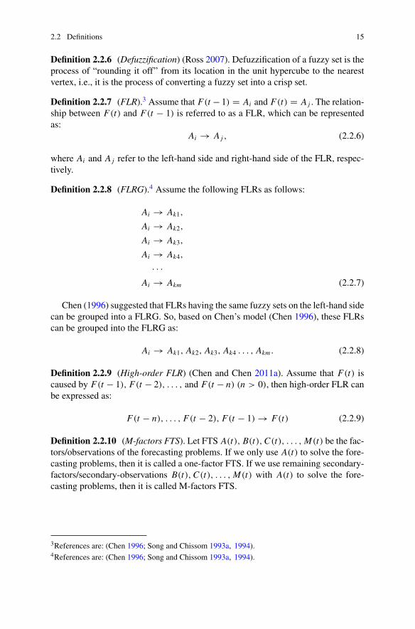
Definition 2.2.7 (FLR).3 Assume that F(t − 1) = Ai and F(t) = A j . The relation-ship between F(t) and F(t − 1) is referred to as a FLR, which can be representedas:

Ai → A j , (2.2.6)

where Ai and A j refer to the left-hand side and right-hand side of the FLR, respec-tively.

Definition 2.2.8 (FLRG).4 Assume the following FLRs as follows:

Ai → Ak1,

Ai → Ak2,

Ai → Ak3,

Ai → Ak4,

· · ·Ai → Akm (2.2.7)

Chen (1996) suggested that FLRs having the same fuzzy sets on the left-hand sidecan be grouped into a FLRG. So, based on Chen’s model (Chen 1996), these FLRscan be grouped into the FLRG as:

Ai → Ak1, Ak2, Ak3, Ak4 . . . , Akm . (2.2.8)

Definition 2.2.9 (High-order FLR) (Chen and Chen 2011a). Assume that F(t) iscaused by F(t − 1), F(t − 2), . . . , and F(t − n) (n > 0), then high-order FLR canbe expressed as:

F(t − n), . . . , F(t − 2), F(t − 1) → F(t) (2.2.9)

Definition 2.2.10 (M-factors FTS). Let FTS A(t), B(t), C(t), . . . , M(t) be the fac-tors/observations of the forecasting problems. If we only use A(t) to solve the fore-casting problems, then it is called a one-factor FTS. If we use remaining secondary-factors/secondary-observations B(t), C(t), . . . , M(t) with A(t) to solve the fore-casting problems, then it is called M-factors FTS.

3References are: (Chen 1996; Song and Chissom 1993a, 1994).4References are: (Chen 1996; Song and Chissom 1993a, 1994).


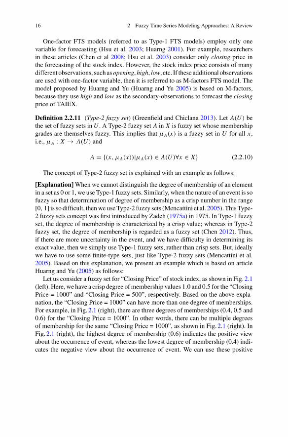
One-factor FTS models (referred to as Type-1 FTS models) employ only onevariable for forecasting (Hsu et al. 2003; Huarng 2001). For example, researchersin these articles (Chen et al 2008; Hsu et al. 2003) consider only closing price inthe forecasting of the stock index. However, the stock index price consists of manydifferent observations, such asopening,high, low, etc. If these additional observationsare used with one-factor variable, then it is referred to as M-factors FTS model. Themodel proposed by Huarng and Yu (Huarng and Yu 2005) is based on M-factors,because they use high and low as the secondary-observations to forecast the closingprice of TAIEX.

Definition 2.2.11 (Type-2 fuzzy set) (Greenfield and Chiclana 2013). Let A(U ) bethe set of fuzzy sets in U . A Type-2 fuzzy set A in X is fuzzy set whose membershipgrades are themselves fuzzy. This implies that μA(x) is a fuzzy set in U for all x ,i.e., μA : X → A(U ) and

A = {(x, μA(x))|μA(x) ∈ A(U )∀x ∈ X} (2.2.10)

The concept of Type-2 fuzzy set is explained with an example as follows:

[Explanation] When we cannot distinguish the degree of membership of an elementin a set as 0 or 1, we use Type-1 fuzzy sets. Similarly, when the nature of an event is sofuzzy so that determination of degree of membership as a crisp number in the range[0, 1] is so difficult, thenwe use Type-2 fuzzy sets (Mencattini et al. 2005). This Type-2 fuzzy sets concept was first introduced by Zadeh (1975a) in 1975. In Type-1 fuzzyset, the degree of membership is characterized by a crisp value; whereas in Type-2fuzzy set, the degree of membership is regarded as a fuzzy set (Chen 2012). Thus,if there are more uncertainty in the event, and we have difficulty in determining itsexact value, then we simply use Type-1 fuzzy sets, rather than crisp sets. But, ideallywe have to use some finite-type sets, just like Type-2 fuzzy sets (Mencattini et al.2005). Based on this explanation, we present an example which is based on articleHuarng and Yu (2005) as follows:

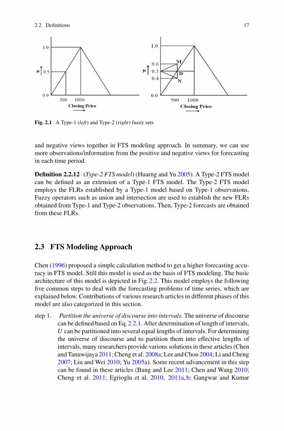
Let us consider a fuzzy set for “Closing Price” of stock index, as shown in Fig. 2.1(left). Here, we have a crisp degree ofmembership values 1.0 and 0.5 for the “ClosingPrice = 1000” and “Closing Price = 500”, respectively. Based on the above expla-nation, the “Closing Price = 1000” can have more than one degree of memberships.For example, in Fig. 2.1 (right), there are three degrees of memberships (0.4, 0.5 and0.6) for the “Closing Price = 1000”. In other words, there can be multiple degreesof membership for the same “Closing Price = 1000”, as shown in Fig. 2.1 (right). InFig. 2.1 (right), the highest degree of membership (0.6) indicates the positive viewabout the occurrence of event, whereas the lowest degree of membership (0.4) indi-cates the negative view about the occurrence of event. We can use these positive

2.2 Definitions 17

Fig. 2.1 A Type-1 (left) and Type-2 (right) fuzzy sets

and negative views together in FTS modeling approach. In summary, we can usemore observations/information from the positive and negative views for forecastingin each time period.

Definition 2.2.12 (Type-2 FTS model) (Huarng and Yu 2005). A Type-2 FTS modelcan be defined as an extension of a Type-1 FTS model. The Type-2 FTS modelemploys the FLRs established by a Type-1 model based on Type-1 observations.Fuzzy operators such as union and intersection are used to establish the new FLRsobtained from Type-1 and Type-2 observations. Then, Type-2 forecasts are obtainedfrom these FLRs.

2.3 FTS Modeling Approach

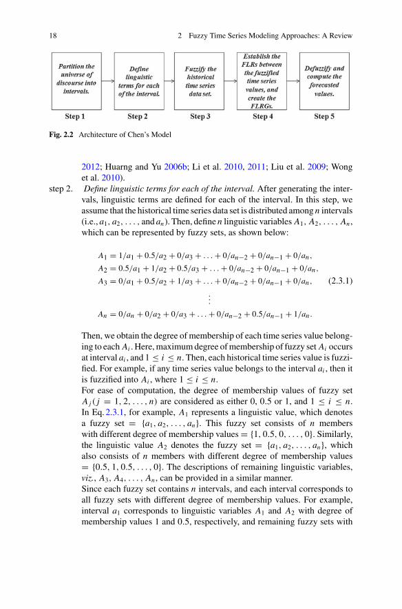
Chen (1996) proposed a simple calculation method to get a higher forecasting accu-racy in FTS model. Still this model is used as the basis of FTS modeling. The basicarchitecture of this model is depicted in Fig. 2.2. This model employs the followingfive common steps to deal with the forecasting problems of time series, which areexplained below. Contributions of various research articles in different phases of thismodel are also categorized in this section.

step 1. Partition the universe of discourse into intervals. The universe of discoursecan be defined based on Eq.2.2.1. After determination of length of intervals,U can be partitioned into several equal lengths of intervals. For determiningthe universe of discourse and to partition them into effective lengths ofintervals, many researchers provide various solutions in these articles (ChenandTanuwijaya 2011;Cheng et al. 2008a; Lee andChou 2004; Li andCheng2007; Liu and Wei 2010; Yu 2005a). Some recent advancement in this stepcan be found in these articles (Bang and Lee 2011; Chen and Wang 2010;Cheng et al. 2011; Egrioglu et al. 2010, 2011a, b; Gangwar and Kumar


Fig. 2.2 Architecture of Chen’s Model

2012; Huarng and Yu 2006b; Li et al. 2010, 2011; Liu et al. 2009; Wonget al. 2010).

step 2. Define linguistic terms for each of the interval. After generating the inter-vals, linguistic terms are defined for each of the interval. In this step, weassume that the historical time series data set is distributed among n intervals(i.e., a1, a2, . . . , and an). Then, define n linguistic variables A1, A2, . . . , An ,which can be represented by fuzzy sets, as shown below:

A1 = 1/a1 + 0.5/a2 + 0/a3 + . . . + 0/an−2 + 0/an−1 + 0/an,

A2 = 0.5/a1 + 1/a2 + 0.5/a3 + . . . + 0/an−2 + 0/an−1 + 0/an,

A3 = 0/a1 + 0.5/a2 + 1/a3 + . . . + 0/an−2 + 0/an−1 + 0/an, (2.3.1)

...

An = 0/an + 0/a2 + 0/a3 + . . . + 0/an−2 + 0.5/an−1 + 1/an .

Then, we obtain the degree of membership of each time series value belong-ing to each Ai . Here,maximumdegree ofmembership of fuzzy set Ai occursat interval ai , and 1 ≤ i ≤ n. Then, each historical time series value is fuzzi-fied. For example, if any time series value belongs to the interval ai , then itis fuzzified into Ai , where 1 ≤ i ≤ n.For ease of computation, the degree of membership values of fuzzy setA j ( j = 1, 2, . . . , n) are considered as either 0, 0.5 or 1, and 1 ≤ i ≤ n.In Eq.2.3.1, for example, A1 represents a linguistic value, which denotesa fuzzy set = {a1, a2, . . . , an}. This fuzzy set consists of n memberswith different degree of membership values = {1, 0.5, 0, . . . , 0}. Similarly,the linguistic value A2 denotes the fuzzy set = {a1, a2, . . . , an}, whichalso consists of n members with different degree of membership values= {0.5, 1, 0.5, . . . , 0}. The descriptions of remaining linguistic variables,viz., A3, A4, . . . , An , can be provided in a similar manner.Since each fuzzy set contains n intervals, and each interval corresponds toall fuzzy sets with different degree of membership values. For example,interval a1 corresponds to linguistic variables A1 and A2 with degree ofmembership values 1 and 0.5, respectively, and remaining fuzzy sets with

2.3 FTS Modeling Approach 19

degree of membership value 0. Similarly, interval a2 corresponds to lin-guistic variables A1, A2 and A3 with degree of membership values 0.5, 1,and 0.5, respectively, and remaining fuzzy sets with degree of membershipvalue 0. The descriptions of remaining intervals, viz., a3, a4, . . . , an , can beprovided in a similar manner.Liu (2007) introduced an improved FTS forecasting method in which theforecasted value is regarded as a trapezoidal fuzzy number instead of asingle-point value. They replace the above discrete fuzzy sets (as discussedin Eq.2.3.1) with trapezoidal fuzzy numbers. The main advantage of theproposed method is that the decision analyst can accumulate informationabout the possible forecasted ranges under different degrees of confidence.

step 3. Fuzzify the historical time series data set. In order to fuzzify the historicaltime series data, it is essential to obtain the degree of membership value ofeach observation belonging to each A j ( j = 1, 2, . . . , n) for each day/year.If the maximum membership value of one day’s/year’s observation occursat interval ai and 1 ≤ i ≤ n, then the fuzzified value for that particularday/year is considered as Ai .In FTS model, each fuzzy set carries the information of occurrence of thehistoric event in the past. So, if these fuzzy sets would not be handled effi-ciently, then important information may be lost. Therefore, for fuzzificationpurpose, many researchers provided different techniques in these articles(Cheng et al. 2006; Hwang et al. 1998; Sah and Degtiarev 2005).

step 4. Establish the FLRs between the fuzzified time series values, and create theFLRGs. After time series data is completely fuzzified, then FLRs have beenestablished based on Definition 2.2.7. The first-order FLR is establishedbased on two consecutive linguistic values. For example, if the fuzzifiedvalues of time t − 1 and t are Ai and A j , respectively, then establish thefirst-order FLR as “Ai → A j”, where “Ai” and “A j” are called the previousstate and current state of the FLR, respectively. Similarly, the nth-order FLRis established based on n + 1 consecutive linguistic values. For example, ifthe fuzzified values of time t − 4, t − 3, t − 2, t − 1 and t are Aai , Abi ,Aci , Adi and Aej , respectively, then the fourth-order FLR can be establishedas “Aai , Abi , Aci , Adi → Aej”, where “Aai , Abi , Aci , Adi” and “Aej” arecalled the previous state nd current state of the FLR, respectively.Most of the existing FTS models5 use the first-order FLRs to get the fore-casting results. In these articles,6 researchers show that the high-order FLRs(see Definition 2.2.9) can improve the forecasting accuracy. The main rea-son of obtaining high accuracy from these high-order FTS models is thatit can consider more linguistic values that represent the high uncertainty

5References are: (Chang et al. 2007; Chen 1996; Cheng et al. 2006; Huarng 2001; Hwang et al.1998; Song and Chissom 1993a,b, 1994).6References are: (Aladag et al. 2009, 2010; Avazbeigi et al. 2010; Bahrepour et al. 2011; Chen2002; Chen and Chen 2011a, b; Chen and Chung 2006b; Chen et al 2008; Gangwar and Kumar2012; Jilani and Burney 2008; Own and Yu 2005; Singh 2007a, c, 2008, 2009; Tsai and Wu 2000).


involved in various dynamic processes. On the other hand, to extract rulefrom the fuzzified time series data set, Qiu et al. (2012) utilized C-fuzzydecision trees (Pedrycz and Sosnowski 2005) in FTS model. They intro-duced two major improvements in C-fuzzy decision trees, viz., first a newstop condition is introduced to reduce the computational cost, and secondweighted C-fuzzy decision tree (WCDT) is introduced where weight dis-tance is computed with information gain. In this approach, the forecast ruleare expressed as “if input value is . . . then it can be labeled as . . .”.Based on the same previous state of the FLRs, the FLRs can be grouped intoa FLRG (see Definition 2.2.8). For example, the FLRG “Ai → Am, An”indicates that there are following FLRs:

Ai → Am,

Ai → An.

Step 5. Defuzzify and compute the forecasted values. In these articles (Song andChissom 1993a; Tsaur et al. 2005), researchers adopted the followingmethod to forecast enrollments of the University of Alabama:

Y (t) = Y (t − 1) ◦ R, (2.3.2)

where Y (t − 1) is the fuzzified enrollment of year (t − 1), Y (t) is theforecasted enrollment of year t represented by fuzzy set, “◦” is the max-mincomposition operator, and “R” is the union of fuzzy relations. This methodtakes much time to compute the union of fuzzy relations R, especiallywhen the number of fuzzy relations is more in Eq.2.3.2 (Chen and Hwang2000; Huarng et al 2007). Therefore, some researchers in these articles7

introduced various solutions for the defuzzification operation. One of thesolution introduced by Chen (Chen 1996) is presented below.This includes the following two principles, viz., Principle 1 and Principle2. The procedure for Principle 1 is given as follows:

• Principle 1: For forecasting F(t), the fuzzified value for F(t−1) is required,where“t” is the current time which we want to forecast. The Principle 1 is applicableonly if there are more than one fuzzified values available in the current state. Thesteps under Principle 1 are explained next.

Step 1. Obtain the fuzzified value for F(t − 1) as Ai (i = 1, 2, 3 . . . , n).Step 2. Obtain the FLR whose previous state is Ai and the current state is

A j1, A j2, . . . , A jp, i.e., the FLR is in the form of “Ai → A j1, A j2,

. . . , A jp”.

7References are: (Chen 1996, 2002; Cheng et al. 2008b; Huarng 2001; Huarng et al 2007; Hwanget al. 1998; Jilani and Burney 2008; Kuo et al. 2009; Lee et al. 2006; Li et al. 2008; Qiu et al 2011;Singh and Borah 2012, 2013b; Singh 2007a, b, 2009; Yu 2005b).

2.3 FTS Modeling Approach 21

Step 3. Find the interval where the maximum membership value of the fuzzysets A j1, A j2, . . . , A jp (current state) occur, and let these intervals bea j1, a j2, . . . , a jp. All these intervals have the corresponding mid-valuesC j1, C j2, . . . , C jp.

Step 3. Compute the forecasted value as:

Forecastedvalue =[

C j1 + C j2 + . . . + C jp

p

](2.3.3)

Here, p represents the total number of fuzzy sets associatedwith the currentstate of the FLR.

• Principle 2: This principle is applicable only if there is only one fuzzified valuein the current state. The steps under Principle 2 are given as follows:

Step 1. Obtain the fuzzified value for F(t − 1) as Ai (i = 1, 2, . . . , n).Step 2. Find the FLR whose previous state is Ai and the current state is A j , i.e.,

the FLR is in the form of “Ai → A j”.Step 3. Find the interval where the maximum membership value of the fuzzy set

A j occurs. Let these interval be a j ( j = 1, 2, 3, . . . , n). This interval a j

has the corresponding mid-value C j . This C j is the forecasted value forF(t).

2.4 Hybridize Modeling Approach for FTS

Recently, several SC techniques have been employed to deal with the different chal-lenges imposed by the FTS modeling approach. The main SC techniques for thispurpose include ANN, RS, and EC. Each of them provides significant solution foraddressing domain specific problems. The combination of these techniques leads tothe development of new architecture, which is more advantageous and the expert,providing robust, cost effective and approximate solution, in comparison to conven-tional techniques. However, this hybridization should be carried out in a reasonable,rather than an expensive or a complicated, manner.

In the following, we describe the basics of individual SC techniques and theirhybridization techniques, along with the several hybridized models developed forhandling forecasting problems of the FTS modeling approach. It should be notedthat still there is no any universally recognized method to select particular SC tech-nique(s), which is suitable for resolving the problems. The selection of technique(s)is completely dependent on the problem and its application, and requires humaninterpretation for determining the suitability of a particular technique.


2.4.1 ANN: An Introduction

ANNs are massively parallel adaptive networks of simple nonlinear computing ele-ments called neurons which are intended to abstract and model some of the func-tionality of the human nervous system in an attempt to partially capture some of itscomputational strengths (Kumar 2004). The neurons in an ANN are organized intodifferent layers. Inputs to the network are entered in the input layer; whereas outputsare produced as signals in the output layer. These signals may pass through one ormore intermediate or hidden layers which transform the signals depending upon theneuron signal functions.

The neural networks are classified into either single-layer or multi-layer. In multi-layer networks hidden layers exist between input layer and output layer. A single-layer feed-forward (SLFF) neural network is formed when the nodes of input layerare connected with output nodes with various weights. A multi-layer feed-forward(MLFF) neural network architecture can be developed by increasing the number oflayers in SLFF neural network. Feed-forward ANNs allow signals to travel frominput to output. There is no feed-back loop. Feed-back networks can have signalstravelling in both directions by introducing loops in the network. Feed-back networksare also referred to as interactive or recurrent networks.

Usually FFNN are used in time series forecasting. Recurrent networks are alsoused in some cases. Researchers employ ANN in various forecasting problems suchas electric load forecasting (Taylor and Buizza 2002), short-term precipitation fore-casting (Kuligowski and Barros 1998), credit ratings forecasting (Kumar and Bhat-tacharya 2006), tourism demand forecasting (Law 2000) etc., due to its capabilityto discover complex nonlinear relationships (Czibula et al. 2013; Donaldson andKamstra 1996; Indro et al. 1999) in the observations. More detailed description onapplications of ANN (especially BPNN) can be found in article written by Wilsonet al. (2002).

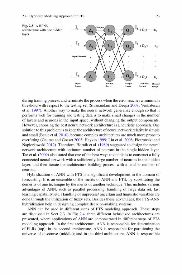
Multi-layer FFNN uses back-propagation learning algorithm, therefore such net-works are also known as back-propagation networks (BPNN). The main objective ofusing BPNN is to minimize the output error obtained from the difference betweenthe calculated output (o1, o2, . . . , on) and target output (n1, n2, . . . , nn) of the neuralnetwork by adjusting the weights (see Fig. 2.3). So in BPNN, each information issent back again in the reverse direction until the output error is very small or zero.BPNN is trained under the process of three phases: (a) feed-forward of the inputtraining pattern, (b) the calculation and back-propagation of the associated error, and(c) the adjustment of the weights.

Due to large number of additional parameters (e.g., initial weight, learning rate,momentum, epoch, activation function, etc.), an ANN model has great capabilityto learn by making proper adjustment of these parameters, in order to produce thedesired output. During the training process, this output may fit the data very well,but it may produce poor results during the testing process. This implies that theneural network may not generalize well. This might be caused due to overfitting orovertraining of data (Weigend 1994), which can be controlled bymonitoring the error

2.4 Hybridize Modeling Approach for FTS 23

Fig. 2.3 A BPNNarchitecture with one hiddenlayer

during training process and terminate the process when the error reaches a minimumthreshold with respect to the testing set (Sivanandam and Deepa 2007; Venkatesanet al. 1997). Another way to make the neural network generalize enough so that itperforms well for training and testing data is to make small changes in the numberof layers and neurons in the input space, without changing the output components.However, choosing the best neural network architecture is a heuristic approach. Onesolution to this problem is to keep the architecture of neural network relatively simpleand small (Beale et al. 2010), because complex architectures are much more prone tooverfitting (Gaume and Gosset 2003; Haykin 1999; Liu et al. 2008; Piotrowski andNapiorkowski 2012). Therefore, Hornik et al. (1989) suggested to design the neuralnetwork architecture with optimum number of neurons in the single hidden layer.Tan et al. (2009) also stated that one of the best ways to do this is to construct a fullyconnected neural network with a sufficiently large number of neurons in the hiddenlayer, and then iterate the architecture-building process with a smaller number ofneurons.

Hybridization of ANN with FTS is a significant development in the domain offorecasting. It is an ensemble of the merits of ANN and FTS, by substituting thedemerits of one technique by the merits of another technique. This includes variousadvantages of ANN, such as parallel processing, handling of large data set, fastlearning capability, etc. Handling of imprecise/ uncertain and linguistic variables aredone through the utilization of fuzzy sets. Besides these advantages, the FTS-ANNhybridization help in designing complex decision-making systems.

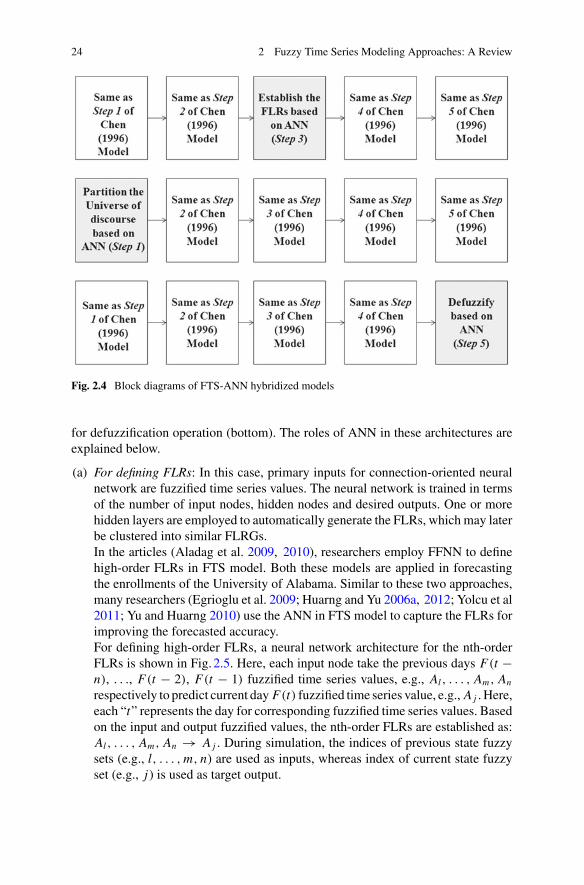
ANN can be used in different steps of FTS modeling approach. These stepsare discussed in Sect. 2.3. In Fig. 2.4, three different hybridized architectures arepresented, where applications of ANN are demonstrated in different steps of FTSmodeling approach. In the first architecture, ANN is responsible for determinationof FLRs (top); in the second architecture, ANN is responsible for partitioning theuniverse of discourse (middle); and in the third architecture, ANN is responsible


Fig. 2.4 Block diagrams of FTS-ANN hybridized models

for defuzzification operation (bottom). The roles of ANN in these architectures areexplained below.

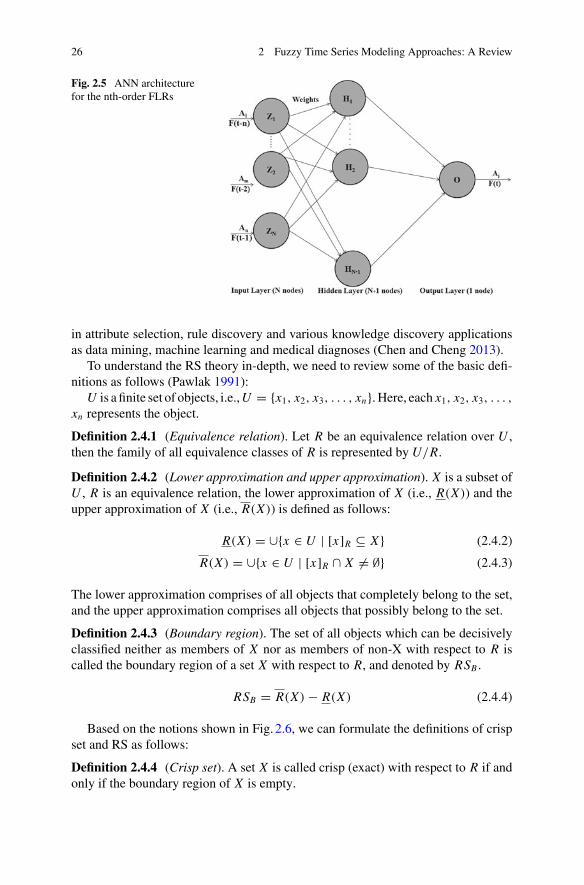
(a) For defining FLRs: In this case, primary inputs for connection-oriented neuralnetwork are fuzzified time series values. The neural network is trained in termsof the number of input nodes, hidden nodes and desired outputs. One or morehidden layers are employed to automatically generate the FLRs, which may laterbe clustered into similar FLRGs.In the articles (Aladag et al. 2009, 2010), researchers employ FFNN to definehigh-order FLRs in FTS model. Both these models are applied in forecastingthe enrollments of the University of Alabama. Similar to these two approaches,many researchers (Egrioglu et al. 2009; Huarng and Yu 2006a, 2012; Yolcu et al2011; Yu and Huarng 2010) use the ANN in FTS model to capture the FLRs forimproving the forecasted accuracy.For defining high-order FLRs, a neural network architecture for the nth-orderFLRs is shown in Fig. 2.5. Here, each input node take the previous days F(t −n), . . ., F(t − 2), F(t − 1) fuzzified time series values, e.g., Al, . . . , Am, An

respectively to predict current day F(t) fuzzified time series value, e.g., A j . Here,each “t” represents the day for corresponding fuzzified time series values. Basedon the input and output fuzzified values, the nth-order FLRs are established as:Al, . . . , Am, An → A j . During simulation, the indices of previous state fuzzysets (e.g., l, . . . , m, n) are used as inputs, whereas index of current state fuzzyset (e.g., j) is used as target output.


(b) For partitioning the Universe of discourse: Data clustering is a popular approachfor automatically finding classes, concepts, or groups of patterns (Gondek andHofmann 2007). Time series data are pervasive across all human endeavors,and their clustering is one of the most fundamental applications of data mining(Keogh and Lin 2005). In literature, many data clustering algorithms (Estivill-Castro 2002; Ordonez 2003; Wu et al. 2008) have been proposed, but theirapplications are limited to the extraction of patterns that represent points in mul-tidimensional spaces of fixed dimensionality (Xiong and Yeung 2002). In thesearticles (Bahrepour et al. 2011; Singh and Borah 2012), researchers employSOFM clustering algorithm for determining the intervals of the historical timeseries data sets by clustering them into different groups. This algorithm is devel-oped by Kohonen (Kohonen 1990), which is a class of neural networks withneurons arranged in a low dimensional (often two-dimensional) structure, andtrained by an iterative unsupervised or self-organizing procedure (Liao 2005).The SOFM converts the patterns of arbitrary dimensionality into response ofone-dimensional or two-dimensional arrays of neurons, i.e., it converts a widepattern space into a feature space. The neural network performing such a map-ping is called feature map (Sivanandam and Deepa 2007).

(c) For defuzzification operation: (Singh and Borah (2013b) develop an ANN basedarchitecture and hybridize this architecture with FTS model to defuzzify thefuzzified time series values. The neural network architecture as shown in Fig. 2.5can be employed for this purpose. In this case, the arrangement of nodes in inputlayer can be done in the following sequence:

F(t − n), . . . , F(t − 2), F(t − 1) → F(t) (2.4.1)

Here, each input node take the previous days (t −n), . . . , (t −2), (t −1) fuzzifiedtime series values (e.g., Al , . . . , Am, An) to predict one day (t) advance timeseries value “A j”. In Eq.2.4.1, each “t” represent the day for considered fuzzifiedtime series values.

2.4.2 RS: An Introduction

RS is a new mathematical tool proposed by Pawlak (Pawlak 1982). The RS concept(Cheng et al. 2010) is based on the assumption that with every associated objectof the universe of discourse, some information objects characterized by the sameinformation are indiscernible in the view of the available information about them.Any set of all indiscernible objects is called an elementary set and forms a basicgranule of knowledge about the universe. Any union of elementary sets is referredto as a precise set; otherwise the set is rough. A fundamental advantage of RStheory is the ability to handle a category that cannot be sharply defined from a givenknowledge base (Pattaraintakorn andCercone 2008). Therefore, theRS theory is used


Fig. 2.5 ANN architecturefor the nth-order FLRs

in attribute selection, rule discovery and various knowledge discovery applicationsas data mining, machine learning and medical diagnoses (Chen and Cheng 2013).

To understand the RS theory in-depth, we need to review some of the basic defi-nitions as follows (Pawlak 1991):

U is a finite set of objects, i.e.,U = {x1, x2, x3, . . . , xn}. Here, each x1, x2, x3, . . . ,xn represents the object.

Definition 2.4.1 (Equivalence relation). Let R be an equivalence relation over U ,then the family of all equivalence classes of R is represented by U/R.

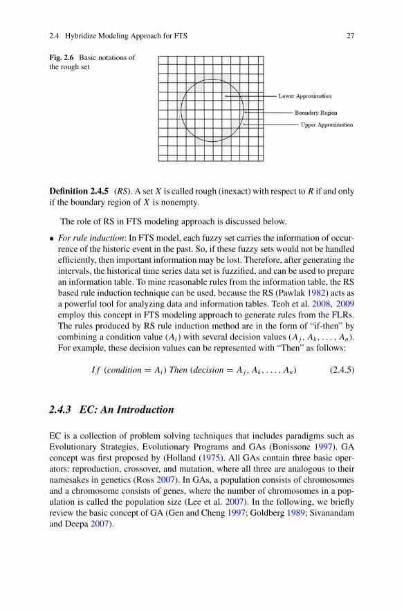
Definition 2.4.2 (Lower approximation and upper approximation). X is a subset ofU , R is an equivalence relation, the lower approximation of X (i.e., R(X)) and theupper approximation of X (i.e., R(X)) is defined as follows:

R(X) = ∪{x ∈ U | [x]R ⊆ X} (2.4.2)

R(X) = ∪{x ∈ U | [x]R ∩ X = ∅} (2.4.3)

The lower approximation comprises of all objects that completely belong to the set,and the upper approximation comprises all objects that possibly belong to the set.

Definition 2.4.3 (Boundary region). The set of all objects which can be decisivelyclassified neither as members of X nor as members of non-X with respect to R iscalled the boundary region of a set X with respect to R, and denoted by RSB .

RSB = R(X) − R(X) (2.4.4)

Based on the notions shown in Fig. 2.6, we can formulate the definitions of crispset and RS as follows:

Definition 2.4.4 (Crisp set). A set X is called crisp (exact) with respect to R if andonly if the boundary region of X is empty.


Fig. 2.6 Basic notations ofthe rough set

Definition 2.4.5 (RS). A set X is called rough (inexact) with respect to R if and onlyif the boundary region of X is nonempty.

The role of RS in FTS modeling approach is discussed below.

• For rule induction: In FTS model, each fuzzy set carries the information of occur-rence of the historic event in the past. So, if these fuzzy sets would not be handledefficiently, then important information may be lost. Therefore, after generating theintervals, the historical time series data set is fuzzified, and can be used to preparean information table. To mine reasonable rules from the information table, the RSbased rule induction technique can be used, because the RS (Pawlak 1982) acts asa powerful tool for analyzing data and information tables. Teoh et al. 2008, 2009employ this concept in FTS modeling approach to generate rules from the FLRs.The rules produced by RS rule induction method are in the form of “if-then” bycombining a condition value (Ai ) with several decision values (A j , Ak, . . . , An).For example, these decision values can be represented with “Then” as follows:

I f (condition = Ai ) Then (decision = A j , Ak, . . . , An) (2.4.5)

2.4.3 EC: An Introduction

EC is a collection of problem solving techniques that includes paradigms such asEvolutionary Strategies, Evolutionary Programs and GAs (Bonissone 1997). GAconcept was first proposed by (Holland (1975). All GAs contain three basic oper-ators: reproduction, crossover, and mutation, where all three are analogous to theirnamesakes in genetics (Ross 2007). In GAs, a population consists of chromosomesand a chromosome consists of genes, where the number of chromosomes in a pop-ulation is called the population size (Lee et al. 2007). In the following, we brieflyreview the basic concept of GA (Gen and Cheng 1997; Goldberg 1989; Sivanandamand Deepa 2007).


Step 1. Create a random initial state. An initial population is created from a ran-dom selection of solutions (chromosomes).

Step 2. Evaluate fitness. A value for fitness is assigned to each solution dependingon how close it actually is to solving the problem.

Step 3. Reproduce. Those chromosomes with a higher fitness value aremore likelyto reproduce offspring.

Step 4. Next generation. If the new generation contains a solution that producesan output that is close enough or equal to the desired answer then theproblem has been solved. Otherwise, iterate the whole process with thenew generation.

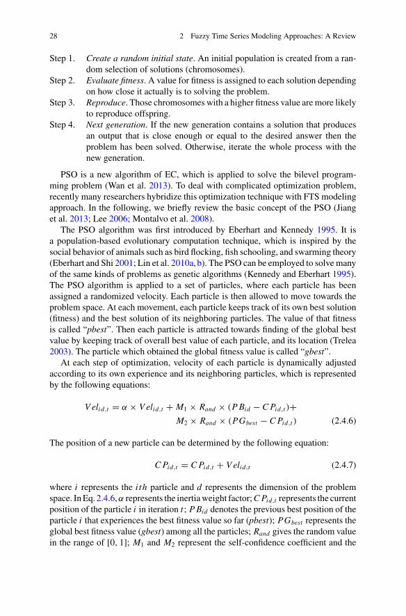
PSO is a new algorithm of EC, which is applied to solve the bilevel program-ming problem (Wan et al. 2013). To deal with complicated optimization problem,recently many researchers hybridize this optimization technique with FTS modelingapproach. In the following, we briefly review the basic concept of the PSO (Jianget al. 2013; Lee 2006; Montalvo et al. 2008).

The PSO algorithm was first introduced by Eberhart and Kennedy 1995. It isa population-based evolutionary computation technique, which is inspired by thesocial behavior of animals such as bird flocking, fish schooling, and swarming theory(Eberhart and Shi 2001; Lin et al. 2010a, b). The PSO can be employed to solve manyof the same kinds of problems as genetic algorithms (Kennedy and Eberhart 1995).The PSO algorithm is applied to a set of particles, where each particle has beenassigned a randomized velocity. Each particle is then allowed to move towards theproblem space. At each movement, each particle keeps track of its own best solution(fitness) and the best solution of its neighboring particles. The value of that fitnessis called “pbest”. Then each particle is attracted towards finding of the global bestvalue by keeping track of overall best value of each particle, and its location (Trelea2003). The particle which obtained the global fitness value is called “gbest”.

At each step of optimization, velocity of each particle is dynamically adjustedaccording to its own experience and its neighboring particles, which is representedby the following equations:

V elid,t = α × V elid,t + M1 × Rand × (P Bid − C Pid,t )+M2 × Rand × (PGbest − C Pid,t ) (2.4.6)

The position of a new particle can be determined by the following equation:

C Pid,t = C Pid,t + V elid,t (2.4.7)

where i represents the i th particle and d represents the dimension of the problemspace. InEq.2.4.6,α represents the inertiaweight factor;C Pid,t represents the currentposition of the particle i in iteration t ; P Bid denotes the previous best position of theparticle i that experiences the best fitness value so far (pbest); PGbest represents theglobal best fitness value (gbest) among all the particles; Rand gives the random valuein the range of [0, 1]; M1 and M2 represent the self-confidence coefficient and the


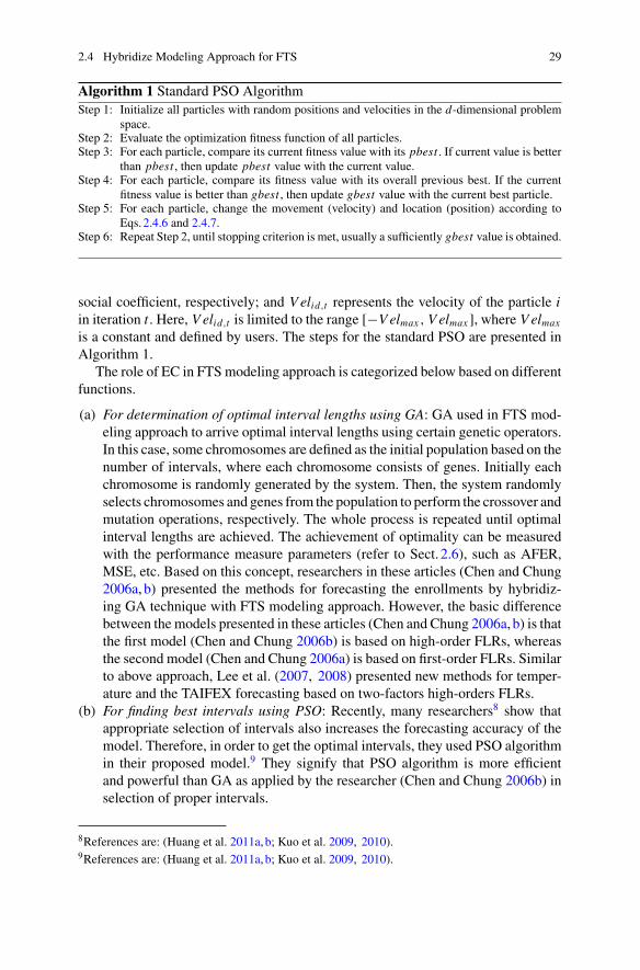
Algorithm 1 Standard PSO AlgorithmStep 1: Initialize all particles with random positions and velocities in the d-dimensional problem

space.Step 2: Evaluate the optimization fitness function of all particles.Step 3: For each particle, compare its current fitness value with its pbest . If current value is better

than pbest , then update pbest value with the current value.Step 4: For each particle, compare its fitness value with its overall previous best. If the current

fitness value is better than gbest , then update gbest value with the current best particle.Step 5: For each particle, change the movement (velocity) and location (position) according to

Eqs. 2.4.6 and 2.4.7.Step 6: Repeat Step 2, until stopping criterion is met, usually a sufficiently gbest value is obtained.

social coefficient, respectively; and V elid,t represents the velocity of the particle iin iteration t . Here, V elid,t is limited to the range [−V elmax , V elmax ], where V elmax

is a constant and defined by users. The steps for the standard PSO are presented inAlgorithm 1.

The role of EC in FTSmodeling approach is categorized below based on differentfunctions.

(a) For determination of optimal interval lengths using GA: GA used in FTS mod-eling approach to arrive optimal interval lengths using certain genetic operators.In this case, some chromosomes are defined as the initial population based on thenumber of intervals, where each chromosome consists of genes. Initially eachchromosome is randomly generated by the system. Then, the system randomlyselects chromosomes and genes from the population to perform the crossover andmutation operations, respectively. The whole process is repeated until optimalinterval lengths are achieved. The achievement of optimality can be measuredwith the performance measure parameters (refer to Sect. 2.6), such as AFER,MSE, etc. Based on this concept, researchers in these articles (Chen and Chung2006a, b) presented the methods for forecasting the enrollments by hybridiz-ing GA technique with FTS modeling approach. However, the basic differencebetween the models presented in these articles (Chen and Chung 2006a, b) is thatthe first model (Chen and Chung 2006b) is based on high-order FLRs, whereasthe second model (Chen and Chung 2006a) is based on first-order FLRs. Similarto above approach, Lee et al. (2007, 2008) presented new methods for temper-ature and the TAIFEX forecasting based on two-factors high-orders FLRs.

(b) For finding best intervals using PSO: Recently, many researchers8 show thatappropriate selection of intervals also increases the forecasting accuracy of themodel. Therefore, in order to get the optimal intervals, they used PSO algorithmin their proposed model.9 They signify that PSO algorithm is more efficientand powerful than GA as applied by the researcher (Chen and Chung 2006b) inselection of proper intervals.

8References are: (Huang et al. 2011a, b; Kuo et al. 2009, 2010).9References are: (Huang et al. 2011a, b; Kuo et al. 2009, 2010).


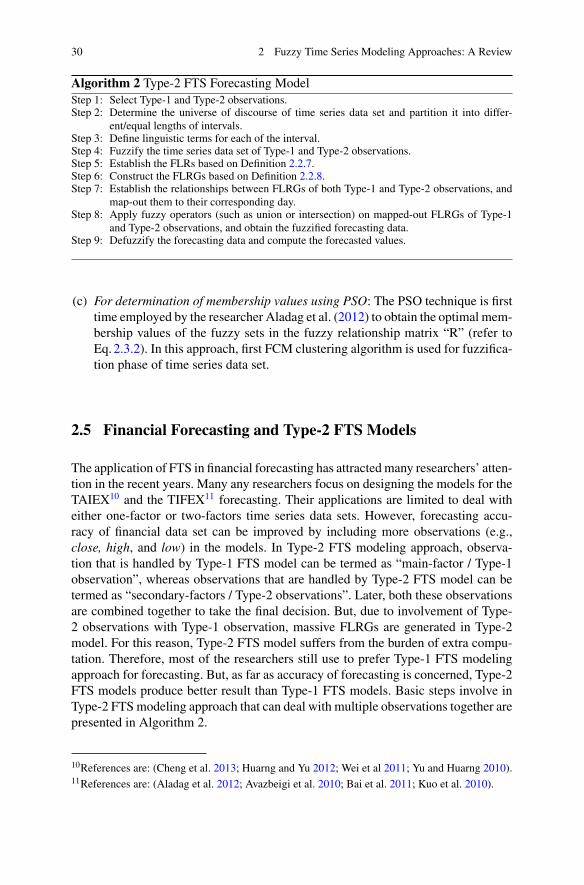
Algorithm 2 Type-2 FTS Forecasting ModelStep 1: Select Type-1 and Type-2 observations.Step 2: Determine the universe of discourse of time series data set and partition it into differ-

ent/equal lengths of intervals.Step 3: Define linguistic terms for each of the interval.Step 4: Fuzzify the time series data set of Type-1 and Type-2 observations.Step 5: Establish the FLRs based on Definition 2.2.7.Step 6: Construct the FLRGs based on Definition 2.2.8.Step 7: Establish the relationships between FLRGs of both Type-1 and Type-2 observations, and

map-out them to their corresponding day.Step 8: Apply fuzzy operators (such as union or intersection) on mapped-out FLRGs of Type-1

and Type-2 observations, and obtain the fuzzified forecasting data.Step 9: Defuzzify the forecasting data and compute the forecasted values.

(c) For determination of membership values using PSO: The PSO technique is firsttime employed by the researcher Aladag et al. (2012) to obtain the optimal mem-bership values of the fuzzy sets in the fuzzy relationship matrix “R” (refer toEq.2.3.2). In this approach, first FCM clustering algorithm is used for fuzzifica-tion phase of time series data set.

2.5 Financial Forecasting and Type-2 FTS Models

The application of FTS in financial forecasting has attractedmany researchers’ atten-tion in the recent years. Many any researchers focus on designing the models for theTAIEX10 and the TIFEX11 forecasting. Their applications are limited to deal witheither one-factor or two-factors time series data sets. However, forecasting accu-racy of financial data set can be improved by including more observations (e.g.,close, high, and low) in the models. In Type-2 FTS modeling approach, observa-tion that is handled by Type-1 FTS model can be termed as “main-factor / Type-1observation”, whereas observations that are handled by Type-2 FTS model can betermed as “secondary-factors / Type-2 observations”. Later, both these observationsare combined together to take the final decision. But, due to involvement of Type-2 observations with Type-1 observation, massive FLRGs are generated in Type-2model. For this reason, Type-2 FTS model suffers from the burden of extra compu-tation. Therefore, most of the researchers still use to prefer Type-1 FTS modelingapproach for forecasting. But, as far as accuracy of forecasting is concerned, Type-2FTS models produce better result than Type-1 FTS models. Basic steps involve inType-2 FTSmodeling approach that can deal with multiple observations together arepresented in Algorithm 2.

10References are: (Cheng et al. 2013; Huarng and Yu 2012; Wei et al 2011; Yu and Huarng 2010).11References are: (Aladag et al. 2012; Avazbeigi et al. 2010; Bai et al. 2011; Kuo et al. 2010).

2.5 Financial Forecasting and Type-2 FTS Models 31

Contributions of various researchers in Type-2 FTS models are presented below:

• Huarng and Yu (Huarng and Yu 2005) model: This model first time employs theType-2 FTS concept in financial forecasting (TAIEX) by considering close, high,and low observations together. In this model, they suggested some improvementin Algorithm 2 as:(i) Introduction of union (∨) and intersection (∧) operators. This operators areapplied in Step 8 of Algorithm 2. Both these operators are used to include Type-1 and Type-2 observations., and (ii) For defuzzification operation, they employPrincipal 1 and Principal 2 (as discussed in Sect. 2.3) in Step 9 of Algorithm 2.

• Bajestani and Zare (Bajestani and Zare 2011) model: This model is the enhance-ment of the model proposed by Huarng and Yu (2005). In this model, researchersemploy the four changes as:(i) Using triangular fuzzy set with indeterminate legs and optimizing these trian-gular fuzzy sets. This improvement is applied in Step 3 of Algorithm 2., (ii) Usingindeterminate coefficient in calculating Type-2 forecasting. This improvement isapplied in Step 9 of Algorithm 2., (iii) Using center of gravity defuzzifier. Thisimprovement is applied in Step 9 of Algorithm 2., and (iv) Using 4-order Type-2FTS. This improvement is applied in Step 5 of Algorithm 2.

• Lertworaprachaya et al. (Lertworaprachaya et al. 2010) model: Based on thesearticles (Huarng andYu 2005; Singh 2007b), a novel high-order Type-2 FTSmodelis proposed in this article (Lertworaprachaya et al. 2010). This model is dividedinto twoparts: high-order Type-1FTS forecasting andType-2FTS forecasting. Thehigh-order Type-1 FTS model is employed to define the FLRs. This improvementis suggested in Step 5 of Algorithm 2. The high-order FLRs can be defined basedon Definition 2.2.9. Then the rules in the high-order Type-1 FTS is used in Type-2FTS forecasting.

• Singh and Borah (Singh and Borah 2013a) model: This Type-2 FTS model canutilize multiple observations together in forecasting, which was the limitation ofprevious existing Type-2 FTS models. Detail discussion on this model is providedin Chap.6.

2.6 Performance Measure Parameters

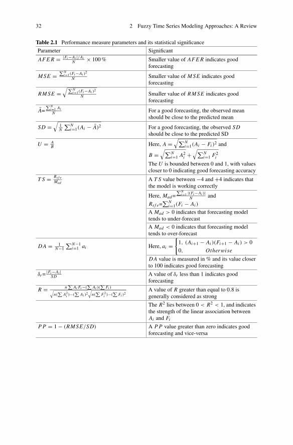
To assess the performance of the time series forecastingmodels (especially FTSmod-els), researchers use numerous performance measure parameters, such as AF E R,M SE , RM SE , A, SD, U , T S, D A, δr , R, R2, P P , etc. All these parameters andtheir statistical significance are presented in Table2.1. In this table, each Fi and Ai isthe forecasted and actual value of day/year i , respectively, and N is the total numberof days/years to be forecasted.

http://dx.doi.org/10.1007/978-3-319-26293-2_6


Table 2.1 Performance measure parameters and its statistical significance

Parameter Significant

AF E R = |Fi −Ai |/AiN × 100% Smaller value of AF E R indicates good

forecasting

M SE =∑N

i=1(Fi −Ai )2

N Smaller value of M SE indicates goodforecasting

RM SE =√∑N

i=1(Fi −Ai )2

N Smaller value of RM SE indicates goodforecasting

A=∑N

i=1 AiN For a good forecasting, the observed mean

should be close to the predicted mean

SD =√

1N

∑Ni=1(Ai − A)2 For a good forecasting, the observed SD

should be close to the predicted SD

U = AB Here, A =

√∑Ni=1(Ai − Fi )2 and

B =√∑N

i=1 A2i +

√∑Ni=1 F2

i

The U is bounded between 0 and 1, with valuescloser to 0 indicating good forecasting accuracy

T S = Rs f eMad

A T S value between −4 and +4 indicates thatthe model is working correctly

Here, Mad=∑N

i=1 |(Fi −Ai )|N and

Rs f e=∑N

i=1(Fi − Ai )

A Mad > 0 indicates that forecasting modeltends to under-forecast

A Mad < 0 indicates that forecasting modeltends to over-forecast

D A = 1N−1

∑N−1i=1 ai Here, ai =

{1, (Ai+1 − Ai )(Fi+1 − Ai ) > 0

0, Otherwise

D A value is measured in % and its value closerto 100 indicates good forecasting

δr=|Fi −Ai |

SD A value of δr less than 1 indicates goodforecasting

R = n∑

Ai Fi −(∑

Ai )(∑

Fi )√n(

∑A2

i )−(∑

Ai )2√

n(∑

F2i )−(

∑Fi )

2A value of R greater than equal to 0.8 isgenerally considered as strong

The R2 lies between 0 < R2 < 1, and indicatesthe strength of the linear association betweenAi and Fi

P P = 1 − (RM SE/SD) A P P value greater than zero indicates goodforecasting and vice-versa

2.7 Conclusion and Discussion 33

2.7 Conclusion and Discussion

From 1994 onwards, numerous time series forecasting models have been proposedbased on the FTS modeling approach.12 Due to the uncertain nature of time series,scope of extensive applications in this domain raised simultaneously with the devel-opment of new algorithms and architectures. The FTSmodeling approach is currentlyapplied to a diverse range of fields from economy, population growth, weather fore-casting, stock index price forecasting to pollution forecasting, etc. Various aspectsof complexities arise in this research domain, if the number of factors in time seriesdata sets is large. These complexities can be evolved in terms of (a) Determinationof length of intervals, (b) Establishment of FLRs between different factors, and (c)Defuzzification of fuzzified time series values.

Present research in the FTS modeling approach mainly aims at designing algo-rithms for discretization of time series data set, rule generation from the fuzzifiedtime series values, proposing techniques for defuzzification operation, and design-ing various hybridized based architectures for resolving complex decision makingproblems.

SC techniques comprise of ANN, RS, EC, and their hybridizations, have recentlybeen employed to solve FTS modeling problems. They endeavor to provide usapproximate results in a very cost effective manner, thereby reducing the time com-plexity. In this survey, a categorization has been presented based on utilization ofdifferent SC techniques with the FTS modeling approach along with basic architec-tures of different hybridized based FTS models.

Fuzzy sets are the oldest component of SC, which is known for representationof real time or uncertain events in a linguistic manner, and can take decisions veryfaster. ANNs are especially used in discovering the rules, and can establish a linearassociation between the inputs and outputs. RSs is mainly employed for extractinghidden patterns from the data in terms of rules. EC provides efficient search algo-rithms to select based intervals from the discretized time series data set, based onsome evaluation criterion.

FTS-ANNhybridization exploits the features of bothANNand fuzzy sets in estab-lishment of FLRs/linguistic rules, data discretization, and defuzzification of fuzzifiedtime series data set. FTS-RS hybridization uses the features of both RS and fuzzysets in discovering meaning full rules from the fuzzified time series data set, therebyemploying these rules in defuzzification operation. FTS-EC hybridization utilizesthe characteristics of both EC and fuzzy sets in the determination of optimal intervallengths of the discretized time series data set, which are further used to represent timeseries data set in terms of fuzzy sets/linguistic terms. From this survey, it is obviousthat the research scope in FTS will be increased in the near future for its flexibility inrepresenting real life problems in a very natural way. This study also describes elab-orately different phases of the FTS modeling approach. Various research issues andchallenges in the FTSmodeling approach are presented in the subsequent section. All

12References are: (Egrioglu et al. 2010, 2011a; Sah and Degtiarev 2005; Wong et al. 2010; Yu2005a).


these inclusions may help the researchers to identify: (a) What are the problems inthe FTS modeling approach?, (b) How to resolve all these problems using heuristicsapproach?, and (c) How to employ different SC methodologies in the FTS modelingapproach to improve its efficiency?

References

Aladag CH, Basaran MA, Egrioglu E, Yolcu U, Uslu VR (2009) Forecasting in high order fuzzytimes series by using neural networks to define fuzzy relations. Expert SystAppl 36(3):4228–4231

Aladag CH, Yolcu U, Egrioglu E (2010) A high order fuzzy time series forecasting model basedon adaptive expectation and artificial neural networks. Math Comput Simul 81(4):875–882

AladagCH,YolcuU,EgriogluE,DalarAZ (2012)Anew time invariant fuzzy time series forecastingmethod based on particle swarm optimization. Appl Soft Comput 12(10):3291–3299

Avazbeigi M, Doulabi SHH, Karimi B (2010) Choosing the appropriate order in fuzzy time series:a new N-factor fuzzy time series for prediction of the auto industry production. Expert Syst Appl37(8):5630–5639

Bahrepour M, Akbarzadeh-T MR, Yaghoobi M, Naghibi-S MB (2011) An adaptive ordered fuzzytime series with application to FOREX. Expert Syst Appl 38(1):475–485

Bai E, Wong WK, Chu WC, Xia M, Pan F (2011) A heuristic time-invariant model for fuzzy timeseries forecasting. Expert Syst Appl 38(3):2701–2707

Bajestani NS, Zare A (2011) Forecasting TAIEX using improved type 2 fuzzy time series. ExpertSyst Appl 38(5):5816–5821

Bang YK, Lee CH (2011) Fuzzy time series prediction using hierarchical clustering algorithms.Expert Syst Appl 38(4):4312–4325

BealeMH, HaganMT, Demuth HB (2010) Neural network Toolbox 7. TheMathWorks Inc, Natick,MA

Bonissone PP (1997) Soft computing: the convergence of emerging reasoning technologies. SoftComput 1:6–18

Brockwell PJ, Davis RA (2008) Introduction to time series and forecasting, 2nd edn. Springer, NewYork

Castro LN, Timmis JI (2003) Artificial immune systems as a novel soft computing paradigm. SoftComput 7:526–544

Chang JR, Lee YT, Liao SY, Cheng CH (2007) Cardinality-based fuzzy time series for forecastingenrollments. New Trends Appl Artif Intell, vol 4570. Springer, Berlin/Heidelberg, pp 735–744

Chatfield C (2000) Time-series forecasting. Chapman and Hall, CRC Press, Boca RatonChen SM (1996) Forecasting enrollments based on fuzzy time series. Fuzzy Sets Syst 81:311–319Chen SM (2002) Forecasting enrollments based on high-order fuzzy time series. Cybern Syst: IntJ 33(1):1–16

Chen SM, Chen CD (2011a) Handling forecasting problems based on high-order fuzzy logicalrelationships. Expert Syst Appl 38(4):3857–3864

Chen SM, Chen CD (2011b) Handling forecasting problems based on high-order fuzzy logicalrelationships. Expert Syst Appl 38(4):3857–3864

Chen SM, Chung NY (2006a) Forecasting enrollments of students by using fuzzy time series andgenetic algorithms. Int J Inf Manag Sci 17(3):1–17

Chen SM, Chung NY (2006b) Forecasting enrollments using high-order fuzzy time series andgenetic algorithms. Int J Intell Syst 21(5):485–501

Chen SM, Hwang JR (2000) Temperature prediction using fuzzy time series. IEEE Trans Syst ManCybern Part B: Cybern 30:263–275

Chen SM, Tanuwijaya K (2011) Multivariate fuzzy forecasting based on fuzzy time series andautomatic clustering techniques. Expert Syst Appl 38(8):10,594–10,605

References 35

Chen SM, Wang NY (2010) Fuzzy forecasting based on fuzzy-trend logical relationship groups.IEEE Trans Syst Man Cybern Part B: Cybern 40(5):1343–1358

ChenTL,ChengCH,TeohHJ (2008)High-order fuzzy time-series based onmulti-period adaptationmodel for forecasting stock markets. Phys A: Stat Mech Appl 387(4):876–888

Chen TY (2012) A signed-distance-based approach to importance assessment and multi-criteriagroup decision analysis based on interval type-2 fuzzy set. Knowl Inf Syst

Chen YS, Cheng CH (2013) Application of rough set classifiers for determining hemodialysisadequacy in ESRD patients. Knowl Inf Syst 34:453–482

Cheng C, Chang J, Yeh C (2006) Entropy-based and trapezoid fuzzification-based fuzzy time seriesapproaches for forecasting IT project cost. Technol Forecast Soc Change 73:524–542

Cheng CH, Cheng GW, Wang JW (2008a) Multi-attribute fuzzy time series method based on fuzzyclustering. Expert Syst Appl 34:1235–1242

Cheng CH,Wang JW, Li CH (2008b) Forecasting the number of outpatient visits using a new fuzzytime series based on weighted-transitional matrix. Expert Syst Appl 34(4):2568–2575

Cheng CH, Chen TL, Wei LY (2010) A hybrid model based on rough sets theory and geneticalgorithms for stock price forecasting. Inf Sci 180(9):1610–1629

Cheng CH, Huang SF, Teoh HJ (2011) Predicting daily ozone concentration maxima using fuzzytime series based on a two-stage linguistic partitionmethod. ComputMathAppl 62(4):2016–2028

Cheng CH, Wei LY, Liu JW, Chen TL (2013) OWA-based ANFIS model for TAIEX forecasting.Econ Modell 30:442–448

Czibula G, Czibula IG, Gaceanu RD (2013) Intelligent data structures selection using neural net-works. Knowl Inf Syst 34:171–192

Donaldson RG, Kamstra M (1996) Forecast combining with neural networks. J Forecast 15(1):49–61

DoteY,OvaskaSJ (2001) Industrial applications of soft computing: a review.Proc IEEE89(9):1243–1265

Eberhart R, Kennedy J (1995) A new optimizer using particle swarm theory. In: Proceedings of thesixth international symposium on micro machine and human science, Nagoya, pp 39–43

Eberhart R, Shi Y (2001) Particle swarm optimization: Developments, applications and resources.In: Proceedings of the IEEE international conference on evolutionary computation, Brisbane,Australia, pp 591–600

Egrioglu E, Aladag CH, Yolcu U, Basaran MA, Uslu VR (2009) A new hybrid approach based onSARIMA and partial high order bivariate fuzzy time series forecasting model. Expert Syst Appl36(4):7424–7434

Egrioglu E, Aladag CH, Yolcu U, Uslu VR, Basaran MA (2010) Finding an optimal interval lengthin high order fuzzy time series. Expert Syst Appl 37(7):5052–5055

Egrioglu E, Aladag CH, Basaran MA, Yolcu U, Uslu VR (2011a) A new approach based on theoptimization of the length of intervals in fuzzy time series. J Intell Fuzzy Syst 22(1):15–19

Egrioglu E, Aladag CH, Yolcu U, Uslu V, Erilli N (2011b) Fuzzy time series forecasting methodbased on Gustafson-Kessel fuzzy clustering. Expert Syst Appl 38(8):10355–10357

Estivill-Castro V (2002) Why so many clustering algorithms: a position paper. ACM SIGKDDExplor Newslett 4(1):65–75

Gangwar SS, Kumar S (2012) Partitions based computational method for high-order fuzzy timeseries forecasting. Expert Systems with Applications 39(15):12,158–12,164

Gaume E, Gosset R (2003) Over-parameterisation, a major obstacle to the use of artificial neuralnetworks in hydrology? Hydrol Earth Syst Sci 7(5):693–706

Gen M, Cheng R (1997) Genetic algorithms and engineering design. Wiley, New YorkGoldberg DE (1989) Genetic algorithm in search, optimization, and machine learning. Addison-Wesley, Massachusetts

Gondek D, Hofmann T (2007) Non-redundant data clustering. Knowl Inf Syst 12:1–24Greenfield S, Chiclana F (2013) Accuracy and complexity evaluation of defuzzification strategiesfor the discretised interval type-2 fuzzy set. Int J Approximate Reasoning 54(8):1013–1033


Haykin S (1999) Neural Networks, a comprehensive foundation. Macmillan College PublishingCo., New York

Herrera-Viedma E, Cabrerizo FJ, Kacprzyk J, PedryczW (2014) A review of soft consensus modelsin a fuzzy environment. Information Fusion 17:4–13

Holland JH (1975) Adaptation in natural and artificial systems. MIT Press, CambridgeHornik K, StinchcombeM,White H (1989) Multilayer feedforward networks are universal approx-imators. Neural Netw 2(5):359–366

Hsu YY, Tse SM, Wu B (2003) A new approach of bivariate fuzzy time series analysis to theforecasting of a stock index. Int J Uncertain Fuzziness Knowl-Based Syst 11(6):671–690

HuangYL,Horng SJ,HeM, Fan P,KaoTW,KhanMK,Lai JL,Kuo IH (2011a)A hybrid forecastingmodel for enrollments based on aggregated fuzzy time series and particle swarm optimization.Expert Syst Appl 38(7):8014–8023

Huang YL, Horng SJ, Kao TW, Run RS, Lai JL, Chen RJ, Kuo IH, KhanMK (2011b) An improvedforecasting model based on the weighted fuzzy relationship matrix combined with a PSO adap-tation for enrollments. Int J Innov Comput Inf Control 7(7A):4027–4046

HuarngK (2001)Heuristicmodels of fuzzy time series for forecasting. FuzzySets Systems123:369–386

Huarng K, Yu HK (2005) A Type 2 fuzzy time series model for stock index forecasting. Phys A:Stat Mech Appl 353:445–462

Huarng K, Yu THK (2006a) The application of neural networks to forecast fuzzy time series. PhysA: Stat Mech Appl 363(2):481–491

Huarng K, Yu THK (2006b) Ratio-based lengths of intervals to improve fuzzy time series forecast-ing. IEEE Trans Syst Man Cybern Part B: Cybern 36(2):328–340

Huarng KH, Yu THK (2012) Modeling fuzzy time series with multiple observations. Int J InnovComput Inf Control 8(10(B)):7415–7426

Huarng KH, Yu THK, Hsu YW (2007) A multivariate heuristic model for fuzzy time-series fore-casting. IEEE Trans Syst Man Cybern Part B: Cybern 37:836–846

Hwang JR, Chen SM, Lee CH (1998) Handling forecasting problems using fuzzy time series. FuzzySets Syst 100:217–228

Indro DC et al (1999) Predicting mutual fund performance using artificial neural networks. Omega27(3):373–380

Jang JSR, Sun CT, Mizutani E (1997) Neuro-fuzzy and soft computing: a computational approachto learning and machine intelligence. Prentice-Hall, London

Jiang Y, Li X, Huang C, Wu X (2013) Application of particle swarm optimization based on CHKSsmoothing function for solving nonlinear bilevel programming problem. Appl Math Comput219(9):4332–4339

Jilani TA, Burney SMA (2008) A refined fuzzy time series model for stock market forecasting.Phys A 387(12):2857–2862

Kacprzyk J (2010) Advances in soft computing, vol 7095. Springer, HeidelbergKennedy J, Eberhart R (1995) Particle swarm optimization. In: IEEE international conference onneural networks, Perth, WA 4:1942–1948

Keogh E, Lin J (2005) Clustering of time-series subsequences is meaningless: implications forprevious and future research. Knowl Inf Syst 8(2):154–177

Kohonen T (1990) The self organizing maps. In: Proceedings of the IEEE, vol 78, pp 1464–1480KuligowskiRJ,BarrosAP (1998)Experiments in short-termprecipitation forecasting using artificialneural networks. Mon Weather Rev 126:470–482

Kumar K, Bhattacharya S (2006) Artificial neural network vs. linear discriminant analysis in creditratings forecast: A comparative study of prediction performances. Review of Accounting andFinance 5(3):216–227

Kumar S (2004) Neural networks: a classroom approach. Tata McGraw-Hill Education Pvt. Ltd.,New Delhi

References 37

Kuo IH, Horng SJ, Kao TW, Lin TL, Lee CL, Pan Y (2009) An improved method for forecastingenrollments based on fuzzy time series and particle swarm optimization. Expert Syst Appl 36(3,Part 2):6108–6117

Kuo IH,HorngSJ,ChenYH,RunRS,KaoTW,ChenRJ, Lai JL, LinTL (2010) ForecastingTAIFEXbased on fuzzy time series and particle swarm optimization. Expert Syst Appl 37(2):1494–1502

Law R (2000) Back-propagation learning in improving the accuracy of neural network-basedtourism demand forecasting. Tour Manag 21(4):331–340

Lee HS, Chou MT (2004) Fuzzy forecasting based on fuzzy time series. Int J Comput Math81(7):781–789

Lee LW,Wang LH, Chen SM, Leu YH (2006) Handling forecasting problems based on two-factorshigh-order fuzzy time series. IEEE Trans Fuzzy Syst 14:468–477

Lee LW, Wang LH, Chen SM (2007) Temperature prediction and TAIFEX forecasting based onfuzzy logical relationships and genetic algorithms. Expert Syst Appl 33(3):539–550

Lee LW, Wang LH, Chen SM (2008) Temperature prediction and TAIFEX forecasting based onhigh-order fuzzy logical relationships and genetic simulated annealing techniques. Expert SystAppl 34(1):328–336

Lee ZY (2006) Method of bilaterally bounded to solution blasius equation using particle swarmoptimization. Appl Math Comput 179(2):779–786

Lertworaprachaya Y, Yang Y, John R (2010) High-order Type-2 fuzzy time series. Internationalconference of soft computing and pattern recognition. IEEE, Paris, pp 363–368

Li ST, ChengYC (2007) Deterministic fuzzy time seriesmodel for forecasting enrollments. ComputMath Appl 53(12):1904–1920

Li ST, Cheng YC, Lin SY (2008) A FCM-based deterministic forecasting model for fuzzy timeseries. Comput Math Appl 56(12):3052–3063

Li ST, Kuo SC, Cheng YC, Chen CC (2011) A vector forecasting model for fuzzy time series. ApplSoft Comput 11(3):3125–3134

Li ST et al (2010) Deterministic vector long-term forecasting for fuzzy time series. Fuzzy Sets Syst161(13):1852–1870

Liao TW (2005) Clustering of time series data - a survey. Pattern Recogn 38(11):1857–1874Lin SY, Horng SJ, Kao TW, Huang DK, Fahn CS, Lai JL, Chen RJ, Kuo IH (2010a) An efficient bi-objective personnel assignment algorithm based on a hybrid particle swarm optimization model.Expert Syst Appl 37(12):7825–7830

Lin TL, Horng SJ, Kao TW, Chen YH, Run RS, Chen RJ, Lai JL, Kuo IH (2010b) An efficient job-shop scheduling algorithm based on particle swarm optimization. Expert Syst Appl 37(3):2629–2636

Liu HT (2007) An improved fuzzy time series forecasting method using trapezoidal fuzzy numbers.Fuzzy Optim Decis Making 6:63–80

Liu HT, Wei ML (2010) An improved fuzzy forecasting method for seasonal time series. ExpertSyst Appl 37(9):6310–6318

Liu HT, Wei NC, Yang CG (2009) Improved time-variant fuzzy time series forecast. Fuzzy OptimDecis Making 8:45–65

Liu Y, Starzyk JA, Zhu Z (2008) Optimized approximation algorithm in neural networks withoutoverfitting. IEEE Trans Neural Netw 19(6):983–995

Mencattini A, Salmeri M, Bertazzoni S, Lojacono R, Pasero E, Moniaci W (2005) Local meteoro-logical forecasting by type-2 fuzzy systems time series prediction. IEEE International conferenceon computational intelligence for measurement systems and applications. Giardini Naxos, Italy,pp 20–22

Mitra S, Pal SK, Mitra P (2002) Data mining in soft computing framework: a survey. IEEE TransNeural Netw 13(1):3–14

Montalvo I, Izquierdo J, Pérez R, Tung MM (2008) Particle swarm optimization applied to thedesign of water supply systems. Comput Math Appl 56(3):769–776


Ordonez C (2003) Clustering binary data streams with K-means. In: Proceedings of the 8th ACMSIGMOD workshop on Research issues in data mining and knowledge discovery. ACM Press,New York, USA, pp 12–19

Own CM, Yu PT (2005) Forecasting fuzzy time series on a heuristic high-order model. CybernSyst: Int J 36(7):705–717

Pattaraintakorn P, Cercone N (2008) Integrating rough set theory and medical applications. ApplMath Lett 21(4):400–403

Pawlak Z (1982) Rough sets. Int J Comput Inf Sci 11(5):341–356Pawlak Z (1991) Rough sets: theoretical aspects of reasoning about data. Kluwer Academic Pub-lishers

Pedrycz W, Sosnowski Z (2005) C-Fuzzy decision trees. IEEE Trans Syst Man Cybern C Appl Rev35(4):498–511

Piotrowski AP, Napiorkowski JJ (2012) A comparison of methods to avoid overfitting in neuralnetworks training in the case of catchment runoff modelling. J Hydrol

QiuW, Liu X, Li H (2011) A generalized method for forecasting based on fuzzy time series. ExpertSyst Appl 38(8):10446–10453

Qiu W, Liu X, Wang L (2012) Forecasting shanghai composite index based on fuzzy time seriesand improved C-fuzzy decision trees. Expert Syst Appl 39(9):7680–7689

Ross TJ (2007) Fuzzy Logic with engineering applications. John Wiley and Sons, SingaporeSah M, Degtiarev K (2005) Forecasting enrollment model based on first-order fuzzy time series.Prec World Acad Sci Eng Technol 1:132–135

Singh P, Borah B (2012) An effective neural network and fuzzy time series-based hybridized modelto handle forecasting problems of two factors. Knowl Inf Syst 38(3):669–690

Singh P, Borah B (2013a) Forecasting stock index price based on M-factors fuzzy time series andparticle swarm optimization. International Journal of Approximate Reasoning

Singh P, Borah B (2013b) High-order fuzzy-neuro expert system for daily temperature forecasting.Knowl-Based Syst 46:12–21

Singh SR (2007a) A robust method of forecasting based on fuzzy time series. Appl Math Comput188(1):472–484

Singh SR (2007b) A simple method of forecasting based on fuzzy time series. Appl Math Comput186(1):330–339

Singh SR (2007c) A simple time variant method for fuzzy time series forecasting. Cybernetics andSystems: An International Journal 38(3):305–321

Singh SR (2008) A computational method of forecasting based on fuzzy time series. Math ComputSimul 79(3):539–554

Singh SR (2009) A computational method of forecasting based on high-order fuzzy time series.Expert Syst Appl 36(7):10,551–10,559

Sivanandam SN, Deepa SN (2007) Principles of soft computing. Wiley India (P) Ltd., New DelhiSong Q, Chissom BS (1993a) Forecasting enrollments with fuzzy time series - Part I. Fuzzy SetsSyst 54(1):1–9

Song Q, Chissom BS (1993b) Fuzzy time series and its models. Fuzzy Sets Syst 54(1):1–9Song Q, Chissom BS (1994) Forecasting enrollments with fuzzy time series - Part II. Fuzzy SetsSyst 62(1):1–8

Szmidt E, Kacprzyk J, Bujnowski P (2014) How to measure the amount of knowledge conveyedby atanassov’s intuitionistic fuzzy sets. Inf Sci 257:276–285

Tan PN, Steinbach M, Kumar V (2009) Introduction to data mining, 4th edn. Dorling KindersleyPublishing Inc, India

Taylor JW, Buizza R (2002) Neural network load forecasting with weather ensemble predictions.IEEE Trans Power Syst 17:626–632

Teoh HJ, Cheng CH, Chu HH, Chen JS (2008) Fuzzy time series model based on probabilisticapproach and rough set rule induction for empirical research in stock markets. Data Knowl Eng67(1):103–117

References 39

TeohHJ,ChenTL,ChengCH,ChuHH (2009)Ahybridmulti-order fuzzy time series for forecastingstock markets. Expert Syst Appl 36(4):7888–7897

Trelea IC (2003) The particle swarm optimization algorithm: convergence analysis and parameterselection. Inf Process Lett 85(6):317–325

Tsai CC,Wu SJ (2000) Forecasting enrolments with high-order fuzzy time series. 19th Internationalconference of the North American. Fuzzy Information Processing Society, Atlanta, GA, pp 196–200

Tsaur RC, Yang JCO, Wang HF (2005) Fuzzy relation analysis in fuzzy time series model. ComputMath Appl 49(4):539–548

Venkatesan C, Raskar SD, Tambe SS, Kulkarni BD, Keshavamurty RN (1997) Prediction of allIndia summer monsoon rainfall using error-back-propagation neural networks. Meteorol AtmosPhys 62:225–240

Wan Z, Wang G, Sun B (2013) A hybrid intelligent algorithm by combining particle swarm opti-mization with chaos searching technique for solving nonlinear bilevel programming problems.Swarm Evol Comput 8:26–32

Wei LY, Chen TL, Ho TH (2011) A hybrid model based on adaptive-network-based fuzzy inferencesystem to forecast Taiwan stock market. Expert Syst Appl 38(11):13,625–13,631

Weigend A (1994) An overfitting and the effective number of hidden units. In: Mozer MC, Smolen-sky P, Weigend AS (eds) Proceedings of the 1993 Connectionist Models Summer School.Lawrence Erlbaum Associates, Hillsdale, NJ, pp 335–342

Wilson ID, Paris SD,Ware JA, Jenkins DH (2002) Residential property price time series forecastingwith neural networks. Knowl-Based Syst 15(5–6):335–341

WongWK,Bai E,ChuAWC(2010)Adaptive time-variantmodels for fuzzy-time-series forecasting.IEEE Trans Syst Man Cybern Part B: Cybern 40:453–482

Wu X et al (2008) Top 10 algorithms in data mining. Knowl Inf Syst 14:1–37Xiong Y, Yeung DY (2002) Mixtures of ARMA models for model-based time series clustering. In:IEEE International conference on data mining, Los Alamitos, USA, pp 717–720

Yardimci A (2009) Soft computing in medicine. Appl Soft Comput 9(3):1029–1043Yolcu U et al (2011) Time-series forecasting with a novel fuzzy time-series approach: an examplefor Istanbul stock market. Journal of Statistical Computation and Simulation

Yu HK (2005a) A refined fuzzy time-series model for forecasting. Phys A 346(3–4):657–681Yu HK (2005b) Weighted fuzzy time series models for TAIEX forecasting. Phys A 349(3–4):609–624

YuTHK,HuarngKH(2010)Aneural network-based fuzzy time seriesmodel to improve forecasting.Expert Syst Appl 37(4):3366–3372

Zadeh LA (1965) Fuzzy sets. Inf Control 8(3):338–353Zadeh LA (1971) Similarity relations and fuzzy orderings. Inf Sci 3:177–200Zadeh LA (1973) Outline of a new approach to the analysis of complex systems and decisionprocesses. IEEE Trans Syst Man Cybern SMC-3:28–44

Zadeh LA (1975a) The concept of a linguistic variable and its application to approximate reasoning- I. Inf Sci 8(3):199–249

Zadeh LA (1975b) The concept of a linguistic variable and its application to approximate reasoning-III. Inf Sci 9(1):43–80

Zadeh LA (1989) Knowledge representation in fuzzy logic. IEEE Trans Knowl Data Eng 1(1):89–100

Zadeh LA (1994) Fuzzy logic, neural networks, and soft computing. Commun ACM 37(3):77–84Zadeh LA (1997) The roles of fuzzy logic and soft computing in the conception, design and deploy-ment of intelligent systems. In: Software agents and soft computing, pp 183–190

Zadeh LA (2002) From computing with numbers to computing with words - From manipulation ofmeasurements to manipulation of perceptions. Int J Appl Math Comput Sci 12(3):307–324

http://www.springer.com/978-3-319-26292-5

Documents

Fuzzy Time Series Modeling Approaches: A Review