Embed Size (px)
DESCRIPTION
FW364 Ecological Problem Solving. Class 21: Predation. November 18, 2013. Outline for Today. Continuing with our shift in focus from populations of single species to community interactions Objectives from Last Classes: Expanded predator-prey models - PowerPoint PPT Presentation
Citation preview
FW364 Ecological Problem Solving
Class 21: Predation
November 18, 2013
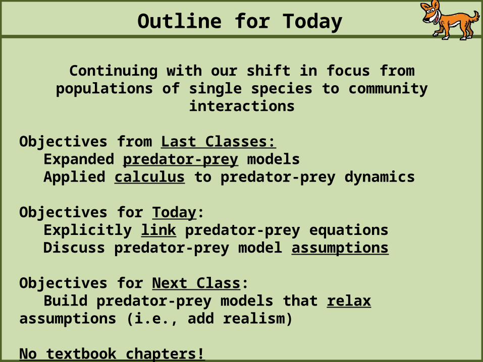
Continuing with our shift in focus frompopulations of single species to community interactions
Objectives from Last Classes:Expanded predator-prey modelsApplied calculus to predator-prey dynamics
Objectives for Today:Explicitly link predator-prey equationsDiscuss predator-prey model assumptions
Objectives for Next Class:Build predator-prey models that relax assumptions (i.e., add realism)
No textbook chapters!
Outline for Today
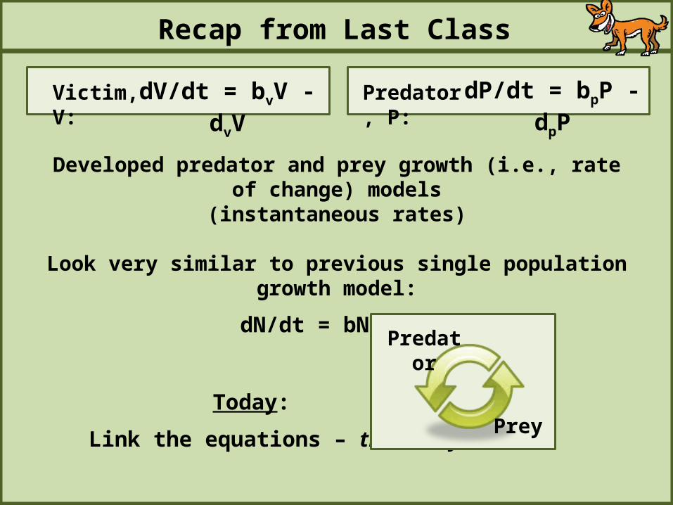
Recap from Last Class
Victim, V: Predator, P:dV/dt = bvV - dvV dP/dt = bpP - dpP
Developed predator and prey growth (i.e., rate of change) models(instantaneous rates)
Look very similar to previous single population growth model:
dN/dt = bN – dN
Today:
Link the equations – this is key!
Predator
Prey
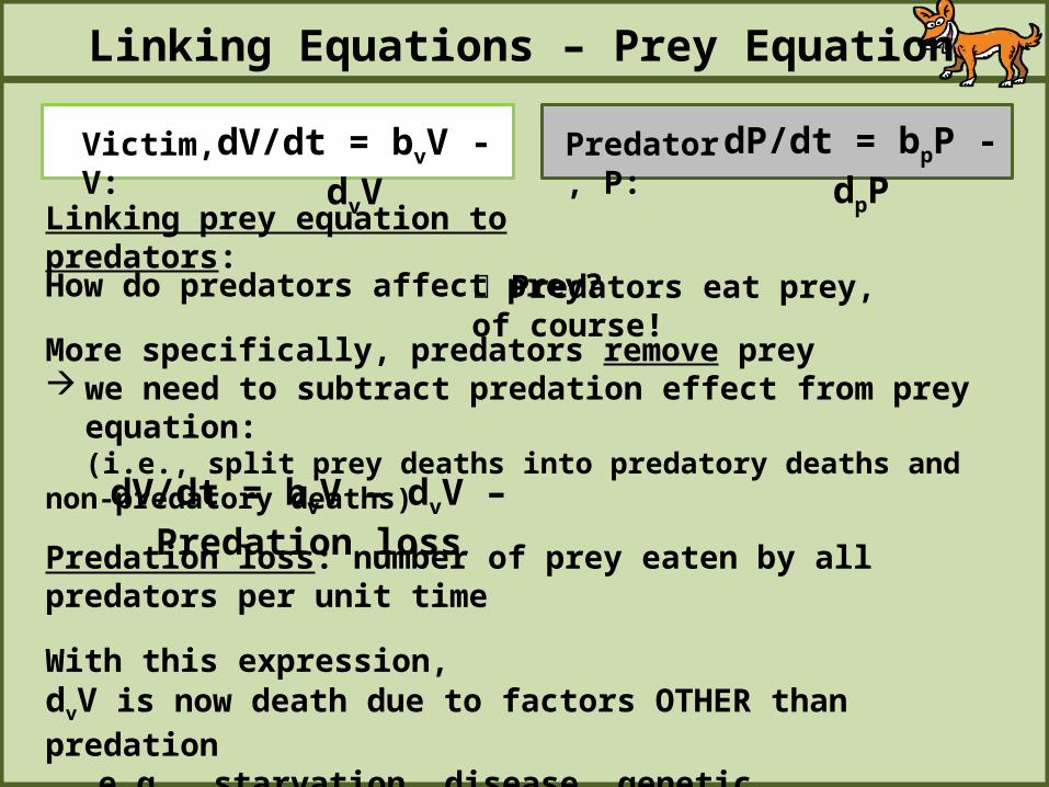
Linking Equations – Prey Equation
Victim, V: Predator, P:dV/dt = bvV - dvV dP/dt = bpP - dpP
Linking prey equation to predators:
How do predators affect prey?
More specifically, predators remove prey we need to subtract predation effect from prey equation:
(i.e., split prey deaths into predatory deaths and non-predatory deaths)
dV/dt = bvV – dvV – Predation loss
Predation loss: number of prey eaten by all predators per unit time
With this expression,dvV is now death due to factors OTHER than predation
e.g., starvation, disease, genetic effects, etc.
Predators eat prey, of course!
Victim, V: Predator, P:dV/dt = bvV - dvV dP/dt = bpP - dpP
dV/dt = bvV – dvV – Predation loss
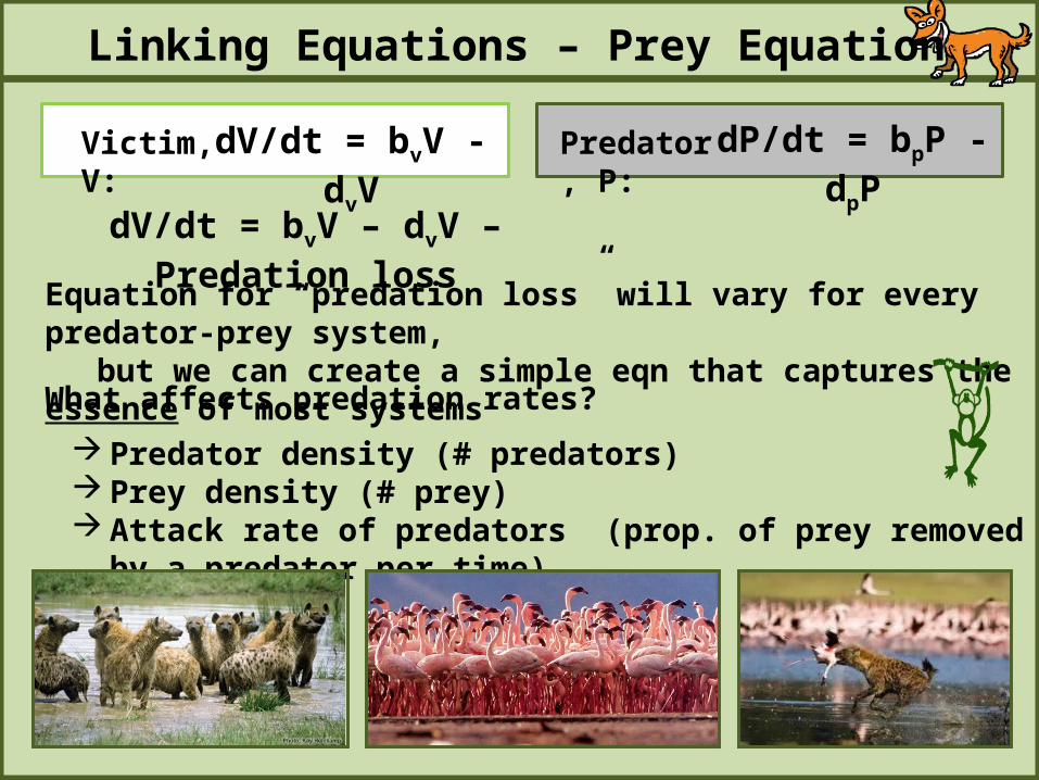
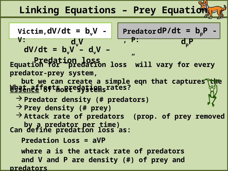
Equation for “predation loss” will vary for every predator-prey system,but we can create a simple eqn that captures the essence of most systems
What affects predation rates?
Predator density (# predators) Prey density (# prey) Attack rate of predators (prop. of prey removed by a predator per time)
Linking Equations – Prey Equation
Victim, V: Predator, P:dV/dt = bvV - dvV dP/dt = bpP - dpP
dV/dt = bvV – dvV – Predation loss
Equation for “predation loss” will vary for every predator-prey system,but we can create a simple eqn that captures the essence of most systems
What affects predation rates?
Predator density (# predators) Prey density (# prey) Attack rate of predators (prop. of prey removed by a predator per time)
Can define predation loss as:
Predation Loss = aVPwhere a is the attack rate of predatorsand V and P are density (#) of prey and predators
Linking Equations – Prey Equation
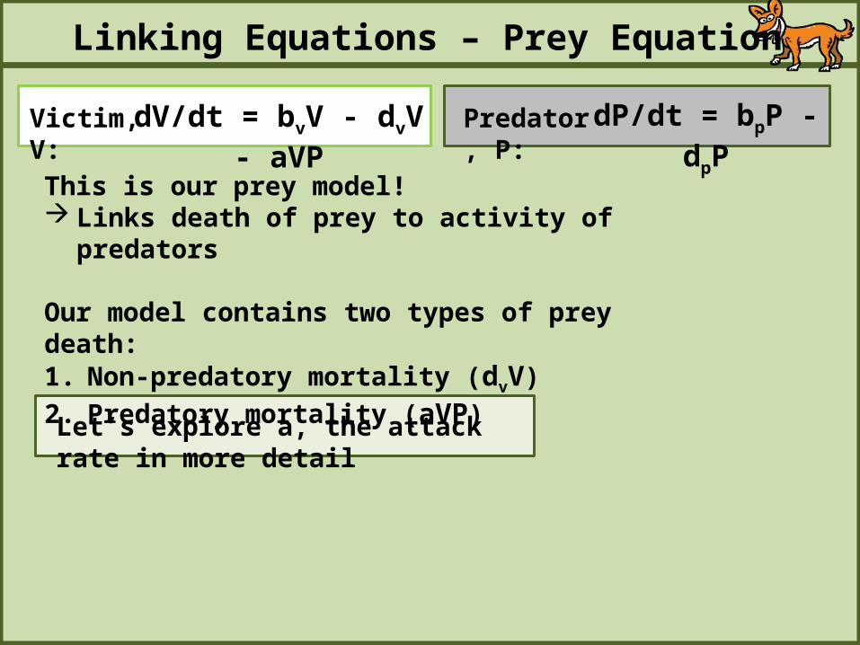
Victim, V: Predator, P:dV/dt = bvV - dvV - aVP dP/dt = bpP - dpP
This is our prey model! Links death of prey to activity of predators
Our model contains two types of prey death:1. Non-predatory mortality (dvV)
2. Predatory mortality (aVP)
Let’s explore a, the attack rate in more detail
Linking Equations – Prey Equation
Victim, V: Predator, P:dV/dt = bvV - dvV - aVP dP/dt = bpP - dpP
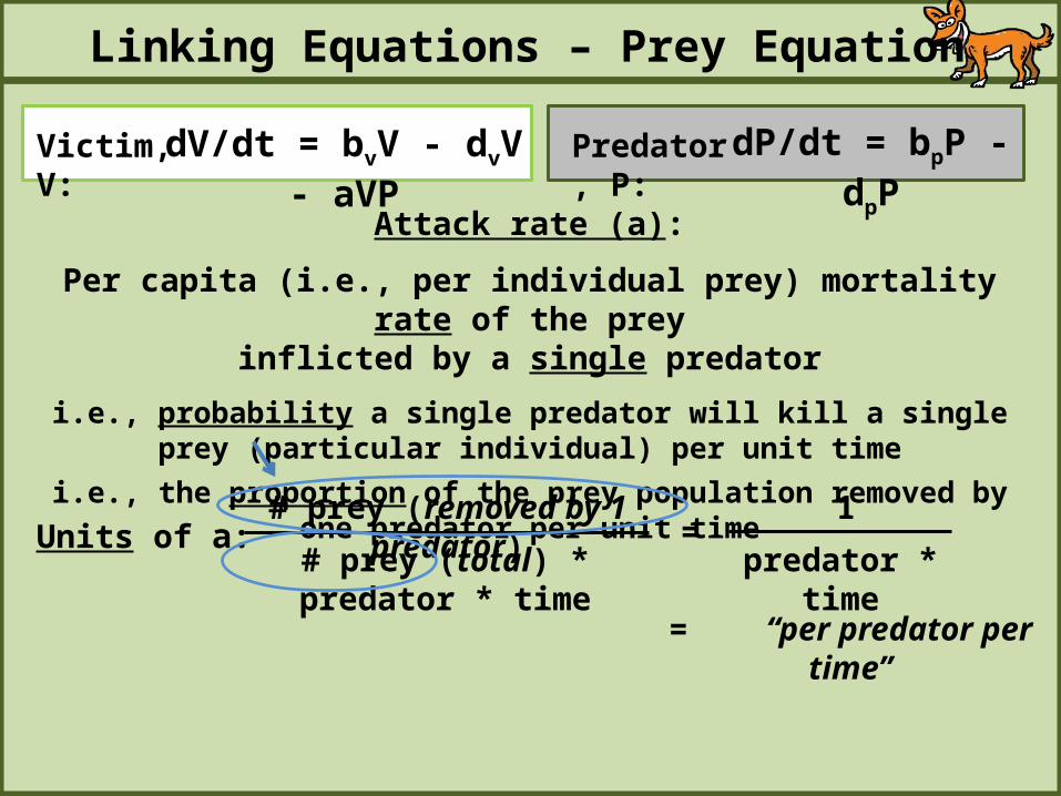
Attack rate (a):
Per capita (i.e., per individual prey) mortality rate of the preyinflicted by a single predator
i.e., probability a single predator will kill a single prey (particular individual) per unit time
i.e., the proportion of the prey population removed by one predator per unit time
1
predator * time=
# prey (removed by 1 predator)
# prey (total) * predator * timeUnits of a:
= “per predator per time”
Linking Equations – Prey Equation

Victim, V: Predator, P:dV/dt = bvV - dvV - aVP dP/dt = bpP - dpP
Attack rate (a):
Per capita (i.e., per individual prey) mortality rate of the preyinflicted by a single predator
i.e., probability a single predator will kill a single prey (particular individual) per unit time
i.e., the proportion of the prey population removed by one predator per unit time
Linking Equations – Prey Equation
Example - How a proportion can also be a per capita mortality:
There are 200 prey. A single predator can attack 20 prey in one time step.
The proportion of prey population attacked by one predator = 20/200 = 0.10
Which means a single prey has a 10% chance of being attacked by one predator i.e., per capita mortality rate of 0.10 a = 0.10 /(pred*time)
Victim, V: Predator, P:dV/dt = bvV - dvV - aVP dP/dt = bpP - dpP
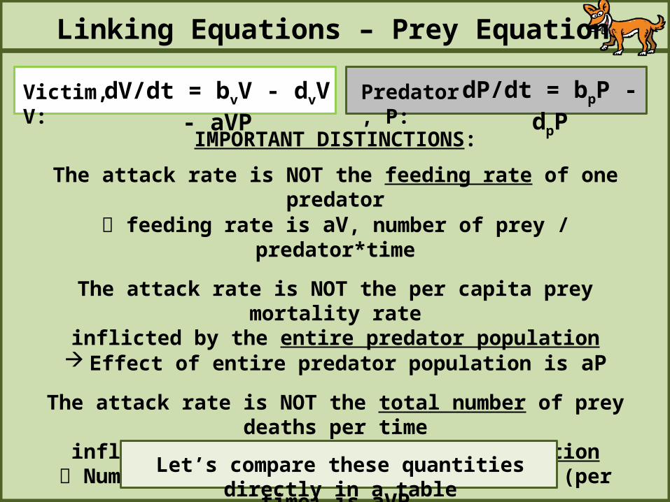
IMPORTANT DISTINCTIONS:
The attack rate is NOT the feeding rate of one predator feeding rate is aV, number of prey / predator*time
The attack rate is NOT the per capita prey mortality rateinflicted by the entire predator population
Effect of entire predator population is aP
The attack rate is NOT the total number of prey deaths per timeinflicted by the entire predator population
Number of prey deaths due to predation (per time) is aVP
These are important (and conceptually challenging) distinctions!
Let’s compare these quantities directly in a table
Linking Equations – Prey Equation
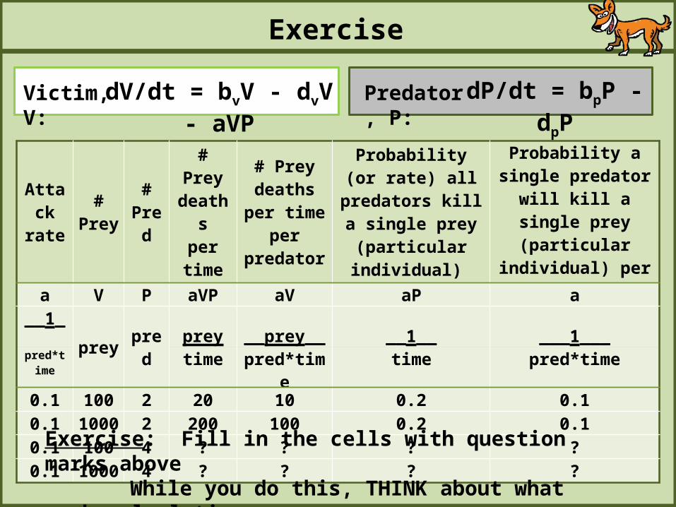
Victim, V: Predator, P:dV/dt = bvV - dvV - aVP dP/dt = bpP - dpP
Attack rate
#Prey
#Pred
# Prey deaths
per time
# Prey deaths
per timeper predator
Probability (or rate) all predators kill a single
prey(particular individual)
Probability a single predator will kill a
single prey (particular individual) per unit time
a V P aVP aV aP a
__1__ prey pred prey __prey__ __1__ ___1___pred*time time pred*time time pred*time
0.1 100 2 20 10 0.2 0.10.1 1000 2 200 100 0.2 0.10.1 100 4 ? ? ? ?0.1 1000 4 ? ? ? ?
Exercise: Fill in the cells with question marks aboveWhile you do this, THINK about what each calculation means
Exercise
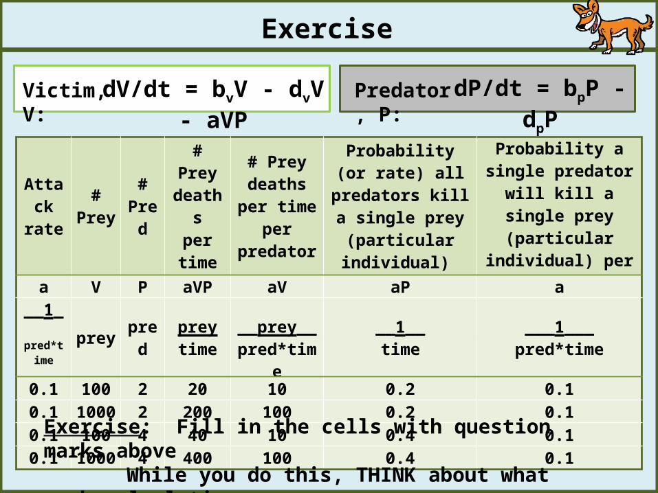
Exercise
Victim, V: Predator, P:dV/dt = bvV - dvV - aVP dP/dt = bpP - dpP
Attack rate
#Prey
#Pred
# Prey deaths
per time
# Prey deaths
per timeper predator
Probability (or rate) all predators kill a single
prey(particular individual)
Probability a single predator will kill a
single prey (particular individual) per unit time
a V P aVP aV aP a
__1__ prey pred prey __prey__ __1__ ___1___pred*time time pred*time time pred*time
0.1 100 2 20 10 0.2 0.10.1 1000 2 200 100 0.2 0.10.1 100 4 40 10 0.4 0.10.1 1000 4 400 100 0.4 0.1
Exercise: Fill in the cells with question marks aboveWhile you do this, THINK about what each calculation means
Linking Equations
Victim, V: Predator, P:dV/dt = bvV - dvV - aVP dP/dt = bpP - dpP
That’s it for the prey model!
Let’s move on to the predator model
Victim, V: Predator, P:dV/dt = bvV - dvV - aVP dP/dt = bpP - dpP
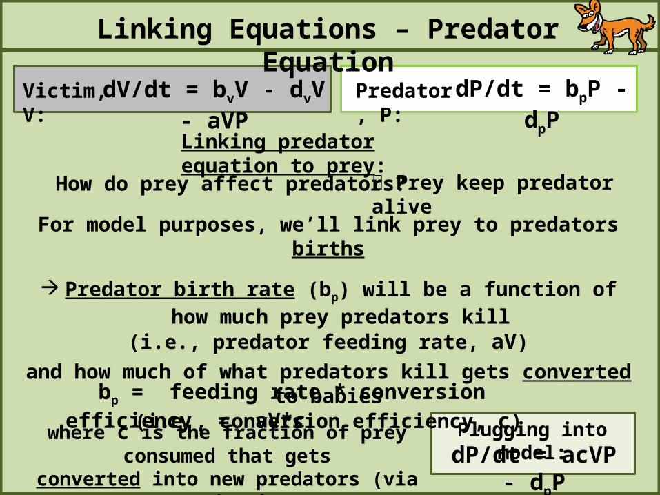
Linking predator equation to prey:
How do prey affect predators?
For model purposes, we’ll link prey to predators births
Predator birth rate (bp) will be a function of how much prey predators kill(i.e., predator feeding rate, aV)
and how much of what predators kill gets converted to babies(i.e., conversion efficiency, c)
Prey keep predator alive
bp = feeding rate * conversion efficiency = aV*c
where c is the fraction of prey consumed that getsconverted into new predators (via reproduction) dP/dt = acVP - dpP
Plugging into model:
Linking Equations – Predator Equation
Linking Equations
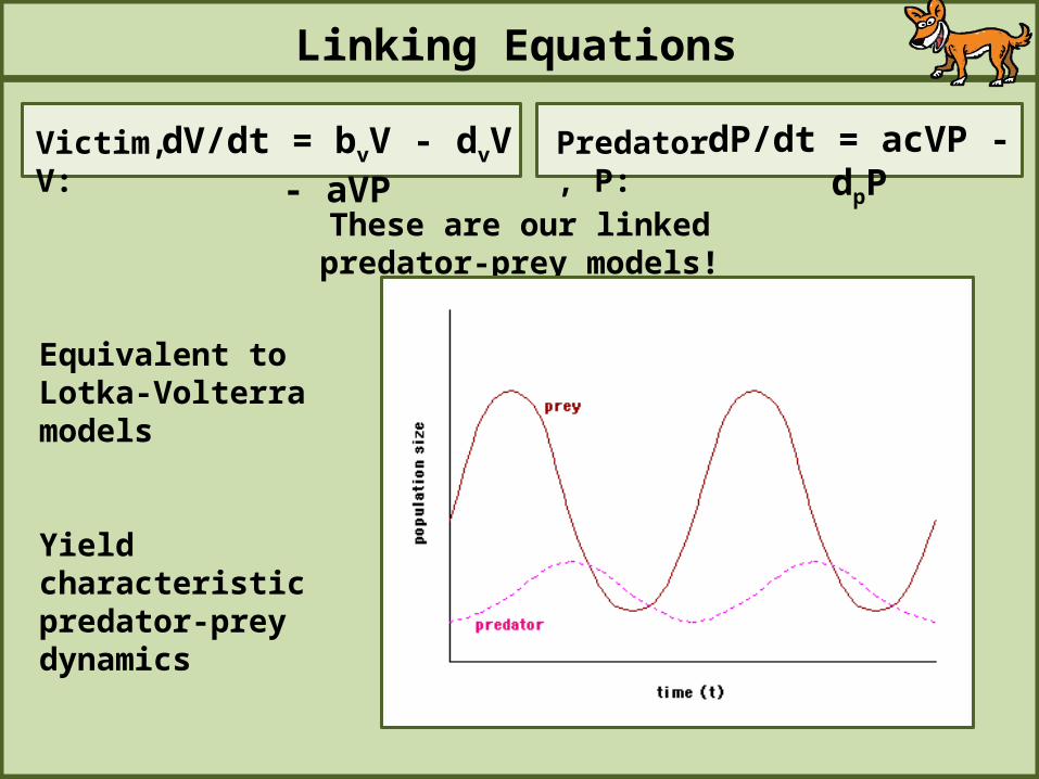
Victim, V: Predator, P:dV/dt = bvV - dvV - aVP dP/dt = acVP - dpP
These are our linked predator-prey models!
Equivalent toLotka-Volterra models
Yield characteristicpredator-prey dynamics
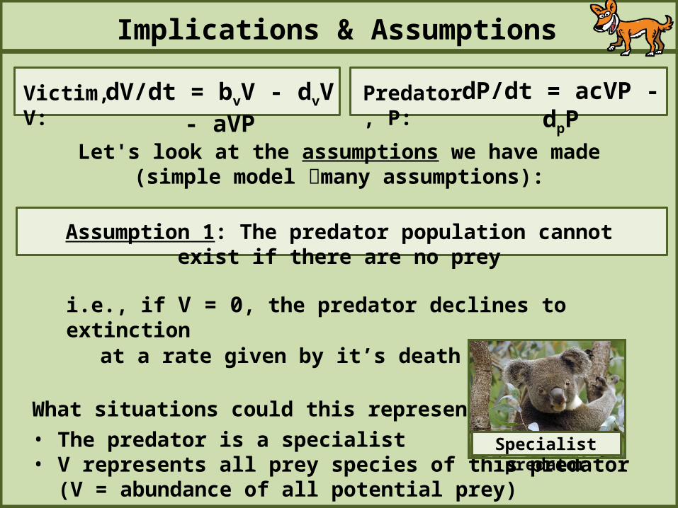
Let's look at the assumptions we have made(simple model many assumptions):
Assumption 1: The predator population cannot exist if there are no prey
i.e., if V = 0, the predator declines to extinctionat a rate given by it’s death rate (dp)
What situations could this represent?
• The predator is a specialist• V represents all prey species of this predator
(V = abundance of all potential prey)
Implications & Assumptions
Victim, V: Predator, P:dV/dt = bvV - dvV - aVP dP/dt = acVP - dpP
Specialist predator
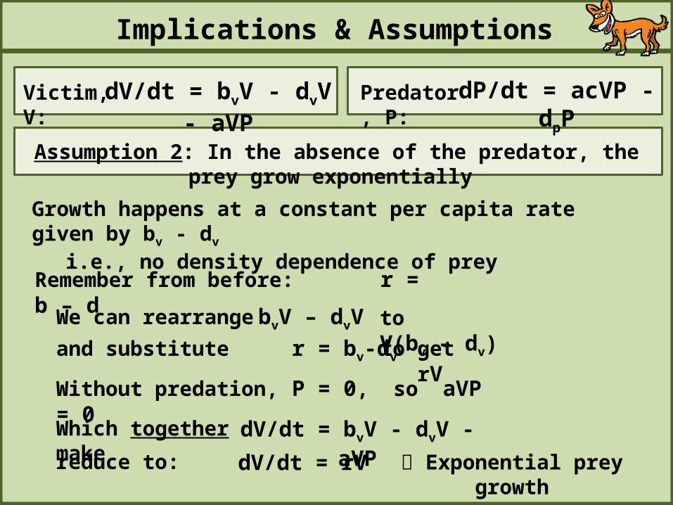
Assumption 2: In the absence of the predator, the prey grow exponentially
Implications & Assumptions
Victim, V: Predator, P:dV/dt = bvV - dvV - aVP dP/dt = acVP - dpP
We can rearrange bvV – dvV
dV/dt = bvV - dvV - aVP
Growth happens at a constant per capita rate given by bv - dv
i.e., no density dependence of prey
Remember from before: r = b – d
to V(bv – dv)and substitute r = bv-dv
Without predation, P = 0, so aVP = 0
Which together make
dV/dt = rVreduce to:
to get rV
Exponential prey growth
Assumption 3: Predators encounter prey randomly (“well-mixed” environment)
Implications & Assumptions
Victim, V: Predator, P:dV/dt = bvV - dvV - aVP dP/dt = acVP - dpP
Mathematically, we represent the random encounter by multiplying V and P(as done in the aVP term for prey and acVP for predators)
Random encounter is based on the rule for probability of independent events
We assume the distributions of predators and prey are independent of each other
i.e., prey do not have a refuge from predation (no spatial structure)predators do not aggregate to areas with higher prey
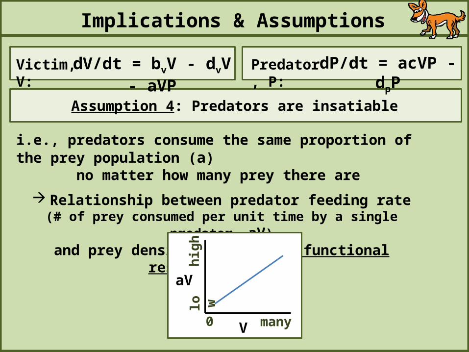
Assumption 4: Predators are insatiable
Implications & Assumptions
Victim, V: Predator, P:dV/dt = bvV - dvV - aVP dP/dt = acVP - dpP
i.e., predators consume the same proportion of the prey population (a) no matter how many prey there are
Relationship between predator feeding rate(# of prey consumed per unit time by a single predator, aV)
and prey density is a linear functional response (Type I)
V
aV
low
0 many
high
Assumption 5: No age / stage structure
Implications & Assumptions
Victim, V: Predator, P:dV/dt = bvV - dvV - aVP dP/dt = acVP - dpP
Assumption 6: Predators do not interact with each other…
… other than by consuming the same resource i.e., no aggression, no territoriality
What type of density dependence do these predators have? scramble predators
That’s it for the assumptions!
Next class we will relax three of these assumptions
Predator-Prey Dynamics
Victim, V: Predator, P:dV/dt = bvV - dvV - aVP dP/dt = acVP - dpP
Equations express rate of change in predators and prey…… not abundance of predators and prey at particular times
An important aspect of these equations:
To compare to previous equations,Our predator-prey equations are like: dN/dt = bN – dN
NOT Nt = N0ert
Remember how we derived Nt = N0ert
from dN/dt = bN – dN ? ….
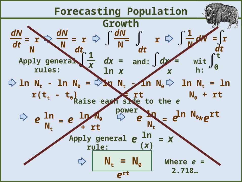
Forecasting Population Growth
dN= r Ndt
dN= r dtN
dN= r dtN
ln Nt - ln N0 = r(tt - t0)
Raise each side to the e power
=e ln N0 + rteln Nt =e ln N0eln Nt rte*
Apply general rule: =e xln (x)
Nt = N0 ert
1dN = r dt
N
Apply general rules:1dx = ln xx and: dx = x with:
0
t
ln Nt - ln N0 = rt ln Nt = ln N0 + rt
Where e = 2.718…
Predator-Prey Dynamics
Victim, V: Predator, P:dV/dt = bvV - dvV - aVP dP/dt = acVP - dpP
We’ll rely on our simulation software (Stella) to examine Vt and Pt
The predator-prey equations are solvable with calculus (integration)i.e., can obtain equations to forecast Vt and Pt at any time
…but the math is pretty ridiculous
BUT, without simulating, we can learn something general about howpredators and prey interact by “solving equations at equilibrium”
i.e., we can derive equations that tell us the abundance of predators and prey at steady-state (i.e., abundance not changing through time)
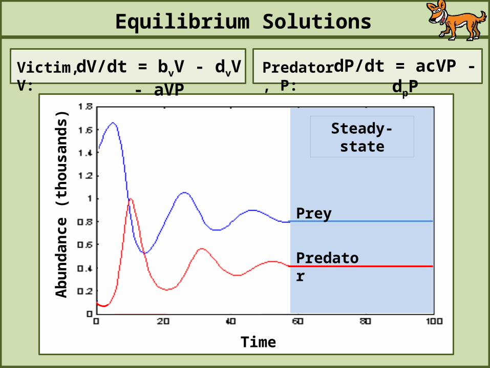
Equilibrium Solutions
Victim, V: Predator, P:dV/dt = bvV - dvV - aVP dP/dt = acVP - dpP
Prey
Predator
Abu
ndan
ce (t
hous
ands
)
Time
Steady-state
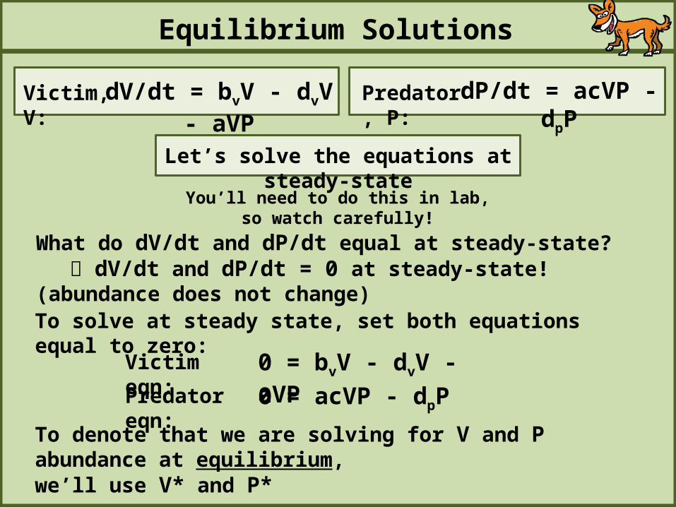
Equilibrium Solutions
Victim, V: Predator, P:dV/dt = bvV - dvV - aVP dP/dt = acVP - dpP
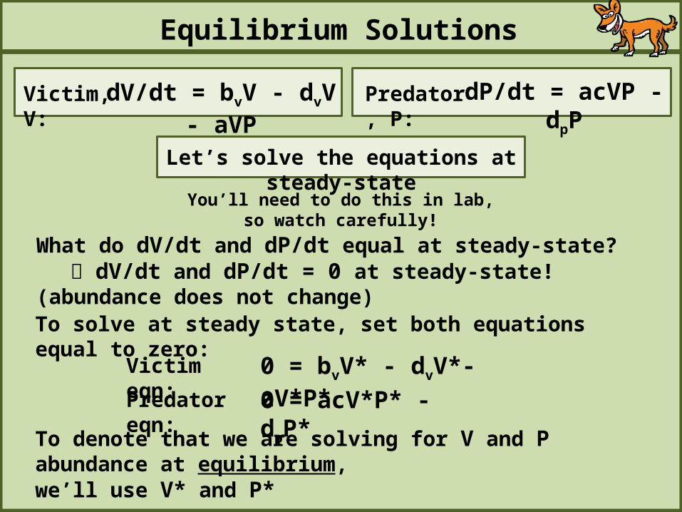
What do dV/dt and dP/dt equal at steady-state? dV/dt and dP/dt = 0 at steady-state! (abundance does not change)
You’ll need to do this in lab, so watch carefully!
Let’s solve the equations at steady-state
To solve at steady state, set both equations equal to zero:
0 = bvV - dvV - aVP0 = acVP - dpP
Victim eqn:
Predator eqn:
To denote that we are solving for V and P abundance at equilibrium,we’ll use V* and P*
Equilibrium Solutions
Victim, V: Predator, P:dV/dt = bvV - dvV - aVP dP/dt = acVP - dpP
What do dV/dt and dP/dt equal at steady-state? dV/dt and dP/dt = 0 at steady-state! (abundance does not change)
You’ll need to do this in lab, so watch carefully!
Let’s solve the equations at steady-state
To solve at steady state, set both equations equal to zero:
0 = bvV* - dvV*- aV*P*0 = acV*P* - dpP*
Victim eqn:
Predator eqn:
To denote that we are solving for V and P abundance at equilibrium,we’ll use V* and P*
Equilibrium Solutions
Victim, V: Predator, P:dV/dt = bvV - dvV - aVP dP/dt = acVP - dpP
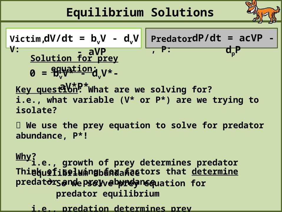
Solution for prey equation:
0 = bvV* - dvV*- aV*P*
Key question: What are we solving for?i.e., what variable (V* or P*) are we trying to isolate?
We use the prey equation to solve for predator abundance, P*!
Why?
Think of solving for factors that determine predator and prey abundancei.e., growth of prey determines predator equilibrium abundance
So we solve prey equation for predator equilibrium
i.e., predation determines prey equilibrium abundance So we solve predator equation for prey equilibrium
Equilibrium Solutions
Victim, V: Predator, P:dV/dt = bvV - dvV - aVP dP/dt = acVP - dpP
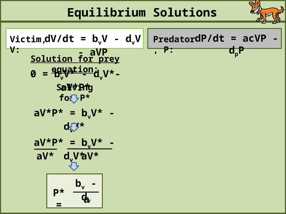
Solution for prey equation:
0 = bvV* - dvV*- aV*P*Solving for P*
aV*P* = bvV* - dvV*
aV* aV*aV*P* = bvV* - dvV*
a
bv - dvP* =
Equilibrium Solutions
Victim, V: Predator, P:dV/dt = bvV - dvV - aVP dP/dt = acVP - dpP
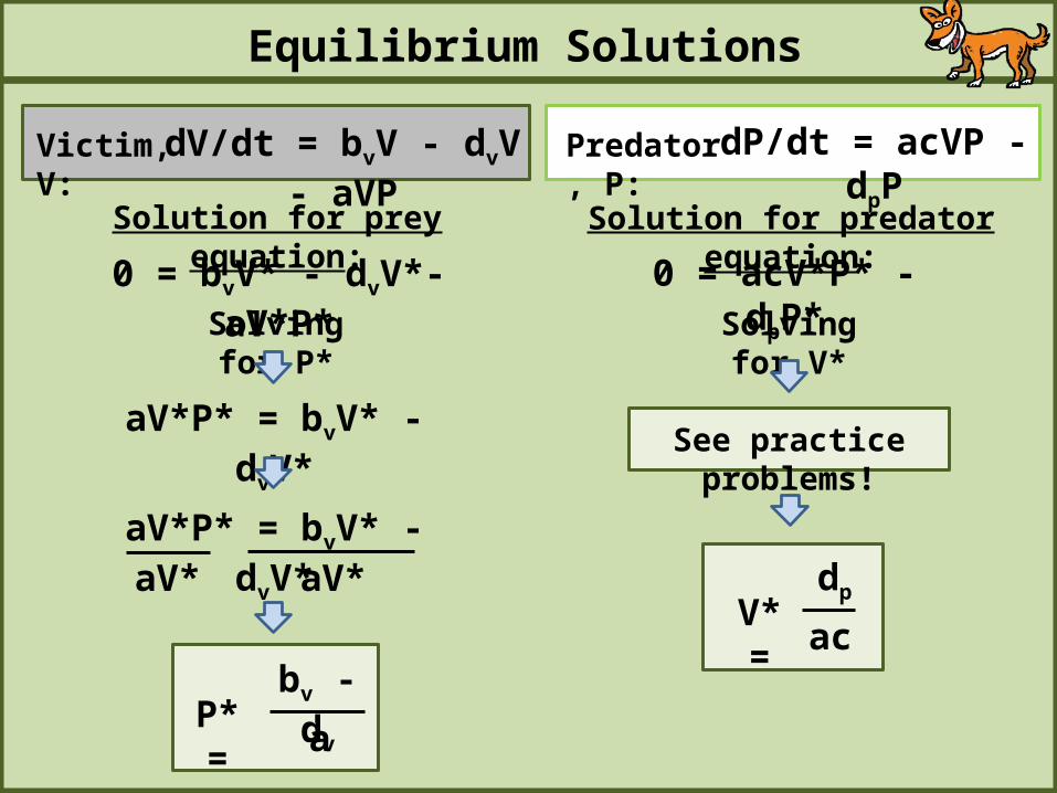
Solution for predator equation:
0 = acV*P* - dpP*Solving for V*
See practice problems!
ac
dpV* =
Solution for prey equation:
0 = bvV* - dvV*- aV*P*Solving for P*
aV*P* = bvV* - dvV*
aV* aV*aV*P* = bvV* - dvV*
a
bv - dvP* =
Equilibrium Solutions
Victim, V: Predator, P:dV/dt = bvV - dvV - aVP dP/dt = acVP - dpP
a
bv - dvP* =
Equilibrium predatorabundanceac
dpV* =
Equilibrium prey abundance
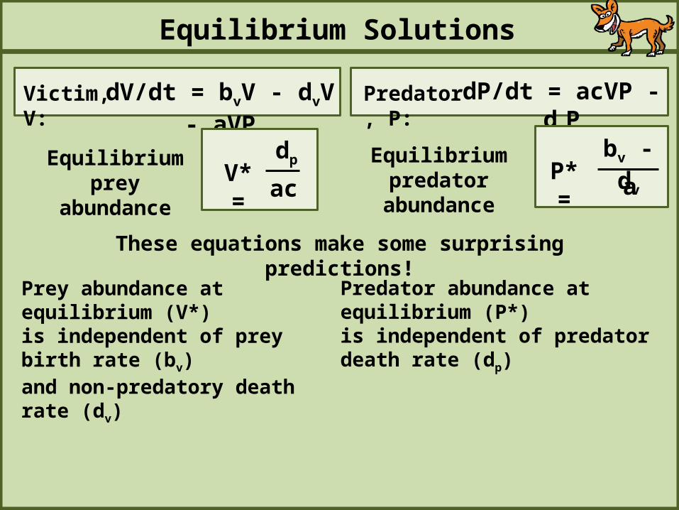
These equations make some surprising predictions!
Prey abundance at equilibrium (V*)is independent of prey birth rate (bv)and non-predatory death rate (dv)
Predator abundance at equilibrium (P*)is independent of predator death rate (dp)
Equilibrium Solutions
Victim, V: Predator, P:dV/dt = bvV - dvV - aVP dP/dt = acVP - dpP
a
bv - dvP* =
Equilibrium predatorabundanceac
dpV* =
Equilibrium prey abundance
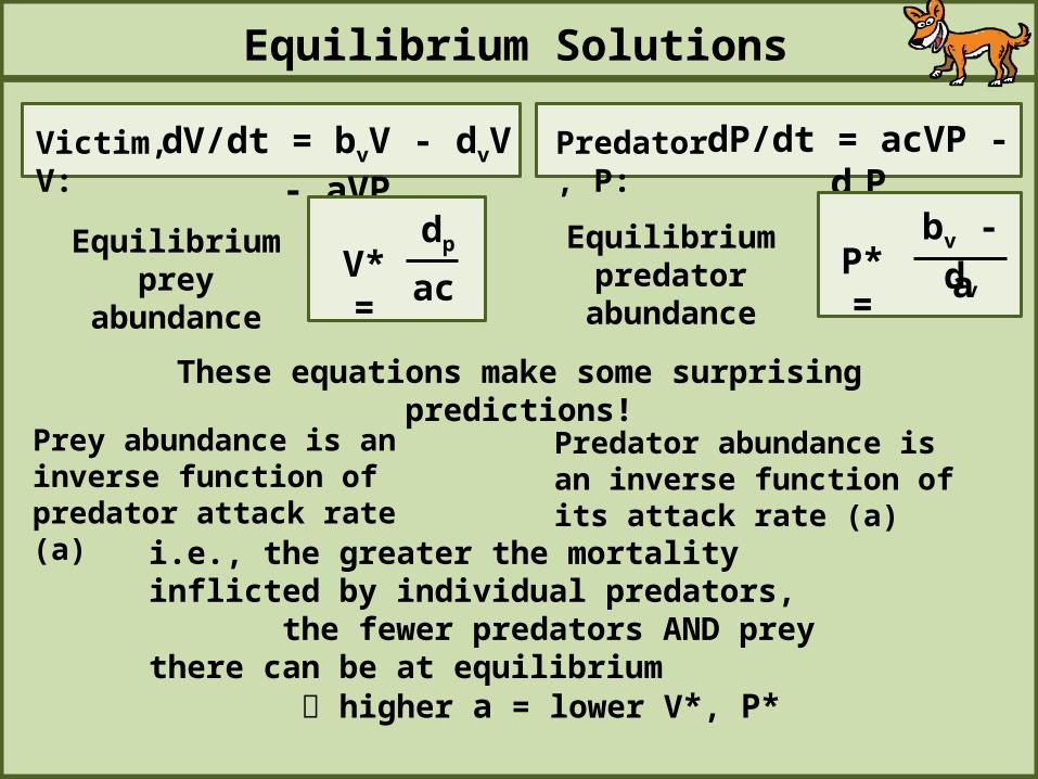
These equations make some surprising predictions!
i.e., the greater the mortality inflicted by individual predators, the fewer predators AND prey there can be at equilibrium higher a = lower V*, P*
Prey abundance is an inverse function of predator attack rate (a)
Predator abundance is an inverse function of its attack rate (a)
Equilibrium Solutions
Victim, V: Predator, P:dV/dt = bvV - dvV - aVP dP/dt = acVP - dpP
a
bv - dvP* =
Equilibrium predatorabundanceac
dpV* =
Equilibrium prey abundance
These equations make some surprising predictions!
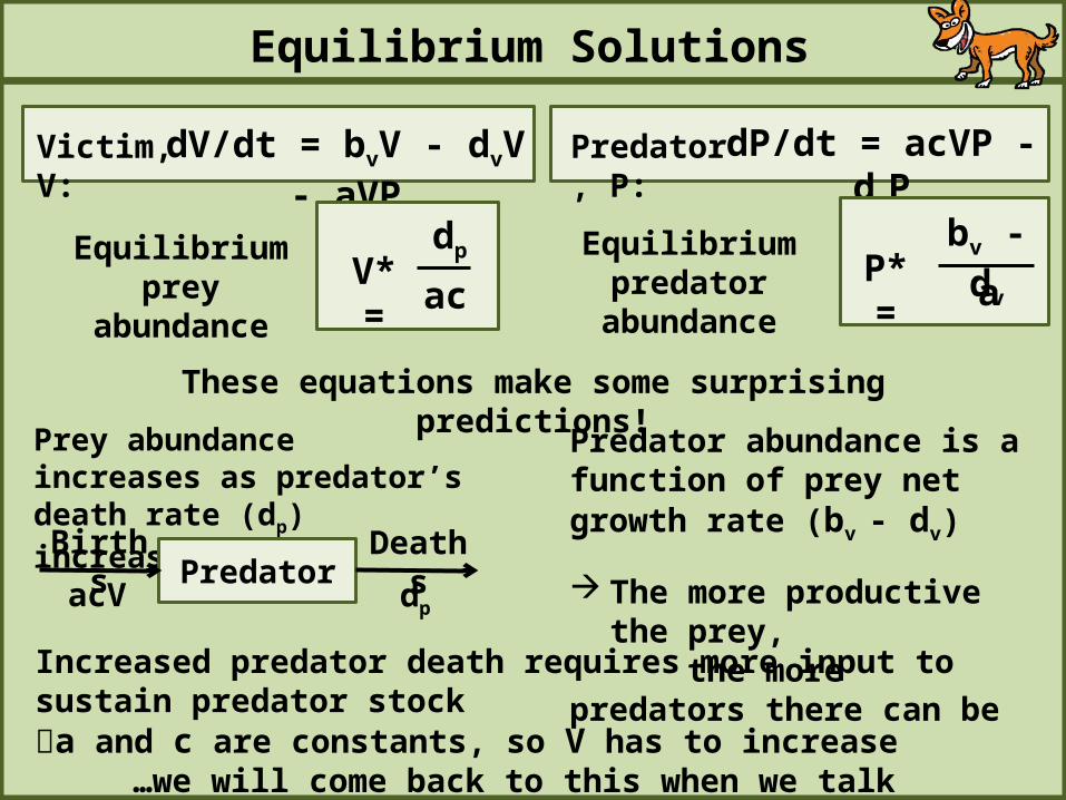
Prey abundance increases as predator’s death rate (dp) increases
Predator abundance is a function of prey net growth rate (bv - dv)
The more productive the prey, the more predators there can be
PredatorBirths Deaths
dpacV
Increased predator death requires more input to sustain predator stocka and c are constants, so V has to increase …we will come back to this when we talk about competition
Equilibrium Solutions
Victim, V: Predator, P:dV/dt = bvV - dvV - aVP dP/dt = acVP - dpP
a
bv - dvP* =
Equilibrium predatorabundanceac
dpV* =
Equilibrium prey abundance
These equations make some surprising predictions!
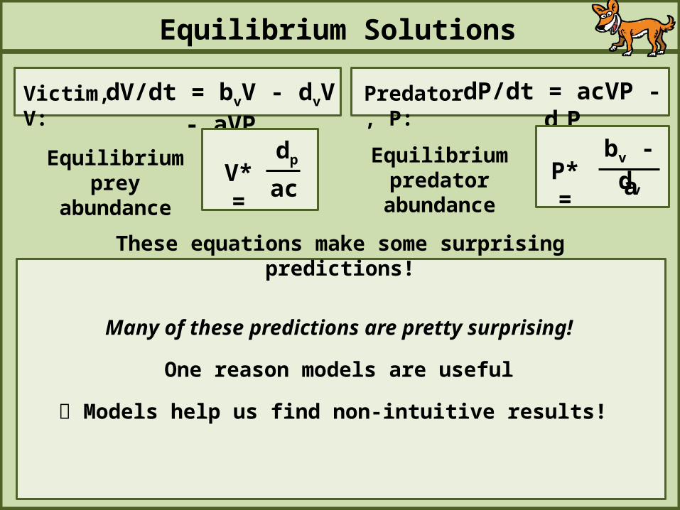
Many of these predictions are pretty surprising!
One reason models are useful
Models help us find non-intuitive results!
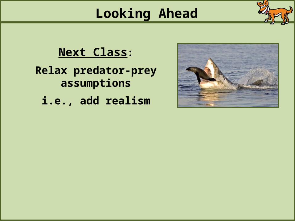
Looking Ahead
Next Class:
Relax predator-prey assumptions
i.e., add realism


![FW364 Ecological Problem Solving Lab 4: Blue Whale Population Variation [Ramas Lab]](https://img.pdfslide.net/doc/110x75/56649e365503460f94b263e5/fw364-ecological-problem-solving-lab-4-blue-whale-population-variation-ramas.jpg)
