Embed Size (px)
Citation preview
INSTITUT NATIONAL DE LA STATISTIQUE ET DES ÉTUDES ÉCONOMIQUES
Série des documents de travail de la Direction des Etudes et Synthèses Économiques
AVRIL 2001
We would like to thank Bruno Crépon for support. We are also grateful to Bernard Salanié, Guy Laroque, Stéphane Grégoir and Jean-Pierre Laffargue for helpful comments. All remaining errors are ours. We also
thank participants at the International Conference on Panel Data held in Geneva in June 2000.
_____________________________________________
* Département des Etudes Economiques d’Ensemble - 15, bd Gabriel Péri - BP 100 - 92244 MALAKOFF CEDEX
** CEPREMAP - 142, rue du chevaleret - 75013 PARIS et London School of Economics
Département des Etudes Economiques d'Ensemble - Timbre G201 - 15, bd Gabriel Péri - BP 100 - 92244 MALAKOFF CEDEX - France - Tél. : 33 (1) 41 17 60 68 - Fax : 33 (1) 41 17 60 45 - E-mail : [email protected] - site web INSEE : http//www.insee.fr
Ces documents de travail ne reflètent pas la position de l’INSEE et n'engagent que leurs auteurs. Working papers do not reflect the position of INSEE but only their author's views.
G 2001 / 05
Testing the augmented Solow growth model: An empirical reassessment using panel data
Cédric AUDENIS * Pierre BISCOURP *
Nathalie FOURCADE * Olivier LOISEL **
2
Testing the augmented Solow growth model: An empirical reassessment using panel data
Abstract We estimate a conditional convergence equation derived from an augmented Solow model where human capital is defined as skilled labour. We implement Generalized Method of Moments (GMM) estimators on a panel of countries. Estimation is carried out on the model in levels instrumented by the lagged first differences of the explanatory variables. We argue that using GMM estimators on the first differenced equation, as was previously attempted, is inappropriate as lagged levels of regressors provide weak instruments for current first differences. Using Asymptotic Least Squares, we check that the GMM estimates for structural parameters are consistent with the restrictions imposed by the model under the classical assumption of constant speed of convergence. We find that countries cover half the distance to their steady state in 16 years. Nonlinear estimations carried out under the assumption of endogenous speed of convergence do not validate the Solow model, whose theoretical predictions as to the dependence of the speed of convergence on structural parameters appear to be at best fragile.
Keywords: convergence, growth, generalized method of moments, dynamic panel data
Une ré-évaluation du modèle de Solow sur données de panel
Résumé
Nous estimons sur un panel de 77 pays une équation de convergence conditionnelle, dérivée d’un modèle de Solow « augmenté » dans lequel le capital humain est défini comme le stock de travailleurs qualifiés. Afin de corriger des biais d’hétérogénéité inobservée et de simultanéité, nous utilisons la Méthode des Moments Généralisés. Nous montrons que la méthode traditionnelle consistant à estimer l’équation en différences premières en l’instrumentant par les niveaux passés des variables explicatives est ici inappropriée parce que les valeurs retardées des régresseurs sont des instruments faibles. Nous réalisons en conséquence l’estimation sur le modèle en niveau instrumenté par les différences premières retardées. A l’aide des Moindres Carrés Asymptotiques, nous vérifions que les coefficients estimés par cette méthode sont cohérents avec les restrictions théoriques imposées par le modèle sur les paramètres structurels, sous l’hypothèse standard de vitesse de convergence constante. Nous trouvons que les pays couvrent la moitié de la distance qui les sépare de leur état stationnaire en 16 ans. Les estimations non-linéaires menées sous l’hypothèse de vitesse de convergence endogène - pleinement cohérente avec le modèle théorique - ne permettent pas de trancher quant à la validité du modèle de Solow.
Mots-clés : convergence, croissance, méthode des moments généralisés
JEL classification : O41, O47
3
Introduction
The Solow model [1956] is generally viewed as a dinosaur in today’s endogenous growth literature. Yet, it has won the status of standard growth model for international institutions’ economists, because of its very simplicity which entails simple predictions. Considering data on macroeconomic growth have obvious limits, because the number of observations as well as the number of well-measured variables are scarce, this simplicity is synonymous of robustness: one may only hope to find empirically significant effects for first-order phenomena well captured by the basic Solow theoretical framework.
Several competing lines of research have developed during the last decade in order to assess the validity of the Solow model. One of them focuses on the issue of parameter heterogeneity across groups of countries and the importance of nonlinearities in the growth process (see for instance Quah [1997] and Temple [1999] for a review of the recent literature on the topic). Another approach takes a different view and postulates that the parameter homogeneity assumption, considered as an approximation to real situations, extends the possibilities of econometric estimation by allowing the use of panel data. In this paper, we follow the latter approach, arguing (see Temple [1999] for a detailed discussion) that both lines of research are worth following, as they point to complementary issues on the matter of explaining the process of growth. We do so because previous attempts seem to us not to have exploited all the methodological tools available in the field of the econometrics of panel data.
Following the line of research initiated by Mankiw, Romer and Weil [1992], we concentrate on the issue of convergence: the simple Solow model predicts that economies sharing the same saving rate and population growth rate should eventually converge to the same long run path given initial conditions. The issue of whether such a crude theoretical framework may be validated by the data has given rise to a huge empirical literature, spurred by the availability of the Summers and Heston [1988] dataset. Results so far appear to be inconclusive. Let us first summarize them briefly before presenting the methodological improvements we think may be made to this approach.
Mankiw, Romer and Weil [1992] proposed a test of the augmented1 Solow model based on the estimation of a convergence equation. Their results were criticized, however, as doubts were shed on the use of Ordinary Least Squares (OLS) to estimate a dynamic equation on cross section data (Islam [1995]). Indeed, OLS yields unbiased estimates only as long as residuals are uncorrelated with explanatory variables. This condition may hold for the static steady state equation estimated by Mankiw Romer and Weil, as the endogeneity of regressors with respect to productivity shocks remains subject to discussion. However, estimating a static equation rests on the assumption that economies are likely to have reached their steady state within the estimation period. A conditional convergence framework is both more general and more convincing. OLS, however, is no more an appropriate method for estimating a convergence equation2: it seems unreasonable to extend the assumption of absence of correlation between the residual and exogenous regressors to the lagged endogenous variable, as the latter contains unobserved individual effects. Residuals derived from the Solow model in particular contain a country specific initial level of technology likely to be correlated with initial GDP levels.
In order to deal with this unobserved heterogeneity issue, Islam [1995] advocates the use of the Chamberlain3 estimation method. However, the Π matrix approach he uses, as well as Knight, Loayza, and Villaneuva [1993], focuses on the issue of the endogeneity of regressors with respect to individual effects, and does not tackle the problem of the simultaneity of investment rates and productivity shocks.
1 i.e. including human capital accumulation. 2 i.e. containing an autoregressive term. 3 For a presentation of the P matrix approach, see Chamberlain [1984].
4
Caselli, Esquivel and Lefort [1996] therefore implements Generalized Method of Moments (GMM) panel data estimators. They estimate a first differenced convergence equation instrumented by lagged levels of explanatory variables. This has indeed become the standard approach since Arellano and Bond’s [1991] seminal paper. Their results prove imprecise, which seems to raise doubts as to the very possibility to validate a simple human capital augmented Solow model.
We use both Mankiw, Romer and Weil [1992] and Caselli, Esquivel and Lefort [1996] as starting points for our empirical analysis of the issue of convergence. The former provides the general theoretical framework, used by all followers in this literature, which we shall discuss and adapt. The latter provides what seems to us to be the most rigorous econometric treatment available in the existing literature. This paper must be seen as an attempt to provide a more rigorous methodology on both aspects in order to assess whether the inconclusive results obtained so far (in this respect, Caselli, Esquivel and Lefort [1996] will be our benchmark) are due to the inadequacy of the augmented Solow model, to methodological problems within the line of research followed (that of panel data estimation under the assumption of homogenous technological parameters), or to the very approach. It must therefore be seen as a twofold methodological contribution.
Our estimation strategy first differs from previous attempts. We implement GMM panel data estimators on a model in levels instrumented by past first differences of the explanatory variables. This approach is valid, as Arellano and Bover [1995] have shown, under the additional identifying assumption of constant correlation between explanatory variables and the individual effect. We focus on this estimation strategy because given the high degree of autocorrelation of explanatory variables in a panel framework, lagged differences of regressors provide better instruments for current levels than lagged levels do for current first differences.
We also propose an alternative way of taking into account human capital accumulation, traditionally modelled by analogy with physical capital: since Mankiw, Romer and Weil [1992] a « saving rate » in human capital is applied to national income, the measure of this saving rate being provided by rates of schooling weighted by shares of population of schooling age. This approach is questionable since the very definition of human capital remains inexplicit. We define human capital as skilled labour. We compute a rate of investment in human capital derived from the share of total population who has attained a secondary level. In order to guarantee the theoretical consistency of the model, we apply this rate of investment to the country’s population as opposed to its GDP.
Our estimates of structural parameters under the traditional assumption of constant speed of convergence yield plausible values: the elasticity of production to physical capital roughly equals 30%. We find a half-life of convergence equal to 16 years4. Our model is overidentified in that we estimate more coefficients than we have structural parameters. Using Asymptotic Least Squares, we prove that the constraints implied by the model are not rejected. It turns out that these results do not require the use of all past first differences as instruments.
Testing the Solow model under the assumption of constant speed of convergence is handy because it relies on linear econometrics methods. However, it is not theoretically consistent as deriving a convergence equation from an augmented Solow model yields an endogenous expression for the speed of convergence. We test a more general model where we allow for the presence of both a constant and an endogenous term in the speed of convergence. The endogenous component appears to be significant yet weakly consistent with the data, while the constant one appears to be significant, in contradiction with the model. We conclude that our econometric methodology allows to obtain sharp improvements in the accuracy of the estimated parameters, but that these results do not allow to conclude to the full consistency of the theoretical model with the data. They do not
4 Thus, we find convergence to be faster than was estimated by Mankiw, Romer and Weil, yet slower than in
Caselli, Esquivel and Lefort’s study.
5
validate the use of the assumption of constant speed of convergence either, as the endogenous component of the latter is significant.
The remainder of the article is organized as follows. Section 1 briefly reviews previous attempts, points to their limits and presents our estimation strategy. The Solow convergence equation based on our modelling of human capital accumulation is derived in section 2. We then discuss our results under both assumptions of constant and endogenous speed of convergence.

6
7
Failures to validate the Solow model: wrong model or poor methodology?
Mankiw, Romer and Weil’s [1992] validation of the Solow model rests on strong econometric assumptions Mankiw, Romer and Weil (henceforth MRW) proposed in 1992 a simple test of the Solow model. The authors consider the basic textbook Solow model as well as an « augmented » version which includes human capital as an input of the production function. Their framework allows for conditional convergence, where saving and population growth (and consequently the long run path) are exogenous and idiosyncratic.
They first estimate a static equation under the assumption that the economy reaches its steady state within the period 1960-1985. Then, turning to conditional convergence, they estimate an autoregressive model. The first estimation by OLS is only valid if the regressors are uncorrelated with the residuals. Recall however that using OLS to estimate an autoregressive model on individual data is poor methodology leading to a downward bias on the estimate of the speed of convergence (Islam [1995]).
The model
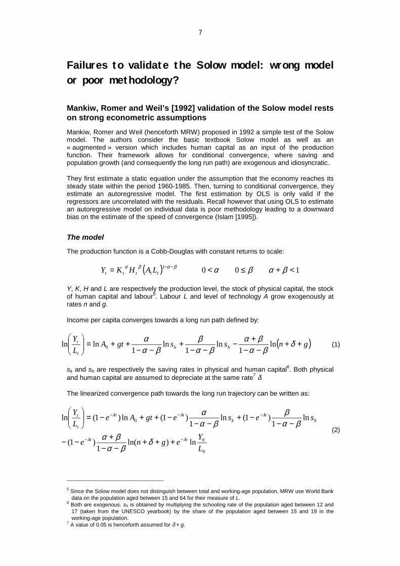
The production function is a Cobb-Douglas with constant returns to scale:
( ) 1001 <+≤<= −− βαβαβαβαttttt LAHKY
Y, K, H and L are respectively the production level, the stock of physical capital, the stock of human capital and labour5. Labour L and level of technology A grow exogenously at rates n and g.
Income per capita converges towards a long run path defined by:
( )gnssgtALY
hkt
t ++−−
+−−−
+−−
++=
δ
βαβα
βαβ
βαα ln
1ln
1ln
1lnln 0 (1)
sk and sh are respectively the saving rates in physical and human capital6. Both physical and human capital are assumed to depreciate at the same rate7 δ.
The linearized convergence path towards the long run trajectory can be written as:
0
0
0
ln)ln(1
)1(
ln1
)1(ln1
)1(ln)1(ln
LYegne
sesegtAeLY
tt
ht
ktt
t
t
λλ
λλλ
δβα
βαβα
ββα
α
−−
−−−
+++−−
+−−
−−−+
−−−++−=
(2)
5 Since the Solow model does not distinguish between total and working-age population, MRW use World Bank
data on the population aged between 15 and 64 for their measure of L. 6 Both are exogenous. sh is obtained by multiplying the schooling rate of the population aged between 12 and
17 (taken from the UNESCO yearbook) by the share of the population aged between 15 and 19 in the working-age population.
7 A value of 0.05 is henceforth assumed for δ + g.
8
where ( )( )λ α β δ= − − + +1 n g is the speed of convergence8.
Estimation by Ordinary Least Squares
Both static steady state equation (1) and convergence equation (2) are estimated using the Summers and Heston dataset. Estimating equation (1) rests on the assumption that all countries have reached their steady state in 1985, starting from 1960. Steady states are idiosyncratic and defined by the corresponding values of n, sk and sh, computed as the average of these variables over the period 1960-19859.
Equation (2) by contrast allows for only partial convergence. Note however that estimation is carried out under the assumption that the speed of convergence λ may be estimated in the same way as technological parameters α and β. This is indeed the traditional approach to statistical convergence tests. However, one should be clear as to the goals assigned to the estimation of equation (2): if such estimations aim at providing a test of the Solow model, then all theoretical relationships derived from the model should be taken into account, in particular the endogenous expression of the speed of convergence. We turn to this criticism in more details in section 3, and focus in this section on the discussion of the estimation method used by MRW.
The equation residual reflects initial levels of technology: MRW split up the term ( ) ln1 0− −e Atλ appearing in equation (2) into a constant a and a country specific
effect εA: ( ) ln1 0− = +−e A atA
λ ε .
Specifying the model means making identifying assumptions on the properties of this residual. εA is assumed by MRW to be not only independent and identically distributed, but also orthogonal to all explanatory variables. This strong assumption allows them to use OLS.
Indeed, the static model described by equation (1) yields parameter estimates consistent with plausible values (α = β = 0.3). The convergence equation (2), however, leads to far less satisfactory results: the estimates for α, β and λ respectively take the values 0.5, 0.2 and 0.014, the latter implying a fairly long half-life of convergence equal to 52 years10.
Islam [1995] argues that this very low speed of convergence was to be expected, since the non-observed individual disturbance term εA is likely to be correlated with the initial state of the economy: as a result, OLS estimators are biased, even under the assumption of exogenous steady state explanatory variables, since the lagged endogenous variable is affected by the individual shock.
The panel data approach, once promising, yet apparently inconclusive Islam [1995] advocates to this end the use of panel data. However, the Chamberlain method he uses does not tackle the issue of simultaneity. Caselli, Esquivel and Lefort [1996] (henceforth CEL) implements Generalized Method of Moments estimators on panel data in order to deal with both sources of bias. Their results prove inconclusive, which casts doubts on the validity of the whole approach.
8 For a proof, see Mankiw, Romer and Weil [1992] or the appendix of this paper in a more general case. 9 t is therefore a constant equal to 25, since the estimation period is 1960-1985. 10 i.e. it takes 52 years for half the gap to the steady state to vanish.

9
Caselli, Esquivel and Lefort’s approach [1996]:
The estimated equation
CEL extend the theoretical approach of MRW to a panel framework. They divide the 1960-1990 period into six five-year sub-periods. This allows to use panel data. The number of cross section units is large relative to the number of periods, which is the usual condition for panel data estimators to perform well.
Equations (1) and (2) become11:
itithkit
it gnssaLY
ititεδ
βαβα
βαβ
βαα +++
−−+−
−−+
−−+=
)ln(
1ln
1ln
1ln (1’)
( ) ( )
( ) ( )
ln ln ln ln
ln
YL
a e YL
e s e s
e n g
it
it
it
it
it
k
it
h
it it
= +
+ −
− −+ −
− −
− − +− −
+ + +
− −
−
− −
−
5 1
1
5 5
5
11
11
11
λ λ λ
λ
αα β
βα β
α βα β
δ ε (2’)
Again, CEL ignore the theoretical definition of the speed of convergence and stick to the traditional assumption that λ is constant across time and countries.
CEL transpose the MRW framework to each sub-period, so that one steady state is then available for each sub-period. This (now temporary) steady state undergoes changes from one sub-period to the next, caused by stochastic shocks assumed to be exogenous (i.e. independent of the past states of the economy). Because economies are unlikely to achieve full convergence towards their local steady state within each sub-period, equation (1’) becomes irrelevant and only equation (2’) remains to be estimated.
ln(n+g+δ), ln(sk) and ln(sh) at time t are computed as the average of these quantities over the sub-period beginning in t. Note that contrary to MRW who base their definition of steady state on the average of explanatory variables over the convergence period, CEL use their current value: this implies that convergence takes place between t-1 and t towards a steady state defined by the vector of explanatory variables at date t.
Identifying restrictions
Residuals are decomposed into the following way:
ε η νit i t itu= + +
where ui and ηt correspond respectively to the individual and time effects12.
For an autoregressive equation, the OLS estimator is biased because the lagged endogenous variable included in the set of regressors is correlated with ui (unobserved heterogeneity bias).
11 Due to the panel structure of the data, equation residuals now include time effects as well as individual
effects. 12 CEL eliminate the time effect by centering the data by their mean over the sub-period. Note that unlike the
first two components of the residual, νit can not be derived from the model without further assumptions. Assume for instance that the level of technology lnA is randomly distributed across countries and through time, its expectation at time t being given by lnA0 + gt, we have : lnAit = lnAi0 + gt + vit.

10
Another source of bias stems from the likely correlation between νit and the explanatory variables (endogeneity bias).
In order to deal with both sources of bias, CEL use the Generalized Method of Moments (GMM) under the assumption of weak exogeneity13. The economic intuition behind the latter is that current explanatory and endogenous variables are not correlated with future shocks, but may be correlated with past or current shocks. Indeed, one does not expect an unforecasted climatic shock at date t+1 to influence GDP, the population growth rate or the saving rates at date t. However, it is far less clear that this hypothesis of independence should also apply to current and past shocks.
Explanatory variables taken previous to the shock are therefore instruments. Current and future values however are not included in the set of instruments, as they are likely to be correlated with current shocks.
In practice CEL estimate the equation in first differences using the explanatory variables in levels lagged twice or more as instruments. This has become the standard approach since Arellano and Bond’s seminal paper (1991).
Results: a relative failure
The estimation of the model leads to a negative β and to an implausible value for α (0.49), the speed of convergence λ being estimated at around 10% which implies a half life of convergence equal to 7 years. If CEL’s methodology is to be taken seriously, these results undoubtedly argue against the Solow model.
An alternative econometric strategy The relevance of CEL’s methodology may however be questioned for two reasons:
• Their modelling of human capital, inherited from MRW, relies on a perfect symmetry between the processes of human and physical capital accumulation. This simplifies calculations but does not account for the singularity of human capital. This calls for an alternative modelling (see section 2).
• Estimating equation (2) written in first differences using instruments in levels may not be appropriate considering the type of variables we are dealing with.
We illustrate here the latter point.
Estimating the convergence equation in levels, instrumenting by lagged first differences performs better under serial correlation of some regressors.
Recall that two properties are required for variable Z to instrument explanatory variable X properly:
- Z must not be correlated with the residual of the model
- Z must be correlated with X, more precisely the coefficient of the regression of X on Z must be significantly different from zero. Whenever several instrumental variables are available, the most efficient (i.e. which leads to a minimal variance for the instrumental variables (IV) estimator) is the one best correlated with the explanatory variable.
13 Namely ( ) ( ) ( )E x u E x t s s tit i it is≠ = ∀ >0 0, , /ν . Recall that the OLS estimator is biased even on the
model written in first differences as long as the estimated equation is autoregressive.
11
Following Blundell & Bond [1998], we argue that lagged levels of explanatory variables are weak instruments for their first differences, whereas lagged first differences are appropriate instruments for levels, when the X variable exhibits strong enough serial correlation. We show this in the simple case where X follows an autoregressive process of order one: using lagged first differences of X to instrument current levels leads to a smaller variance of the IV estimator than using lagged levels of X to instrument current first differences.
Start from the following fixed effect model:
Y X Uit it i it= + +β ε
with V it( )ε = Σ Ι2 and E X U E Xit i it it( ) , ( )≠ ≠0 0ε .
Assume X follows an autoregressive process of order one:
X X uit it i it= + +−ρ ω1
where ρ <1 , ω is a white noise (variance σ2). Under these assumptions and the following stationarity condition
( ) ( ) ( )cov , cov , , ''X u X u t tit i it i= ∀
it is straightforward to obtain:
( )( )
V XV ui( ) =
−+
−σ
ρ ρ
2
2 21 1
V X( )∆ =+
21
2σρ
We want to compare the performances of two competing instrumental variable estimators of β :
• The estimator based on the model written in first differences, where the explanatory variable lagged twice provides an instrument for the current first difference
• The estimator based on the model in levels, where the first difference of the explanatory variable lagged once instruments the current level of X.
More precisely, we want to evaluate the ratio of the variances of both estimators as a function of the inertia of the process that generates X.
The asymptotic variances of the corresponding IV estimators have the following expressions:
( )itit
itit
levIV XXN
XVVV
,cov)(
)()ˆ(1
21
−
−
∆∆
= ηβ
( )itit
itit
difIV XXN
XVVV
∆∆=
−
−
,cov)(
)()ˆ(2
22ηβ
12
where itiit U εη +=
Let Q denote the ratio of both quantities:
( )( ) )(
)(,cov
,cov)(
)(
2
1
12
22
−
−
−
− ∆∆
∆∆
=it
it
itit
itit
it
it
XVXV
XXXX
VV
Qη
η
The ratio of the squared covariances involved in the previous expression is easily shown to be one.
Q has therefore the following expression:
( )( )Q
V UV u
i
i
=+
+− −
++
ΣΣ
2
2
2
222
11 1 1
σρρ ρ
σρ
Let us characterize Q in terms of ρ and a parameter α equal to the ratio of the variance of the individual effect to the variance of the perturbation within the process generating X:
( )ασ
=V ui
2
Assume further for simplicity that this ratio is identical for the individual effect and the perturbation involved in the estimated equation. One then obtains a simple expression for Q:
( )( )
( )Q =+ −
− + +1 1
1 1
2α ρρ α ρ
The distribution of Q given ρ and α is shown in Figure 1. When X exhibits no serial correlation (i.e. ρ = 0 ), Q is equal to one, in other words both estimators perform equally well or badly. However, for larger values of ρ , which are to be expected with macroeconomic data, the ratio of variances decreases sharply, all the more so when α is large, which is also to be expected.

13
Figure 1 - Ratio of the variances of both instrumental variables estimators in terms of ρ and α
0
0.2
0.4
0.6
0.8
1Rho
24
68
10
Alpha
0
0.25
0.5
0.75
1
Q
0
0.2
0.4
0.6
0.8
1Rho
24
68
10
Alpha
The previous considerations help understand why estimations of the first-differenced model perform badly when explanatory variables exhibit strong serial correlation. They also point to a remedy to this problem, which consists in estimating equation (2) in levels using first differenced explanatory variables lagged once or more as instruments.
However, equation (2’) written in levels contains the individual effect ui, which implies that orthogonality conditions derived from this specification are only valid under the additional condition ( )E x u tit i∆ = ∀0 . Arellano and Bover [1995] first pointed that a sufficient condition for this equality to hold is the following stationarity assumption:
( ) δ=iituxE
i.e. the correlation between the individual effect and the explanatory variables is not time dependent. This condition is intermediate between the absence of fixed effect (δ = 0) and the less demanding assumption made by Arellano and Bond [1991] and used by CEL (δ = f(t)).
Note that this assumption of constant correlation between explanatory variables such as saving rates, and the individual effects, may be invalid if the countries starting from a low technological level turn out to be the ones whose saving rates grow fastest (i.e. absolute convergence takes place). However, most of this absolute convergence has been taking place between groups of countries (such as the NIC and the OECD, the former tending to catch up with the latter). Hence, we deal with this criticism by centering all variables by date and group of countries, which is equivalent to adding a complete set of crossed
14
group and time dummies14. As in our framework country specific effects are deviations from group averages, the stationarity assumption may still be considered to hold.
The conditions under which the lagged first differences of the endogenous variable may be used as instruments can be derived by iterating equation (2’) in levels. Blundell and Bond [1998] show that this is the case if the generating process described by equation (2’) is convergent, goes back to infinity, and if the stationarity and weak exogeneity assumptions hold, as well as the absence of autocorrelation for ν.
We proceed as follows:
• We start by checking for the absence of autocorrelation on the residual ν of the model in levels. Crossing time and group effects reduces the risks of serial correlation on the residual ν (which becomes a deviation from the group’s average shock). There is still a need to test for autocorrelation. As the presence of an individual effect in the overall level residual inevitably makes it serially correlated, we estimate the first differenced equation using the endogenous and the explanatory variables in levels lagged twice or more as instruments. We check for autocorrelation of νit - νit-1 at order one and two. One expects autocorrelation at order one but not at order two if ν is not serially correlated.
• The equation in levels is estimated using the endogenous and the explanatory variables in first differences lagged once or more as instruments. A Sargan test is used to check for the consistency of the set of orthogonality conditions (recall that a Sargan statistics follows a chi-squared with a number of degrees of freedom equal to the excess of orthogonality conditions over the number of parameters of interest).
This discussion finally leads to two theoretical specifications15:
Specification Equation in level at time t Equation in first differences at time t
Available instruments
∆xi1,..., ∆xi,t-1
∆yi1,..., ∆yi,t-1
xi1,...,xi,t-2
yi1,...,yi,t-2
The validity of instruments added to the set of instruments of any specification may be tested by a difference Sargan test: if the additional moment conditions are valid, then the difference between the Sargan statistics follows a χ2 with a number of degrees of freedom equal to the number of additional moment conditions16.
In the next section we present the model we estimate through these specifications.
14 Time effects η are therefore eliminated in the process. We also tackle the issue of « group effects » pointing
to strong observable heterogeneity, for instance between the OECD countries and the Newly Industrialized Countries versus the rest of the world.
15 We have implemented a third specification called System Estimator, first suggested by Arellano and Bover [1995]. It consists in combining both specifications by adding a set of orthogonality conditions derived from the equations in levels, to the ones obtained from the model written in first differences. Results are not displayed here because the relevance of the method can be questioned in our case. Retaining all possible instruments may not be optimal when dealing with a small sample (see Appendix). Moreover, since the relevance of the orthogonality conditions corresponding to the first-differenced model is questionable, adding these conditions to the ones generated by the model in levels is of little interest. Indeed, results with this specification are more satisfactory than with System Estimator.
16 This is valid provided the additional instruments are orthogonal to the initial set of instruments.

15
A Solow model with human capital defined as skilled labour
Defining and measuring human capital Estimating an augmented Solow model has always been a tricky issue since it implies that one has in hand both a clear definition of the rate of investment in human capital, and a measure consistent with the theoretical concept. Previous studies have typically focused on the rate of secondary schooling, weighted by the share of population of schooling age, as this information is readily available from UNESCO for a large sample of countries (see MRW). This approach makes sense since it captures the intuition that the relevant issue when it comes to human capital accumulation is that of improving the available number of skilled workers in the economy.
However, the issue we want to deal with is the consistency of this measure of sh with the theoretical framework it is embedded in. MRW for instance model human capital accumulation by analogy with physical capital: a share sh is assumed to be devoted to human capital accumulation in the same way as a proportion sk of national income is directed towards physical capital accumulation. This analogy is very handy when it comes to solving the model, since it allows one to make use of the symmetry of accumulation equations to derive an extended expression for the convergence path to the steady state, from the simple Solow convergence equation. However, applying a concept of human capital investment based on a rate of schooling to a financial income, may be viewed as dubious. Indeed, one would rather expect the share of education expenditure in GDP as a measure of sh
17.
If one is concerned about modelling human capital accumulation in a way that makes it analogous to physical capital, a better choice for the corresponding concept of « income » would be the amount of total population for whom the decision is to be made at the beginning of every period, whether they should be schooled (i.e. « saved » to increase productivity next period), or not (i.e. « consumed » immediately as unskilled workers).
Contrary to CEL we define the population as the total population (and not only people of working age), since we expect this variable to be better measured. Recall that the Solow model does not distinguish between the two.
We define the stock of human capital by the number of working-age people who have attained the secondary level (this is a proxy for skilled labour). The rate of investment in human capital is then given by the accumulation equation:
H H s N Ht t th
t t+ − = −1 δ
The variation between t and t+1 in the stock of skilled people is due to the difference between the inflow of students graduating from high school, and an exit rate δ assumed to be constant. Note that by definition, sh is applied to the stock of population at a given date. In order to interpret it as an investment rate, one would expect sh to apply to a flow of population eligible for schooling, for instance the number of people aged between 15 and 20 years. Such data are to our knowledge not available. We consequently assume that there is some unobserved variable equal to the share of the 15-20 years in total population, which may vary from one country to another, and for a given country from one date to the next. As this variable is not measured, but is applied in a multiplicative way to the stock of total population, its logarithm ends up in the residual of our equation, either as part of the individual effect or as part of the νit residual.
17 The latter is a poor proxy for human capital investment, since it is polluted by unobserved heterogeneous
efficiency across schooling systems. We therefore focus on their measured output.

16
We calculate our rate of human capital investment sh as follows. We obtain the share Rt of total population Nt that has attained the secondary level at time t from the Barro and Lee dataset. Hence :
s R NN
Rt
h
tt
t
t= − −++
11 1( )δ 18
The model We specify the aggregate production function as:
Y t A t K t H t L t( ) ( ) ( ) ( ) ( )= − −α β α β1
where H(t) and L(t) stand for skilled and unskilled labour and A(t) is technical progress19.
By assumption20 :
N H L= +
We derive the human capital accumulation equation from the definition of sh :
H s N Hh H= −δ
Note that there is no explicit feedback of income on capital accumulation. Recall that the basic Solow model takes the saving rates as given exogenously. We extend this assumption to human capital investment which undergoes exogenous shocks every five years, causing the steady state of the economy to change.
Accumulation equations per head of population are then written:
( )k s y n kk K= − +δ
( )h s n hh H= − +δ
l h= −
As the ratio of output to the stock of physical capital is fairly constant over time, the rates of growth of per head output and per head capital must be identical at the steady state. We also assume that the per head skilled workforce is constant. Note that it follows from our definition of human capital that all variables do not grow at the same rates at the steady state. For this reason, we shall term it « limit trajectory ».
18 Contrary to the other explanatory variables, which are calculated as the means over five years of their annual
logarithm, the rate of investment in human capital is only known every five years from the Barro&Lee data set. This value is assumed to remain constant over the five year period following date t, and its annual equivalent is obtained from this expression divided by five. Moreover, the way sh is computed implies that its value is missing for the most recent period.
19 Recall that in the special case of a Cobb-Douglas function, all forms of technical progress are equivalent. Contrary to MRW and CEL, we start from a macroeconomic production function incorporating a Solow neutral technical change. The reason for this is that we define human capital as skilled labour. Since total population N is now divided into two components, it is no longer natural to model a Harrod neutral technical change and define all variables per efficient unit of labour. We therefore stick to per head values.
20 This is obviously an approximation. If we assume, however, a share of aggregate labour in population constant across time, yet allowed to differ between countries, we only end up adding another individual effect to the residual of our equations. We deal with this effect as before. Alternatively, this approximation can be avoided by using the working-age population as a measure of N. Comfortingly, results are unchanged (results of the estimations using working-age population are not displayed here).
17
The method we use to derive a convergence equation to the limit trajectory defined above i.e. the path followed by per head output to its target when both values are initially different, consists in approximating accumulation equations around a steady state (*) obtained by transforming per head variables into another set of variables which have the property that they are constant when the limit trajectory is reached (as a result, skilled and unskilled labour are invariant by this transformation). We then plug these approximations into the log-differentiated production function and factorize this expression into a first order differential equation whose solution is the convergence path21.
The solution (see appendix for a proof) is given by:
( )ln ln ln *y e y e yt t= + −− −λ λ0 1
( )( )λ α δ= − +1 n *
This solution may be interpreted as follows. If at a given date taken as the origin of time, output per head happens to differ from the steady state implied by the (exogenous) values of saving rates and the growth rate of population for a given country, the Solow model predicts that convergence towards this steady state will take place at the speed λ. More precisely, output per head at any given date t along this convergence process is a weighted average of the initial value y0 and of the steady state value (the « target » of convergence) y*, with the weight on the initial value going to zero when t goes to infinity, the weight on the steady state value conversely going to one, all the more rapidly so if λ is large.
Mankiw, Romer and Weil [1992] estimated this equation for a cross section of countries between 1960 and 1985: in their case y0 denotes output per head in 1960 for a given country, y denotes output per head measured in 1985, and y* is assumed to be the steady state implied by the Solow model, computed by using averages of saving rates and growth rates of population taken over the whole 1960-1985 period. Indeed, under this assumption, the length of time seems to be sufficient to allow full convergence to steady states. One should bear in mind however that the definition of steady state they use is fully arbitrary. Our panel data framework is a generalization of that used by MRW. Convergence, likely to be partial, takes place over five or ten years: y0 denotes output per head at the beginning of any of these periods of convergence, y denotes output per head measured at the end of the period, and y* is assumed to be the steady state implied by the Solow model, computed by using averages of saving rates and growth rates of population taken over the period. Steady states are therefore fully exogenous, as in the MRW framework, but undergo stochastic shocks every five or ten years. The target towards which (partial) convergence takes place during a given period, therefore moves from one period to the next.
Expanding the previous expression using the definition of the steady state, we obtain the following equation, where the parameter τ is introduced to determine the length of the lag on the autoregressive term.
( ) ( )ln ( ) ln ( ) ln ( ) ln( )
( ) ln( ) ln
* * *
*
y e s e s e n
e n s e y
t tk
th
t
t th
t t
= −−
+ −−
− −−
+
+ − − −−
+ − + +
− − −
− −−
11
11
1 11
1 11
5 5 5
5 5
λτ λτ λτ
λτ λττ
αα
βα α
δ
α βα
δ ε
(2’’)
21 Note that this dynamics is one-dimensional. The literature on convergence within the Solow framework has
to make assumptions on the values taken by the rates of depreciation of physical and human capital in order to obtain a factorisation of this dynamics. MRW for instance assumed the equality of both rates. Given our more general model, we must assume that the rate of depreciation of human capital is equal to that of physical capital plus the rate of growth of output on the limit trajectory.
18
Equation (2’’) describes the path followed by a country while converging towards its steady state. Theory does not, however, imply any particular value for this convergence period, as identical values should be obtained for α, β and λ whatever the spell of time considered. For the sake of econometric estimation, one should retain any length of time τ allowing the economy to move forward to its target (its steady state on the corresponding sub-period) in a sufficiently clear way, while short enough not to imply too big a loss in terms of time series observations.
Choosing τ =1 - like CEL - makes sense if it can be assumed that convergence appears to take place significantly over a period of five years, and can therefore be subject to measurement on this length of time. τ =2 is otherwise a safer bet. For an estimation in levels, the latter is more appropriate, since inertia is a lot stronger for GDP in levels than it is for growth rates.
Following MRW, we assume in both cases that our economy converges between t-τ and t towards a steady-state that may be approximated by the average of the relevant variables on this spell of time22. A natural choice associated with τ for any given steady state
variable x is then: ( )xt mean xt xt* , ...,= − τ .
22 As the human capital variables are missing for the most recent period because they are defined in a
recursive equation involving the future, averages for these variables are computed over all available dates.
19
Testing the Solow model
MRW and CEL rely on two methods in order to assess the consistency of the Solow model with the data.
As mentioned in section 1, they first use the estimates of the coefficients to compute values for α and β. These estimates are then compared to widely acknowledged values for these parameters. This can hardly be considered a statistical test of the model.
The prediction of the model that the sum of the coefficients of ln sitk and ln sit
h should be the opposite of the coefficient on ln( )n git + +δ (see equation (2)) provides a way of testing the model23. However, not all theoretical restrictions on estimated parameters are tested in this way, because the speed of convergence is in their model theoretically given by the expression:
( )( )λ α β δ= − − +1 n *
MRW as well as CEL, following the tradition in this literature, sweep this problem aside by assuming a constant speed of convergence. Tradition however does not provide a test for the validity of this assumption. We attempt in this paper to test the additional theoretical restriction imposed on λ.
We estimate equation (2’’) under both assumptions of constant and endogenous speed of convergence. We provide tests of the adequation of the Solow model to the data in both cases.
A test of the Solow model under the assumption of constant speed of convergence One may rewrite equation (2’’) as:
( ) ( )ln ln ln ln ln( )
ln( ), , ,
*,
*
,*
, ,*
y y s s n
n si t i t
ki t
hi t i t
i th
i t it
= + + + +
+ + − +−ψ ψ ψ ψ δ
ψ δ ετ0 1 2 3
4
Estimating this model means inferring values for the structural parameters Ξ =(α, β, λ)
from ( ) , , , , Ψ = ′ψ ψ ψ ψ ψ0 1 2 3 4 , the vector of estimated parameters. Note that there are five estimated parameters for three parameters of interest. The model is therefore overidentified, and this provides a way of testing its validity that reaches beyond comparing the values obtained for α, β and λ to commonly admitted ones.
Let g be the non linear function relating the true vector of the reduced parameters to the structural parameters: Ψ= g(Ξ). The latter can be obtained from the former as the solution to the following minimization program (Asymptotic Least Squares):
23 This restriction on estimated parameters is rejected neither by MRW nor by CEL on the unrestricted
augmented model. Whereas MRW obtain plausible values for technological parameters from the ex-ante restricted equation, CEL find unlikely values for α and β (the latter turning out to be significantly negative).
20
( ) ( )Min g gΞ
Ψ Ξ Ω Ψ Ξ ( ) ( )−′
−
The optimal choice for the weighting matrix Ω is the inverse of the covariance matrix of the unconstrained estimator, V-1( Ψ ).
As :
( )( ) ( )( ) ( )N g V gL
dim dimΨ Ξ Ψ Ξ Ψ ΞΨ−′
− → −−1 2χ
A test of the validity of the overidentifying constraints is provided by the comparison of the left hand side quantity to the critical value of a chi-squared with two degrees of freedom.
A test of the Solow model under the assumption of endogenous speed of convergence
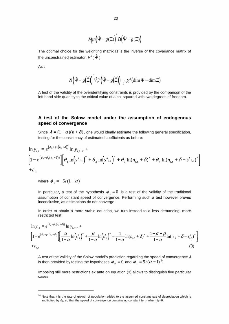
Since λ α δ= − +( )( )1 n , one would ideally estimate the following general specification, testing for the consistency of estimated coefficients as before:
( )( )
( )( )[ ] ( ) ( )[ ]ln ln
ln ln ln( ) ln( )
, ,
,*
,*
,*
, ,*
y e y
e s s n n s
i tn
i t
n ki t
hi t i t i t
hi t
it
it
it
= +
− + + + + + −
+
+ +−
+ +
ϕ ϕ δτ
ϕ ϕ δ θ θ θ δ θ δ
ε
0 1
0 11 1 2 3 4
where ϕ τ α1 5 1= − −( )
In particular, a test of the hypothesis ϕ 1 0= is a test of the validity of the traditional assumption of constant speed of convergence. Performing such a test however proves inconclusive, as estimations do not converge.
In order to obtain a more stable equation, we turn instead to a less demanding, more restricted test:
( )( )
( )( )[ ] ( ) ( )ln ln
ln ln ln( ) ln( )
( )
, ,
,
*
,
*
,*
, ,*
,
y e y
e s s n n s
i tn
i t
ni tk
i th
i t i t i th
i t
it
it
= +
−−
+−
−−
+ + − −−
+ −
+
+ +−
+ +
ϕ ϕ δτ
ϕ ϕ δ αα
βα α
δ α βα
δ
ε
0 1
0 111 1
11
11
3
A test of the validity of the Solow model’s prediction regarding the speed of convergence λ is then provided by testing the hypotheses ϕ 0 0= and ϕ τ α1 5 1= −( ) 24.
Imposing still more restrictions ex ante on equation (3) allows to distinguish five particular cases:
24 Note that it is the rate of growth of population added to the assumed constant rate of depreciation which is
multiplied by ϕ1, so that the speed of convergence contains no constant term when ϕ0=0.
21
A. original equation (3)
B. equation (3) with the restriction ϕ 0 0=
C. equation (3) with the restriction ϕ 1 0=
D. equation (3) with the restriction ϕ τ α1 5 1= −( )
E. equation (3) with the restrictions ϕ 0 0= and ϕ τ α1 5 1= −( ) (pure theoretical model).
Specifications B to E correspond to linear restrictions imposed on the coefficients of equation (3). They are therefore special cases of specification A.
One way of testing the validity of these restrictions consists in estimating specification A, and using ALS to check the consistency of estimated coefficients with the constraints imposed by specifications B to E. As for the case of constant speed of convergence, this is a test carried out ex post on estimated coefficients.
An alternative approach is to estimate all specifications A to E separately, using the same set of instruments, and use Sargan differences to test the restrictions imposed on the coefficients of the explanatory variables given this set of moment conditions: if the restrictions are valid, then the difference between the Sargan statistics computed from the restricted and unrestricted models follows a χ2 with a number of degrees of freedom equal to the increase in the excess of moment conditions over the number of estimated parameters.

22

23
Results
Under the constant speed of convergence hypothesis: the Solow model is not rejected We estimate equation (2’’) as explained in 2.225. Table 1 sums up the results obtained26 for various specifications.
For equations in levels, the set of instruments is made of the lagged values of all first differenced explanatory variables - except sh
27- from t-1 down to t-2. We instrument the first differenced equation by the lagged values of the same explanatory variables in levels from t-2 down to t-3. Both specifications are minimal in that they strike a compromise between estimation accuracy and economy of instruments (see Appendix for a discussion).
Table 128 - Conditional convergence (Standard errors in parentheses)
OLS on levels (τ =2)
First differences instrumented by
lagged levels (τ =1)
Levels instrumented by
lagged first differences
(τ =1)
Levels instrumented by
lagged first differences
(τ =2) Constant
0.04
(0.37) 0.05
(0.01) -0.00 (0.21)
2.41 (0.44)
Ln(Y-τ) 0.93
(0.02) 0.82
(0.07) 0.93
(0.03) 0.65
(0.05)
Ln(n+ δ) -0.14 (0.13)
-0.07 (0.13)
-0.23 (0.07)
-0.40 (0.15)
Ln(sk) 0.16 (0.03)
0.07 (0.05)
0.10 (0.02)
0.16 (0.06)
Ln(sh) 0.01 (0.02)
-0.04 (0.02)
0.02 (0.01)
0.13 (0.04)
Ln(n+δ-sh) -0.01 (0.05)
0.02 (0.03)
0.05 (0.03)
0.20 (0.07)
Sargan (pvalue, df) 34.4
(0.06, 23) 36.4
(0.31, 33) 31.6
(0.07, 21)
OLS estimates are known to be trivially biased since the lagged endogenous variable includes the individual effect. One then expects the coefficient on lagged GDP to be biased upwards. Our results confirm this conjecture: the coefficient given by OLS is 0.93, to be compared with a value of 0.65 given by the GMM estimator for the same τ =2.
The choice of τ =2 for the first differenced model implies a severe loss in terms of number of time series observations. Besides, considering the low amount of autocorrelation on GDP growth rates, there is no need to extend the estimation period to ten years. Consequently, we only test the first differenced model under the assumption τ =1.
Standards errors are large, and few coefficients appear to be significantly different from zero.
25 We use the Summers Heston dataset. Small countries whose population is less than a million, as well as oil
producing countries are excluded from the sample. We end up with 78 countries after eliminating further countries for which human capital variables are not available.
26 We use the program DPD98 written in Gauss for our linear GMM estimations (Arellano and Bond[1998]). 27 Lagged values of lnsh are not included in the set of instruments because its compatibility with the rest of the
instruments is rejected by difference Sargan tests. However, the same test leads to a strong acceptation of ln(n+d-sh) as an instrument.
28 All GMM estimates displayed in this table are second step estimates. See Appendix for a discussion. Steady states variables are defined as the value corresponding to the middle of each convergence sub period.
24
GDP in level exhibits a strong time persistence for τ =1, pointing to a slow convergence towards steady state. The significance of the population growth rate and the saving rate appears to be good in both specifications. This is not the case however for the human capital variables, which turn out to be a lot more significant for the specification τ =2. Indeed, it makes sense to consider that human capital investment does not have a sizeable impact on GDP until roughly a decade. Note that neither our data nor our model allow for a possible heterogeneity in the efficiency of the schooling systems.
These considerations lead us to retain the specification τ =2 for the equation written in levels.
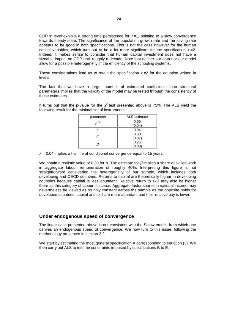
The fact that we have a larger number of estimated coefficients than structural parameters implies that the validity of the model may be tested through the consistency of these estimates.
It turns out that the p-value for the χ2 test presented above is 75%. The ALS yield the following result for the minimal set of instruments:
parameter ALS estimate
e-10λ 0.66 (0.04)
λ 0.04
α 0.30 (0.07)
β 0.26 (0.03)
λ = 0.04 implies a half life of conditional convergence equal to 15 years.
We obtain a realistic value of 0.30 for α. The estimate for β implies a share of skilled work in aggregate labour remuneration of roughly 40%. Interpreting this figure is not straightforward considering the heterogeneity of our sample, which includes both developing and OECD countries. Returns to capital are theoretically higher in developing countries because capital is less abundant. Relative return to skill may also be higher there as this category of labour is scarce. Aggregate factor shares in national income may nevertheless be viewed as roughly constant across the sample as the opposite holds for developed countries: capital and skill are more abundant and their relative pay is lower.
Under endogenous speed of convergence The linear case presented above is not consistent with the Solow model, from which one derives an endogenous speed of convergence. We now turn to this issue, following the methodology presented in section 3.2.
We start by estimating the most general specification A corresponding to equation (3). We then carry out ALS to test the constraints imposed by specifications B to E.

25
Table 2 - Tests ex post of the theoretical constraints based on the unrestricted specification (Standard errors in parentheses)
A
(Benchmark) B
ϕ 0 0= C
ϕ 1 0= D
ϕ α1 10 1= −( )
E ϕ 0 0=
ϕ α1 10 1= −( )
α 0.31 (0.06)
0.33 (0.06)
0.26 (0.05)
0.41 (0.04)
0.40 (0.04)
β 0.26 (0.08)
0.18 (0.07)
0.37 (0.06)
0.12 (0.06)
0.11 (0.06)
ϕ0 -0.32 (0.15)
-0.51 (0.11)
-0.11 (0.12)
ϕ1 -2.68
(-1.32) -4.50 (1.02)
χ² DF
P-value
15.46 28
0.97
4.80 1
0.03
4.14 1
0.04
6.65 1
0.01
7.41 2
0.02
ALS lead to the rejection of all constraints, in particular of the one based on a constant speed of convergence (B), as well as the pure Solow theoretical model (E). It seems from these results that the Solow model is rejected by the data when it is taken seriously, that is when all the theoretical restrictions it imposes are taken into account. Note however that this conclusion may be due to the choice of the reference specification on which ALS are performed. Recall that specification A is not the most general, as explained in section 3.2. The choice made is therefore arbitrary, and gives a particular role to specification A.
We therefore turn to the alternative method based on Sargan differences. Restrictions are now imposed ex ante and tests are carried out on the corresponding estimations. Table 3 presents the results.
Table 3 - Tests based on the estimation of restricted specifications (Standard errors in parentheses)
A
(Benchmark) B
ϕ 0 0= C
ϕ 1 0= D
ϕ α1 10 1= −( )
E ϕ 0 0=
ϕ α1 10 1= −( )
α 0.31 (0.06)
0.40 (0.05)
0.28 (0.06)
0.38 (0.05)
0.40 (0.04)
β 0.26 (0.08)
0.25 (0.05)
0.35 (0.07)
0.18 (0.07)
0.19 (0.04)
ϕ0 -0.32 (0.15)
-0.55 (0.10)
-0.19 (0.14)
ϕ1 -2.68
(-1.32) -3.86 (0.89)
Sargan Sargan based
on W.M.(E) DF
P-value
15.46 22.92
28
0.97
28.55 23.51
29
0.49
18.75
29 0.93
14.5 24.41
29
0.99
25.96 25.96
30
0.68
These specifications can be distinguished by the constraint they impose on ϕ0 and ϕ1. In each case, estimates of α and β are significant and consistent with each other given standard errors.
The estimates of ϕ1 obtained from specification (A) and (B) are consistent with the values computed from the corresponding estimates of α and the theoretical relationship ϕ α1 10 1= −( ) .

26
The Sargan difference tests validate the restrictions that specification (D) imposes on (A) and (E) on (B). One problem in implementing this test is due to the fact that the difference of Sargan statistics are negative. We deal with this by carrying out the test on Sargan statistics obtained by using the same second step weighting matrix. Conclusions are unchanged.
Turning to tests of the restriction ϕ 0 0= :
The difference tests based on Sargan statistics obtained by using the same second step weighting matrix (that of specification (E)) do not reject the restriction ϕ 0 0= . Note however that the difference tests obtained by using different weighting matrices (second step matrices obtained from respectively specifications (D) and (E)) do not confirm this result. While using a unique weighting matrix seems to us to more relevant, one has to admit that contrary to the previous case, conclusions are not robust to a change in the way the test is carried out. They must as a result be considered as fragile.
Despite the robustness of the estimates for α and β across the specifications, and despite the validation of the constraint ϕ α1 10 1= −( ) , the fragile validation of ϕ 0 0= does not allow to conclude sharply in favour of the Solow model.
This is all the more obvious considering the results given by the first method presented above. Whether this fragility points to an insufficient number of observations or must be interpreted as a sign of the weakness of the Solow model as such may not be concluded from this study.
27
Conclusion
Two main conclusions may be drawn from this paper.
First, the estimations carried out under the assumption of constant speed of convergence show that the estimation strategy we suggest, based on the estimation of the model in levels instrumented by lagged first differences, is both more rigorous than MRW’s and more efficient than CEL’s. It is true that these results were obtained at the cost of an additional identifying assumption, that of constant correlation between regressors and the individual effect (stationarity assumption). We do not believe this assumption to be strong. We are comforted in this by the fact that Sargan tests do not reject the consistency of the orthogonality conditions generated by this specification. Asymptotic least squares applied to our linear GMM estimator confirms both the robustness of our estimates and the compatibility of the constraints imposed on them by the theoretical model. Besides, the estimated value for GDP elasticity to physical capital is close to 0.30, a value generally deemed to be realistic.
Secondly, this methodological improvement is not sufficient in itself to provide a validation of the Solow model for two reasons.
To begin with, one may not claim to carry out a rigorous test of a model by estimating an equation obtained by imposing a restriction not derived from the model itself. From this point of view, assuming a constant speed of convergence across countries is theoretically inconsistent. It turns out that our tests carried out under the more general assumption of endogenous speed of convergence do not validate the restriction that the speed of convergence is constant: even if the constant term included in λ appears to be significant, so is the endogenous one. The assumption of constant λ must therefore be viewed at best as a poor approximation only weakly supported by the data.
Given this, tests of the rigorous model where the expression of λ is derived from the Solow model itself, show that the theoretically consistent convergence equation is not fully consistent with the data either. Note however that the estimates of the elasticities of output to physical and human capital are hardly affected, compared to the more restricted case of constant λ.
These results obviously lead to question the adequation of our theoretical framework with the data. This may point either to a misspecification of the production function, to the existence of strong heterogeneity across countries or to the inadequation of the Solow framework altogether. Further research is obviously needed to draw a clear conclusion on the implications in terms of test of the Solow model.

28
29
References
ARELLANO Manuel, BOND Stephen, « Some Tests of Specification for Panel Data: Monte Carlo Evidence and an application to Employment Equations », Review of Economic Studies, 58, 1991
ARELLANO Manuel, BOND Stephen, « Dynamic Panel Data Estimation Using DPD98 for Gauss: A Guide for Users », 1998
ARELLANO Manuel, BOVER Olympia, « Another Look at the Instrumental Variable Estimation of Error-Components Models », Journal of Econometrics, 68, 1995
BARRO Robert, LEE Jong-Wha, « International Comparisons of Educational Attainment », Journal of Monetary Economics, 32, 1993
BLUNDELL Richard, BOND Stephen, « Initial Conditions and moment restrictions in Dynamic Panel Data Models », Journal of Econometrics, 87, 1998
CASELLI Francesco, ESQUIVEL Gerardo, LEFORT Fernando, « Reopening the Convergence Debate: A New Look at Cross-Country Growth Empirics », Journal of Economic Growth, 1:3, 1996
ISLAM, Nazrul, « Growth Empirics: A Panel Data Approach », Quarterly Journal of Economics, 110, 1995
KNIGHT Malcolm, LOAYZA Norman, VILLANEUVA Delano, « Testing the Neoclassical Growth Model », IMF Staff Papers, 40, 1993
MANKIW Gregory, ROMER David, WEIL David, « A Contribution to the Empirics of Economic Growth », Quarterly Journal of Economics, 107:2, 1992
QUAH Dany T., « Empirics for growth and distribution: stratification, polarization and convergence clubs », Journal of Economic Growth, 1997
SOLOW Robert, « A Contribution to the Theory of Economic Growth », Quarterly Journal of Economics, 70, 1956
SUMMERS Robert, HESTON Alan, « A new set of International Comparisons of Real Product and Price Levels Estimates for 130 Countries », Review of Income and Wealth, 34, 1988
TEMPLE Jonathan, « The New Growth Evidence », Journal of Economic Literature, 37, 1999

30
31
Appendix
Solving the model The production function is written:
Y t A t K t H t L t( ) ( ) ( ) ( ) ( )= − −α β α β1
Labour (which equals population by assumption) and technical change (Hicks neutral) are supposed to grow at exogeneous and constant rates n and g:
( ) ( )( ) ( )
N t N e
A t A e
nt
gt
=
=
0
0
( ) ( ) ( )N t H t L t= +
Values per unit of labour (or population i.e. per head) are defined as:
y YN
k KN
h HN
l LN
= = = =
Hence, rewriting the production function:
y t A t k t h t l t( ) ( ) ( ) ( ) ( )= − −α β α β1
Accumulation equations, and steady state The physical capital accumulation equation may be written:
K s Y Kk K= −δ
( )k s y n kk K= − +δ
Human capital accumulation is given by:
( )H s H L Hh H= + −δ
( )h s n hh H= − +δ
The dynamics of unskilled labour accumulation is then obtained from the relation l h+ =1 :
l h= −
In order to define a limit trajectory, we make assumptions on the growth rates of per head variables when this steady state is reached. We assume that the ratio of output to the stock of physical capital is fairly constant over time, therefore that the rates of growth of per head output and per head capital must be identical at steady state. We do not
32
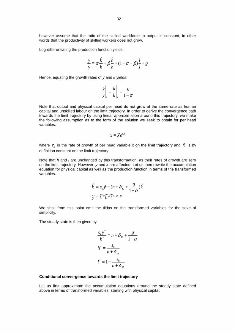
however assume that the ratio of the skilled workforce to output is constant, in other words that the productivity of skilled workers does not grow.
Log-differentiating the production function yields:
( )y
ykk
hh
ll
g= + + − − +α β α β1
Hence, equating the growth rates of y and k yields:
* *
yy
kk
g= =−1 α
Note that output and physical capital per head do not grow at the same rate as human capital and unskilled labour on the limit trajectory. In order to derive the convergence path towards the limit trajectory by using linear approximation around this trajectory, we make the following assumption as to the form of the solution we seek to obtain for per head variables:
x xer tx= ~
where rx is the rate of growth of per head variable x on the limit trajectory and ~x is by definition constant on the limit trajectory.
Note that h and l are unchanged by this transformation, as their rates of growth are zero on the limit trajectory. However, y and k are affected. Let us then rewrite the accumulation equation for physical capital as well as the production function in terms of the transformed variables.
~ ~ ( ) ~
~ ~ ~ ~k s y n g k
y k h l
k K= − + +−
= − −
δα
α β α β
11
We shall from this point omit the tildas on the transformed variables for the sake of simplicity.
The steady state is then given by:
s yk
n g
h sn
l sn
kK
h
H
h
H
*
*
*
*
= + +−
=+
= −+
δα
δ
δ
1
1
Conditional convergence towards the limit trajectory
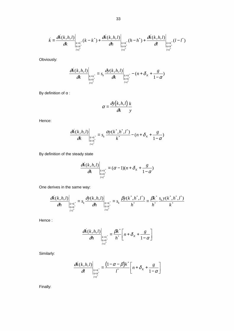
Let us first approximate the accumulation equations around the steady state defined above in terms of transformed variables, starting with physical capital:
33
( , , ) ( )
( , , ) ( )( , , ) ( )*
*
*
*
*
*
*
*
*
* * *k k k h lk
k k k k h lh
h h k k h ll
l lk kh hl l
k kh hl l
k kh hl l
= − + − + −===
===
===
∂∂
∂∂
∂∂
Obviously:
∂∂
∂∂
δα
( , , ) ( , , ) ( )*
*
*
*
*
*
k k h lk
s y k h lk
n gk kh hl l
k k kh hl l
K===
===
= − + +−1
By definition of α :
( )α∂
∂=
y k h lk
ky
, ,
Hence:
∂∂
α δα
( , , ) ( , , ) ( )*
*
*
* * *
*
k k h lk
s y k h lk
n gk kh hl l
k K===
= − + +−1
By definition of the steady state
∂∂
α δα
( , , ) ( )( )*
*
*
k k h lk
n gk kh hl l
K===
= − + +−
11
One derives in the same way:
∂∂
∂∂
β β( , , ) ( , , ) ( , , ) ( , , )*
*
*
*
*
*
* * *
*
*
*
* * *
*
k k h lh
s y k h lh
s y k h lh
kh
s y k h lkk k
h hl l
k k kh hl l
kk
===
===
= = =
Hence :
∂∂
β δα
( , , )*
*
*
*
*
k k h lh
kh
n gk kh hl l
K===
= + +−
1
Similarly:
( )∂∂
α βδ
α( , , )
*
*
*
*
*
k k h ll
kl
n gk kh hl l
K===
=− −
+ +−
1
1
Finally:

34
( )
( )( )( )( )
( ) ( )( ) ( ) ( )
**
**
*
**
*
*
k n g k k kh
h hk
ll l
h n h hl n l l
K
H
H
= + +−
− − + − +− −
−
= − + −= − + −
δα
α β α β
δδ
11
1
Making the first order approximation at the vicinity of the steady state:
y y k k h h l l= = = =* * * *, , ,
Plugging the previous approximations of the dynamics of factor accumulation into the log-differentiated per head production function yields:
( )
( )
( ) ( )
( ) ( )
*
*
*
*
*
*
*
*
*
*
yy
n g k kk
h hh
l ll
n h hh
n l ll
K
H H
= + +−
− − + − + − − −
− + −
− + − − −
α δα
α β α β
δ β δ α β
11 1
1
In order to factorize the analogous expression obtained from the traditional augmented Solow model, the previous literature on convergence (for instance MRW) assumes that depreciation rates on physical and human capital are identical. For the same reason, we have to make the assumption that the rates of depreciation are identical modulo the limit trajectory common rate of growth of output per head and physical capital per head:
δ δα
δH Kg= +−
=1
This restriction is obviously arbitrary. Note however that the rates of depreciation involved are unknown and that the previous condition is by no means more restrictive than the one imposed by MRW. Indeed, this alone does not provide a justification. The assumption is obviously made for convenience as it allows to obtain a simple representation of the dynamics of transformed output. The latter must consequently be viewed as a simplification of the « true » convergence path.
The previous expression may then be factorized into:
( ) ( )( )
*
*
*
*
*
*
yy
n k kk
h hh
l ll
= + − − + − + − − −
δ α α β α β1 1
Since one may also write around the steady state:
( )y yy
k kk
h hh
l ll
− = − + − + − − −*
*
*
*
*
*
*
*α β α β1
Factorising the latter expression into the former yields:
( )( )*
*
yy
n y yy
= + − −δ α 1
Or alternatively:

35
( )( )
d ydt
y y
n
ln (ln ln )*= −
= − +
λ
λ α δ1
Solving the differential equation and writing the limit conditions:
[ ]d y ydt
y y
yy
Ce
C y y
t
ln ln(ln ln )
ln
ln ln
**
*
*
−= − −
=
= −
−
λ
λ
0
The solution is therefore given by:
( )ln ln ln *y e y e yt t= + −− −λ λ0 1
Recall that the above equation has been derived using the concept of transformed output (i.e. such that the rate of growth on the limit trajectory is zero). We seek however to estimate a convergence equation involving the initial measurable per head variables. Obviously, the previous equation is unchanged when expressed in terms of per head variables.
Estimating the previous equation requires that the expression of the steady state is explicited. By definition (in per head variables):
( )( )
( )
( ) ( )δδδ
δδ
βαβα
+−−+=
+−=
+−=
+−+=
+−−++=
nsnn
sl
nshnsyk
Alhky
hh
h
k
lnln1lnln
lnlnln
lnlnlnlnlnln1lnlnln
*
*
**
*****
Hence, returning to per unit of efficient labour values:
( ) ( )ln ln ln ln ln*y s s n s nk h h=−
+−
+ − −−
+ − −−
+αα
βα
α βα
δα
δ1 1
11
11
Hence:
( ) ( )( ) ( ) ( ) ( )
ln ln ln ln
ln ln
y e y e s e s
e n s e n
t tk
th
th
t
= + −−
+ −−
+ − − −−
+ − − −−
+
− − −
− −
λ λ λ
λ λ
αα
βα
α βα
δα
δ
0 11
11
1 11
1 11
The terms appearing in this equation and involving either the level or the rate of growth of technology (i.e. g or A) are unobserved and included in the residual.
By definition of y:
36
ln ln ln ln lny YN
A YN
A gttt
tt
t
t
= − = − −0
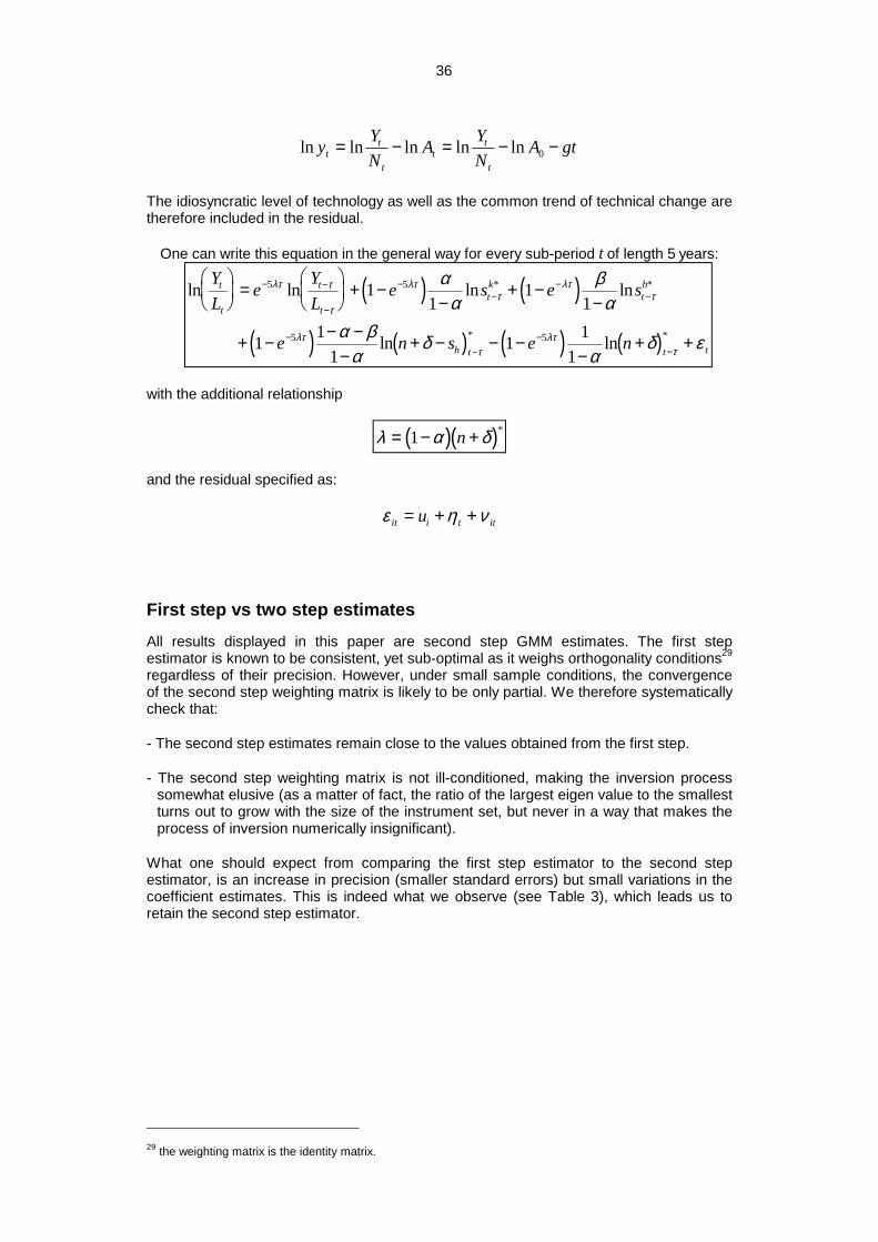
The idiosyncratic level of technology as well as the common trend of technical change are therefore included in the residual.
One can write this equation in the general way for every sub-period t of length 5 years:
( ) ( )
( ) ( ) ( ) ( )
ln ln ln ln
ln ln
* *
* *
YL
eYL
e s e s
e n s e n
t
t
t
ttk
th
h t t t
=
+ −
−+ −
−
+ − − −−
+ − − −−
+ +
− −
−
−−
−−
−−
−−
5 5
5 5
11
11
1 11
1 11
λτ τ
τ
λττ
λττ
λττ
λττ
αα
βα
α βα
δα
δ ε
with the additional relationship
( )( )λ α δ= − +1 n *
and the residual specified as:
ε η νit i t itu= + +
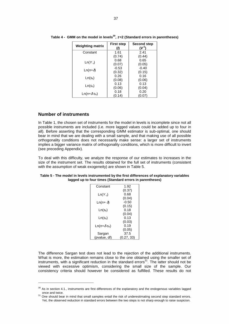
First step vs two step estimates All results displayed in this paper are second step GMM estimates. The first step estimator is known to be consistent, yet sub-optimal as it weighs orthogonality conditions29 regardless of their precision. However, under small sample conditions, the convergence of the second step weighting matrix is likely to be only partial. We therefore systematically check that:
- The second step estimates remain close to the values obtained from the first step.
- The second step weighting matrix is not ill-conditioned, making the inversion process somewhat elusive (as a matter of fact, the ratio of the largest eigen value to the smallest turns out to grow with the size of the instrument set, but never in a way that makes the process of inversion numerically insignificant).
What one should expect from comparing the first step estimator to the second step estimator, is an increase in precision (smaller standard errors) but small variations in the coefficient estimates. This is indeed what we observe (see Table 3), which leads us to retain the second step estimator.
29 the weighting matrix is the identity matrix.
37
Table 4 - GMM on the model in levels30, ττττ =2 (Standard errors in parentheses)
Weighting matrix First step (I)
Second step (V-1)
Constant
1.61 (0.74)
2.41 (0.44)
Ln(Y-τ) 0.68
(0.07) 0.65
(0.05)
Ln(n+δ) -0.53 (0.32)
-0.40 (0.15)
Ln(sk) 0.26 (0.08)
0.16 (0.06)
Ln(sh) 0.13 (0.06)
0.13 (0.04)
Ln(n+δ-sh) 0.18
(0.14) 0.20
(0.07)
Number of instruments In Table 1, the chosen set of instruments for the model in levels is incomplete since not all possible instruments are included (i.e. more lagged values could be added up to four in all). Before asserting that the corresponding GMM estimator is sub-optimal, one should bear in mind that we are dealing with a small sample, and that making use of all possible orthogonality conditions does not necessarily make sense: a larger set of instruments implies a bigger variance matrix of orthogonality conditions, which is more difficult to invert (see preceding Appendix).
To deal with this difficulty, we analyze the response of our estimates to increases in the size of the instrument set. The results obtained for the full set of instruments (consistent with the assumption of weak exogeneity) are shown in Table 5.
Table 5 - The model in levels instrumented by the first differences of explanatory variables lagged up to four times (Standard errors in parentheses)
Constant 1.92 (0.37)
Ln(Y-τ) 0.68 (0.04)
Ln(n+ δ) -0.50 (0.15)
Ln(sk) 0.18 (0.04)
Ln(sh) 0.13 (0.03)
Ln(n+δ-sh) 0.19 (0.05)
Sargan (pvalue, df)
37.5 (0.27, 33)
The difference Sargan test does not lead to the rejection of the additional instruments. What is more, the estimation remains close to the one obtained using the smaller set of instruments, with a significant reduction in the standard errors31. The latter should not be viewed with excessive optimism, considering the small size of the sample. Our consistency criteria should however be considered as fulfilled. These results do not
30 As in section 4.1., instruments are first differences of the explanatory and the endogenous variables lagged
once and twice. 31 One should bear in mind that small samples entail the risk of underestimating second step standard errors.
Yet, the observed reduction in standard errors between the two steps is not sharp enough to raise suspicion.

38
invalidate the use of all instruments compatible with the hypothesis of weak exogeneity, but they do not rest on it.