G Model ARTICLE IN PRESS - cs.purdue.edu · Iyera,∗, Haim Avronb, Georgios Kolliasc, Yves Ineichend, Christopher Carothersa, Petros ... Rensselaer Polytechnic Institute, 110 8th

J

Ao

CPa

b

c

d

a

ARAA

KRHD

1

daarrt

x

Ss[ciwfa

c

AR

h1

ARTICLE IN PRESSG ModelOCS-547; No. of Pages 11

Journal of Computational Science xxx (2016) xxx–xxx

Contents lists available at ScienceDirect

Journal of Computational Science

journa l h om epage: www.elsev ier .com/ locate / jocs

randomized least squares solver for terabyte-sized denseverdetermined systems�

hander Iyera,∗, Haim Avronb, Georgios Kolliasc, Yves Ineichend, Christopher Carothersa,etros Drineasa

Department of Computer Science, Rensselaer Polytechnic Institute, 110 8th Street, Troy, NY, USADepartment of Applied Mathematics, Tel Aviv University, P.O. Box 39040, Tel Aviv, IsraelIBM Research – T.J. Watson Research Center, Yorktown Heights, NY, USAIBM Research – Zurich Research Lab, Zurich, Switzerland

r t i c l e i n f o

rticle history:eceived 28 May 2016ccepted 21 September 2016

a b s t r a c t

We present a fast randomized least-squares solver for distributed-memory platforms. Our solver is basedon the Blendenpik algorithm, but employs multiple random projection schemes to construct a sketch of

vailable online xxx

eywords:andomized numerical linear algebraigh-performance computing

the input matrix. These random projection sketching schemes, and in particular the use of the randomizedDiscrete Cosine Transform, enable our algorithm to scale the distributed memory vanilla implementationof Blendenpik to terabyte-sized matrices and provide up to ×7.5 speedup over a state-of-the-art scal-able least-squares solver based on the classic QR algorithm. Experimental evaluations on terabyte scalematrices demonstrate excellent speedups on up to 16,384 cores on a Blue Gene/Q supercomputer.

ense least squares regression

. Introduction

The explosive growth of data over the past 20 years in variousomains, ranging from physics and biological sciences to economicsnd social sciences, has led to a need to perform efficient and scal-ble analysis on such massive datasets. One of the most widely andoutinely used primitives in statistical data analysis is least-squaresegression: given a matrix A ∈ R

m×n and a vector b ∈ Rm, we seek

o compute

∗ = arg minx ∈ Rn

∥∥Ax − b∥∥

2. (1)

everal algorithms have been proposed to solve large-scale least-quares problems in various distributed and parallel environments1], returning solutions whose accuracy is close to machine pre-ision. Recent approaches for large-scale least-squares problemsnclude communication-avoiding factorizations [2], which scale

ell for a variety of shared memory and distributed memory plat-orms [3] and are based on the classic QR decomposition algorithm,

Please cite this article in press as: C. Iyer, et al., A randomized least sqComput. Sci. (2016), http://dx.doi.org/10.1016/j.jocs.2016.09.007

n O(mn2) algorithm (assuming m ≥ n).Recent years have witnessed an explosion of research on so-

alled Randomized Numerical Linear Algebra [4] (or RandNLA for

� This work was partially supported by the XDATA program of the Defensedvanced Research Projects Agency (DARPA), administered through Air Forceesearch Laboratory contract FA8750- 12-C-0323, as well as by NSF IIS-1302231.∗ Corresponding author.

ttp://dx.doi.org/10.1016/j.jocs.2016.09.007877-7503/© 2016 Elsevier B.V. All rights reserved.

© 2016 Elsevier B.V. All rights reserved.

short) algorithms, which leverage the power of randomization inorder to perform standard matrix computations. One of the coreproblems that have been extensively researched in this emergingfield is the least-squares regression problem of Eq. (1). Sarlos [5]and Drineas et al. [6] introduced the first randomized algorithmsfor this problem. These algorithms are based on the application ofthe sub-sampled Randomized Hadamard Transform to the columnsof the input matrix in order to create a least-squares problem ofsmaller size that can be then solved exactly and whose solutionprovably approximates the solution of the original problem withvery high probability. This was followed by the work of Rokhlinand Tygert [7], who used a subsampled Randomized Fourier Trans-form to form a preconditioner and then used a standard iterativesolver to solve the preconditioned problem. At the same time,Avron et al. [8] introduced Blendenpik, an algorithm and a softwarepackage which was the first practical implementation of a RandNLAdense least-squares solver that consistently and comprehensivelyoutperformed state-of-the-art implementations of the traditionalQR-based O(mn2) algorithms. Since then, there has been extensiveresearch on RandNLA algorithms for regression problems; see Yanget al. [9] for a recent survey.

So far, most research on randomized least-squares regressionalgorithms has focused on the single processor setting, with two

uares solver for terabyte-sized dense overdetermined systems, J.

important exceptions. Meng et al. [10] introduced LSRN, a dis-tributed memory algorithm for least-squares problems based onrandom Gaussian projections. While the algorithm is still an O(mn2)algorithm, the benefits of randomization are apparent with respect

dx.doi.org/10.1016/j.jocs.2016.09.007

dx.doi.org/10.1016/j.jocs.2016.09.007

http://www.sciencedirect.com/science/journal/18777503

http://www.elsevier.com/locate/jocs

dx.doi.org/10.1016/j.jocs.2016.09.007

ING ModelJ

2 tation

tisft

rBptspliAa8Pt1tbocc[u

tddadCtttsa

mlnttwatd

db

l�ro

2s

o

ARTICLEOCS-547; No. of Pages 11

C. Iyer et al. / Journal of Compu

o both constants in the asymptotic analysis, as well as its muchmproved efficiency on parallel environments. Yang et al. [9] con-ider RandNLA in a MapReduce-like framework called Spark. Thisramework is less appropriate for supercomputers, as it is fails toake advantage of their hardware architecture.

In this work, we explore the behavior of Blendenpik-type algo-ithms in a distributed memory setting. We show that variants oflendenpik that use various batchwise transformations to computereconditioners lead to implementations that are not only fasterhan state-of-the-art implementations of baseline least-squaresolvers, but are also able to scale to much larger matrix sizes. Inarticular, we show that a Blendenpik based algorithm can solve

east-squares regression problems with terabyte-sized (and larger)nput matrices. Our implementation and experiments were run onMOS,1 the high-performance Blue Gene/Q supercomputer systemt Rensselaer. AMOS has five racks, 5120 nodes (81,920 cores), and1,920 GB of main memory. AMOS has a peak performance of oneetaFLOP (1015 floating point operations per second), and a 5-Dorus network with 2 GB/s of bandwidth per link and 512 GB/s to

TB/s of bisection network bandwidth per rack, depending on theorus network configuration. Due to runtime constraints imposedy the scheduling system for each partition of AMOS, we limitedur experiments to partitions containing up to 1024 nodes (16,384ores). The Blue Gene/Q architecture supports a hybrid communi-ation framework that uses the MPI (Message Passing Interface)10] standard for distributed communication and multithreadingsing OpenMP [12].

Our main contributions in this paper are: (i) implementa-ion of and experimentation with the Blendenpik algorithm onistributed-memory platforms; (ii) implementation of four ran-omized sketching transforms in the context of the Blendenpiklgorithm; (iii) a batchwise transformation scheme that scales aistributed vanilla implementation of the Randomized Discreteosine Transform in the context of the Blendenpik algorithm by upo three times in terms of matrix sizes, and provides a speedup of upo 7.5 times over a state-of-the-art scalable least-squares solver forera-scale matrices; (iv) a detailed evaluation of four randomizedketching transforms in the context of the Blendenpik algorithmnd their parameters on the BG/Q, using up to 16,384 cores.

The full source code of our batchwise Blendenpik imple-entation is available for download at https://github.com/cjiyer/

ibskylark/tree/batchwiseblendenpik. The rest of this paper is orga-ized as follows. Section 2 describes the Blendenpik algorithm andhe various stages of the algorithm in detail. Section 3 highlightshe distributed Blendenpik implementation in the Blue Gene/Q, asell as scalability issues in our implementation, and describes an

pproach to overcome them. Section 4 first describes experimentso tune our Blue Gene/Q environment for our evaluations and theniscusses the outcome of our experimental evaluations.

Notation. Let A, B, . . . denote matrices and let x, y, z, . . .enote column vectors. Given a vector x ∈ R

m, let ‖x‖22 =∑m

i=1x2i

e (the square of) its Euclidean norm; given a matrix A ∈ Rm×n,

et∥∥A

∥∥2

F=

∑m,ni,j=1A2

ij be (the square of) its Frobenius norm. Let

1 ≥ �1 ≥ �2 · · · ≥ �r > 0 be the nonzero singular values of A, where = rank (A) is the rank of the matrix A. Then, the condition numberf A is equal to �(A) = �1/�r.

. The Blendenpik Algorithm for dense overdeterminedystems


Blendenpik (see Algorithm 1) is a least-squares solver for dense,verdetermined, full column rank least-squares problems that

1 https://secure.cci.rpi.edu/wiki/index.php/Blue Gene/Q.

PRESSal Science xxx (2016) xxx–xxx

computes an approximate solution to the problem of Eq. (1), witha high degree of precision. Given a dense, tall-and-thin matrixA ∈ R

m×n and a column vector b ∈ Rm, the algorithm returns an

approximate solution by executing the following three steps:

1. A preconditioner is constructed by applying a randomized uni-tary (or approximately unitary) transform F to the input matrix Aand then sampling a small number of rows from the transformedmatrix FA to form the matrix Ms.

2. A QR factorization of the sampled matrix Ms is computed, retur-ning an orthogonal matrix Qs and an upper triangular matrix Rs.The latter matrix Rs is then used as a preconditioner for the inputmatrix A.

3. LSQR (an iterative method for solving least-squares problems)is then used to solve a least-squares problem using the precon-ditioned matrix to compute an approximate solution x̂ to theoriginal problem of Eq. (1).

The algorithm uses a simple approach to estimate the conditionnumber of the matrix Rs. This procedure is described in [8] andamounts to computing the product

∥∥Rs

∥∥1

∥∥R−1s

∥∥1, where

∥∥X∥∥

1is

the 1-norm of the matrix X. If that estimate of the condition numberis too small (and thus its inverse is too large), the algorithm tries toconstruct a new preconditioner. If no good preconditioner is con-structed after three repetitions, the algorithm employs a standardsolver to exactly compute the solution. We will use �machine todenote the target machine precision, which in our setting is equalto 2 × 10−15.

Algorithm 1. The Blendenpik algorithm [8].1: Input: A ∈ R

m×n matrix, m � n, rank (A) = n, b ∈ Rm ,

random transform matrixF ∈ Rm×m ,

oversampling factor� ≥ 1, with �n � m.2: Output: approximate solution x̂ to the problem of Eq. (1).3: while TRUE do4: Let S ∈ R

m×m be a random diagonal matrix:

Sii =

{1, withprobability

�n

m

0, otherwise5: Ms = SFA.6: Compute the QR factorization of Ms: Ms = QsRs .7: Let �̂ be an estimate of the condition number of Rs .8: if �̂−1 > 5�machine then

9: y = minz

∥∥AR−1s z − b

∥∥2.

10: Solve Rsx̂ = y and return x̂.11: else if more than three iterations have been performed then12: Solve using the baseline least-squares solver and return.13: end if14: end while

The most important stage of the Blendenpik algorithm is theapplication of the randomized transform F; we will discuss variouschoices for F in Section 2.1. It is worth emphasizing that computingMs as the product SFA in Algorithm 1 is for illustration purposesonly. We will see in Section 2.1 that there are more efficient waysfor computing Ms than simple matrix–matrix multiplication. Theoversampling factor � guarantees that as the number of rows of Ms

will be (in expectation and with high probability) close to �n. Asa result, the computation of the QR decomposition of Ms is com-putationally efficient, since its running time only depends on the“small” dimension n and not on the “large” dimension m. The uppertriangular matrix Rs that is returned by the QR decomposition of Ms

is then used as a preconditioner for the original problem. However,if Rs is ill-conditioned, then we repeat the generation of the ran-


domized transform F in the hope of getting a better-conditionedmatrix Rs. If this procedure fails three times, then an exact solver isemployed to solve the original least-squares problem. We concludethis discussion by stating that while setting � to a smaller value

dx.doi.org/10.1016/j.jocs.2016.09.007

https://github.com/cjiyer/libskylark/tree/batchwiseblendenpik







https://secure.cci.rpi.edu/wiki/index.php/Blue_Gene/Q











IN PRESSG ModelJ

tational Science xxx (2016) xxx–xxx 3

cq

Blfuc

waw

ampo

2

ctfF

vtGwfcmpfrs−wte

F

AfRaromntttaa

oon

Table 1Elemental data distribution overview.

Distribution formatsfor a 2-D process grid

∼[MC , MR] & [MR, MC ][VR, �] & [�, VR][VC , �] & [�, VC ]

[�, �]

MC Matrix column

Distribution orderwithin each griddimension

MR Matrix rowVC Vector in column major orderVR Vector in row major order� Stored on every process

Description[X, Y] Distribute[columns, rows] with

scheme [X, Y][MC , MR] Distribute [columns, rows]

equally among processes



an improve the running time of the QR decomposition of Ms, theuality of the preconditioner typically diminishes as � decreases.

We now briefly discuss the LSQR method that is employed bylendenpik in order to solve the preconditioned least-squares prob-

em. LSQR [13] is an iterative, Krylov-subspace solver that works asollows: given the current iterate xj and the corresponding resid-al error rj = b − Axj, LSQR uses the following criterion to test foronvergence:∥∥∥(

AR−1s

)Trj

∥∥∥2

AR−1s

∥∥rj

∥∥2

≤ �,

here � is a tolerance value that determines the backward errort which the iterative solver terminates. This guarantees a back-ard stable solution to y = min

z

∥∥AR−1s z − b

∥∥2. The residual error

t convergence is used to compute the final backward error esti-ate. The runtime of LSQR is affected by how well-conditioned the

reconditioned system AR−1s is, which in turn is determined by the

versampling factor � .

.1. The randomized transform F

Our work is the first detailed evaluation on a Blue Gene/Q super-omputer of the Blendenpik algorithm with multiple choices forhe randomized transform F. We start by describing a few straight-orward choices for F, as well as more state-of-the-art choices for.

First, F could be a matrix whose entries are independent randomariables, chosen from various well-known distributions. Perhapshe simplest choice is to set the entries of F to be independentaussian random variables of zero mean and variance 1/(�n); weill refer to this construction of F as a Gaussian Random Trans-

orm (GRT). While Meng et al. [10] also use the GRT as theirhoice of randomized transform for the LSRN algorithm, a funda-ental difference between LSRN and Blendenpik is the way the

reconditioner is constructed. The Blendenpik algorithm uses a QRactorization of the sampled matrix Ms whereas the LSRN algo-ithm computes the SVD of Ms to form the preconditioner. A secondtraight-forward choice is to set the entries of F to be +1/

√�n or

1/√

�n with probability 1/2, independently for each entry. Weill refer to this construction as a Random Sign Matrix (RSM). A

hird choice was proposed by Achlioptas in [14] and constructs thentries of F as follows:

ij =

⎧⎨⎩−√

3/(�n), with probability 1/6

0, with probability 2/3

+√

3/(�n), with probability 1/6

gain, all entries are set to their respective values independentlyrom all other entries. We refer to this construction as a Sparseandom Sign Matrix (SRSM). It is worth noting that all threeforementioned constructions, in the context of Blendenpik algo-ithm, would amount to first computing the product SF (essentiallynly constructing the relevant rows of the randomized transformatrix, since rows that correspond to values Sii equal to zero should

ot be constructed) and then applying SF on to A by computinghe product (SF) A. The SRSM transform could take advantage ofhe sparsity of the matrix SF to compute the above product fasterhan the other two transforms. Finally, we conclude by noting thatll three transforms are normalized appropriately in order to bepproximately unitary.


Finally, our last random transform matrix F was proposed in theriginal Blendenpik paper [8]. The construction of F is the productf a random diagonal matrix and a fixed unitary transformation,amely the Discrete Cosine Transform (DCT). In this case, let D be

VC/VR Distribute over processes incolumn/row major wrapping

a random diagonal matrix whose diagonal entries are set to +1or −1 with probability 1/2. Then, let C be the matrix of the Dis-crete Cosine Transform (see [8] for details) and construct F = DC. Wewill refer to this construction of F as the Randomized DCT (RDCT).We note that, in this case, the computation of FA is more efficientthat matrix-matrix multiplication. Indeed, one can apply the DCTmatrix C on the columns of A in a column-wise manner much fasterthan matrix-vector multiplication, by using the properties of theDiscrete Cosine Transform. Then, applying the matrices S and Don the resulting matrix CA is trivial, since they are both diagonalmatrices.

3. Implementing our algorithm on the Blue Gene/Q

The algorithm is implemented on top of the Elemental library[15]. Given a distributed environment over p processes, any densematrix A ∈ R

m×n is partitioned in Elemental into rectangular gridsof sizes r × c in a 2D cyclic distribution, such that p = r × c and bothr and c are O(

√p). Elemental allows a matrix to be distributed in

more than one way. An overview of various data distributions avail-able in Elemental is given in Table 1 (not exhaustive). We use thestandard distribution [MC, MR] listed in Table 1 for dense inputmatrices, in order to exploit operations that are communicationintensive. For column-wise and row-wise vector operations thatrequire local computations to be performed, we use a [�, VC/VR] ora [VC/VR, �] distribution that assigns each column or row vector toa single process. In some cases, we require a matrix or a columnvector to be present across all processes, which is done using the[�, �] format. The notations used henceforth are adapted from Ele-mental for convenience. Ref. [15] gives a comprehensive insighton these notations, describing different data distributions and thecommunication costs involved in redistribution.

We already presented in Section 2.1 various methods of gener-ating the matrix F that is critical in the Blendenpik algorithm. WhenF is a Random Gaussian Transform, or a Random Sign Transform,or a Sparse Random Sign Transform, we generated and applied itwithin Elemental using the standard [MC, MR] data distribution (astraight-forward operation). The only construction of F that meritsadditional discussion is the Randomized Discrete Cosine Transform.In order to apply the RDCT on a matrix A in a column-wise manner,we used the DCT implementation of FFTW [16], a highly opti-mized implementation of the Fast Fourier Transform (FFT), tunedfor underlying architectures that work on multidimensional data.For our purposes, we used the 1-D versions of DCT that operate onElemental’s data distributions. In this case, the [MC, MR] Elemental


distribution is not a suitable format in order to apply FFTW’s DCT,since the data distributed across multiple nodes in a column-wise aswell as in a row-wise manner are locally non-contiguous. However,the implementation in FFTW expects contiguously distributed data

dx.doi.org/10.1016/j.jocs.2016.09.007

ING ModelJ

4 tation

ata[mdi

F

TMruptbdppswt

ttiSatttwbpfoisdVstMMnse

4

tdfet

h



cross the relevant dimensions. We resolve this problem by redis-ributing the data so that all elements of a column or row vectorre owned locally by a process, using either the [VR/VC, *] or the*, VR/VC] distribution of Table 1. In order to apply the DCT, all ele-

ents of a column must be stored locally, i.e., using the [*, VR/VC]istribution. The Elemental pseudocode in order to apply the DCT

n Blendenpik is described in the following steps:

A ⇔

⎧⎪⎨⎪⎩

A[�, VR] = A[MC, MR]

M[�, VR] = F[�, VR]A[�, VR]

M[MC, MR] = M[�, VR]

he A[*, VR] ←− A[MC, MR] redistribution can be thought of as aPI Scatter and an MPI Gather collective pair operation. The cur-ent MPI specifications (MPI 3.0) support sending and/or receivingp to INT MAX (231− 1) elements for any collective operation. Thislaces memory constraints for terascale dense overdetermined sys-ems, as the row sizes increase and more column elements getunched together inside a single process. Hammond et al. [17]emonstrate a library implementation called BigMPI as a wrap-er to current MPI specifications to resolve this problem. However,orting this wrapper to the local MPI implementation of our AMOSupercomputer is a cumbersome task and beyond the scope of ourork. We instead overcame this problem using a batchwise unitary

hat we will discuss next.Recall that the grid distribution of Elemental is cyclic and it

herefore imposes an additional overload during redistribution ofhe input matrices. In more detail, the memory for each processs now shared by more than one columns of the input matrix.ince we are concerned with terascale, over-determined systems,

piecemeal redistribution, where in we select only a few columnso transform at a time is generally preferred. Another limiting fac-or that inhibits Blendenpik performance on terascale matrices ishe communication cost in redistributing matrices after a batch-ise transformation. A straightforward solution is to sample the

atchwise transformed matrix before redistribution to generate thereconditioner. Let a matrix A ∈ R

m×n be distributed in an [MC, MR]ormat and let there be p MPI processes (for sake of this example) inur distributed environment. We divide the matrix A columnwisento b submatrices given by A(1), A(2), . . ., A(b), redistribute eachubmatrix A(i)[�, VR] ← A(i)[MC, MR] : i ∈ {1, . . ., b}, perform ran-om unitary transformations on each submatrix M(i)[�, VR] ← F[�,R]A(i)[�, VR] : i ∈ {1, . . ., b}, sample from each of the transformedubmatrices M(i)

s [�, VR] ← S[�, VR]M(i)[�, VR] : i ∈ {1, . . ., b}, redis-ribute back each of the sampled b submatrices M(i)

s [MC, MR] ←(i)s [�, VR] : i ∈ {1, . . ., b}, and finally merge them all in the Ms[MC,R] matrix. The number of columns in each submatrix and thus the

umber of submatrices b can be tuned depending on the dimen-ions of the matrix and the number of MPI processes p used in ourvaluations.

. Evaluation

To generate terascale-sized dense matrices, we randomly per-urb sparse matrices with values generated from a standard normal


istribution. We relied on the UFL Sparse matrix collection [18]or obtaining matrices of different condition numbers and coher-nce values. We chose to work with the Yoshiyasu Mesh matrix,2

he ESOC Springer matrix,3 and the Rucci4 matrix from the UFL

2 http://www.cise.ufl.edu/research/sparse/matrices/Yoshiyasu/mesh deform.tml.3 http://www.cise.ufl.edu/research/sparse/matrices/Springer/ESOC.html.4 http://www.cise.ufl.edu/research/sparse/matrices/Rucci/Rucci1.html.


Sparse matrix collection for creating our datasets. Table 2 showsthe particular matrices that were used in our evaluations: startingwith the aforementioned three matrices, we first densified them byadding random Gaussian noise as discussed above. Then, we repli-cated and vertically concatenated them (with different noise addedat each replication step) in order to create tall-and-thin matrices.Each matrix in Table 2 is suffixed with the number of replicationsand vertical concatenations of the base dense matrix. For example,to construct Yoshiyasu-24, we started with the Yoshiyasu Meshmatrix, added noise to create 24 slightly different copies of thismatrix, and then vertically concatenated these 24 copies to get atall-and-thin matrix.

We now describe our evaluation metrics. Recall that A ∈ Rm×n

is the input matrix and b ∈ Rm is the target vector. Let x̂ be the

approximate solution returned by Algorithm 1 and let x* be theoptimal solution to the problem of Eq. (1). Let t̂run be the runningtime of Algorithm 1 and let t∗run be the running time of the baselineElemental least-squares solver. Then, our first accuracy metric is therelative error of the approximate solution x̂, given by the followingformula:∥∥Ax̂− Ax∗

∥∥2/∥∥Ax∗

∥∥2. (2)

We also compute the backward error of the approximate solutionas follows:∥∥AT

(b − Ax̂

)∥∥2. (3)

Finally, the speedup of Algorithm 1 is defined as

t∗run/t̂run. (4)

4.1. AMOS environment setup

Our objective in the evaluation section is to provide a thoroughevaluation of Blendenpik-type solvers for terascale least-squaresproblems from three primary viewpoints: scalability, performance,and accuracy. We tuned AMOS to evaluate the Blendenpik imple-mentation against optimum baseline performance and scalability.We selected a combination of the number of OpenMP threads pernode and the number of MPI processes per node that gave maxi-mum performance for the baseline Elemental least-squares solveron AMOS. We measured the average time taken by the baselinesolver over five runs for all possible MPI and OpenMP combinationsfor two dense matrices: a random matrix whose entries were gen-erated uniformly at random in the interval [−1,1] with dimensions1,320,000 × 38,000 and the ESOC-4 matrix (Table 2) with dimen-sions 1,308,248 × 37,830. The AMOS system can execute up to 64MPI processes with one OpenMP thread, or one MPI process with64 OpenMP threads, or any combination of the two that results ina product of MPI processes and OpenMP threads that is equal to64 in a single node. We used a bgclang/LLVM build of the baselineElemental solver for our evaluations.

As seen in Table 3, the performance of the baseline Elemen-tal solver improved as the number of OpenMP threads per nodeincreased for a single MPI process per node. Similarly, the per-formance also increased with increasing MPI processes per nodefor a single OpenMP thread. However, the performance droppedwhen many MPI processes compete for CPU resources with severalOpenMP threads in the system. The maximum performance is real-ized for 32 OpenMP threads for a single MPI process (Table 3), whileit immediately degraded when the number of threads reached 64.One possible reason could be because of possible thread synchro-


nization during floating point operations in the BG/Q CPU cores.The choice of one MPI process and 32 OpenMP threads per BlueGene/Q node was the standard configuration that we selected forour evaluations.

dx.doi.org/10.1016/j.jocs.2016.09.007

http://www.cise.ufl.edu/research/sparse/matrices/Yoshiyasu/mesh_deform.html












http://www.cise.ufl.edu/research/sparse/matrices/Springer/ESOC.html











http://www.cise.ufl.edu/research/sparse/matrices/Rucci/Rucci1.html











ARTICLE IN PRESSG ModelJOCS-547; No. of Pages 11

C. Iyer et al. / Journal of Computational Science xxx (2016) xxx–xxx 5

Table 2Matrices used in our evaluations.

Matrix name # of rows (Millions) # of columns # of entries (Billions) Size (TBs)

Yoshiyasu-1 0.234

9393

2.198 0.016Yoshiyasu-24 5.616 52.756 0.384Yoshiyasu-48 11.233 105.512 0.768Yoshiyasu-72 16.849 158.268 1.152Yoshiyasu-96 22.466 211.025 1.535Yoshiyasu-120 28.082 263.781 1.919Yoshiyasu-144 33.699 316.537 2.303Yoshiyasu-168 39.315 369.294 2.687Yoshiyasu-192 44.932 422.050 3.070

ESOC-1 0.327

37,830

12.373 0.090ESOC-8 2.616 98.982 0.720ESOC-16 5.233 197.964 1.440ESOC-24 7.849 296.946 2.160ESOC-32 10.466 395.928 2.880ESOC-40 13.082 494.910 3.600ESOC-48 15.698 593.892 4.321ESOC-56 18.315 692.874 5.041ESOC-64 20.931 791.856 5.761

Rucci-1 1.978109,900

217.369 1.581Rucci-2 3.956 434.739 3.163Rucci-3 5.933 652.108 4.744

Table 3Runtime analysis to select an optimal hybrid MPI/OpenMP configuration for our scaling experiments. Each run was averaged over five times on 128 BG/Q nodes. All runtimesare in seconds(lower runtimes are preferred); the optimal performance (bold running times) was observed when one MPI process per node and 32 OpenMP threads per nodewere used.

OpenMP threads per node random matrix A, of dimensions 1.32M × 38K; average �(A) = 1.4084 ± 1.1 * 10−4

MPI processes per node

1 2 4 8 16 32 64

1 8734.48 4613.62 2996.67 2187.48 1477.89 1878.74 1755.572 4499.6 2637.91 1762.49 1580.48 1240.34 1826.52 –4 2349.32 1565.67 1156.55 1334.04 1168.86 – –8 1276.73 1097.84 922.341 2261.12 – – –16 800.443 1057.67 1193 – – – –32 628.171 1081.64 – − – – –64 686.517 – – – – – –

OpenMP threads per node ESOC-4 matrix A, of dimensions 1.3082M × 38K; average �(A) = 1.4594 * 106 ± 11.0268

MPI processes per node

1 2 4 8 16 32 64

1 9304.71 5205.42 2737.43 2067.88 1378.84 1809.77 –2 4831.84 2922.68 1640.01 1542.24 1133.12 1741.58 –4 2567.38 1741.82 1091.47 1236.9 1023.93 – –8 1463.21 1207.34 898.165 1219.18 – – –

1.234

4

iG(sbvmei

16 961.26 1026.97 8932 742.075 919.704 –

64 744.563 – –

.2. Runtime environment evaluation

One of the key factors that influence scalability considerationss the performance of the runtime environment of the AMOS Blueene/Q system. The AMOS system supports both standard GNU

4.7.2) as well as LLVM/bgclang5 environments [19]. Fig. 1 demon-trates the speedup for the baseline Elemental least-squares solver,uilt with bgclang, over the baseline solver built with GNU forarious matrices from Table 2 on 512 BG/Q nodes. The baseline Ele-ental solver achieves a significant speedup in the LLVM/bgclang


nvironment due to the highly optimized linear algebraic routinesmplemented in the BG/Q Math libraries, the ESSL (Engineering

5 http://trac.alcf.anl.gov/projects/llvm-bgq.

– – – –– – – –– – – –

Scientific Subroutine Library), and the MASS (Mathematical Accel-eration Subsystem).

To solve the least-squares regression problem, the baseline Ele-mental solver computes the QR decomposition of the input matrix.The QR decomposition is computed via a sequence of matrix mul-tiplications of orthogonal matrices and the input matrix. In thissetting, ESSL outperforms the BLAS routines built with the standardGNU compiler for the Blue Gene/Q system. The speedup for theYoshiyasu matrix is much better than the one achieved for the ESOCSpringer matrix; this is due to the fact that the QR decompositiondepends quadratically on n and linearly on m.

4.3. Evaluating the four randomized transforms


One of the main objectives of this paper is to evaluate theBlendenpik algorithm with respect to the evaluation metrics givenin Eqs. (2)–(4). We aim to understand the performance of the four

dx.doi.org/10.1016/j.jocs.2016.09.007

http://trac.alcf.anl.gov/projects/llvm-bgq








ARTICLE ING ModelJOCS-547; No. of Pages 11

6 C. Iyer et al. / Journal of Computation

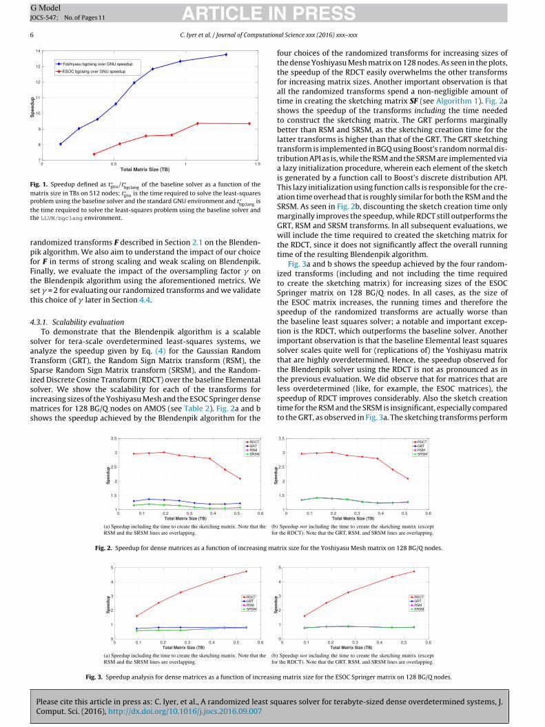
Fig. 1. Speedup defined as t∗gnu/t∗bgclang

of the baseline solver as a function of thematrix size in TBs on 512 nodes; t∗gnu is the time required to solve the least-squaresproblem using the baseline solver and the standard GNU environment and t∗ istt

rpfFtst

4

saTSisims

bgclang

he time required to solve the least-squares problem using the baseline solver andhe LLVM/bgclang environment.

andomized transforms F described in Section 2.1 on the Blenden-ik algorithm. We also aim to understand the impact of our choiceor F in terms of strong scaling and weak scaling on Blendenpik.inally, we evaluate the impact of the oversampling factor � onhe Blendenpik algorithm using the aforementioned metrics. Weet � = 2 for evaluating our randomized transforms and we validatehis choice of � later in Section 4.4.

.3.1. Scalability evaluationTo demonstrate that the Blendenpik algorithm is a scalable

olver for tera-scale overdetermined least-squares systems, wenalyze the speedup given by Eq. (4) for the Gaussian Randomransform (GRT), the Random Sign Matrix transform (RSM), theparse Random Sign Matrix transform (SRSM), and the Random-zed Discrete Cosine Transform (RDCT) over the baseline Elemental


olver. We show the scalability for each of the transforms forncreasing sizes of the Yoshiyasu Mesh and the ESOC Springer dense

atrices for 128 BG/Q nodes on AMOS (see Table 2). Fig. 2a and bhows the speedup achieved by the Blendenpik algorithm for the

Fig. 2. Speedup for dense matrices as a function of increasing ma

Fig. 3. Speedup analysis for dense matrices as a function of increasin


four choices of the randomized transforms for increasing sizes ofthe dense Yoshiyasu Mesh matrix on 128 nodes. As seen in the plots,the speedup of the RDCT easily overwhelms the other transformsfor increasing matrix sizes. Another important observation is thatall the randomized transforms spend a non-negligible amount oftime in creating the sketching matrix SF (see Algorithm 1). Fig. 2ashows the speedup of the transforms including the time neededto construct the sketching matrix. The GRT performs marginallybetter than RSM and SRSM, as the sketching creation time for thelatter transforms is higher than that of the GRT. The GRT sketchingtransform is implemented in BGQ using Boost’s random normal dis-tribution API as is, while the RSM and the SRSM are implemented viaa lazy initialization procedure, wherein each element of the sketchis generated by a function call to Boost’s discrete distribution API.This lazy initialization using function calls is responsible for the cre-ation time overhead that is roughly similar for both the RSM and theSRSM. As seen in Fig. 2b, discounting the sketch creation time onlymarginally improves the speedup, while RDCT still outperforms theGRT, RSM and SRSM transforms. In all subsequent evaluations, wewill include the time required to created the sketching matrix forthe RDCT, since it does not significantly affect the overall runningtime of the resulting Blendenpik algorithm.

Fig. 3a and b shows the speedup achieved by the four random-ized transforms (including and not including the time requiredto create the sketching matrix) for increasing sizes of the ESOCSpringer matrix on 128 BG/Q nodes. In all cases, as the size ofthe ESOC matrix increases, the running times and therefore thespeedup of the randomized transforms are actually worse thanthe baseline least squares solver; a notable and important excep-tion is the RDCT, which outperforms the baseline solver. Anotherimportant observation is that the baseline Elemental least squaressolver scales quite well for (replications of) the Yoshiyasu matrixthat are highly overdetermined. Hence, the speedup observed forthe Blendenpik solver using the RDCT is not as pronounced as inthe previous evaluation. We did observe that for matrices that are


less overdetermined (like, for example, the ESOC matrices), thespeedup of RDCT improves considerably. Also the sketch creationtime for the RSM and the SRSM is insignificant, especially comparedto the GRT, as observed in Fig. 3a. The sketching transforms perform

trix size for the Yoshiyasu Mesh matrix on 128 BG/Q nodes.

g matrix size for the ESOC Springer matrix on 128 BG/Q nodes.

dx.doi.org/10.1016/j.jocs.2016.09.007



Fig. 4. Speedup for dense matrices as a function of increasing matrix size.

ber o

ci

4

aptftcabotsopf

bnnanmswbTco

pfa51s

Fig. 5. Strong scaling as a function of the num

omparably when the time to construct the sketching matrix is notncluded (see Fig. 3b).

.3.2. Scalability evaluation for terascale matricesThe key objective of our work here is to evaluate the Blendenpik

lgorithm as a solver for terascale overdetermined least-squaresroblems. As seen in Section 4.3.1, using the RDCT transform inhe Blendenpik algorithm outperforms the other randomized trans-orms even for moderately sized matrices. Hence, we only evaluatehe scalability of Blendenpik using the RDCT for terascale matri-es. Fig. 4a and b shows the scalability of our solver on 512 nodesnd 1024 nodes respectively on AMOS. As discussed earlier, thease Elemental least-squares solver scales quite well for highlyverdetermined dense matrices. Hence the speedup observed forhe Blendenpik solver compared to the baseline solver is not asignificant as seen in Fig. 4a. However, for matrices that are lessverdetermined, the runtime and thus the speedup of the Blenden-ik algorithm improves considerably. This observation is obviousor the ESOC Springer matrix, shown in Fig. 4b.

One observation that is particularly significant is the effect ofatchwise RDCT on the speedup as the matrix size increases. Theumber of columns transformed in a single batch depends on theumber of rows of the matrix as well as on the minimum spacevailable across all processes to allocate the columns. Thus, as theumber of rows increases, fewer and fewer columns fit in a batchaking the batchwise transformation step slower. This is the rea-

on underlying the observation that the speedup peaks at the pointhere the entire transformed matrix is able to fit into memory and

eyond this stage, the batchwise processing slowdown kicks in.his effect is more pronounced for an increasing number of repli-ations of the ESOC Springer matrix and the Rucci matrix in Fig. 4bn 1024 BG/Q nodes.

In general, the Blendenpik algorithm scales excellently as com-ared to the baseline Elemental solver. While the baseline solverails to execute for the Yoshiyasu-192 (see Table 2) on 512 nodes,


s well as for the ESOC-36 (ESOC matrix with 36 replications) in12 nodes and the ESOC-68 (ESOC matrix with 68 replications) in024 nodes, the Blendenpik solver is able to scale to such matrixizes. Another important aspect of the Blendenpik algorithm for

f Blue Gene/Q nodes used in our evaluation.

the terascale matrices from Table 2 is that the steps 11–12 is neverperformed as the densification step of constructing these matri-ces generates moderately well-conditioned matrices, and hence thepreconditioner constructed is also well-conditioned.

4.3.3. Performance evaluationWe also evaluate the strong and weak scaling performance of

the Blendenpik algorithm as a function of the (increasing) numberof the Blue Gene/Q nodes. Fig. 5a and b shows the strong scalingperformance of the four randomized sketching transforms on theYoshiyasu-4 matrix (i.e., the base Yoshiyasu Mesh matrix replicatedfour times), as well as on the base ESOC Springer dense matrix,respectively. We observe that the speedup of the Blendenpik solverincreases marginally with an increasing number of BG/Q nodes;this effect is more pronounced in the case of the Yoshiyasu Meshmatrix rather than the ESOC Springer matrix. However, this advan-tage is offset as the baseline Elemental solver performs comparablyto the batchwise Blendenpik solver for 512 BG/Q nodes. This slow-down in the batchwise Blendenpik solver is mainly because of theQR preconditioning phase that does not scale as well as the ran-domized sketching matrices and the LSQR stages of the Blendenpikalgorithm, as the number of BG/Q nodes increases. The RDCT out-performs the other sketching transforms by at least a factor of twofor all BG/Q node configurations.

Finally, the weak scaling performance of the Blendenpik algo-rithm on the Yoshiyasu Mesh and ESOC Springer matrices for thefour randomized sketching transforms that we evaluate in thiswork is shown in Fig. 6a and b, respectively. We observe that theruntime for the RDCT on the Yoshiyasu Mesh matrix increases sub-linearly as the matrix size increases and as the number of BG/Qnodes increases; at the same time, there is a significant bump in therunning time of the baseline solver. Also, the runtimes for the otherrandomized sketching transforms (GRT, RSM, and SRSM) remainapproximately constant as the matrix size and the number of BG/Qnodes both increase. Furthermore, the runtimes for the random-


ized sketching transforms are much better than the runtime of thebaseline solver. Interestingly, the runtime of the RDCT for the ESOCmatrix keeps diminishing, even as the number of rows and thenumber of BG/Q nodes keeps increasing. As we already discussed in

dx.doi.org/10.1016/j.jocs.2016.09.007


8 C. Iyer et al. / Journal of Computational Science xxx (2016) xxx–xxx

trix s

tiwstoBtram

4

aT(BraOgpoFsWfsiiowcti

4

uatstobipbfidtb

Fig. 6. Weak scaling as a function of ma

he strong scaling analysis, the primary bottleneck for the reductionn performance as the number of BG/Q nodes increases has to do

ith the runtime of the QR decomposition at the preconditioningtage. However, the size of the sampled matrix, which is the input tohe QR decomposition at the preconditioning stage, is independentf the number of rows of the original input matrix. As additionalG/Q nodes are allocated, the performance of the QR decomposi-ion at the preconditioning stage improves. This boosts the overalluntime of the Blendenpik algorithm, an effect that is observed forll four randomized sketching transforms, even though it is muchore pronounced for the RDCT.

.3.4. Numerical stability evaluationWe evaluate the numerical stability of the Blendenpik solver for

ll randomized sketching transforms as the matrix size increases.he numerical stability is captured by the relative error (see Eq.2)) and the backward error (see Eq. (3)). Our evaluations on 128G/Q nodes show a relative error within 11-12 digits of accu-acy for all randomized sketching transforms for both the ESOCnd Yoshiyasu matrices. Thus, these values are much better than(√

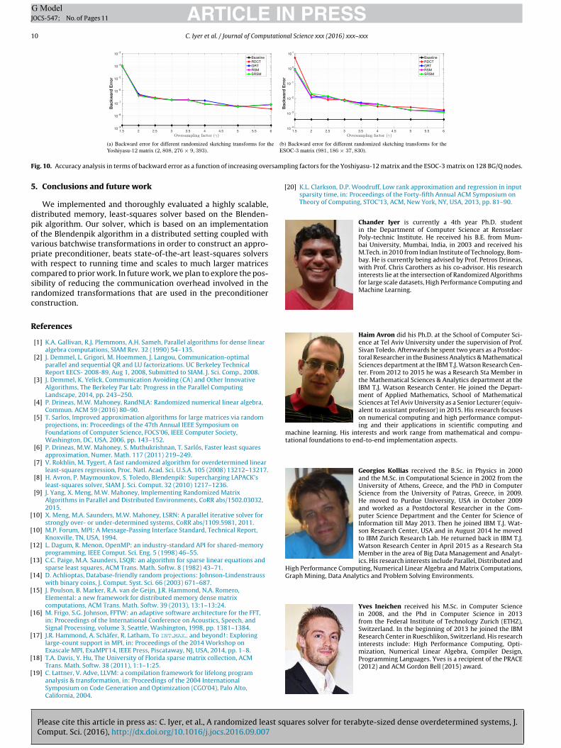
�machine), which is well within the bounds on the relative erroruarantees given by Drineas et al. [6]. We skip the relative errorlots in the interest of space and describe the numerical stabilityf the Blendenpik solver captured by the backward error instead.ig. 7a and b captures the behavior of the backward error as theize of the Yoshiyasu Mesh and ESOC Springer matrices increases.

e observe that the backward error for all randomized trans-orms is roughly two orders of magnitude worse than the baselineolver. Furthermore, the backward error for all transforms, includ-ng the baseline solver for the ill-conditioned ESOC Springer matrix,s several orders of magnitude worse (approximately five ordersf magnitude worse) than the backward error for the relativelyell-conditioned Yoshiyasu Mesh matrix. While the relative error

aptures the stability of the solution, the backward error captureshe stability of the system, and the more ill-conditioned the systems, the worse the error will be.

.3.5. Numerical stability evaluation for terascale matricesWe evaluate the numerical stability for the Blendenpik solver

sing the relative error metric of Eq. (2) for increasing matrix sizesnd for 512 Blue Gene/Q nodes, for both the Yoshiyasu Mesh andhe ESOC matrices; see Fig. 8a. We only show results for the RDCT,ince all four randomized sketching transforms have approximatelyhe same behavior for both the relative and the backward error. Webserve that the relative error is again well within the O(

√�machine)

ounds. The numerical stability defined by backward error is shownn Fig. 8b for both the baseline Elemental solver and the Blenden-ik solver. We observe that the ESOC Springer matrix has worseackward error than the Yoshiyasu Mesh matrix (approximately


ve orders of magnitude worse) for increasing matrix sizes; this isue to its high condition number. However, the backward error ofhe Blendenpik solver is comparable to the backward error of theaseline solver. This error could potentially be improved by either

izes and number of Blue Gene/Q nodes.

using more than one preprocessing stages or by selecting largersample sizes for the preconditioning stage. The latter choice wouldlead to worse running times and reduced speedups as the size ofthe input matrices increases. Another approach to overcome thistradeoff is to apply a random sketching transform matrix F as pro-posed in the ground-breaking paper of Clarkson and Woodruff [20]and then apply the RDCT to FA. We refer the reader to [20] for adetailed description of their original construction and simply notethat applying the resulting matrix SF on the input matrix A takestime proportional to the sparsity of the input matrix A.

4.4. The effect of the oversampling factor �

An important choice in the construction of an efficient precon-ditioner in the context of the Blendenpik algorithm is the value ofthe oversampling factor � that decides the number of rows (equal,in expectation, to �n) of the preconditioner. Of particular interestis an analysis of the behavior of the various randomized sketch-ing transforms in the Blendenpik solver with respect to the metricsdescribed in Section 4 as a function of � . We evaluate the Blenden-pik solver on the Yoshiyasu-12 and the ESOC-4 matrices on 128BG/Q nodes as a function of � , where � ranges between 1.5 and sixin increments of 0.5. We seek to understand the effect of � on thescalability and the numerical stability of the Blendenpik algorithm.

Fig. 9a and b shows the speedup of the Blendenpik algorithmfor increasing values of the oversampling factor � for the vari-ous randomized sketching transforms on the Yoshiyasu-12 and theESOC-4 matrices, respectively. Fig. 9a reveals several interestingobservations as the oversampling factor � increases. The speedupof the RDCT increases marginally as the value of � increases. This isbecause the computational cost of applying the RDCT dominates theQR preconditioning and the LSQR stages for highly overdeterminedmatrices. As the oversampling factor increases, the transformationtime remains the same, while the computational time of the QRdecomposition, which is comparatively much smaller, increases.Furthermore, as the oversampling factor � increases, a better pre-conditioner is constructed, which leads to a faster convergence timefor LSQR. However, the speedups of the other randomized sketch-ing transforms decrease, mainly due to the dominant cost of thetime that it takes to apply the random sketching transformation asthe oversampling factor � increases.

Fig. 9b shows the monotonically decreasing speedup of the RDCTas the oversampling factor � increases for the ESOC-3 matrix. Thisis due to the computational cost of the QR preconditioning stage,which dominates the computational time needed to apply the ran-domized sketching matrix as well as the LSQR solver stage, since theinput matrix is not as overdetermined as the Yoshiyasu-12 matrix.As the oversampling factor � increases, the time to compute the QR


decomposition in the preconditioning stage also increases, lead-ing to an overall reduced speedup. This behavior is also exhibitedby the other randomized sketching transforms. Furthermore, thespeedup of the RDCT easily overwhelms the speedup of the other

dx.doi.org/10.1016/j.jocs.2016.09.007



Fig. 7. Numerical stability (backward error analysis) as a function of (increasing) matrix sizes for the Yoshiyasu Mesh and the ESOC Springer matrices for 128 BG/Q nodes.

oshiy

rs

iefoo

fEeitkAac

4

wCf

Fig. 8. Numerical stability as a function of matrix size for the Y

andomized sketching transforms for increasing values of the over-ampling factor � .

As discussed in Section 4.3.4, the numerical stability is measuredn terms of relative and backward error. Also, again as discussedarlier, the relative error for all randomized sketching transformsor both the ESOC and the Yoshiyasu matrices is within 11-12 digitsf accuracy, and hence we measure the numerical stability in termsf the backward error only.

Fig. 10a and b shows the behavior of the backward error as aunction of the oversampling factor � for the Yoshiyasu-12 and theSOC-3 matrix, respectively. It is worth noting that the backwardrror for both matrices sharply decreases for all randomized sketch-ng transforms at � = 2 and monotonically continues to decrease ashe oversampling factor � increases. Thus, � equal to two acts as anee point validating our choice for � for our tera-scale evaluations.ll the randomized sketching transforms exhibit errors that arepproximately within the same order of magnitude for the varioushoices of the oversampling factor � .

.5. Summarizing our empirical evaluations


To help the reader parse our extensive empirical evaluations,e briefly summarize our findings. (i) The Randomized Discreteosine Transform (RDCT) outperforms the Gaussian Random Trans-orm (GRT), the Random Sign Matrix Transform (RSM) and the

Fig. 9. Speedup as a function of the (increasing) oversampling factor � for

asu Mesh and the ESOC Springer matrices on 512 BG/Q nodes.

Sparse Random Sign Matrix Transform (SRSM) in terms of scal-ability and performance. (ii) The computational cost of the variousstages of the Blendenpik solver is determined by how overdeter-mined the input matrix is. The more overdetermined the matrix, thehigher the computational cost of the random sketching transformstage. As the matrix becomes less overdetermined, the runningtime of the QR decomposition in the preconditioning stage becomesmore and more dominant. This is especially true for the RDCT.(iii) The scalability of the batchwise Blendenpik implementationis determined by the number of columns in each batch of theRDCT transform, which in turn is determined by the number ofrows of the matrix. As the number of rows increases, the run-time of the batchwise sketching transform stage worsens, leadingto reduced speedups. (iv) The batchwise Blendenpik solver usingthe RDCT demonstrates significant strong and weak scaling forall matrices. (v) The Blendenpik solver demonstrates excellentnumerical stability in terms of the forward error for increasingmatrix sizes. The backward error is somewhat worse yet compa-rable to the backward error achieved by the baseline Elementalsolver. (vi) The oversampling factor � determines the quality ofthe preconditioner for the Blendenpik solver. Choosing a higher


oversampling factor leads to better numerical stability. However,higher oversampling factors lead to a reduced performance. Thistradeoff becomes less significant as the input matrix becomes moreoverdetermined.

the Yoshiyasu-12 matrix and the ESOC-3 matrix on 128 BG/Q nodes.

dx.doi.org/10.1016/j.jocs.2016.09.007


10 C. Iyer et al. / Journal of Computational Science xxx (2016) xxx–xxx

F rsamp

5

dpovpwcsrc

R

[

[

[

[

[

[

[

[

[

[

[

Research Center in Rueschlikon, Switzerland. His researchinterests include: High Performance Computing, Opti-mization, Numerical Linear Algebra, Compiler Design,Programming Languages. Yves is a recipient of the PRACE

ig. 10. Accuracy analysis in terms of backward error as a function of increasing ove

. Conclusions and future work

We implemented and thoroughly evaluated a highly scalable,istributed memory, least-squares solver based on the Blenden-ik algorithm. Our solver, which is based on an implementationf the Blendenpik algorithm in a distributed setting coupled witharious batchwise transformations in order to construct an appro-riate preconditioner, beats state-of-the-art least-squares solversith respect to running time and scales to much larger matrices

ompared to prior work. In future work, we plan to explore the pos-ibility of reducing the communication overhead involved in theandomized transformations that are used in the preconditioneronstruction.

eferences

[1] K.A. Gallivan, R.J. Plemmons, A.H. Sameh, Parallel algorithms for dense linearalgebra computations, SIAM Rev. 32 (1990) 54–135.

[2] J. Demmel, L. Grigori, M. Hoemmen, J. Langou, Communication-optimalparallel and sequential QR and LU factorizations. UC Berkeley TechnicalReport EECS- 2008-89, Aug 1, 2008, Submitted to SIAM. J. Sci. Comp., 2008.

[3] J. Demmel, K. Yelick, Communication Avoiding (CA) and Other InnovativeAlgorithms, The Berkeley Par Lab: Progress in the Parallel ComputingLandscape, 2014, pp. 243–250.

[4] P. Drineas, M.W. Mahoney, RandNLA: Randomized numerical linear algebra,Commun. ACM 59 (2016) 80–90.

[5] T. Sarlos, Improved approximation algorithms for large matrices via randomprojections, in: Proceedings of the 47th Annual IEEE Symposium onFoundations of Computer Science, FOCS’06, IEEE Computer Society,Washington, DC, USA, 2006, pp. 143–152.

[6] P. Drineas, M.W. Mahoney, S. Muthukrishnan, T. Sarlós, Faster least squaresapproximation, Numer. Math. 117 (2011) 219–249.

[7] V. Rokhlin, M. Tygert, A fast randomized algorithm for overdetermined linearleast-squares regression, Proc. Natl. Acad. Sci. U.S.A. 105 (2008) 13212–13217.

[8] H. Avron, P. Maymounkov, S. Toledo, Blendenpik: Supercharging LAPACK’sleast-squares solver, SIAM J. Sci. Comput. 32 (2010) 1217–1236.

[9] J. Yang, X. Meng, M.W. Mahoney, Implementing Randomized MatrixAlgorithms in Parallel and Distributed Environments, CoRR abs/1502.03032,2015.

10] X. Meng, M.A. Saunders, M.W. Mahoney, LSRN: A parallel iterative solver forstrongly over- or under-determined systems, CoRR abs/1109.5981, 2011.

10] M.P. Forum, MPI: A Message-Passing Interface Standard, Technical Report,Knoxville, TN, USA, 1994.

12] L. Dagum, R. Menon, OpenMP: an industry-standard API for shared-memoryprogramming, IEEE Comput. Sci. Eng. 5 (1998) 46–55.

13] C.C. Paige, M.A. Saunders, LSQR: an algorithm for sparse linear equations andsparse least squares, ACM Trans. Math. Softw. 8 (1982) 43–71.

14] D. Achlioptas, Database-friendly random projections: Johnson-Lindenstrausswith binary coins, J. Comput. Syst. Sci. 66 (2003) 671–687.

15] J. Poulson, B. Marker, R.A. van de Geijn, J.R. Hammond, N.A. Romero,Elemental: a new framework for distributed memory dense matrixcomputations, ACM Trans. Math. Softw. 39 (2013), 13:1–13:24.

16] M. Frigo, S.G. Johnson, FFTW: an adaptive software architecture for the FFT,in: Proceedings of the International Conference on Acoustics, Speech, andSignal Processing, volume 3, Seattle, Washington, 1998, pp. 1381–1384.

17] J.R. Hammond, A. Schäfer, R. Latham, To INT MAX.. and beyond!: Exploringlarge-count support in MPI, in: Proceedings of the 2014 Workshop onExascale MPI, ExaMPI’14, IEEE Press, Piscataway, NJ, USA, 2014, pp. 1–8.

18] T.A. Davis, Y. Hu, The University of Florida sparse matrix collection, ACM


Trans. Math. Softw. 38 (2011), 1:1–1:25.19] C. Lattner, V. Adve, LLVM: a compilation framework for lifelong program

analysis & transformation, in: Proceedings of the 2004 InternationalSymposium on Code Generation and Optimization (CGO’04), Palo Alto,California, 2004.

ling factors for the Yoshiyasu-12 matrix and the ESOC-3 matrix on 128 BG/Q nodes.

20] K.L. Clarkson, D.P. Woodruff, Low rank approximation and regression in inputsparsity time, in: Proceedings of the Forty-fifth Annual ACM Symposium onTheory of Computing, STOC’13, ACM, New York, NY, USA, 2013, pp. 81–90.

Chander Iyer is currently a 4th year Ph.D. studentin the Department of Computer Science at RensselaerPoly-technic Institute. He received his B.E. from Mum-bai University, Mumbai, India, in 2003 and received hisM.Tech. in 2010 from Indian Institute of Technology, Bom-bay. He is currently being advised by Prof. Petros Drineas,with Prof. Chris Carothers as his co-advisor. His researchinterests lie at the intersection of Randomized Algorithmsfor large scale datasets, High Performance Computing andMachine Learning.

Haim Avron did his Ph.D. at the School of Computer Sci-ence at Tel Aviv University under the supervision of Prof.Sivan Toledo. Afterwards he spent two years as a Postdoc-toral Researcher in the Business Analytics & MathematicalSciences department at the IBM T.J. Watson Research Cen-ter. From 2012 to 2015 he was a Research Sta Member inthe Mathematical Sciences & Analytics department at theIBM T.J. Watson Research Center. He joined the Depart-ment of Applied Mathematics, School of MathematicalSciences at Tel Aviv University as a Senior Lecturer (equiv-alent to assistant professor) in 2015. His research focuseson numerical computing and high performance comput-ing and their applications in scientific computing and

machine learning. His interests and work range from mathematical and compu-tational foundations to end-to-end implementation aspects.

Georgios Kollias received the B.Sc. in Physics in 2000and the M.Sc. in Computational Science in 2002 from theUniversity of Athens, Greece, and the PhD in ComputerScience from the University of Patras, Greece, in 2009.He moved to Purdue University, USA in October 2009and worked as a Postdoctoral Researcher in the Com-puter Science Department and the Center for Science ofInformation till May 2013. Then he joined IBM T.J. Wat-son Research Center, USA and in August 2014 he movedto IBM Zurich Research Lab. He returned back in IBM T.J.Watson Research Center in April 2015 as a Research StaMember in the area of Big Data Management and Analyt-ics. His research interests include Parallel, Distributed and

High Performance Computing, Numerical Linear Algebra and Matrix Computations,Graph Mining, Data Analytics and Problem Solving Environments.

Yves Ineichen received his M.Sc. in Computer Sciencein 2008, and the Phd in Computer Science in 2013from the Federal Institute of Technology Zurich (ETHZ),Switzerland. In the beginning of 2013 he joined the IBM


(2012) and ACM Gordon Bell (2015) award.

dx.doi.org/10.1016/j.jocs.2016.09.007

http://refhub.elsevier.com/S1877-7503(16)30150-8/sbref0005














































































































































































































































































































































































































































































































ING ModelJ

tation

AhNL

fIocc8

Foundation (NSF) as a Program Director in the Information and Intelligent Systems(IIS) Division and the Computing and Communication Foundations (CCF) Division(2010–2011). Prof. Drineas has published over 90 articles in conferences and jour-nals in Theoretical Computer Science, Numerical Linear Algebra, and statistical data



Professor Chris Carothers is a faculty member in theComputer Science Department at Rensselaer Polytech-nic Institute. He received the Ph.D., M.S., and B.S. fromGeorgia Institute of Technology in 1997, 1996, and 1991,respectively. Prior to joining RPI in 1998, he was aresearch scientist at the Georgia Institute of Technology.His research interests are focused on massively paral-lel computing which involve the creation of high fidelitymodels of extreme-scale networks and computer sys-tems. These models have executed using nearly 2,000,000processing cores on the largest leadership class supercom-puters in the world. Professor Carothers is an NSF CAREERAward winner as well as Best Paper award winner at the

CM-SIGSIM PADS Conference for 1999, 2003 and 2009. Since joining Rensselaer,e has developed a world-class research portfolio which includes funding from theSF, the U.S. Department of Energy, Army Research Laboratory, Air Force Researchaboratory, as well as several companies, including IBM, General Electric, and AT&T.

Additionally, Professor Carothers serves as the Director for the Rensselaer Centeror Computational Innovations (CCI). CCI is a partnership between Rensselaer and


BM. The center provides computation and storage resources to diverse networkf researchers, faculty, and students from Renssleaer, government laboratories, andompanies across a number of science and engineering disciplines. The agship super-omputer is a 1 petaFLOP IBM Blue Gene/Q system with 80 terabytes of memory,1,920 processing cores and over 2 petabytes of disk storage.

PRESSal Science xxx (2016) xxx–xxx 11

Professor Petros Drineas is an Associate Professor at theComputer Science Department of Rensselaer PolytechnicInstitute. Prof. Drineas earned a PhD in Computer Sciencefrom Yale University in May of 2003, and a BS in ComputerEngineering and Informatics from the University of Patras,Greece, in July of 1997. Prof. Drineas’ research interestslie in the design and analysis of randomized algorithmsfor linear algebraic problems, as well as their applicationsto the analysis of modern, massive datasets. Prof. Drineasreceived an NSF CAREER in 2006; was a Visiting Professorat the US Sandia National Laboratories during the fall of2005; was a Visiting Fellow at the Institute for Pure andApplied Mathematics at the University of California, Los

Angeles in the fall of 2007; and was a Visiting Professor at the University of CaliforniaBerkeley in the fall of 2013. Prof. Drineas has also served the US National Science


analysis.

dx.doi.org/10.1016/j.jocs.2016.09.007

Documents

G Model ARTICLE IN PRESS - cs.purdue.edu · Iyera,∗, Haim Avronb, Georgios Kolliasc, Yves Ineichend, Christopher Carothersa, Petros ... Rensselaer Polytechnic Institute, 110 8th