1

G16.4409 Advanced Magnetic Resonance Imaging

Medical Image Registration – outline of the lecture

Henry Rusinek & Artem Mikheev Multiple images are often acquired at different times, often different modalities. It is desirable to compare images of patient cohorts. ‘Rigid body’ assumption: structures of interest do not deform or distort. Ex: the brain within the skull, the bones. The assessment of registration accuracy is very important. The error propagation is understood for one algorithm − landmark registration. For other approaches, the algorithm usually provide no useful indication of accuracy. Types of images: There is a huge variety of medical images: microscopic images of histological sections, video images, images of the eye taken with a camera, x-ray images. Developments are driven by the desire to make better use of three-dimensional tomographic modalities: CT, MRI, SPECT and PET. These are the easiest modalities from the point of view of image registration because the sampling is uniform along each axis (but not necessarily isotropic).

2

Definitions, notation and terminology

Registration = co-registration = spatial normalization :: alignment of two images (same or different subjects, same or different modalities). The term spatial normalization is usually restricted to intersubject situation. Registration consists of two tasks:

1) Determining a transformation T that relates points in one image (source) with the position of the corresponding points in another image (target).

Task 1) determines a mapping between coordinates. If we wish to overlay the images or to subtract one from another, then we need to do also task 2):

2) Applying the transformation T to the source image.

The coregistered source is only defined in the region of overlap A ∩T(B) The medical images A B are derived from a real object (the patient) and have a limited field of view that does not normally cover the entire patient. The field of view is likely to be different for the two images. This is a very important factor, which accounts for a good deal of the difficulty in devising accurate and reliable registration algorithms. Due to the discrete nature of medical images, interpolation is necessary for any realistic transformation.

Example of two tasks: 1) Determining the spatial mapping T : T = -12.3, -9.2, 3.8, 0.016, -1.676, -0.107, 1.452, 1.452, 1.421 2) Applying T to the source image -- T(B). Nowt we can compare signal, overlay, subtract, etc. T is not an intensity mapping: it does not make source image look like the target.

3

4

Registration algorithms that make use of geometrical features in the images such as points, lines and surfaces, determine the transformation T by identifying features such as sets of image points that correspond to the same physical entity visible in both images, and calculating T for these features. In one approach to registration, called the method of moments, a part of the body is first delineated from images A and B using a segmentation algorithm, giving the binary volumes A’ and B’. The images are then registered by first aligning the centroids (from the first-order moment) of A’ and B’, and then aligning the principal axes of A’ and B’ (from the second-order moment). Registration algorithms that are based on image intensity values work differently. They iteratively determine the image transformation T that optimizes a similarity measure. These algorithms tend to be iterative, they make successive adjustments to T and keep checking if the algorithm has converged. For registration algorithms that make use of corresponding geometrical features, the difference in field of view of images A and B can cause difficulties, as features identified in one image may not be present in the second. The dependence of field of view tends to be less important for registration algorithms that make use of image intensity values to iteratively determine T.

The discrete nature of the images

An important property of medical images is that they are discrete. They sample the object at a finite number of voxels. In general, this sampling is different for source and target images. Also, the sampling is commonly anisotropic, that is it varies with direction in the image.

5

Problems: * interpolation algorithms are imperfect – blurring/ringing

The intersection of the discrete domains A and T (B) is likely to be the empty set, because no sample points will exactly overlap. It is necessary to interpolate between sample positions and to take account of the difference in sample spacing.

* be careful when the source B has higher resolution than target A. In this case, we risk aliasing when we resample from B to A - we should first blur B before resampling.

Types of transformation

For most current applications of medical image registration, both A and B are three dimensional, so T transforms from 3D space to 3D space. Most medical image registration algorithms additionally assume that the transformation is rigid body with six degrees of freedom: three translations and three rotations. The key characteristic -- all distances are preserved. We can also allow for anisotropic scaling and sheering (skews). A transformation that includes translations, rotations, scaling and skews is referred to as affine. Afine transformation preserves parallel lines.

6

Rigid vs affine vs deformable

Scanner introduced errors that can result in scaling or skew terms, and affine tr. are often used to overcome these problems. In neuroscience we may wish to align images from different subjects using affine tr. For most organs in the body, many more degrees of freedom are necessary to describe the tissue deformation. Even in the brain (child development, lesion growth) affine tr. may be inadequate -- more than 12 degrees of freedom may be needed.

Linear transformation?

We often say linear for affine, but this is mathematically incorrect. In mathematics, a linear function is a map f: x→y between two vector spaces that preserves vector addition and scalar multiplication. The linear functions can be expressed as y=Mx, M = matrix, x,y = vectors.

The translational part of an affine transformation is not linear. An affine map is more correctly described as the composition of linear transformations with translations. Reflections are linear transformations, but they are undesirable in medical image registration -- it might result in a patient having a surgery on the wrong side of her body! Affine transformations should not include reflections.

7

Representation of affine transformation

Homogeneous coordinates system

Ordinary vector algebra uses matrix multiplication to represent linear transformations, and vector addition to represent translations. Using a trick of homogeneous coordinates it is possible to represent both using matrix multiplication. The trick requires a move to 4th dimension. All vectors are augmented with a "1" at the end, and all matrices are augmented with an extra row of zeros at the bottom, an extra column — the translation vector — to the right, and a "1" in the lower right corner.

⎥⎥⎥⎥

⎦

⎤

⎢⎢⎢⎢

⎣

⎡

⎥⎥⎥⎥

⎦

⎤

⎢⎢⎢⎢

⎣

⎡

=

⎥⎥⎥⎥

⎦

⎤

⎢⎢⎢⎢

⎣

⎡

11000333231232221131211

1'''

zyx

tzaaatyaaatxaaa

zyx

Linear transformation (matrix) always maps the origin to the origin. Since vectors with 1 in the last entry doesn’t approach the origin, translations within this subset using linear transformations are possible. Using homogeneous coordinates we can combine any number of affine transformations into one by multiplying the matrices. This is used extensively by graphics software.

8

9

One-to-one transformations

Since the same object (patient) is imaged with the same or different modalities, it would at first seem that the desired transformation T should be one-to-one (bijective). This means that each location in the source image B gets transformed to a single point in the target image A and vice versa. There are several situations in which this does not happen. * dimensionality of A, B is different (registration of a 2D x-ray to a 3D CT scan

* differences in image field of view

* sampling differences

* registration of images from different subjects

* subject before and after surgery

10

Registration may correct image distortions

Skew distortion common in CT – undesirable gantry tilt may rotate the image plane with respect to the axis of the bed. The gantry tilt angle may not unknown, so the skew could be represented in the registration transformation. PET and SPECT distortions caused by misalignment of the detector heads or uncertainty in the centre of rotation -- halo artefacts MR images distortions: * miscalibrated gradients cause voxel dimensions to be incorrect, and a scaling error will be present in the data. (This can be corrected using phantom measurements). * If the static magnetic field B0 is not uniform over the subject, then the field gradients will distort expected linear variation in resonant frequency with position. (B0 inhomogeneity dependens on the object being imaged -- local susceptibility changes.) * since above distortion depends on the field inhomogeneity as a proportion of the imaging gradient strength, it can be reduced by increasing the gradient strength * patient motion during CT or MR imaging -- currently an unsolved problem that makes registration of such datasets very difficult * ghost artifacts - different registration transformation needed for each ghost?

Rigid body registration using points (landmarks)

Points or landmarks are the most widely image features used in registration. (Other features are surfaces and crest lines). Point-based registration: * Identify and label corresponding points The corresponding points are called homologous landmarks -- they should represent the same feature in the different images. * compute transformation T from these points * apply T to the image

11

Procrustes* problem

Given two lists of non-coplanar points P = P1, P2, … ,Pn and Q = Q1, Q2, … ,Qn, find the transformation T which minimizes || T(P) - Q ||. P, Q are the n x 3 matrices, T(P) is the corresponding matrix of transformed points, || . . . || is a matrix norm, the simplest being the Frobenius norm:

2/12

⎟⎟⎠

⎞⎜⎜⎝

⎛= ∑∑

i jijij aa

The case of rigid body and affine transformation have known solutions: Golub G. H. and van Loan C. F. Matrix Computations. Johns Hopkins University Press, Baltimore, MD, 1996.

Dryden I and Mardia K. Statistical Shape Analysis. Wiley, New York, 1998.

Fitzpatrick J et al. Predicting error in rigid-body, point-based registration. IEEE Trans Medical Imaging 17, 694–702, 1998.

* in Greek mythology, a villainous son of Poseidon who forced travelers to fit into his bed by stretching their bodies or cutting off their legs

12

Solution of the classical (rigid body) Procrustes problem

1. Replace points P and Q by shifting the coordinate system to their centroids p0, q0. Pi’ = Pi – p0, Qi’ = Qi – p0

(This reduces the problem to the orthogonal Procrustes problem in which T is a rotation) 2. Construct the 3-by-3 matrix A := (P’)t Q’ 3. Perform the singular value decomposition* A = UDVt

4. a) The rotation part of the solution is R = VUt (verify determinant = +1, not -1) 4, b) translation part of the solution is t = q0 – R p0, see a tutorial on SVD by Dr. Sonia Leach: [SVD_tutorial.pdf]

13

Surface matching: the head-and-hat algorithm

Pelizzari et al proposed a surface matching technique that became known as the ‘head-and-hat’ algorithm. Two equivalent surfaces are identified in the images:

• the first surface (the head) is represented as a stack of discs

• the second surface is a list of unconnected 3D points. The registration transformation is determined by iterative optimization, transforming the hat surface with respect to the head surface, until the closest fit of the hat onto the head is found. The measure of goodness of fit is the average distance between a point on the hat and the nearest point on the head, in the direction of the centroid of the head. The method can be prone to error for convoluted surfaces: the metric used does not always measure the distance between a hat point and the closest point on the head surface -- the nearest head point will not always lie in the direction of the centroid.

Pelizzari CA et al. Accurate three-dimensional registration of CT, PET, and/or MR images of the brain J. Comp Assist Tomogr 13, 20-26, 1989.

14

15

Distance transform

A modification to the head-&-hat algorithm is to use a distance transform to preprocess the head images. A distance transform is applied to raster of voxels: it labels all voxels with their distance from the surface of the object. The cost per iteration is substantially reduced.

Advantages of surface fitting over landmark method:

• the correspondence of individual points is not needed; it is sufficient that the points be on the boundary of the same anatomical structure

• the elimination of the expert observer to identify corresponding points. As usual, there remains a risk of getting stuck in a local minimum.

Tsui W-H and Rusinek. Fast surface-fitting algorithm for 3-D image registration. Medical Imaging: Image Processing, SPIE Vol 1898, 11-20, Sep. 1993.

Rusinek H and Tsui W-H. Principal axes and surface fitting methods for three-dimensional image registration. J Nucl Med 34:2019-2024, 1993.

16

Iterative closest point

The algorithm was originally proposed (Besl & McKay 1992) for the registration of 3D collected data to a model. It has then been applied with success to medical images (Cuchet et al 1995, Maurer et al 1998). The algorithm is designed to work with different representations of surface data: point sets, line segment sets (polylines), curves, triangle sets, and surfaces. For medical image registration the most relevant representations are point\and triangle sets. There are two iterative stages:

• identifying the closest model point for each data point,

• apply rigid body Procrustes solution to find the transformation relating these points sets

The algorithm redetermines the closest point set and continues until it finds the local minimum match between the two surfaces, based on some tolerance threshold. Besl PJ and McKay ND. A method for registration of 3-D shapes. IEEE Trans Pattern Anal Mach Intell 14, 239-256, 1992.

Cuchet E et al. Registration in neurosurgery and neuroradiotherapy applications. J Image Guided Surg 1, 198-207, 1995.

Maurer CR Jr et al. Rgistration of head CT images to physical space using a weighted combination of points and surfaces. IEEE Trans Med Imaging 17, 753-761, 1998.

Registration using crest lines The idea is to use distinctive features on surfaces. Assume that the surfaces are smooth, so that is possible to differentiate up to third order. It is possible to define two principal curvatures k1 and k1, k1>k1, at each point on a surface with associated principal directions. Crest lines are the loci of the surface where the value k1 is locally maximal in its principal direction. Images can be registered by aligning the crest lines.

For medical images with strong edges (bones on CT) the crest lines can be identified directly from the voxel arrays. For other situations (MRI) surface segmentation is first needed. Smoothing is done along with differentiation in order to reduce sensitivity to noise.

Gueziec A and Ayache N. Smoothing and matching of 3-D space curves. Int J Comput Vision 12, 79-104, 1994.

Pennec X and Thirion J-P. A framework for uncertainty and validation of 3-D registration methods based on points and frames. Int J Comput Vision 25, 203-29, 1997

17

Registration using voxel similarity measures

We can calculate the registration transformation T by optimizing a measure derived directly from the voxel values using some voxel similarity measure, rather than from structures such as points or surfaces. We still need iterations to determine T. For such method it is important to distinguish intra-modality from inter-modality registration. Intra-modality: after coregistration and subtraction, we expect to see noise in most places, except for a few regions with some change. If there were a registration error, we would expect to see artefactual structure in the difference image. In this application, voxel similarity measures could be the root mean square difference* (RMSD) or the mean absolute difference. The RMSD measure is widely used for serial MRI registration, including Friston’s statistical parametric mapping (SPM95) software. Hajnal JB et al. A registration and interpolation procedure for subvoxel matching of serially acquired MR images J Comput Assist Tomogr 19, 289-296, 1995.

Friston KJ et al. Spatial registration and normalisation of images. Human Brain Mapping 2, 165-189, 1995.

18

RMSD measure is very sensitive to a small number of voxels that have very large intensity differences between images (contrast studies). The effect of outlier voxels can be reduced by using the mean absolute difference.

Correlation technique

A slightly less strict assumption would be that, at registration, there is a linear relationship between the intensity values in the images. In this case, the optimum similarity measure is the correlation coefficient R or cross correlation:

19

nzz

R BTA∑= )(

)(.)(− ...)( ==

A

AAA Sdevst

SavgSz BTz ,

where S is the signal intensity of a voxel, A denotes the target image, B the source image, T the current estimate of the transform, n the number of voxels in the overlap A∩T(B) . Lemieux L et al.The detection and significance of subtle changes in mixed-signal brain lesions by serial MRI scan matching and spatial normalization. Med Image Anal 2, 227-242, 1998.

Ratio image uniformity

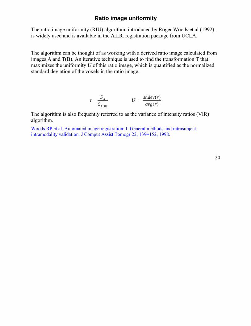
The ratio image uniformity (RIU) algorithm, introduced by Roger Woods et al (1992), is widely used and is available in the A.I.R. registration package from UCLA. The algorithm can be thought of as working with a derived ratio image calculated from images A and T(B). An iterative technique is used to find the transformation T that maximizes the uniformity U of this ratio image, which is quantified as the normalized standard deviation of the voxels in the ratio image.

)()(.

)( ravgrdevstU

SSr

BT

A ==

The algorithm is also frequently referred to as the variance of intensity ratios (VIR) algorithm. Woods RP et al. Automated image registration: I. General methods and intrasubject, intramodality validation. J Comput Assist Tomogr 22, 139=152, 1998.

20

21

Intermodality registration using voxel similarity measures

With intermodality registration, there is no simple relationship between the intensities in the images A and B. 1. It is still possible to create from one modality a new image with intensity characteristics similar to a different modality. For MR–CT registration, we can transform CT so that bone (bright on CT) is re-mapped to very low intensities. In a T1-weighted MRI bone is dark. Transformed CT and MRI can be registered by cross correlation. 2. SPM95 intermodality within-subject PET-MRI registration algorithm*. The signal from PET images comes predominantly from the grey matter, so let’s segment the grey matter in MR, smooth it to spatial resolution of PET, apply cross-correlation, 2. Registration of strong 3D intensity edges: although A and B are very different, they may have quite similar edges. We can apply derivatives to both images A and B to be registered produces two derived images that can be registered by cross correlation.

*Friston KJ et al. Spatial registration and normalisation of images. Human Brain Mapping 2, 165-189, 1995.

22

Partitioned intensity uniformity

The first widely used intermodality registration algorithm that used a voxel similarity measure was due to Roger Woods. This involved a fairly minor change to the source code of their RIU technique, but greatly transformed its functionality. This algorithm makes two assumption: All voxels with a particular MR signal intensity represent the same tissue type. The values of corresponding PET voxels should also be similar to each other. PIU algorithm (for simplicity assume 8-bit signal intensity range):

• partition MRI into 256 separate sparse isointensity volumes: v0,v1,v2,…,v255 based on the value of MRI voxels

• map these subvolumes onto PET space, yielding 256 sparse PET volumes compute uniformity (normalized standard deviation?) within each of 256 PET volumes.. Note: the two modalities are treated differently, depending on which is partitioned. Woods RP et al. MRI-PET registration with automated algorithm. J Comput Assist Tomogr 17, 536-546, 1993.

Information theory – Entropy

An important measure of information in signal and image processing is the Shannon–Wiener entropy

pp log−

ii

i ppH log∑−= H measures the information supplied by a finite set of events whose probabilities are given by p1, p2, ... pn. * If all p’s are 1/n, then H is increasing with n * equalizing probabilities increases the entropy * H will have a maximum value if all events have equal probability of occurring and minimum value of zero if the probability of one event is 1 (rest = 0). Image entropy is calculated from the histogram entries.

23

Image entropy is normally calculated from the histogram entries. If all voxels in an image have the same intensity, the histogram contains a single non-zero element with p=1, so H=0. If the image includes some features, the histogram will be equalized, increasing the entropy. Smoothing reduces information content and lowers H.

Consider the difference image. Any misregistration will lead to edge artefacts that increase the entropy. Very similar images can, therefore, be registered by iteratively minimizing the entropy of the difference image.

Buzug TM and Weese J. Image registration for DSA quality enhancement. Computerized Imaging Graphics 22, 103, 1998.

24

Joint entropy

For two images A and B to align, we have two values at each voxel location for any estimate of the transformation T. Joint entropy measures the amount of information we have in the two images combined. The joint entropy H(A,B) has a similar -p log(p) expression as standard entropy, except that p(a,b) is the probability of signals a, b occurring together. For image entropy, we partition the intensity space into 2D ‘bins’. For example, MR and CT head images being registered (see figure) could have 4096 (12 bits) intensity values, leading to a very sparse 2D histogram with 4096 by 4096 elements.

Q: which axis plots MR signal?

Standard image histograms (“marginal” distribution) are obtained by projecting the joint 2D histogram onto x, y axes for A and B. As can be seen, the joint histogram disperses with increasing misregistration. The brightest regions of the 2D histogram gets less bright, and the number of dark regions is reduced. We can register images by minimizing joint entropy.

25

Limitation of joint entropy

In the process of coregistration we iterate T and measure joint entropy of A and T(B). This entropy is very dependent on the overlap Ω between A and T(B). For example, a change in T may alter the amount of air in the overlap. The air region will occupy the lowest value intensity bins near a = 0, b = 0. If T increases the overlap of air, joint entropy will go down. Joint entropy minimization algorithm will therefore seek to maximize the amount of air in the overlap.

26

Mutual information and normalized mutual information

A solution to the overlap problem is to consider the information contributed to the overlapping volume Ω by each image. Mutual information: I(A,B) = H(A)+H(B)-H(A,B) Normalized mutual information: I’(A,B) = [H(A)+H(B)]/H(A,B)

Ai

i

Ai ppAH log)( ∑

Ω∈

−=H(A,B) = joint entropy, )()( log)( BTi

i

BTi ppBH ∑

Ω∈

−= I(A,B) can be also expressed using conditional probabilities. In maximizing mutual information, we seek for solutions that have a low joint entropy together with high marginal entropies. I(A,B) was independently proposed for intermodality medical registration by researchers in Leuven, Belgium, & MIT in USA. Collignon A et al. Automated multi-modality image registration based on information theory. Inf Proc in Med Imaging. Dordrecht: Kluwer Academic, pp 263-274, 1995. Maes F et al. Multimodality image registration by maximization of mutual information. IEEE Trans Med Imaging 16, 187-198, 1997. Viola PA. Alignment by maximization of mutual information. PhD Thesis, Massachusetts Institute of Technology, 1995. Wells WM. Multi-modal volume registration by maximization of mutual information. Med Image Anal 1, 35-51, 1996.

27

Plots of joint entropy and mutual information for vertical misalignments of two MRI head images: PD-weighted and T2-weighted (dual eacho). The misalignment varied between -6 and +6 mm in 0.2 mm increments. Subvoxel translation was achieved using trilinear interpolation.

• mutual information varies more smoothly with misregistration than joint entropy.

• subvoxel interpolation will blur the images, resulting in local extrema in parameter space. (This problem may be reduced by preblurring the data).

28

29

Relationship to partitioned image uniformity

Mutual information can be thought of as a measure of how well one image explains the other, and is maximized at the optimal alignment. Knowing the intensity value a in A, can we predict the intensity value in T(B)? With high mutual information, knowing the value of a voxel in image A should reduce the uncertainty for the value of the corresponding location in image B. This is a generalization of the assumption made by Woods in his PIU measure, which assumes that at registration the uniformity of T(B) corresponding to a given a in A should be minimal. Two structures which have the same intensity in image A (bone and air in MRI) may have different intensities in image B (bone and air in CT). If we have a low-intensity voxel in imageA=MRI, then at correct alignment we know that this should either be air or bone in the CT. The histogram of CT intensity values corresponding to low intensities in MR will have two sharp peaks -> low entropy. Even though the MR intensity is a pretty good predictor of the CT intensity, PIU would not work well, giving high variability of CT signal.

Thank you!