Embed Size (px)
Citation preview
International Institute for Applied Systems AnalysisSchlossplatz 1 • A‐2361 Laxenburg • Austria
Telephone: (+43 2236) 807 • Fax: (+43 2236) 71313E‐mail: [email protected] • Internet: www.iiasa.ac.at
GAINS Online: Tutorial for advanced users
GAINS Development Team ([email protected])
Version 1.0, October 2009

Page | 2

Page | 3
Preface
IIASA's Atmospheric Pollution and Economic Development (APD) Program carries out applied interdisciplinary research in order to develop innovative modeling tools that identify strategies to protect the local, regional, and global atmosphere while imposing the least burden on economic development. This research brings together the geo‐physical and economic aspects of pollution control within one assessment framework. Together with a network of collaborators, APD uses this framework as a basis for conducting practical policy analysis in different regions of the world.
The guide serves the purpose of providing an insight on how to derive and update data in the GAINS model. The terminology used here enables the guide to be used by everybody, without special analytical skills or advanced knowledge in environmental and social sciences.
We recommend this guide especially for researchers, policy‐makers, journalists or students who wish to use modeled data on the co‐benefits reduction strategies from air pollution and greenhouse gas sources. Furthermore, to our collaborators and advanced users, who help us improve data quality and develop the model applications.
Page | 4
Table of Contents
Preface ........................................................................................................................................3 Table of Contents .........................................................................................................................4 Glossary.......................................................................................................................................5 How this guide is organized...........................................................................................................6 PART I – Getting started: deriving and using data ............................................................... 7 1 Introduction..........................................................................................................................7 2 Accessing GAINS online .........................................................................................................8 2.1 Why do I need to register? ..................................................................................................10
3 Once you are IN ..................................................................................................................10 4 Elements of the interface.....................................................................................................11 5 Example: display a table with emission data .........................................................................12 5.1 Selection of the desired output type...................................................................................12 5.2 Specifying parameters for the query...................................................................................13 5.3 Generating a table ...............................................................................................................13
6 Import your GAINS table into an Excel worksheet .................................................................16 7 Download of datasets from GAINS to Excel files ....................................................................17 8 Produce a map with environmental impacts .........................................................................19
PART II – Create and edit emission scenarios in GAINS ..................................................... 21 1 General principles and definitions ........................................................................................21 2 Display the Structure of Emission Scenarios ..........................................................................22 3 Workflow............................................................................................................................23 4 Create a new emission scenario ...........................................................................................23 5 Create Activity Pathway......................................................................................................26 6 Create Control Strategy .......................................................................................................29 7 Modify your emission scenario.............................................................................................31 8 Download, modification and upload of input data in GAINS ...................................................33 8.1 Modification of activity pathway.........................................................................................33 8.2 Modification of control strategy..........................................................................................35
9 Compare the results ............................................................................................................37 PART III ‐ Aggregation of energy data in GAINS................................................................. 38 1 General ..............................................................................................................................38 1.1 Aggregation of energy carriers ............................................................................................38 1.2 Power plant sector (PP) .......................................................................................................40 1.3 Energy production and conversion/transformation sector (CON)......................................40 1.4 Industry................................................................................................................................41 1.5 Domestic sector...................................................................................................................42 1.6 Transport and other mobile sources ...................................................................................42
Page | 5
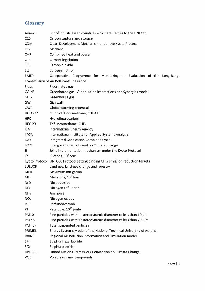
Glossary
Annex I List of industrialized countries which are Parties to the UNFCCC CCS Carbon capture and storage CDM Clean Development Mechanism under the Kyoto Protocol CH4 Methane CHP Combined heat and power CLE Current legislation CO2 Carbon dioxide EU European Union EMEP Co‐operative Programme for Monitoring an Evaluation of the Long‐Range Transmission of Air Pollutants in Europe F‐gas Fluorinated gas GAINS Greenhouse gas ‐ Air pollution Interactions and Synergies model GHG Greenhouse gas GW Gigawatt GWP Global warming potential HCFC‐22 Chlorodifluoromethane, CHF2Cl HFC Hydrofluorocarbon HFC‐23 Trifluoromethane, CHF3 IEA International Energy Agency IIASA International Institute for Applied Systems Analysis IGCC Integrated Gasification Combined Cycle IPCC Intergovernmental Panel on Climate Change JI Joint implementation mechanism under the Kyoto Protocol Kt Kilotons, 103 tons Kyoto Protocol UNFCCC Protocol setting binding GHG emission reduction targets LULUCF Land use, land‐use change and forestry MFR Maximum mitigation Mt Megatons, 106 tons N2O Nitrous oxide NF3 Nitrogen trifluoride NH3 Ammonia NOx Nitrogen oxides PFC Perfluorocarbon PJ Petajoule, 1015 joule PM10 Fine particles with an aerodynamic diameter of less than 10 μm PM2.5 Fine particles with an aerodynamic diameter of less than 2.5 μm PM TSP Total suspended particles PRIMES Energy Systems Model of the National Technical University of Athens RAINS Regional Air Pollution Information and Simulation model SF6 Sulphur hexafluoride SO2 Sulphur dioxide UNFCCC United Nations Framework Convention on Climate Change VOC Volatile organic compounds
Page | 6
How this guide is organized
Some introductions to web interface systems are like reference manuals: they describe each command in detail. Others take you step by step through a small number of examples. This user’s guide contains elements of both approaches with information structured into three distinctive parts:
The first part is introductory. It gives a brief explanation for what the model can be used for, what are general principals and objectives. It also outlines the scope of the tool. It will help you to understand the basic features of the GAINS web interface and to proceed with accessing the online tool. Furthermore, it will guide you through the elements of the web interface and steps of importing data from the model with the help of many examples and numerous screen‐snapshots. Examples are demonstrated within the GAINS‐Europe scheme through the country of Austria. The first part also serves as a tutorial for those model users, who want to view assumptions and results of scenarios that were prepared by IIASA and are in the public domain. That group of users has VIEWER privileges.
The second part is for those with USER privileges. This group of model users has the right to create in GAINS scenarios under their own ownership. The tutorial briefly describes advanced data management functions and editors, like creation of new input data and organizing the new data sets into an emission scenario. All operations are illustrated through a series of screen shots, which provide guidance about operations that need to be done and their sequence.
Finally, the third part provides a description of the aggregation of the GAINS energy database. In particular, it discusses the aggregation of energy carriers and economic sectors in GAINS energy balances and briefly discuses data sources used.
Page | 7
PART I – Getting started: deriving and using data __________________________________________________________________________________
1 Introduction
The Greenhouse Gas and Air Pollution Interactions and Synergies (GAINS) model is an integrated assessment model dealing with costs and potentials for air pollution control and greenhouse gas (GHG) mitigation, and assessing interactions between policies.
The GAINS model grew out of the RAINS model, which has been developed by the IIASA APD Programme over some 20 years. The RAINS model is an air pollution emission and impact model that helps in analysis of policy implications of controlling emissions of major air pollutants (SO2, NOX, VOC, PM, NH3) at the national and international scales. The model identifies air pollution impacts (acidification, eutrophication, ozone, human health) and helps in preparation of cost‐efficient pollution control strategies.
GAINS is an extension of the RAINS model to include major greenhouse gases, i.e. CO2, CH4, N2O and the F‐gases. This makes it possible to simultaneously analyze the effects of mitigation of greenhouse gases emissions and air pollution. In this way the most important interactions and synergies between the mitigation of climate relevant gases and air pollution can be studied.
The purpose of this tutorial is to give an introduction on the basic concept of the GAINS model and to guide model users through the online model interface. No special analytical skills or advanced knowledge in environmental and social sciences is required to use either the web interface or this guide. We hope that it will be useful for researchers, policy advisors, journalists, and students who are interested in quantitative analysis of issues covered by the model.
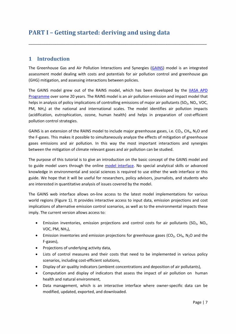
The GAINS web interface allows on‐line access to the latest model implementations for various world regions (Figure 1). It provides interactive access to input data, emission projections and cost implications of alternative emission control scenarios, as well as to the environmental impacts these imply. The current version allows access to:
• Emission inventories, emission projections and control costs for air pollutants (SO2, NOX, VOC, PM, NH3),
• Emission inventories and emission projections for greenhouse gases (CO2, CH4, N2O and the F‐gases),
• Projections of underlying activity data,
• Lists of control measures and their costs that need to be implemented in various policy scenarios, including cost‐efficient solutions,
• Display of air quality indicators (ambient concentrations and deposition of air pollutants),
• Computation and display of indicators that assess the impact of air pollution on human health and natural environment,
• Data management, which is an interactive interface where owner‐specific data can be modified, updated, exported, and downloaded.

Page | 8
The GAINS Model addresses health and ecosystem impacts of particulate pollution, acidification, eutrophication of ecosystems, and impacts of tropospheric ozone. Simultaneously, GAINS assesses the effects of various scenarios on greenhouse gases mitigation and the resulting co‐benefits for air pollution. Historic emissions of air pollutants and GHGs are estimated for each country based on international emission inventories and statistics as well as on inputs from collaborating national expert teams. Emissions are assessed on a medium‐term time horizon up to the year 2030 with five year intervals.
Options and costs for controlling emissions are represented by several emission reduction technologies. Atmospheric dispersion processes are often modeled exogenously and integrated into the GAINS Model framework. Critical load data and critical level data are often compiled exogenously and incorporated into the GAINS modeling framework.
The model can be operated in the 'scenario analysis' mode, i.e., following the pathways of the emissions from their sources to their impacts. In this case the model provides estimates of regional costs and environmental benefits of alternative emission control strategies. The Model can also operate in the 'optimization mode' which identifies cost‐optimal allocations of emission reductions in order to achieve specified deposition levels, concentration targets, or GHG emissions ceilings. The current version of the model can be used for viewing activity levels and emission control strategies, as well as calculating emissions and control costs for those strategies.
All results are calculated on the fly to ensure that the most recent data set is used at all times. The interface enables display and download of all input data and scenario results.
2 Accessing GAINS online This GAINS portal provides access to the on‐line implementations of the GAINS model for various groups of countries and parts or the world, as well as to supporting documentation material. In particular, the model can be assessed for Annex I countries of the UNFCCC Convention, for Europe, China, Southeast Asia, and for the rest of the world.
Hardware and software requirements of the tool We recommend having one of the latest browsers installed on your computer installed with JAVA software. You will need a regular PC or Mac with no special capabilities to start using GAINS. The GAINS model is accessible through any web browser software (Mozilla Firefox, Opera, Microsoft Internet Explorer). Access is free. For technical reasons a one‐time registration is required, after which a password will be sent automatically via e‐mail.
By default, users are granted VIEWER permission for displaying and downloading all data (subject to acceptance of the disclaimer and licensing conditions). USER permissions to upload data are granted to collaborators on demand. The first part of this guide can be considered as the tutorial for users with VIEWER status and the second part provides the tutorial on operations for those who are granted with USER privileges.
The web interface of the GAINS model can be accessed from the home page of the IIASA APD, or directly through the following link: http://gains.iiasa.ac.at/index.php/home‐page/241‐on‐line‐access‐to‐gains. The start page of the web site will look like in the Figure 1:
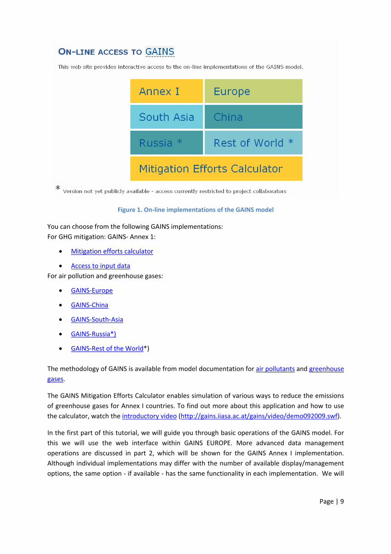
Figure 1. On‐line implementations of the GAINS model
You can choose from the following GAINS implementations: For GHG mitigation: GAINS‐ Annex 1:
• Mitigation efforts calculator
• Access to input data For air pollution and greenhouse gases:
• GAINS‐Europe
• GAINS‐China
• GAINS‐South‐Asia
• GAINS‐Russia*)
• GAINS‐Rest of the World*) The methodology of GAINS is available from model documentation for air pollutants and greenhouse gases.
The GAINS Mitigation Efforts Calculator enables simulation of various ways to reduce the emissions of greenhouse gases for Annex I countries. To find out more about this application and how to use the calculator, watch the introductory video (http://gains.iiasa.ac.at/gains/video/demo092009.swf).
In the first part of this tutorial, we will guide you through basic operations of the GAINS model. For this we will use the web interface within GAINS EUROPE. More advanced data management operations are discussed in part 2, which will be shown for the GAINS Annex I implementation. Although individual implementations may differ with the number of available display/management options, the same option ‐ if available ‐ has the same functionality in each implementation. We will
Page | 9
demonstrate how GAINS operates by examples. All numeric examples (tables with input data and results) will be demonstrated for Austria.
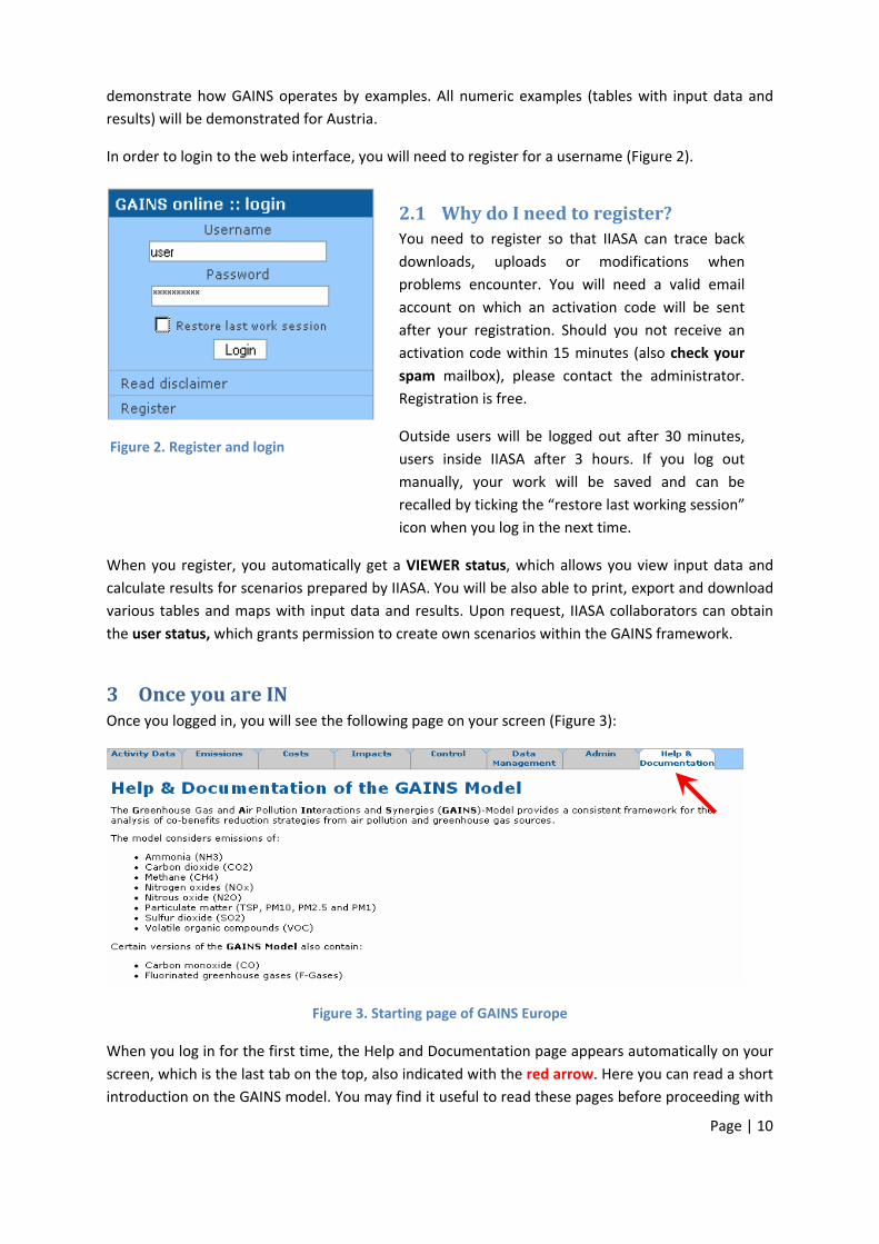
In order to login to the web interface, you will need to register for a username (Figure 2).
Figure 2. Register and login
2.1 Why do I need to register? You need to register so that IIASA can trace back downloads, uploads or modifications when problems encounter. You will need a valid email account on which an activation code will be sent after your registration. Should you not receive an activation code within 15 minutes (also check your spam mailbox), please contact the administrator. Registration is free.
Outside users will be logged out after 30 minutes, users inside IIASA after 3 hours. If you log out manually, your work will be saved and can be recalled by ticking the “restore last working session” icon when you log in the next time.
When you register, you automatically get a VIEWER status, which allows you view input data and calculate results for scenarios prepared by IIASA. You will be also able to print, export and download various tables and maps with input data and results. Upon request, IIASA collaborators can obtain the user status, which grants permission to create own scenarios within the GAINS framework.
3 Once you are IN Once you logged in, you will see the following page on your screen (Figure 3):
Figure 3. Starting page of GAINS Europe
When you log in for the first time, the Help and Documentation page appears automatically on your screen, which is the last tab on the top, also indicated with the red arrow. Here you can read a short introduction on the GAINS model. You may find it useful to read these pages before proceeding with
Page | 10
the next steps. On the left side you can also check the Change Log, which lists the most recent changes that have been made in the model.
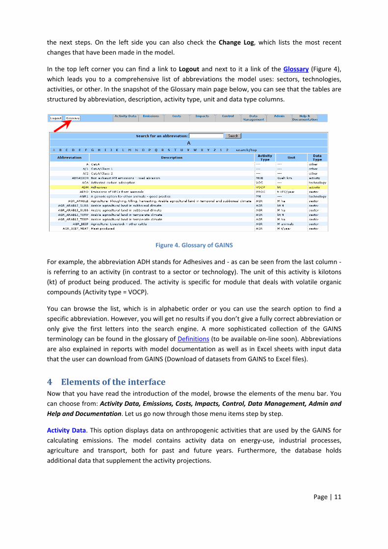
In the top left corner you can find a link to Logout and next to it a link of the Glossary (Figure 4), which leads you to a comprehensive list of abbreviations the model uses: sectors, technologies, activities, or other. In the snapshot of the Glossary main page below, you can see that the tables are structured by abbreviation, description, activity type, unit and data type columns.
Figure 4. Glossary of GAINS
For example, the abbreviation ADH stands for Adhesives and ‐ as can be seen from the last column ‐is referring to an activity (in contrast to a sector or technology). The unit of this activity is kilotons (kt) of product being produced. The activity is specific for module that deals with volatile organic compounds (Activity type = VOCP).
You can browse the list, which is in alphabetic order or you can use the search option to find a specific abbreviation. However, you will get no results if you don’t give a fully correct abbreviation or only give the first letters into the search engine. A more sophisticated collection of the GAINS terminology can be found in the glossary of Definitions (to be available on‐line soon). Abbreviations are also explained in reports with model documentation as well as in Excel sheets with input data that the user can download from GAINS (Download of datasets from GAINS to Excel files).
4 Elements of the interface Now that you have read the introduction of the model, browse the elements of the menu bar. You can choose from: Activity Data, Emissions, Costs, Impacts, Control, Data Management, Admin and Help and Documentation. Let us go now through those menu items step by step.
Activity Data. This option displays data on anthropogenic activities that are used by the GAINS for calculating emissions. The model contains activity data on energy‐use, industrial processes, agriculture and transport, both for past and future years. Furthermore, the database holds additional data that supplement the activity projections.
Page | 11
Emissions option displays air pollutants and greenhouse gases emissions for selected scenarios and countries. These emissions can be displayed in various aggregations. From this option one can also display details on the emission‐relevant input data used for the calculations.
Costs option displays emission control costs computed by the GAINS model for a selected emission scenario and provides details on the cost‐relevant input data used for the calculations.
Choosing Impacts one can display computed air quality and the resulting health and environmental impacts of selected emission control scenarios in graphical (maps) and numerical form (tables with country‐specific data).
With the Control option you can view assumptions about controlling emissions in GAINS scenarios. The “View Control Strategies” option gives information about the structure of each emission scenario. You learn what combination of activity assumptions (activity pathway) control measures (control strategy) and emission factors (emission vector) is used in a given scenario for calculating emissions. The “View Control Strategies” option provides information on the uptake of emission control technology adopted in a given strategy to reduce emissions from a given sector.
The Data Management option provides tools for data modification and management. For users with VIEWER privileges only download of input data to GAINS calculations (divided into activity data, control strategies and regional parameters) is available. Upload of data requires USER privileges.
Admin directory contains tools that are important for model administration. Majority of them are reserved for selected IIASA staff. Using this option, VIEWER can change his personal data (email address, password, etc.)
5 Example: display a table with emission data
5.1 Selection of the desired output type
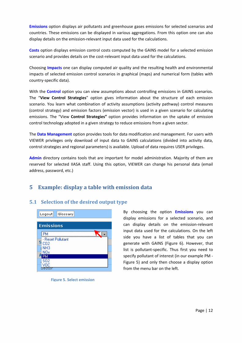
By choosing the option Emissions you can display emissions for a selected scenario, and can display details on the emission‐relevant input data used for the calculations. On the left side you have a list of tables that you can generate with GAINS (Figure 6). However, that list is pollutant‐specific. Thus first you need to specify pollutant of interest (in our example PM ‐
) and only then choose a display option from the menu bar on the left. Figure 5
Figure 5. Select emission
Page | 12
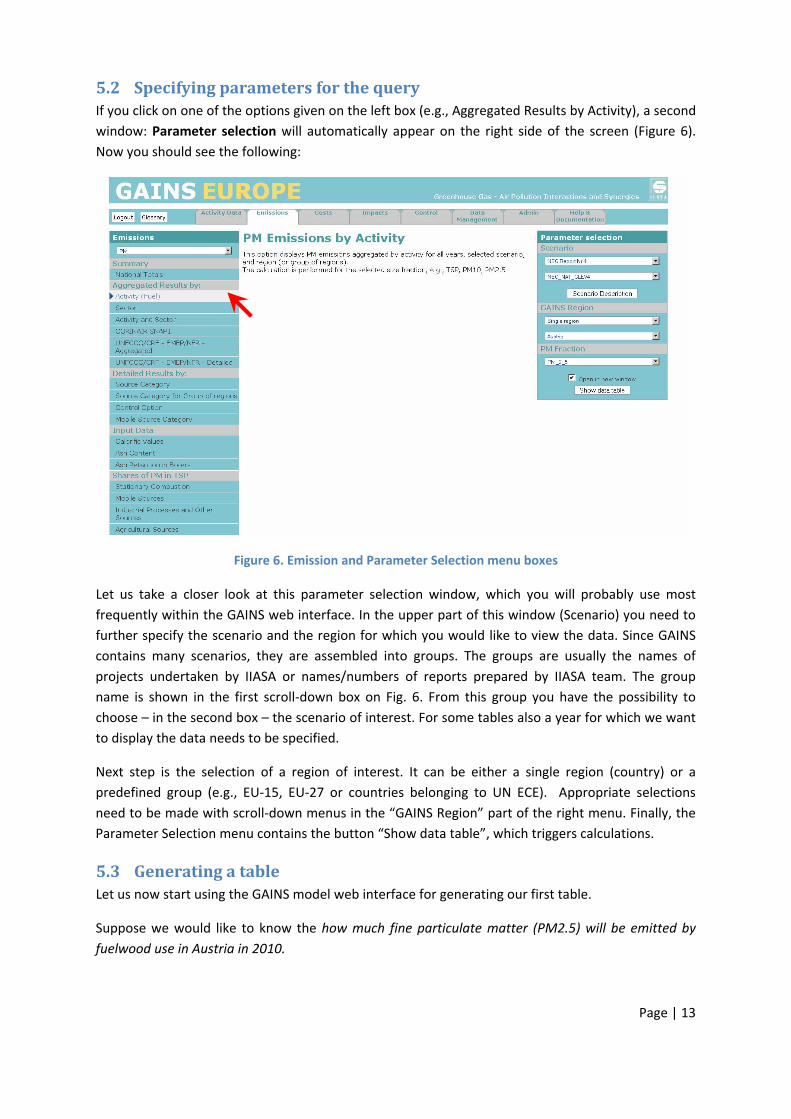
5.2 Specifying parameters for the query If you click on one of the options given on the left box (e.g., Aggregated Results by Activity), a second window: Parameter selection will automatically appear on the right side of the screen (Figure 6). Now you should see the following:
Figure 6. Emission and Parameter Selection menu boxes
Let us take a closer look at this parameter selection window, which you will probably use most frequently within the GAINS web interface. In the upper part of this window (Scenario) you need to further specify the scenario and the region for which you would like to view the data. Since GAINS contains many scenarios, they are assembled into groups. The groups are usually the names of projects undertaken by IIASA or names/numbers of reports prepared by IIASA team. The group name is shown in the first scroll‐down box on Fig. 6. From this group you have the possibility to choose – in the second box – the scenario of interest. For some tables also a year for which we want to display the data needs to be specified.
Next step is the selection of a region of interest. It can be either a single region (country) or a predefined group (e.g., EU‐15, EU‐27 or countries belonging to UN ECE). Appropriate selections need to be made with scroll‐down menus in the “GAINS Region” part of the right menu. Finally, the Parameter Selection menu contains the button “Show data table”, which triggers calculations.
5.3 Generating a table Let us now start using the GAINS model web interface for generating our first table.
Suppose we would like to know the how much fine particulate matter (PM2.5) will be emitted by fuelwood use in Austria in 2010.
Page | 13
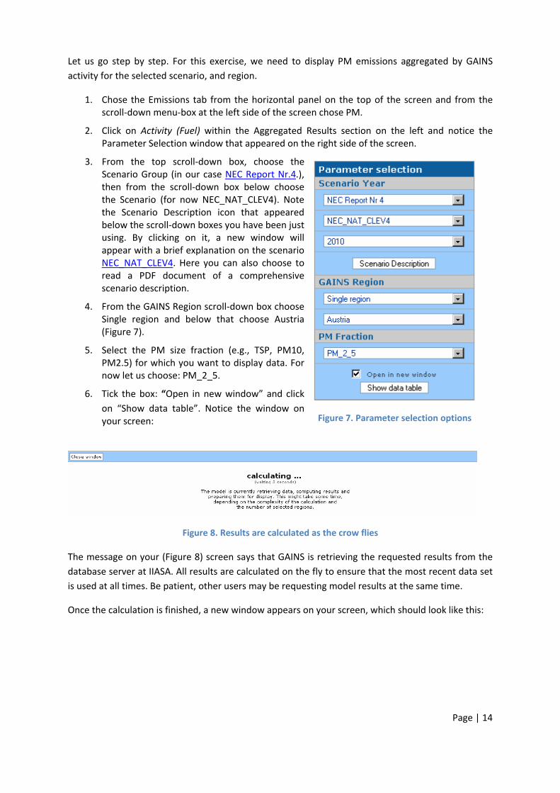
Let us go step by step. For this exercise, we need to display PM emissions aggregated by GAINS activity for the selected scenario, and region.
1. Chose the Emissions tab from the horizontal panel on the top of the screen and from the scroll‐down menu‐box at the left side of the screen chose PM.
2. Click on Activity (Fuel) within the Aggregated Results section on the left and notice the Parameter Selection window that appeared on the right side of the screen.
3. From the top scroll‐down box, choose the Scenario Group (in our case NEC Report Nr.4.), then from the scroll‐down box below choose the Scenario (for now NEC_NAT_CLEV4). Note the Scenario Description icon that appeared below the scroll‐down boxes you have been just using. By clicking on it, a new window will appear with a brief explanation on the scenario NEC_NAT_CLEV4. Here you can also choose to read a PDF document of a comprehensive scenario description.
4. From the GAINS Region scroll‐down box choose Single region and below that choose Austria ( ). Figure 7
5. Select the PM size fraction (e.g., TSP, PM10, PM2.5) for which you want to display data. For now let us choose: PM_2_5.
6. Tick the box: “Open in new window” and click on “Show data table”. Notice the window on your screen: Figure 7. Parameter selection options
Figure 8. Results are calculated as the crow flies
The message on your (Figure 8) screen says that GAINS is retrieving the requested results from the database server at IIASA. All results are calculated on the fly to ensure that the most recent data set is used at all times. Be patient, other users may be requesting model results at the same time.
Once the calculation is finished, a new window appears on your screen, which should look like this:
Page | 14
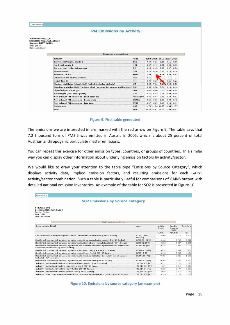
Figure 9. First table generated
The emissions we are interested in are marked with the red arrow on Figure 9. The table says that 7.2 thousand tons of PM2.5 was emitted in Austria in 2005, which is about 25 percent of total Austrian anthropogenic particulate matter emissions.
You can repeat this exercise for other emission types, countries, or groups of countries. In a similar way you can display other information about underlying emission factors by activity/sector.
We would like to draw your attention to the table type “Emissions by Source Category”, which displays activity data, implied emission factors, and resulting emissions for each GAINS activity/sector combination. Such a table is particularly useful for comparisons of GAINS output with detailed national emission inventories. An example of the table for SO2 is presented in Figure 10.
Figure 10. Emissions by source category (an example)
Page | 15
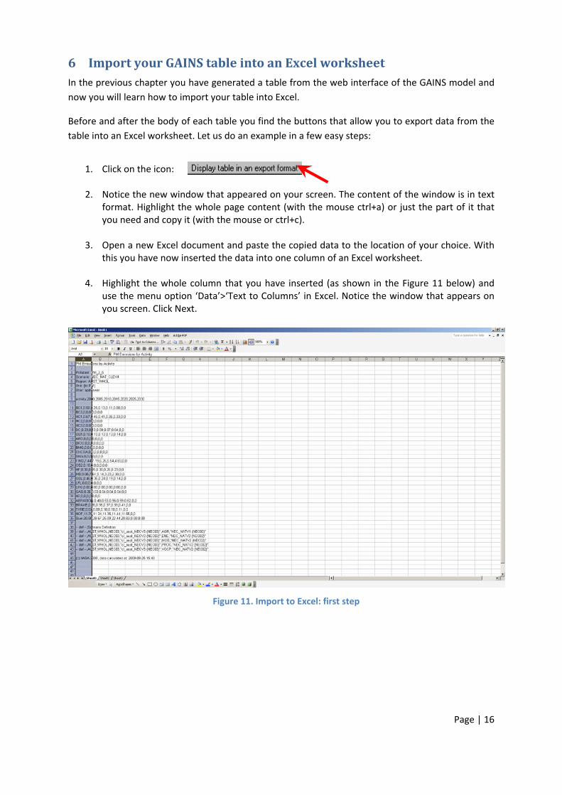
6 Import your GAINS table into an Excel worksheet In the previous chapter you have generated a table from the web interface of the GAINS model and now you will learn how to import your table into Excel.
Before and after the body of each table you find the buttons that allow you to export data from the table into an Excel worksheet. Let us do an example in a few easy steps:
1. Click on the icon: 2. Notice the new window that appeared on your screen. The content of the window is in text
format. Highlight the whole page content (with the mouse ctrl+a) or just the part of it that you need and copy it (with the mouse or ctrl+c).
3. Open a new Excel document and paste the copied data to the location of your choice. With
this you have now inserted the data into one column of an Excel worksheet.
4. Highlight the whole column that you have inserted (as shown in the below) and use the menu option ‘Data’>‘Text to Columns’ in Excel. Notice the window that appears on you screen. Click Next.
Figure 11
Figure 11. Import to Excel: first step
Page | 16
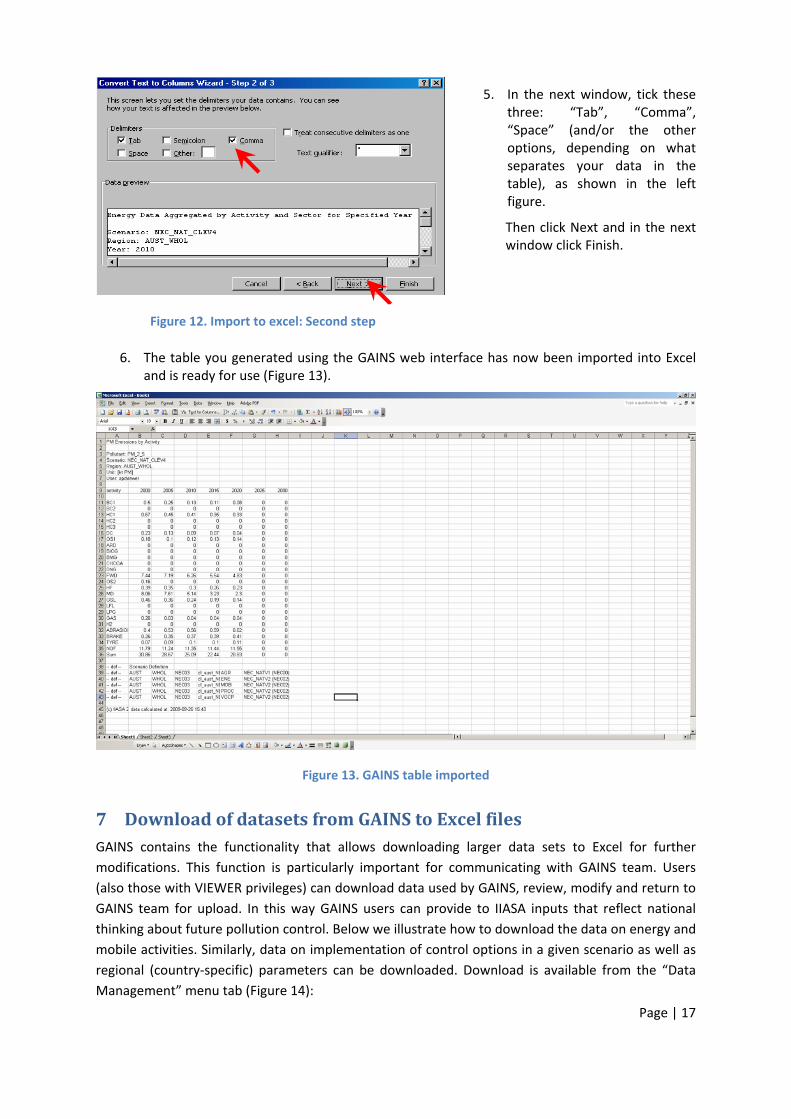
5. In the next window, tick these three: “Tab”, “Comma”, “Space” (and/or the other options, depending on what separates your data in the table), as shown in the left figure.
Then click Next and in the next window click Finish.
Figure 12. Import to excel: Second step
6. The table you generated using the GAINS web interface has now been imported into Excel and is ready for use (Figure 13).
Figure 13. GAINS table imported
7 Download of datasets from GAINS to Excel files GAINS contains the functionality that allows downloading larger data sets to Excel for further modifications. This function is particularly important for communicating with GAINS team. Users (also those with VIEWER privileges) can download data used by GAINS, review, modify and return to GAINS team for upload. In this way GAINS users can provide to IIASA inputs that reflect national thinking about future pollution control. Below we illustrate how to download the data on energy and mobile activities. Similarly, data on implementation of control options in a given scenario as well as regional (country‐specific) parameters can be downloaded. Download is available from the “Data Management” menu tab (Figure 14):
Page | 17
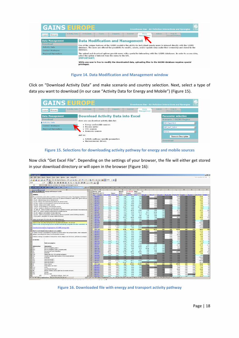
Figure 14. Data Modification and Management window
Click on “Download Activity Data” and make scenario and country selection. Next, select a type of data you want to download (in our case “Activity Data for Energy and Mobile”) (Figure 15).
Figure 15. Selections for downloading activity pathway for energy and mobile sources
Now click “Get Excel File”. Depending on the settings of your browser, the file will either get stored in your download directory or will open in the browser (Figure 16):
Figure 16. Downloaded file with energy and transport activity pathway
Page | 18
Page | 19
Such a file can be checked by national experts and modified/corrected, if necessary. Corrections need to be sent to IIASA for implementation. However, modifications cannot violate the structure of the GAINS database. Detailed description of the contents of the file, together with the rules for modification is included in the “Explanations” tab.
8 Produce a map with environmental impacts Let us now display a map using the web interface. Maps are available from the “Impacts” tab. For calculation and displaying of impact indicators GAINS uses results from atmospheric dispersion and chemical transport models (e.g., EMEP http://www.emep.int/OpenSource/index.html, TM5 http://www.phys.uu.nl/~tm5/). Pollution transfer matrices developed on a basis of those models allow calculations of contributions of emissions from each country in the modeling domain to concentrations and/or depositions of air pollutants in particular locations. For Europe, IIASA uses results of the EMEP model and the EMEP model grid (50 x 50 km).
From the impacts module the user can display:
1. Air quality indicators,
2. Concentrations of fine particulate matter (maps and tables) ,
3. Concentrations of ground‐level ozone (tables only) ,
4. Deposition of sulfur and nitrogen compounds (maps and tables) ,
5. Health impacts attributable to PM2.5 exposure (maps and tables) ,
6. Health impact indicators for ground‐level ozone ,
7. Excess of critical loads for acidification and eutrophication, for forests, semi‐natural ecosystems and for freshwater catchment areas.
We will display the losses of statistical life expectancy from exposure to anthropogenic PM2.5 in 2020 following from the “NEC_NAT_CLEV4” scenario.
1. Chose the option Impacts from the horizontal panel on the top of the screen and click the option “Health and Environmental Impacts” in the menu‐box at the left side of the screen.
2. Notice the Parameter Selection window that appeared on the right side of the screen. Choose the map domain Europe and click: “Show map”.
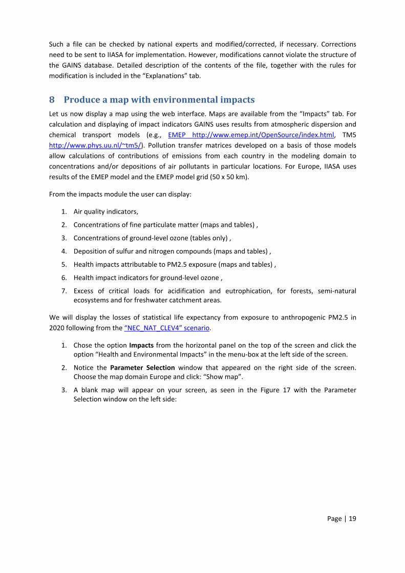
3. A blank map will appear on your screen, as seen in the Figure 17 with the Parameter Selection window on the left side:
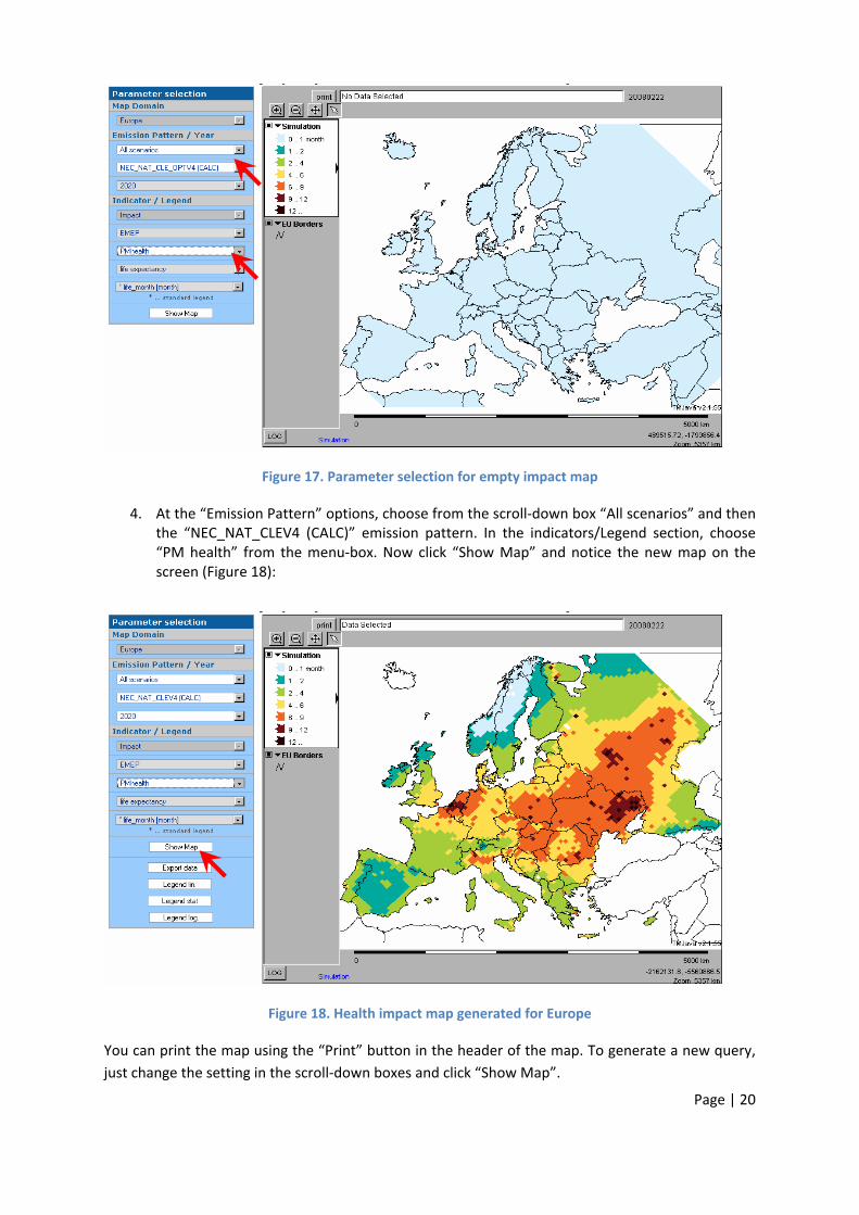
Figure 17. Parameter selection for empty impact map
4. At the “Emission Pattern” options, choose from the scroll‐down box “All scenarios” and then the “NEC_NAT_CLEV4 (CALC)” emission pattern. In the indicators/Legend section, choose “PM health” from the menu‐box. Now click “Show Map” and notice the new map on the screen (Figure 18):
Figure 18. Health impact map generated for Europe
You can print the map using the “Print” button in the header of the map. To generate a new query, just change the setting in the scroll‐down boxes and click “Show Map”.
Page | 20
Page | 21
PART II – Create and edit emission scenarios in GAINS
1 General principles and definitions
One of the unique features of the GAINS model is the ability for individual remote users to interact directly with the GAINS database. The users are offered the possibility to modify, create, and/or update data for GAINS calculations and create their own emission scenarios. To facilitate these operations, GAINS is equipped with several editors and data download/upload possibilities.
In order to better understand the logic behind the structure of the GAINS database, equations (1) and (2) present – in a stylized way ‐ the basic principles of calculating emissions and emission control costs in the model:
Emissions = Activity * Emission factor * Technology implementation (1)
Costs = Activity * Unit cost * Technology implementation (2)
Components appearing on the right side of the equations are organized into three different data categories. Emissions‐generating economic activities are organized into activity pathways. GAINS divides activity data into five groups: Energy (ENE), Mobile sources (MOB), Agriculture (AGR), Process (PROC), and VOC‐specific (VOC)1. Emission factors and unit costs of control technologies, together with all background information, form the so‐called emission vector. Finally, technology implementation for each activity is specified in control strategies2.
Each emission scenario in GAINS is created through a combination of these three data categories:
• activity pathways,
• emission vectors, and
• control strategies.
Every combination determines the level of actual emissions. Data are country‐specific. Structure of the scenario can be always displayed from the model, as described in Section 2.
Each GAINS scenario has its owner. The owner is a person, who has created and named the actual scenario. Only the owner can modify and maintain his scenario3. Creation of a new emission
1 Sixth category: “Buildings” with data used for estimating potentials for energy efficiency improvements in residential and commercial sectors will be added soon. 2 Model aggregation (emitting sectors, control technologies, their efficiencies and costs) is discussed in appropriate methodology papers for air pollution and greenhouse gases:
• CO2 (http://www.iiasa.ac.at/cgi‐bin/pub/pubsrchJJ?SWID:IR05053&O,n)
• Methane (http://www.iiasa.ac.at/cgi‐bin/pub/pubsrchJJ?SWID:IR05054&O,n)
• F‐Gases (http://www.iiasa.ac.at/cgi‐bin/pub/pubsrchJJ?SWID:IR05056&O,n)
• Nitrous Oxide (http://www.iiasa.ac.at/cgi‐bin/pub/pubsrchJJ?SWID:IR05055&O,n) 3 Model administrators can also assign rights to modify (some of) the scenarios to a group of users. However, this group ownership is not discussed in detail in this tutorial.
scenario depends on changing one (or more) scenario components for at least one country. The user can either utilize files already stored in the database, or create new inputs, that reflect own assumptions, and then organize them into the new scenario.
Modification of input data to GAINS is possible through appropriate editing tools. This document describes the most important editors and demonstrates examples of their use.
For the time being, modification of the emission vector is reserved for IIASA staff. If requested, IIASA may create a country‐specific emission vector and grant the rights to modify it to advanced GAINS users. Since they usually have close working relations with IIASA, this tutorial does not explain how to modify the emission vector.
As already discussed in Part I, GAINS users belong to two groups, namely:
• VIEWERS can view input data and generate results in various aggregations for scenarios created by IIASA and available in public domain. They can also download data used in calculations.
• USERS have ‐ in addition – the right to generate own scenarios based on own input data.
Advanced data management and upload functions are available only for USERS. If you want to acquire the USER status, contact GAINS team ([email protected]).
Operations shown in the further part of the document are performed with the login “apduser”, which has the USER rights. With your own login you will have the same display/editing possibilities as apduser.
2 Display the Structure of Emission Scenarios
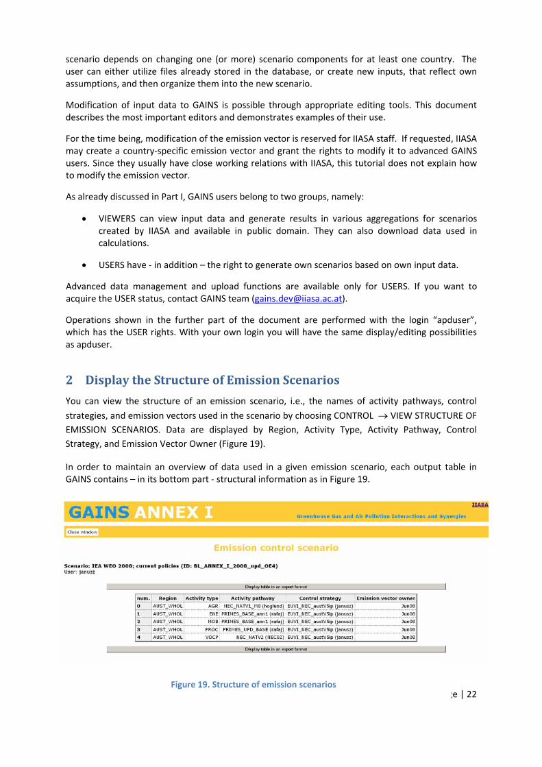
You can view the structure of an emission scenario, i.e., the names of activity pathways, control
strategies, and emission vectors used in the scenario by choosing CONTROL → VIEW STRUCTURE OF EMISSION SCENARIOS. Data are displayed by Region, Activity Type, Activity Pathway, Control Strategy, and Emission Vector Owner ( ). Figure 19
Figure 19In order to maintain an overview of data used in a given emission scenario, each output table in GAINS contains – in its bottom part ‐ structural information as in .
Page | 22
Figure 19. Structure of emission scenarios
3 Workflow
In the rest of this document you will learn how to create an emission scenario under your ownership. For this, we will demonstrate how to create a new activity pathway and a new control strategy and how to combine them into a new emission scenario. The following workflow shows major steps that will be discussed. These are:
1. Creating new emission scenario
2. Creating new activity pathway
3. Creating new control strategy
4. Assigning pathways and control strategies to the scenario
5. Downloading activity data
6. Modifying activity data and uploading the modifications
7. Downloading control strategy
8. Modifying control strategy and uploading the modifications
9. Analyzing the effects of changes introduced.
It is strongly recommended that you follow this sequence when you begin your work with GAINS as USER. Otherwise you might not be able to see the files you created. Each step requires several operations, which will be discussed and explained on examples. Examples are limited to modification of energy sector data and control strategy for SO2. Similar operations can be done for other types of activities and other pollutants. All examples shown in this part of the tutorial have been produced with the implementation of GAINS for Annex I countries.
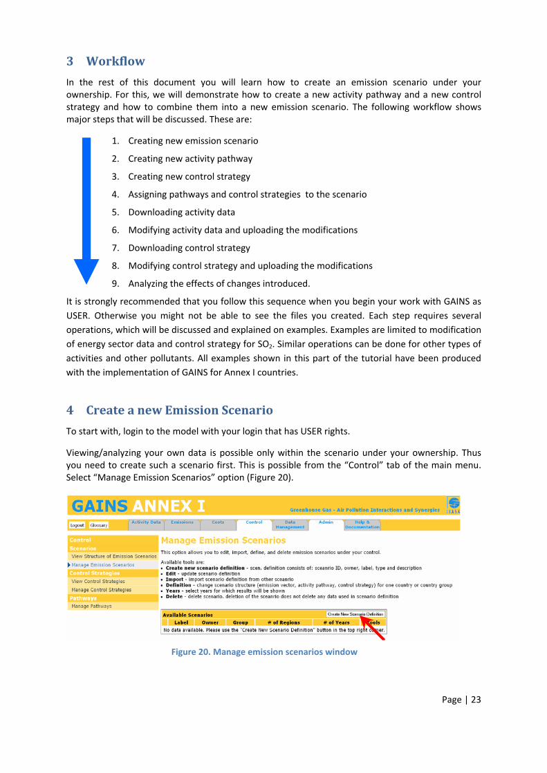
4 Create a new Emission Scenario
To start with, login to the model with your login that has USER rights.
Viewing/analyzing your own data is possible only within the scenario under your ownership. Thus you need to create such a scenario first. This is possible from the “Control” tab of the main menu. Select “Manage Emission Scenarios” option ( ). Figure 20
Figure 20. Manage emission scenarios window
Page | 23
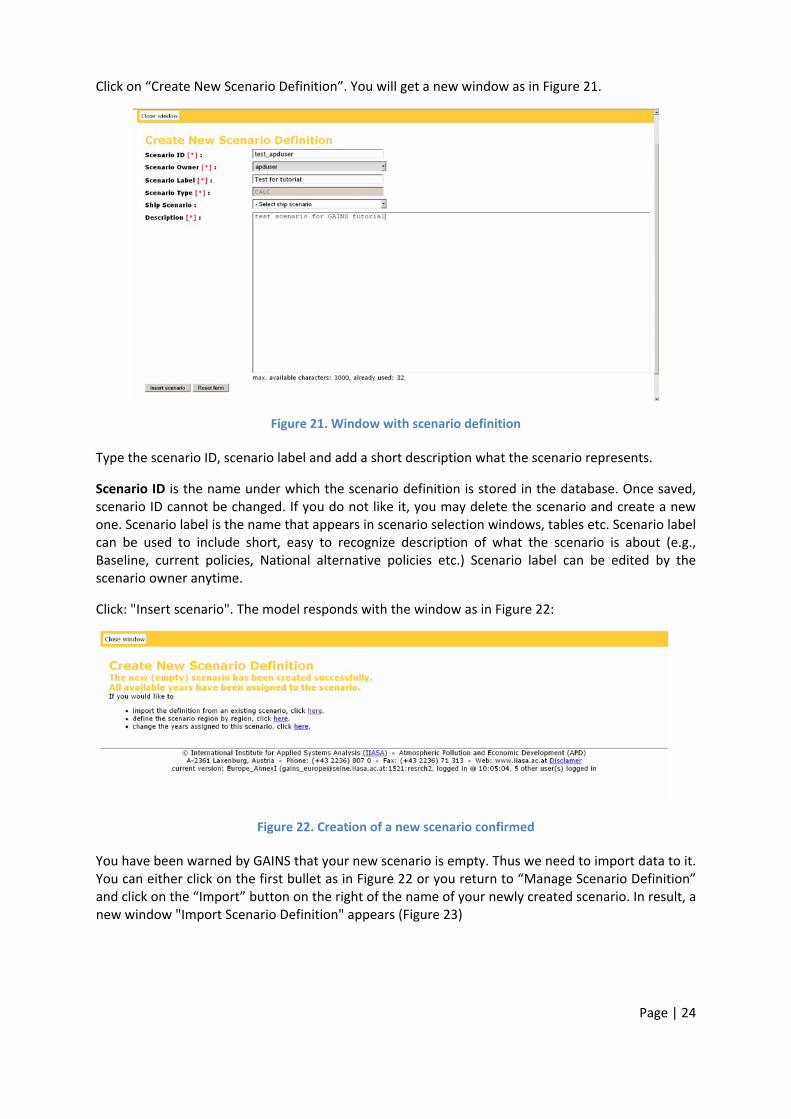
Click on “Create New Scenario Definition”. You will get a new window as in Figure 21.
Figure 21. Window with scenario definition
Type the scenario ID, scenario label and add a short description what the scenario represents.
Scenario ID is the name under which the scenario definition is stored in the database. Once saved, scenario ID cannot be changed. If you do not like it, you may delete the scenario and create a new one. Scenario label is the name that appears in scenario selection windows, tables etc. Scenario label can be used to include short, easy to recognize description of what the scenario is about (e.g., Baseline, current policies, National alternative policies etc.) Scenario label can be edited by the scenario owner anytime.
Click: "Insert scenario". The model responds with the window as in Figure 22:
Figure 22. Creation of a new scenario confirmed
You have been warned by GAINS that your new scenario is empty. Thus we need to import data to it. You can either click on the first bullet as in Figure 22 or you return to “Manage Scenario Definition” and click on the “Import” button on the right of the name of your newly created scenario. In result, a new window "Import Scenario Definition" appears (Figure 23)
Page | 24
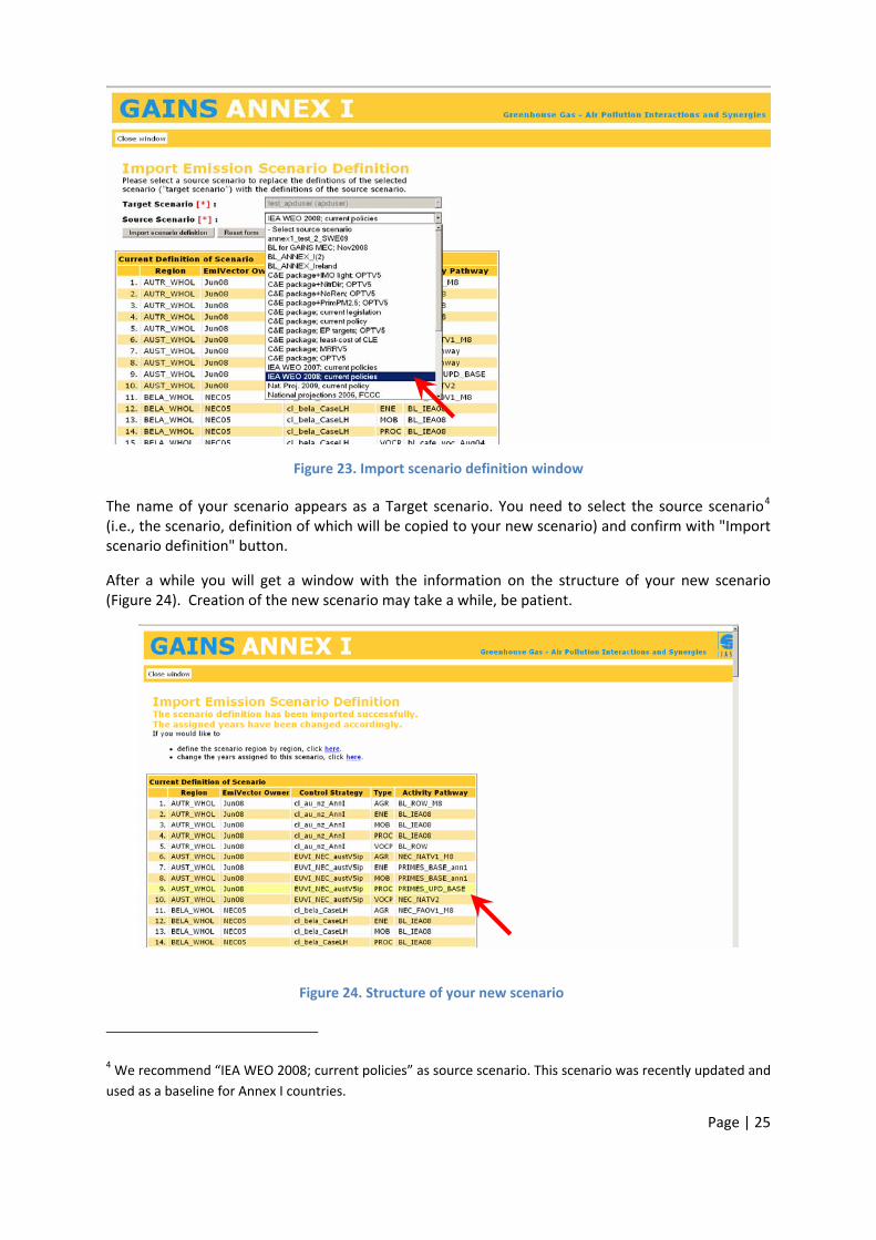
Figure 23. Import scenario definition window
The name of your scenario appears as a Target scenario. You need to select the source scenario4 (i.e., the scenario, definition of which will be copied to your new scenario) and confirm with "Import scenario definition" button.
After a while you will get a window with the information on the structure of your new scenario ( ). Creation of the new scenario may take a while, be patient. Figure 24
Figure 24. Structure of your new scenario
4 We recommend “IEA WEO 2008; current policies” as source scenario. This scenario was recently updated and used as a baseline for Annex I countries.
Page | 25
You may also change a scenario of emissions from international shipping on seas surrounding Europe to be included in calculations of air pollution impacts in Europe for your scenario (pull down button 5 in Figure 21). If you skip this operation then shipping emissions will be identical with those included in the scenario you have imported as a starting point for your own scenario.
Now you are (a proud) owner of the scenario under your ownership. However, remember that it is just a copy of a scenario that already existed in GAINS. The difference is that you have the rights to modify your scenario through replacing its elements with other input data. We will demonstrate how to modify the scenario in Section 7, after we have created activity pathway and control strategy under your ownership.
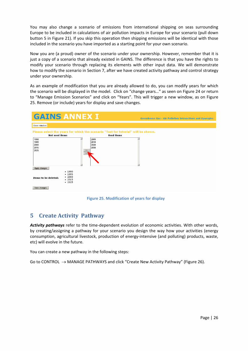
As an example of modification that you are already allowed to do, you can modify years for which the scenario will be displayed in the model. Click on “change years…“ as seen on or return to “Manage Emission Scenarios” and click on “Years”. This will trigger a new window, as on
. Remove (or include) years for display and save changes.
Figure 24Figure
25
Figure 25. Modification of years for display
5 Create Activity Pathway
Activity pathways refer to the time‐dependent evolution of economic activities. With other words, by creating/assigning a pathway for your scenario you design the way how your activities (energy consumption, agricultural livestock, production of energy‐intensive (and polluting) products, waste, etc) will evolve in the future.
You can create a new pathway in the following steps:
Go to CONTROL → MANAGE PATHWAYS and click “Create New Activity Pathway” (Figure 26).
Page | 26
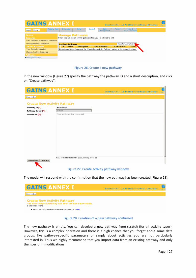
Figure 26. Create a new pathway
In the new window (Figure 27) specify the pathway the pathway ID and a short description, and click on “Create pathway”.
Figure 27. Create activity pathway window
The model will respond with the confirmation that the new pathway has been created (Figure 28):
Figure 28. Creation of a new pathway confirmed
The new pathway is empty. You can develop a new pathway from scratch (for all activity types). However, this is a complex operation and there is a high chance that you forget about some data groups, like pathway‐specific parameters or simply about activities you are not particularly interested in. Thus we highly recommend that you import data from an existing pathway and only then perform modifications.
Page | 27
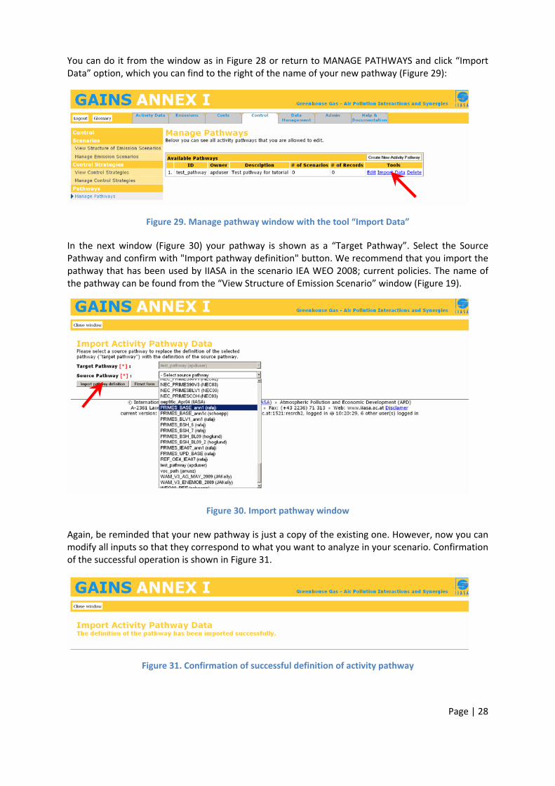
You can do it from the window as in Figure 28 or return to MANAGE PATHWAYS and click “Import Data” option, which you can find to the right of the name of your new pathway (Figure 29):
Figure 29. Manage pathway window with the tool “Import Data”
In the next window (Figure 30) your pathway is shown as a “Target Pathway”. Select the Source Pathway and confirm with "Import pathway definition" button. We recommend that you import the pathway that has been used by IIASA in the scenario IEA WEO 2008; current policies. The name of the pathway can be found from the “View Structure of Emission Scenario” window ( ). Figure 19
Figure 30. Import pathway window
Again, be reminded that your new pathway is just a copy of the existing one. However, now you can modify all inputs so that they correspond to what you want to analyze in your scenario. Confirmation of the successful operation is shown in Figure 31.
Figure 31. Confirmation of successful definition of activity pathway
Page | 28
It needs to be stressed that import has been done for all activity types included in the source pathway. This means that if the source pathway included not only data on energy and mobile sources but also data of “process” type, they were also copied to your new pathway and are available for further modifications. Please note that agricultural pathways and VOC‐specific pathways have usually different names than energy, mobile and process pathways and your new pathway might not contain agricultural and VOC‐specific data. Thus if you want to change activity data for instance for agriculture, you will need to repeat the copy pathway operation for this activity type. If you are not interested in changing agricultural data, you can always use pathways already stored in the GAINS database in your scenario definition.
6 Create Control Strategy
Control strategy is a data set that contains assumptions on the penetration of emission control technologies in a given emission scenario. The complete strategy includes information on controls applied in all sectors for all pollutants. Control strategies “translate” into GAINS legislative packages for emission controls, specifying for each type of emission source (e.g., coal use in the power sector) type and percentage implementation of control technologies required to comply with pollution control legislation (emission standards, sectoral emission ceilings etc.).
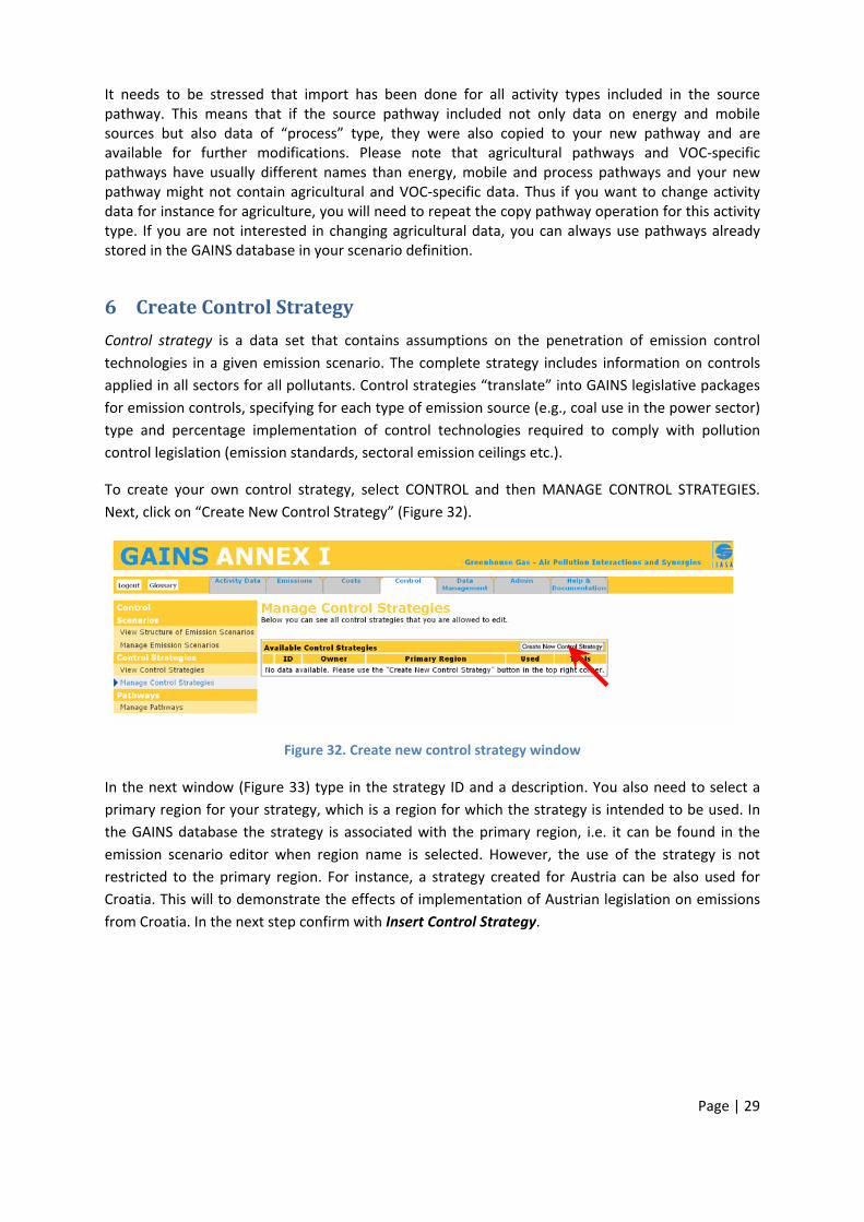
To create your own control strategy, select CONTROL and then MANAGE CONTROL STRATEGIES. Next, click on “Create New Control Strategy” (Figure 32).
Figure 32. Create new control strategy window
In the next window (Figure 33) type in the strategy ID and a description. You also need to select a primary region for your strategy, which is a region for which the strategy is intended to be used. In the GAINS database the strategy is associated with the primary region, i.e. it can be found in the emission scenario editor when region name is selected. However, the use of the strategy is not restricted to the primary region. For instance, a strategy created for Austria can be also used for Croatia. This will to demonstrate the effects of implementation of Austrian legislation on emissions from Croatia. In the next step confirm with Insert Control Strategy.
Page | 29
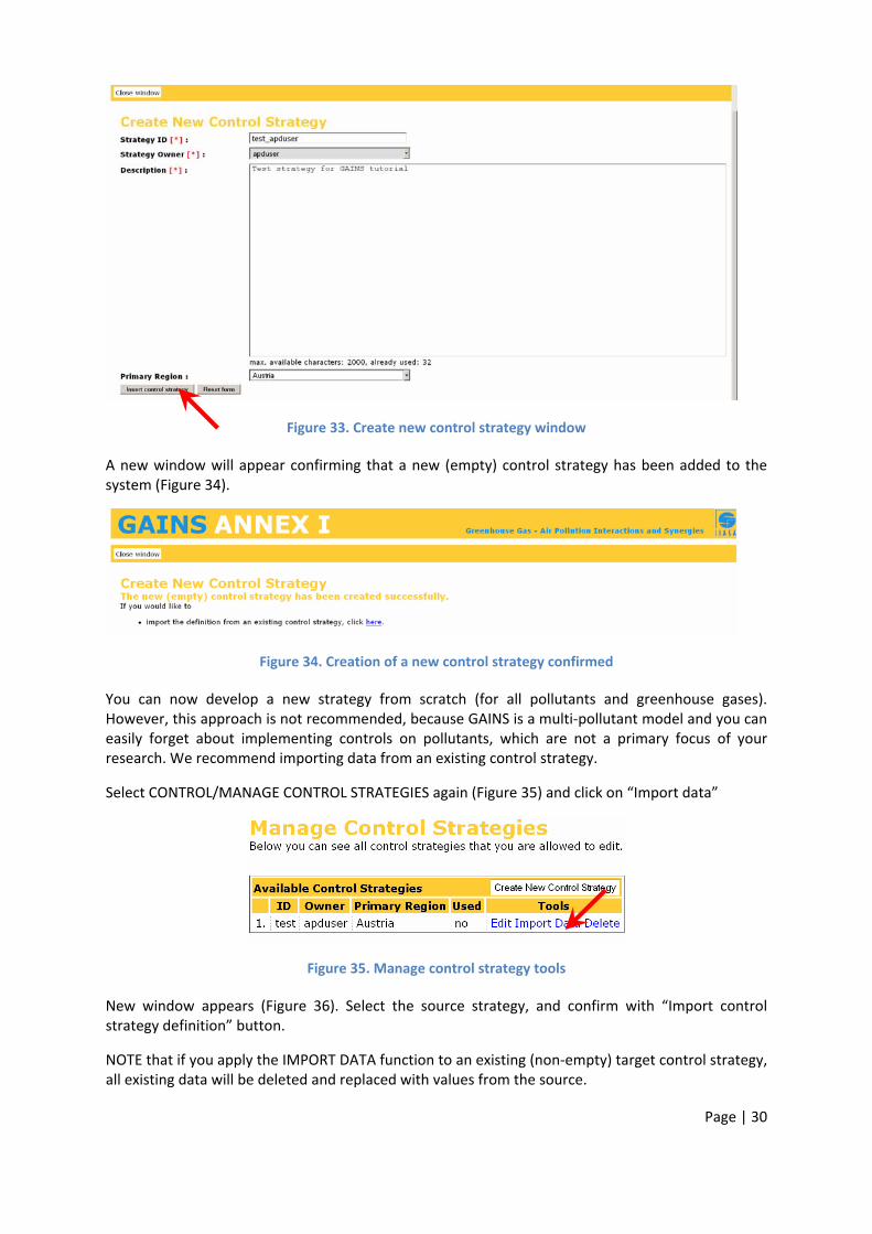
Figure 33. Create new control strategy window
A new window will appear confirming that a new (empty) control strategy has been added to the system (Figure 34).
Figure 34. Creation of a new control strategy confirmed
You can now develop a new strategy from scratch (for all pollutants and greenhouse gases). However, this approach is not recommended, because GAINS is a multi‐pollutant model and you can easily forget about implementing controls on pollutants, which are not a primary focus of your research. We recommend importing data from an existing control strategy.
Select CONTROL/MANAGE CONTROL STRATEGIES again (Figure 35) and click on “Import data”
Figure 35. Manage control strategy tools
New window appears (Figure 36). Select the source strategy, and confirm with “Import control strategy definition” button.
NOTE that if you apply the IMPORT DATA function to an existing (non‐empty) target control strategy, all existing data will be deleted and replaced with values from the source.
Page | 30
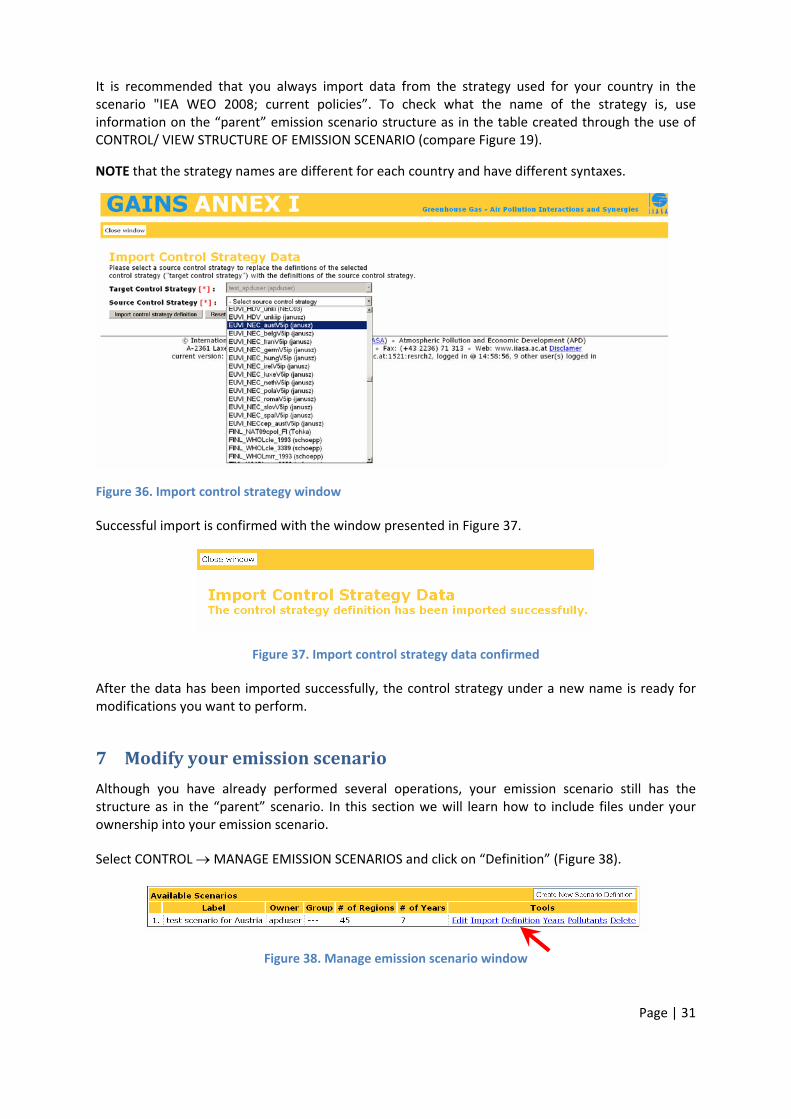
It is recommended that you always import data from the strategy used for your country in the scenario "IEA WEO 2008; current policies”. To check what the name of the strategy is, use information on the “parent” emission scenario structure as in the table created through the use of CONTROL/ VIEW STRUCTURE OF EMISSION SCENARIO (compare ). Figure 19
NOTE that the strategy names are different for each country and have different syntaxes.
Figure 36. Import control strategy window
Successful import is confirmed with the window presented in Figure 37.
Figure 37. Import control strategy data confirmed
After the data has been imported successfully, the control strategy under a new name is ready for modifications you want to perform.
7 Modify your emission scenario
Although you have already performed several operations, your emission scenario still has the structure as in the “parent” scenario. In this section we will learn how to include files under your ownership into your emission scenario.
Select CONTROL → MANAGE EMISSION SCENARIOS and click on “Definition” (Figure 38).
Figure 38. Manage emission scenario window
Page | 31
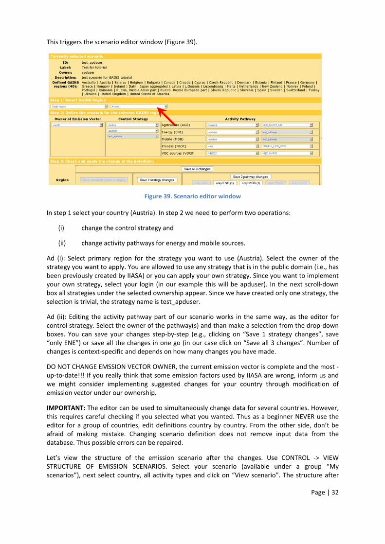
This triggers the scenario editor window (Figure 39).
Figure 39. Scenario editor window
In step 1 select your country (Austria). In step 2 we need to perform two operations:
(i) change the control strategy and
(ii) change activity pathways for energy and mobile sources.
Ad (i): Select primary region for the strategy you want to use (Austria). Select the owner of the strategy you want to apply. You are allowed to use any strategy that is in the public domain (i.e., has been previously created by IIASA) or you can apply your own strategy. Since you want to implement your own strategy, select your login (in our example this will be apduser). In the next scroll‐down box all strategies under the selected ownership appear. Since we have created only one strategy, the selection is trivial, the strategy name is test_apduser.
Ad (ii): Editing the activity pathway part of our scenario works in the same way, as the editor for control strategy. Select the owner of the pathway(s) and than make a selection from the drop‐down boxes. You can save your changes step‐by‐step (e.g., clicking on “Save 1 strategy changes”, save “only ENE”) or save all the changes in one go (in our case click on “Save all 3 changes”. Number of changes is context‐specific and depends on how many changes you have made.
DO NOT CHANGE EMSSION VECTOR OWNER, the current emission vector is complete and the most ‐up‐to‐date!!! If you really think that some emission factors used by IIASA are wrong, inform us and we might consider implementing suggested changes for your country through modification of emission vector under our ownership.
IMPORTANT: The editor can be used to simultaneously change data for several countries. However, this requires careful checking if you selected what you wanted. Thus as a beginner NEVER use the editor for a group of countries, edit definitions country by country. From the other side, don’t be afraid of making mistake. Changing scenario definition does not remove input data from the database. Thus possible errors can be repaired.
Let’s view the structure of the emission scenario after the changes. Use CONTROL ‐> VIEW STRUCTURE OF EMISSION SCENARIOS. Select your scenario (available under a group “My scenarios”), next select country, all activity types and click on “View scenario”. The structure after
Page | 32
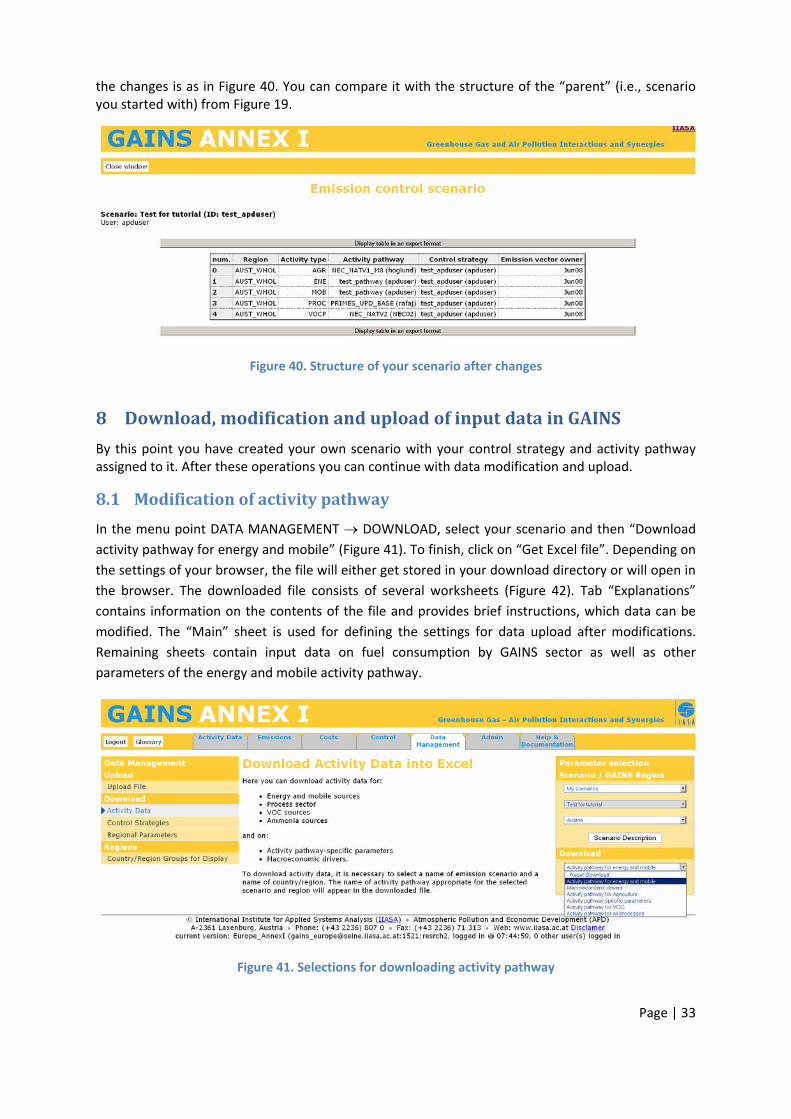
the changes is as in Figure 40. You can compare it with the structure of the “parent” (i.e., scenario you started with) from . Figure 19
Figure 40. Structure of your scenario after changes
8 Download, modification and upload of input data in GAINS
By this point you have created your own scenario with your control strategy and activity pathway assigned to it. After these operations you can continue with data modification and upload.
8.1 Modification of activity pathway In the menu point DATA MANAGEMENT → DOWNLOAD, select your scenario and then “Download activity pathway for energy and mobile” (Figure 41). To finish, click on “Get Excel file”. Depending on the settings of your browser, the file will either get stored in your download directory or will open in the browser. The downloaded file consists of several worksheets (Figure 42). Tab “Explanations” contains information on the contents of the file and provides brief instructions, which data can be modified. The “Main” sheet is used for defining the settings for data upload after modifications. Remaining sheets contain input data on fuel consumption by GAINS sector as well as other parameters of the energy and mobile activity pathway.
Figure 41. Selections for downloading activity pathway
Page | 33
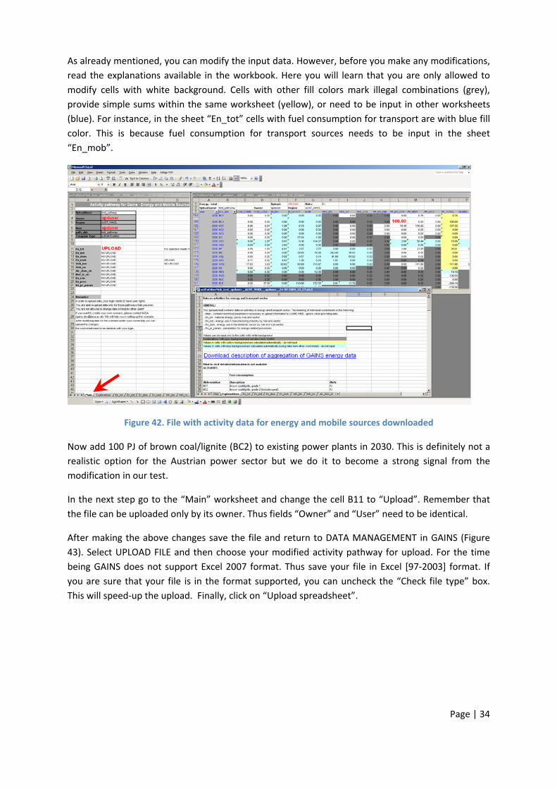
As already mentioned, you can modify the input data. However, before you make any modifications, read the explanations available in the workbook. Here you will learn that you are only allowed to modify cells with white background. Cells with other fill colors mark illegal combinations (grey), provide simple sums within the same worksheet (yellow), or need to be input in other worksheets (blue). For instance, in the sheet “En_tot” cells with fuel consumption for transport are with blue fill color. This is because fuel consumption for transport sources needs to be input in the sheet “En_mob”.
Figure 42. File with activity data for energy and mobile sources downloaded
Now add 100 PJ of brown coal/lignite (BC2) to existing power plants in 2030. This is definitely not a realistic option for the Austrian power sector but we do it to become a strong signal from the modification in our test.
In the next step go to the “Main” worksheet and change the cell B11 to “Upload”. Remember that the file can be uploaded only by its owner. Thus fields “Owner” and “User” need to be identical.
After making the above changes save the file and return to DATA MANAGEMENT in GAINS (Figure 43). Select UPLOAD FILE and then choose your modified activity pathway for upload. For the time being GAINS does not support Excel 2007 format. Thus save your file in Excel [97‐2003] format. If you are sure that your file is in the format supported, you can uncheck the “Check file type” box. This will speed‐up the upload. Finally, click on “Upload spreadsheet”.
Page | 34
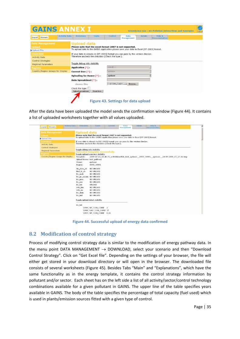
Figure 43. Settings for data upload
After the data have been uploaded the model sends the confirmation window (Figure 44). It contains a list of uploaded worksheets together with all values uploaded.
Figure 44. Successful upload of energy data confirmed
8.2 Modification of control strategy Process of modifying control strategy data is similar to the modification of energy pathway data. In
the menu point DATA MANAGEMENT → DOWNLOAD, select your scenario and then “Download Control Strategy”. Click on “Get Excel file”. Depending on the settings of your browser, the file will either get stored in your download directory or will open in the browser. The downloaded file consists of several worksheets (Figure 45). Besides Tabs “Main” and “Explanations”, which have the same functionality as in the energy template, it contains the control strategy information by pollutant and/or sector. Each sheet has on the left side a list of all activity/sector/control technology combinations available for a given pollutant in GAINS. The upper line of the table specifies years available in GAINS. The body of the table specifies the percentage of total capacity (fuel used) which is used in plants/emission sources fitted with a given type of control.
Page | 35
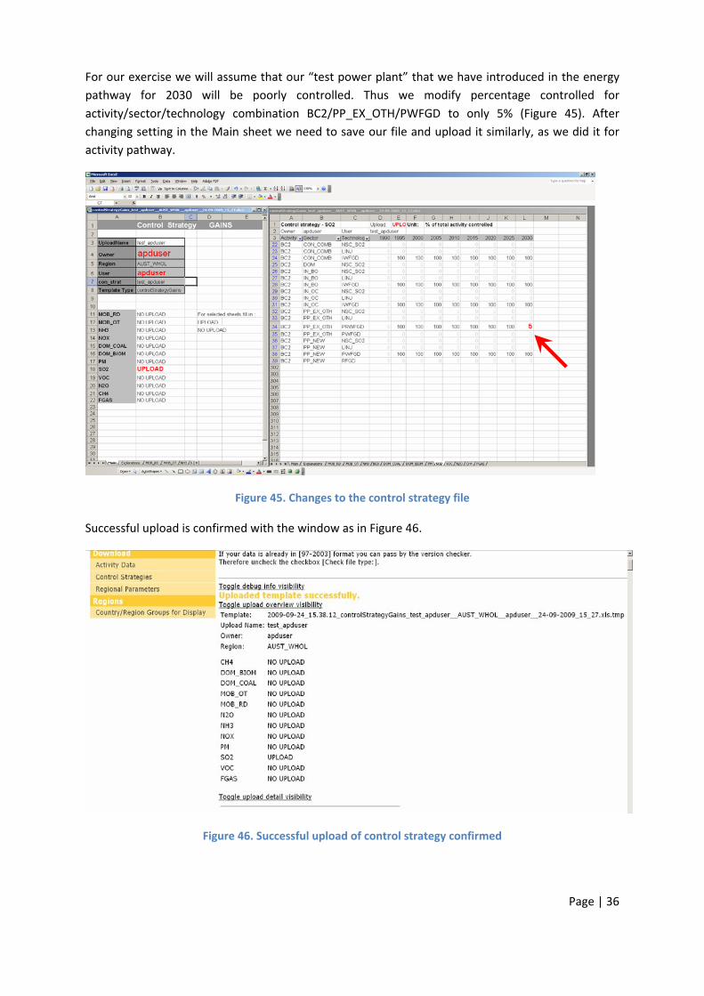
For our exercise we will assume that our “test power plant” that we have introduced in the energy pathway for 2030 will be poorly controlled. Thus we modify percentage controlled for activity/sector/technology combination BC2/PP_EX_OTH/PWFGD to only 5% (Figure 45). After changing setting in the Main sheet we need to save our file and upload it similarly, as we did it for activity pathway.
Figure 45. Changes to the control strategy file
Successful upload is confirmed with the window as in Figure 46.
Figure 46. Successful upload of control strategy confirmed
Page | 36
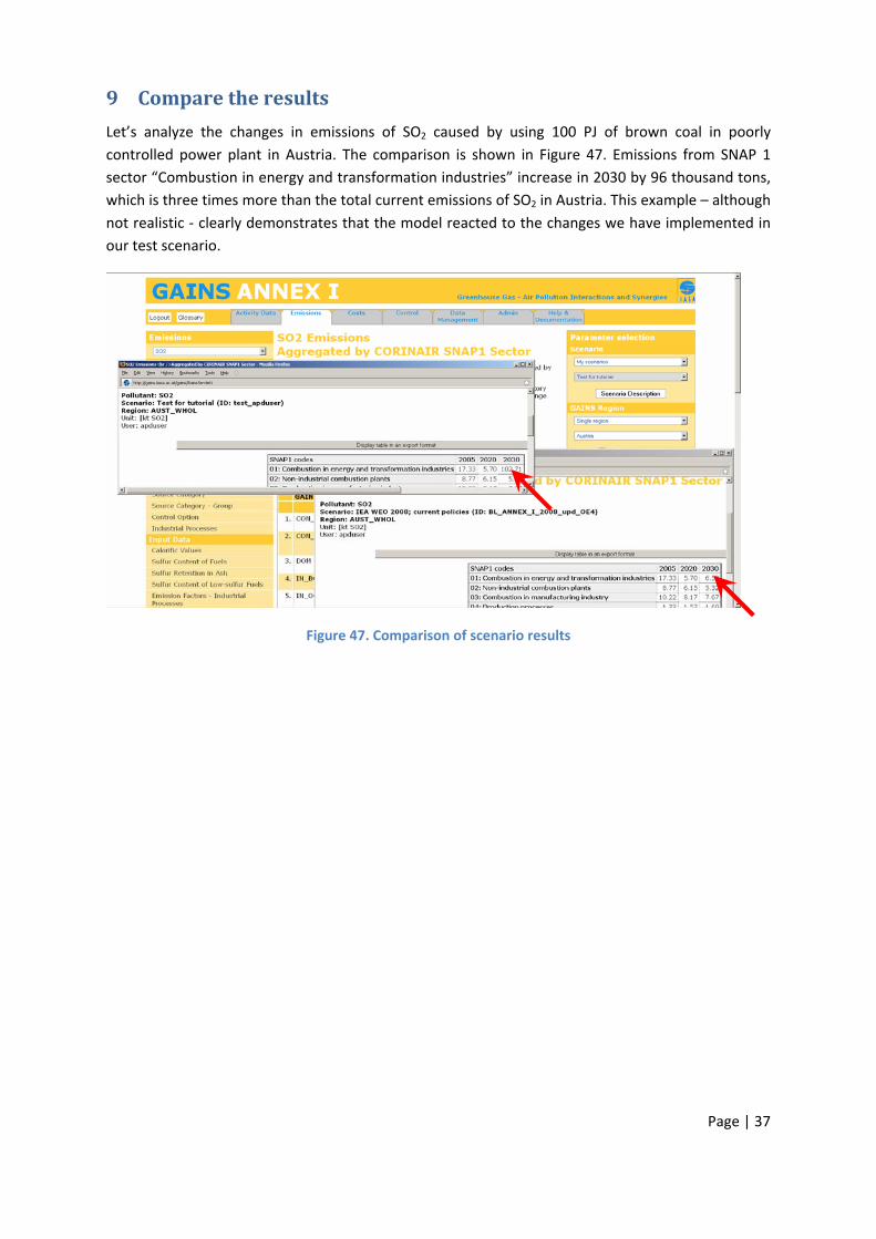
9 Compare the results
Let’s analyze the changes in emissions of SO2 caused by using 100 PJ of brown coal in poorly controlled power plant in Austria. The comparison is shown in Figure 47. Emissions from SNAP 1 sector “Combustion in energy and transformation industries” increase in 2030 by 96 thousand tons, which is three times more than the total current emissions of SO2 in Austria. This example – although not realistic ‐ clearly demonstrates that the model reacted to the changes we have implemented in our test scenario.
Figure 47. Comparison of scenario results
Page | 37
Page | 38
PART III Aggregation of energy data in GAINS
1 General
GAINS energy database includes three major components of energy system:
• Electricity and district heat generation in the power and district heating sector (PP)
• Energy use for primary fuel production, conversion of primary to secondary energy other than conversion to electricity and heat in the power and district heating plants, and for delivery of energy to final consumers (CON)
• Final energy use in: industry (IN), domestic sector (DOM), transport (TRA), and non‐energy use of fuels (NONEN). The domestic sector covers residential and commercial sectors, as well as agriculture, forestry, fishing and services.
Historic data have been extracted from energy statistics. GAINS contains alternative pathways of energy use up to 2030 derived from national and international energy projections, e.g., scenarios developed for Europe by the PRIMES model, projections of the International Energy Agency, scenarios based on national studies. While these data are stored in the GAINS database, they are exogenous input to GAINS.
Format of energy data in GAINS is convenient for calculating emissions of air pollutants and greenhouse gases. Energy tables show fuels that are actually used in combustion processes in various economic sectors. Fuel production figures, like coal mining or oil and gas extraction, are reported in process data tables only if they are relevant for emissions calculations. Also, crude oil input to refineries and coal input to coke plants do not appear in GAINS energy tables. Instead, products (outputs) from refineries and coke plants are shown as fuel consumption in energy consuming sectors. Again, crude oil input to refineries can be found in process activity data.
Total energy consumption in a given country can be derived by summing up the fuel use in the conversion sector (CON), power sector (PP) and final demand sectors i.e., IN, DOM, TRA, and NONEN. Although this total is a sum of primary and secondary energy, it is equal to the total primary energy demand at a country level.
Conversion of fuel consumption from natural units (tons, m3) should be made using net (or lower) calorific value of fuels.
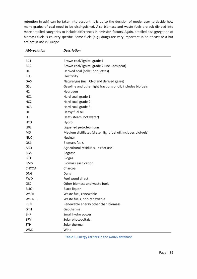
1.1 Aggregation of energy carriers GAINS includes a rather detailed specification of energy carriers. This is because emission factors for air pollutants and greenhouse gases heavily depend on a type and quality of fuel used. Consumption of fuel in a given economic sector determines the level of energy‐related activity used in emissions calculations.
List of energy carriers is shown in Table 1. For brown coal/lignite and hard coal different grades are distinguished. In this way differences in fuel quality (calorific value, sulfur and ash content, sulfur
Page | 39
retention in ash) can be taken into account. It is up to the decision of model user to decide how many grades of coal need to be distinguished. Also biomass and waste fuels are sub‐divided into more detailed categories to include differences in emission factors. Again, detailed disaggregation of biomass fuels is country‐specific. Some fuels (e.g., dung) are very important in Southeast Asia but are not in use in Europe.
Abbreviation Description
BC1 Brown coal/lignite, grade 1 BC2 Brown coal/lignite, grade 2 (includes peat) DC Derived coal (coke, briquettes) ELE Electricity GAS Natural gas (incl. CNG and derived gases) GSL Gasoline and other light fractions of oil; includes biofuels H2 Hydrogen HC1 Hard coal, grade 1 HC2 Hard coal, grade 2 HC3 Hard coal, grade 3 HF Heavy fuel oil HT Heat (steam, hot water) HYD Hydro LPG Liquefied petroleum gas MD Medium distillates (diesel, light fuel oil; includes biofuels) NUC Nuclear OS1 Biomass fuels ARD Agricultural residuals ‐ direct use BGS Bagasse BIO Biogas BMG Biomass gasification CHCOA Charcoal DNG Dung FWD Fuel wood direct OS2 Other biomass and waste fuels BLIQ Black liquor WSFR Waste fuel, renewable WSFNR Waste fuels, non‐renewable REN Renewable energy other than biomass GTH Geothermal SHP Small hydro power SPV Solar photovoltaic STH Solar thermal WND Wind
Table 1. Energy carriers in the GAINS database
Page | 40
In order to consider effects of switching to clean energy sources, GAINS also stores information on energy carriers that do not emit air pollutants, e.g., electricity, heat, renewables other than biomass.
1.2 Power plant sector (PP)
Power and district heating plants (PP_TOTAL) are the overarching sector that is subdivided into existing plants with wet bottom boilers (PP_EX_WB), other existing plants (PP_EX_OTH), IGCC plants (PP_IGCC), and other new plants (PP_NEW). Existing plants are defined as all capacities put into operation on or before December 31, 1995. Industrial power and CHP plants as well as public district heating plants are included here.
The power plant sector covers fuel inputs to‐ and gross electricity and heat output from power and district heating plants. It contains public power and district heating plants, power plants of auto‐producers, as well as public and industrial combined heat and power (CHP) plants. Fuel input is reported with a positive sign (+) and gross electricity and heat output is reported with a negative sign (‐). Losses and on‐site energy consumption are accounted for under the conversion sector (CON)
GAINS employs the "Total Primary Energy Supply" (TPES) convention for quantifying the primary energy equivalent of electricity generation from non‐fossil fuels. The TPES convention assumes 100% conversion efficiency for wind, solar, hydro and other non‐combustion renewable energy technologies. For geothermal power generation 10% conversion efficiency is assumed and 33% conversion efficiency is assumed for nuclear power plants.
1.3 Energy production and conversion/transformation sector (CON) The definition of the "conversion sector" (CON) in GAINS follows the "energy transformation sector" as defined in the energy balances of the International Energy Agency (www.iea.org). However, fuel input to‐ and (gross) electricity and heat output from the power and district heating plants is reported in the power sector. CON sector includes on‐site consumption of fuel and energy in coal mines, refineries, coke and briquette plants, gasification plants etc. It also includes own use of electricity and heat in the power and district heating sector, as well as transmission and distribution losses for electricity, heat, and gas
Sector CON is further divided into fuel used in combustion processes (CON_COMB) and own use and losses that occur without combustion (CON_LOSS). This distinction is necessary to account for different emission factors in combustion and non‐combustion part.
GAINS treats separately fuel combustion in boilers and in furnaces. This is because operating conditions, emission factors, and emission control technologies for these two types of combustors are different.
Sector CON_COMB covers fuel combustion in furnaces used in the energy sector. Examples are: combustion in crude oil distillation furnaces and catalytic cracking installations in oil refineries, or coking gas use for heating coke batteries in coke plants. Fuel combusted in heat only boilers (in oil refineries, coke plants, coalmines, coal gasification plants etc.) should be reported in the sector
Page | 41
called “Combustion in industrial boilers” (IN_BO)5. If it is not possible to distinguish between combustion in boilers and combustion in furnaces, please report all fuel combustion in energy industries belonging to the CON sector under CON_COMB.
Sector CON_LOSS includes the following items:
• Losses of fuels, electricity and district heat in transmission and distribution to final consumer
• Own use of electricity and heat in the power sector, i.e., a difference between gross electricity/heat output and the energy supplied to the grid. It also includes electricity use in pumped storage hydro plants.
• Use of electricity, heat and fuels in other plants belonging to the energy sector (coalmines, oil refineries, coke plants, gasification and liquefaction plants etc.)
• Difference between total fuel inputs to‐ and outputs from the conversion processes.
The latter bullet includes:
• For coke plants a difference between input of coal and gross output of coke and coke oven gas. Fuel lost is coal (HC)
• For oil refineries a difference between crude oil and other feedstocks input and gross output of petroleum products (residual oil, gasoline, medium distillates, refinery gas, other). Since GAINS does not include crude oil in the energy balance, we assume that fuel lost is heavy fuel oil (HF)
• For biomass liquefaction and gasification plants the difference between biomass input and gross output of products (liquid fuels, biogas). Fuel lost is biomass.
It may happen that in energy statistics the inputs of crude oil and other feedstocks to oil refinery is lower than the sum of outputs. This is due to the difficulty in reporting complicated energy flows within the refinery and in particular flows between its energy and petrochemical part. In such a case, please assume that energy losses are zero.
1.4 Industry Energy consumption in industry is divided into combustion in (heat only) boilers (IN_BO), other industrial combustion (IN_OCTOT), and non‐energy use (NONEN).
Boiler fuel consumption is divided into consumption in: the conversion sector (IN_CON_BO), chemical industry (IN_CHEM_BO), pulp and paper industry (IN_PAP_BO) and in other industries (IN_OTH_BO). If detailed split by sub‐sectors is not known for a given energy pathway, total boiler fuel consumption should be reported under "IN_OTH_BO".
Other industrial combustion (IN_OC_TOT) is divided into: iron and steel (IN_ISTE_OC), chemical (IN_CHEM_OC), non‐ferrous metals (IN_NFME_OC), non‐metallic minerals (IN_NMMI_OC), paper, pulp, and printing (IN_PAP_OC) and other manufacturing industries (IN_OTH_OC). If detailed split by sub‐sectors is not known for a given energy pathway, total fuel consumption should be reported under "IN_OTH_OC".
5 Fuel use in energy sector’s CHP plants need to be reported in the power plant (PP) sector
Page | 42
In case a division of fuel consumption between boilers and other combustion is not known, total fuel consumption can be reported under “other industrial combustion”.
For "other industrial combustion", GAINS calculates emissions based on activity data reported under "IN_OC". This column is internally calculated by the GAINS model during data initialization by subtracting energy use reported for cement and lime production from the total energy use in industry (IN_OCTOT). Thereby, the model takes into account the high retention of the sulfur during cement and lime production and calculates emissions from these activities under "industrial process emissions". These measures are taken to avoid double counting of emissions.
1.5 Domestic sector Domestic sector in GAINS (DOM) includes the following sub‐sectors:
• residential (DOM_RES);
• commercial and public services (DOM_COM);
• other services, agriculture, forestry, fishing, and non‐specified sub‐sectors (DOM_OTH).
Fuel consumption by mobile sources in agriculture and fishing should be included in the transport sector energy demand. Since energy statistics incorporate these categories in the domestic (DOM) sector, appropriate corrections to statistical data need to be made.
If detailed split of domestic energy consumption is not known, total sector consumption can be reported under "DOM_OTH".
1.6 Transport and other mobile sources Transport and other mobile source sector (TRA) is divided into transportation by road (TRA_RD), other non‐road mobile sources (TRA_OT), and sources from the so‐called national sea traffic (TRA_OTS). The latter includes seagoing ships and fishing boats operating between the ports in the same country. Each of the major sectors is additionally divided into more detailed vehicle categories.
Road transport
Vehicles in road transport are divided into the following categories:
• Motorcycles, mopeds and cars with 2‐stroke engines (TRA_RD_LD2‐GSL)
• Motorcycles and mopeds with 4‐stroke engines (TRA_RD_M4‐GSL)
• Cars and small buses with 4‐stroke engines (TRA_RD_LD4C)
• Light commercial trucks with 4‐stroke engines (TRA_RD_LD4T)
• Heavy duty buses (TRA_RD_HDB)
• Heavy duty trucks (TRA_RD_HDT)
For each vehicle type GAINS needs information on total annual fuel consumption by fuel type (in PJ), total annual vehicle‐kilometers driven (Gveh‐km), and vehicle numbers (1000 vehicles). Fuel consumption, kilometers driven and vehicle numbers are closely related. Consistency of these three data sets needs to be carefully checked, so that for each vehicle category annual kilometers driven per vehicle and average fuel consumption (in l fuel/100 km) are within realistic range and
Page | 43
correspond to policies in a given scenario.
Other mobile sources
Non‐road mobile sources (TRA_OT) are divided into the following categories:
• Vehicles and small machines with 2‐stroke engines (TRA_OT_LD2): loan movers, garden tools, hand held saws, motorboats, snow scooters etc.
• Mobile machines in construction and industry (TRA_OT_CNS). This fuel consumption is included in energy statistics under manufacturing industry. If this consumption is not known from national studies, GAINS assumes as a default that 100 percent of gasoline (GSL) and gasoil/diesel fuel (MD) used in the construction sector and 50 percent of industrial gasoil (MD) consumption in other manufacturing industry is used by mobile sources.
• Tractors and mobile machines in agriculture and forestry (TRA_OT_AGR). This fuel consumption is included in energy statistics under "agriculture and forestry". If this consumption is not known from national studies, GAINS assumes as a default that 80 percent of agricultural gasoil (MD) consumption is used by mobile sources.
• Inland waterways (TRA_OT_INW).
• Railways (TRA‐OT_RAI).
• Civil aviation (TRA_OT_AIR). Following methodology used in the IEA energy balances, total fuel consumption by air transport (domestic and international) is included. However, the emissions of air pollutants from that sector are calculated only for landing, taxi and take‐off cycles (LTO). CO2 emissions are calculated for domestic flights only (TRA_OT_AIR_DOM).
• National maritime shipping (TRA_OTS), i.e., movement of ships between ports in the same country and fishing vessels. The vessels are sub‐divided into large (>1000 GRT ‐ TRA_OTS_L) and medium (<1000 GRT ‐ TRA_OTS_M). National data do not include international marine bunkering. Emissions from international sea traffic are calculated outside GAINS.
• Other non‐road sources with 4‐stroke engines (TRA_OT_LB): small household and forestry machines military vehicles, motorboats; use of GAS by pipeline compressors is also included here.
For each vehicle type GAINS needs information on total annual fuel consumption by fuel type (in PJ), and vehicle numbers (1000 vehicles). Fuel consumption and vehicle numbers are closely related. Consistency of these two data sets needs to be carefully checked, so that for each vehicle category average fuel consumption (in l fuel per year) is within realistic range and corresponds to policies in a given scenario.