GALACTICS: Gaussian Sampling for Lattice-BasedConstant-Time Implementation of CryptographicSignatures, Revisited

GILLES BARTHE, MPI-SP and IMDEA Software Institute

SONIA BELAÏD, CryptoExpertsTHOMAS ESPITAU, Sorbonne Université, Laboratoire d’informatique de Paris 6

PIERRE-ALAIN FOUQUE, Université de RennesMÉLISSA ROSSI, Thales, ENS Paris, CNRS, PSL University, INRIA

MEHDI TIBOUCHI, NTT Corporation

In this paper, we propose a constant-time implementation of the BLISS lattice-based signature scheme. BLISS

is possibly the most efficient lattice-based signature scheme proposed so far, with a level of performance on

par with widely used pre-quantum primitives like ECDSA. It is only one of the few postquantum signatures to

have seen real-world deployment, as part of the strongSwan VPN software suite.

The outstanding performance of the BLISS signature scheme stems in large part from its reliance on

discrete Gaussian distributions, which allow for better parameters and security reductions. However, that

advantage has also proved to be its Achilles’ heel, as discrete Gaussians pose serious challenges in terms

of secure implementations. Implementations of BLISS so far have included secret-dependent branches and

memory accesses, both as part of the discrete Gaussian sampling and of the essential rejection sampling step

in signature generation. These defects have led to multiple devastating timing attacks, and were a key reason

why BLISS was not submitted to the NIST postquantum standardization effort. In fact, almost all of the actual

candidates chose to stay away from Gaussians despite their efficiency advantage, due to the serious concerns

surrounding implementation security.

Moreover, naive countermeasures will often not cut it: we show that a reasonable-looking countermeasure

suggested in previous work to protect the BLISS rejection sampling can again be defeated using novel timing

attacks, in which the timing information is fed to phase retrieval machine learning algorithm in order to

achieve a full key recovery.

Fortunately, we also present careful implementation techniques that allow us to describe an implementation

of BLISS with complete timing attack protection, achieving the same level of efficiency as the original

unprotected code, without resorting on floating point arithmetic or platform-specific optimizations like AVX

intrinsics. These techniques, including a new approach to the polynomial approximation of transcendental

function, can also be applied to the masking of the BLISS signature scheme, and will hopefully make more

efficient and secure implementations of lattice-based cryptography possible going forward.

Additional Key Words and Phrases: Timing Attack; Phase Retrieval algorithms; Constant-

time Implementation; Lattice-based Cryptography; Masking Countermeasure

INTRODUCTIONThe looming threat of general-purpose quantum computers against legacy public-key crypto-

graphic schemes makes it a pressing problem to prepare the concrete transition to postquantum

cryptgraphy. Lattice-based cryptography, in particular, offers an attractive alternative to currently

deployed schemes based e.g. on RSA and elliptic curves, thanks to strong theoretical security guar-

antees, a large array of achievable primitives, and a level of efficiency that can rival pre-quantum

constructions.

Despite their attractive theoretical properties, however, lattice-based constructions present novel

challenges in terms of implementation security, particularly with respect to side-channel attacks.

Taking signatures as an example, possibly the most efficient construction proposed so far is the

BLISS signature scheme of Ducas et al. [16], which features excellent performance and has seen

1

real-world deployment via the VPN software suite strongSwan. Later implementations of BLISS

show good hardware performance as well [34]. However, existing implementations of BLISS suffer

from significant leakage through timing side-channels, which have led to several devastating attacks

against the scheme [6, 9, 22, 33, 40]. The main feature of BLISS exploited in these attacks in the use

of discrete Gaussian distributions, either as part of the Gaussian sampling used to generate the

random nonces in BLISS signatures, or as part of the crucial rejection sampling step that forms the

core of the Fiat–Shamir with aborts framework that supports BLISS’s security.

Generally speaking, Gaussian distributions are ubiquitous in theoretical works on lattice-based

cryptography, thanks to their convenient behavior with respect to proofs of security and parameter

choices. However, their role in practical implementations is less clear, largely because of the

concerns surrounding implementation attacks. For example, BLISS was not submitted to the

NIST postquantum standardization effort due to those concerns, and second round candidate

Dilithium [18], which can be seen as a direct successor of BLISS, replaces Gaussian distributions

by uniform ones, at the cost of larger parameters and a less efficient implementation, specifically

citing implementation issues as their justification.

In this paper we study the security of the BLISS implementation against cache-based timing

and power side-channel attacks. Specifically, we develop efficient implementations of BLISS that

are secure against these attacks. Although our results target BLISS in particular, our techniques

can be applied to the very large class of constructions based on discrete Gaussian distributions (at

least those that use Gaussians with fixed standard deviation), which form the bulk of works on

lattice-based cryptography. Protecting implementations for these constructions are challenging

because state-of-the-art techniques for constant-time and masked implementations mainly consider

deterministic programs (and thus in particular for programs with deterministic control-flow).

However, schemes that involve Gaussian sampling. In particular, signature schemes within the

Fiat–Shamir with aborts framework use rejection sampling, also called the acceptance-rejection

method. To sample from a distribution X , with density f , one uses samples from the distribution Ywith density д as follows:

(1) Get a sample y from distribution Y and a sample u from the uniform distribution on (0, 1),(2) If u < f (y)/Mд(y), accept y as a sample drawn from X , and reject otherwise.

This algorithm requiresM iterations on average to obtain a sample and in particular does not have

deterministic control flow. A further difficulty with BLISS is that floating-point operations are gen-

erally not constant-time, and yet the computation of the function f (y)/д(y) involves transcendentalfunctions. It is thus an additional difficulty to implement it purely in terms of integer arithmetic.

Our Contributions. First of all, we present a new timing attack against a countermeasure pre-

viously suggested in [22] which avoids some earlier attacks [6, 22]. Previous attacks target the

Bernoulli sampling algorithm, while we look at the implementation of the hyperbolic cosine func-

tion. We show that the computation of this transcendental function leaks secret information and

that by measuring the number of times this algorithm restarts, we can recover the secret key. The

available information is similar to the one used in the phase retrieval problem, given |⟨a, s⟩| forknown and random samples a, recover s. The general phase retrieval problem [10] is that ⟨a, s⟩ canbe a complex value and we only get the amplitude and not the phase of this value. In the particular

case of this problem, where the scalar product is real, we devise 2 new efficient algorithms. The

first attack only uses the samples that the scalar product is null, which is not too restrictive here

since we have many such samples and performs a Principal Component Analysis algorithm. The

second attack takes into account all the information by using maximum likelihood estimator for

combining the correlation between many samples and perform a gradient descent. The difficulties

in our algorithms come from the truncation at the end of BLISS, to make the signature compact,

2

that introduces a lot of noise in our samples. Finally, both attacks rely on a clever use of lattice

reduction algorithm to recover all the secret information even though some errors are still present

at the end of the descent.

Then, we propose a constant-time implementation of BLISS, mainly relying on an alternate

implementation of the rejection sampling step, carried out by computing a sufficiently precise

polynomial approximation of the rejection probability using pure integer arithmetic. We manage

to do so using a novel technique for polynomial approximation, relying on lattice reduction for the

Euclidean inner product derived from the Sobolev norm. This approach has several advantageous

properties compared to methods based on minimax computations, as implemented e.g. in the Sollya

software package [11], especially in terms of its control on the shape of polynomial approximants

we can obtain. Our constant-time implementation, written in portable C using pure division-free

integer arithmetic, achieves the same level of efficiency as the original, variable-time implementation

of BLISS, and outperforms Dilithium by a large margin. We also provide experimental validation

using the dudect tool of Reparaz et al. that the implementation is indeed constant-time.

Using similar techniques, together with a proof strategy analogous to [3], we also show how to

construct a masked implementation of BLISS secure against high-order side-channel attacks.

Related Work. Several works have exhibited side-channel attacks against BLISS [6, 9, 22, 33].

These attacks epitomize the difficulties to implement lattice-based schemes securely, particularly

when Gaussians are involved. However, there are also positive results showing that it is possible to

make this signature scheme secure against such attacks. For instance, Barthe et al. [3] propose a

secure implementation against side-channel attack for the GLP signature [23]. This implementation

is made secure using the classical masking countermeasure used to prevent SPA and DPA analysis.

The security proof uses the strong non-interference property introduced in [2], which allows to

reason compositionally, and a relaxation of masking called masking under public outputs. However,

the masked implementation and security proof of GLP relies critically on the fact that samplings

are drawn from uniform distributions as Dilithium.

There exist a number of works devoted to constant-time techniques for sampling according to

discrete Gaussian distributions [20, 28, 32] or related distributions, such as rounded Gaussians [26].

There are different methods according to the size of the standard deviation, as well as whether it is

constant or varies: encryption scheme typically require small standard deviations, while signatures

use larger ones, which are fixed for Fiat–Shamir schemes and vary for hash-and-sign constructions.

To deal with large standard deviations, it is customary to use a small standard deviation “base

sampler” and build upon it to achieve the desired standard deviation: this is the approach presented

in [32]. These works can also be distinguished according as whether they require floating point

arithmetic. In particular, the rounded Gaussians of [26] offer numerous attractive properties, but

they have some statistical limitations in terms of distinguishing advantage, and they rely on floating

point implementations.

Approximating the exponential function with polynomials has been recently proposed in imple-

mentations of Gaussian sampling algorithms. Here, we apply this technique for the transcendental

functions used in the rejection sampling part of the signing algorithm. Prest was the first to propose

such ideas in [35] and he showed that with 53-bit of precision for floating numbers we can have

256-bit security when the number of signatures is limited to 264, as is stated in the requirements of

the NIST standardization process. NIST second round candidate Falcon [36] is based on a Gauss-

ian sampler that uses Padé approximants to evaluate the exponential function of the rejection

probability. More recently, Zhao et al. have proposed a polynomial approximation without float-

ing point division [43], since that operation is known to not be constant-time. They use floating

point multiplications instead to compute the exponential, but this instruction does not always

3

have constant-time execution guarantees either, unfortunately. In this paper, we approximate the

exponential and the hyperbolic cosine functions over an interval using integer polynomials to avoid

floating operations. Moreover, we aim to approximate using polynomials with small coefficients

so that we can use small-sized integers and obtain a straightforward implementation of Horner’s

algorithm.

Organisation of the paper. In Section 1, we recall the BLISS signature scheme and the implemen-

tation of the rejection sampling algorithm. Then, we describe our timing attacks on the hyperbolic

cosine implementation in Section 2. In Section 3, we present our constant-time implementation

of the BLISS signature scheme. Section 4 presents the technique we used to approximate tran-

scendental functions with integral polynomials. Our masked implementation is introduced in the

Appendix A.

1 DESCRIPTION OF THE BLISS SCHEMENotations. For any integer q, the ring Zq is represented by the integers in [−q/2,q/2) ∩ Z. Vectorsare considered as column vectors and will be written in bold lower case letters and matrices with

upper case letters. By default, we will use the L2 Euclidean norm, ∥v∥2 = (∑

i v2

i )1/2

and L∞-normas ∥v∥∞ = maxi |vi |. The notation ⌊x⌉d denotes the centered d highest-order significant bits of x :x = ⌊x⌉d · 2

d + x ′ with x ′ ∈ [−2d−1, 2d−1).

Overall description of BLISS. The BLISS signature scheme [16] is possibly the most efficient

lattice-based signature scheme so far. It has been implemented in both software [16] and hard-

ware [34]. BLISS can be seen as a ring-based optimization of the earlier lattice-based scheme of

Lyubashevsky [31], sharing the same “Fiat–Shamir with aborts” structure [30].

One can give a simplified description of the scheme as follows: the public key is an NTRU-like

ratio of the form aq = s2/s1 mod q, where the signing key polynomials s1, s2 ∈ R = Z[X ]/(Xn + 1)

are small and sparse. See Figure 1 for a description of the key generation. κ,C,δ1,δ2,q,p are

parameters detailed in BLISS specifications and Nκ is the function depicted in Equation 3.2.4. To

sign a message µ, one first generates commitment values y1, y2 ∈ R with normally distributed

coefficients (distribution denoted D ), and then computes a hash c of the message µ together

with u = −aqy1 + y2 mod q using a cryptographic hash function modeled as a random oracle

taking values in the set of elements of R with exactly κ coefficients equal to 1 and the others to

0. The signature is then the triple (c, z1, z2), with zi = yi + sic, and there is rejection sampling to

ensure that the distribution of zi is independent of the secret key. Verification is possible because

u = −aqz1 + z2 mod q.The real BLISS signature procedure, described in Figure 2, includes several optimizations on

top of the above description. In particular, to improve the repetition rate, it targets a bimodal

Gaussian distribution for the zi ’s, so there is a random sign flip in their definition. In addition, to

reduce signature size, the signature element z2 is actually transmitted in compressed form z†2, and

accordingly the hash input includes only a compressed version of u.The verification procedure is given in Figure 3 for completeness since it does not manipulate

sensitive data. B1 and B2 are parameters detailed in BLISS specifications.

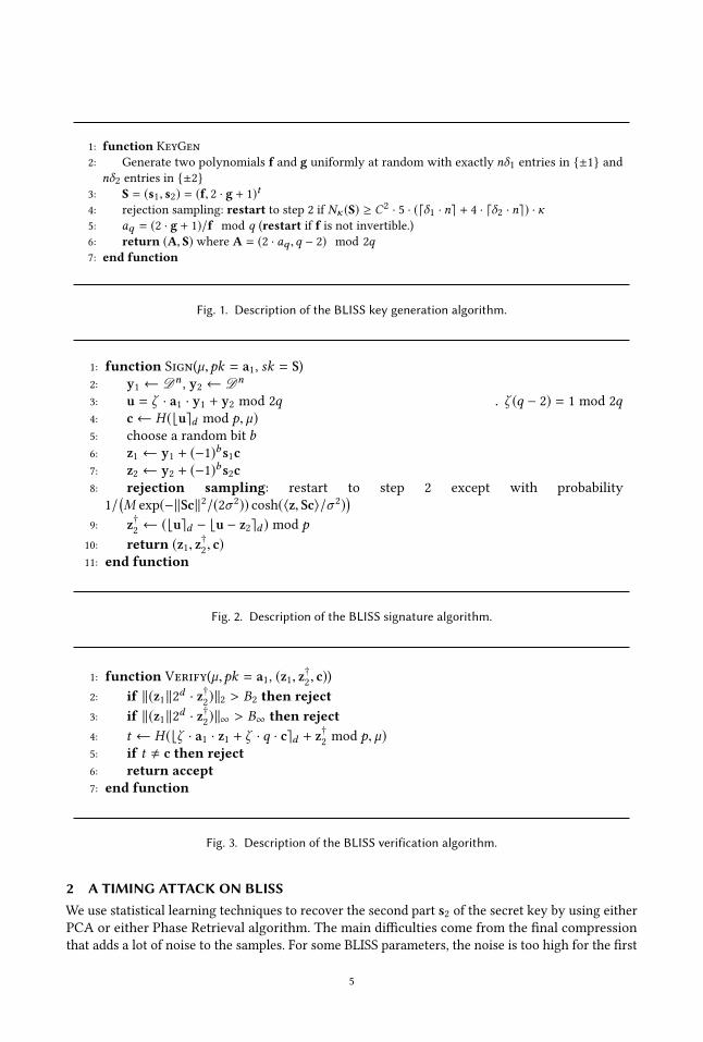
The original BLISS paper describes a family of concrete parameters for the signature scheme,

recalled in Table 1. The BLISS–I and BLISS–II parameter sets are optimized for speed and compact-

ness respectively, and both target 128 bits of security. BLISS–III and BLISS–IV are claimed to offer

160 and 192 bits of security respectively. Finally, a BLISS–0 variant is also given as a toy exemple

offering a relatively low security level.

4

1: function KeyGen

2: Generate two polynomials f and g uniformly at random with exactly nδ1 entries in {±1} andnδ2 entries in {±2}

3: S = (s1, s2) = (f, 2 · g + 1)t

4: rejection sampling: restart to step 2 if Nκ (S) ≥ C2 · 5 · (⌈δ1 · n⌉ + 4 · ⌈δ2 · n⌉) · κ5: aq = (2 · g + 1)/f mod q (restart if f is not invertible.)6: return (A, S) where A = (2 · aq ,q − 2) mod 2q7: end function

Fig. 1. Description of the BLISS key generation algorithm.

1: function Sign(µ,pk = a1, sk = S)2: y1 ← Dn

, y2 ← Dn

3: u = ζ · a1 · y1 + y2 mod 2q ▷ ζ (q − 2) = 1 mod 2q4: c← H (⌊u⌉d mod p, µ)5: choose a random bit b6: z1 ← y1 + (−1)bs1c7: z2 ← y2 + (−1)bs2c8: rejection sampling: restart to step 2 except with probability

1/(M exp(−∥Sc∥2/(2σ 2)) cosh(⟨z, Sc⟩/σ 2)

)9: z†

2← (⌊u⌉d − ⌊u − z2⌉d ) mod p

10: return (z1, z†2, c)

11: end function

Fig. 2. Description of the BLISS signature algorithm.

1: function Verify(µ,pk = a1, (z1, z†2, c))

2: if ∥(z1∥2d · z†2)∥2 > B2 then reject

3: if ∥(z1∥2d · z†2)∥∞ > B∞ then reject

4: t ← H (⌊ζ · a1 · z1 + ζ · q · c⌉d + z†2mod p, µ)

5: if t , c then reject6: return accept7: end function

Fig. 3. Description of the BLISS verification algorithm.

2 A TIMING ATTACK ON BLISSWe use statistical learning techniques to recover the second part s2 of the secret key by using either

PCA or either Phase Retrieval algorithm. The main difficulties come from the final compression

that adds a lot of noise to the samples. For some BLISS parameters, the noise is too high for the first

5

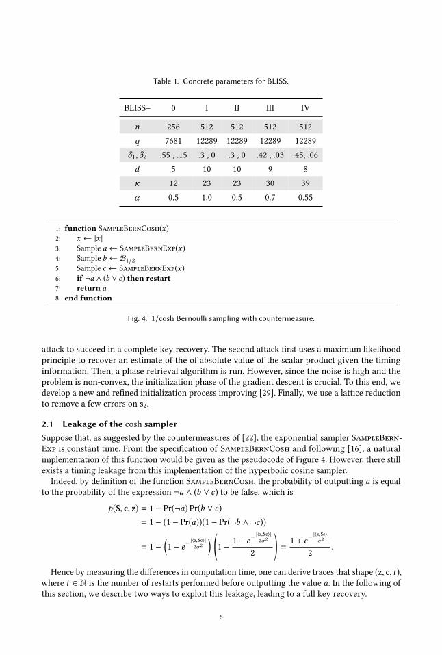
Table 1. Concrete parameters for BLISS.

BLISS– 0 I II III IV

n 256 512 512 512 512

q 7681 12289 12289 12289 12289

δ1,δ2 .55 , .15 .3 , 0 .3 , 0 .42 , .03 .45, .06

d 5 10 10 9 8

κ 12 23 23 30 39

α 0.5 1.0 0.5 0.7 0.55

1: function SampleBernCosh(x )2: x ← |x |3: Sample a ← SampleBernExp(x)4: Sample b ← B

1/2

5: Sample c ← SampleBernExp(x)6: if ¬a ∧ (b ∨ c) then restart7: return a8: end function

Fig. 4. 1/cosh Bernoulli sampling with countermeasure.

attack to succeed in a complete key recovery. The second attack first uses a maximum likelihood

principle to recover an estimate of the of absolute value of the scalar product given the timing

information. Then, a phase retrieval algorithm is run. However, since the noise is high and the

problem is non-convex, the initialization phase of the gradient descent is crucial. To this end, we

develop a new and refined initialization process improving [29]. Finally, we use a lattice reduction

to remove a few errors on s2.

2.1 Leakage of the cosh samplerSuppose that, as suggested by the countermeasures of [22], the exponential sampler SampleBern-

Exp is constant time. From the specification of SampleBernCosh and following [16], a natural

implementation of this function would be given as the pseudocode of Figure 4. However, there still

exists a timing leakage from this implementation of the hyperbolic cosine sampler.

Indeed, by definition of the function SampleBernCosh, the probability of outputting a is equal

to the probability of the expression ¬a ∧ (b ∨ c) to be false, which is

p(S, c, z) = 1 − Pr(¬a) Pr(b ∨ c)

= 1 − (1 − Pr(a))(1 − Pr(¬b ∧ ¬c))

= 1 −

(1 − e−

|⟨z,Sc⟩|2σ 2

) (1 −

1 − e−|⟨z,Sc⟩|2σ 2

2

)=

1 + e−|⟨z,Sc⟩|σ 2

2

.

Hence by measuring the differences in computation time, one can derive traces that shape (z, c, t),where t ∈ N is the number of restarts performed before outputting the value a. In the following of

this section, we describe two ways to exploit this leakage, leading to a full key recovery.

6

1: Collectm traces (zi, ci, ti )2: for i = 0 tom do3: if ti = 0 thenW ← ciz∗i · ciz

∗iT end if

4: end for5: S←

$N(0, 1)n ; S← S

∥s0 ∥6: for i = 0 to K then7: S←W −1S; S← S

∥s0 ∥8: end for9: return round(

S∥S∥N )

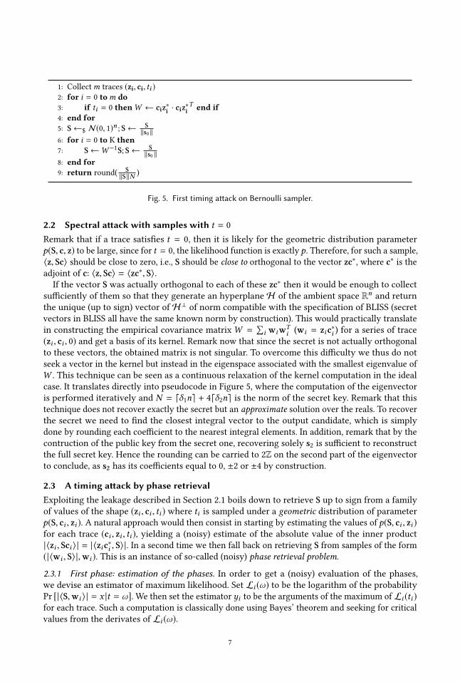
Fig. 5. First timing attack on Bernoulli sampler.

2.2 Spectral attack with samples with t = 0

Remark that if a trace satisfies t = 0, then it is likely for the geometric distribution parameter

p(S, c, z) to be large, since for t = 0, the likelihood function is exactly p. Therefore, for such a sample,

⟨z, Sc⟩ should be close to zero, i.e., S should be close to orthogonal to the vector zc∗, where c∗ is theadjoint of c: ⟨z, Sc⟩ = ⟨zc∗, S⟩.If the vector S was actually orthogonal to each of these zc∗ then it would be enough to collect

sufficiently of them so that they generate an hyperplaneH of the ambient space Rn and return

the unique (up to sign) vector ofH⊥ of norm compatible with the specification of BLISS (secret

vectors in BLISS all have the same known norm by construction). This would practically translate

in constructing the empirical covariance matrixW =∑

i wiwTi (wi = zic∗i ) for a series of trace

(zi , ci , 0) and get a basis of its kernel. Remark now that since the secret is not actually orthogonal

to these vectors, the obtained matrix is not singular. To overcome this difficulty we thus do not

seek a vector in the kernel but instead in the eigenspace associated with the smallest eigenvalue of

W . This technique can be seen as a continuous relaxation of the kernel computation in the ideal

case. It translates directly into pseudocode in Figure 5, where the computation of the eigenvector

is performed iteratively and N = ⌈δ1n⌉ + 4⌈δ2n⌉ is the norm of the secret key. Remark that this

technique does not recover exactly the secret but an approximate solution over the reals. To recover

the secret we need to find the closest integral vector to the output candidate, which is simply

done by rounding each coefficient to the nearest integral elements. In addition, remark that by the

contruction of the public key from the secret one, recovering solely s2 is sufficient to reconstruct

the full secret key. Hence the rounding can be carried to 2Z on the second part of the eigenvector

to conclude, as s2 has its coefficients equal to 0, ±2 or ±4 by construction.

2.3 A timing attack by phase retrievalExploiting the leakage described in Section 2.1 boils down to retrieve S up to sign from a family

of values of the shape (zi , ci , ti ) where ti is sampled under a geometric distribution of parameter

p(S, ci , zi ). A natural approach would then consist in starting by estimating the values of p(S, ci , zi )for each trace (ci , zi , ti ), yielding a (noisy) estimate of the absolute value of the inner product

|⟨zi , Sci ⟩| = |⟨zic∗i , S⟩|. In a second time we then fall back on retrieving S from samples of the form

(|⟨wi , S⟩|,wi ). This is an instance of so-called (noisy) phase retrieval problem.

2.3.1 First phase: estimation of the phases. In order to get a (noisy) evaluation of the phases,

we devise an estimator of maximum likelihood. Set Li (ω) to be the logarithm of the probability

Pr [|⟨S,wi ⟩| = x |t = ω]. We then set the estimator yi to be the arguments of the maximum of Li (ti )for each trace. Such a computation is classically done using Bayes’ theorem and seeking for critical

values from the derivates of Li (ω).

7

1: A← [w1 | · · · |wm ]

2: s0 ←$N(0, 1)n

3: for i = 0 to K then4: s0 ← AT diag(y1, . . . ,ym )As05: s0 ← (ATA)−1s06: s0 ←

s0∥s0 ∥

7: end for8: s0 ←

s0∥s0 ∥

N

9: return rounding(s0)

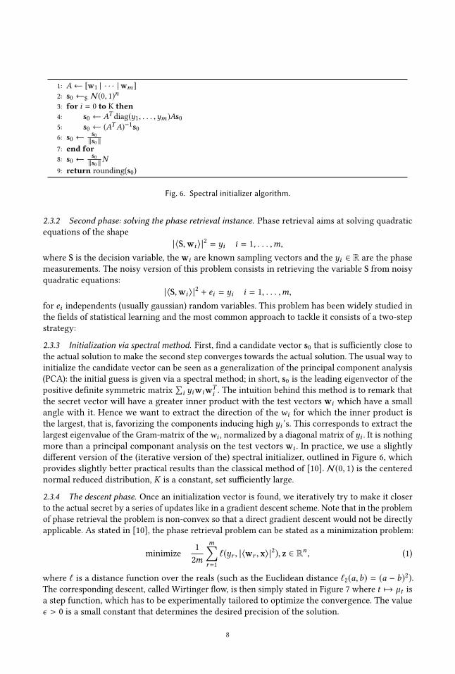
Fig. 6. Spectral initializer algorithm.

2.3.2 Second phase: solving the phase retrieval instance. Phase retrieval aims at solving quadratic

equations of the shape

|⟨S,wi ⟩|2 = yi i = 1, . . . ,m,

where S is the decision variable, the wi are known sampling vectors and the yi ∈ R are the phase

measurements. The noisy version of this problem consists in retrieving the variable S from noisy

quadratic equations:

|⟨S,wi ⟩|2 + ei = yi i = 1, . . . ,m,

for ei independents (usually gaussian) random variables. This problem has been widely studied in

the fields of statistical learning and the most common approach to tackle it consists of a two-step

strategy:

2.3.3 Initialization via spectral method. First, find a candidate vector s0 that is sufficiently close to

the actual solution to make the second step converges towards the actual solution. The usual way to

initialize the candidate vector can be seen as a generalization of the principal component analysis

(PCA): the initial guess is given via a spectral method; in short, s0 is the leading eigenvector of the

positive definite symmetric matrix

∑i yiwiwT

i . The intuition behind this method is to remark that

the secret vector will have a greater inner product with the test vectors wi which have a small

angle with it. Hence we want to extract the direction of the wi for which the inner product is

the largest, that is, favorizing the components inducing high yi ’s. This corresponds to extract the

largest eigenvalue of the Gram-matrix of thewi , normalized by a diagonal matrix of yi . It is nothingmore than a principal componant analysis on the test vectors wi . In practice, we use a slightly

different version of the (iterative version of the) spectral initializer, outlined in Figure 6, which

provides slightly better practical results than the classical method of [10]. N(0, 1) is the centerednormal reduced distribution, K is a constant, set sufficiently large.

2.3.4 The descent phase. Once an initialization vector is found, we iteratively try to make it closer

to the actual secret by a series of updates like in a gradient descent scheme. Note that in the problem

of phase retrieval the problem is non-convex so that a direct gradient descent would not be directly

applicable. As stated in [10], the phase retrieval problem can be stated as a minimization problem:

minimize

1

2m

m∑r=1

ℓ(yr , |⟨wr , x⟩|2), z ∈ Rn , (1)

where ℓ is a distance function over the reals (such as the Euclidean distance ℓ2(a,b) = (a − b)2).

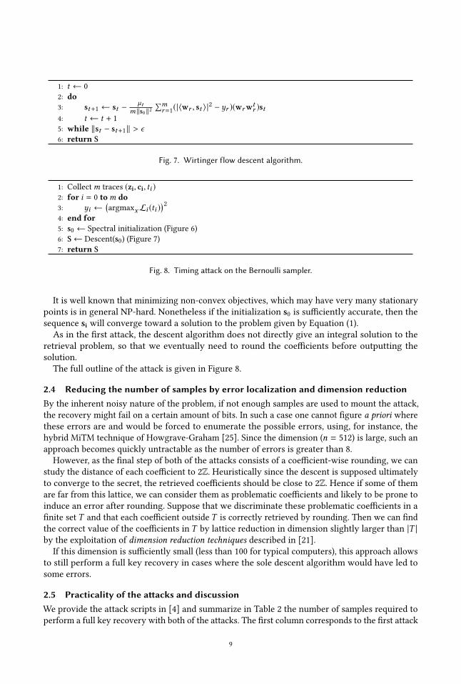
The corresponding descent, called Wirtinger flow, is then simply stated in Figure 7 where t 7→ µt isa step function, which has to be experimentally tailored to optimize the convergence. The value

ϵ > 0 is a small constant that determines the desired precision of the solution.

8

1: t ← 0

2: do3: st+1 ← st −

µtm ∥s0 ∥2

∑mr=1(|⟨wr , st ⟩|2 − yr )(wrwt

r )st4: t ← t + 15: while ∥st − st+1∥ > ϵ6: return S

Fig. 7. Wirtinger flow descent algorithm.

1: Collectm traces (zi, ci, ti )2: for i = 0 tom do3: yi ←

(argmaxxLi (ti )

)2

4: end for5: s0 ← Spectral initialization (Figure 6)

6: S← Descent(s0) (Figure 7)7: return S

Fig. 8. Timing attack on the Bernoulli sampler.

It is well known that minimizing non-convex objectives, which may have very many stationary

points is in general NP-hard. Nonetheless if the initialization s0 is sufficiently accurate, then the

sequence si will converge toward a solution to the problem given by Equation (1).

As in the first attack, the descent algorithm does not directly give an integral solution to the

retrieval problem, so that we eventually need to round the coefficients before outputting the

solution.

The full outline of the attack is given in Figure 8.

2.4 Reducing the number of samples by error localization and dimension reductionBy the inherent noisy nature of the problem, if not enough samples are used to mount the attack,

the recovery might fail on a certain amount of bits. In such a case one cannot figure a priori where

these errors are and would be forced to enumerate the possible errors, using, for instance, the

hybrid MiTM technique of Howgrave-Graham [25]. Since the dimension (n = 512) is large, such an

approach becomes quickly untractable as the number of errors is greater than 8.

However, as the final step of both of the attacks consists of a coefficient-wise rounding, we can

study the distance of each coefficient to 2Z. Heuristically since the descent is supposed ultimately

to converge to the secret, the retrieved coefficients should be close to 2Z. Hence if some of them

are far from this lattice, we can consider them as problematic coefficients and likely to be prone to

induce an error after rounding. Suppose that we discriminate these problematic coefficients in a

finite set T and that each coefficient outside T is correctly retrieved by rounding. Then we can find

the correct value of the coefficients in T by lattice reduction in dimension slightly larger than |T |by the exploitation of dimension reduction techniques described in [21].

If this dimension is sufficiently small (less than 100 for typical computers), this approach allows

to still perform a full key recovery in cases where the sole descent algorithm would have led to

some errors.

2.5 Practicality of the attacks and discussionWe provide the attack scripts in [4] and summarize in Table 2 the number of samples required to

perform a full key recovery with both of the attacks. The first column corresponds to the first attack

9

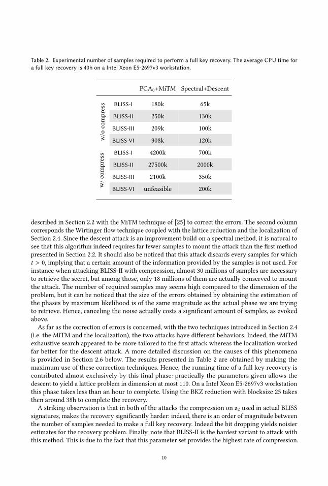
Table 2. Experimental number of samples required to perform a full key recovery. The average CPU time fora full key recovery is 40h on a Intel Xeon E5-2697v3 workstation.

PCA0+MiTM Spectral+Descent

BLISS-I 180k 65k

BLISS-II 250k 130k

BLISS-III 209k 100k

BLISS-VI 308k 120k

w/ocompress

BLISS-I 4200k 700k

BLISS-II 27500k 2000k

BLISS-III 2100k 350k

BLISS-VI unfeasible 200k

w/compress

described in Section 2.2 with the MiTM technique of [25] to correct the errors. The second column

corresponds the Wirtinger flow technique coupled with the lattice reduction and the localization of

Section 2.4. Since the descent attack is an improvement build on a spectral method, it is natural to

see that this algorithm indeed requires far fewer samples to mount the attack than the first method

presented in Section 2.2. It should also be noticed that this attack discards every samples for which

t > 0, implying that a certain amount of the information provided by the samples is not used. For

instance when attacking BLISS-II with compression, almost 30 millions of samples are necessary

to retrieve the secret, but among those, only 18 millions of them are actually conserved to mount

the attack. The number of required samples may seems high compared to the dimension of the

problem, but it can be noticed that the size of the errors obtained by obtaining the estimation of

the phases by maximum likelihood is of the same magnitude as the actual phase we are trying

to retrieve. Hence, canceling the noise actually costs a significant amount of samples, as evoked

above.

As far as the correction of errors is concerned, with the two techniques introduced in Section 2.4

(i.e. the MiTM and the localization), the two attacks have different behaviors. Indeed, the MiTM

exhaustive search appeared to be more tailored to the first attack whereas the localization worked

far better for the descent attack. A more detailed discussion on the causes of this phenomena

is provided in Section 2.6 below. The results presented in Table 2 are obtained by making the

maximum use of these correction techniques. Hence, the running time of a full key recovery is

contributed almost exclusively by this final phase: practically the parameters given allows the

descent to yield a lattice problem in dimension at most 110. On a Intel Xeon E5-2697v3 workstation

this phase takes less than an hour to complete. Using the BKZ reduction with blocksize 25 takes

then around 38h to complete the recovery.

A striking observation is that in both of the attacks the compression on z2 used in actual BLISS

signatures, makes the recovery significantly harder: indeed, there is an order of magnitude between

the number of samples needed to make a full key recovery. Indeed the bit dropping yields noisier

estimates for the recovery problem. Finally, note that BLISS-II is the hardest variant to attack with

this method. This is due to the fact that this parameter set provides the highest rate of compression.

10

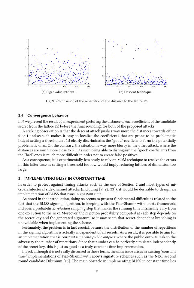
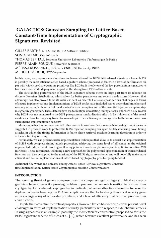
(a) Eigenvalue retrieval (b) Descent technique

Fig. 9. Comparison of the repartition of the distance to the lattice 2Z.

2.6 Convergence behaviorIn 9 we present the result of an experiment picturing the distance of each coefficient of the candidate

secret from the lattice 2Z before the final rounding, for both of the proposed attacks.

A striking observation is that the descent attack pushes way more the distances towards either

0 or 1 and as such makes it easy to localize the coefficients that are prone to be problematic.

Indeed setting a threshold at 0.5 clearly discriminates the “good” coefficients form the potentially

problematic ones. On the contrary, the situation is way more blurry in the other attack, where the

distances are much more close to 0.5. As such being able to distinguish the “good” coefficients from

the “bad” ones is much more difficult in order not to create false positives.

As a consequence, it is experimentally less costly to rely on MitM technique to resolve the errors

in this latter case as setting a threshold too low would imply reducing lattices of dimension too

large.

3 IMPLEMENTING BLISS IN CONSTANT TIMEIn order to protect against timing attacks such as the one of Section 2 and most types of mi-

croarchitectural side-channel attacks (including [9, 22, 33]), it would be desirable to design an

implementation of BLISS that runs in constant time.

As noted in the introduction, doing so seems to present fundamental difficulties related to the

fact that the BLISS signing algorithm, in keeping with the Fiat–Shamir with aborts framework,

includes a probabilistic rejection sampling step that makes the running time intrisically vary from

one execution to the next. Moreover, the rejection probability computed at each step depends on

the secret key and the generated signature, so it may seem that secret-dependent branching is

unavoidable when implementing the scheme.

Fortunately, the problem is in fact crucial, because the distribution of the number of repetitions

in the signing algorithm is actually independent of all secrets. As a result, it is possible to aim for

an implementation that is constant time with public outputs, where the public outputs leak to the

adversary the number of repetitions. Since that number can be perfectly simulated independently

of the secret key, this is just as good as a truly constant time implementation.

In fact, although it is not really discussed in those terms, the same issue arises in existing “constant

time” implementations of Fiat–Shamir with aborts signature schemes such as the NIST second

round candidate Dilithium [18]. The main obstacle in implementing BLISS in constant time lies

11

elsewhere, in what forms the key difference between those two lattice-based schemes: BLISS’s

reliance on discrete Gaussian distributions, whereas Dilithium only uses uniform distributions,

with the explicit goal of avoiding side-channel vulnerabilities in the implementation.

The use of Gaussian distributions leads to two main implementation challenges: the constant

time implementation of Gaussian sampling, and that of the rejection sampling, corresponding to

Step 2 and Step 8 of Figure 2. In addition, some care must be taken regarding the implementation

of the ring-valued hash function from Step 4, as well as the sign flips in Steps 6 and 7. We describe

our implementation choices below and provide further technical details at the end of this section.

We note that most of these implementation techniques would apply equally well to other

Fiat–Shamir signatures schemes using Gaussian distributions, and in particular to the optimized

variant BLISS–B [15]. Regarding BLISS–B, the only subtle point is the computation of Sc, whichnow involves sign flips and can no longer be carried out using an NTT; it is still easy if c is

considered non-sensitive (which is reasonable but requires additional assumptions), but becomes

significantly more expensive otherwise. We also note that our approach supports arbitrary Gaussian

standard deviations, which could in principle allow for more efficient parameter settings; to make

comparisons more meaningful, we did not attempt to select new parameters, but this could be

interesting further work.

3.1 Overview of our constant-time implementationThe main design goal of our implementation is to obtain a fast, constant-time implementation of

BLISS (focusing on the BLISS–I parameter set, which offers the best trade-off between security

and efficiency) while maintaining a high degree of portability. With the latter goal in mind, we

choose to rely entirely on integer arithmetic (limited to additions, multiplications and shifts on

32-bit and 64-bit operands). Indeed, division instructions and floating point operations rarely offer

constant-time execution guarantees,1and they can present serious security challenges related to

weak determinism [17].

The ingredients needed to implement the signing algorithm are as follows: we need Gaussian

sampling for Step 2 of Figure 2; ring multiplication for Steps 3, 6 and 7; ring-valued hashing for Step 4;

and rejection sampling for Step 8. Other operations like constant-time sign flips, ring additions and

signature compression are straightforward. We now give a description of our implemention choices

for each of these steps. Note that in terms of efficiency, the critical elements are the Gaussian

sampling and the ring multiplication, with the ring-valued hashing also taking up a significant

amount of time. The other operations take negligible time in comparison.

3.1.1 Gaussian sampling. The Gaussian sampling step is key to obtaining a fast implementation

of BLISS, as it represents half or more of the computation time of signature generation: for each

signature, one needs to generate 1024 samples of the discrete Gaussian distribution Dσ (possibly

several times over, in case a rejection occurs), and the standard deviation is relatively large (σ = 205

for BLISS–I). This step has also been specifically targeted by cache timing attacks such as [9].

Several approaches can be considered for implementing it in constant time, but they have wildly

different running times. All approaches first generate samples from the non-negative Gaussian D+σ ,and then use a random sign flip (in constant time) to recover the entire distribution.

The most naive way would be to rely on cumulative distribution table (CDT) sampling: pre-

compute a table of the cumulative distribution function of D+σ covering the inverval at the points

1Regarding floating point arithmetic, it is often variable time even in the presence of an FPU, and even for simpler operations

like multiplications. For example, the fmul multiplication instruction can have variable latency on several x86 architectures,

including the Intel Pentium III!

12

of which the distribution has a non-negligible probability2 ≳ 2

−128; then, to produce a sample,

generate a random value in [0, 1] with 128 bits of precision, and return the index of the first entry

in the table greater than that value. In variable time, this can be done relatively efficiently with

a binary search, but this leaks the resulting sample through memory access patterns. As a result,

a constant time implementation has essentially no choice but to read the entire table each time

and carry out each and every comparison. Although a basic CDT implementation would store the

cumulative probabilities with 128 bits of precision, it is in fact possible to only store lower precision

approximations, as discussed in [34, 41] (see also [35] for an alternate approach using “conditional

distribution functions”). Nevertheless, since the table should contain σ√2λ log 2 ≈ 2730 entries

for BLISS–I, we are looking at 22 kB’s worth of memory access for every generated sample. The

resulting implementation is obviously highly inefficient. Other table-based approaches like the

Knuth-Yao algorithm similarly suffer from constant time constraints.

A more efficient approach, originally introduced by Pöppelmann et al. [34] and later improved

and generalized by Micciancio and Walter [32], assumes that we can generate a base Gaussian

distribution D+σ0 with not too small standard deviation σ0, and allows to then combine samples

from that base distribution to achieve larger standard deviations. For the parameters of BLISS–I,

one can check that the optimal choice is to let σ 2

0= σ 2

(92+72)(32+22). One can then generate a sample

x statistically close to D+σ from 4 samples x0,0,x0,1,x1,0,x1,1 from D+σ0 , as x = 9x0 + 7x1, wherexi = 3xi,0 + 2xi,1. Since σ0 ≈ 4.99 is much smaller than σ , using a CDT approach for the base

sampler is more reasonable: the CDT table now stores 63 entries. Generating a sample requires

reading through the table 4 times, for a total of 2 kB of memory access and 128 bits of randomness

per sample. It turns out, however, that the performance of the resulting implementation in our

setting is still somewhat underwhelming.

The authors of the qTesla3second round NIST submission [1] proposed an ingenious approach

to improve constant-time CDT-based discrete Gaussian sampling. In practice, one needs to generate

many samples from the discrete Gaussian distribution in each signature (one for each coefficient

of the yi polynomials). The idea is then to batch all of the searches through the CDT table corre-

sponding to those samples. This can be done in constant time by applying an oblivious sorting

algorithm (e.g. network sorting) to the concatenation of the CDT with the list of uniform random

samples. This can be used in conjunction with the convolution technique of [32, 34] in order to

reduce the total size of the table to be sorted (which is the sum of the CDT size and of the desired

number of samples). Preliminary attempts to use this approach in the case of BLISS did not result

in compelling performance numbers, but there is likely room for improvement in terms of the

oblivious sorting algorithm involved as well as the way is algorithm is combined with various

optimization tricks: detailed investigation of this question is left as interesting further work.

Finally, yet another strategy is to generate a discrete Gaussian of very small standard deviation,

use it to construct a distribution that looks somewhat like D+σ but is not statistically close, and

use rejection sampling to correct the discrepancy. This is actually the approach taken in the

original BLISS paper [16]. Concretely, what that paper essentially does is sample some x from the

distribution D+σ2 where σ2 = σ/k , and some y uniform in {0, . . . ,k − 1}. Then, z = kx + y looks

“somewhat like” a sample from D+σ , and one can check that rejecting z except with probability

exp

(−y(y + 2kx)/(2σ 2)

)yields a value that actually follows D+σ . As observed in the BLISS paper,

this rejection sampling step is exactly of the same form as the one used for the overall signing

algorithm. The constant time implementation of that step is described in Section 3.1.4 below, and

we can simply reuse that work to obtain our Gaussian sampling. The only ingredient to add is

2Even taking Rényi divergence arguments into account, values taken with probability ≥ 2

−117should included.

3While qTesla uses uniform randomness during signature generation, it does use discrete Gaussians for key generation.

13

a base sampler for the distribution D+σ2 , since the one in the original BLISS paper does not lend

itself to a convenient constant time implementation. Fortunately, choosing k = 256, the standard

deviation σ2 ≈ 0.80 is really small, and hence a CDT approach only requires 10 table entries. In

practice, this yields a Gaussian sampling of very reasonable efficiency, whose cost is dominated

by the cost of the rejection sampling step, and of the generation of the uniform randomness. This

is the approach we choose for our implementation. Its security directly follows from that of the

rejection sampling (see Section 4 for technical details).

3.1.2 Ring multiplications. As usual in ideal lattice-based schemes, ring multiplications such as

the one in Step 3 of Figure 2 are carried out using the number-theoretic transform (NTT). Since the

NTT does not use any secret-dependent conditional branches or memory accesses, constant-time

implementation does not pose any particular difficulty. In our case, we directly adapt the NTT from

the reference implementation of Dilithium, which uses the bit-reversed order for coefficients in the

NTT domain, lazy modular reductions, and the Montgomery representation for values modulo q.Only a few simple changes are needed compared to Dilithium, in order to account for the different

modulus q = 12289 and the higher degree n = 512 (instead of q = 8380417 and n = 256 respectively).

At the cost of more frequent modular reductions, we could do the entire computation on 16-bit

integers (which could yield to faster automatic vectorization), but for simplicity, we keep the 32-bit

arithmetic from the Dilithium NTT.

The implementation choice for the ring multiplications in Steps 6 and 7 of Figure 2 is less obvious.

Indeed, those steps involve the multiplication of the secret key elements, which are small, by the

hash value c, which has 23 coefficients equal to 1, and the others equal to 0. Moreover, we can

show that, under a non-standard but reasonable LWE-like assumption, BLISS remains secure even

when u and hence c are made public (including for rejected instances). It would therefore not

jeopardize security to implement the multiplications s1c and s2c as repeated additions of shifted

versions of s1 and s2, where the memory access patterns in the shifts reveal the coefficients of c (butnothing about the secret key vectors themselves). Interestingly, however, it turns out that, at least

on our target platform, implementing the multiplications that way is not faster than using the NTT,

probably because the NTT has a much better cache locality. As a result, all ring multiplications in

our implementation simply use the NTT.

3.1.3 Ring-valued hashing. Step 4 of the signing algorithm in Figure 2 computes the “challenge”

ring element c = H (⌊u⌉d mod q, µ) from the “commitment” u and the input message µ. That ringelement should be a polynomial uniformly sampled among those with κ = 23 coefficients equal to

1, and all other coefficients equal to 0. To construct such a polynomial, we first pass the inputs of Hto an extendable output function (XOF), in our case SHAKE128, and then use the resulting random

stream to sample the list (i1, . . . , iκ ) of indices in c equal to 1.

Concretely speaking, we again follow Dilithium’s approach, which proceeds as follows. We pick

i1 uniformly in {0, . . . ,n −κ}. Then i2 is chosen uniformly in {0, . . . ,n −κ + 1}, and if it happens tocollide with i1, it is set to n−κ+1 instead. Continuing, ik is chosen uniformly in {0, . . . ,n−κ−1+k},and replaced by n − κ − 1 + k if it coincides with one of the previous values. It is easy to check that

{i1, . . . , iκ } is then a uniformly distributed κ-element subset of {0, . . . ,n − 1} as required.However, Dilithium’s implementation of this strategy is not in fact constant-time, as it works

by updating an n-element array and modifying the elements at indices ik and n − κ − 1 + k for

each k . As a result, the algorithm leaks the entirety of c through memory accesses. This is not a

critical problem, since as we have mentioned, the values u and hence c are not really sensitive in

BLISS (security is still achieved for the variant in which those values are revealed, albeit under

a less standard hardness assumption: this is exactly analogous to how the security of the r-GLPscheme from [3] is proved under the non-standard r-DCK assumption).

14

Nevertheless, in order to avoid relying on additional assumptions compared to the original BLISS

paper, we opt for a completely constant time implementation of the same approach instead. Our

idea is to add ik to the list of previously obtained indices using a constant-time insertion sort, and

do a constant-time swap between ik and n − κ − 1 + k in case a collision occurs. In principle, that

approach has quadratic complexity in κ, but since κ is so small, the overhead is negligible: we

find that our constant-time approach is only a few thousand cycles slower than the variable time

algorithm (about 1–2% of the entire running time of signature generation).

3.1.4 Rejection sampling. Finally, the last step we need to implement in constant time is the

rejection sampling. In other words, at the end of the signature generation algorithm, we need to

sample bits bexp and b1/cosh that take the value 1 with probability

pexp = exp

(−K − ∥Sc∥2

2σ 2

)and p1/cosh = 1/cosh

(⟨z, Sc⟩σ 2

)respectively (where K is a known constant).

To do so, the approach taken in the original BLISS paper relies on iterated Bernoulli trials with

known constant probabilities for bexp, and recursively calls this exponential sampling algorithm to

sample b1/cosh. Again, the variable time nature of these algorithms has led to multiple attacks.

As mentioned in [22], it is relatively easy to modify the function SampleBernExp from Figure 4

to run in constant time: simply carry out every iteration every time, and accumulate the results of

the Bernoulli trials using constant time logic expressions. However, the performance penalty of

doing so is significant, due to the lack of early aborts. This is not a serious problem for the rejection

sampling step itself, since it is only carried out a handful of times per signature. However, since

this exponential rejection sampling function is also called as part of Gaussian sampling (as we

recall from Section 3.1.1 above), any slow down will strongly affect the running time of the entire

signature generation. Moreover, while the bexp part can be made constant time, doing so is much

harder for b1/cosh, as we have discussed in Section 2.

An alternate approach is to simply evaluate the values pexp and p1/cosh with sufficient precision,

and compare them to uniform random values in [0, 1]. The challenge is to do so in constant time,

using only integer arithmetic. In particular, we cannot rely on floating point implementations of

transcendental functions like exp and cosh.

The approach we take is to replace the exp function by a sufficiently close polynomial approxi-

mation, and similarly for cosh. Then, pexp can be evaluated in fixed point to sufficient precision

using an application of Horner’s algorithm, entirely with integer arithmetic; and 1/p1/cosh can be

evaluated using the same code by expressing cosh in terms of exp. There are several steps involved

in carrying out that strategy:

(1) determine the precisionwe need to ensure security. To do so, we use amethodology introduced

by Prest [35] based on the Rényi divergence. It shows that 45 bits of relative precision suffice

for security, provided that the number of generated signatures is at most 264(as specified in

the NIST competition).

(2) compute a polynomial approximation on the required interval of the function f : x 7→exp

(x/(2σ 2)

), achieving the relative precision we need. To do so, we introduce a novel

technique based on lattice reduction for the Sobolev Euclidean norm on polynomials. This

technique lets us precisely control the shape of the polynomial we get, in order to ensure

that Horner’s algorithm can be applied without any overflow using 64-bit integer arithmetic.

Compared to earlier techniques such as the L∞ approximations of Brisebarre and Chevil-

lard [8], it also has the advantage of eliminating heuristics (since a bound on the Sobolev

norm directly yields a bound on the functional ∥ · ∥∞ norm), and of avoiding the computation

15

Table 3. Performance results and comparison (kcycles).

LQ Median UQ Const. time?

Dilithium (ref) 286 515 1526 !

Dilithium (avx2) 142 332 428 !

qTesla-I (ref) 243 418 781 %

Original BLISS 188 194 313 %

Our implementation 218 220 223 !

of minimax polynomials (since the closest polynomial in the Sobolev norm can be obtained

using a simple Euclidean projection).

(3) extend the range of that polynomial approximation in order to support the larger interval

required for the cosh computation (as well as for the rejection step in Gaussian sampling).

This is done by computing a constant c such that f (c) is very close to 2, so that f (k · c + x) =f (c)k · f (x) can be easily obtained from f (x) using small multiplications and shifts.

(4) deduce an algorithm for the cosh part of the rejection sampling. The nontrivial point here is

that we end up evaluating a good approximation of p ′ = 1/p1/cosh. Testing if u < p1/cosh, forsome u ∈ [0, 1], reduces to testing if u · p ′ < 1. The multiplication involves numbers with

over 45 bits of precision, however, so the result does not fit within 64 bits, and thus requires

some degree of bit fiddling. Intermediate conditional branches also need to be written in

constant time.

Full technical details regarding these various steps are provided in Section 4 below.

The idea of using polynomial approximations to evaluate pexp already appears in earlier work: as

part of the FACCT Gaussian sampler described in [43]. In particular, our own Gaussian sampler

can be seen as a variant of FACCT. There are multiple differences between our works, however:

in particular, FACCT relies on floating point arithmetic, which we specifically seek to avoid,4and

uses off-the-shelf software to obtain a double precision floating point polynomial approximation of

the function f . Moreover, since FACCT focuses on Gaussian sampling, that paper does not directly

address the cosh issue.

3.2 Security and performanceUsing the techniques described above, we wrote a constant-time implementation of BLISS in

portable C (specifically for the BLISS–I parameters), that can be found in [4]. We now provide

some data regarding its performance, and provide a short formal treatment of its security.

We point out that our code only implements signature generation in constant time. Obviously,

signature verification does not manipulate any secret, and hence does not need to be made constant

time; however, one may wish to ensure that key generation is constant time as well. We have not

attempted to do so, since key generation is carried out much less often and usually in much more

controlled conditions than actual signing. However, it is not difficult to modify our implementation

to make key generation constant time as well. The building blocks involved are briefly discussed at

the end of this section.

4We think the argument from [43] to the effect that floating point multiplications are constant time is overly optimistic.

As mentioned earlier, this is not true on some older x86 platforms, to say nothing of more exotic, more lightweight or

FPU-less architectures. Besides, as highlighted in [17], floating points arithmetic may lead to a vulnerbability called weak

determinism which can sometimes lead to complete breaks.

16

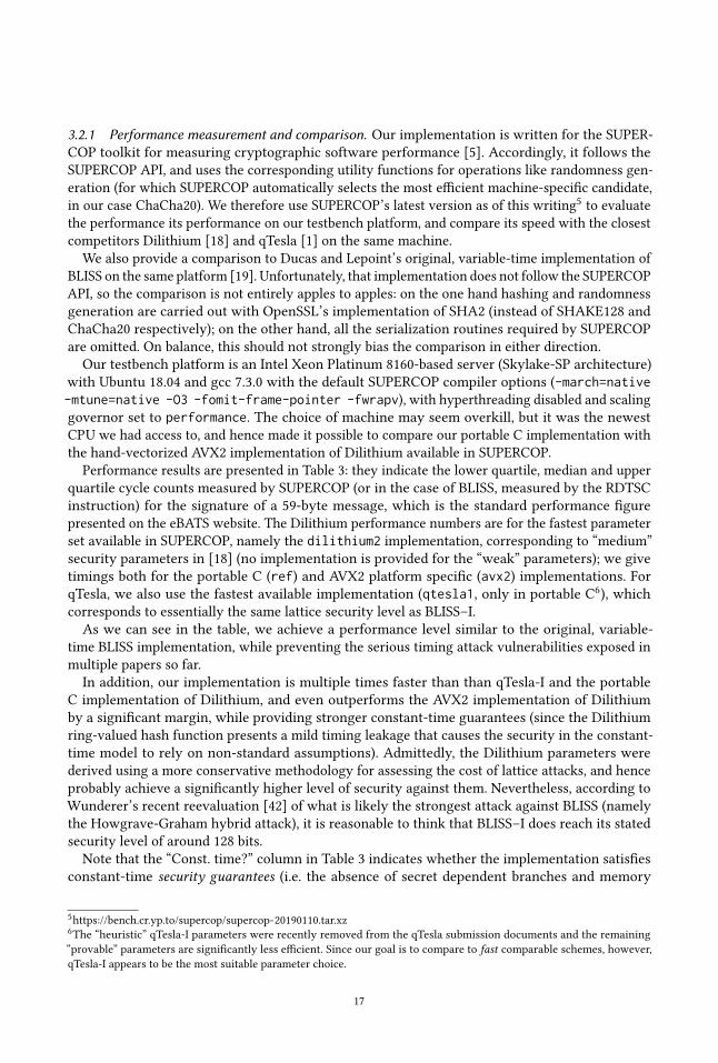
3.2.1 Performance measurement and comparison. Our implementation is written for the SUPER-

COP toolkit for measuring cryptographic software performance [5]. Accordingly, it follows the

SUPERCOP API, and uses the corresponding utility functions for operations like randomness gen-

eration (for which SUPERCOP automatically selects the most efficient machine-specific candidate,

in our case ChaCha20). We therefore use SUPERCOP’s latest version as of this writing5to evaluate

the performance its performance on our testbench platform, and compare its speed with the closest

competitors Dilithium [18] and qTesla [1] on the same machine.

We also provide a comparison to Ducas and Lepoint’s original, variable-time implementation of

BLISS on the same platform [19]. Unfortunately, that implementation does not follow the SUPERCOP

API, so the comparison is not entirely apples to apples: on the one hand hashing and randomness

generation are carried out with OpenSSL’s implementation of SHA2 (instead of SHAKE128 and

ChaCha20 respectively); on the other hand, all the serialization routines required by SUPERCOP

are omitted. On balance, this should not strongly bias the comparison in either direction.

Our testbench platform is an Intel Xeon Platinum 8160-based server (Skylake-SP architecture)

with Ubuntu 18.04 and gcc 7.3.0 with the default SUPERCOP compiler options (-march=native-mtune=native -O3 -fomit-frame-pointer -fwrapv), with hyperthreading disabled and scalinggovernor set to performance. The choice of machine may seem overkill, but it was the newest

CPU we had access to, and hence made it possible to compare our portable C implementation with

the hand-vectorized AVX2 implementation of Dilithium available in SUPERCOP.

Performance results are presented in Table 3: they indicate the lower quartile, median and upper

quartile cycle counts measured by SUPERCOP (or in the case of BLISS, measured by the RDTSC

instruction) for the signature of a 59-byte message, which is the standard performance figure

presented on the eBATS website. The Dilithium performance numbers are for the fastest parameter

set available in SUPERCOP, namely the dilithium2 implementation, corresponding to “medium”

security parameters in [18] (no implementation is provided for the “weak” parameters); we give

timings both for the portable C (ref) and AVX2 platform specific (avx2) implementations. For

qTesla, we also use the fastest available implementation (qtesla1, only in portable C6), which

corresponds to essentially the same lattice security level as BLISS–I.

As we can see in the table, we achieve a performance level similar to the original, variable-

time BLISS implementation, while preventing the serious timing attack vulnerabilities exposed in

multiple papers so far.

In addition, our implementation is multiple times faster than than qTesla-I and the portable

C implementation of Dilithium, and even outperforms the AVX2 implementation of Dilithium

by a significant margin, while providing stronger constant-time guarantees (since the Dilithium

ring-valued hash function presents a mild timing leakage that causes the security in the constant-

time model to rely on non-standard assumptions). Admittedly, the Dilithium parameters were

derived using a more conservative methodology for assessing the cost of lattice attacks, and hence

probably achieve a significantly higher level of security against them. Nevertheless, according to

Wunderer’s recent reevaluation [42] of what is likely the strongest attack against BLISS (namely

the Howgrave-Graham hybrid attack), it is reasonable to think that BLISS–I does reach its stated

security level of around 128 bits.

Note that the “Const. time?” column in Table 3 indicates whether the implementation satisfies

constant-time security guarantees (i.e. the absence of secret dependent branches and memory

5https://bench.cr.yp.to/supercop/supercop-20190110.tar.xz

6The “heuristic” qTesla-I parameters were recently removed from the qTesla submission documents and the remaining

“provable” parameters are significantly less efficient. Since our goal is to compare to fast comparable schemes, however,

qTesla-I appears to be the most suitable parameter choice.

17

0.0E+00 1.0E+06 2.0E+06 3.0E+06 4.0E+06 5.0E+060.32

1.00

3.16

10.00

31.62

100.00

GalacticsqTeslaOrig. BLISS

number of signatures

t-valu

e (log-s

cale

)

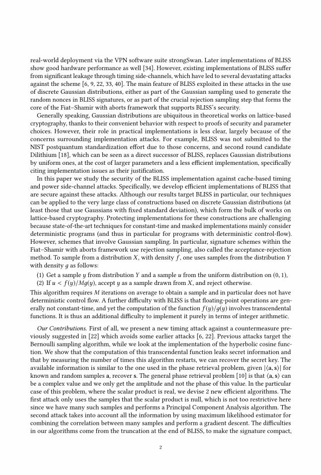
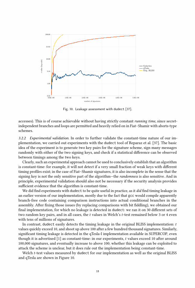
Fig. 10. Leakage assessment with dudect [37].

accesses). This is of course achievable without having strictly constant running time, since secret-

independent branches and loops are permitted and heavily relied on in Fiat–Shamir with aborts-type

schemes.

3.2.2 Experimental validation. In order to further validate the constant-time nature of our im-

plementation, we carried out experiments with the dudect tool of Reparaz et al. [37]. The basicidea of the experiment is to generate two key pairs for the signature scheme, sign many messages

randomly with either of the two signing keys, and check if a statistical difference can be observed

between timings among the two keys.

Clearly, such an experimental approach cannot be used to conclusively establish that an algorithm

is constant-time: for example, it will not detect if a very small fraction of weak keys with different

timing profiles exist; in the case of Fiat–Shamir signatures, it is also incomplete in the sense that the

signing key is not the only sensitive part of the algorithm—the randomness is also sensitive. And in

principle, experimental validation should also not be necessary if the security analysis provides

sufficient evidence that the algorithm is constant-time.

We did find experiments with dudect to be quite useful in practice, as it did find timing leakage in

an earlier version of our implementation, mostly due to the fact that gcc would compile apparently

branch-free code containing comparison instructions into actual conditional branches in the

assembly. After fixing those issues (by replacing comparisons with bit fiddling), we obtained our

final implementation, for which no leakage is detected in dudect: we ran it on 30 different sets of

two random key pairs, and in all cases, the t values in Welch’s t-test remained below 3 or 4 even

with tens of millions of signatures.

In contrast, dudect easily detects the timing leakage in the original BLISS implementation: tvalues quickly exceed 10, and shoot up above 100 after a few hundred thousand signatures. Similarly,

significant timing leakage is detected in the qTesla-I implementation available in SUPERCOP, even

though it is advertised [1] as constant-time: in our experiments, t values exceed 10 after around

100,000 signatures, and eventually increase to above 100; whether this leakage can be exploited to

attack the scheme is unclear, but it does rule out the implementation being constant-time.

Welch t-test values measured by dudect for our implementation as well as the original BLISS

and qTesla are shown in Figure 10.

18

Adversary Challenger

(KeyGen,Sign,Verify)←−−−−−−−−−−−−−−−−

pk

←−− (sk, pk) ← KeyGen(1λ)

q queries

µ (1)−−−→ (

σ (1),L (1)

Sign

)← ExecObs(Sign, µ(1), pk, sk)

σ (1), L(1)

Sign←−−−−−−−−...

µ (q)−−−→ (

σ (q),L(q)Sign

)← ExecObs(Sign, µ(q), pk, sk)

σ (q), L(q)Sign

←−−−−−−−−

forgery

{ µ∗, σ ∗−−−−−→

b ← Verify(pk, µ∗,σ ∗) ∧ (µ∗ < {µ(1), . . . , µ(q)})

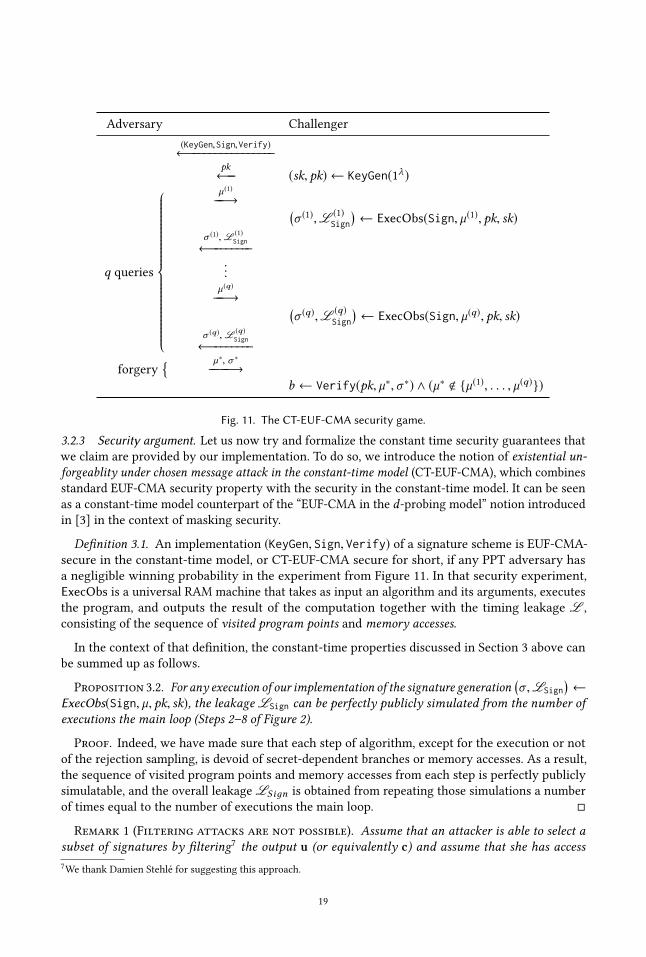
Fig. 11. The CT-EUF-CMA security game.

3.2.3 Security argument. Let us now try and formalize the constant time security guarantees that

we claim are provided by our implementation. To do so, we introduce the notion of existential un-

forgeablity under chosen message attack in the constant-time model (CT-EUF-CMA), which combines

standard EUF-CMA security property with the security in the constant-time model. It can be seen

as a constant-time model counterpart of the “EUF-CMA in the d-probing model” notion introduced

in [3] in the context of masking security.

Definition 3.1. An implementation (KeyGen, Sign, Verify) of a signature scheme is EUF-CMA-

secure in the constant-time model, or CT-EUF-CMA secure for short, if any PPT adversary has

a negligible winning probability in the experiment from Figure 11. In that security experiment,

ExecObs is a universal RAM machine that takes as input an algorithm and its arguments, executes

the program, and outputs the result of the computation together with the timing leakage L ,

consisting of the sequence of visited program points and memory accesses.

In the context of that definition, the constant-time properties discussed in Section 3 above can

be summed up as follows.

Proposition 3.2. For any execution of our implementation of the signature generation

(σ ,LSign

)←

ExecObs(Sign, µ, pk, sk), the leakage LSign can be perfectly publicly simulated from the number of

executions the main loop (Steps 2–8 of Figure 2).

Proof. Indeed, we have made sure that each step of algorithm, except for the execution or not

of the rejection sampling, is devoid of secret-dependent branches or memory accesses. As a result,

the sequence of visited program points and memory accesses from each step is perfectly publicly

simulatable, and the overall leakage LSiдn is obtained from repeating those simulations a number

of times equal to the number of executions the main loop. □

Remark 1 (Filtering attacks are not possible). Assume that an attacker is able to select a

subset of signatures by filtering7the output u (or equivalently c) and assume that she has access

7We thank Damien Stehlé for suggesting this approach.

19

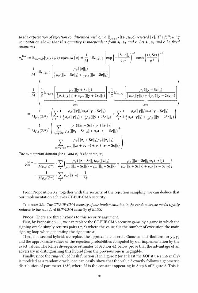
to the expectation of rejection conditionned with c, i.e. Ey1,y2,b [(z1, z2, c) rejected | c]. The followingcomputation shows that this quantity is independent from s1, s2 and c. Let s1, s2 and c be fixed

quantities,

pblisssc := Ey1,y2,b [(z1, z2, c) rejected | c] =1

M· Ey1,y2,b

[exp

(−∥S · c∥22σ 2

)−1cosh

(⟨z, Sc⟩σ 2

)−1]=

1

M· Ey1,y2,b

[ρσ (∥z∥2)

1

2ρσ (∥z − Sc∥2) + 1

2ρσ (∥z + Sc∥2)

]

=1

M·

©­­­­­­«1

2

Ey1,y2

[ρσ (∥y + Sc∥2)

1

2ρσ (∥y∥2) + 1

2ρσ (∥y + 2Sc∥2)

]︸ ︷︷ ︸

b=0

+1

2

Ey1,y2

[ρσ (∥y − Sc∥2)

1

2ρσ (∥y∥2) + 1

2ρσ (∥y − 2Sc∥2)

]︸ ︷︷ ︸

b=1

ª®®®®®®¬=

1

Mρσ (Zm)·

(∑y

1

2

ρσ (∥y∥2)ρσ (∥y + Sc∥2)1

2ρσ (∥y∥2) + 1

2ρσ (∥y + 2Sc∥2)

+∑y

1

2

ρσ (∥y∥2)ρσ (∥y − Sc∥2)1

2ρσ (∥y∥2) + 1

2ρσ (∥y − 2Sc∥2)

)=

1

Mρσ (Zm)·

( ∑z1=y+Sc

ρσ (∥z1 − Sc∥2)ρσ (∥z1∥2)ρσ (∥z1 − Sc∥2) + ρσ (∥z1 + Sc∥2)

+

∑z2=y−Sc

ρσ (∥z2 + Sc∥2)ρσ (∥z2∥2)ρσ (∥z2 + Sc∥2) + ρσ (∥z2 − Sc∥2)

).

The summation domain for z1 and z2 is the same, so,

pblisssc =1

Mρσ (Zm)·∑z

(ρσ (∥z − Sc∥2)ρσ (∥z∥2)

ρσ (∥z − Sc∥2) + ρσ (∥z + Sc∥2)+

ρσ (∥z + Sc∥2)ρσ (∥z∥2)ρσ (∥z + Sc∥2) + ρσ (∥z − Sc∥2)

)=

1

Mρσ (Zm)·∑zρσ (∥z∥2) =

1

M.

From Proposition 3.2, together with the security of the rejection sampling, we can deduce that

our implementation achieves CT-EUF-CMA security.

Theorem 3.3. The CT-EUF-CMA security of our implementation in the random oracle model tightly

reduces to the standard EUF-CMA security of BLISS.

Proof. There are three hybrids to this security argument.

First, by Proposition 3.2, we can replace the CT-EUF-CMA security game by a game in which the

signing oracle simply returns pairs (σ , ℓ) where the value ℓ is the number of execution the main

signing loop when generating the signature σ .Then, in a second hybrid, we replace the approximate discrete Gaussian distributions for y1, y2

and the approximate values of the rejection probabilities computed by our implementation by the

exact values. The Rényi divergence estimates of Section 4.1 below prove that the advantage of an

adversary in distinguishing this hybrid from the previous one is negligible.

Finally, since the ring-valued hash function H in Figure 2 (or at least the XOF it uses internally)

is modeled as a random oracle, one can easily show that the value ℓ exactly follows a geometric

distribution of parameter 1/M , where M is the constant appearing in Step 8 of Figure 2. This is

20

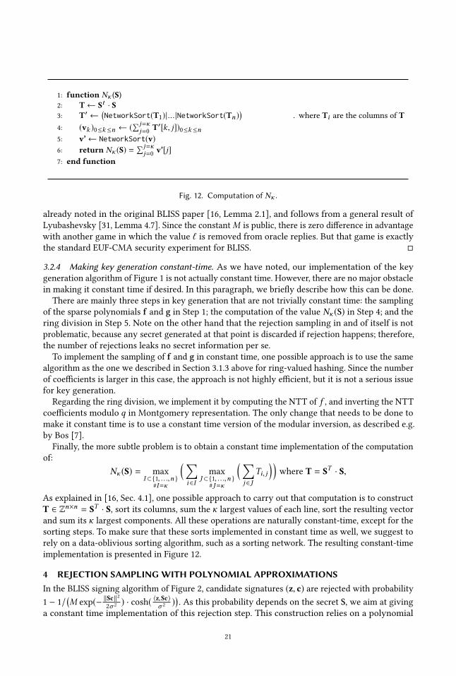
1: function Nκ (S)2: T← St · S3: T′ ←

(NetworkSort(T1)|...|NetworkSort(Tn )

)▷ where Ti are the columns of T

4: (vk )0≤k≤n ← (∑j=κj=0 T

′[k, j])0≤k≤n

5: v’← NetworkSort(v)6: return Nκ (S) =

∑j=κj=0 v’[j]

7: end function

Fig. 12. Computation of Nκ .

already noted in the original BLISS paper [16, Lemma 2.1], and follows from a general result of

Lyubashevsky [31, Lemma 4.7]. Since the constantM is public, there is zero difference in advantage

with another game in which the value ℓ is removed from oracle replies. But that game is exactly

the standard EUF-CMA security experiment for BLISS. □

3.2.4 Making key generation constant-time. As we have noted, our implementation of the key

generation algorithm of Figure 1 is not actually constant time. However, there are no major obstacle

in making it constant time if desired. In this paragraph, we briefly describe how this can be done.

There are mainly three steps in key generation that are not trivially constant time: the sampling

of the sparse polynomials f and g in Step 1; the computation of the value Nκ (S) in Step 4; and the

ring division in Step 5. Note on the other hand that the rejection sampling in and of itself is not

problematic, because any secret generated at that point is discarded if rejection happens; therefore,

the number of rejections leaks no secret information per se.

To implement the sampling of f and g in constant time, one possible approach is to use the same

algorithm as the one we described in Section 3.1.3 above for ring-valued hashing. Since the number

of coefficients is larger in this case, the approach is not highly efficient, but it is not a serious issue

for key generation.

Regarding the ring division, we implement it by computing the NTT of f , and inverting the NTTcoefficients modulo q in Montgomery representation. The only change that needs to be done to

make it constant time is to use a constant time version of the modular inversion, as described e.g.

by Bos [7].

Finally, the more subtle problem is to obtain a constant time implementation of the computation

of:

Nκ (S) = max

I ⊂{1, ...,n }#I=κ

(∑i ∈I

max

J ⊂{1, ...,n }#J=κ

(∑j ∈J

Ti, j))

where T = ST · S,

As explained in [16, Sec. 4.1], one possible approach to carry out that computation is to construct

T ∈ Zn×n = ST · S, sort its columns, sum the κ largest values of each line, sort the resulting vector

and sum its κ largest components. All these operations are naturally constant-time, except for the

sorting steps. To make sure that these sorts implemented in constant time as well, we suggest to

rely on a data-oblivious sorting algorithm, such as a sorting network. The resulting constant-time

implementation is presented in Figure 12.

4 REJECTION SAMPLINGWITH POLYNOMIAL APPROXIMATIONSIn the BLISS signing algorithm of Figure 2, candidate signatures (z, c) are rejected with probability

1 − 1/(M exp(−

∥Sc∥22σ 2) · cosh(

⟨z,Sc⟩σ 2)). As this probability depends on the secret S, we aim at giving

a constant time implementation of this rejection step. This construction relies on a polynomial

21

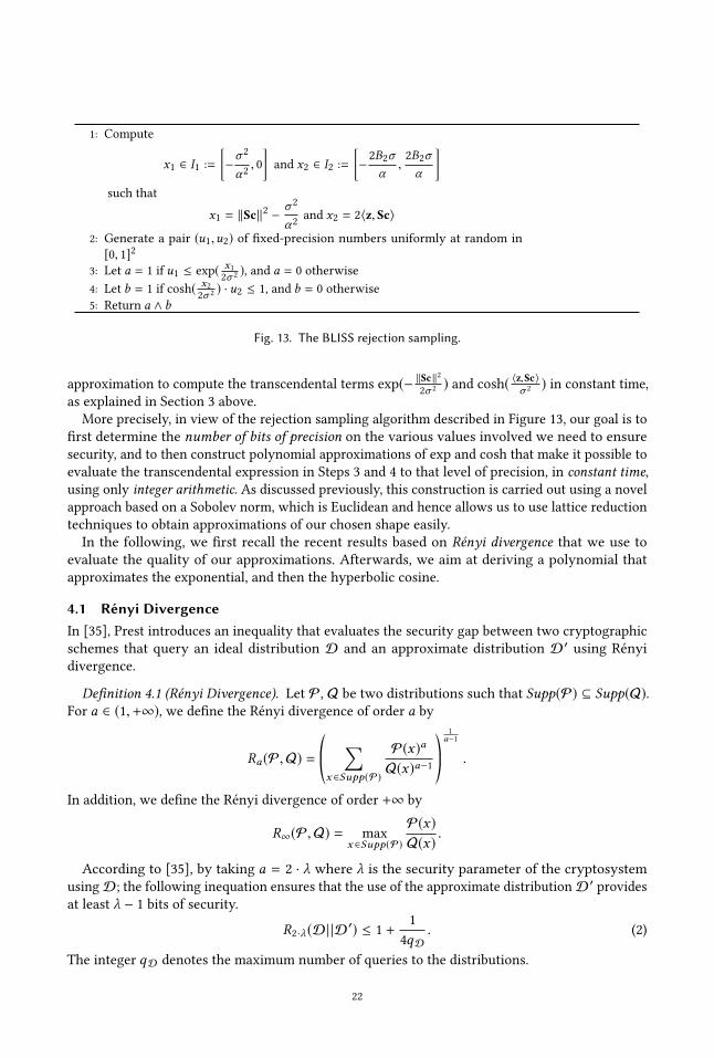
1: Compute

x1 ∈ I1 :=

[−σ 2

α2, 0

]and x2 ∈ I2 :=

[−2B2σ

α,2B2σ

α

]such that

x1 = ∥Sc∥2 −σ 2

α2and x2 = 2⟨z, Sc⟩

2: Generate a pair (u1,u2) of fixed-precision numbers uniformly at random in

[0, 1]2

3: Let a = 1 if u1 ≤ exp(x12σ 2), and a = 0 otherwise

4: Let b = 1 if cosh(x22σ 2) · u2 ≤ 1, and b = 0 otherwise

5: Return a ∧ b

Fig. 13. The BLISS rejection sampling.

approximation to compute the transcendental terms exp(−∥Sc∥22σ 2) and cosh(

⟨z,Sc⟩σ 2) in constant time,

as explained in Section 3 above.

More precisely, in view of the rejection sampling algorithm described in Figure 13, our goal is to

first determine the number of bits of precision on the various values involved we need to ensure

security, and to then construct polynomial approximations of exp and cosh that make it possible to

evaluate the transcendental expression in Steps 3 and 4 to that level of precision, in constant time,

using only integer arithmetic. As discussed previously, this construction is carried out using a novel

approach based on a Sobolev norm, which is Euclidean and hence allows us to use lattice reduction

techniques to obtain approximations of our chosen shape easily.

In the following, we first recall the recent results based on Rényi divergence that we use to

evaluate the quality of our approximations. Afterwards, we aim at deriving a polynomial that

approximates the exponential, and then the hyperbolic cosine.

4.1 Rényi DivergenceIn [35], Prest introduces an inequality that evaluates the security gap between two cryptographic

schemes that query an ideal distribution D and an approximate distribution D ′ using Rényi

divergence.

Definition 4.1 (Rényi Divergence). Let P, Q be two distributions such that Supp(P) ⊆ Supp(Q).For a ∈ (1,+∞), we define the Rényi divergence of order a by

Ra(P,Q) =©­«

∑x ∈Supp(P)

P(x)a

Q(x)a−1ª®¬

1

a−1

.

In addition, we define the Rényi divergence of order +∞ by

R∞(P,Q) = max

x ∈Supp(P)

P(x)

Q(x).

According to [35], by taking a = 2 · λ where λ is the security parameter of the cryptosystem

usingD; the following inequation ensures that the use of the approximate distributionD ′ provides

at least λ − 1 bits of security.

R2·λ(D||D′) ≤ 1 +

1

4qD. (2)

The integer qD denotes the maximum number of queries to the distributions.

22

Number of queries. NIST suggested qs = 264maximum signature queries for post-quantum stan-

dardization. In the BLISS signing algorithm, the Bernoulli distribution with exponential parameter is

called once per attempt at generating a Gaussian sample, which is repeated a small number of times

(≤ 2 on average) due to rejection in Gaussian sampling, 2n times to generate all the coefficients

of y1, y2, andM times overall where M is the repetition rate of the signature scheme. Therefore,

the expected number of calls qD to the Bernoulli distribution as part of Gaussian sampling when

generation qs signatures is bounded as qD ≤ 2M · 2n · qs ≤ 278for BLISS–I. Note on the other

hand that the final rejection sampling is only calledM < 2 times per signatures on average, so the

polynomial approximations used in the rejection sampling step can assume qD ≈ qs = 264.

Lemma 4.2 (Condition of the relative error ([35])). Assume that Supp(D ′) = Supp(D) andthat the cryptosystem using D provides λ + 1 ≤ 256 bits of security. For qD = 2

78(resp. qD = 2

64),

the replacement of D by a distribution D ′ satisfying���D − D ′D

��� ≤ 2−45

(resp. ≤ 2−37

) (3)

ensures at least λ bits of security.

The proof that directly follows [35] is in Appendix B.1. We denote by K the exponent in Equation

3. This parameter represents the quality of the approximation using the relative precision. Let us

introduce the notion of polynomial approximation of a distribution. This is a particular case where

D ′ is a polynomial.

Definition 4.3. We denote by P If a polynomial that satisfies

∀x ∈ I ,������P

If (x) − f (x)

f (x)

������ =������P

If (x)

f (x)− 1

������ < 2−K . (4)

Such a polynomial is referred to as an approximation that coincides with f up to K bits of relative

precision on I .

Remark 2. The following section performs a polynomial approximation of the Bernouilli probability

achieving Definition 4.3’s requirement. However, there is an additionnal condition8to apply Lemma

4.2. Indeed, the approximation should also validate

∀x ∈ I ,������P

If (x) − f (x)

1 − f (x)

������ < 2−K , (5)

to take into account both outcomes of the Bernouilli distribution. This condition has been experimentally

checked on each of our polynomial approximation.

4.2 Polynomial approximation of the exponential

We aim to exhibit a polynomial that approximates function f = exp

(.

2σ 2

)on I1 (defined in Figure

13) that we denote P I1exp

. The latter must minimize two parameters, namely

• η, the number of bits of its coefficients,

• γ , its degree,

in order to achieve Equation (5) as tightly as possible. The procedure is as follows:

8We thank Damien Stehlé for noticing this extra condition.

23

(1) In a first attempt, we exhibit a candidate polynomial for exp whose coefficients are in R. Thisstep gives us the minimum degree γ that is needed.

(2) In a second attempt, the coefficient of the candidate polynomial are rounded to fulfill the

requirement on the number of bits η.

(1). We start by looking for a polynomial PR in R[x] that approximates exp. We define the infinite

norm as ∥ f ∥∞ = supI | f (x)| where I is the interval I1. Such a bound is convenient for Equation

(5) as it manipulates function sup. However, the main drawback of the infinite norm is that it

is not Euclidean. One possible efficient method to polynomially approximate with the infinite

norm is introduced in [8]. In the following, we present a different method which trades efficiency

with accuracy: the approximation consists in the interpolation of a continuous interval instead

of a discrete set of samples. This procedure is more adapted to our setting since we want an

approximation for all x in an interval I1. To approximate on I1, we can get use of Sobolev H 2inner

product. This Euclidean metric was introduced in [39] and allows an inequality with the infinite

norm.

Definition 4.4 (Sobolev H 2inner product). For u and v two differentiable functions defined on an

interval I , Sobolev H 2inner product is defined by

⟨u,v⟩ =1

|I |

∫Iuv + |I |

∫Iu ′v ′.

The corresponding norm |.|Sis

|u |2S=

1

|I |

∫Iu2 + |I |

∫Iu ′2.

And we have the following result, whose proof is provided as supplementary material in Section

B.2.

Lemma 4.5. The Sobolev norm |.|Ssatisfies

∥u∥∞ ≤√2 · |u |

S.

Based on this norm, we compute a polynomial PR minimizing���PR(·)/exp (·

2σ 2

)− 1

���S

.

For several possible degrees d , we then compute the orthogonal projection of the function x 7→ 1

on the space

E1,d ={x 7→ P(x) · exp

(−x

2σ 2

)| P ∈ R<d [x]

}with respect to SobolevH 2

inner product. Let Π denotes the projection ofx 7→ 1 on E1,d . With Lemma

4.5, ∥Π − 1∥∞ ≤√2 · |Π − 1|

S. With the application of the log function, a slightly underestimated

quality of the approximation can be obtained as

κ(d) = − log2

(√2 ·

��Π − 1��S ) .Therefore, to achieve a precision K , it is sufficient to select the degree γ as being the minimum

degree d such that

κ(γ ) > K i.e. ∥Π − 1∥∞ < 2−K

and set PR =Π · exp(

.2σ 2

).

(2). In order to obtain integer coefficients, we then minimize the precision loss on the approxima-

tion and operate a rounding of PR using lattice reduction. Concretely, to get an approximation of

24

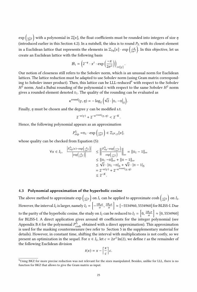
exp

(.

2σ 2

)with a polynomial in Z[x], the float coefficients must be rounded into integers of size η

(introduced earlier in this Section 4.2). In a nutshell, the idea is to round PR with its closest element

in a Euclidean lattice that represents the elements in Z2η[x] · exp(−x2σ 2

). In this objective, let us

create an Euclidean lattice with the following basis

B1 =(2−η · x i · exp

(−x

2σ 2

))i ∈[γ ].

Our notion of closeness still refers to the Sobolev norm, which is an unusual norm for Euclidean

lattices. The lattice reduction must be adapted to use Sobolev norm (using Gram matrix correspond-

ing to Sobolev inner product). Then, this lattice can be LLL-reduced9with respect to the Sobolev

H 2norm. And a Babai rounding of the polynomial Π with respect to the same Sobolev H 2

norm

gives a rounded element denoted ΠZ. The quality of the rounding can be evaluated as

κround(γ ,η) = − log2

(√2 ·

��ΠZ −Π��S ) .Finally, η must be chosen and the degree γ can be modified s.t.

2−κ(γ ) + 2−κ

round(γ ,η) < 2−K .

Hence, the following polynomial appears as an approximation

P I1exp=ΠZ · exp

(.

2σ 2

)∈ Z2η,γ [x].

whose quality can be checked from Equation (5):

∀x ∈ I1,���P I1exp(x )−exp( x

2σ 2

)������exp( x2σ 2

)��� ≤

������ P I1exp−exp( .2σ 2

)exp

(.

2σ 2

) ������∞= ∥ΠZ − 1∥∞

≤ ∥ΠZ −Π∥∞ + ∥Π − 1∥∞

≤√2 · |ΠZ −Π |S +

√2 · |Π − 1|

S

= 2−κ(γ ) + 2−κ

round(γ ,η)

≤ 2−K .

4.3 Polynomial approximation of the hyperbolic cosine

The above method to approximate exp

(.

2σ 2

)on I1 can be applied to approximate cosh

(.

2σ 2

)on I2.

However, the interval I2 is larger, namely I2 =[−

2B2σα ,

2B2σα

]≈ [−5534960, 5534960] for BLISS-I. Due

to the parity of the hyperbolic cosine, the study on I2 can be reduced to I2 =[0, 2B2σ

α

]≈ [0, 5534960]

for BLISS-I. A direct application gives around 48 coefficients for the integer polynomial (see

Appendix B.4 for the polynomial P I2cosh

obtained with a direct approximation). This approximation

is used for the masking countermeasure (we refer to Section 5 in the supplementary material for

details). However, in constant time, shifting the interval with multiplications is not costly, so we

present an optimization in the sequel. For x ∈ I2, let c = 2σ 2ln(2), we define t as the remainder of

the following Euclidean division

t(x) = x −⌈xc

⌉c .

9Using BKZ for more precise reduction was not relevant for the sizes manipulated. Besides, unlike for LLL, there is no

function for BKZ that allows to give the Gram matrix as input.

25

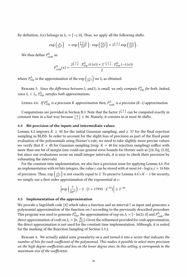
By definition, t(x) belongs in I3 := [−c, 0]. Thus, we apply all the following shifts.

exp

(x2σ 2

)= exp

(⌊ xc ⌋c2σ 2

)· exp

(t (x )2σ 2

)= 2⌊ xc ⌋ exp

(t (x )2σ 2

).

We thus define P I2cosh

as

P I2cosh(x) =

2⌊ xc ⌋ · P I3

exp(t (x)) + 2−⌊

xc ⌋ · P I3

exp(−t (x))

2

where P I3exp

is the approximation of the exp

(.

2σ 2

)on I3 as obtained.

Remark 3. Since the difference between I1 and I3 is small, we only compute P I3exp

for both. Indeed,

since I1 ⊂ I3, PI3exp

satisfies both approximations.

Lemma 4.6. If P I3exp

is a precision K approximation then, P I2cosh

is a precision (K-1) approximation.

Computations are provided in Section B.3. Note that the factor 2⌊ xc ⌋ can be computed exactly in

constant time in a fast way because

⌊ xc

⌋≤ 86. Namely, it consists in at most 86 shifts.

4.4 Bit precision of the inputs and intermediate valuesLemma 4.2 imposes K ≥ 45 for the initial Gaussian sampling, and ≥ 37 for the final rejection

sampling in BLISS. In order to account for the slight loss of precision as part of the fixed point

evaluation of the polynomials using Horner’s rule, we need to take slightly more precise values:

we verify that K = 48 for Gaussian sampling (resp. K = 40 for rejection sampling) suffice with

more than one bit of margin (one could use general error bounds for Horner such as [24, Eq. (5.3)],

but since our evaluations occur on small integer intervals, it is easy to check their precision by

exhausting the intervals).

For the constant time implementation, we also face a precision issue for applying Lemma 4.6. For

an implementation with 64 bits integers, the value c can be stored with at most 64− log(x2) = 16 bits

of precision. Thus, exp

(c

2σ 2

)is not exactly equal to 2. To preserve Lemma 4.6’s K − 1 bit security,

we simply use a first order approximation of the exponential at c:���exp ( c

2σ 2

)− 2 ·

(1 + 17933 · 2−43

) ��� ≤ 2−46.

4.5 Implementation of the approximationWe provide a SageMath code [4] which takes a function and an interval I as input and generates a

polynomial approximation of the function on I according to the previously described procedure.

This program was used to generate P I3exp

, the approximation of exp on I3 = [− ln(2), 0] and PI2cosh

, the

direct approximation of cosh on I2 = [0,B2

σα ]. Given the refinement provided for cosh approximation,

the direct approximation is not used for the constant time implementation. Although, it is suited

for the masking of the Rejection Sampling of Section 5.3.2.

Remark 4. We actually added some granularity on η and turned it into a vector that indicates the

number of bits for each coefficient of the polynomial. This makes it possible to select more precision

on the high degree coefficients and less on the lower degree ones. In this setting, η corresponds to the

maximum size of the coefficients.

26

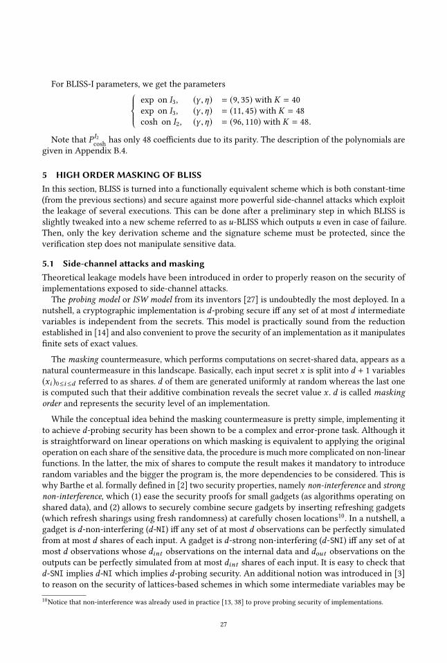
For BLISS-I parameters, we get the parametersexp on I3, (γ ,η) = (9, 35) with K = 40

exp on I3, (γ ,η) = (11, 45) with K = 48

cosh on I2, (γ ,η) = (96, 110) with K = 48.

Note that P I2cosh

has only 48 coefficients due to its parity. The description of the polynomials are

given in Appendix B.4.

5 HIGH ORDER MASKING OF BLISSIn this section, BLISS is turned into a functionally equivalent scheme which is both constant-time

(from the previous sections) and secure against more powerful side-channel attacks which exploit

the leakage of several executions. This can be done after a preliminary step in which BLISS is

slightly tweaked into a new scheme referred to as u-BLISS which outputs u even in case of failure.

Then, only the key derivation scheme and the signature scheme must be protected, since the

verification step does not manipulate sensitive data.

5.1 Side-channel attacks and maskingTheoretical leakage models have been introduced in order to properly reason on the security of

implementations exposed to side-channel attacks.

The probing model or ISW model from its inventors [27] is undoubtedly the most deployed. In a

nutshell, a cryptographic implementation is d-probing secure iff any set of at most d intermediate

variables is independent from the secrets. This model is practically sound from the reduction

established in [14] and also convenient to prove the security of an implementation as it manipulates

finite sets of exact values.

The masking countermeasure, which performs computations on secret-shared data, appears as a

natural countermeasure in this landscape. Basically, each input secret x is split into d + 1 variables(xi )0≤i≤d referred to as shares. d of them are generated uniformly at random whereas the last one

is computed such that their additive combination reveals the secret value x . d is called masking

order and represents the security level of an implementation.

While the conceptual idea behind the masking countermeasure is pretty simple, implementing it

to achieve d-probing security has been shown to be a complex and error-prone task. Although it

is straightforward on linear operations on which masking is equivalent to applying the original

operation on each share of the sensitive data, the procedure is much more complicated on non-linear

functions. In the latter, the mix of shares to compute the result makes it mandatory to introduce

random variables and the bigger the program is, the more dependencies to be considered. This is

why Barthe et al. formally defined in [2] two security properties, namely non-interference and strong

non-interference, which (1) ease the security proofs for small gadgets (as algorithms operating on

shared data), and (2) allows to securely combine secure gadgets by inserting refreshing gadgets

(which refresh sharings using fresh randomness) at carefully chosen locations10. In a nutshell, a

gadget is d-non-interfering (d-NI) iff any set of at most d observations can be perfectly simulated

from at most d shares of each input. A gadget is d-strong non-interfering (d-SNI) iff any set of at

most d observations whose dint observations on the internal data and dout observations on the

outputs can be perfectly simulated from at most dint shares of each input. It is easy to check that

d-SNI implies d-NI which implies d-probing security. An additional notion was introduced in [3]

to reason on the security of lattices-based schemes in which some intermediate variables may be

10Notice that non-interference was already used in practice [13, 38] to prove probing security of implementations.

27

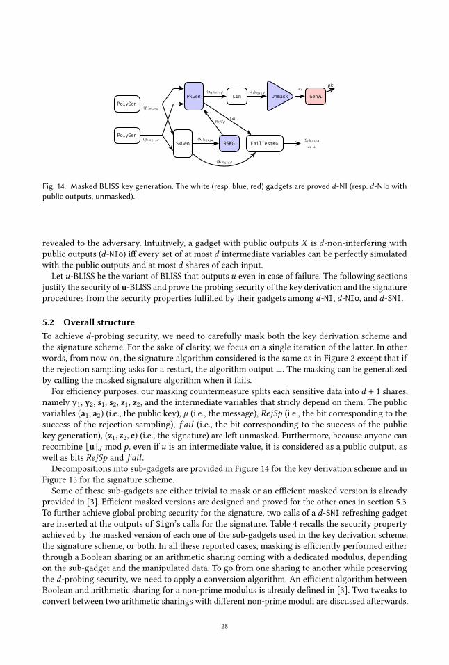
SkGen

PkGen

PolyGen

PolyGen

RSKG FailTestKG

Lin Unmask GenA

(fi )0≤i≤d

(дi )0≤i≤d (Si )0≤i≤d

(aq )0≤i≤d (a1)0≤i≤da1

pk

f ailRe jSp

(Si )0≤i≤dor ⊥

(Si )0≤i≤d

Fig. 14. Masked BLISS key generation. The white (resp. blue, red) gadgets are proved d-NI (resp. d-NIo withpublic outputs, unmasked).

revealed to the adversary. Intuitively, a gadget with public outputs X is d-non-interfering with

public outputs (d-NIo) iff every set of at most d intermediate variables can be perfectly simulated

with the public outputs and at most d shares of each input.

Let u-BLISS be the variant of BLISS that outputs u even in case of failure. The following sections

justify the security of u-BLISS and prove the probing security of the key derivation and the signatureprocedures from the security properties fulfilled by their gadgets among d-NI, d-NIo, and d-SNI.

5.2 Overall structureTo achieve d-probing security, we need to carefully mask both the key derivation scheme and

the signature scheme. For the sake of clarity, we focus on a single iteration of the latter. In other

words, from now on, the signature algorithm considered is the same as in Figure 2 except that if

the rejection sampling asks for a restart, the algorithm output ⊥. The masking can be generalized

by calling the masked signature algorithm when it fails.

For efficiency purposes, our masking countermeasure splits each sensitive data into d + 1 shares,namely y1, y2, s1, s2, z1, z2, and the intermediate variables that stricly depend on them. The public

variables (a1, a2) (i.e., the public key), µ (i.e., the message), RejSp (i.e., the bit corresponding to the

success of the rejection sampling), f ail (i.e., the bit corresponding to the success of the public

key generation), (z1, z2, c) (i.e., the signature) are left unmasked. Furthermore, because anyone can

recombine ⌊u⌉d mod p, even if u is an intermediate value, it is considered as a public output, as

well as bits RejSp and f ail .Decompositions into sub-gadgets are provided in Figure 14 for the key derivation scheme and in

Figure 15 for the signature scheme.

Some of these sub-gadgets are either trivial to mask or an efficient masked version is already

provided in [3]. Efficient masked versions are designed and proved for the other ones in section 5.3.

To further achieve global probing security for the signature, two calls of a d-SNI refreshing gadget

are inserted at the outputs of Sign’s calls for the signature. Table 4 recalls the security property

achieved by the masked version of each one of the sub-gadgets used in the key derivation scheme,

the signature scheme, or both. In all these reported cases, masking is efficiently performed either

through a Boolean sharing or an arithmetic sharing coming with a dedicated modulus, depending

on the sub-gadget and the manipulated data. To go from one sharing to another while preserving

the d-probing security, we need to apply a conversion algorithm. An efficient algorithm between

Boolean and arithmetic sharing for a non-prime modulus is already defined in [3]. Two tweaks to

convert between two arithmetic sharings with different non-prime moduli are discussed afterwards.

28

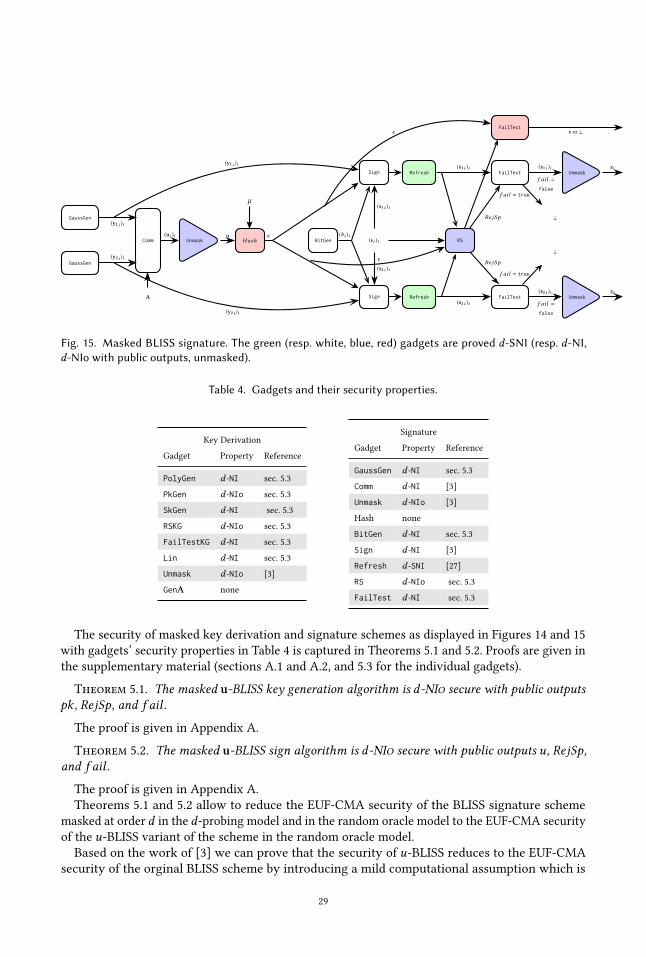
Unmask

GaussGen

GaussGen

RS

Unmask

Unmask

FailTest

FailTest

FailTest

HashComm BitGen

Sign

Sign

Refresh

Refresh

µ

Re jSp

Re jSp

⊥

⊥

f ail = true

f ail = true

f ail =

false

f ail =

false

(y1i )i

(y2i )i

(ui )i u

(z1i )i

(z2i )i

c

z1

z2

(z1i )i

(z2i )i

(y1i )i

(y2i )i

A

(bi )i(si )i

(s1i )i

(s2i )i

c

c

c or ⊥

Fig. 15. Masked BLISS signature. The green (resp. white, blue, red) gadgets are proved d-SNI (resp. d-NI,d-NIo with public outputs, unmasked).

Table 4. Gadgets and their security properties.

Key Derivation

Gadget Property Reference

PolyGen d -NI sec. 5.3

PkGen d -NIo sec. 5.3

SkGen d -NI sec. 5.3

RSKG d -NIo sec. 5.3

FailTestKG d -NI sec. 5.3

Lin d -NI sec. 5.3

Unmask d -NIo [3]

GenA none

Signature

Gadget Property Reference

GaussGen d -NI sec. 5.3

Comm d -NI [3]

Unmask d -NIo [3]

Hash none

BitGen d -NI sec. 5.3

Sign d -NI [3]

Refresh d -SNI [27]

RS d -NIo sec. 5.3

FailTest d -NI sec. 5.3

The security of masked key derivation and signature schemes as displayed in Figures 14 and 15

with gadgets’ security properties in Table 4 is captured in Theorems 5.1 and 5.2. Proofs are given in

the supplementary material (sections A.1 and A.2, and 5.3 for the individual gadgets).

Theorem 5.1. The masked u-BLISS key generation algorithm is d-NIo secure with public outputs

pk , RejSp, and f ail .

The proof is given in Appendix A.

Theorem 5.2. The masked u-BLISS sign algorithm is d-NIo secure with public outputs u, RejSp,and f ail .

The proof is given in Appendix A.

Theorems 5.1 and 5.2 allow to reduce the EUF-CMA security of the BLISS signature scheme

masked at order d in the d-probing model and in the random oracle model to the EUF-CMA security

of the u-BLISS variant of the scheme in the random oracle model.

Based on the work of [3] we can prove that the security of u-BLISS reduces to the EUF-CMA

security of the orginal BLISS scheme by introducing a mild computational assumption which is

29

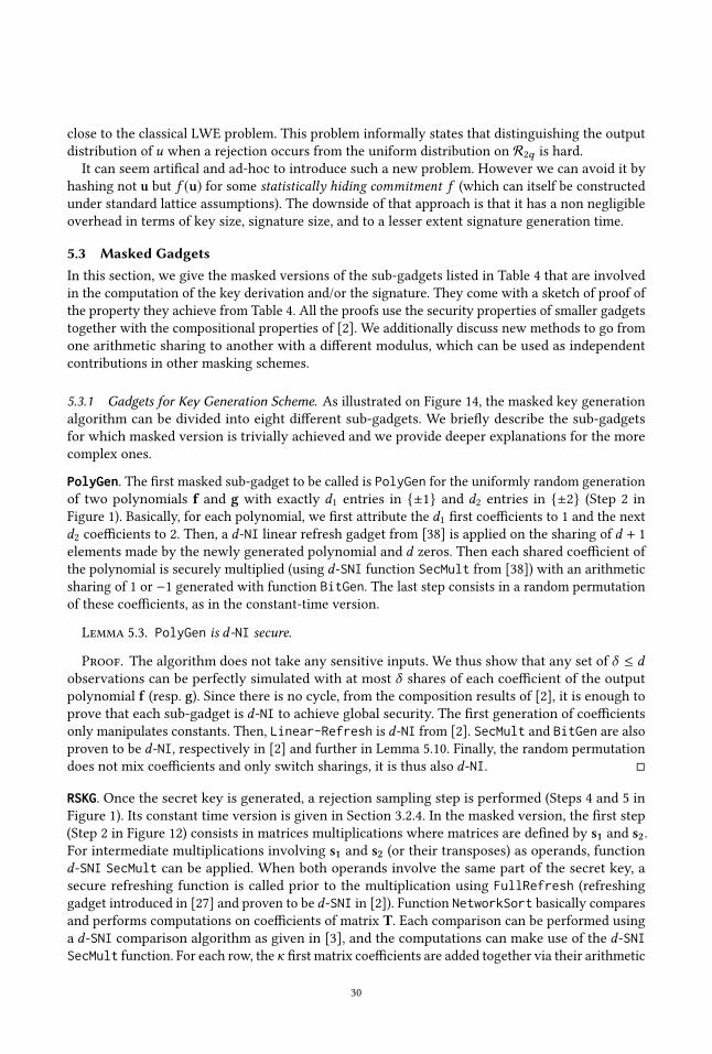
close to the classical LWE problem. This problem informally states that distinguishing the output

distribution of u when a rejection occurs from the uniform distribution on R2q is hard.

It can seem artifical and ad-hoc to introduce such a new problem. However we can avoid it by

hashing not u but f (u) for some statistically hiding commitment f (which can itself be constructed

under standard lattice assumptions). The downside of that approach is that it has a non negligible

overhead in terms of key size, signature size, and to a lesser extent signature generation time.

5.3 Masked GadgetsIn this section, we give the masked versions of the sub-gadgets listed in Table 4 that are involved

in the computation of the key derivation and/or the signature. They come with a sketch of proof of

the property they achieve from Table 4. All the proofs use the security properties of smaller gadgets

together with the compositional properties of [2]. We additionally discuss new methods to go from

one arithmetic sharing to another with a different modulus, which can be used as independent

contributions in other masking schemes.

5.3.1 Gadgets for Key Generation Scheme. As illustrated on Figure 14, the masked key generation

algorithm can be divided into eight different sub-gadgets. We briefly describe the sub-gadgets

for which masked version is trivially achieved and we provide deeper explanations for the more

complex ones.

PolyGen. The first masked sub-gadget to be called is PolyGen for the uniformly random generation

of two polynomials f and g with exactly d1 entries in {±1} and d2 entries in {±2} (Step 2 in

Figure 1). Basically, for each polynomial, we first attribute the d1 first coefficients to 1 and the next

d2 coefficients to 2. Then, a d-NI linear refresh gadget from [38] is applied on the sharing of d + 1elements made by the newly generated polynomial and d zeros. Then each shared coefficient of

the polynomial is securely multiplied (using d-SNI function SecMult from [38]) with an arithmetic

sharing of 1 or −1 generated with function BitGen. The last step consists in a random permutation

of these coefficients, as in the constant-time version.

Lemma 5.3. PolyGen is d-NI secure.

Proof. The algorithm does not take any sensitive inputs. We thus show that any set of δ ≤ dobservations can be perfectly simulated with at most δ shares of each coefficient of the output

polynomial f (resp. g). Since there is no cycle, from the composition results of [2], it is enough to

prove that each sub-gadget is d-NI to achieve global security. The first generation of coefficients

only manipulates constants. Then, Linear-Refresh is d-NI from [2]. SecMult and BitGen are alsoproven to be d-NI, respectively in [2] and further in Lemma 5.10. Finally, the random permutation

does not mix coefficients and only switch sharings, it is thus also d-NI. □

RSKG. Once the secret key is generated, a rejection sampling step is performed (Steps 4 and 5 in

Figure 1). Its constant time version is given in Section 3.2.4. In the masked version, the first step

(Step 2 in Figure 12) consists in matrices multiplications where matrices are defined by s1 and s2.For intermediate multiplications involving s1 and s2 (or their transposes) as operands, functiond-SNI SecMult can be applied. When both operands involve the same part of the secret key, a

secure refreshing function is called prior to the multiplication using FullRefresh (refreshing

gadget introduced in [27] and proven to be d-SNI in [2]). Function NetworkSort basically compares

and performs computations on coefficients of matrix T. Each comparison can be performed using

a d-SNI comparison algorithm as given in [3], and the computations can make use of the d-SNISecMult function. For each row, theκ first matrix coefficients are added together via their arithmetic

30

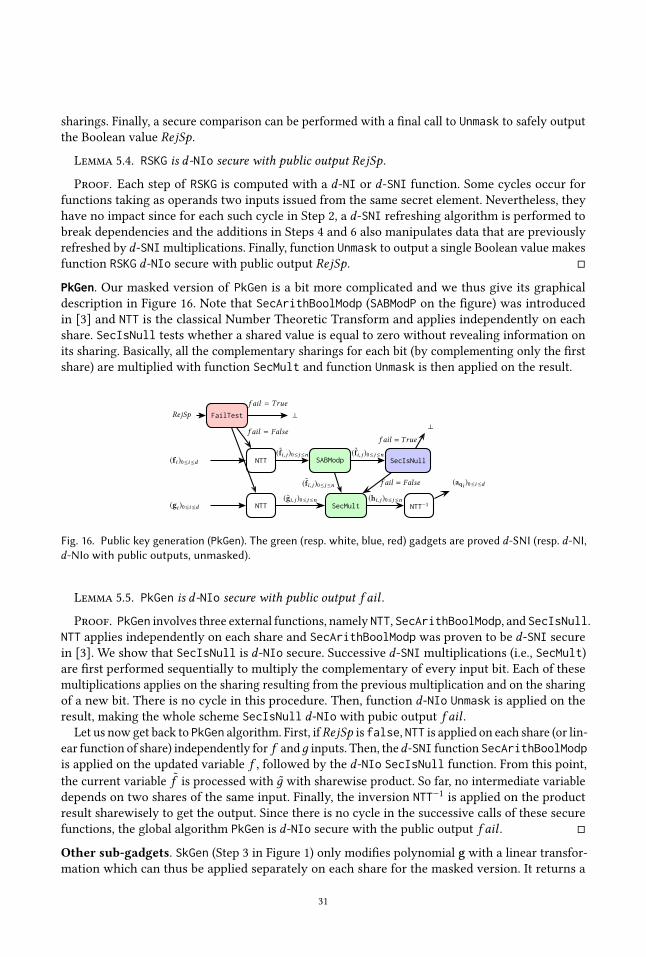
sharings. Finally, a secure comparison can be performed with a final call to Unmask to safely output

the Boolean value RejSp.

Lemma 5.4. RSKG is d-NIo secure with public output RejSp.

Proof. Each step of RSKG is computed with a d-NI or d-SNI function. Some cycles occur for

functions taking as operands two inputs issued from the same secret element. Nevertheless, they

have no impact since for each such cycle in Step 2, a d-SNI refreshing algorithm is performed to

break dependencies and the additions in Steps 4 and 6 also manipulates data that are previously

refreshed by d-SNImultiplications. Finally, function Unmask to output a single Boolean value makes

function RSKG d-NIo secure with public output RejSp. □

PkGen. Our masked version of PkGen is a bit more complicated and we thus give its graphical

description in Figure 16. Note that SecArithBoolModp (SABModP on the figure) was introduced

in [3] and NTT is the classical Number Theoretic Transform and applies independently on each

share. SecIsNull tests whether a shared value is equal to zero without revealing information on

its sharing. Basically, all the complementary sharings for each bit (by complementing only the first

share) are multiplied with function SecMult and function Unmask is then applied on the result.

FailTest

NTT

NTT

SABModp SecIsNull

SecMult NTT−1

RejSp

(fi )0≤i≤d

(gi )0≤i≤d

f ail = False

f ail = True

⊥

(f̃i, j )0≤j≤n

(g̃i, j )0≤j≤n

(f̃i, j )0≤j≤n

(f̃i, j )0≤j≤n

(hi, j )0≤j≤n

f ail = False

⊥

f ail = True

(aqi )0≤i≤d

Fig. 16. Public key generation (PkGen). The green (resp. white, blue, red) gadgets are proved d-SNI (resp. d-NI,d-NIo with public outputs, unmasked).

Lemma 5.5. PkGen is d-NIo secure with public output f ail .

Proof. PkGen involves three external functions, namely NTT, SecArithBoolModp, and SecIsNull.NTT applies independently on each share and SecArithBoolModp was proven to be d-SNI securein [3]. We show that SecIsNull is d-NIo secure. Successive d-SNI multiplications (i.e., SecMult)are first performed sequentially to multiply the complementary of every input bit. Each of these

multiplications applies on the sharing resulting from the previous multiplication and on the sharing

of a new bit. There is no cycle in this procedure. Then, function d-NIo Unmask is applied on the

result, making the whole scheme SecIsNull d-NIo with pubic output f ail .Let us now get back to PkGen algorithm. First, ifRejSp is false, NTT is applied on each share (or lin-

ear function of share) independently for f andд inputs. Then, thed-SNI function SecArithBoolModpis applied on the updated variable f , followed by the d-NIo SecIsNull function. From this point,

the current variable˜f is processed with д̃ with sharewise product. So far, no intermediate variable

depends on two shares of the same input. Finally, the inversion NTT−1 is applied on the product

result sharewisely to get the output. Since there is no cycle in the successive calls of these secure

functions, the global algorithm PkGen is d-NIo secure with the public output f ail . □

Other sub-gadgets. SkGen (Step 3 in Figure 1) only modifies polynomial g with a linear transfor-

mation which can thus be applied separately on each share for the masked version. It returns a

31

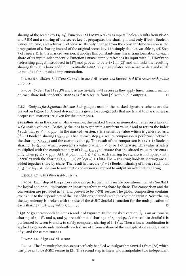
sharing of the secret key (s1, s2). Function FailTestKG takes as inputs Boolean results from PkGenand RSKG and a sharing of the secret key. It propagates the sharing if and only if both Boolean

values are true, and returns ⊥ otherwise. Its only change from the constant-time version is the

propagation of a sharing instead of the original secret key. Lin simply doubles variable aq (cf. Step

7 of Figure 1). In the masked version, it applies this constant-time linear transformation on each

share of its input independently. Function Unmask simply refreshes its input with FullRefresh(refreshing gadget introduced in [27] and proven to be d-SNI in [2]) and unmasks the resulting

sharing through a basic addition. Eventually, GenA only manipulates non-sensitive data and is left

unmodified for a masked implementation.

Lemma 5.6. SkGen, FailTestKG and Lin are d-NI secure, and Unmask is d-NIo secure with public

output a1.

Proof. SkGen, FailTestKG and Lin are trivially d-NI secure as they apply linear transformation

on each share independently. Unmask is d-NIo secure from [3] with public output a1. □

5.3.2 Gadgets for Signature Scheme. Sub-gadgets used in the masked signature scheme are dis-

played on Figure 15. A brief description is given for sub-gadgets that are trivial to mask whereas

deeper explanations are given for the other ones.

GaussGen. As in the constant-time version, the masked Gaussian generation relies on a table of

w Gaussian values pj . Basically the idea is to generate a uniform value r and to return the index

j such that pj ≤ r < pj+1. In the masked version, r is a sensitive value which is generated as a

(d + 1) Boolean sharing (ri )0≤i≤d . Then at each step j, a secure comparison is performed between

the sharing (ri )0≤i≤d and the current value pj . The result of the comparison is a (d + 1) Booleansharing (bj,i )0≤i≤d which represents a value 0 when r < pj or 1 otherwise. This value is safelymultiplied with the complementary of (bj−1,i )0≤i≤d to ensure that the shared value represents 1

only when pj ≤ r < pj+1. At that point, for 1 ≤ j ≤ w , each sharing (bj,i )0≤i≤d is multiplied (with

SecMult) with the sharing (j, 0, . . . , 0) on log(w) + 1 bits. Thew resulting Boolean sharings are all

added together share by share. The result is a secure (d + 1) Boolean sharing of index j such that

pj ≤ r < pj+1. A Boolean to arithmetic conversion is applied to output an arithmetic sharing.

Lemma 5.7. GaussGen is d-NI secure.

Proof. Each step of the process above is performed with secure operations, namely SecMultfor logical and or multiplications or linear transformations share by share. The comparison and the

conversion are provided in [3] and proven to be d-SNI secure. The global composition contains

cycles due to the dependency of the last additions operands with the common input r . Nevertheless,the dependency is broken with the use of the d-SNI SecMult function for the multiplication of

each sharing (bj,i )0≤i≤d with (j, 0, . . . , 0). □

Sign. Sign corresponds to Steps 6 and 7 of Figure 2. In the masked version,˜bi is an arithmetic

sharing of (−1)b , and si and yi are arithmetic sharings of si and yi . A first call to SecMult is

performed between˜bi and si to safely compute a sharing of (−1)bsi . Then a linear combination is

applied to generate independently each share of z from a share of the multiplication result, a share

of yi, and the commitment c.

Lemma 5.8. Sign is d-NI secure.

Proof. The first multiplication step is perfectly handled with algorithm SecMult from [38] which

was proven to be d-SNI secure in [2]. The second step is linear and manipulates two independent

32

inputs (an input of Sign and the output of a d-SNI gadget) share by share. It is thus d-NI. Theabsence of cycles makes the masked version of Sign d-NI secure from the compositional properties

established in [2]. □

RS. The steps which compose the constant-time version of RS are given in Section 4. They can

easily be transformed to ensure d-probing security. Step 1 computes two elements x1 and x2 fromsensitive values s and z. Multiplications must be processed with function SecMult in the masked

version. As for Step 2, two sets of d+1 Boolean shares are generated at random in {0, 1} to representthe secret bits u1 and u2. Steps 3 and 4 require the computation of exp(x1) and cosh(x2) with x1and x2 sensitive values shared in Step 1. Thanks to the polynomial approximation of these two

functions, as described in Section 4, the evaluation of exp and cosh for these two sharings is only a

combination of linear squarings and SecMult operations. As for their comparison with functions of

u1 and u2, the computed arithmetic sharings are first converted into Boolean sharings as suggested

in [3] (sharing of u1 can be first converted into an arithmetic masking to be subtracted to exp(x1)and allows a comparison with public values). Then, a secure comparison is performed between

Boolean sharings and outputs two masked bits of a and b. Finally, the last multiplication in Step 5

is computed with SecMult, before a call to Unmask outputs RejSp.

Lemma 5.9. RS is d-NIo secure with the public output RejSp.

Proof. All the steps in RS are either d-NI secure (random generations of Boolean sharings),

d-NIo secure (Unmask) or d-SNI secure (masking conversions, comparisons, polynomial evaluation,

and multiplication). Thus, it is enough that each cycle is properly handled. Basically, the algorithm

produces one cycle since the logical and of both Boolean values a and b takes as input variables

that both depend on the secret key. Nevertheless, both multiplication inputs are refreshed with

d-SNI gadgets which is enough to break the dependency. □

Other Gadgets. The commitment function Comm takes as inputs two arithmetic sharings and the

public key. The linear transformation applied in the unmasked version (Step 3, Figure 2) is here

applied on each share of the secret inputs. As proven in [3], function Unmask is d-NIo secure with

public output a signature part or u. Hash applies on a public output, so it is left unchanged in the

masked version. BitGen first generates d + 1 bits uniformly at random to build a Boolean sharing

of a value in {0, 1}. The resulting sharing is then converted into an arithmetic sharing using the

secure conversion method provided in [3]. In the masked version of the signature, FailTest simply

returns ⊥ if RejSp is true and the input sharing (zi )0≤i≤d or c otherwise.

Lemma 5.10. Comm, BitGen, and FailTest are d-NI secure and Unmask is d-NIo secure with the

public output a signature part or u.

Proof. Functions Comm and FailTest manipulates shares separately and thus are trivially d-NIsecure. The first step of BitGen separately generates uniform random bits. They are then processed

in a d-SNI secure conversion function as proven in [3]. BitGen is thus (at least) d-NI secure. Unmaskis d-NIo secure from [3] with public output u or the signature. □

5.3.3 Masking Conversion. The state of the art provides efficient techniques to convert Boolean

masking into arithmetic masking with power-of-two modulus and the reverse for higher-order

implementations [12]. A recent paper additionally extends these tools to convert from Booleanmask-

ing to arithmetic masking with any modulus [3]. To efficiently mask the polynomial approximation

in our constant-time implementation of BLISS, we need an unusual conversion between arithmetic

masking with a modulus q and arithmetic masking with a modulus q′ ≫ q. Our approximations

being of high degrees, we need to update our modulus accordingly. One easy way to do it is to

33

convert the first arithmetic masking with modulus q into a Boolean masking and then to convert it

back to the second arithmetic masking with modulus q′. This requires two full conversions. Anotherpossible method is to adapt one of the conversion algorithms given in [12] and extended in [3]

for any modulus to an arithmetic to arithmetic masking. The only step to modify is the operation

SecAdd which takes two Boolean sharings of x and y in inputs and outputs a Boolean sharing of zsuch that z = x + y with the arithmetic modulus. In our case, the Boolean sharings are replaced by

arithmetic sharings with a modulus q′ and the arithmetic addition to perform is to be done with

a modulus q ≪ q′. Namely, we have two arithmetic sharings (xi )0≤i≤d and (yi )0≤i≤d modulo q′

of values x and y and we want to obtain an arithmetic (zi )0≤i≤d modulo q′ of a value z such that

z = x + y mod q. Basically, we can perform an arithmetic addition modulo q of the lowest part

(i.e., the less significant bits) of x and y’s sharings to avoid the carry management. Then, only the

highest part (i.e., the most significant bits) of the sharings are to be converted into Boolean shares.

The addition is then performed as in the paper [3] and a final Boolean to arithmetic conversion

ends the operation. Note that in this case, we also need to have an arithmetic to Boolean and a

Boolean to arithmetic conversions. However, these two conversions are dependent on the number

of bits to convert. And by saving the less significant bits of the sharings, both conversions are

cheaper. Concretely, as x and y are values between 0 and q − 1, we can save log2(q) − log

2(2(d + 1))

bits in the lowest part, leaving log2(q′) − log

2(q) + log

2(2(d + 1)) to convert.

6 ACKNOWLEDGEMENTSWe thank the anonymous reviewers for their very relevant comments and their analysis of our

code. We acknowledge the support of the French Programme d’Investissement d’Avenir under

national project RISQ P14158. This work is also partially supported by the European Union’s H2020

Programme under grant agreement number ERC-669891 and the PROMETHEUS project (grant

780701), and by the French FUI-AAP25 VERISICC project. This research has been partially funded

by ANRT under the programs CIFRE N 2016/1583. This work was partially supported by Office of

Naval Research under projects N00014-12-1-0914, N00014-15-1-2750 and N00014-19-1-2292.

REFERENCES[1] Erdem Alkim, Paulo S. L. M. Barreto, Nina Bindel, Patrick Longa, and Jefferson E. Ricardini. 2019. The lattice-based

digital signature scheme qTESLA. Cryptology ePrint Archive, Report 2019/085. https://eprint.iacr.org/2019/085.

[2] Gilles Barthe, Sonia Belaïd, François Dupressoir, Pierre-Alain Fouque, Benjamin Grégoire, Pierre-Yves Strub, and

Rébecca Zucchini. 2016. Strong Non-Interference and Type-Directed Higher-Order Masking. In ACM CCS 2016, Edgar R.

Weippl, Stefan Katzenbeisser, Christopher Kruegel, Andrew C. Myers, and Shai Halevi (Eds.). ACM Press, 116–129.

https://doi.org/10.1145/2976749.2978427

[3] Gilles Barthe, Sonia Belaïd, Thomas Espitau, Pierre-Alain Fouque, Benjamin Grégoire, Mélissa Rossi, and Mehdi

Tibouchi. 2018. Masking the GLP Lattice-Based Signature Scheme at Any Order. In EUROCRYPT 2018, Part II (LNCS),

Jesper Buus Nielsen and Vincent Rijmen (Eds.), Vol. 10821. Springer, Heidelberg, 354–384. https://doi.org/10.1007/978-

3-319-78375-8_12

[4] Gilles Barthes, Sonia Belaïd, Thomas Espitau, Mélissa Rossi, and Mehdi Tibouchi. 2019. GALACTICS implementations.

https://github.com/espitau/GALACTICS

[5] Daniel J. Bernstein and VAMPIRE Lab others. 2016. System for Unified Performance Evaluation Related to Cryptographic

Operations and Primitives. https://bench.cr.yp.to/supercop.html.

[6] Jonathan Bootle, Claire Delaplace, Thomas Espitau, Pierre-Alain Fouque, and Mehdi Tibouchi. 2018. LWE Without

Modular Reduction and Improved Side-Channel Attacks Against BLISS. In ASIACRYPT 2018, Part I (LNCS), Thomas

Peyrin and Steven Galbraith (Eds.), Vol. 11272. Springer, Heidelberg, 494–524. https://doi.org/10.1007/978-3-030-

03326-2_17

[7] Joppe W. Bos. 2014. Constant time modular inversion. Journal of Cryptographic Engineering 4, 4 (Nov. 2014), 275–281.

https://doi.org/10.1007/s13389-014-0084-8

[8] Nicolas Brisebarre and Sylvain Chevillard. 2018. Efficient polynomial L∞-approximations. In 18th IEEE Symposium on

Computer Arithmetic (ARITH 18). IEEE, 169–176.

34

[9] Leon Groot Bruinderink, Andreas Hülsing, Tanja Lange, and Yuval Yarom. 2016. Flush, Gauss, and Reload - A Cache

Attack on the BLISS Lattice-Based Signature Scheme. In CHES 2016 (LNCS), Benedikt Gierlichs and Axel Y. Poschmann

(Eds.), Vol. 9813. Springer, Heidelberg, 323–345. https://doi.org/10.1007/978-3-662-53140-2_16

[10] E. J. Candés, X. Li, and M. Soltanolkotabi. 2015. Phase Retrieval via Wirtinger Flow: Theory and Algorithms. IEEE

Transactions on Information Theory 61, 4 (2015), 1985–2007.

[11] S. Chevillard, M. Joldeş, and C. Lauter. 2010. Sollya: An Environment for the Development of Numerical Codes. In

Mathematical Software - ICMS 2010 (Lecture Notes in Computer Science), K. Fukuda, J. van der Hoeven, M. Joswig, and

N. Takayama (Eds.), Vol. 6327. Springer, Heidelberg, Germany, 28–31.

[12] Jean-Sébastien Coron, Johann Großschädl, and Praveen Kumar Vadnala. 2014. Secure Conversion between Boolean

and Arithmetic Masking of Any Order. In CHES 2014 (LNCS), Lejla Batina and Matthew Robshaw (Eds.), Vol. 8731.

Springer, Heidelberg, 188–205. https://doi.org/10.1007/978-3-662-44709-3_11

[13] Jean-Sébastien Coron, Emmanuel Prouff, Matthieu Rivain, and Thomas Roche. 2014. Higher-Order Side Channel

Security and Mask Refreshing. In FSE 2013 (LNCS), Shiho Moriai (Ed.), Vol. 8424. Springer, Heidelberg, 410–424.

https://doi.org/10.1007/978-3-662-43933-3_21

[14] Alexandre Duc, Stefan Dziembowski, and Sebastian Faust. 2014. Unifying Leakage Models: From Probing Attacks

to Noisy Leakage. In EUROCRYPT 2014 (LNCS), Phong Q. Nguyen and Elisabeth Oswald (Eds.), Vol. 8441. Springer,

Heidelberg, 423–440. https://doi.org/10.1007/978-3-642-55220-5_24

[15] Léo Ducas. 2014. Accelerating Bliss: the geometry of ternary polynomials. Cryptology ePrint Archive, Report 2014/874.

http://eprint.iacr.org/2014/874.

[16] Léo Ducas, Alain Durmus, Tancrède Lepoint, and Vadim Lyubashevsky. 2013. Lattice Signatures and Bimodal

Gaussians. In CRYPTO 2013, Part I (LNCS), Ran Canetti and Juan A. Garay (Eds.), Vol. 8042. Springer, Heidelberg, 40–56.

https://doi.org/10.1007/978-3-642-40041-4_3

[17] Léo Ducas, Steven Galbraith, Thomas Prest, and Yang Yu. 2019. Integral matrix Gram root and lattice Gaussian

sampling without floats. Cryptology ePrint Archive, Report 2019/320. https://eprint.iacr.org/2019/320.

[18] Léo Ducas, Eike Kiltz, Tancrède Lepoint, Vadim Lyubashevsky, Peter Schwabe, Gregor Seiler, and Damien Stehlé.

2018. CRYSTALS-Dilithium: A Lattice-Based Digital Signature Scheme. IACR TCHES 2018, 1 (2018), 238–268. https:

//doi.org/10.13154/tches.v2018.i1.238-268 https://tches.iacr.org/index.php/TCHES/article/view/839.

[19] Léo Ducas and Tancrède Lepoint. 2013. BLISS: Bimodal Lattice Signature Schemes. http://bliss.di.ens.fr/bliss-06-13-

2013.zip (original implementation).

[20] Léo Ducas and Phong Q. Nguyen. 2012. Faster Gaussian Lattice Sampling Using Lazy Floating-Point Arithmetic. In

ASIACRYPT 2012 (LNCS), Xiaoyun Wang and Kazue Sako (Eds.), Vol. 7658. Springer, Heidelberg, 415–432. https:

//doi.org/10.1007/978-3-642-34961-4_26

[21] Thomas Espitau, Pierre-Alain Fouque, Benoît Gérard, and Mehdi Tibouchi. 2018. Loop-Abort Faults on Lattice-Based

Signature Schemes and Key Exchange Protocols. IEEE Trans. Computers 67, 11 (2018), 1535–1549.

[22] Thomas Espitau, Pierre-Alain Fouque, Benoît Gérard, andMehdi Tibouchi. 2017. Side-Channel Attacks on BLISS Lattice-

Based Signatures: Exploiting Branch Tracing against strongSwan and Electromagnetic Emanations in Microcontrollers.

In ACM CCS 2017, Bhavani M. Thuraisingham, David Evans, Tal Malkin, and Dongyan Xu (Eds.). ACM Press, 1857–1874.

https://doi.org/10.1145/3133956.3134028

[23] TimGüneysu, Vadim Lyubashevsky, and Thomas Pöppelmann. 2012. Practical Lattice-Based Cryptography: A Signature

Scheme for Embedded Systems. In CHES 2012 (LNCS), Emmanuel Prouff and Patrick Schaumont (Eds.), Vol. 7428.

Springer, Heidelberg, 530–547. https://doi.org/10.1007/978-3-642-33027-8_31

[24] Nicholas J. Higham. 2002. Accuracy and Stability of Numerical Algorithms (second ed.). SIAM.

[25] Nick Howgrave-Graham. 2007. A Hybrid Lattice-Reduction and Meet-in-the-Middle Attack Against NTRU. In

CRYPTO 2007 (LNCS), Alfred Menezes (Ed.), Vol. 4622. Springer, Heidelberg, 150–169. https://doi.org/10.1007/978-3-

540-74143-5_9

[26] Andreas Hülsing, Tanja Lange, and Kit Smeets. 2018. Rounded Gaussians - Fast and Secure Constant-Time Sampling

for Lattice-Based Crypto. In PKC 2018, Part II (LNCS), Michel Abdalla and Ricardo Dahab (Eds.), Vol. 10770. Springer,

Heidelberg, 728–757. https://doi.org/10.1007/978-3-319-76581-5_25

[27] Yuval Ishai, Amit Sahai, and David Wagner. 2003. Private Circuits: Securing Hardware against Probing Attacks. In

CRYPTO 2003 (LNCS), Dan Boneh (Ed.), Vol. 2729. Springer, Heidelberg, 463–481. https://doi.org/10.1007/978-3-540-

45146-4_27

[28] Angshuman Karmakar, Sujoy Sinha Roy, Oscar Reparaz, Frederik Vercauteren, and Ingrid Verbauwhede. 2018. Constant-

Time Discrete Gaussian Sampling. IEEE Trans. Computers 67, 11 (2018), 1561–1571.

[29] Wangyu Luo,Wael Alghamdi, and YueM. Lu. 2019. Optimal Spectral Initialization for Signal RecoveryWithApplications

to Phase Retrieval. IEEE Trans. Signal Processing 67, 9 (2019), 2347–2356.

[30] Vadim Lyubashevsky. 2009. Fiat-Shamir with Aborts: Applications to Lattice and Factoring-Based Signatures. In

ASIACRYPT 2009 (LNCS), Mitsuru Matsui (Ed.), Vol. 5912. Springer, Heidelberg, 598–616. https://doi.org/10.1007/978-

35

3-642-10366-7_35

[31] Vadim Lyubashevsky. 2012. Lattice Signatures without Trapdoors. In EUROCRYPT 2012 (LNCS), David Pointcheval and

Thomas Johansson (Eds.), Vol. 7237. Springer, Heidelberg, 738–755. https://doi.org/10.1007/978-3-642-29011-4_43

[32] Daniele Micciancio and Michael Walter. 2017. Gaussian Sampling over the Integers: Efficient, Generic, Constant-Time.

In CRYPTO 2017, Part II (LNCS), Jonathan Katz and Hovav Shacham (Eds.), Vol. 10402. Springer, Heidelberg, 455–485.

https://doi.org/10.1007/978-3-319-63715-0_16

[33] Peter Pessl, Leon Groot Bruinderink, and Yuval Yarom. 2017. To BLISS-B or not to be: Attacking strongSwan’s

Implementation of Post-Quantum Signatures. In ACM CCS 2017, Bhavani M. Thuraisingham, David Evans, Tal Malkin,

and Dongyan Xu (Eds.). ACM Press, 1843–1855. https://doi.org/10.1145/3133956.3134023

[34] Thomas Pöppelmann, Léo Ducas, and Tim Güneysu. 2014. Enhanced Lattice-Based Signatures on Reconfigurable

Hardware. In CHES 2014 (LNCS), Lejla Batina and Matthew Robshaw (Eds.), Vol. 8731. Springer, Heidelberg, 353–370.

https://doi.org/10.1007/978-3-662-44709-3_20

[35] Thomas Prest. 2017. Sharper Bounds in Lattice-Based Cryptography Using the Rényi Divergence. In ASIACRYPT 2017,

Part I (LNCS), Tsuyoshi Takagi and Thomas Peyrin (Eds.), Vol. 10624. Springer, Heidelberg, 347–374. https://doi.org/

10.1007/978-3-319-70694-8_13

[36] Thomas Prest, Pierre-Alain Fouque, Jeffrey Hoffstein, Paul Kirchner, Vadim Lyubashevsky, Thomas Pornin, Thomas

Ricosset, Gregor Seiler, William Whyte, and Zhenfei Zhang. 2017. FALCON: Fast-Fourier Lattice-based Compact

Signatures over NTRU. https://falcon-sign.info.

[37] Oscar Reparaz, Josep Balasch, and Ingrid Verbauwhede. 2017. Dude, is my code constant time?. In DATE, David Atienza

and Giorgio Di Natale (Eds.). IEEE, 1697–1702.

[38] Matthieu Rivain and Emmanuel Prouff. 2010. Provably Secure Higher-Order Masking of AES. In CHES 2010 (LNCS),

Stefan Mangard and François-Xavier Standaert (Eds.), Vol. 6225. Springer, Heidelberg, 413–427. https://doi.org/10.

1007/978-3-642-15031-9_28

[39] S.L Sobolev. 1963. On a theorem of functional analysis. Transl. Amer. Math. Soc. 34 (1963), 39–68.

[40] Mehdi Tibouchi and Alexandre Wallet. 2019. One bit is all it takes: a devastating timing attack on BLISS’s non-constant

time sign flips. Cryptology ePrint Archive, Report 2019/898. https://eprint.iacr.org/2019/898.

[41] Michael Walter. 2019. Sampling the Integers with Low Relative Error. In AFRICACRYPT 19 (LNCS), Johannes Buchmann,

Abderrahmane Nitaj, and Tajje eddine Rachidi (Eds.), Vol. 11627. Springer, Heidelberg, 157–180. https://doi.org/10.

1007/978-3-030-23696-0_9

[42] Thomas Wunderer. 2019. A detailed analysis of the hybrid lattice-reduction and meet-in-the-middle attack. J.

Mathematical Cryptology 13, 1 (2019), 1–26.

[43] Raymond K. Zhao, Ron Steinfeld, and Amin Sakzad. 2018. FACCT: FAst, Compact, and Constant-Time Discrete

Gaussian Sampler over Integers. Cryptology ePrint Archive, Report 2018/1234. https://eprint.iacr.org/2018/1234.

36

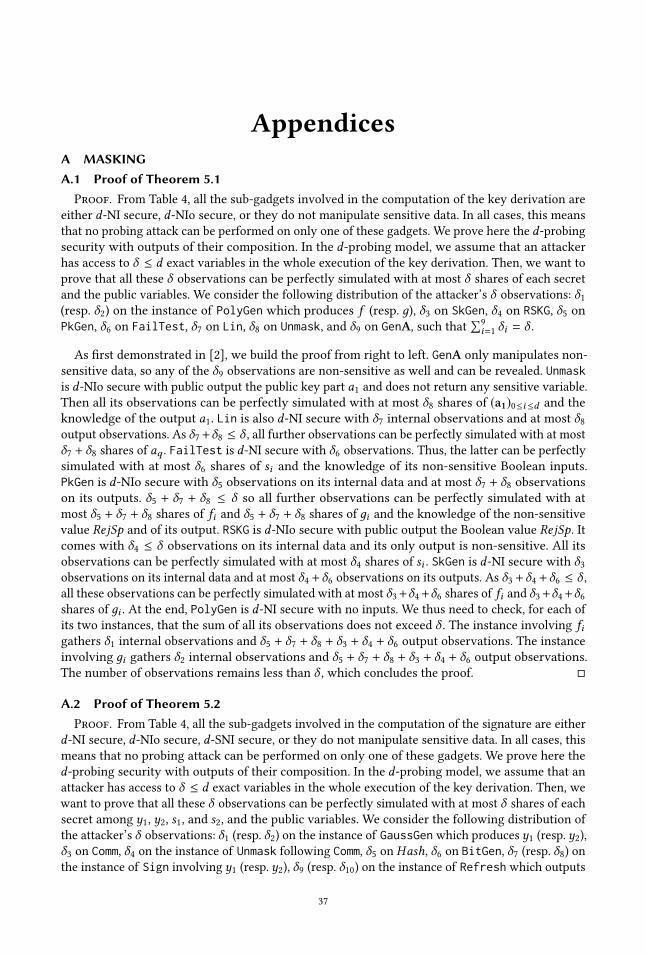
AppendicesA MASKINGA.1 Proof of Theorem 5.1

Proof. From Table 4, all the sub-gadgets involved in the computation of the key derivation are

either d-NI secure, d-NIo secure, or they do not manipulate sensitive data. In all cases, this means

that no probing attack can be performed on only one of these gadgets. We prove here the d-probingsecurity with outputs of their composition. In the d-probing model, we assume that an attacker

has access to δ ≤ d exact variables in the whole execution of the key derivation. Then, we want to

prove that all these δ observations can be perfectly simulated with at most δ shares of each secret

and the public variables. We consider the following distribution of the attacker’s δ observations: δ1(resp. δ2) on the instance of PolyGen which produces f (resp. д), δ3 on SkGen, δ4 on RSKG, δ5 onPkGen, δ6 on FailTest, δ7 on Lin, δ8 on Unmask, and δ9 on GenA, such that

∑9

i=1 δi = δ .

As first demonstrated in [2], we build the proof from right to left. GenA only manipulates non-

sensitive data, so any of the δ9 observations are non-sensitive as well and can be revealed. Unmaskis d-NIo secure with public output the public key part a1 and does not return any sensitive variable.

Then all its observations can be perfectly simulated with at most δ8 shares of (a1)0≤i≤d and the

knowledge of the output a1. Lin is also d-NI secure with δ7 internal observations and at most δ8output observations. As δ7+δ8 ≤ δ , all further observations can be perfectly simulated with at most

δ7 + δ8 shares of aq . FailTest is d-NI secure with δ6 observations. Thus, the latter can be perfectly

simulated with at most δ6 shares of si and the knowledge of its non-sensitive Boolean inputs.

PkGen is d-NIo secure with δ5 observations on its internal data and at most δ7 + δ8 observationson its outputs. δ5 + δ7 + δ8 ≤ δ so all further observations can be perfectly simulated with at

most δ5 + δ7 + δ8 shares of fi and δ5 + δ7 + δ8 shares of дi and the knowledge of the non-sensitive

value RejSp and of its output. RSKG is d-NIo secure with public output the Boolean value RejSp. Itcomes with δ4 ≤ δ observations on its internal data and its only output is non-sensitive. All its

observations can be perfectly simulated with at most δ4 shares of si . SkGen is d-NI secure with δ3observations on its internal data and at most δ4 +δ6 observations on its outputs. As δ3 +δ4 +δ6 ≤ δ ,all these observations can be perfectly simulated with at most δ3+δ4+δ6 shares of fi and δ3+δ4+δ6shares of дi . At the end, PolyGen is d-NI secure with no inputs. We thus need to check, for each of

its two instances, that the sum of all its observations does not exceed δ . The instance involving figathers δ1 internal observations and δ5 + δ7 + δ8 + δ3 + δ4 + δ6 output observations. The instanceinvolving дi gathers δ2 internal observations and δ5 + δ7 + δ8 + δ3 + δ4 + δ6 output observations.The number of observations remains less than δ , which concludes the proof. □

A.2 Proof of Theorem 5.2Proof. From Table 4, all the sub-gadgets involved in the computation of the signature are either

d-NI secure, d-NIo secure, d-SNI secure, or they do not manipulate sensitive data. In all cases, this

means that no probing attack can be performed on only one of these gadgets. We prove here the

d-probing security with outputs of their composition. In the d-probing model, we assume that an

attacker has access to δ ≤ d exact variables in the whole execution of the key derivation. Then, we

want to prove that all these δ observations can be perfectly simulated with at most δ shares of each

secret among y1, y2, s1, and s2, and the public variables. We consider the following distribution of

the attacker’s δ observations: δ1 (resp. δ2) on the instance of GaussGenwhich produces y1 (resp. y2),δ3 on Comm, δ4 on the instance of Unmask following Comm, δ5 on Hash, δ6 on BitGen, δ7 (resp. δ8) onthe instance of Sign involving y1 (resp. y2), δ9 (resp. δ10) on the instance of Refresh which outputs

37

z1 (resp. z2), δ11 on RS, δ12 (resp. δ13 and δ14) on the instance of FailTest involving c (resp. z1 andz2), and δ15 (resp. δ16) on the instance of Unmask involving z1 (resp. z2), such that

∑16

i=1 δi = δ .

We build the proof from right to left. Unmask is d-NIo secure with public output both part of

the signature z1 and z2. As a consequence, all the observations from its call involving z1 (resp z2)can be perfectly simulated with at most δ15 ≤ δ shares of z1 (resp. at most δ16 ≤ δ shares of z2)and the knowledge of the signature part z1 (resp z2). The algorithm referred to as FailTest is

also d-NI secure. Thus, all the observations from its call involving z1 (resp z2) can be perfectly

simulated with at most δ13 + δ15 ≤ δ shares of z1 (resp. at most δ14 + δ16 ≤ δ shares of z2) andthe bit RejSp which is public information indicating whether or not the rejection sampling failed.

The third instance of FailTest involving c does not manipulate any sensitive data and can be

safely left unmasked. Then, RS is d-NIo secure with public output RejSp and does not return any

sensitive element. All the observations performed in this gadget and its output can be perfectly

simulated with at most δ11 shares of each input among s1, s2, z1, z2, the knowledge of c , which is

here public, and the knowledge of RejSp. Continuing from right to left, we consider both instances

of Refresh. From its d-SNI security property and since the output and local observations are still

less than δ , all observations from its call can be perfectly simulated with at most δ9 ≤ δ (resp.

δ10 ≤ δ ) input shares. Both instances of Sign outputs variables that are immediately refreshed.

Sign is additionally d-NI secure and has δ9 (resp. δ10) output observations and δ7 (resp. δ8) internalones. In both cases the addition of the internal and output observations remains below δ and the

d-NI property makes it possible to simulate all further observations with δ7 + δ9 ≤ δ shares of

y1,i , s1,i , bi , and the knowledge of c (resp. δ8 + δ10 ≤ δ shares of y2,i , s2,i , bi , and the knowledge

of c). BitGen is d-NI secure and since it has no inputs, the fact that the δ7 + δ9 + δ8 + δ10 ≤ δoutput observations and δ6 internal observations are less than δ is enough to guarantee the global

security from its location. Hash only manipulates public data. Unmask is d-NIo secure and does not

return any sensitive variable. Then all the observations performed from this gadget can be perfectly

simulated with at most δ4 shares of ui . Comm is d-NI secure. δ3 observations are performed on its

intermediate variables, and at most δ4 observations are performed on its outputs. As δ3 +δ4 ≤ δ , allfurther observations can be perfectly simulated with at most δ3+δ4 shares of y1, δ3+δ4 shares of y2and the knowledge of the public value A. The last step of the proof is to verify that all the internal

and output observations on each instance of GaussGen are less than δ . Internal observations arerespectively δ1 and δ2 while output observations are bounded by δ3+δ4+δ7+δ9 and δ3+δ4+δ8+δ10which are both less than δ . The d-NIo property of GaussGen concludes the proof. □

B PROOFSB.1 Proof of Corollary 4.2

Proof. Let us suppose that

���D−D′D

��� ≤ 2−45

is verified. Then, 1 − 2−45 ≤ D′

D≤ 1 + 2

−45. Since

Supp(D ′) = Supp(D), we apply the relative error Lemma (Lemma 3 of [35]), and get

R2·λ(D||D′) ≤ 1 + 2·λ ·2−2·45

2

≤ 1 + 256 · 2−2·45

≤ 1 + 2−82

= 1 + 1

4qD.

This corresponds to Equation 2 and completes the proof.

□

38

B.2 Proof of Lemma 4.5Proof. Let x0 ∈ I be such that |u(x)| ≥ |u(x0)| for all x ∈ I . We then write

u(x) = u(x0) +

∫ x

x0u ′

Hence,

|u(x)| ≤ |u(x0)| +

∫ x

x0|u ′ | ≤

1

|I |

∫I|u | +

∫I|u ′ |

Using Cauchy-Schwarz, we have

( ∫I |u |

)2

≤ |I |∫I |u |

2and

( ∫I |u′ |)2

≤ |I |∫I |u′ |2. Then,

|u(x)| ≤1

|I |

√|I |

∫I|u |2 +

√|I |

∫I|u ′ |2

Using the equality x + y ≤√2

√x2 + y2 for x ,y ≥ 0, we have

|u(x)| ≤√2

√1

|I |2· |I |

∫I|u |2 + |I |

∫I|u ′ |2

Then,

| |u | |∞ ≤√2 · |u |

S

which concludes the proof. □

B.3 Proof of Lemma 4.6Proof. By hypothesis,

∀t ∈ I3|P I3

exp(t) − exp

(t

2σ 2

)|

| exp

(t

2σ 2

)|

≤

������P I3exp − exp(

.2σ 2

)exp

(.

2σ 2

) ������∞≤ 2−K

39

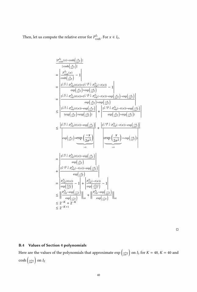
Then, let us compute the relative error for P I2cosh

. For x ∈ I2,

|P I2cosh(x )−cosh

(x

2σ 2

)|

| cosh

(x

2σ 2

)|

=

����� P I2cosh(x )

cosh

(x

2σ 2

) − 1�����

=

����� 2 ⌊ xc ⌋ ·P I3exp(t (x ))+2 ⌊ −xc ⌋ ·P I3exp(−t (x ))exp

(x

2σ 2

)+exp

(−x2σ 2

) − 1

�����=

����� 2 ⌊ xc ⌋ ·P I3exp(t (x ))+2 ⌊ −xc ⌋ ·P I3exp(−t (x ))−exp(

x2σ 2

)−exp

(−x2σ 2

)exp

(x

2σ 2

)+exp

(−x2σ 2

)�����

≤

����� 2 ⌊ xc ⌋ ·P I3exp(t (x ))−exp(

x2σ 2

)(exp

(x

2σ 2

)+exp

(−x2σ 2

))

����� +����� 2 ⌊ −xc ⌋ ·P I3exp(−t (x ))−exp

(−x2σ 2

)exp

(x

2σ 2

)+exp

(−x2σ 2

))

�����≤

���2 ⌊ xc ⌋ ·P I3exp(t (x ))−exp( x2σ 2

)��������������exp

(x

2σ 2

)+exp

(−x

2σ 2

)︸ ︷︷ ︸

>0

�����������

+

���2 ⌊ −xc ⌋ ·P I3exp(−t (x ))−exp( −x2σ 2

)��������������(exp

( x

2σ 2

)︸ ︷︷ ︸

>0

+ exp(−x2σ 2

))

�����������=

����� 2 ⌊ xc ⌋ ·P I3exp(t (x ))−exp(

x2σ 2

)exp

(x

2σ 2

)�����

+

����� 2 ⌊ −xc ⌋ ·P I3exp(−t (x ))−exp(−x2σ 2

)exp

(−x2σ 2

)�����

=

����� P I3exp(t (x ))exp

(t (x )2σ 2

) − 1����� +

����� P I3exp(−t (x ))exp

(−t (x )2σ 2

) − 1�����

≤

������ P I3exp−exp( .2σ 2

)exp

(.

2σ 2

) ������∞+

������ P I3exp−exp( .2σ 2

)exp

(.

2σ 2

) ������∞

≤ 2−K + 2−K

≤ 2−K+1

□

B.4 Values of Section 4 polynomials

Here are the values of the polynomials that approximate exp

(.

2σ 2

)on I3 for K = 48, K = 40 and

cosh

(.

2σ 2

)on I2

40

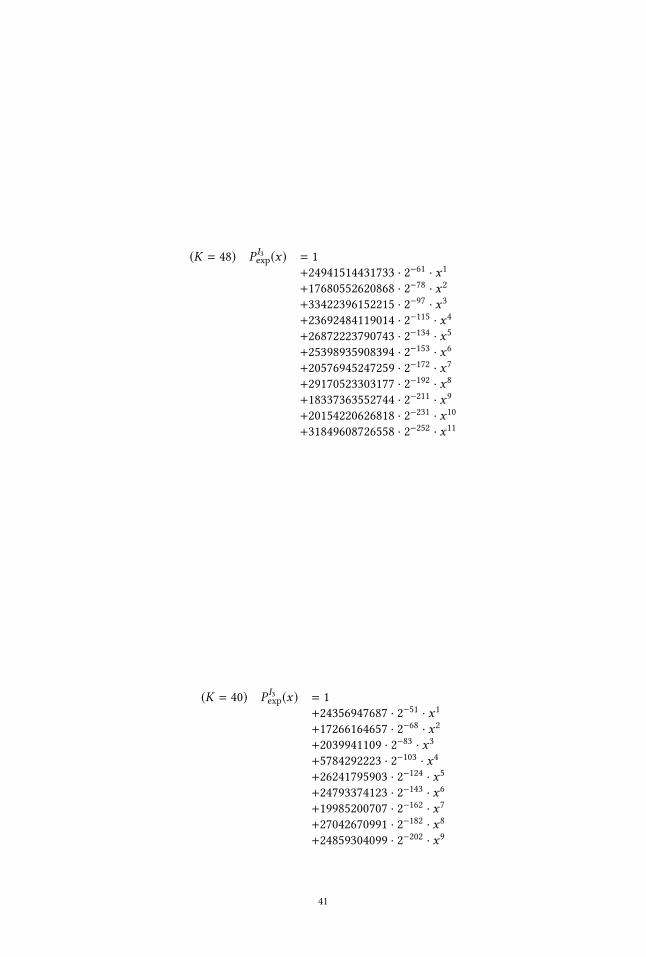
(K = 48) P I3exp(x) = 1

+24941514431733 · 2−61 · x1

+17680552620868 · 2−78 · x2

+33422396152215 · 2−97 · x3

+23692484119014 · 2−115 · x4

+26872223790743 · 2−134 · x5

+25398935908394 · 2−153 · x6

+20576945247259 · 2−172 · x7

+29170523303177 · 2−192 · x8

+18337363552744 · 2−211 · x9

+20154220626818 · 2−231 · x10

+31849608726558 · 2−252 · x11

(K = 40) P I3exp(x) = 1

+24356947687 · 2−51 · x1

+17266164657 · 2−68 · x2

+2039941109 · 2−83 · x3

+5784292223 · 2−103 · x4

+26241795903 · 2−124 · x5

+24793374123 · 2−143 · x6

+19985200707 · 2−162 · x7

+27042670991 · 2−182 · x8

+24859304099 · 2−202 · x9

41

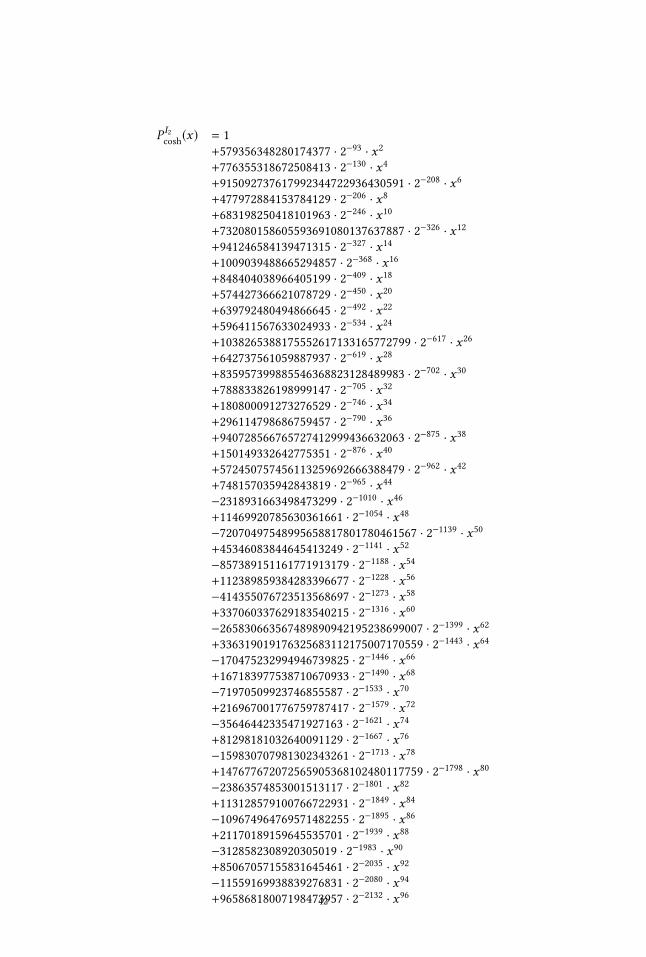
P I2cosh(x) = 1

+579356348280174377 · 2−93 · x2

+776355318672508413 · 2−130 · x4

+915092737617992344722936430591 · 2−208 · x6

+477972884153784129 · 2−206 · x8

+683198250418101963 · 2−246 · x10

+732080158605593691080137637887 · 2−326 · x12

+941246584139471315 · 2−327 · x14

+1009039488665294857 · 2−368 · x16

+848404038966405199 · 2−409 · x18

+574427366621078729 · 2−450 · x20

+639792480494866645 · 2−492 · x22

+596411567633024933 · 2−534 · x24

+1038265388175552617133165772799 · 2−617 · x26

+642737561059887937 · 2−619 · x28

+835957399885546368823128489983 · 2−702 · x30

+788833826198999147 · 2−705 · x32

+180800091273276529 · 2−746 · x34

+296114798686759457 · 2−790 · x36

+940728566765727412999436632063 · 2−875 · x38

+150149332642775351 · 2−876 · x40

+572450757456113259692666388479 · 2−962 · x42

+748157035942843819 · 2−965 · x44

−2318931663498473299 · 2−1010 · x46

+11469920785630361661 · 2−1054 · x48

−72070497548995658817801780461567 · 2−1139 · x50

+45346083844645413249 · 2−1141 · x52

−857389151161771913179 · 2−1188 · x54

+112389859384283396677 · 2−1228 · x56

−414355076723513568697 · 2−1273 · x58

+337060337629183540215 · 2−1316 · x60

−265830663567489890942195238699007 · 2−1399 · x62

+336319019176325683112175007170559 · 2−1443 · x64

−170475232994946739825 · 2−1446 · x66

+167183977538710670933 · 2−1490 · x68

−71970509923746855587 · 2−1533 · x70

+216967001776759787417 · 2−1579 · x72

−35646442335471927163 · 2−1621 · x74

+81298181032640091129 · 2−1667 · x76

−159830707981302343261 · 2−1713 · x78

+147677672072565905368102480117759 · 2−1798 · x80

−23863574853001513117 · 2−1801 · x82

+113128579100766722931 · 2−1849 · x84

−109674964769571482255 · 2−1895 · x86

+21170189159645535701 · 2−1939 · x88

−3128582308920305019 · 2−1983 · x90

+85067057155831645461 · 2−2035 · x92

−11559169938839276831 · 2−2080 · x94

+96586818007198473957 · 2−2132 · x9642