IADC/SPE 27499

Gas Rises Rapidly Through Drilling MudJ.A. Tarvin,* Schiumberger-Doll Research; A.P. Hamilton, Schlumberger CambridgeResearch; P.J. Gaynord, Anadrill Schlumberger; and G.D. Lindsay, Sedco ForexSchlumberger

'SPE MemberlADe Members

Copyright 1994, IADC/SPE Drilling Conference.

This paper was prepared for presentation at the 1994 IADC/SPE Drilling Conference held in Dallas, Texas, 15-18 February 1994.

This paper was selected for presentation by an IADC/SPE Program Committee following review of inform~lion contai.n?d in an abstract submitted ~y the author(~). Contents of the paper,as presented, have not been reviewed by the Society of Petroleum Engineers or the International AssociatIon of Dniling Contractors and are subject to correction by the author(s). Thematerial, as presented, does not necessarily reflect any position of the IADC or SPE, their officers, or members. Papers presented at IADC/SPE meetings are subject to publicationreview by Editorial Committees of the IADC and SPE. Permission to copy is restricted to an abstract of not more than 300 wo!ds. illustrations may not be copIed. The abstract shouldcontain conspicuous acknowledgment of where and by whom the paper is presented. Write Librarian, SPE, P.O. Box 833836, Richardson, TX 75083·3836, U.S.A. Telex, 163245 SPEUT.

ABSTRACTTo understand the development of a gas kick, we mustknow the rate at which gas migrates upward throughdrilling mud. Migration rates measured in laboratoryexperiments are much greater than those commonly ac­cepted by the drilling industry. To address this con­troversy, we use a computer simulator to model fielddata and test-well experiments in detail. Both the ex­periments and the field data show that gas migrates asfast as 6000 ftlhr [0.5 m/s] through drilling mud. Thefield data show that gas migration can drive surfacepressure up as fast as 3000 psilhr [4.9 kPals]. Theseconclusions agree with laboratory experiments andcontradict what is generally accepted in the industry.

The results from the simulation of the field kickwere incorporated in a case study. The study increasesdrill crew awareness of the speed at which gas can ar­rive at surface and demonstrates that a reduction inpump pressure can be a very late kick indicator.

1. INTRODUCTIONFluid that enters a well during drilling poses a dangerto the well, the drilling rig, the environment and thecrew. Gas kicks are particularly dangerous becausegas reduces wellbore pressure more quickly than liq­uids do and because gas is more difficult to confine atthe surface. Thus, gas kicks more often result in lossof well control and in surface fires and explosions.

References and illustrations at end of paper.

637

Many mathematical models, or simulators, havebeen developed to improve detection and control of gaskicks. Past work has recently been reviewed. l Thesesimulators require models of many physical processesin the wellbore. One of the most important of thoseprocesses is the buoyant migration of gas throughdrilling mud. Gas migration modifies the pressuredistribution throughout the well during a kick and itdetermines the time when gas first reaches the surface.

It is widely believed in the drilling industry thatgas rises through drilling mud at 1000 ftlhr [8 cm/s] orslower, and even as slowly as 200 ftlhr [1.7 cm/s].2Consequently, it is generally accepted that gasmigration, on its own, cannot cause surface pressuresto rise faster than a few hundred psi per hour. On theother hand, a variety of laboratory3-6 and test-we1l3,7experiments indicate that gas moves as fast as 6000ftlhr. As a result, there should be some cases whengas migration drives pressure up at thousands of psiper hour. One would think that any (or all) fiel~ datacould distinguish between these rates; but such IS notthe case. The volume and composition of an influx areoften uncertain; and poorly understood processes, suchas loss of fluid to permeable formations or deformationof weak formations, also complicate the interpretation.

To resolve this controversy, we must first realizethat the experimeIits generally refer to gas volume fr~c­

tions exceeding several percent When the gas fracoonis 1% to 2%, or less, experiments show that gasmoves slowly. More important is the fact that gas mi-

(1)

(2)Mud pumped + Pit Gainv - --:...---=------

m - Time . Area .

where Vm is the velocity of the mud just above the gasand Co is a distribution factor. Co is 1.0 for the indus­try model and 1.35 for the SCR correlation. The slipvelocity, vs, is 0.085 rnJs [1000 ft/hr] for the industrymodel; it depends on geometry in the SCR correlation,as shown in Table 2. Notice that these slip velocitiesare even greater than 0.5 m/s because the wellbore ismore than 12 inches in diameter. It remains to estimateVm from the pit gain and the flow into the well:

Note that Eq. (2) is an average from the start ofthe kick to the arrival of gas at the surface. The totalmud pumped during the kick was 16.4 m3. The mea­sured pit gain, relative to the pit level during the con­nection, was 17.8 m3. Since some mud was blownout of the well and not returned to the pits, the totalquantity of mud expelled from the well was greater

2 GAS RISES RAPIDLY THROUGH DRILLING MUD SPE 27499

gration can seldom be determined directly from field the connection at 0 time, the flow out of the well wasdata. Instead, gas migration rates are generally in- stable for at least 20 minutes. Since the kill mud sta-ferred from the rate of change of surface pressure. bilized the well, we estimate that the formation poreJohnson et at.8,6 have shown that mud compressibil- pressure was equivalent to a mud density of 1320ity, fluid loss and wellbore compliance modify surface kglm3. Since the pit level and flow out increased sopressures substantially. Since the standard interpreta- rapidly, the producing formation had a high effectivetion for surface pressures ignores these effects, it is permeability. Although the pore pressure was 290 psiusually invalid. [2 MPa] greater than wellbore pressure, Figure 1

In this paper, we present additional evidence that shows no flow out of the well during the connection.gas rises rapidly through drilling mud. Since gas eas- Therefore, the producing formation was entered afterily dissolves in oil-base mud (OBM), it usually mi- the connection and only a small quantity of gas couldgrates slowly in OBM. The data and analysis pre- have been swabbed into the well during the connec-sented here apply specifically to water-base mud tion. Mter drilling restarted, the flow into the well (not(WBM). The evidence includes a field case and simu- shown) reached 33 Us at 9 minutes and the flow outlations of both field data and test-well experiments. was the same at this time. However, the flow out in-Section 2 shows a field case that demonstrates directly creased by 10 Us in the next 90 seconds. Therefore,that gas migrates as fast as laboratory experiments in- the influx started at 9.5±1 minutes.dicate. Section 3 discusses our simulation tools and The driller's report indicates that gas reached themethods. Section 4 gives results of the field case surface by the time the BOP closed at 24 minutes. Gassimulations and describes the use of the simulations in in the riser (above the BOP) continued to blow mudwell-control training. Section 5 presents the results of out of the well for some time. The time required forsimulations of the test-well experiments. gas to travel the 1350 m up the well was, therefore,

14.5 minutes; and the average gas velocity Vg was1.55 mls [18300 ft/hr].

We now compare the observed gas velocity witha correlation based on laboratory data4 fromSchlumberger Cambridge Research ("SCR correla­tion") and with the 1ooo-ft/hr rule of thumb generallyaccepted in the drilling industry. For either model, thevelocity of the uppermost portion of the gas is

2. GAS VELOCITY FROM A FIELD CASEThe field case occurred on a rig drilling in 120 m ofwater on the Mrican coast. The well was vertical withthe geometry given in Table 2 and the mud density was1170 kg/m3 [9.8 Ibm/gal]. Shortly after a connection,both the flow out of the well and the pit level increasedrapidly, as in Figure 1. Circulation was stoppedbriefly to check whether the well was flowing and thewell was shut in just as gas reached the surface. Thepit gain was 107 bbl [17 m3], with respect to the pitlevel measured during the preceding connection. Somemud was lost as gas blew it out of the drilling riserafter the blow-out preventer (BOP) closed. The wellwas eventually brought under control with a kill muddensity of 11.3 Ibm/gal [1350 kg/m3].

This field case is ideal for testing gas migrationmodels, because both the start of the influx and thetime of arrival of gas at the surface can be determinedaccurately and because the, kick lacks many of the fea­tures that complicate the interpretation of most kicks.From the timing of the kick, we can estimate the aver­age gas velocity and compare it with predictions of gasmigration models. Since the casing shoe was only 89m above the bottom during the kick, wellbore defor­mation and fluid loss had minimal effect on the surfacepressure. In this section, we show that the time forgas to reach the surface in this kick is consistent withlaboratory measurements and is entirely inconsistentwith a standard field model for gas migration.

We can identify the start of the influx from the pitgain and the flow out of the well in Figure 1. Before

638

4. FIELD CASE SIMULATIONThe geometry of the well and the drillstring are givenin Table 2. The drilling-mud and formation physicalproperties are given in Table 3. The pore pressure ofthe producing formation is estimated from the fmal killmud density used in the successful kill operation.Since the formation porosity isn't known, it was set at15%; it has only a minor effect on the simulations.

The purpose of this modeling exercise is to simu­late closely the development of a kick and its shut-inperiod, using the SideKick simulator with its experi­mentally derived gas rise correlation. Since this corre­lation predicts rapidly moving gas, we refer to. thissimulation as "Fast Gas." For the sake of companson,we repeat the simulation, with the simulator modifiedto use the industry standard figure for gas rise of1,000 ft/hr. The second simulation is called "Slow

Thus, the SCR correlation gives a gas velocity of1.48 mls and the industry model gives 0.72 m/s.When compared with the observed velocity of 1.55mis, the SCR correlation is obviously much better thanthe industry model.

3. SIMULATION METHODSTo simulate the field case and the experiments, weused the SideKick9 gas kick simulator. The technicalcontent of this simulator has been described previ­ously)O It has been used to analyze field casesll andto aid well planning.12 Status data required for a simu­lation include the well geometry and trajectory andphysical properties of the mud and the producing for­mation.

The model has four boundary conditions: inletand outlet flow rate and inlet and outlet pressure. Ateach time, the user specifies two of these conditions.In some cases, the pressure or flow rate can be speci­fied at an interior point instead of a boundary. Thesimulator then computes the flow rates and pressuresthroughout the well, including the boundary conditionsnot specified by the user. For most simulations, thespecified boundary conditions are the outlet pressure(one atmosphere) and the measured inlet flow rate.When the well is shut in, the specified boundary con­ditions are the inlet and outlet flow rates (both zero).

(3)34.2 m3

v = 2 =0.63 m Is.m 870 s . 0.0624 m

SPE 27499 I.A. Tarvin, A. Hamilton, P. Gaynord and G.Lindsay 3

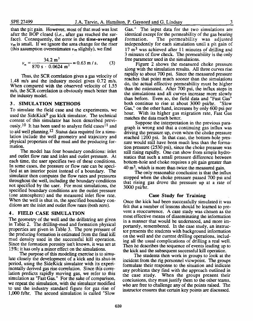
than the pit gain. However, most of that mud was lost ~as. ': The input data for the. ~wo simulations ~re

after the BOP closed (i.e., after gas reached the sur- Idenuca! except for the permeab~l~ty of the gas b.earmgface). Consequently, the error in the time.avera~ed ~ormatlOn. The pe~meab~hty ~as .adJu.stedVm is small. If we ignore the area change for the nser mdependently for each sImulatIon unul a pIt gam of(this assumption overestimates Vm slightly), we find 17 m3 was achieved after 11 minutes .o! d~lling and

3 minutes of flow check. The permeabIhty IS the onlyfree parameter used in the simulations.

Figure 2 shows the measured choke press~re

along with the simulation results. All three curves nserapidly to about 700 psi. Since the measured pressurereaches that point much sooner than the simulationsdo, the actual effective permeability must be higherthan the estimated. Mter 700 psi, the influx stops inthe simulations and all curves increase more slowlythan before. Even so, the field data and "Fast Gas"both continue to rise at about 3000 psi/hr. "SlowGas," on the other hand, increases by only 600 psi perhour. With its higher gas migration rate, Fast Gasmatches the data much better.

Suppose the interpretation in the previous para­graph is wrong and that a continuing gas influx wasdriving the pressure up, even when the choke pressurereached 1200 psi. In that case, the bottom-hole pres­sure would still have been much less than the forma­tion pressure (2530 psi), since the choke pressure wasstill rising rapidly. One can show from simple hydro­statics that such a small pressure difference betweenbottom-hole and choke requires a pit gain greater than40 m3, which is more than twice the measured gain.

The only reasonable conclusion is that the influxstopped when the choke pressure passed 700 psi andthat rising gas drove the pressure up at a rate of3000 psi/hr.

Case Study for TrainingOnce the kick had been successfully simulated it wasfelt that a number of lessons should be learned to pre­vent a reoccurrence. A case study was chosen as themost effective means of disseminating the informationin a manner that would be understood, and more im­portantly, remembered. In the case study, an instruc­tor presents the students with background informationon the well and the current drilling operations, includ­ing all the usual complications of drilling a real well.Then he describes the sequence of events leading up tothe kick and the subsequent successful kill operation.

The students then work in groups to look at theincident from the rig personnel viewpoint. The groupsformulate their response to the situation and indicateany problems they find with the approach outlined ~n

the case study. When the groups present theIrconclusions, they must justify them to the other teams,who are free to challenge any of the points raised. Theinstructor ensures that certain key points are discussed.

639

4 GAS RISES RAPIDLY THROUGH DRILLING MUD SPE 27499

The instructor then presents a summary of theincident with the benefit of the simulation results. Thefirst thing the students are shown is a video recordingof the real-time simulation screen. This clearly showsthe surface indicators such as the pit gain and standpipepressure along with a picture of the correspondingdownhole situation during the drilling phase. Theprimary use of the simulation is to visually reinforcethe points covered during the classroom discussion.

The students can see, for example, that the wellis kicking while the driller has the pumps stopped toinvestigate the loss in standpipe pressure. The drillerhad previously asked his assistant about an increase inpit gain but was told that a mud transfer was beingcarried out. He was not informed when the transferwas complete. He had had previous problems withwashouts and assumed this was another one. As inmany of these situations, it is a combination of eventsthat lead to the kick remaining undetected for so long.The students can identify many ways to break thischain of events. They can also see that by the time akick has caused noticeable decrease in standpipe pres­sure it is already well developed.

Another item covered is the change in maximumallowable annular surface pressure (MAASP) causedby the combination of gas displacement during drillingand its migration after the well has been shut in. Therewas some concern at the rig site that the choke pressurewas exceeding the MAASP immediately after the wellwas shut in. The students can see on the simulationthat a large amount of gas is above the casing shoe atshut-in and that this continues to increase as the gasrises. The reduced hydrostatic pressure above thecasing shoe allows a greater choke pressure before theshoe reaches its breakdown pressure. Figure 3 showsthat the MAASP increased by 50% during the kick.Consequently, the choke pressure could increase to400 psi above the pre-kick MAASP before there wasdanger of formation breakdown.

The use of the simulation helps improve thestudents' understanding of downhole events and howthey relate to what is seen at surface. It also helpsreinforce the ideas covered in the group discussion.

S . TEST·WELL EXPERIMENTSThe test-well data come from the well-control experi­ments performed at Rogalands Research Institute l3 ,where nitrogen gas was injected into a 15OO-m deep,cased well. The experiments were performed withboth OBM and WBM. Since the OBM experimentswere done first, the WBM contained some oil. Severalmeasurements showed that the oil fraction wasbetween 2% and 4% by volume. Since there is noreason why the oil fraction should have varied, weattribute the fluctuation to measurement errors and set

640

the fraction to 3% for all simulations. This smallquantity of oil changed the nitrogen solubility of themud significantly and affected all simulations.

The gas was injected through coiled tubing in­serted inside the drillstring to the bottom of the well.Several injection procedures were used. In the bestmethod, the desired quantity of nitrogen was injectedinto the tubing as a single slug, with plugs on each endto keep the gas separated from the mud in the tubing.More mud was then pumped into the tubing to displacethe gas into the annulus. The pressure at the tubinghead was held nearly constant during the gasdisplacement. .

We have analyzed four WBM experiments thatused this injection method, because the start and end ofinjection are clear. Each of the four experiments in­volved a different procedure after the gas injection.

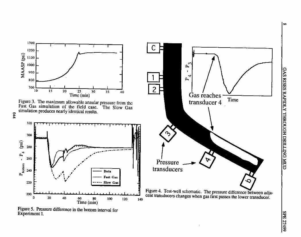
The key data from these experiments are the si­multaneous pressure measurements at six depths in theannulus. The pressure difference between adjacenttransducers changes abruptly when gas first enters theinterval between them. Thus, plots of pressure differ­ences are direct indicators of gas migration. Figure 4shows a schematic drawing of the wellbore and a typi­cal curve for the pressure difference. The depths of thesix pressure transducers, with respect to the kellybushing, are given in the Table 4 for each of the fourexperiments. Since the choke is above the kelly bush­ing, its depth is negative.

To see the effects of the gas-migration relation,we have simulated the experiments two ways withSideKick. First, we used the standard gas-slip rela­tion, which includes both a slip velocity and a distribu­tion factor. The slip relation is derived from laboratoryexperiments6 and includes the effects of the well ge­ometry and trajectory. The parameters in the relationhave not been modified to match these experiments. Atypical slip velocity for these experimental conditions isabout 0.55 mls [6500 ftlhr]. Curves derived from thiscomputation are labeled "Fast Gas." Second, we useda typical industry estimate of 0.085 mls [1000 ftlhr] forthe slip velocity. Curves derived from that computa­tion are labeled "Slow Gas. "

Experiment IThis is the largest of the four kicks, with 400 kg[880 Ibm] of gas injected. At bottom-hole conditions,the gas would displace 15.7 bbl [2.5 m3]of mud. Atthe start of injection, the gas filled the whole coiledtubing string. At a given flow rate, the frictionalpressure for mud is much higher than for gas. Sincethe pump pressure was nearly constant duringinjection, the flow rate into. the well decreasedsignificantly as mud displaced gas in the tubing.Therefore, the gas injection rate was much higher than

SPE 27499 I.A. Tarvin. A. Hamilton. P. Gaynord and G. Lindsay 5

the average, initially. The measured flow rate out ofthe well confinns this change. In the simulations, wehave used an injection rate that starts at 1.1 kg/s andthen rapidly decreases to 0.2 kg/so

Figure 5 shows the pressure difference Pb - P4for Experiment I. All three curves drop sharply at 17minutes when injection starts. The curves level off ortum upward when gas reaches P4. This event occursat 24 minutes in the data and 23 minutes in the standardSideKick ("Fast Gas") model. The Slow Gas model isseveral minutes late. All the curves have jumps at 39minutes when injection ended and the well was shut in.These jumps result from changes in frictional pressurethat occur when the flow rate changes abruptly.

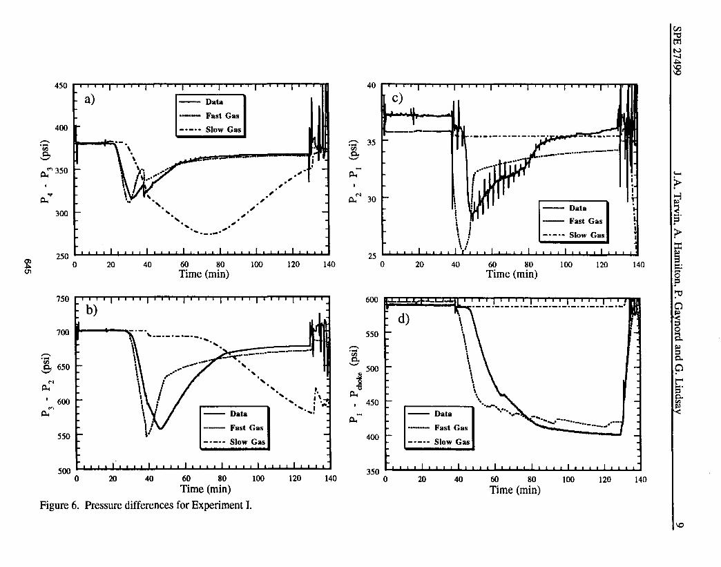
Figure 6 shows the pressure differences in thenext four intervals of the well. The Slow Gas simula­tion is obviously incorrect It has the gas arriving sev­eral minutes late in the P4 - P3 interval and 30 minuteslate in the P3 - P2 interval. The gas does not reach theP2 - PI and PI - Pchoke intervals until circulation startsagain at 130 minutes. The data clearly disagree withthis simulation. On the other hand, the Fast Gas simu­lation has gas arriving within a few minutes of the cor­rect time in all intervals.

Preliminary simulations of this experimentS ig­nored the oil content of the mud and used a gas migra­tion relation based on earlier experiments.4 Thus, theresults shown here differ somewhat from the prelimi­nary ones; but the conclusions are the same.

Experiment IIIn this and subsequent experiments, approximately 141kg [310 Ibm] of gas were injected. That much gaswould displace about 5.5 bbl [0.9 m3] of mud atbottom-hole conditions. Since most of the coiledtubing was filled with mud at the start of injection, theinjection rate was nearly constant. Therefore, theinjection rate was held constant during the simulationsfor Experiments II to N.

In this experiment, circulation stopped when theinjection finished and the gas rose into nearly staticmud. Since the gas mass was relatively small, itspread out over most of the depth of the well. As a re­sult, the gas concentration was small everywhere andthe simulations are very sensitive to the oil concentra­tion, which has a relatively high uncertainty.

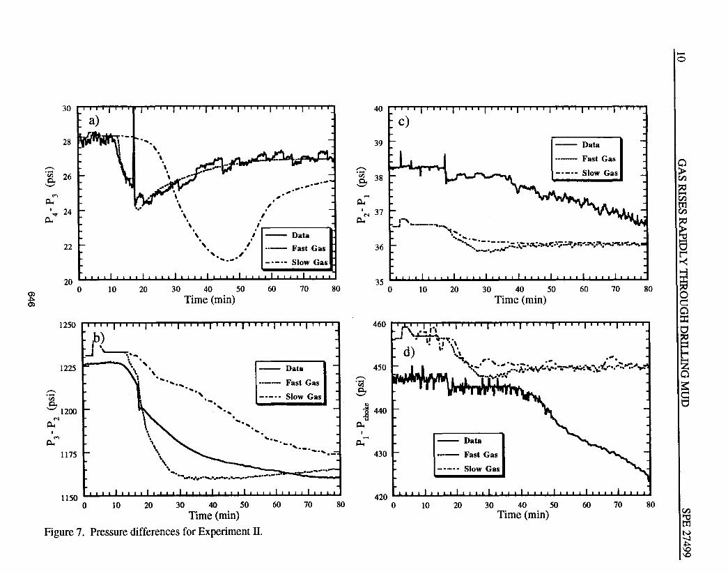
Figure 7 shows the data and simulations for ex­periment II. Gas injection started at 5 minutes andended at 17 minutes. The data show that gas reachedthe P4 - P3 interval at 11 minutes and the PI - Pchokeinterval at about 40 minutes. The gas traveled the 922m interval from P4 to PI in 29 minutes. The averagevelocity was therefore 0.53 mls. However. during thefirst six minutes, mud flowed into the well at 39gal/min and gas was injected at 25 gal/min. Correcting

641

for these flows, we find an average velocity of 0.50mls for the gas relative to the mud. T\1is is six timesthe typical industry estimate, but it is only 10% lessthan the laboratory experiments indicate, even thoughthe gas volume fraction was only a few percent.

Although the Fast Gas simulation is better, nei­ther simulation agrees well with all the data in this ex­periment. .The Fast Gas simulation accurately repro­duces the pressure difference in the P4 - P3 interval,and it has gas arriving in the P3 - P2 interval at the cor­rect time. Slow Gas is 10 minutes late in the P4 - P3interval. It is equally late in the P3 - P2 interval, al­though the figure doesn't show it clearly. Both simu­lations have gradual changes in differential pressurebetween 17 and 30 minutes because the mud flow ratewas decreased during that period. All the computedpressure changes in the P2 - PI and PI - Pchoke inter­vals result from small changes of mud flow. Thus,both simulations fail to reproduce the early arrival ofgas in the upper portion of the well.

It is clear that Slow Gas could never simulate theearly gas arrival. but why doesn't Fast Gas do better?The reason is the relatively low gas concentrationthroughout the well. The uncertainty in the oil fractionresults in a large relative uncertainty in the free gasfraction. In the Fast Gas simulation, the free gas frac­tion falls below the minimum required for the gas tomove rapidly. It would be possible to match the databetter if the oil fraction were reduced in the simulation.

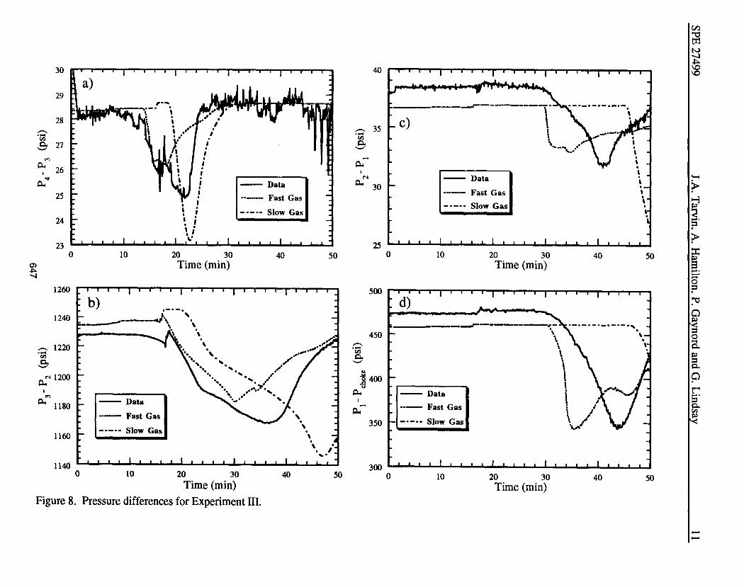
Experiment IIIIn this experiment, the circulation rate increased to 150gal/min when the injection finished. Figure 8 showsthe data and simulations. Injection started at 5 minutesand ended at 16 minutes. Fast Gas has gas arriving ineach interval within two minutes of the time indicatedby the data. However, the gas seems to fill the upperintervals too quickly. Slow Gas has gas arriving laterand later as the gas moves up the well. The computedarrival in the highest interval is 16 minutes late. Notethat the circulation reduced the length of the experimentto 45 minutes and consequently decreased the differ­ence between the simulations.

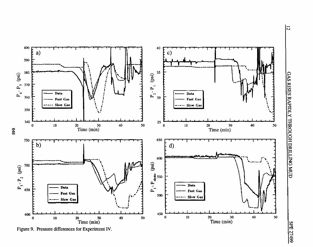
Experiment IVIn this experiment, the circulation rate increased to 320gal/min when the injection finished. Figure 9 showsthe data and simulations. Injection started at 12 min­utes and ended at 23 minutes. Significant changes ofmud flow rate occurred at 23, 36 and 44 minutes.Pressure changes at those times result from frictionalpressure and should be ignored. In the simulations ofthis experiment, the specified boundary conditionswere the inlet flow rate and the measured bottom-holepressure. Fast Gas has gas arriving in each interval

6. CONCLUSIONSA field case and four test-well experiments are all con­sistent with gas migration rates derived from laboratoryexperiments. All five comparisons show that the mi­gration rates generally accepted in the drilling industryare much too low.

If a driller believes that gas rises more slowlythan it really does, he may overestimate the casing­shoe pressure and the gas will arrive at the surfacesooner than he expects. The driller may not be pre­pared when the gas surfaces, or he may misinterpretpit-level and pressure measurements. These errors canhave serious consequences during a critical operationalprocedure.

Summary of Test-Well ExperimentsIn each of the four experiments discussed above, theFast Gas simulation is superior. If gas really doesmove fast, then why do surface pressures seem to im-ply that gas moves slowly? Johnson et al.8,6 haveshown that wellbore compliance and fluid loss reducethe rate of pressure increase. Here, we show that sur­face pressures can rise rapidly during shut-in. Figure10 shows the choke pressure in Experiment I. Duringthe first five minutes of shut-in, the measured pressureincreases at the same rate as in the Fast Gas simulation.Thereafter, the measured pressure rises somewhatmore slowly, but still far more rapidly than in the SlowGas simulation. Eventually, the pressure stopschanging because most of the gas is at the top of thewell. In the Slow Gas simulation, none of the gas hasreached the top of the well by the end of shut-in at 130minutes. There is no doubt that gas moved rapidly inthese experiments.

6 GAS RISES RAPIDLY THROUGH DRILLING MUD SPE·27499

within three minutes of the time indicated by the data. puter Models," Int. Well Control Symposium,Slow Gas has gas arriving later and later as the gas Louisiana State University, Nov. 27-29, (1989).moves up the well. The computed arrival in the high- 2. Blount, E.: "Executive Summary," SPE Drillingest interval is about 12 minutes late. Once again, the Engineering 6, (1991) 236.circulation reduced the length of the experiment anddecreased the difference between the simulations. 3. Rader, D.W., Bourgoyne, A.T. and Ward,However, it is still clear that Slow Gas is much too R.H.: "Factors Mfecting Bubble Rise Velocity ofslow. Gas Kicks," JPT (May 1975) 571-585.

4. Johnson, A.B. and White, D.B.: "Gas RiseVelocities During Kicks," SPE DrillingEngineering 6 (1991) 257.

5. Skalle, P., Podio, A.L. and Tronvoll, J.:"Experimental Study of Gas Rise Velocity and itsEffect on Bottomhole Pressure in a VerticalWell," SPE 23160 (1991).

6. Johnson, A.B. and Cooper, S.: "Gas MigrationVelocities During Gas Kicks in Deviated Wells,"SPE 26331 (1993).

7. Hovland, F. and Rommetveit, R.: "Analysis ofGas-rise Velocities from Full-scale Kick Experi­ments," SPE 24580 (1992).

8. Johnson, A.B. and Tarvin, J.A.: "Field Calcula­tions Underestimate Gas Migration Velocities,"IADC European Well Control Conf. (1993) andOil & Gas J., November 15 (1993) 55-60.

9. Hamilton, T.A.P., Swanson, B. and Wand, P.:"Use of New Kick Simulator Will IncreaseWellsite Safety," World Oil (Sept. 1992).

10. White, D.B. and Walton, I.e.: "A ComputerModel for Kicks in Water- and Oil-Based Muds,"SPE 19975, (1990).

11. Tarvin, J.A., Walton, I., Wand, P. and White,D.B.: "Analysis of a Gas Kick Taken in a DeepWell Drilled with Oil-based Mud," SPE 22560(1991).

12. Leach, C.P. and Wand, P.A.: "Use of a KickSimulator as a Well Planning Tool," SPE 24577(1992).

13. Rommetveit, R. and Olsen, T.L.: "Gas kick Ex­periments in Oil-based Muds in a Full-scale, In­clined Research Well," SPE 19561 (1989).

ACKNOWLEDGMENTSThe authors are grateful to the United Kingdom Healthand Safety Executive for supporting development ofthe R-model gas kick simulator from which SideKickwas developed, and to Paul Sonnemann for helpfuldiscussions.

REFERENCES1. Element, D.E., Wickens, L.M. and Butland,

A.T.D.: "An Overview of Kicking Well Com-

642

Table 1. Units conversion factorsSI Equivalent

Units Customary Unitsm 3.281 ftkg 2.205 Ibmm3 6.29 bbl.L 0.2642 USgal

MPa 145 PSI

lO00kwm3 8.35 Ibm/USgal

'-l

?>~~....?

en~N-...J

~

;>::r:3.........S?~

o~='oa8-pl'....='c...• tI>~

o

o Data.'._- Fast Gas-._•• Slow Gas

oo

o

oo

.................

O

.....................o ~.:~~.~._._.~._._._._._.-

o "".-: r'----~o ./ •

.1'

/1:I,"

1400 Iii iii iii iii i , , , i , , , ,

1200

,-...·Ci.l1000c..'-'

~ 800='ellell

~p... 600

~0...c: 400U

200

60 ~ I i I i I i i I i I ' i i i I i i I I I I ~J20I II I---0-- Flow out

50 1- Pit Gain I I I -I 15

,-...:5 40,-...~

'-' 105....g 30

s::·a~ c:J0 5 ......... ....~ 20

p...

10 0

0 -5-20 -10 0 10 20 30

Time (min)

o hm1==1 , =n{5 I , I , I I I I I , I , , , , I

W ~ ~ ~ ~

Time (min)

Figure 2. Measured and simulated choke pressure for the field case.

Figure 1. Flow out and pit gain in the field case.

for the fieldSection Annulus Depth Annular Slip

Diameters (m) Volume Velocity(inch2) (m3) (mls)

Riser 5 x20 148 27.9 0.77DrillpipeCasing 5 x 12~ 1093 61.2 0.62

DrillpipeCasing 5 x 12~ 1194 6.5 0.62

Heavy PipeCasing 8 x 12~ 1261 3.06 0.65

Drill CollarsOpenhole 8 x 12~ 1350 3.88 0.65

Drill Collars

Property SI CustomaryMud density 1170kglm3 9.77 IbmlUSgal

Plastic vIscosity 0.016 Pa·s 16cpYield strength 8.1 Pa 17 Ibfll00 f(lPore pressure 17.4 MPa 2530 psi

Permeability (Fast Gas) 0.049 ~m2 SOmdPermeability (Slow Gas) 0.064 um2 65md

- -----

Experimentland IV II and III

Transducer Measured Vertical Measured VerticalDepth (m) Depth (m) Depth (m) Depth (m)

Choke -1 -1 -1 -1Pl 396 396 300 300P2 420 419 324 324P3 901 883 1198 1130P4 1203 1134 1222 1148Pb 1495 1324 1495 1324

Table 4. Depths of pressure tranducers (to nearest meter) inRoealands test-well .

Table 2. Well

Table 3. Drilling-mud and formation physical properties for the~ field case.Co)

-...J

00

enrg~

~

~en

~en~

~Io~

F=~§

Gas reaches T 'd 1IDetrans ucer 4

fPressure

transducers

Figure 4. Test-well schematic. The pressure difference between adja­cent transducers changes when gas first passes the lower transducer.

-- Data

••_- Fast Gas_._ •• Slow Gas

.,..,.,.. - ..J"

:,1'

---------------­_.,.

.,',.~.,.,

"' " ,.. ., ., , . ,.. ,... .,

1300

1200,.-.,.-Ci. 1100'-"

~ 1000 ~ / J -~~~ 900::E

800 L .~ 1 I 1~~~

220

300

"""p.,I 260

~'0 240~p.,

,.-.,.-CI)

S 280

320 [ iii iii iii Iii iii iii iii iii Iii iii i Ii i Ii i

200" I , , , I I , , I " I , ,,' " I , , , ,I, , , I I I , , ,]

o 20 40 60 80 100 120 140Time (min)

Figure 5. Pressure difference in the bottom interval forExperiment I.

700' , , I I I I10 15 20 25 30 35 40

Time (min)

Figure 3. The maximum allowable annular pressure from theFast Gas simulation of the field case. The Slow Gassimulation produces nearly identical results.

t

t'-l"'Ctr1tv-....l~\0\0

I

450 ~'~)I , I Iii, I i I I i~I~at~ I i ill I ' i I I Iii I' I~ 40~C)

'-- Fast Gas400 _._•• Slow Gas

-. . -. 35..... .....CI) \ CI)

0.. . 0..'-' \ ...... '-'.

~......

~.., 350 \}J ,.

~

(.- J

II! ......., ?>, I

-~~300 l 'VI' r-,. ,

~N 30 ~.,.. , .

-- Data,

~. ,... - I .. , ....... . I .._- Fast Gas ?,\ i .... . I. ,

I ?>...._..... _._ •• Slow GasI

::r::250 ' I , , , , , , n , , , , , , , , , , , C I 25 . , , , , , , , , , , , , , , , , , , , , , , , , , , , , , , t I , , ]

Ii0> 0 20 40 60 80 100 120 140 0 20 40 60 80 100 120 140~01 Time (min) Time (min)

?

750 ~ Ib) Iii I Iii I I I i I Iii i I I iii I Iii I Iii I il ~;tl

600 - 0d)

~

\ ::;,700 I 1 ~'-'..... - rllH 0

550 \ a-. , ~.....

\ ::;,- I CI)..... 0.. 0..S. 650 -'- '-' 500

,0..... . \'-' .... ...

~/ - .l'N ...

~,

~... \ ....

I .~

::;,... \ 0-I 600, .j ... . 450 til. I ........ ~.., ..... I

~ -- Data .., -- Data ...........~ """"-=-.... ..........__._.......

--- Fast Gas ••_- Fast Gas550 L" 400_.-•• Slow Gas _._ •• Slow Gas

500 3500 20 40 60 80 100 120 140 0 20 40 60 80 100 120 140

Time (min) Time (min)Figure 6. Pressure differences for Experiment I.

I\0

......o

30 Iii iii iii Ii Iii iii iii ii' iii Iii iii iii iii iii I 40 ...C)

28 ~o-to.... ~ 39 ~ 1_ Data

l Fast Gas I 0~ ~ ~ _._-- Slow Gas >0.. 26 ._ 0.. 38 .. en~ .,...... '-' ~

~.. ....<'\ \ ,. - en~ ." ,. ~ tt1

I 24 ... • I 37 en~ \ I N

~ .. ~" ~\ I ~ 00__",_

'\ ,. _ Data 11(.,.. ........... - S22 - " F t G 36 ""- '-'-'-;'::"~.~.".r.:.;;.~,.r; ....,.,:;IP,:....-',o:'"""",,I _ • ..-- as as .......__....".. •, , . ~

......." Slow Gas ~..,W 35 I~o 10 20 30 40 50 60 70 80 0 10 20 30 40 50 60 70 80 ~

~ Time (min) Time (min) c::::o

1250 460 ;

p) ~I ',--- ~~ \..... ~

........_----_ \ " t::l1225 r ~\'\ -- Data 450 0. .... ,-......

• • ....... '0_- Fast Gas .~ 7',-... ..... 0.. ~or:;; ,-.-.. Slow Gas '-" c::::Q.. e_. Q,) 0

'-" 1200 • '.... 1440~N \ ......... ~

I \ '. I

~<'\ ... ........ ~ r -- Data

1175 \\ 430 ..,- Fast Gas

.. -'-" Slow Gas....~_.-N .,. :;,.;::..:::..--...a;O::::::::::.-J

1150 420o 10 20 30 40 50 60 70 80 0 10 20 30 40 50 60 70 80

Time (min) Time (min) I~

Figure 7. Pressure differences for Experiment II. ~--J

~

C/)

~tv--.J

~

--

.....?>~<?'?>

50 I[....-....0?;tla~::s0a~::s0-

pr-'....::s0-C/)

~

5040

40

20 30Time (min)

20 30Time (min)

Data

Fast Gas

Slow Gas

10

10

-------------r\i\ .._,.....

d)

c)

1= ------------:-."\

\,\

\\\,\I J

-.-•• Slow Gas' \ /-

o

300o

500 Iii iii iii iii iii i , iii i , , iii

25

IN

~ 30

40

~

Q 35CIJ

8

350

.,~400'fj~

450

~

­....CIJP.'-'

50

50

.. ,....40

40

-- Data

••_- Fast Gas

-.- •• Slow Gas

20 30Time (min)

, ....I

\I,i . .---'I "V

"I I

I. I.

10

-- Data

••_- Fast Gas

-.-•• Slow Gas

1140 ' , I , I , I , I , , I I , , I I , , I I , , I « J

o 10 20 30Time (min)

Figure 8. Pressure differences for Experiment III.

30n

-- a)29

28-....CIJP. 27'-'

,.,~ 26I ..,.~

25

24

230

m~-..j

1260

1240

_ 1220....CIJ

SN 1200~

I ,.,~ 1180

1160

.....N

400 L i i i i I i i i i I i i i i I i i I i I 'II' i i ] 40a)

390 r-----~,'----.-

\. t.

ijV....-.- 380 , ....-.- 35 I \ t~

_... a.... . \'. .v.l , .... >0. . ... v.l I. .....- 0. I en'-" , .'-" ......'" I

""' 370.

2SI - .l:l. . l:l., en

I I tTl..,. -- Data -- Datal:l.I N en

360. l:l. 30 .

"'- Fast Gas,

"'- Fast Gas ,

~.I .

_.- •• Slow Gas . -.-•• Slow Gas,

350 t'", ! ,

'n , .'. ~

~

340 . , , , , , , , , , , , ., , , , , , , , , , , , , . 25 • ,i i i I ,

i i I i i i i i i i, , , , ,

i I i .~0 10 20 30 40 50 0 10 20 30 40 50

0) Time (min) Time (min) §~ena

750 ~ b)' i i I i i i i I , i , , i i i , i i i i i

'~ 650 ~ ~;i , I

, i , i i i i , , i i i i i I , i i 'l ::tI t:j

2S~

-- - ........---~~:.:=.:.:---:..:::.=.!.I ~600

, .~.,. !" J ~-------........-.--- ....-.- \ -._._.. \....-.- 700 ' ...

v.l.... 0. a:v.l0. '-"'-" .. I 1,........ C

N ~550 \ 1 t:jl:l. '5 \I l:l.

""' I -- Data,

l:l. - Data.

650 - \l:l. ••-- Fast Gas_.- Fast Gas

500-'-" Slow Gas

,-'-" Slow Gas I 'j\ ..... I

" IL_..J

600 • , , , , , , , , , , , , , , , , , . , , . I , . . 450 t i, I i I i , . I I , I , , I I , , I I .

0 10 20 30 40 50 0 10 20 30 40 50Time (min) Time (min)

I~Figure 9, Pressure differences for Experiment IV,N-...l~\C\C

SPE 27499 I.A. Tarvin, A. Hamilton, P. Gaynord and G. Lindsay 13

1000 ...,..,..,-r-'I""""I'..,..,I""'I"".,........,..I"'"'I"'.,....,..,..,...,..,..,I""'I"".,........,..I"'"'I"'.,....,..,..,...,..,..,~

140120

......_._•• Slow Gas i'"

II

iI

Ii

i

- Fast Gas

800 - Data

200

"""'.-~600'-"

o_I:I:='=I:II:z=!:L.L............&.J..................~..........u.."-'-.........I..L..........uo 20 40 60 80 100

Time (min)

Figure 10. Shut-in choke pressure for Experiment I.

649