GasTurb Details · The program GasTurb Details 5 is an utility which allows to do some basic calculations with the ... CH4 and 10% C2H6 is considered. Copyright (C)

GasTurb DetailsJoachim Kurzke

GasTurb Details 5

An Utility for GasTurb 11

by Joachim Kurzke

All rights reserved. No parts of this work may be reproduced in any form or by any means - graphic, electronic, ormechanical, including photocopying, recording, taping, or information storage and retrieval systems - without thewritten permission of the publisher.

Products that are referred to in this document may be either trademarks and/or registered trademarks of therespective owners. The publisher and the author make no claim to these trademarks.

While every precaution has been taken in the preparation of this document, the publisher and the author assume noresponsibility for errors or omissions, or for damages resulting from the use of information contained in this documentor from the use of programs and source code that may accompany it. In no event shall the publisher and the author beliable for any loss of profit or any other commercial damage caused or alleged to have been caused directly orindirectly by this document.

Printed in Germany

GasTurb Details

Copyright (C) 2007 J. Kurzke

GasTurb Details4


Table of Contents

Foreword 0

Part I Introduction 7

................................................................................................................................... 71 Introducing GasTurb Details 5

................................................................................................................................... 72 What's New in GasTurb Details 5

................................................................................................................................... 73 Installation

................................................................................................................................... 84 General Hints

......................................................................................................................................................... 8Graphic

......................................................................................................................................................... 9Nomenclature

......................................................................................................................................................... 9Units

Part II Gas Properties 10

................................................................................................................................... 101 The Half-Ideal Gas

................................................................................................................................... 112 Fuel Properties

................................................................................................................................... 113 How to Create a New Fuel Data Set

......................................................................................................................................................... 11Overview

......................................................................................................................................................... 12Naming the New Fuel

......................................................................................................................................................... 12Fuel Composition

......................................................................................................................................................... 12Path to CEA and GasTurb

......................................................................................................................................................... 13Create CEA Temperature Rise Input

......................................................................................................................................................... 13First Run of CEA

......................................................................................................................................................... 13Create CEA Gas Property Input

......................................................................................................................................................... 14Second Run of CEA

......................................................................................................................................................... 14Make GasTurb Files

................................................................................................................................... 144 Enthalpy

................................................................................................................................... 155 Entropy Function

................................................................................................................................... 156 Isentropic Exponent

................................................................................................................................... 167 Numbers for Gas Properties

Part III Thermodynamics 16

................................................................................................................................... 161 Isentropic Flow

......................................................................................................................................................... 16Isentropic Flow

......................................................................................................................................................... 17Total Temperature

......................................................................................................................................................... 17Total Pressure

......................................................................................................................................................... 17Total - Static Relations

................................................................................................................................... 182 Flight Conditions

......................................................................................................................................................... 18Flight Conditions

......................................................................................................................................................... 18Aircraft Speed

................................................................................................................................... 193 Compression

......................................................................................................................................................... 19Compression Calculation

......................................................................................................................................................... 20NASA Efficiency Correlation

......................................................................................................................................................... 20Exit Corrected Flow

................................................................................................................................... 204 Energy Transfer

......................................................................................................................................................... 20Heat Addition

......................................................................................................................................................... 21Heat Exchanger

................................................................................................................................... 225 Duct Pressure Loss

5Contents


................................................................................................................................... 236 Turbine

......................................................................................................................................................... 23Uncooled Turbine

.................................................................................................................................................. 23Expansion Calculation

.................................................................................................................................................. 24Turbine Velocity Triangles

.................................................................................................................................................. 25Total Efficiency

.................................................................................................................................................. 25Total to Static Efficiency

......................................................................................................................................................... 25Cooled Turbine

.................................................................................................................................................. 25Introduction to Cooled Turbines

.................................................................................................................................................. 26Stage Efficiency of a Cooled Turbine

........................................................................................................................................... 26Single Stage Turbine

........................................................................................................................................... 27Two Stage Turbine

.................................................................................................................................................. 28Thermodynamic Turbine Efficiency

........................................................................................................................................... 28Definition of the Thermodynamic Turbine Efficiency

.................................................................................................................................................. 29Calculation Options

........................................................................................................................................... 29Turbine Stage Number and Tabular Data Input

........................................................................................................................................... 30Data Input in a Cross Section

........................................................................................................................................... 31Efficiency Definition Options

........................................................................................................................................... 31Correlations Between Efficiencies

................................................................................................................................... 327 Mixing

......................................................................................................................................................... 32Mixing Simulation Methodology

......................................................................................................................................................... 33Mixer Input Data

................................................................................................................................... 348 Nozzle

......................................................................................................................................................... 34Convergent Nozzle

......................................................................................................................................................... 34Convergent Divergent Nozzle

......................................................................................................................................................... 35Ideal Thrust Coefficient

Part IV Disk Design 35

................................................................................................................................... 351 Introduction

................................................................................................................................... 352 Disk Geometry

................................................................................................................................... 363 Material Database

......................................................................................................................................................... 37INCONEL 601

......................................................................................................................................................... 37INCONEL 706

......................................................................................................................................................... 37INCONEL 718

......................................................................................................................................................... 37UDIMET R41

......................................................................................................................................................... 38UDIMET 720

......................................................................................................................................................... 38Waspaloy

......................................................................................................................................................... 38Haynes 282

......................................................................................................................................................... 38Greek Ascoloy (418)

......................................................................................................................................................... 38AM 350

......................................................................................................................................................... 38N-155 (Multimet)

......................................................................................................................................................... 39Alloy A-286

......................................................................................................................................................... 39Haynes 188

......................................................................................................................................................... 39Ti-6Al-4V

................................................................................................................................... 394 Stress Calculation

......................................................................................................................................................... 39Rim Load

.................................................................................................................................................. 40Airfoil Mass

.................................................................................................................................................. 40Blade Attachment

.................................................................................................................................................. 42Blade Examples

........................................................................................................................................... 42High Pressure Turbine Blade

........................................................................................................................................... 43Low Pressure Turbine Blade

........................................................................................................................................... 43Turbine Blade with Root Neck

......................................................................................................................................................... 43Disk Stress Analysis

......................................................................................................................................................... 44Design Criteria

................................................................................................................................... 455 Optimization

GasTurb Details6


................................................................................................................................... 476 Terminology

Part V Digitizing a Picture 48

................................................................................................................................... 481 The Task

................................................................................................................................... 492 Setting the Scales

................................................................................................................................... 503 Reading Numbers

................................................................................................................................... 514 Several Lines

Part VI References 52

Index 53

7Introduction


1 Introduction

1.1 Introducing GasTurb Details 5

Understanding gas turbine performance is of importance for all concerned with gas turbinetechnology: the designers, the marketing staff, operators in the field and for maintenance people.The cycle program GasTurb makes the simulation of gas turbines for aircraft propulsion and forpower generation easy.

GasTurb works with predefined engine configurations, thus allowing an immediate start of thecalculation. One needs not to set up an engine configuration first, everything is ready to solveproblems. Also many standard tasks are prepared in such a way that one gets answers veryquickly. Due to the very practical graphical user interface even managers can use it. For moreinformation about GasTurb have a look at the website www.gasturb.de

The program GasTurb Details 5 is an utility which allows to do some basic calculations with thesame procedures as used in GasTurb. Thus, you can study details like compressors, turbines,mixers, and nozzles independently from GasTurb. The program is a sort of slide ruler specializedfor gas turbine problems.

Two examples where you can benefit especially from GasTurb Details 5:

Mixer

It is very difficult to isolate the effect of a mixer on the performance of a turbofan because youcannot use the same turbomachinery for both the unmixed and the mixed flow engines. With GasTurb Details 5 you can study the mixer alone and work out the thrust increase due to mixing.

Convergent-Divergent Nozzle

The flow in a convergent-divergent nozzle is calculated from conservation of energy, mass, andmomentum. The results of the simulation are displayed as numbers in a table, as well as in agraphical format which shows the static pressure along the nozzle.

1.2 What's New in GasTurb Details 5

A significant enhancement of GasTurb Details 5 is the option for creating gas property data fornew fuels.

Sometimes you have data as a picture, but you need numbers to work with. Reading Numbersfrom a Graphic is a new option which makes digitizing pictures easy.

For the preliminary design the compressor and turbine disks are of great importance because theyinfluence significantly the weight of any gas turbine. A new disk design and optimization sectioncovers stress calculations for web and hyperbolic disks.

Last but not least the bugs that were detected in the meantime have been removed. However, thatdoes not mean that the software is now free of bugs - it is only free of known bugs. Should youdetect an error in the program please give the author a message with a detailed description of theproblem. If acknowledged as an error, the bug will be removed in due time and as a reward youwill get a free update of the program.

1.3 Installation

Requirements

Operating system Windows 2000, Windows XP or VistaProcessor Pentium III (or AMD equivalent) or better

http://www.gasturb.de

8 GasTurb Details


RAM Memory 256 Mb or moreResolution SVGA 1024x768 @ 256+ colors

Installation

Run setup for installing the program. A wizard will lead you through the details of the installation. Itis strongly recommended that you exit all Windows programs before running the setup program.

Install GasTurb Details 5 in its own, new directory and do not install it in the directory of anyprevious program version you may have. Some of the files delivered with GasTurb Details 5 havethe same file name as those of previous versions, but different file contents. Mixing the files fromdifferent versions of GasTurb Details will cause a program crash.

Installation on a network

A Microsoft security patch now prevents HTML Help .CHM files from being opened on networkdrives. When you call help, "Action canceled!" will be displayed instead of the topic text. This willhappen with all HTML Help files that you open over a network connection (note, that local HTMLHelp files will not be affected).

The reason for this error is a new and more strict security policy for Microsoft Internet Explorer.Microsoft is permanently updating MSIE to fix potential or real security threats. In case of this error,the Microsoft Security Bulletin MS05-026 disables HTML Help files opened from a network drive.Learn more about the security threat in the Microsoft Knowledgebase Article KB896358.

When you install the program on a network, please ensure that the help file (file extension .CHM)gets installed on the local C: drive (this is recommended by Microsoft). If this is not possible or notdesirable, you can explicitly register individual help files and folders to allow viewing them over thenetwork or edit the Windows registry to make the security settings less strict in general. Microsoftdescribes the necessary steps in detail in the knowledgebase article KB 896054.

1.4 General Hints

1.4.1 Graphic

You can zoom into any calculated graph on the screen. Press the left mouse button and keep itdown, move your mouse and release the mouse button when the rubber rectangle encloses thepart of the graph you are interested in. Note that you can restore the original scales by clicking theright mouse button.

With the help of the menu option Scale or after clicking the "Scales for Axes" button you canspecify numbers for the axes of the graph. Please note that only appropriate numbers that yieldnice numbers will be accepted by the program.

9Introduction


You can select all graphs with No Grid, Coarse Grid and Fine Grid.

1.4.2 Nomenclature

The nomenclature follows the International Standards as described in the SAE recommendedpractice document ARP 755C

A areaamb ambientA8 nozzle throat areaA9 nozzle exit area of a convergent-divergent nozzleeta efficiencyF thrustfar fuel-air-ratioH enthalpyH specific workISA International Standard AtmosphereMn Mach numberP total pressurePs static pressurePW powerRNI Reynolds number indexT total temperatureTs static temperatureU circumferential velocityV velocityVax axial velocityW mass flowW relative velocity (in velocity triangles)

1.4.3 Units

You can switch between SI units and US customary units by clicking the button with the red arrowor by selecting the corresponding menu option. Note that all temperatures are absolutetemperatures in °K respectively °R.

10 GasTurb Details


2 Gas Properties

2.1 The Half-Ideal Gas

Any accurate cycle calculation program must use a good description of the gas properties. In GasTurb the working fluid is assumed to behave like a half-ideal gas. The definition of such a gascan be derived from basic thermodynamics as follows.

The state of a thermodynamic system is described fully by two state variables. For example,enthalpy h may be written as a function of temperature and pressure:

The total differential of this relationship is

Specific heat at constant pressure is defined by

The specific heat at constant pressure Cp of a real gas depends on both temperature andpressure. Furthermore,

For an ideal gas Cp is constant and

We now introduce the half-ideal gas for which the following relations hold:

Dry air behaves very much like a half-ideal gas at temperatures above approximately 200K.Combustion products have properties that are depended of the chemical composition of the fuel,the fuel-air-ratio and temperature.

11Gas Properties


2.2 Fuel Properties

In gas turbines hydrocarbons are often used as fuel. Hydrocarbons composed of 86.08% carbonand 13.92% hydrogen (by mass) burn with air such that the molecular weight, and therefore alsothe gas constant of the combustion products, is exactly that of dry air {R=287.05 J/(kg K)}. Thelower heating value is 43.1 MJ/kg at T=288K. In GasTurb this type of fuel is called the Generic fuel. Kerosene, JP-4 and other fuels used in aviation and in gas turbines for power generation arecomposed of hydrocarbons in such a way that their properties come close to that of the genericfuel described above. JP-10 (chemical composition C10H16 ) is a type of fuel which has moreenergy per volume and less energy per mass compared to the standard fuels used in aviation.

The chemical composition of natural gas can vary widely. For the calculation of the data used in GasTurb natural gas with 90%(by mass) CH4 and 10% C2H6 is considered.

You can easily create additional gas property data sets for any hydrocarbon fuel by selecting theoption Create New Fuel in the main program window.

For the temperature increase due to combustion look also at the Heat Addition section.

2.3 How to Create a New Fuel Data Set

2.3.1 Overview

The gas property data sets for GasTurb and GasTurb Details 5 are created with the NASAComputer program CEA (Chemical Equilibrium with Applications) which calculates chemicalequilibrium compositions and properties of complex mixtures. CEA represents the latest in anumber of computer programs that have been developed at the NASA Lewis (now Glenn)Research Center during the last 45 years. These programs have changed over the years toinclude additional techniques. The program is written in ANSI standard FORTRAN by Bonnie J.McBride and Sanford Gordon. It is in wide use by the aerodynamics and thermodynamicscommunity, with over 2000 copies in distribution.

You can get the program together with a graphical user interface from the internet at http://www.grc.nasa.gov/WWW/CEAWeb. CEAgui is the Java Graphical Users InterfaceApplication for the FCEA2.exe program. CEAgui allows the user to easily create or modify an inputfile, allows to run the program and view the output file. Note that CEAgui is not needed for creatinga new fuel data set for GasTurb, the FCEA2.exe program is sufficient.

With GasTurb Details 5 you create two input data sets for the program FCEA2.exe, the first is forthe temperature rise due to combustion and the second is for the gas properties of air andcombustion gases. After running these two input data sets in the DOS window which opens whenyou run FCEA2.exe, GasTurb Details 5 will read the two files with the extension plt that are outputof FCEA2.exe and combines them to a single file with the extension prp. Furthermore the new fuelname is added to the file Fuels.gtb.

These are the 9 steps to be followed:

1. Enter name of the new fuel2. Enter the fuel composition3. Enter the path to FCEA2.exe4. Enter the path to GasTurb5. Create CEA temp rise input6. Run FCEA2 with that input7. Create CEA gas prop input8. Run FCEA2 with that input9. Make GasTurb files

http://www.grc.nasa.gov/WWW/CEAWeb

12 GasTurb Details


2.3.2 Naming the New Fuel

The gas property data set is identified in GasTurb and GasTurb Details by its name. The newname will be inserted into the file Fuels.gtb and it will also be employed as file name. If you namethe fuel My New Fuel, then a line with My New Fuel will be added to the file Fuels.gtb and the finalgas property file will get the name MyNewFuel.prp.

The input and the output of the FCEA2.exe program will also employ the fuel name. The first inputfile (which creates the temperature rise information) will be named MyNewFuel_DT.inp and thesecond input file (which is for the gas properties) gets the name MyNewFuel_GP.inp. Thecorresponding FCEA2.exe output files get automatically the same file names but with differentextensions. The following four files will be created:

MyNewFuel_DT.outMyNewFuel_DT.pltMyNewFuel_GP.outMyNewFuel_GP.plt.

Only the two files with the extension .plt will be used for creating the final MyNewFuel.prp file. Theother two files are for checking the CEA program output in detail. Check especially if at the end ofthe files with the extension .out there is an error message which makes the generated filesunusable with GasTurb and GasTurb Details.

2.3.3 Fuel Composition

The most simple way of defining a fuel composition is to select the reactants from the file thermo.inp which is part of the FORTRAN source code package offered on the NASA website.You should copy the most recent version of thermo.inp to the GasTurb Details 5 program directorybefore creating a data set for a new fuel. Note that GasTurb Details 5 offers only those reactantsfrom thermo.inp that are relevant for gas turbine applications.

Click the menu option View|Reactants in thermo.inp to see a selection of gaseous and liquidreactants (mainly hydrocarbons) from thermo.inp that may be ingredients of a gas turbine fuel.

When defining the fuel composition you can enter either mass fractions or mole fractions. If thereare several reactants then the sum of the mass fractions and the sum of the mole fractions mustbe equal to 1.

If you consider a reactant which is not part of thermo.inp then you have to provide a reactantname which is not found in thermo.inp, the formula and an assigned enthalpy (heat of formation) inkJ/kg mol. In the formula only reactants composed of C, H, O, N and S are allowed. If the reactantname is found in thermo.lib then your input in GasTurb Details 5 will be ignored and the formula aswell as the assigned enthalpy will be taken from thermo.inp.

An approximate value for the heat of formation dHf (assigned enthalpy) of a hydrocanbon with theformula CHy (y=H/C atom ratio) can be found from the following relationship which is taken fromref. 5:

dHf = 35.5038 - 29.8646y + 0.013*y2

2.3.4 Path to CEA and GasTurb

For storing the input files for FCEA2.exe and for reading the output created by this code GasTurbDetails 5 needs to know the path to the directory where FCEA2.exe resides on your computer.

The final new gas property data sets created in the last step will be stored in the directory whichyou specify for GasTurb. That can be either the directory where GasTurb Details 5 resides or thedirectory of GasTurb.

13Gas Properties


2.3.5 Create CEA Temperature Rise Input

When the fuel composition is defined, then the first input file for the FCEA2.exe program can becreated, it will be named MyNewFuel_DT.inp. In GasTurb Details 5click the corresponding buttonor select the menu option for that. The file will be created in the directory which you have specifiedas path to FCEA2.exe.

This input to FCEA2.exe will create tables with the equilibrium temperature as a function of airtemperature, fuel-air-ratio and pressure. Besides dry air also air with 3% and 10% humidity isconsidered. Moreover, mixtures of fuel with water respectively steam (water-fuel-ratio=1 andwater-steam-ratio=1) are taken into account. Fuel and water temperatures are 298.15K whilesteam temperature is equal to air temperature in the FCEA2 input file. No reaction product isexcluded from the calculation of the chemical equilibrium and thus dissociation is taken intoaccount.

2.3.6 First Run of CEA

Go to the directory where FCEA2.exe resides on your computer and execute this program. Do notuse the graphical user interface CEAgui. A DOS box will open and wait for your input: type MyNewFuel_DT (replace MyNewFuel by the your actual fuel name, see section about naming thenew fuel) and then hit the enter key to start the FCEA2.exe program. The two filesMyNewFuel_DT.out and MyNewFuel_DT.plt will be created in the directory in which FCEA2.exeresides. Have at least a short look at the file MyNewFuel_DT.out (use your favorite ASCII editor forthat) and check for error messages at the end of the file before proceeding with GasTurb Details 5.

2.3.7 Create CEA Gas Property Input

When the chemical equilibrium temperature information has been created, then the second inputfile for the FCEA2.exe program can be prepared. The gas property tables contain data for dry andwet air as well as combustion products for a single high fuel-air-ratio. This fuel air ratio must belower than the stoichiometric fuel-ar-ratio of the fuel considered. To make sure that this condition isfulfilled, GasTurb Details 5 reads the temperature rise output file from the FCEA2 program andsets the fuel-air-ratio in the gas property input file to a suitable number, lower than thestoichiometric value.

Click the corresponding button or select the menu option for reading the temperature rise table andthen creating the gas property input file MyNewFuel_GP.inp. This file will be stored in the directorywhich you have specified as path to CEA.

For power generation gas turbines the burner exit temperature range is typically between 1200 Kand 1600 K at base load operation. For normal hydrocarbon fuels this means that the fuel-air-ratiorange is typically 0.017 ... 0.021. In gas turbines employed for aircraft propulsion the temperaturesare higher, but even in afterburners the fuel-air-ratios do not exceed 0.06. Therefore the standardfuel-air-ratio range in the gas property tables for GasTurb cover only the fuel-air-ratio range from 0to 0.08.

However, when Syngases (non-hydrocarbon fuels with molar composition: 1/3 CO + 1/3 H2 + 1/3CO2, for example) are burnt in industrial gas turbines, the typical fuel-air-ratios are approximately10 times higher, between 0.17 and 0.21. Therefore the range of the fuel-air-ratio in the gasproperty tables needs to be extended over the normal range (0 ... 0.08) to 0 ... 0.16 or higher.

If you are creating a gas property data set for a low caloric fuel then it can happen that you need tore-run the temperature increase file with a higher fuel-air-ratio range before you can create the gasproperty input file. It might also happen that the CEA program stops with an error message beforeall cases have been calculated. In this case try with a modified (lower) fuel-air-ratio until the CEAprogram finishes without an error message.

You can see the calculated fuel-air-ratio value which will be used for the generation of the gas

14 GasTurb Details


property data on the last line on tabbed pages that are the lower right corner of your screen:

This input to FCEA2.exe will create tables with isentropic exponent, specific heat, molecularweight, enthalpy and entropy as function of temperature, fuel-air ratio and two levels of humidity interms of water-air-ratio. In this calculation - which is performed at the constant pressure of 100 bar- only the reaction products Ar, CO2, H2O, N2, O2 and SO2 are permitted. Thus dissociation isnot considered, the molecular weight is independent from temperature and pressure. The gasproperties are a function of temperature, humidity and fuel-air-ratio only.

2.3.8 Second Run of CEA

Go again to the directory where FCEA2.exe resides on your computer and execute this program.Do not use the CEA graphical user interface. A DOS box will open and wait for your input: type MyNewFuel_GP (replace MyNewFuel by the your actual fuel name, see section about naming thenew fuel) and then hit the enter key to run FCEA2.exe. The two files MyNewFuel_GP.out andMyNewFuel_GP.plt will be created in the directory in which FCEA2.exe resides. Have at least ashort look at the file MyNewFuel_GP.out and check for error messages before proceeding with thefinal step in GasTurb Details 5.

2.3.9 Make GasTurb Files

After running the two input data sets with FCEA2.exe, GasTurb Details 5 will read the two filesMyNewFuel_DT.plt and MyNewFuel_GP.plt and combines them to the single file MyNewFuel.prp.Furthermore the new fuel name My New Fuel is added to the file Fuels.gtb. These two new filesare stored in the directory which you have specified for GasTurb Details 5 respectively GasTurb.The files that have been there before will be overwritten without warning.

If you want to remove the data of a fuel composition (for example MyNewFuel) then open the fileFuels.gtb in any ASCII editor, delete the corresponding line and delete also the fileMyNewFuel.prp.

2.4 Enthalpy

The enthalpy of the half-ideal gas is the integral of Cp*dT where Cp is the specific heat at constantpressure and T the temperature. The integration begins at a reference temperature and ends atthe temperature of interest:

The reference temperature Tref can be selected arbitrarily. Its magnitude is not important for

15Gas Properties


isentropic compression and expansion calculations because these involve only enthalpydifferences.

Since the specific heat is a function of temperature and fuel-air-ratio, also the enthalpy isdependant from temperature and fuel-air-ratio.

2.5 Entropy Function

For an isentropic process with the half-ideal gas the following relationship holds

In integral form this is

We now define the entropy function as

The reference temperature can be selected arbitrarily. Just as for the enthalpy, the calculation ofisentropic compression and expansion processes uses only differences of entropy function values,not the absolute values themselves.

Use of the entropy function allows us to write the following simple formula for an isentropic changeof state:

Since the specific heat is a function of temperature and fuel-air-ratio, also the entropy function isdependant from temperature and fuel air ratio.

2.6 Isentropic Exponent

The isentropic exponent is a function of temperature and fuel-air-ratio. It is used within GasTurbonly for a few less important calculations. All important calculations are performed with the help of enthalpy and entropy function.

16 GasTurb Details


2.7 Numbers for Gas Properties

Enter in the top rows the temperature, the fuel-air-ratio, the water-air-ratio and the pressure, thenclick the Calculate button. All calculations are done with the correlations of the half-ideal gasemploying enthalpy and the entropy function. When you need the data in other units then click onthe button with the red arrow or the menu item Units.

The Reynolds Number Index RNI is the ratio of the Reynolds number at a given condition dividedby the Reynolds number at sea level static conditions on an ISA day.

3 Thermodynamics

3.1 Isentropic Flow

3.1.1 Isentropic Flow

The table contains the most important relationships for isentropic flow. Any reasonablecombination of input quantities may be selected by checking the corresponding boxes. Allcalculations are done employing the entropy function.

The reference point in the graphs of the Total-Static Relations corresponds to the single point data

17Thermodynamics


that you have calculated before selecting a graphical output. The data of the reference point willdefine the range of the data in the graphs.

3.1.2 Total Temperature

For a thermodynamic cycle calculation the true (static) temperature is normally of no relevance.What matters is the total or stagnation temperature.

The stagnation temperature is the temperature which the gas would possess when brought to restadiabatically. The symbol for total temperatures is T. Static temperatures are marked as Ts. Thesymbol for ambient temperature is Tamb.

3.1.3 Total Pressure

For a thermodynamic cycle calculation the true (static) pressure is of relevance mostly for theintake and the nozzle. What matters for most components and gas turbine performancecalculations in general is the total or stagnation pressure.

The stagnation pressure is the pressure which the gas would possess when brought to restadiabatically. The symbol for total pressures is P. Static pressures are marked as Ps. The symbolfor ambient pressure is Pamb.

3.1.4 Total - Static Relations

In this window you can study the correlations between total and static pressures and temperaturesgraphically. All calculations are done with the help of the entropy function.

18 GasTurb Details


Before plotting the correlations you must calculate a single point. Specify as input any reasonablecombination of parameters. After the calculation of this single point you can select any of thepictures. The single point defined before will define the Mach number range in the plot.

3.2 Flight Conditions

3.2.1 Flight Conditions

Within the flight envelope the following quantities at an aircraft engine intake are shown in graphs:

These quantities are calculated using an isentropic exponent of 1.4. For Mach numbers greaterthan 1 the total pressure is corrected for shock losses according to

P/P = 1 - 0.075*(Mn - 1)^1.35

Instead of the graphic you can also select a single condition calculation:

3.2.2 Aircraft Speed

Various definitions for the speed of an aircraft are in use:

True Airspeed

The speed of the aircraft's center of gravity with respect to the air mass through which it is passing.

Indicated Airspeed

The speed indicated by a differential-pressure airspeed indicator which measures the actualpressure difference in the pitot-static head. This instrument is uncorrected for instrument,installation and position errors. For this reason it is often called pilot's indicated airspeed.

Calibrated Airspeed

The airspeed related to differential pressure by the standard adiabatic formulae. At standard sealevel conditions the calibrated airspeed and true airspeed are the same. The calibrated airspeedcan be thought of as the indicated airspeed, corrected for instrument errors. It is sometimes calledtrue indicated airspeed.

19Thermodynamics


Equivalent Airspeed

The equivalent airspeed is a direct measure of the incompressible free stream dynamic pressure.It is defined as the true airspeed multiplied by the square root of the density ratio (air density atsome flight altitude over density at sea level). Physically the equivalent airspeed is the speed whichthe aircraft must fly at some altitude other than sea level to produce a dynamic pressure equal to adynamic pressure at sea level. At low speeds the calibrated airspeed and the equivalent airspeedare the same. For speeds above Mach 0.3 the two differ because of an error in thedifferential-pressure measuring device. This error is due to the compressibility of the air at higherspeeds which cannot be calibrated into the instrument.

GasTurb employs the true airspeed and the equivalent airspeed, but not the indicated andcalibrated airspeeds. If you need to know them, then use composed values.

3.3 Compression

3.3.1 Compression Calculation

In the compression calculation window you can view the following correlations as graphics:

For single point calculations a table is offered in which you can enter your input data in manycombinations. All calculations are done employing the entropy function.

20 GasTurb Details


3.3.2 NASA Efficiency Correlation

NASA has published an efficiency correlation for axial flow compressors in Reference 3.

Efficiency is in this correlation a function of stage loading and inlet corrected flow. The loss level inthe original publication is for an advanced technology compressor. In GasTurb you can adjustedthe efficiency result with a loss correction factor.

3.3.3 Exit Corrected Flow

The exit corrected flow is the corrected flow at the exit of a compressor or turbine:

3.4 Energy Transfer

3.4.1 Heat Addition

The gas properties of air and combustion products are stored in tables that are read when a typeof fuel is selected. These tables have been calculated with the NASA equilibrium code fromGordon McBride. They contain data for the isentropic exponent, specific heat, molecular weight,enthalpy and entropy as a function of temperature, fuel-air-ratio and water-air-ratio.

21Thermodynamics


For the evaluation of the isentropic exponent, the specific heat etc. the only species considered areN2, O2, H2O, CO2 and Ar. This guarantees that the composition of the combustion products isindependent of pressure. All calculations in GasTurb, except those for combustion, are done forconstant gas compositions. Allowing combustion products like CO or NOx while generating the gasproperty tables would cause erroneous results in GasTurb.

The equilibrium temperature of the combustion process is stored as a function of fuel type,fuel-air-ratio, air temperature, pressure, humidity, water-fuel-ratio and steam-fuel-ratio. Whilecalculating the equilibrium temperature there are no restrictions to the type of combustion productsimposed, i.e. dissociation is taken into account.

The temperature of the fuel is 298.15K. The water temperature is the same while the steamtemperature is assumed to be equal to the air temperature.

For a single point calculation any reasonable combination of input quantities may be selected bymarking the corresponding input check boxes.

3.4.2 Heat Exchanger

Heat exchanger effectiveness relates the heat transferred to the maximum amount of heat whichcan be transferred. The latter can be defined either by the cold or the hot side of the heatexchanger:

For the evaluation of the specific heat the mean temperature on the cold respectively hot side isused.

22 GasTurb Details


The input data for a recuperator simulation are listed in the upper table and the results arepresented in the lower table.

3.5 Duct Pressure Loss

There are two cases to differentiate, both are for a duct with constant area:

In both cases the duct exit number increases with duct inlet Mach number until the duct exitchokes. A series of friction pressure loss points with duct exit Mach numbers from subsonic tosupersonic plotted in the temperature-entropy diagram is called the Fanno line. Similarly, a seriesof heat addition points with duct exit Mach numbers from subsonic to supersonic plotted in atemperature-entropy diagram is called the Rayleigh line.

The total pressure loss due to heat addition is also called the fundamental pressure loss. This loss

23Thermodynamics


is considered in GasTurb only when reheat systems (afterburners, augmentors) are considered.The fundamental pressure loss is ignored with main combustors.

3.6 Turbine

3.6.1 Uncooled Turbine

3.6.1.1 Expansion Calculation

Besides a single point calculation the following graphs are offered:

For a single point calculation any reasonable combination of input quantities may be selected bymarking the corresponding input check boxes in the table:

All calculations are done employing the entropy function.

24 GasTurb Details


3.6.1.2 Turbine Velocity Triangles

The turbine design routine does turbine geometry and efficiency calculations on a mean sectionbasis for an axial flow turbine assuming symmetrical velocity diagrams for each stage (except thefirst stage, which has axial inlet flow). The method is a simplified version of the program publishedby NASA as Ref.4

Efficiency calculated by the program can be adjusted to any technology level by adapting the LossFactor. The NASA report proposes to use for this factor a number in the range of 0.35 to 0.40.Large uncooled turbines of modern engines can be better described with values as low as 0.30.

Flow angles are measured against the turbine axis. Positive angles are in direction of rotation.

25Thermodynamics


3.6.1.3 Total Efficiency

The total efficiency relates the work output of a turbine to the ideal work calculated from the totalpressure at the turbine inlet to the total pressure at the turbine exit. This efficiency definition isappropriate if the kinetic energy at the turbine exit is not a loss for the process. Otherwise the staticefficiency definition is to be preferred.

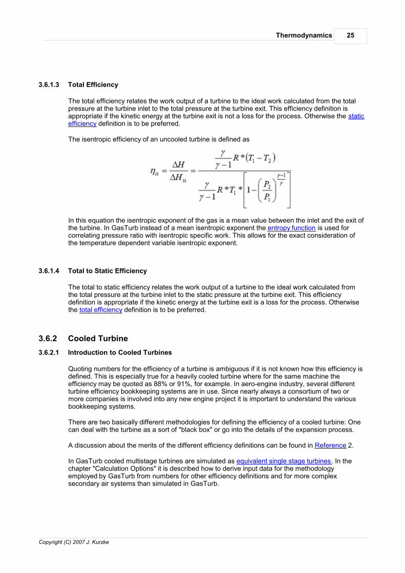
The isentropic efficiency of an uncooled turbine is defined as

In this equation the isentropic exponent of the gas is a mean value between the inlet and the exit ofthe turbine. In GasTurb instead of a mean isentropic exponent the entropy function is used forcorrelating pressure ratio with isentropic specific work. This allows for the exact consideration ofthe temperature dependent variable isentropic exponent.

3.6.1.4 Total to Static Efficiency

The total to static efficiency relates the work output of a turbine to the ideal work calculated fromthe total pressure at the turbine inlet to the static pressure at the turbine exit. This efficiencydefinition is appropriate if the kinetic energy at the turbine exit is a loss for the process. Otherwisethe total efficiency definition is to be preferred.

3.6.2 Cooled Turbine

3.6.2.1 Introduction to Cooled Turbines

Quoting numbers for the efficiency of a turbine is ambiguous if it is not known how this efficiency isdefined. This is especially true for a heavily cooled turbine where for the same machine theefficiency may be quoted as 88% or 91%, for example. In aero-engine industry, several differentturbine efficiency bookkeeping systems are in use. Since nearly always a consortium of two ormore companies is involved into any new engine project it is important to understand the variousbookkeeping systems.

There are two basically different methodologies for defining the efficiency of a cooled turbine: Onecan deal with the turbine as a sort of "black box" or go into the details of the expansion process.

A discussion about the merits of the different efficiency definitions can be found in Reference 2.

In GasTurb cooled multistage turbines are simulated as equivalent single stage turbines. In thechapter "Calculation Options" it is described how to derive input data for the methodologyemployed by GasTurb from numbers for other efficiency definitions and for more complexsecondary air systems than simulated in GasTurb.

26 GasTurb Details


3.6.2.2 Stage Efficiency of a Cooled Turbine

3.6.2.2.1 Single Stage Turbine

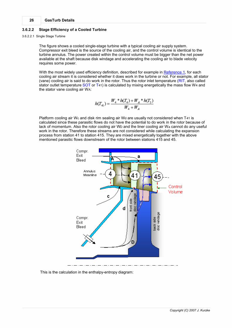
The figure shows a cooled single-stage turbine with a typical cooling air supply system.Compressor exit bleed is the source of the cooling air, and the control volume is identical to theturbine annulus. The power created within the control volume must be bigger than the net poweravailable at the shaft because disk windage and accelerating the cooling air to blade velocityrequires some power.

With the most widely used efficiency definition, described for example in Reference 1, for eachcooling air stream it is considered whether it does work in the turbine or not. For example, all stator(vane) cooling air is said to do work in the rotor. Thus the rotor inlet temperature (RIT, also calledstator outlet temperature SOT or T41) is calculated by mixing energetically the mass flow W4 andthe stator vane cooling air WA:

Platform cooling air Wc and disk rim sealing air Wd are usually not considered when T41 iscalculated since these parasitic flows do not have the potential to do work in the rotor because oflack of momentum. Also the rotor cooling air WD and the liner cooling air Wa cannot do any usefulwork in the rotor. Therefore these streams are not considered while calculating the expansionprocess from station 41 to station 415. They are mixed energetically together with the abovementioned parasitic flows downstream of the rotor between stations 415 and 45.

This is the calculation in the enthalpy-entropy diagram:

27Thermodynamics


With this approach the expansion process in the rotor is the same as in an uncooled turbine, andtherefore the number used for the efficiency can be understood as that for an uncooled turbine.

3.6.2.2.2 Two Stage Turbine

The figure shows the schematic of a two-stage cooled turbine with many secondary air streams.Such a turbine can be modeled with two different approaches. In the first approach the two-stageturbine is simulated as an equivalent single-stage turbine. Each secondary flow is assigned a workpotential. For example, the work potential of the first rotor cooling air will be approximately 50% asopposed to the 0% for a true single-stage turbine. Consequently the calculated rotor inlettemperature will no longer be equal to the true stator exit temperature T41 because more than justthe stator cooling air must be mixed with the main stream to get the equivalent rotor inlettemperature T41eq. This temperature is used to calculate the expansion process through theequivalent single-stage turbine.

28 GasTurb Details


The calculation - which is implemented in GasTurb - is basically the same as sketched in the h-sdiagram for a single stage turbine and yields for given total turbine power and pressure ratio theequivalent stage efficiency of the turbine.

The second approach to model the two-stage cooled turbine - which is not supported by GasTurb -follows the path shown in the h-s diagram below.

Each stage is modeled separately and the secondary airflows are mixed with the main stream atthe appropriate stations. The cooling air of the first vane is mixed upstream of the first rotor, andthe rest of the first stage secondary flows are mixed immediately downstream of the first rotor(station 42 in the first figure). Next the cooling air of the second vane is mixed, which yields theinlet mass flow W421 for the second rotor. At the exit of the second rotor the rest of the secondaryairflows are mixed with the mainstream.

With this approach one can study the effects of cooling air in a more direct way than with theequivalent single-stage approach. This, however, comes at a price: one needs to know theefficiency of each individual stage as well as the work distribution between the two rotors. Duringoff-design simulations one needs two turbine maps, one for each stage. These maps cannot bederived from engine tests because the required instrumentation is not available. Maps from a rigtest are not fully representative because in such a test the cooling air effects on the flow are nearlynever properly simulated because the temperature ratios between the cooling air and the mainstream are not as in the engine. Moreover, the map of the second stage is affected by the variableexit swirl of the first stage and therefore theoretically several maps for selected inlet swirl anglesare required.

3.6.2.3 Thermodynamic Turbine Efficiency

3.6.2.3.1 Definition of the Thermodynamic Turbine Efficiency

The second most used efficiency definition for a cooled turbine is called in literature the thermodynamic efficiency. In this approach the turbine is dealt with as a black box which convertsthermal energy into shaft power. The input into this black box are the main stream energy flow W4

*h(T4) and many secondary air streams Wi *h(Ti). All of these energy streams have the workpotential which results from an isentropic expansion from their individual total pressure Pi to theturbine exit pressure P45.

29Thermodynamics


The thermodynamic efficiency is defined as

The cooled turbine process is shown in the enthalpy-entropy diagram below. Note that within thisdefinition no stator outlet temperature needs to be calculated. PWpump is the shaft power requiredto accelerate the rotor cooling air to blade velocity.

The advantage of this turbine efficiency definition is that no assumptions have to be made aboutthe work potential of the individual secondary streams. The work potential of these streams isdefined via their respective pressures and temperatures, which at least theoretically all can bemeasured. Thus the use of the thermodynamic turbine efficiency is less ambiguous than all theother methods mentioned above. Moreover, the thermodynamic turbine efficiency accounts for thepressure of the secondary streams while all the other definitions do not.

The thermodynamic turbine efficiency is calculated within GasTurb and offered as an outputproperty for analysis or for being used as iteration target.

3.6.2.4 Calculation Options

3.6.2.4.1 Turbine Stage Number and Tabular Data Input

When you come first time to the cooled turbine main window you must load one of the data sets:

There are data sets for single stage turbines, two-stage turbines and three stage turbines. If youwork with a turbine which has more than three stages then use the three-stage turbine example.When you use GasTurb Details 5 for the first time then open one of the demo data sets, for atwo-stage turbine load the file Demo2Stg.TEF, for example.

30 GasTurb Details


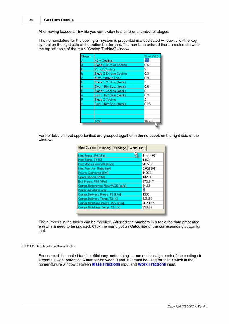
After having loaded a TEF file you can switch to a different number of stages.

The nomenclature for the cooling air system is presented in a dedicated window, click the keysymbol on the right side of the button bar for that. The numbers entered there are also shown inthe top left table of the main "Cooled Turbine" window.

Further tabular input opportunities are grouped together in the notebook on the right side of thewindow:

The numbers in the tables can be modified. After editing numbers in a table the data presentedelsewhere need to be updated. Click the menu option Calculate or the corresponding button forthat.

3.6.2.4.2 Data Input in a Cross Section

For some of the cooled turbine efficiency methodologies one must assign each of the cooling airstreams a work potential. A number between 0 and 100 must be used for that. Switch in thenomenclature window between Mass Fractions input and Work Fractions input.

31Thermodynamics


Note that the work fractions can only be modified in the nomenclature window.

3.6.2.4.3 Efficiency Definition Options

Four different options for defining the efficiency of a cooled turbine are implemented. Click one ofthe four leftmost tabs of the notebook at the bottom of the "Cooled Turbine" window and you getbesides the numbers also a graph with the corresponding definition of efficiency. Click the graph toenlarge it for better visibility.

3.6.2.4.4 Correlations Between Efficiencies

The number for the efficiency of a cooled turbine depends on the simulation methodologyemployed. In the lower part of the "Cooled Turbine" window you find the numbers for each of theefficiency definitions. Especially you find for each of the definitions a table with the numbers to beused with GasTurb which employs the equivalent single stage efficiency definition.

32 GasTurb Details


3.7 Mixing

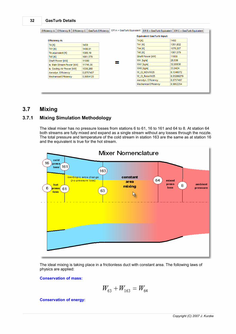
3.7.1 Mixing Simulation Methodology

The ideal mixer has no pressure losses from stations 6 to 61, 16 to 161 and 64 to 8. At station 64both streams are fully mixed and expand as a single stream without any losses through the nozzle.The total pressure and temperature of the cold stream in station 163 are the same as at station 16and the equivalent is true for the hot stream.

The ideal mixing is taking place in a frictionless duct with constant area. The following laws ofphysics are applied:

Conservation of mass:

Conservation of energy:

33Thermodynamics


Conservation of momentum:

Furthermore the sum of the cold and hot mixing areas is equal to the total area and the staticpressures of both streams are equal:

This system of equations can only be solved by iteration.

The flow is expanded from the conditions at station 8 through the nozzle to ambient pressure andwe get the gross thrust for the fully mixed flow. The gross thrust which could be developed byexpanding the hot flow from station 6 through the same type of nozzle is called the hot thrust Fg,h.Similarly the cold stream expanded from station 16 yields the cold thrust Fg,c. The unmixed thrustis the sum of Fg,h and Fg,c.

Mixing efficiency is defined as:

3.7.2 Mixer Input Data

Note that you can either specify the Mach number or the area, but not both:

Hot Mach No. Station 61 or Hot Area Station 61Cold Mach No. Station 161 or Cold Area Station 161Mixed Mach Number or Mixer Area (Station 64)

34 GasTurb Details


3.8 Nozzle

3.8.1 Convergent Nozzle

The basic setup of the calculation in GasTurb Details 5 is for a convergent-divergent nozzle.

For a convergent nozzle the exit area ratio A9/A8 must be set to 1.0. The calculation is fairlysimple: first an isentropic expansion to ambient pressure is calculated. If the resultant Machnumber is subsonic, then the static conditions in the nozzle exit plane have already been found.Otherwise the nozzle exit Mach number is set to 1.0 and from this condition new values for Ts,8

and Ps,8 are calculated.

3.8.2 Convergent Divergent Nozzle

For the convergent-divergent nozzle the flow from station 8 to station 9 is expanded supersonicallyaccording to the prescribed area ratio A9/A8. If the nozzle exit static pressure Ps,9 is higher thanambient pressure then the solution has been found and the calculation is finished. Otherwise, avertical shock is calculated. The position of the shock inside respectively outside of the divergentpart of the nozzle is found from conservation of mass, momentum and energy.

In the graph you can interactively modify the nozzle area ratio A9/A8 and the nozzle pressure ratioP8/Pamb. Start with a high pressure ratio and then increase the nozzle back pressure Pamb. Whenthe back pressure exceeds a certain value - which depends on the nozzle area ratio - you will seea vertical shock moving into the divergent part of the nozzle. If the nozzle pressure ratio is very lowthen the flow will be entirely subsonic.

The input data for a nozzle calculation are

35Thermodynamics


3.8.3 Ideal Thrust Coefficient

The ideal thrust coefficient relates the gross thrust of a nozzle to the thrust which could beachieved by expanding the flow ideally to ambient pressure. It is equal to 1.0 if the exit area ratio A9/A8 of a convergent-divergent nozzle is such that in the nozzle exit plane A9 the static pressure isequal to the ambient pressure.

4 Disk Design

4.1 Introduction

In GasTurb, if you select More in the program opening window, then you can calculate for manyengine configurations the basic geometry of the gas turbine including disk geometry and diskstress. The shape of the disk can be adapted in such a way that the Design Margin is equal to aspecified value, expressed in percent. You can deal with each of the disks separately employing GasTurb Details 5 and feed back the results into the cycle program.

A computer code for gas turbine engine weight and disk life estimation is described in Ref. 6; Manyof the ideas found there have been used for setting up the disk design algorithms, the help systemand the manual of this program. It must be acknowledged that the disk stress calculationmethodology employed has its limitations. In an actual disk, the local stresses - which are relevantfor disk live - depend on countless details which are not yet known in the preliminary design phaseof an engine.

Before any disk calculation can be performed, a disk design data set must be read from file. Thiscan be from a file with input data for a single disk, created with GasTurb Details 5, or from a GasTurb file which can contain the design data of many disks.

From GasTurb Details 5, when you are done with the design of a disk, you can write the optimizedgeometry either to a new file or you can update the data in the appropriate GasTurb file.

4.2 Disk Geometry

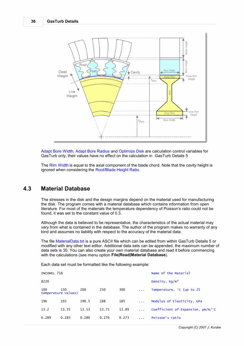
Disks are divided into two parts: the live disk and the part where the blades are attached. The diskstress calculation deals only with the live disk which carries the rim load caused by the blades(including shroud, inner platform and root) and the posts holding the blades. With other words, anymaterial outside of the smallest radius of the cavities (see figure) is dead weight which producesthe disk rim load.

36 GasTurb Details


Adapt Bore Width, Adapt Bore Radius and Optimize Disk are calculation control variables for GasTurb only, their values have no effect on the calculation in GasTurb Details 5

The Rim Width is equal to the axial component of the blade chord. Note that the cavity height isignored when considering the Root/Blade Height Ratio.

4.3 Material Database

The stresses in the disk and the design margins depend on the material used for manufacturingthe disk. The program comes with a material database which contains information from openliterature. For most of the materials the temperature dependency of Poisson's ratio could not befound, it was set to the constant value of 0.3.

Although the data is believed to be representative, the characteristics of the actual material mayvary from what is contained in the database. The author of the program makes no warranty of anykind and assumes no liability with respect to the accuracy of the material data.

The file MaterialData.txt is a pure ASCII file which can be edited from within GasTurb Details 5 ormodified with any other text editor. Additional data sets can be appended, the maximum number ofdata sets is 30. You can also create your own material database and read it before commencingwith the calculations (see menu option File|Read|Material Database).

Each data set must be formatted like the following example:

INCONEL 718 Name of the Material

8220 Density, kg/m³

100 150 200 250 300 ... Temperature, °C (up to 25temperature values)

196 193 190.5 188 185 ... Modulus of Elasticity, GPa

13.2 13.35 13.53 13.71 13.89 ... Coefficient of Expansion, µm/m/°C

0.289 0.283 0.280 0.276 0.273 ... Poisson's ratio

37Disk Design


1170 1150 1130 1110 1090 ... Yield Strength, MPa

1385 1375 1360 1352 1345 ... Ultimate Strength, MPa

| | | | |

1 11 21 31 41 ... Column

Note that the blue text is for explanation of the file structure only, do not include it in your materialdatabase file. Sorry for people who normally do not use SI units: this database must not containdata in US units, only the SI units indicated in the blue explanations are allowed.

If you find graphics with material data in literature, you can scan it and read the data from thebitmap with GasTurb Details 5!

4.3.1 INCONEL 601

INCONEL® 601 is a general purpose nickel-chromium-iron alloy for applications that requireresistance to heat and corrosion. In gas turbines it is used for combustion-can liners, diffuserassembles and containment rings.

Source of Data:www.specialmetals.com

4.3.2 INCONEL 706

INCONEL 706 nickel-iron-chromium alloy provides high mechanical strength in combination withgood fabricability. In the aerospace field, the alloy is used for compressor and turbine disks, shaftsand cases. In large industrial gas turbines it is used for turbine disks.

The heat treatments used are designed to produce either high stress-rupture properties (INCONEL706A) for applications up to 705°C (1300°F) or high tensile properties for moderate-temperatureapplications (INCONEL 706B).

Source of Data:www.specialmetals.comwww.hightempmetals.com

4.3.3 INCONEL 718

INCONEL 718 is a high strength, corrosion-resistant nickel chromium material used up to 700°C(1300°F) for rings and casings.


4.3.4 UDIMET R41

Common trade names: Rene 41®, Allvac Rene® 41, Haynes® R-41, Udimet® R41

UDIMET® R41 is a nickel-chromium alloy with extremely high room and elevated temperaturemechanical properties. It is used in critical aircraft engine components such as nozzle partitions,turbine blades and disks, combustion chamber liners and structural hardware.

Source of Data:www.specialmetals.comwww.hightempmetals.comwww.magellanmetals.com/Rene41.htm

http://www.specialmetals.com


http://www.hightempmetals.com/




http://www.magellanmetals.com/Rene41.htm

38 GasTurb Details


4.3.5 UDIMET 720

UDIMET alloy 720 is a nickel base alloy which combines high strength with metallurgical stability.Good oxidation and corrosion resistance combined with high strength make it useful in gas turbineblade and disk applications.

Note:

Unfortunately the temperature dependence of the modulus of elasticity and the thermal expansioncoefficient are not contained in the reference. These dependencies have been estimated, and thisestimate is certainly inaccurate.


4.3.6 Waspaloy

Waspaloy is a nickel-base superalloy with excellent high-temperature strength and good corrosionresistance at service temperatures up to 650°C (1200°F) for critical rotating applications and up to870°C (1600°F) for less demanding applications.

Source of Data:www.specialmetals.comhttp://asm.matweb.com/search/specificMaterial.asp?bassnum=NHWASA

4.3.7 Haynes 282

Haynes alloy 282 is a superalloy for potential applications in aircraft and land based gas turbines.At high temperatures, even as high as 900°C (1650°F) this alloy is stronger than Hynes Waspaloyand approaches the strength of Haynes R-41 alloy. It has much improved thermal stability,weldability and fabricability compared to Waspaloy and R-41 alloys.

Source:www.haynesintl.com

4.3.8 Greek Ascoloy (418)

Greek Ascoloy (418) is a stainless steel designed for services at temperatures up to 650°C (1200°F). Typical applications in gas turbines are compressor parts.

Source of Data:www.hightempmetals.com

4.3.9 AM 350

Alloy AM 350 is a chromium-nickel-molybdenum stainless steel which has been used forcompressor components such as blades, disks and shafts.


4.3.10 N-155 (Multimet)

N-155 Multimet is recommended for applications involving high stresses at temperatures up to815°C (1500°F) and can be used up to 1100°C (2000°F) where only moderate stresses areinvolved. It is used in gas turbines for exhaust manifolds, combustion chambers and turbineblades.



http://asm.matweb.com/search/specificMaterial.asp?bassnum=NHWASA

http://www.haynesintl.com



39Disk Design



4.3.11 Alloy A-286

The A-286 Iron-Nickel-Chromium alloy is designed for applications requiring high strength andgood corrosion resistance at temperatures up to 70°C (1300°F). It has been used in jet engines forturbine wheels and blades, casings and afterburner parts.

Source of Data:www.specialmetals.comwww.hightempmetals.com

4.3.12 Haynes 188

Haynes 188 is a superalloy with excellent high temperature strength and excellent resistance tooxidizing environments up to 1100°C (2000°F). It is widely used for fabricated parts in gas turbineengines.

Source of Data:www.specialmetals.comwww.haynesintl.com

4.3.13 Ti-6Al-4V

This alloy is the workhorse alloy of the titanium industry; It is used up to approximately 400°C (750°F) for blades, discs and rings.

Source of Data:

http://www.stainless-steel-world.net/titanium/alloys.aspwww.efunda.com/materials/alloys/titaniumvarious publications

4.4 Stress Calculation

4.4.1 Rim Load

The rim load is calculated considering the individual masses of the blades (including the shroud),the blade roots (including the blade platforms) and those parts of the disk that are located betweenthe blade roots, dubbed the posts. For each of these elements the product of mass, center ofgravity and rotational speed yield a contribution to the radial forces pulling at the rim of the livedisk. The rim stress sr,rim is the sum of all the forces divided by the live disk rim area.

Besides the flow annulus dimensions and the number of blades nb only a few more quantities areneeded for the rim load estimation. The Root/Blade Height Ratio is usually much higher with highpressure turbines compared to low pressure turbines. Note that with Mean Blade Thickness, [%] ofChord the thickness of the metal is meant which is in case of cooled or hollow blades less than themean profile thickness. Furthermore, one should not mix up the profile thickness quoted by theaerodynamicists with the mean blade thickness employed here.

The rim load estimation employs some empirical correlations which can not be representative forevery case. However, by using adequate input values for the Mean Blade Thickness and the Root/Blade Height Ratio a realistic value for the rim load can be achieved.





http://www.haynesintl.com

http://www.stainless-steel-world.net/titanium/alloys.asp

http://www.efunda.com/materials/alloys/titanium

40 GasTurb Details


4.4.1.1 Airfoil Mass

At first the true mean blade chord cb,mean is calculated from the axial chord (which is equal to the

the rim width trim ) assuming 35° stagger angle (cos 35°=0.82):

Blade taper must be taken into account by using an adequate value for the mean thickness/chordratio (t/c)b,mean when calculating the mean blade material thickness tb:

The mass of a single airfoil maf (made of a material with the density rb) is

Its center of gravity is more inbound than the mean annulus radius because of blade taper:

Blade shrouds, if they exist, are assumed to have a mean thickness which is approximately 5% ofthe rim width. Thus the mass of a single shroud is:

The center of gravity of the shroud is at the radius

This formula takes into account that the shroud is not only a simple plate, on top of it there areso-called tip fences which shift the center of gravity of the shroud to a higher radius than themean radius of the shroud plate.

4.4.1.2 Blade Attachment

The blade attachment is comprised of the blade platform, the neck and the fir tree. The neck existsonly if the total height of the blade root is bigger than the sum of blade platform thickness and thefir tree height.

41Disk Design


The total height of the blade root hroot = rroot- rrim is calculated from the given values for blade height

and root/blade height ratio. The blade platform thickness tplatform is set to 5% of the rim width. The

fir tree height hfir tree= rneck,i- rrim is assumed to be not greater than the blade platform width hfir tree,

max= 2*p*rroot/nb. The inner radius of the neck becomes rneck,i = rrim + hfir tree,max. If rneck,i happens to

be greater than rroot- tplatform then no neck exists, rneck,i is set to rroot- tplatform and the fir tree height is

reduced to rroot- tplatform- rrim.

Mass of the blade platform is

and the fir tree mass is

The posts extend to the radius rpost,o which is set to rrim+ 0.8*(rneck,i - rrim). Their mass is (disk

material density rd) :

If the neck exists, then its thickness is assumed to be twice as that of the blade:

The center of gravity for these elements is assumed to be at their respective mean radius. Thetotal dead mass per blade is

42 GasTurb Details


The center of gravity of the dead weight is at the radius:

Finally, the total rim load is

4.4.1.3 Blade Examples

4.4.1.3.1 High Pressure Turbine Blade

Unshrouded high pressure turbine blade

43Disk Design


4.4.1.3.2 Low Pressure Turbine Blade

Shrouded low pressure turbine blade with two tip fences

4.4.1.3.3 Turbine Blade with Root Neck

Shrouded turbine blade with root neck

4.4.2 Disk Stress Analysis

The disk stress analysis is based on the following differential equations (see Ref. 6):

Equilibrium of forces for a disk element:

Radial stress:

44 GasTurb Details


Tangential Stress:

E N/m² modulus of elasticity

r m radius

t m disk thickness

u m radial displacement

a 1/°C coefficient of thermal expansion

g - Poisson’s ratio

srN/m² radial stress

stN/m² tangential stress

w rad/s rotational speed

DT °C temperature above reference (room) temperature

For the stress calculation in GasTurb Details 5 the differential equations above are converted intofinite difference equations which are applied to many rings in which the live disk is divided. In thedisk bore (the inner area of the innermost ring) the radial stress sr is zero. When the calculation

begins, the displacement of the bore is estimated and the differential equations yield the radial andthe tangential stresses as well as the displacement at the outer radius of the first ring. Thesequantities allow then to calculate the conditions of the second and the further rings. Finally all therings have been calculated and the radial stress at the outer radius of the live disk is found. Aslong as this radial stress is not equal to the rim load, the estimated bore displacement is iterativelycorrected until the rim load is equal to the calculated radial stress at the outer radius of the livedisk.

The temperature distribution in the disk is assumed to vary linearly between the bore and the rimtemperatures. The reference temperature is 20°C; for this temperature no stress exists in a non-rotating disk.

4.4.3 Design Criteria

The disk stress calculation should be done for the maximum steady state rotational speed and thehighest operating temperatures. If the operating point with the highest temperature does notcoincide with the operating point which has the highest rotational speed then both conditionsshould be checked.

The disk design margin (expressed in %) compares the yield strength of the material at the localtemperature s0.2,local with the local von Mises stress svon Mises:

45Disk Design


The lowest local design margin is presented as output quantity. Moreover, the stress margins atthe bore and at the web outer diameter, just below the disk rim, are available as design criteria.

No safety margins are considered, it is up to you to design the disk for the positive stress marginyou consider appropriate (10...30% are reasonable numbers).

The disk burst margin (in %) compares the ultimate strength of the material sultimate (evaluated at

the average disk temperature) with the average tangential stress:

The factor 0.47 (taken from Ref. 6) is a sort of safety margin and therefore Burst Margin ³ 0 is areasonable design target.

The disk burst speed - which should be greater than 130...150% of the operating speed - iscalculated as

For the optimization of the disk geometry its mass and the polar moment of inertia of the bladeddisk are important properties.

4.5 Optimization

A numerical optimization routine is build into GasTurb Details 5 which allows to optimize thegeometry of disks. First select your optimization variables and set lower and upper boundaries forthese variables. Next choose the constraints that are relevant for your problem and finally select aquantity as figure of merit which is to be maximized or minimized. Note that the starting point of theoptimization must be within the permissible range boundaries of the variables and the constraints.

Two optimization strategies are offered: a gradient strategy and the adaptive random searchstrategy. On a modern computer the time needed for an optimization is so short that the speeddifferences between the two strategies is of no relevance. If you are in doubt whether the trueoptimum has been found, try both strategies. Note that the random search algorithm uses for eachrun a new set of random numbers and therefore the optimization result will be slightly different foreach time you run this algorithm.

The range between the minimum and the maximum values for the optimization variables has aninfluence on the precision of the result: A small range yields high accuracy, however, there is thedanger that unintentionally the true optimum is excluded by too narrow range boundaries.

Example:

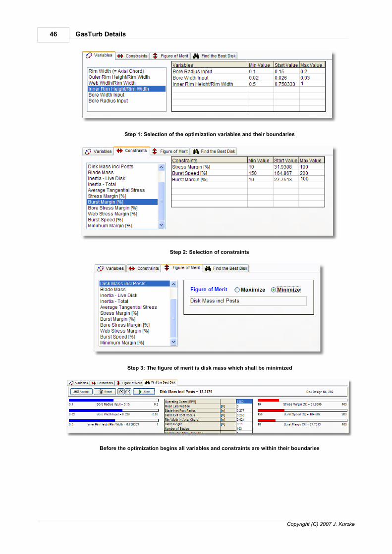
46 GasTurb Details


Step 1: Selection of the optimization variables and their boundaries

Step 2: Selection of constraints

Step 3: The figure of merit is disk mass which shall be minimized

Before the optimization begins all variables and constraints are within their boundaries

47Disk Design


After the optimization one variable and two of the three constraints are at their respective boundaries.

Disk weight is reduced from 13.2175 to 11.0325 kg in this example

4.6 Terminology

Tensile Strength

Tensile strength measures the force per cross sectional area required to pull a test specimento the point where it breaks. While the stress is low, the length of the material will increaseproportional to the force applied. When the force is removed, then the material will relax to itsoriginal shape. When a certain stress is exceeded, then a plastic deformation happens and theshape of the material will change permanently.

Yield Strength

The stress a material can withstand without permanent deformation

Ultimate Stress

The maximum stress a material can withstand

48 GasTurb Details


von Mises Stress

von Mises stress is a combination of stresses in two or three dimensions which can becompared to the tensile strength of a material loaded in one dimension

Poisson's ratio

During a tensile test, the reduction in cross-sectional area is proportional to the increase inlength in the elastic range. The ratio of transverse contraction to longitudinal extension of thematerial is Poisson's ratio.

5 Digitizing a Picture

5.1 The Task

You may have information in form of a picture, but you need numbers. For example, you may havegot a gas turbine manufacturers brochure with performance data and you want to model theperformance of this engine with GasTurb.

When you have these data numerically, then you can use them as Comparative Data that areshown in the GasTurb graphical output together with the simulation results. Another applicationexample for this program option would be if you have measured data only as a picture and notnumerically.

With GasTurb Details 5 you can read any graphic in bitmap format, show it on your computerscreen and pick the numbers from the picture with mouse button clicks.

49Digitizing a Picture


5.2 Setting the Scales

After having selected Read from a Graphic in the program opening window the first action isreading a graphic in bitmap format (file extension bmp). Next the scales of the graphics must becorrelated with the pixel coordinates on the screen.

A blinking square and two blinking triangles appear in the top left corner of the graphic. With thesesymbols you must mark the axes: the square is for the origin where the y-axis crosses the x-axis.First click the point in the center of the blinking square, keep the mouse button pressed and moveit to the origin of the graphic. After releasing the button, the true numbers of the graphics originmust be input in the two edit fields which appear. In the example below the true x value of theorigin is -45 and the true y value is 30. Click the OK Button to proceed with one of the two blinkingtriangles. Place the triangle pointing to the right to the end of the x-axis and the triangle pointingupwards to the upper end of the y-axis.

When you set the upwards pointing triangle, then the true x-value is shown in a disabled edit field;you can only input the true y value for the marked point. Similarly, when you set the true x value forthe right end of the x axis, the true y value is shown in a disabled field.

50 GasTurb Details


After having set the origin as well as the end values for the x and y axis you can go for pickingnumbers from this graph.

5.3 Reading Numbers

Before commencing with picking numbers you should edit the table column headings. After thatclick the menu option Pick|Read Numbers or click the second button from the right. While youmove the mouse pointer over the image you will see the numbers which will be transferred to thetable when you click on the graphic. If you accidentally click a wrong spot then erase it by clickingthe rightmost button.

Each click fills a line in the table and produces a cross in the graphic:

51Digitizing a Picture


Often you will have only one line in your graphic. When you are done with picking numbers fromthis single line then you must save them to a text file before closing the window. However, as in theexample above there might be several quantities plotted over the same x-axis. How to handle sucha situation is described in the following section.

5.4 Several Lines

After having finished the number picking for the first line you can go for a second and a third linewhich have a common x-axis with the first line. To initiate a new line select the menu option Pick|New Property or click the corresponding button. You will get the opportunity to enter a headline forthe next column in the table before the number picking begins.

The new property may be assigned to the same y-axis or to a different y-axis. In the latter case youmust reset the y-scale which can be done after clicking the button marked with a little key. Clickthe point in the triangle at the y-axis (without moving the mouse) and enter the new true y value forthe end of this axis and similarly adapt the true y value of the origin value after clicking the point in

52 GasTurb Details


the blue square. When the new scaling is completely defined, then you can pick numbers again.Note that you can not modify or add new x-values at this stage of the work.

6 References

[1] P. P. Walsh, P. FletcherGas Turbine PerformanceBlackwell Science Ltd,1998

[2] J. KurzkePerformance modeling methodology: Efficiency definitions for cooled single andmultistage turbinesASME paper 2002-GT-30497 presented at the Turbo Expo 2002 in Amsterdam

[3] Arthur J. GlassmanUsers Manual for Updated Computer Code for Axial Flow Compressor Conceptional DesignNASA Contractor Report 189171, 1992

[4] Arthur J. GlassmanComputer Program for Preliminary Design Analysis of Axial Flow TurbinesNASA TN D-6702, 1972

[5] Sanford GordonThermodynamic and Transport Combustion Properties of Hydrocarbons With AirNASA TP 1906, 1982

[6] Michael T.Tong, Ian Halliwell, Louis J. GhosnA Computer Code for Gas Turbine Engine Weight and Disk Life EstimationJournal of Engineering for Gas Turbines and Power, April 2004, V0l. 126, pp 265-270

Index 53


Index

- A -A286 39

Airfoil Mass 40

Airspeed 18

AM 350 38

Area Ratio 16Nozzle 34

Assigned Enthalpy 12

Atom Ratio 12

Axial Flow Compressor 20

Axial Turbine Turbine Design 24

- B -Bitmap 48

Blade HP Turbine 42, 43

LP Turbine 43

Blade Exit Root Radius 35

Blade Inlet Root Radius 35

Blade Mass 40

Bore Radius 35

Bore Width 35

Burner 20

Burst Speed 44

- C -C/D Nozzle 34

Calibrated Airspeed 18

CEA 11, 12

Chemical Equilibrium 13

Combustion 20

Comparative Data 48

Compression Calculation 19

Convergent-Divergent Nozzle 34Ideal Thrust Coefficient 35

Cooled Turbine Efficiency Correlations 31

Efficiency Options 31

GasTurb Efficiency Definition 31

Introduction 25

Mass and Work Fractions 30

Nomenclature 30

Single Stage 26

Stage Number 29

Thermodynamic Efficiency 28

Two Stages 27

Cooling Air Work Potential 26, 27

Corrected Flow per Area 16

Corrected Power Offtake 18

- D -Deleting a Fuel 14

Design Margin 44

Diesel 11

Digitizing a Picture 48

Disk Design Criteria 44

Geometry 35

Hyperbolic 35

Live Disk 35

Material Database 36

Optimization 45

Posts 39

Rim Load 39

Ring 35

Stress Analysis 43

Web 35

Dissociation 13, 20

Duct 22

- E -Efficiency

Cooled Turbine 25, 31

Single Stage Cooled Turbine 26

Thermodynamic (Cooled Turbine) 28

Two Stage Cooled Turbine 27

Enthalpy 14

Entropy Function 15

Equilibrium Temperature 13

Equivalent Stage Efficiency 27

Equivalent Turbine Efficiency 31

Equivalent Turbine Inlet Temperature 31

Equivaluent Airspeed 18

Exit Corrected Flow 20

Expansion Calculation 23

- F -Fanno-Line 22

FCEA2 11, 12First Run 13

Second Run 14

Flight Conditions 18

Friction Pressure Loss 22

Fuel 11

GasTurb Details54


Fuel 11Delete 14

Name 12

New 11, 14

Temperature 13

Fuel-Air-Ratio Range 13

Fundamental Pressure Loss 22

- G -Gas Properties

Dissociation 13

Enthalpy 14

Entropy Function 15

Gas Constant 10

Isentropic Exponent 15

Numbers 16

Gas Property Data Files 12

GasTurb Efficiency Definition for Cooled Turbines 31

GasTurb Equivalent Turbine Efficiency 31

Generic Fuel 11

Graphic 8

Greek Ascoloy 38

Grid 8

- H -Half-Ideal Gas 10

Haynes 188 39

Haynes 282 38

Heat Addition 20

Heat Exchanger 21

Heat of Formation 12

Help Installation on a Network 7

Hyperbolic Disk 35

- I -Ideal Gas 10

Ideal Thrust Coefficient 35

INCONEL 601 37

INCONEL 706 37

INCONEL 718 37

Indicated Airspeed 18

Installation 7

Introduction 7

Isentropic 15

Isentropic Exponent 15

Isentropic Flow 16, 17

- J -JP-10 11

JP-4 11

- L -Live Disk 35

Loss Correction Factor 20

- M -Make Gas Property File 14

Mass Fraction 12

Material Blades, Disks and Structural Components 37

Combustion Can Liners, Containment Rings 37

Combustors, Flameholders 39

Compressor Blades, Disks and Rings 39

Compressor Disks and Blades 38

Critical Rotating Applications 38

Disks, Shafts and Casing 37

Rings and Casings 37

Turbine Blades, Combustors 38

Turbine Blades, Disks 38

Turbine Disks and Blades 39

Material Database 36A286 39

AM 350 38

Greek Ascoloy 38

Hanes 282 38

Haynes 188 39

Haynes R41 37

INCONEL 601 37

INCONEL 706 37

INCONEL 718 37

Multimet 38

N-155 38

Rene 41 37

Ti-6Al-4V 39

UDIMET 720 38

UDIMET R41 37

Waspaloy 38

Mixer Input Data 33

Methodology 32

Mole Fraction 12

- N -N-155 (Multimet) 38

NASA CEA code 11

NASA Efficiency Correlation

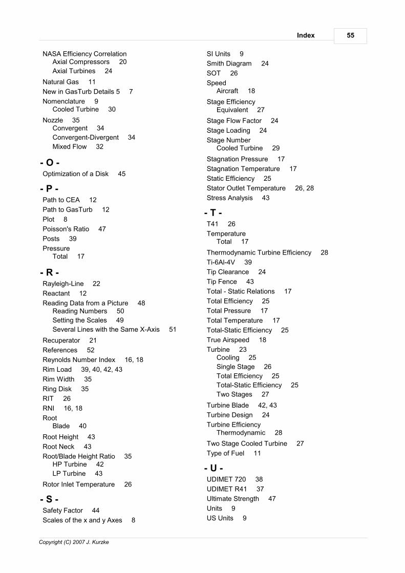
Index 55


NASA Efficiency Correlation Axial Compressors 20

Axial Turbines 24

Natural Gas 11

New in GasTurb Details 5 7

Nomenclature 9Cooled Turbine 30

Nozzle 35Convergent 34

Convergent-Divergent 34

Mixed Flow 32

- O -Optimization of a Disk 45

- P -Path to CEA 12

Path to GasTurb 12

Plot 8

Poisson's Ratio 47

Posts 39

Pressure Total 17

- R -Rayleigh-Line 22

Reactant 12

Reading Data from a Picture 48Reading Numbers 50

Setting the Scales 49

Several Lines with the Same X-Axis 51

Recuperator 21

References 52

Reynolds Number Index 16, 18

Rim Load 39, 40, 42, 43

Rim Width 35

Ring Disk 35

RIT 26

RNI 16, 18

Root Blade 40

Root Height 43

Root Neck 43

Root/Blade Height Ratio 35HP Turbine 42

LP Turbine 43

Rotor Inlet Temperature 26

- S -Safety Factor 44

Scales of the x and y Axes 8

SI Units 9

Smith Diagram 24

SOT 26

Speed Aircraft 18

Stage Efficiency Equivalent 27

Stage Flow Factor 24

Stage Loading 24

Stage Number Cooled Turbine 29

Stagnation Pressure 17

Stagnation Temperature 17

Static Efficiency 25

Stator Outlet Temperature 26, 28

Stress Analysis 43

- T -T41 26

Temperature Total 17

Thermodynamic Turbine Efficiency 28

Ti-6Al-4V 39

Tip Clearance 24

Tip Fence 43

Total - Static Relations 17

Total Efficiency 25

Total Pressure 17

Total Temperature 17

Total-Static Efficiency 25

True Airspeed 18

Turbine 23Cooling 25

Single Stage 26

Total Efficiency 25

Total-Static Efficiency 25

Two Stages 27

Turbine Blade 42, 43

Turbine Design 24

Turbine Efficiency Thermodynamic 28

Two Stage Cooled Turbine 27

Type of Fuel 11

- U -UDIMET 720 38

UDIMET R41 37

Ultimate Strength 47

Units 9

US Units 9

GasTurb Details56


- V -Velocity Diagram 24

von Mises Stress 44, 47

- W -Waspaloy 38

Web Disk 35

Web Width 35

What's New 7

Work Potential of Cooling Air 26, 27

- Y -Yield Stength 47

- Z -Zooming 8

Documents

GasTurb Details · The program GasTurb Details 5 is an utility which allows to do some basic calculations with the ... CH4 and 10% C2H6 is considered. Copyright (C)