Embed Size (px)
Citation preview
Gaussian Elimination and LU-Decomposition
Gary D. Knott
Civilized Software Inc.
12109 Heritage Park Circle
Silver Spring MD 20906
phone:301-962-3711
email:[email protected]
URL:www.civilized.com
January 9, 2014
1 Gaussian Elimination and LU-Decomposition
Solving a set of linear equations arises in many contexts in applied mathematics. At least untilrecently, a claim could be made that solving sets of linear equations (generally as a component ofdealing with larger problems like partial-differential-equation solving, or optimization, consumesmore computer time than any other computational procedure. (Distant competitors would be theGram-Schmidt process and the fast Fourier transform computation, and the Gram-Schmidt processis a first cousin to the Gaussian elimination computation since both may be used to solve systemsof linear equations, and they are both based on forming particular linear combinations of a givensequence of vectors.) Indeed, the invention of the electronic digital computer was largely motivatedby the desire to find a labor-saving means to solve systems of linear equations [Smi10].
Often the subject of linear algebra is approached by starting with the topic of solving sets of linearequations, and Gaussian elimination methodology is elaborated to introduce matrix inverses, rank,nullspaces, etc.
We have seen above that computing a preimage vector x ∈ Rn of a vector v ∈ Rk with respect tothe n× k matrix A consists of finding a solution (x1, . . . , xn) to the k linear equations:
A11x1 + A21x2 + · · ·+ An1xn = v1
A12x1 + A22x2 + · · ·+ An2xn = v2
...
A1kx1 + A2kx2 + · · ·+ Ankxn = vk.
This corresponds to xA = v.
1
1 GAUSSIAN ELIMINATION AND LU-DECOMPOSITION 2
If v ∈ Rk − rowspace(A) then there are no solutions x; the equations xA = v are inconsistent. Forexample, [1x1 + 2x2 = 0, 2x1 + 4x2 = 1]. This is because xA = x1(A row 1) + · · ·+ xn(A row n) ∈rowspace(A) ⊆ Rk for every x ∈ Rn.
Recall that nullspace(A) = {x ∈ Rn | xA = 0} with dim(nullspace(A)) = n − rank(A). Ifnullspace(A) = {0} and v ∈ rowspace(A), then the linear equations xA = v have the uniquesolution x = vA+, where the k × n matrix A+ is the Moore-Penrose pseudo-inverse matrix of A.Necessarily k ≥ n; in case n = k, A is non-singular and A+ = A−1 so x = vA−1. The vector vA+
always belongs to colspace(A) regardless of the choice of v or the dimension of nullspace(A).
More generally, if dim(nullspace(A)) ≥ 0 and v ∈ rowspace(A), there is a dim(nullspace(A))-dimensional flat of solutions x. The vectors in nullspace(A) + vA+ ⊆ Rn comprise all the solutionvectors, x, that satisfy xA = v. The matrix A corresponds to a mapping that maps the family ofparallel (n−rank(A))-dimensional flats {nullspace(A)+y | y ∈ colspace(A)} covering Rn to pointsin rowspace(A) ⊆ Rk; this flat-to-point mapping is one-to-one and onto.
Geometrically, with rank(A) = r and v ∈ rowspace(A), we have r linearly-independent hyperplanesdefined by (x, A col j1) = vj1 , . . ., (x, A col jr) = vjr where A col j1, . . . , A col jr are linearly-independent columns of A; these hyperplanes intersect in an (n − r)-dimensional flat in Rn; thisflat is the translation of nullspace(A): vA+ + nullspace(A).
In general, the matrix A+A is the k × k projection matrix onto rowspace(A) ⊆ Rk, and for anyvector v ∈ Rk, the vector vA+ is the unique vector in colspace(A) such that |v−vA+A| is minimal;moreover vA+ is a shortest minimizing vector in Rn.
We often wish to determine which of these cases (no solution, unique solution, multiple solutions)hold for a given n×k matrix A and a given righthand-side vector v ∈ Rk, and when v ∈ rowspace(A),we wish to compute a solution vector x = vA+ without the expense of computing the Moore-Penrosepseudo-inverse matrix A+. The classic step-wise approach to computing x is to add a multiple ofone equation to another at each step until the system of equations is reduced to a form which is easyto either solve or to see that no solution or no unique solution exists. This process is called Gaussianelimination, since we generally aim to eliminate successive variables from successive equations bysimple algebraic modifications as was proceduralized by C. F. Gauss [Grc11a].
The form that is most commonly sought is a triangular system of equations. We will usually onlyneed to deal with such a triangular system in the case where n = k and we have a unique solutionvector x, i.e., where we have a consistent system of equations with n = k, and the matrix ofcoefficients is non-singular. In this case, we can obtain:
L11x1 + L21x2 + · · · + Ln−1,1xn−1 + Ln1xn = y1
L22x2 + · · · + Ln−1,2xn−1 + Ln2xn = y2...
Ln−1,n−1xn−1 + Ln,n−1xn = yn−1
Lnnxn = yn
This corresponds to xL = y where L is an n× n lower-triangular matrix. Let us assume there is aunique solution, so L must be non-singular, and thus Lii is necessarily non-zero for i = 1, . . . , n. If
1 GAUSSIAN ELIMINATION AND LU-DECOMPOSITION 3
we have such a triangular form, then we have one equation involving just xn, one involving just xn
and xn−1, and so on, and it is easy to compute the solution vector x. The process of computing thesolution is called “back-substitution.” An algorithm for solving xL = y with back-substitution isgiven below. Note if we try to divide by zero, this algorithm will fail; this is why we require Lii 6= 0for 1 ≤ i ≤ n.
[for i = n, n− 1, . . . , 1 : (xi ← yi; for j = i + 1, . . . , n : (xi ← xi − Ljixj); xi ← xi/Lii)].
Exercise 1.1: State the back-substitution algorithm that applies when we have a non-singularn× n upper-triangular matrix U with xU = y, so that we have one equation involving just x1,one involving just x1 and x2, and so on.
Exercise 1.2: Write-out the matrix products xL and LTxT and compare them.
Exercise 1.3: Let A be a 1× k matrix. What is the lower-triangle of A?
Exercise 1.4: Let L be an n × n lower-triangular matrix. Why must Lii 6= 0 for 1 ≤ i ≤ nwhen L is non-singular?
Exercise 1.5: Show that the back-substitution algorithm given above uses n divisions, n(n−1)/2 multiplications and subtractions, and n(n + 3)/2 assignment operations to compute thevector x.
Exercise 1.6: When is the inverse of a non-singular n × n triangular matrix, L, itself trian-gular? Hint: consider determining the i-th row of L−1 by solving xL = ei.
Exercise 1.7: Show that if the i-th column of an n× n matrix L has Lji = 0 then (L col i)T
is normal to the natural basis vector ej . Thus when L is a lower-triangular matrix, (L col i)T
is normal to e1, e2, . . . , ei−1 for i = 2, . . . , n.
For the n × k matrix A with A 6= 0, we can approach solving the system of k equations with nunknowns xA = v as follows. For each variable xi with i = 1, 2, . . . , n, select an “eligible” equation(x, A col j) = vj with Aij 6= 0; this equation is called the pivot equation and the coefficient Aij
is called the pivot value for the elimination of xi. Solve this equation for xi, and then use thisexpression for xi to eliminate xi in all the other equations.
Specifically, given xi =∑
1≤h≤nh 6=i
−Ahj
Aijxh, we eliminate xi from the equation (x, A col p) = vp by
substituting∑
1≤h≤nh 6=i
−Ahj
Aijxh for xi in (x, A col p) = vp to obtain the equation
(x, [A col p]− Aip
Aij[A col j]) = vp −
Aip
Aijvj ,
in which the variable xi has been eliminated, (i.e., the coefficent of xi is zero.) Note this trans-formation replaces equation p with the sum of equation p and a multiple of equation j. (Thistransformation applied to all equations p with p 6= j is called a full-elimination or full-pivoting
1 GAUSSIAN ELIMINATION AND LU-DECOMPOSITION 4
iteration.) We then make equation j “ineligible” and proceed to try to eliminate the next variable,xi+1 from all but one of our equations (both eligible and ineligible,) continuing in this way untilthere are no eligible equations left or no variables appearing in multiple equations left to eliminate.Note if Aip = 0, xi is “already eliminated” in equation p and we need not proceed further toeliminate xi in equation p.
If we can succeed in eliminating each variable from all but one of our equations, and if each finalequation thus obtained contains no more than one variable, distinct from the variables in all theother equations, then we have “diagonalized” our system of equations; each equation is now eitherof the form “0 = v′j” or is of the form “A′
ijxi = v′j ,” with A′ij 6= 0. If we have any equation of the
form “0 = v′j” with v′j 6= 0, then our equations are inconsistent. Otherwise, we can easily obtainvalues of x1, . . . , xn that satisfy xA = v. (We have xi = v′j/A
′ij when A′
ij 6= 0, and we may take xi
to be an arbitrary value when A′ij = 0, i.e., when the “ equation for xi” is 0 = 0.)
Exercise 1.8: Is the qualifying clause “distinct from the variables in all the other equations”in the prior paragraph superfluous? Hint: yes.
This method of eliminating variables by forming linear combinations of the originally-given equa-tions, as well as variant methods which do not achieve a full “diagonalized” system of equations,are all called Gaussian elimination.
If we have more equations than unknowns (n < k,) then either these k equations are inconsistent,or at least k − n of these equations are linear combinations of the other equations. If exactly n ofthe k consistent equations are linearly-independent, there is a unique solution; otherwise we havefewer than n independent equations and we have an infinite number of solutions. If we have atleast as many unknowns as equations (n ≥ k,) then, unless these equations are inconsistent, there isalways at least one solution, and when n > k there are an infinite number of solutions. (There mayalso be an infinite number of solutions when n = k and there are fewer than n linearly-independentequations.)
Exercise 1.9: What do we mean by an “eligible” equation? Why do we make an equation“ineligible” after we use it to eliminate a variable from all the other equations? (Try usingthe same equation in two steps to eliminate two distinct variables x1 and x2 from all the otherequations in an example such as [x1 + x2 + x3 = 3, x1 − x2 − x3 = 1, x1 + x2 − x3 = 2].)
Alternately, we can try to “reduce” our system of equations xA = v to triangular form ratherthan diagonal form by “partially” eliminating each variable from our equations, i.e., variable xi
is eliminated from k − i equations when possible. This triangular form can be as useful as thediagonal form, and even more so when xA = v does not have a unique solution, and it can alsobe used to solve multiple systems of equations with distinct righthand-sides, with just two back-substitution steps for each such system. This is achieved by using Gaussian elimination as sketchedabove, but only eliminating the i-th variable xi from the k − i currently-“eligible” equations, notincluding the current pivot equation. This transformation is called tail-elimination. (What wemean by ‘triangular’ is that one equation contains only 1 variable, one equation contains at most2 variables, and so on. Note, in general, neither “true” diagonal or triangular forms of coefficientmatrix can be obtained unless we renumber, i.e., permute our variables and/or suitably order ourequations.)
1 GAUSSIAN ELIMINATION AND LU-DECOMPOSITION 5
It is important to note that, depending on the order of our equations and the numbering of ourvariables, constructing either a triangular or diagonal form may encounter very small pivot valuesand this may introduce excessive round-off error in the solution of the associated set of linearequations; we may use a “pivot search” for a large pivot value during each iteration to mitigate thisdanger. (Large pivot values are less problematic with respect to error.) The “partial” eliminationprocess to obtain a triangular form using round-off error-reduction measures is the subject to beaddressed below.
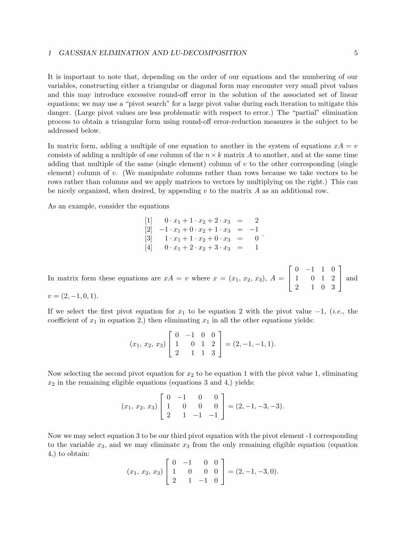
In matrix form, adding a multiple of one equation to another in the system of equations xA = vconsists of adding a multiple of one column of the n×k matrix A to another, and at the same timeadding that multiple of the same (single element) column of v to the other corresponding (singleelement) column of v. (We manipulate columns rather than rows because we take vectors to berows rather than columns and we apply matrices to vectors by multiplying on the right.) This canbe nicely organized, when desired, by appending v to the matrix A as an additional row.
As an example, consider the equations
[1] 0 · x1 + 1 · x2 + 2 · x3 = 2[2] −1 · x1 + 0 · x2 + 1 · x3 = −1[3] 1 · x1 + 1 · x2 + 0 · x3 = 0[4] 0 · x1 + 2 · x2 + 3 · x3 = 1
.
In matrix form these equations are xA = v where x = (x1, x2, x3), A =
0 −1 1 01 0 1 22 1 0 3
and
v = (2,−1, 0, 1).
If we select the first pivot equation for x1 to be equation 2 with the pivot value −1, (i.e., thecoefficient of x1 in equation 2,) then eliminating x1 in all the other equations yields:
(x1, x2, x3)
0 −1 0 01 0 1 22 1 1 3
= (2,−1,−1, 1).
Now selecting the second pivot equation for x2 to be equation 1 with the pivot value 1, eliminatingx2 in the remaining eligible equations (equations 3 and 4,) yields:
(x1, x2, x3)
0 −1 0 01 0 0 02 1 −1 −1
= (2,−1,−3,−3).
Now we may select equation 3 to be our third pivot equation with the pivot element -1 correspondingto the variable x3, and we may eliminate x3 from the only remaining eligible equation (equation4,) to obtain:
(x1, x2, x3)
0 −1 0 01 0 0 02 1 −1 0
= (2,−1,−3, 0).
1 GAUSSIAN ELIMINATION AND LU-DECOMPOSITION 6
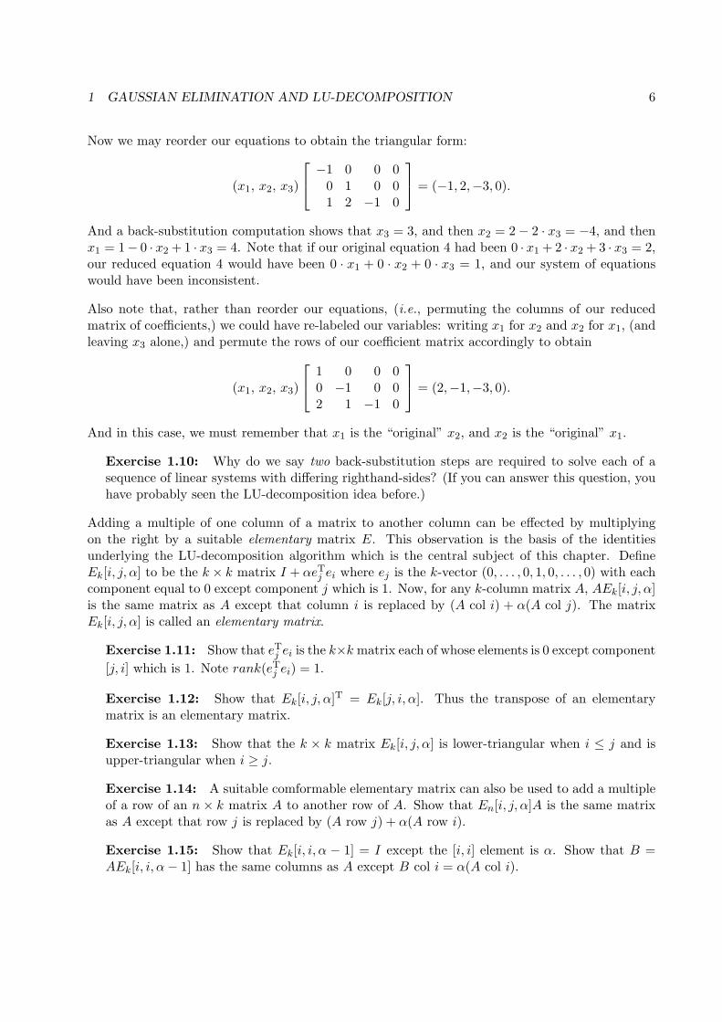
Now we may reorder our equations to obtain the triangular form:
(x1, x2, x3)
−1 0 0 00 1 0 01 2 −1 0
= (−1, 2,−3, 0).
And a back-substitution computation shows that x3 = 3, and then x2 = 2− 2 · x3 = −4, and thenx1 = 1− 0 · x2 + 1 · x3 = 4. Note that if our original equation 4 had been 0 · x1 + 2 · x2 + 3 · x3 = 2,our reduced equation 4 would have been 0 · x1 + 0 · x2 + 0 · x3 = 1, and our system of equationswould have been inconsistent.
Also note that, rather than reorder our equations, (i.e., permuting the columns of our reducedmatrix of coefficients,) we could have re-labeled our variables: writing x1 for x2 and x2 for x1, (andleaving x3 alone,) and permute the rows of our coefficient matrix accordingly to obtain
(x1, x2, x3)
1 0 0 00 −1 0 02 1 −1 0
= (2,−1,−3, 0).
And in this case, we must remember that x1 is the “original” x2, and x2 is the “original” x1.
Exercise 1.10: Why do we say two back-substitution steps are required to solve each of asequence of linear systems with differing righthand-sides? (If you can answer this question, youhave probably seen the LU-decomposition idea before.)
Adding a multiple of one column of a matrix to another column can be effected by multiplyingon the right by a suitable elementary matrix E. This observation is the basis of the identitiesunderlying the LU-decomposition algorithm which is the central subject of this chapter. DefineEk[i, j, α] to be the k × k matrix I + αeT
j ei where ej is the k-vector (0, . . . , 0, 1, 0, . . . , 0) with eachcomponent equal to 0 except component j which is 1. Now, for any k-column matrix A, AEk[i, j, α]is the same matrix as A except that column i is replaced by (A col i) + α(A col j). The matrixEk[i, j, α] is called an elementary matrix.
Exercise 1.11: Show that eTj ei is the k×k matrix each of whose elements is 0 except component
[j, i] which is 1. Note rank(eTj ei) = 1.
Exercise 1.12: Show that Ek[i, j, α]T = Ek[j, i, α]. Thus the transpose of an elementarymatrix is an elementary matrix.
Exercise 1.13: Show that the k × k matrix Ek[i, j, α] is lower-triangular when i ≤ j and isupper-triangular when i ≥ j.
Exercise 1.14: A suitable comformable elementary matrix can also be used to add a multipleof a row of an n × k matrix A to another row of A. Show that En[i, j, α]A is the same matrixas A except that row j is replaced by (A row j) + α(A row i).
Exercise 1.15: Show that Ek[i, i, α − 1] = I except the [i, i] element is α. Show that B =AEk[i, i, α− 1] has the same columns as A except B col i = α(A col i).
1 GAUSSIAN ELIMINATION AND LU-DECOMPOSITION 7
Exercise 1.16: Show that, if α = 0 or i 6= j then Ek[i, j, α]−1 = Ek[i, j,−α], if α 6= −1 andi = j then Ek[i, j, α]−1 = Ek[i, i,−α/(1+α)], and if α = −1 and i = j then Ek[i, j, α] is singular.
Exercise 1.17: Let the k × k matrix S = Ek[i, j,−1]Ek[j, i, 1]Ek[i, j,−1]Ek[i, i,−2], where1 ≤ i ≤ k and 1 ≤ j ≤ k with i 6= j. Show that B = AS has the same columns as A exceptB col i = A col j and B col j = A col i, where i 6= j. What does right-multiplication by S doif i = j?
Recall that transposek(i, j) denotes the permutation 〈1, . . . , j, . . . , i, . . . , k〉 where component t = t,except component i = j and component j = i. The k × k column-permutation matrix corre-sponding to transposek(i, j) is the matrix I col transposek(i, j); from the exercise above, this is:Ek[i, j,−1] Ek[j, i, 1] Ek[i, j,−1] Ek[i, i,−2] when i 6= j. The n × n row-permutation matrix cor-responding to transposen(i, j) is the matrix I row transposen(i, j); when i 6= j, this is the matrix(En[i, j,−1] En[j, i, 1] En[i, j,−1] En[i, i,−2])T. When i = j, I col transposek(i, i) = Ek[i, i, 0] andI row transposen(i, i) = En[i, i, 0].
Note that since any transposition permutation matrix can be expressed as a product of elementarymatrices and every permutation can be expressed as a composition of transpose permutations, anypermutation matrix can be expressed as a product of elementary matrices.
It is convenient to define the k× k matrix Gk[i, w] = I + eTi w, where w ∈ Rk. The matrix Gk[i, w]
is called a column-operation Gauss matrix. Note eTi w is the k × k matrix whose j-th row is 0 for
j 6= i and whose i-th row is w. Thus (AGk[i, w]) col j = (A col j) + wj(A col i) for 1 ≤ j ≤ kwhere colsize(A) = k.
Exercise 1.18: Show that Gk[i, w] row i = ei + w and Gk[i, w] row j = ej for j 6= i.
Exercise 1.19: Show that eTi eje
Ti ej+1 = Ok×k.
Exercise 1.20: Show that Gk[i, w] = Ek[1, i, w1]Ek[2, i, w2] · · ·Ek[k, i, wk].
Exercise 1.21: Show that all the matrices Ek[1, i, w1], . . . , Ek[i− 1, i, wi−1], Ek[i + 1, i, wi+1],. . ., Ek[k, i, wk] commute with one-another, but not necessarily with Ek[i, i, wi].
Exercise 1.22: Show that if wi = 0, then Gk[i, w]−1 = Gk[i,−w] = I − eTi w.
Exercise 1.23: Let A be a k × m matrix. Show that (Gk[i, w]TA) row j = (A row j) +wi(A row i). (The transpose of a column-operation Gauss matrix is called a row-operationGauss matrix.)
Exercise 1.24: Let A be a k × k matrix with Ari 6= 0.
Let w =
(−Ar1
Ari, . . . ,
−Ar,i−1
Ari,1−Ari
Ari,−Ar,i+1
Ari, . . . ,
−Ark
Ari
)
. What is (AGk[i, w]) row r?
The column-operation Gauss matrix Gk[h, w] can be used to convert the last h−1 components of a k-vector to 0, when component h of the vector is non-zero. Let a = (a1, a2, . . . , ak) with ah 6= 0. Takew = (0, . . . , 0, 0,−ah+1/ah,−ah+2/ah, . . . ,−ak/ah). Then aGk[h, w] = (a1, a2, . . . , ah, 0, . . . , 0).This is the essential computation in tail-elimination. We use only this form of Gauss matrix below;thus, without overriding qualification, we shall henceforth consider only restricted Gauss matricesGk[h, w] where w col (1 : h) = 0.
1 GAUSSIAN ELIMINATION AND LU-DECOMPOSITION 8
Exercise 1.25: Show that the restricted Gauss matrix Gk[h, w] with w col 1 : h = 0 is a k×kupper-triangular matrix.
Exercise 1.26: Take s ∈ {1, . . . , k} and let v1, . . . , vs be vectors in Rk such that (vh) col (1 :h) = 0 for h = 1, . . . , s. Let Mh = Gk[h, vh] be the indicated restricted Gauss matrix. Showthat M1M2 · · ·Ms = I +
∑
1≤i≤s eTi vi and also show that (M1M2 · · ·Ms)
−1 = I −∑1≤i≤s eTi vi.
Hint: show that (eTi vi)(e
Tj vj) = 0 when i > j (and (vi) col (1 : i) = 0).
Given an n × k matrix A, we can (1) scale any desired column of A, (2) add a multiple of onecolumn to another column, or (3) swap any two specified columns by multiplying A on the right byone or more suitable k × k elementary matrices. Moreover, adding different multiples of a columnto all the columns of the matrix A can be done by multiplying a suitable column-operation Gaussmatrix on the right of the given matrix A. Similar operations can be done to the rows of A bymultiplying on the left by one or more suitable n× n elementary matrices.
We can transform an n × k matrix A into a lower-triangular form by multiplying by suitablepermutation matrices and restricted Gauss matrices appropriately on the left and on the right ofA. Indeed if we multiply the coefficient matrix A by suitable permutation matrices and unrestrictedGauss matrices appropriately on the left and on the right, we can transform A into a diagonal form.This does not mean that every system of linear equations has a solution; the equations may beinconsistent. Moreover a solution need not be unique; some diagonal elements in the matrix ofthe transformed equations may be 0. (Of course, we do not want to use matrix multiplication; wewant to achieve the effect of multiplying by suitable matrices without incurring the cost of actuallydoing such multiplications. This is achieved by using Gaussian elimination which “optimizes” theimplied matrix multiplications.)
The reduction of the n × k matrix A to triangular or diagonal form by multiplying by suitableelementary matrics on the left and/or right of A is equivalent to applying a sequence of the oper-ations: (1) scaling a row or column by a constant, (2) adding a multiple of a row (or column) toanother row (or column,) and (3) swapping two rows or two columns. We shall see that it is possibleto do all the swapping operations before the other operations. However to do this, a preliminarycomputation is required to determine the exchanges that must be done, so doing all the exchangesbefore other operations is impractical as well as unnecessary.
Exercise 1.27: Let A be an n×k matrix. Show that there are k×k elementary matrices F1, F2,. . ., Fm such that G := AF1 · · ·Fm is in column-echelon form where G is in column-echelon formwhen: (1) G col i is a covector with i−1+ji initial zero-components with 0 ≤ j1 ≤ j2 ≤ · · · ≤ jk
and i − 1 + ji ≤ n for 1 ≤ i ≤ k. (2) If i − 1 + ji 6= n, Gi−1+ji,i = 1. (3) If Gi−1+ji,i = 1,Gi−1+ji,t = 0 for 1 ≤ t < i. Hint: decipher what a column-echelon matrix is in simpler terms.
1.1 The Gausssian-Elimination LU-Decomposition Algorithm
Gaussian elimination can be systematized and cast in a more general form by considering anassociated matrix factorization called an LU-decomposition [GV89] [Grc11b]. Again, by multiplyingby suitable permutation matrices and restricted Gauss matrices appropriately on the left and on
1 GAUSSIAN ELIMINATION AND LU-DECOMPOSITION 9
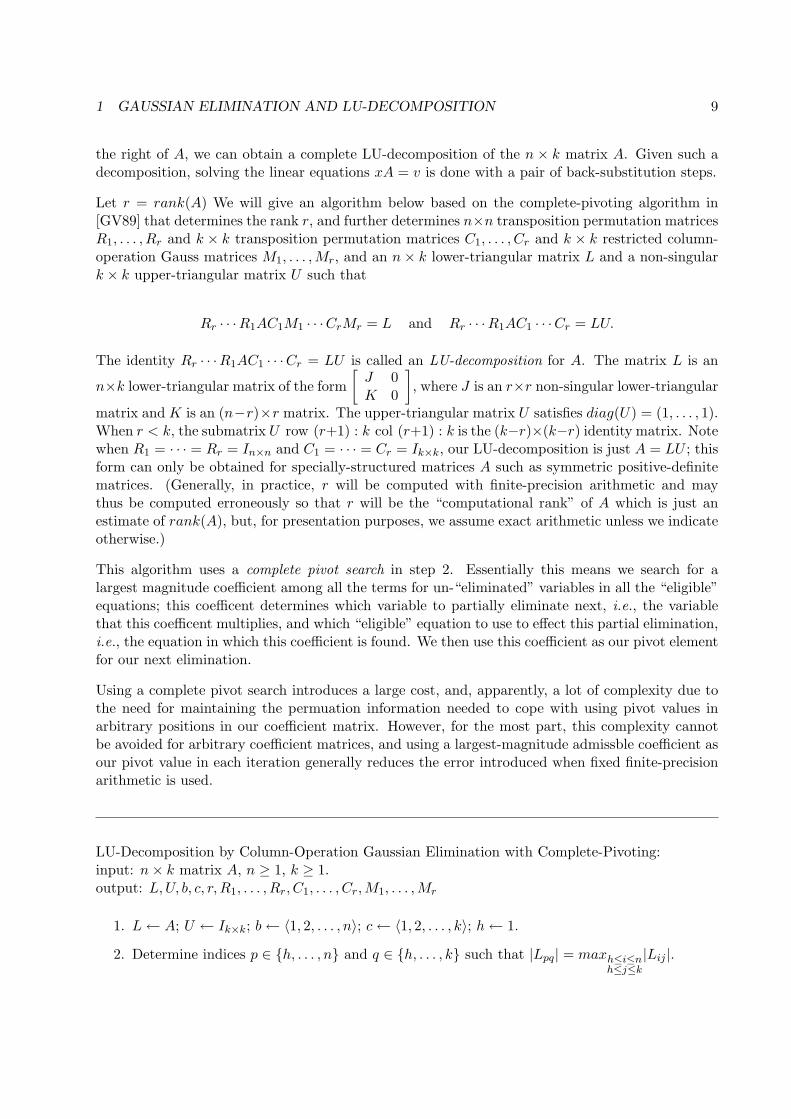
the right of A, we can obtain a complete LU-decomposition of the n × k matrix A. Given such adecomposition, solving the linear equations xA = v is done with a pair of back-substitution steps.
Let r = rank(A) We will give an algorithm below based on the complete-pivoting algorithm in[GV89] that determines the rank r, and further determines n×n transposition permutation matricesR1, . . . , Rr and k × k transposition permutation matrices C1, . . . , Cr and k × k restricted column-operation Gauss matrices M1, . . . , Mr, and an n× k lower-triangular matrix L and a non-singulark × k upper-triangular matrix U such that
Rr · · ·R1AC1M1 · · ·CrMr = L and Rr · · ·R1AC1 · · ·Cr = LU.
The identity Rr · · ·R1AC1 · · ·Cr = LU is called an LU-decomposition for A. The matrix L is an
n×k lower-triangular matrix of the form
[
J 0K 0
]
, where J is an r×r non-singular lower-triangular
matrix and K is an (n−r)×r matrix. The upper-triangular matrix U satisfies diag(U) = (1, . . . , 1).When r < k, the submatrix U row (r+1) : k col (r+1) : k is the (k−r)×(k−r) identity matrix. Notewhen R1 = · · · = Rr = In×n and C1 = · · · = Cr = Ik×k, our LU-decomposition is just A = LU ; thisform can only be obtained for specially-structured matrices A such as symmetric positive-definitematrices. (Generally, in practice, r will be computed with finite-precision arithmetic and maythus be computed erroneously so that r will be the “computational rank” of A which is just anestimate of rank(A), but, for presentation purposes, we assume exact arithmetic unless we indicateotherwise.)
This algorithm uses a complete pivot search in step 2. Essentially this means we search for alargest magnitude coefficient among all the terms for un-“eliminated” variables in all the “eligible”equations; this coefficent determines which variable to partially eliminate next, i.e., the variablethat this coefficent multiplies, and which “eligible” equation to use to effect this partial elimination,i.e., the equation in which this coefficient is found. We then use this coefficient as our pivot elementfor our next elimination.
Using a complete pivot search introduces a large cost, and, apparently, a lot of complexity due tothe need for maintaining the permuation information needed to cope with using pivot values inarbitrary positions in our coefficient matrix. However, for the most part, this complexity cannotbe avoided for arbitrary coefficient matrices, and using a largest-magnitude admissble coefficient asour pivot value in each iteration generally reduces the error introduced when fixed finite-precisionarithmetic is used.
LU-Decomposition by Column-Operation Gaussian Elimination with Complete-Pivoting:input: n× k matrix A, n ≥ 1, k ≥ 1.output: L, U, b, c, r, R1, . . . , Rr, C1, . . . , Cr, M1, . . . , Mr
1. L← A; U ← Ik×k; b← 〈1, 2, . . . , n〉; c← 〈1, 2, . . . , k〉; h← 1.
2. Determine indices p ∈ {h, . . . , n} and q ∈ {h, . . . , k} such that |Lpq| = maxh≤i≤nh≤j≤k
|Lij |.
1 GAUSSIAN ELIMINATION AND LU-DECOMPOSITION 10
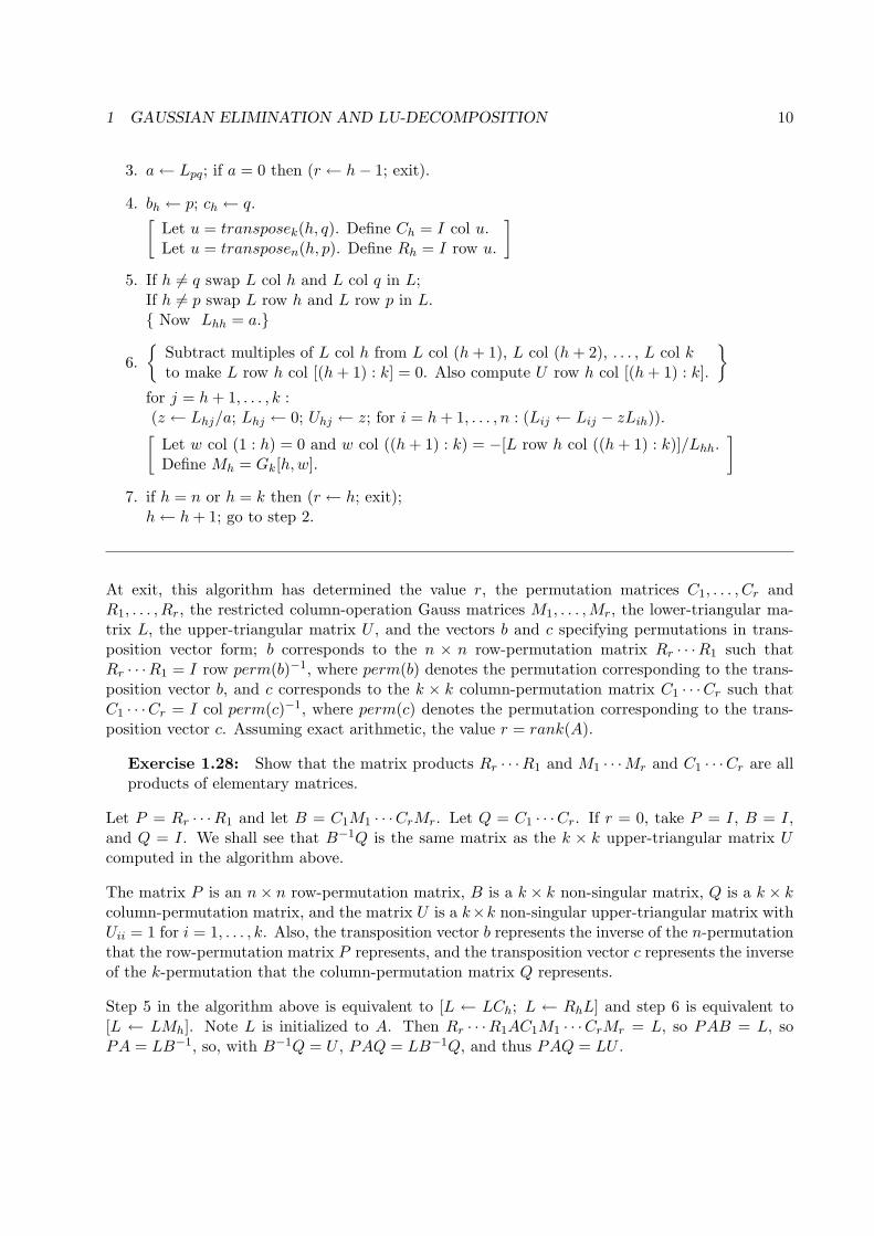
3. a← Lpq; if a = 0 then (r ← h− 1; exit).
4. bh ← p; ch ← q.[
Let u = transposek(h, q). Define Ch = I col u.Let u = transposen(h, p). Define Rh = I row u.
]
5. If h 6= q swap L col h and L col q in L;If h 6= p swap L row h and L row p in L.{ Now Lhh = a.}
6.
{
Subtract multiples of L col h from L col (h + 1), L col (h + 2), . . . , L col kto make L row h col [(h + 1) : k] = 0. Also compute U row h col [(h + 1) : k].
}
for j = h + 1, . . . , k :(z ← Lhj/a; Lhj ← 0; Uhj ← z; for i = h + 1, . . . , n : (Lij ← Lij − zLih)).[
Let w col (1 : h) = 0 and w col ((h + 1) : k) = −[L row h col ((h + 1) : k)]/Lhh.Define Mh = Gk[h, w].
]
7. if h = n or h = k then (r ← h; exit);h← h + 1; go to step 2.
At exit, this algorithm has determined the value r, the permutation matrices C1, . . . , Cr andR1, . . . , Rr, the restricted column-operation Gauss matrices M1, . . . , Mr, the lower-triangular ma-trix L, the upper-triangular matrix U , and the vectors b and c specifying permutations in trans-position vector form; b corresponds to the n × n row-permutation matrix Rr · · ·R1 such thatRr · · ·R1 = I row perm(b)−1, where perm(b) denotes the permutation corresponding to the trans-position vector b, and c corresponds to the k × k column-permutation matrix C1 · · ·Cr such thatC1 · · ·Cr = I col perm(c)−1, where perm(c) denotes the permutation corresponding to the trans-position vector c. Assuming exact arithmetic, the value r = rank(A).
Exercise 1.28: Show that the matrix products Rr · · ·R1 and M1 · · ·Mr and C1 · · ·Cr are allproducts of elementary matrices.
Let P = Rr · · ·R1 and let B = C1M1 · · ·CrMr. Let Q = C1 · · ·Cr. If r = 0, take P = I, B = I,and Q = I. We shall see that B−1Q is the same matrix as the k × k upper-triangular matrix Ucomputed in the algorithm above.
The matrix P is an n× n row-permutation matrix, B is a k × k non-singular matrix, Q is a k × kcolumn-permutation matrix, and the matrix U is a k×k non-singular upper-triangular matrix withUii = 1 for i = 1, . . . , k. Also, the transposition vector b represents the inverse of the n-permutationthat the row-permutation matrix P represents, and the transposition vector c represents the inverseof the k-permutation that the column-permutation matrix Q represents.
Step 5 in the algorithm above is equivalent to [L ← LCh; L ← RhL] and step 6 is equivalent to[L ← LMh]. Note L is initialized to A. Then Rr · · ·R1AC1M1 · · ·CrMr = L, so PAB = L, soPA = LB−1, so, with B−1Q = U , PAQ = LB−1Q, and thus PAQ = LU .
1 GAUSSIAN ELIMINATION AND LU-DECOMPOSITION 11
The relation PAQ = LU is called an LU-decomposition for A. Given PAQ = LU , we may determineif the set of linear equations xA = v is consistent, and if so, compute x such that xA = v as follows.
Note A = P−1LUQ−1 = PTLUQT since the inverse of a permutation matrix is its transpose.Then xA = v implies xPTLUQT = v implies xPTLU = vQ. Let y = xPTL. Then yU = vQ.Since U is non-singular and upper-triangular, we can compute y with back-substitution. Now recally = xPTL. Let z = xPT. Then y = zL.
If n = k and the lower-triangular matrix L is non-singular, we can compute z with back-substitution.
Otherwise, recall L is an n × k lower-triangular matrix with L =
[
J 0K 0
]
where J is an r × r
non-singular lower-triangular matrix and K is an (n − r) × r matrix. If y col [(r + 1) : k] 6= 0,our equations are inconsistent and x does not exist, (since y = zL and z[L col (r + 1) : k] = 0.)Otherwise we may take zr+1 = zr+2 = · · · = zn = 0 and solve for z1, . . . , zr in the triangular systemof linear equations [z col 1 : r]J = [y col 1 : r] via back-substitution. Now z is determined, nomatter what the value of r is.
Finally, we must appropriately permute the components of z = xPT according to the permutationmatrix P to obtain x = zP . (In order to compute zP within z, we may use the following algorithm.[for i = r, r − 1, . . . , 1: swap zi with zbi
]. Also, in order to compute vQ within v, we may use thealgorithm: [ for i = 1, 2, . . . , r: swap vi with vci
].) Here b and c are the transposition vectorscomputed in the Gaussian-elimination LU-decomposition algorithm.
Exercise 1.29: Why is the recipe for computing zP different from the recipe for comput-ing vQ? Hint: P = Rr · · ·R1 and Q = C1 · · ·Cr where Ri = I row transposen(i, bi) andCj = I col transposek(j, cj). We have zP = z(I row perm(b)−1) = z(I col perm(b)) andvQ = v(I col perm(c)−1).
Exercise 1.30: Show that bi ≥ i for i = 1, . . . , n and cj ≥ j for j = 1, . . . , k.
We could construct permutation vectors b and c representing the matrices P and Q, rather than con-structing transposition vectors as is done in step 4 in the Gaussian-elimination LU-decompositionalgorithm. We would do this by replacing ‘bh ← p’ with ‘Swap bh with bp’ and replacing ‘ch ← q’with ‘Swap ch with cq’. This defines b and c as products of transpositions, with P = I row b andQ = I col c. Then PW is computed as W row b, WP is computed as W col b−1, V Q is computedas V col c, and QV is computed as V row c−1, where W and V are arbitrary conformable matrices.
Exercise 1.31: How do we compute PTW , WPT, V QT, and QTV for conformable matricesW and V , given that the vectors b and c are permutation vectors that correspond to the row-permutation matrix P and the column-permutation matrix Q with P = I row b and Q = I col c?Hint: P−1 = PT and Q−1 = QT.
Exercise 1.32: Show that xPTL = vB, and hence zL = vB where B = QU−1.
Exercise 1.33: What is computed in the Gaussian-elimination LU-decomposition algorithmwhen the n× k matrix A = 0? What is computed when k = 1 and A = eT
n? What is the resultof the Gaussian-elimination LU-decomposition algorithm when n ≥ k? What is the result whenn < k?
1 GAUSSIAN ELIMINATION AND LU-DECOMPOSITION 12
Exercise 1.34: What is the LU-decomposition of the n× k rank 0 matrix On×k?
Exercise 1.35: What is computed in the Gaussian-elimination LU-decomposition algorithmwhen the n× k matrix A is diag(v1, v2, . . . , vmin(n,k)) where vi ∈ R for i = 1, . . . ,min(n, k)?
Exercise 1.36: If we have the same number of equations as unknowns, do we always havea solution for our linear equations xA = v? Show that if n = k and rank(A) = k, the linearequations xA = v are necessarily consistent and have a unique solution.
Exercise 1.37: Explain why U row (r + 1) : k col (r + 1) : k = Ik−r,k−r when r < k.
Exercise 1.38: Given the n×k matrix A, let m = max(n, k) and define the “augmented”m×mmatrix S as Sij = Aij for 1 ≤ i ≤ n and 1 ≤ j ≤ k, and Sij = 0 for n + 1 ≤ i ≤ m ork +1 ≤ j ≤ m. Explain how we can compute an LU-decomposition of the n×k matrix A, givenan LU-decomposition of S. This is equivalent to only using our LU-decomposition algorithmfor square matrix inputs.
Exercise 1.39: The pivot value a computed in each iteration of the Gaussian-eliminationLU-decomposition algorithm is the value of an element of L, Lpq, called the pivot element ofthat iteration. Why do we seek the largest magnitude element of L row (h : n) col (h : k) instep 2 to serve as the pivot element in iteration h? Would determining any non-zero element ofL row (h : n) col (h : k) suffice?
Solution 1.39: With exact arithmetic there is no need to seek a large pivot value; any non-zerovalue will suffice. However, with fixed finite-precision floating-point arithmetic, each arithmeticoperation may introduce error in the result, depending upon the input values. In particular, ifwe have two non-zero floating-point values b = 2rf and c = 2sg, where f and g are p-bit binaryfractions with .5 ≤ |f | < 1 and .5 ≤ |g| < 1, and r and s are integers, then, assuming overflow orunderflow does not occur, the floating-point approximation to the product bc is 2r+sfg(1 + ǫu)where |ǫ| ≤ .5 and u = 21−p; u is called the rounding-unit of our floating-point number system;u is the least positive value such that 1 + u rounded to a floating-point value with p bits ofprecision is greater than 1. (On a 64-bit IEEE floating-point machine, u = 2−52.)
The error introduced in the product is thus 2r+sfgǫu = bcǫu. The larger the magnitude of theproduct bc is, the larger the magnitude of the error can be.
Also, if b and c are themselves rounded-off results of floating-point computations of the formb = 2rf(1+βu) and c = 2sg(1+γu) for some values β and γ, not necessarily less than .5, then thefloating-point form of the product bc is 2r+sfg(1+βu)(1+γu)(1+ǫu) ≈ 2r+sfg(1+(β+γ+ǫ)u),so the error is approximately 2r+sfg(β + γ + ǫ)u. Thus error is propagated and its magnitudeis magnified as our computation progresses.
The basic computation in Gaussian-elimination LU-decomposition is of the form Lij ← Lij −(Lhj/a)Lih. When Lhj 6= 0, the smaller the magnitude of the pivot value a is, the larger themagnitude of the multiplier Lhj/a is, and hence the larger the absolute error in Lhj/a can be.And when Lih 6= 0, the error in the product (Lhj/a)Lih is a combination of the error in Lhj/aand Lih, magnified by their opposite factors, and this error propagates, increasing superlinearlyin each iteration. This is why we want to avoid using small pivot values!
1 GAUSSIAN ELIMINATION AND LU-DECOMPOSITION 13
There is also a more subtle source of error that occurs in computing the difference Lij −(Lhj/a)Lih (which is also slightly alleviated by avoiding small pivot values.)
Think about the round-off error in computing a difference of the form α− γβ
awith fixed finite-
precision arithmetic where a is a pivot value and α, β, and γ are random values. Ifγβ
a,
computed with fixed finite-precision arithmetic, is about the same size as α and has the same
sign, the difference will then suffer a large loss in precision, in which the error present inγβ
ais
magnified. By “loss of precision” we mean that α−(α− γβ
a) computed with fixed finite-precision
floating-point arithmetic is very different fromγβ
a.
Essentially, ifγβ
ais represented by
γβ
a(1+ǫu), then our computation results in
[
α− γβ
a(1 + ǫu)
]
(1+ δu) ≈ α− γβ
a− γβ
aǫu+
(
α− γβ
a
)
δu where |δ| ≤ .5, and if α− γβ
ais small, the magnitude
of the absolute error |γβ
aǫ−
(
α− γβ
a
)
δ|u can be comparatively large. When α− γβ
ais small,
the absolute error is approximately |γβ
aǫ|u, and the relative error |γβ
aǫ|u/|
(
α− γβ
a
)
| in our
result can be large. Thus we see that it is computing sums of values of similar magnitudes andopposite signs that risk causing subsequent catastophic loss-of-precision error. Loss-of-precisionerror is essentially relative error, in contrast to the absolute error discussed before.
Choosing a to be larger than an “average” value means that, more often than not,γβ
ais smaller
than average and the difference α − γβ
ahas less loss of precision than would be expected on
average. See [Knu97] for a discussion of floating-point arithmetic and round-off error.
Exercise 1.40: Show that Rt = I row transposen(t, bt) and Ct = I col transposek(t, ct) whereb and c are the transposition vectors computed in the Gaussian-elimination LU-decompositionalgorithm. Also show that Ct = CT
t = C−1t and Rt = RT
t = R−1t .
Exercise 1.41: Let p = perm(b) and let q = perm(c). Show that the transposition vectors band c computed in the algorithm above determine the row-permutation matrix P = Rr · · ·R1
such that P = I row p−1 and determine the column-permutation matrix Q = C1 · · ·Cr suchthat Q = I col q−1 respectively. Thus the matrices P and Q need not be explicitly computed.
Solution 1.41:
We have P = RrRr−1 · · ·R1 = (I row transposen(r, br)) · · · (I row transposen(1, b1)) =I row (transposen(r, br) · · · transposen(1, b1)) = I row p−1 where the permutation p corre-sponds to the transposition vector b = [b1, b2, . . . , bn] with p = transposen(1, b1) · · · transposen(r, br)= transposen(r, br) ↓ · · · ↓ transposen(1, b1). (Recall u ↓ v = uv = 〈uv1
, uv2, . . . , uvn〉.)
Thus the matrix P is the n × n row-permutation matrix I row p−1 where the n-permutation
1 GAUSSIAN ELIMINATION AND LU-DECOMPOSITION 14
p is determined by the transposition vector b via the algorithm: [p ← 〈1, 2, . . . , n〉: for i =r, r− 1, . . . , 1: swap pi with pbi
] and the n-permutation p−1 is then computed via the algorithm:[for i = 1, 2, . . . , n: p−1
pi← i].
We have Q = C1C2 · · ·Cr = (I col transposek(1, c1)) (I col transposek(1, c2)) · · ·(I col transposek(r, cr)) = I col (transposek(r, cr) · · · transposek(1, c1)) = I col q−1 where thepermutation q corresponds to the transposition vector c = [c1, c2, . . . , cn] with q = transposek(1, c1)· · · transposek(r, cr) = transposek(r, cr) ↓ · · · ↓ transposek(1, c1).
Thus the matrix Q is the k × k column-permutation matrix I col q−1 where the k-permutationq is determined by the transposition vector c via the algorithm: [q ← 〈1, 2, . . . , k〉: for i =r, r− 1, . . . , 1: swap qi with qci
] and the k-permutation q−1 is then computed via the algorithm:[for i = 1, 2, . . . , k: q−1
qi← i].
Exercise 1.42: Let p be an n-permutation and let q be a k-permutation. Show thatz(I row p−1) = z col p and v(I col q−1) = v col q−1.
Exercise 1.43: Show that Jii 6= 0 for 1 ≤ i ≤ r and show that L is non-singular if and onlyif n = k = r and L = J .
Exercise 1.44: Show that if n = k then det(A) = L11 · L22 · · ·Lnn · det(P ) · det(Q). Note,det(P )·det(Q) is either 1 or −1. If we keep track of the number, tp, of non-identity transpositionsrecorded in the transposition vectors b and c, we can determine the value of det(P ) · det(Q) as2 · (tp mod 2)− 1.
Exercise 1.45: Is R1 = · · · = Rr = I equivalent to R1 · · ·Rr = I? Is C1 = · · · = Cr = Iequivalent to C1 · · ·Cr = I?
Exercise 1.46: Show that each of the restricted Gauss matrices M1, . . . , Mr computed in theGaussian-elimination LU-decomposition algorithm is an upper-triangular matrix.
Note in practical application, none of the matrices C1, . . . , Cr, R1, . . . , Rr, or M1, . . . , Mr need tobe computed. They are effectively replaced by b, c, and U . Thus none of the bracketed operationsin the LU-decomposition algorithm need to be done!
Exercise 1.47: Show that |Uij | ≤ 1 for 1 ≤ i < j ≤ k. Hint: complete-pivoting implies thatthe value z in step 6 of the Gaussian-elimination LU-decomposition algorithm is no greater inmagnitude than 1.
Exercise 1.48: When finite-precision floating-point arithmetic operations are used, the com-puted rank r may be in error. Is the computed value r more likely to be an underestimate or anoverestimate? What is the probability that r is correct under suitable randomness assumptions?
Exercise 1.49: Let A be an n× n non-singular matrix. Show that the Gaussian-eliminationLU-decomposition algorithm with complete-pivoting applied to the matrix A chooses pivot ele-ments such that no two pivot elements lie in the same row or in the same column of A or anyiteration instance of the matrix L derived iteration-by-iteration from A.
1 GAUSSIAN ELIMINATION AND LU-DECOMPOSITION 15
It remains to demonstrate that the matrix U computed in the Gaussian-elimination LU-decompositionalgorithm is the same as the matrix B−1Q. We have
B−1Q = (C1M1C2M2 · · ·CrMr)−1C1C2 · · ·Cr = M−1
r C−1r M−1
r−1C−1r−1 · · ·C−1
2 M−11 C−1
1 C1C2 · · ·Cr,
or equivalently,
B−1Q = M−1r (Cr(M
−1r−1(Cr−1(· · · (C3(M
−12 (C2M
−11 C2))C3)) · · ·))Cr).
Recall that Ci = C−1i = CT
i is a k × k permutation matrix corresponding to a transpositiontransposek(i, j) where i ≤ j ≤ r.
Now, let wh be the k-vector such that Mh = I + eTh wh. Recall that M1, M2, . . . , Mr are restricted
Gauss matrices. For h = 1, . . . , r, we have (wh) col 1 : h = 0 and (wh) col ((h + 1) : k) =−[L row h col ((h + 1) : k)]/Lhh as computed in step 6. Then M−1
h = I − eTh wh.
Now C2M−11 C2 = C2(I − eT
1 w1)C2 = C2IC2− (C2eT1 )(w1C2) = I − eT
1 (w1C2). This follows becausethe row-permutation matrix C2 exchanges row 2 with row j where j ≥ 2, so that C2e
T1 = eT
1 . And,C2 = C−1
2 , so C2IC2 = I.
Also note that since the column-permutation matrix C2 exchanges column 2 with column j wherej ≥ 2, we have w1C2 col 1 = (w1) col 1; thus (w1) col 1 remains 0 and I − eT
1 (w1C2) remains arestricted Gauss matrix.
Next, M−12 (C2M
−11 C2) = (I−eT
2 w2)(I−eT1 (w1C2)) = I−eT
1 (w1C2)−eT2 w2, since eT
2 w2eT1 (w1C2) =
Ok×k. And thus, C3(M−12 (C2M
−11 C2))C3 = I − eT
1 (w1C2C3)− eT2 (w2C3).
Continuing in this manner, we finally obtain
B−1Q = I −∑
1≤i≤r
eTi (wiCi+1 · · ·Cr).
But, [wiCi+1 · · ·Cr] col (1 : i) = 0 and [wiCi+1 · · ·Cr] col ((i + 1) : k) is the final value ofU row i col ((i+1) : k) computed in the Gaussian-elimination LU-decomposition algorithm above.Thus B−1Q = U , where U row i = ei + wiCi+1 · · ·Cr. [QED]
Exercise 1.50: Show that U is a k × k upper-triangular matrix, and show that diag(U) =(1, . . . , 1).
When we have obtained r and L and U and P (or equivalently b) and Q (or equivalently c) such thatPAQ = LU , we can use the process described above to solve xA = v for any given righthand-sidevector v that admits a solution with two back-substitution steps, and two vector permutations.
Algorithmically, the process to solve xPTLUQT = v is:
1. Compute v ← vQ by permuting v according to the inverse of the permutation determined bythe transposition vector c.
2. Compute y such that yU = v by back-substitution.
1 GAUSSIAN ELIMINATION AND LU-DECOMPOSITION 16
3. If y col [(r + 1) : k] 6= 0 then (‘xA = v’ is inconsistent; exit.)
4. z col [(r + 1) : n]← 0.
5. Compute [z col (1 : r)] such that [z col (1 : r)][L row (1 : r) col (1 : r)] = [y col (1 : r)] viaback-substitution.
6. Compute x← zP by permuting z according to the permutation determined by the transpositionvector b.
7. exit.
In detail, this is:
1. for i = 1, 2, . . . , r: swap vi with vci.
2. for i = 1, 2, . . . , k : (yi ← vi; for j = 1, . . . , i− 1 : (yi ← yi − Ujiyj)).
3. If y col [(r + 1) : k] 6= 0 then (‘xA = v’ is inconsistent; exit.)
4. z col [(r + 1) : n]← 0.
5. for i = r, r − 1, . . . , 1 : (zi ← yi; for j = i + 1, . . . , r : (zi ← zi − Ljizj); zi ← zi/Lii).
6. x← z; for i = r, r − 1, . . . , 1: swap xi with xbi.
7. exit.
Note this algorithm destroys the input righthand-side vector v.
Exercise 1.51: Why does the loop in step 1 run for i = 1, . . . , r rather than i = 1, . . . , k?
Exercise 1.52: Can you revise the above algorithm to permute v into the vector y duringstep 2 and both prevent destroying v and save some small amount of computation?
Exercise 1.53: Show that we can dispense with the vector z in the algorithm above.
Exercise 1.54: Use the fact that U row (r + 1) : k col (r + 1) : k = I to show that step 2 canbe written as: for i = 1, 2, . . . , k : (yi ← vi; for j = 1, . . . ,min(i− 1, r) : (yi ← yi − Ujiyj)).
Exercise 1.55: Explain step 3.
Solution 1.55: When r < k, our k equations are linearly-dependent if they are consistent.In this case, L col [(r + 1) : k] = On×(k−r), so the equations zL = y are not satisfiable ify col [(r+1) : k] is not 0, and hence does not match the lefthand-side vector (zL) col [(r+1) : k].
Exercise 1.56: Show that Lii is never 0 in step 5.
Exercise 1.57: Give the algorithm for solving for the vector y in AyT = wT, given theLU-decomposition of the n × k matrix A and the righthand-side vector w. Here y ∈ Rk andw ∈ Rn.
1 GAUSSIAN ELIMINATION AND LU-DECOMPOSITION 17
We have seen that, given the LU-decomposition A = PTLUQT, the linear equations xA = v canbe written xPTLU = vQ and when the equations xA = v are consistent, x can be computed asx = zP where z satisfies zL = y := vQU−1. When the equations xA = v are consistent, then-vector z belongs to the solution flat yL+ + nullspace(L). Thus the solution flat of the linearequations xA = v is {xP ∈ Rn | x ∈ vQU−1L+ + nullspace(L)}.
Exercise 1.58: Recall that the n× k matrix L =
[
J 0K 0
]
where J is an r × r non-singular
lower-triangular matrix and K is an (n − r) × r matrix. Show that the k × n matrix L+ =[
J−1 00 0
]
. Hint: L+L is the projection onto rowspace([J K]).
The solution flat yL++nullspace(L) can be constructed as follows. The linear equations zL = y are
just the linear equations (z1 z2)
[
J 0K 0
]
= (y1 0) where z = (z1 z2), y = (y1 0), z1 is an r-vector,
z2 is an (n − r)-vector, J is an r × r non-singular lower-triangular matrix, K is an (n − r) × r
matrix, and y1 is an r-vector. Altogether the matrix
[
J 0K 0
]
is an n× k matrix and the vector
(y1 0) is a k-vector.
The equations zL = y reduce to z1J + z2K = y1. We can fix z2 to be any vector in Rn−r and takez1 to be the solution z1 = (y1−z2K)J−1 of the equations z1J +z2K = y1 in order to form a solutionof zL = y. This set of solutions of zL = y is {((y1− z2K)J−1 z2) ∈ Rn | z2 ∈ Rn−r} and this is thesame set as yL+ + nullspace(L) where yL+ = (y1J
−1 0) and nullspace(L) = {((−z2K)J−1 z2) ∈Rn | z2 ∈ Rn−r}. (Note (−z2KJ−1 z2)
[
J 0K 0
]
= (−z2K + z2K 0) = 0.)
Exercise 1.59: Recall that nullspace(AB) = nullspace(A) for conformable matrices A andB when the columns of B are linearly-independent. Let A be an n × k matrix with the LU-decomposition PTLUQT. Show that nullspace(A) = nullspace(L)P .
Solution 1.59: PA = LUQT, so nullspace(PA) = nullspace(L), and
nullspace(PA) = {x ∈ Rn | xPA = 0}= {xPT ∈ Rn | xPTPA = 0}= {xPT ∈ Rn | xA = 0}= nullspace(A)PT.
Thus nullspace(L)P = nullspace(A).
Exercise 1.60: Revise the back-substitution algorithm given above for computing x thatsatisfies xA = v to compute a barycentric basis for the solution flat of xA = v. Hint: takez col (r + 1) : n to be each of the (n− r)-vectors 0, e1, . . . , en−r in step 4.
If we wish to solve just the single system of equations xA = v, we may save some time by appendingv to A as A row (n+1), and then using Gaussian elimination (with pivot positions and values in A)
to convert the augmented matrix
[
Av
]
to lower-triangular form
J 0K 0w u
where the row [w u] is
1 GAUSSIAN ELIMINATION AND LU-DECOMPOSITION 18
the result of processing v with the Gaussian elimination steps applied to the columns of
[
Av
]
, and
then using one back-substitution step to compute x; indeed this is often what is meant by Gaussianelimination. The vector [w u] is equal to the vector y computed in step 2 in the back-substitutionprocedure above. (Does this idea, in fact, save any time?)
Exercise 1.61: Show that the equations xA = v are inconsistent if and only if rank(A) 6=rank
([
Av
])
.
Exercise 1.62: We have PAQ = LU where the n × k matrix L =
[
J 0K 0
]
and the k × k
matrix U =
[
Z W0 I
]
where J is an r × r non-singular lower-triangular matrix, K is an
(n−r)×r matrix, Z is an r×r non-singular upper-triangular matrix with diag(Z) = (1, . . . , 1),W is an r × (k − r) matrix, and I denotes an (n − r) × (n − r) identity matrix. Show that
PAQ = LU where L =
[
JK
]
and U =[
Z W]
.
Using the result of the above exercise we may re-examine solving the linear equations xA = v. We
have PAQ = LU where L =
[
JK
]
and U =[
Z W]
as described above. Let z = xPT and
w = vQ. Then xA = v is equivalent to zLU = w, and thus z
[
JK
]
[
Z W]
= w.
Therefore z
[
JZ JWKZ KW
]
= w. Now write z = [z1 z2] where z1 ∈ Rr and z2 ∈ Rn−r. Then
[z1 z2]
[
JZ JWKZ KW
]
= [z1JZ + z2KZ z1JW + z2KW ] = w.
Since rank(A) = rank(JZ) = r, when we take z2 = 0 we have z1JZ = w col 1 : r and z1JW =w col (r + 1) : k, and if these two vector equations are inconsistent, i.e., if the latter relation failsto hold given the former, the linear equations xA = v are inconsistent. Otherwise z1 = (w col 1 :r)(JZ)−1 and (w col 1 : r)Z−1W = w col (r + 1) : k and [z1 0]P = x.
It is common to use the number of floating-point arithmetic operations (flops) as a measure of thecost of a numerical algorithm.
The loop-structure of the version of the Gaussian-elimination LU-decomposition algorithm givenabove, not including the optional steps in brackets, is:
[ for h = 1, . . . , m : { for i = h + 1, . . . , k : { 1 flop }; for j = h + 1, . . . , n : { 2 flops }}]where m = min(n, k). If m = k, the outer-loop is effectively [h = 1, . . . , m − 1]. If k > n, theinner-loop: [j = h + 1, . . . , n] is empty when h = m, and there are just k − n flops used in theh = m iteration.
Thus the total cost in flops, C, for the Gaussian-elimination LU-decomposition algorithm applied
1 GAUSSIAN ELIMINATION AND LU-DECOMPOSITION 19
to a rank m n× k matrix is:∑
1≤h≤m−1
∑
h+1≤i≤k
1 +∑
h+1≤j≤n
2
+ δmn(k − n).
And thus,
C =∑
1≤h≤m−1
k − h +∑
h+1≤i≤k
2(n− h)
+ δmn(k − n)
=∑
1≤h≤m−1
[k − h + 2(n− h)(k − h)] + δmn(k − n)
=∑
1≤h≤m−1
[
(1 + 2n)k + 2h2 − h(1 + 2n + 2k)]
+ δmn(k − n)
= (1 + 2n)k(m− 1) + 2
∑
1≤h≤m−1
h2
−
∑
1≤h≤m−1
h
(1 + 2n + 2k) + δmn(k − n)
= (1 + 2n)k(m− 1) + 2
[
m3
3− m2
2+
m
6
]
− 1
2m(m− 1)(1 + 2n + 2k) + δmn(k − n)
= (1 + 2n)k(m− 1) +
[
2
3m3 −m2 +
1
3m
]
− 1
2(m2 −m)(1 + 2n + 2k) + δmn(k − n).
When n = k = m, we have C = 23m3 − 1
2m2 − 16m. (Can you explain why 2
3m3 − 12m2 − 1
6m isalways a non-negative integer when m ∈ Z+? (Other than the fact that it is a count of operations.)Is it sufficient to consider m ∈ {0, 1, 2, 3, 4, 5}?)
Note the number of flops used is not a very good indicator of the total cost of the Gaussian-elimination LU-decomposition algorithm, since there is a substantial cost in searching for a maximal-magnitude pivot element in each iteration.
Exercise 1.63: What is the maximum number of times we read an element of the matrix L,given as a function of n and k, in the Gaussian-elimination LU-decomposition algorithm above,not including the optional steps in brackets?
Solution 1.63: Let m = min(n, k). Then the maximum number of L-reads is:∑
1≤h≤m
[(n− h + 1)(k − h + 1) + 1 + 2n + 2k + (k − h)(1 + 2(n− h))] =
m3 + 32(k − n + 2)m2 + 3[(n + 2)(k + 1
2)− 16k]m.
(When n = k = m, this is 4m3 + 10m2 + 3m.)
Exercise 1.64: How should we modify the Gaussian-elimination LU-decomposition algorithmto apply to matrices and vectors with complex elements?
There are several modifications to the Gaussian-elimination LU-decomposition algorithm givenabove that are practically desirable in a computer program.
The first issue has to do with dividing by Lkk (i.e., by a). Because of the possibility of computingtoo-large or too-small values in various computations in the Gaussian-elimination LU-decomposition
1 GAUSSIAN ELIMINATION AND LU-DECOMPOSITION 20
algorithm or in a back-substitution algorithm, we should use an overflow handler that either sub-stitutes the largest representable correctly-signed value in place of the unrepresentable overflowingvalue (with a warning,) or declares our coefficient matrix to be indecomposable. Also, we shoulduse a machine with “soft” (unnormalized) underflow.
Because of round-off error the test “a = 0” in step 3 that protects us from dividing by zeromight usefully be replaced by “|a| < α”, where α is a small value. What “small” should be is acomplicated matter. A choice independent of the elements of the matrix A might be the rounding-unit u of our computer. (Recall that the rounding-unit u is the smallest value such that 1 < 1 + uin floating-point, and the “binary-precision” p is the number of bits used to represent numbersin the interval [.5, 1); p = 1 − log2(u).) Really we should take α to be a value relative to themagnitude of the numbers that produced a so that α represents the error in a; a compromise might
be α = u ·
max1≤i≤n1≤j≤k
|Aij |
/(nk), or even better, u times the average absolute value of the non-zero
elements of A. We could compute this value during the first pivot search in our LU-decompositionalgorithm.
If a is a value near the smallest normalized positive value, ǫ, of the machine then an overflow islikely to occur before too long. (For 64-bit IEEE floating-point format, ǫ = 2−1022.) When a issmall, it is hard to know if a is an “approximation of zero” or not; this is another reason we want todo a pivot search in order to avoid small pivot values whenever possible. (There is a costly devicecalled interval arithmetic that can be employed; with interval arithmetic we can know whether acomputed value could be zero if it were computed exactly.)
Note that the errors that arise in the various values of a and the other elements of L due to round-off error means that the resulting elements of L and U are likely to be incorrect and the computedvalue of the rank of A may be incorrect. Suppose rank(A) = r. Due to round-off error, it can beunlikely that we will see Ljj = 0 for j = r + 1, . . . , min(n, k). The best we can do using Gaussianelimination with ordinary floating-point arithmetic is to estimate the rank of A by treating finalsmall absolute values of diag(L) as zero.
Exercise 1.65: Will it always be the case that Ljj 6= 0 for j = 1, . . . , rank(A) whenthe Gaussian-elimination LU-decomposition algorithm is executed with fixed finite-precisionfloating-point arithmetic?
In some cases we want to enforce a requirement that the n×k matrix A be of full-rank: rank(A) =min(n, k). We can modify A if necessary to do this. In this circumstance, we may replace thestatement “if a = 0 then (r ← h−1; exit)” in step 3 with “if |a| < ε then {a← Sign(a)(|a|+2·m)}”,where Sign(a) = 1 if a ≥ 0 and Sign(a) = −1 otherwise, and where m is a small positive value[PTVF92]. (We may also want to issue a warning or set a flag to indicate when this modificationoccurs.) Suitable choices for m might be the value 100ε or ε+minAij 6=0 |Aij |/100. (What is a suitablechoice for ε?) This device of forcing A to have full-rank is also a “stabilization” device since addingsuitable constants to each diagonal element of an n×n matrix to force it to be non-singular usuallyimproves its “condition” for processing by the Gaussian-elimination LU-decomposition algorithm.
The second issue has to do with the cost of searching for a pivot element. The Gaussian-eliminationLU-decomposition algorithm given above processes the columns of A one-by-one; The processing of
1 GAUSSIAN ELIMINATION AND LU-DECOMPOSITION 21
a single column consists of permuting the eligible rows and columns of A to bring a non-zero valueto the diagonal position in the column being processed (i.e., for column j, the diagonal position isrow j of column j,) and then subtracting multiples of this column from other columns to “zero-out”the row or “tail” of the row of that diagonal position.
In each iteration, the non-zero diagonal element holding our pivot value, after permuting to bring itinto the diagonal, (denoted by a in the Gaussian-elimination LU-decomposition algorithm,) is calledthe pivot element in that iteration, and the process of “zeroing-out” or eliminating elements in thepivot-element row is called elimination, specifically the process of “zeroing-out” (“eliminating”) theelements in the pivot-element row following the pivot-element itself is called tail-elimination,) sothe Gaussian-elimination LU-decomposition algorithm consists of min(n, k) or fewer tail-eliminationoperations. (In general, in contrast to a tail-elimination step, a single full-elimination step appliedto a matrix A with respect to the pivot element Aij is generally taken to be just the transformationeffected by the post- or pre-multiplication of A by the appropriate (non-restricted) Gauss matrixthat converts A row i to ej , or alternately A col j to eT
i when a “transposed” form of Gaussianelimination is used.)
In step 2 of the Gaussian-elimination LU-decomposition algorithm, the search for the element withthe largest absolute value in the sub-array L row [h : n] col [h : k] is called a complete pivot search,(or just complete-pivoting,) and the element Lpq = a that is found is the pivot element at iteration h.Using the element with the largest absolute value generally results in the best numerical “stability”– we generally obtain close to the least practicable error in the resulting solution vector or vectorscomputed based on the lower-triangular matrix L. Complete pivot searching is time-consuming.Nevertheless, in order to sucessfully terminate and to guarantee the exact form of the matrix Lspecified above in the case of a singular matrix, and even for many non-singular matrices, we needsome sort of pivot search; we must, at least, search for a non-zero element.
Exercise 1.66: If the matrix A has non-zero diagonal elements A11, A22, . . . , Amm wherem = min(n, k), is it necessary to use a pivot search in constructing the LU-decomposition of A?That is, can the h-th diagonal element of L as modified in the prior iteration serve as the pivotelement in iteration h?
Exercise 1.67: Can we really guarantee we will get a close approximate solution to xA = v inthe case where A is non-singular by using the LU-decomposition algorithm given above, followedby two back-substitution computations done in 64-bit floating-point arithmetic?
Solution 1.67: It depends on what the meaning of ‘close approximation’ is.
When all we care about is computing the unique solution to xA = v when it exists, then thereis a practical compromise called cross-row partial pivot search, (or just cross-row partial-pivoting,)where we replace the pivot-value search in step 2 with: “Determine the index p ∈ {h, . . . , n} suchthat |Lph| = maxh≤i≤n|Lih|.”, and then take a = Lph in step 3 and drop the unnecessary unexecutedstatement “If h 6= q swap L col h and L col q in L” in step 5. A cross-row partial pivot searcheffectively searches L col h, (across the rows of L col h,) for an element of maximum magnitude.Note that if L row h : n col h = 0, our coefficient matrix A would be singular. (In fact, all ofL col h would be 0.)
Exercise 1.68: Try using cross-row partial-pivoting and back-substitution to solve the linear
1 GAUSSIAN ELIMINATION AND LU-DECOMPOSITION 22
equations [x1 + x2 + x3 = 3, x1 = 1, x2 + x3 = 2].
Much experience has shown that, for A non-singular, computing the solution to xA = v usingpartial-pivoting is almost always stable and it is much less costly than complete-pivoting. Whenthe matrix A is non-singular, partial-pivoting will usually succeed in computing an acceptableapproximation to the LU-decomposition of A.
Exercise 1.69: Show that when cross-row partial-pivoting is used, the permutation matricesC1, . . . , Cr will all be the k × k identity matrix I.
Exercise 1.70: Show that the maximum number of times we read an element of the matrixL in the LU-decomposition algorithm using cross-row partial-pivoting, as a function of n and kis: 2
3m3 − (k + n)m2 + ((2k − 1) + 13)m− 2nδmk where m = min(n, k). (When n = k = m, this
is 23m3 −m2 + 5
6m.)
We could also replace the pivot-value search in step 2 with: “Determine the index q ∈ {h, . . . , k}such that |Lhq| = maxh≤i≤k|Lhi|.”, and then take a = Lhq in step 3 and drop the unnecessaryunexecuted statement “If h 6= p swap L row h and L row p in L” in step 5. In this case, thepermutation matrices R1, . . . , Rr will all be the n × n identity matrix. We shall call this variantof partial-pivoting, cross-column partial pivot search. When A is non-singular and cross-columnpartial-pivoting is used, we have AC1M1 · · ·CrMr = L, and Lii 6= 0 for 1 ≤ i ≤ n. Note, in this case,we are, in essence, changing the basis of rowspace(A) by multiplying by the change-of-coordinatesmatrix C1M1 · · ·CrMr to obtain a “lower-triangular” basis for rowspace(A).
Exercise 1.71: Why must A be non-singular to ensure that AC1M1 · · ·CrMr = L is ob-tained with cross-column partial-pivoting? Hint: what happens in our Gaussian-eliminationLU-decomposition algorithm with a cross-column partial pivot search when a 0 pivot valuearises?
Exercise 1.72: Suppose A is a non-singular matrix so that n = k. Show that when completepivoting is used, |Lij | ≤ |Ljj | for 1 ≤ i ≤ n. Does this hold when a cross-row partial pivotsearch is used? Does this hold when a cross-column partial pivot search is used?
When cross-column partial-pivoting is applied to an n × k matrix A with rank(A) < min(n, k),as the Gaussian-elimination process progresses, (using exact arithmetic,) we will have one or morerows where the value in the pivot position in that row, position (h, j), is zero, and all the valuesLh,j+1, . . . , Lh,k are zero as well. If we just continue the Gaussian-elimination process with thenext row of L (if any,) and the same column of L, (i.e, we take Lh+1,j as the next pivot elementposition,) we will obtain a lower-triangular matrix with one or more zero diagonal elements. Thislower-triangular matrix, possibly with one or more zero diagonal elements, is called an echelon-form matrix equivalent to the matrix A. Note if a lower-triangular echelon-form matrix L hasLjj = 0 then L row j : n col j = 0. Any triangular matrix L equivalent to A gives the rank of A asmin(n, k)− (the number of 0’s in the diagonal of L). The rows of such a matrix can be permuted
to obtain a lower-triangular matrix L =
[
J 0K 0
]
with J an r × r lower-triangular non-singular
matrix.
We may modify our search for a pivot value in the sub-array L row h : n col h : k to accept
1 GAUSSIAN ELIMINATION AND LU-DECOMPOSITION 23
the first non-zero value encountered. Using the first encountered non-zero element as the pivotelement will be called minimal-pivoting. Note a pivot search is required in general, even whenrank(A) = min(n, k), since Lhh may be zero in any iteration.
There are strategies for pivot searching beyond a minimal pivot search, a cross-column or cross-rowpartial pivot search, or a complete pivot search. For example, the following strategy, called a rookpivot search, may be used [NP92].
[p← h; q ← h; a← Lhh; s← h; t← 0;α : for i = h, . . . , k : if |Lpi| > |a| then {q ← i; a← Lpi}; if t 6= q then (t← q) else exit;
for i = h, . . . , n : if |Liq| > |a| then {p← i; a← Liq}; if s 6= p then (s← p; goto α) else exit].
This code computes p, q, and a such that a = Lpq is the pivot element selected for iteration h.The selected pivot element is an element in L row h : n col h : k which is an element of maximummagnitude in both its row and its column. This pivot search strategy generally performs onlya modest amount worse than complete-pivoting with respect to introduced round-off error and isusually much less costly than complete-pivoting with an estimated average total cost of em(m−1)/2comparisons for computing all the pivot elements needed to construct an LU-decomposition of a“random” n× k matrix where m = max(n, k) [Fos97].
Exercise 1.73: Show that the rook pivot search algorithm given above always terminates.(Does this remind you of the result that a function of two variables has a maximum in anyclosed and bounded region in its domain?)
Exercise 1.74: Give an example n × n matrix where at least n2 comparisons are requiredto find an element which is both row and column maximal using rook pivot searching. (Thealgorithm given above uses 2n2 comparisons in the worst case.)
Exercise 1.75: Note that the rook pivot search algorithm above does unnecessary compar-isons. Can you find a nice way to avoid these comparisons?
Exercise 1.76: Let A be an n×k matrix with unequal elements. Show that there are at mostmin(n, k) elements of A that are both row and column maximal.
The rook pivot search algorithm, like cross-row or cross-column partial pivoting, is not guaranteedto produce a non-zero pivot value; a zero pivot value may be chosen, even when an eligible non-zeropivot value exists. This can happen when the submatrix L row h : n col h : k has L row h col h :k = 0 and L row h : n col h = 0 with h < min(n, k). We can deal with this by reverting to aminimal pivot search for a non-zero value in the situation where the rook pivot search results in azero pivot value. This is required to ensure that any n×k matrix A can be decomposed. (However,when A is non-singular, the rook pivot search algorithm, like cross-row or cross-column partialpivoting, will never fail to produce a non-zero pivot value, assuming exact arithemetic.)
Exercise 1.77: When can we avoid searching for a pivot value entirely, i.e., when can wereplace step 2 with “p← h; q ← h.”? (Does it suffice for Aii to be non-zero for 1 ≤ i ≤ n?)
Exercise 1.78: Can we save any time by searching for the next pivot value in L row ((h+1) :n) col ((h + 1) : k) while we are subtracting suitable multiples of L row ((h + 1) : n) col h from
1 GAUSSIAN ELIMINATION AND LU-DECOMPOSITION 24
L row ((h + 1) : n) col ((h + 1) : k) in step 6, and not using step 2 after the first initial pivotvalue is determined?
Solution 1.78: Probably we can obtain a constant-factor speed-up. The exact improvementdepends on how good a coder you or your compiler is. But the maximum running time of theLU-decomposition algorithm remains O(min(n, k)3).
Third and finally, by dropping the assignment “U ← Ik×k” in step 1 and replacing the commands“Lhi ← 0; Uhi ← z” with “Lhi ← z” in step 6, we can save space in the Gaussian-eliminationLU-decomposition algorithm by storing the elements Uij for 2 ≤ i < min(n, k) and i < j ≤ kin the strictly-upper-triangular part of the matrix L (which would otherwise be 0) as it is beingformed; Uii is known to be 1 for i = 1, . . . , k, Uij is known to be 0 for 2 ≤ i > j < k, andU row (n + 1 : k) = [Ok−n,n Ik−n,k−n] when n < k. Thus the k× k matrix U need not be explicitlycreated as a separate array. (Note, if we do not save U in the upper-triangle of L, then we can save alittle time by replacing the statement “Swap L col h and L col q in L” with “Swap L row h : n col hand L row h : n col q in L”.)
The “access” function for the elements of the matrix U stored in the upper-triangular part of L asdescribed above is:[U(i, j) := if (i > j) return(0) else if (i = j) return(1) else if (i > n) return(0) else return(Lij)].(This algorithm assumes 1 ≤ i ≤ k and 1 ≤ j ≤ k.)
Also note we may save space by dispensing with the assignment “L ← A” in step 1, and justoverwrite the matrix A with L and U (less the main diagonal of U) when the destruction of theinput matrix A is permissible.
Exercise 1.79: In machine language, or in a language like C with pointer data-types, we canavoid the assignment “L← A” even when A is to be preserved; this saves nk scalar assignments,although space for L is still required. We can do this by loading L with values during the firstiteration of the LU-decomposition where L row 1 col 2 : k is made zero in a manner compatiblewith using the (strict) upper triangle of L to hold the values of U . Explain in more detail howthis can be done.
Exercise 1.80: Explain how we can store an n× n lower-triangular matrix, L, in n(n + 1)/2locations: mem[0 : n(n+1)/2−1] so that we can access the matrix element Lij with the program
[if (i < j) return(0); k ← (i− 1)i
2+ j − 1; return(mem[k]).] Give the corresponding access
function for an n× n upper-triangular matrix stored in n(n + 1)/2− 1] locations.
Suppose we use a row-indexing vector ri and a column-indexing vector ci maintained so that ri[j]is the position of the original row j in the matrix L and ci[k] is the position of the original columnk in the matrix L. In order to do complete-pivoting, the rows and columns of L are exchanged instep 5 of the LU-decomposition algorithm above; instead we may just swap the appropriate entriesof the indexing vectors ri and ci, and not swap the rows and columns of L in step 5. Then weaccess the array L as Lri[j],ci[k] rather than Ljk. (With U stored in the upper-triangle of L, thisdevice also manages U appropriately.)
If, at the end of the LU-decomposition algorithm, we restore L to its final permuted state by
1 GAUSSIAN ELIMINATION AND LU-DECOMPOSITION 25
applying the permutation in ri to the rows of L and applying the permutation in ci to the columnsof L, then we save little time overall, and if computing Lri[j],ci[k] rather than Ljk costs two additionalmemory accesses (assuming the indices j and k are kept in registers and have relatively small accesscost,) then we lose time overall. However, if we never restore L (and U) to the permuted statewhere A = PTLUQT and use the indexing arrays ri and ci to access L (and U) when doing, forexample, back-substitution, then we may save some time by thus avoiding the row and columnswaps done in step 5 in the case where computing Lri[j],ci[k] rather than Ljk costs the equivalentof much less than two additional accesses; otherwise we still do not save time by using indexingarrays. (We might be able to keep the indexing arrays in fast memory for instance. Indeed, perhapsa special LU-decomposition chip would be worth designing.)
Exercise 1.81: Quantify the relative costs in using indexing arrays, and avoiding row andcolumn swapping in complete-pivoting, under various assumptions about the additional cost ofcomputing Lri[j],ci[k] rather than Ljk.
The LU-decomposition PAQ = LU for a given n× k matrix A is trivially unique in the sense thatapplication of the complete-pivoting Gaussian-elimination LU-decomposition algorithm executes aunique sequence of computations (assuming a systematic method of resolving ties in pivot searchesis used.)
The question remains as to whether there are more than one pair of lower-triangular and upper-triangular matrices L and U of the forms produced by the Gaussian-elimination LU-decompositionalgorithm such that A = PTLUQT where the permutation matrices P and Q are produced in theGaussian-elimination LU-decomposition algorithm applied to the matrix A with P and Q fixed tocorrespond to a specific admissible choice of the sequence of pivot elements.
We can see that it is plausible that this factorization is unique when n = k as follows. Letrank(A) = r. Now consider the LU-decomposition PAQ = LU with A given and the admissiblepermutation matrices P and Q fixed. We have rn − (r − 1)r/2 elements of L to be determined,and (k− 1)k/2 elements of U to be determined (remember diag(U) = (1, . . . , 1).) We have nk non-linear equations relating these rn− (r− 1)r/2+ (k− 1)k/2 values and we know these equations areconsistent. When rn−(r−1)r/2+(k−1)k/2 of our nk equations are independent, the values definingthe matrices L and U are uniquely determined. This is possible when nk ≥ rn− (r−1)r+(k−1)k,or equivalently, when 2rn− (r− 1)r ≤ 2kn− (k− 1)k. And since r ≤ min(n, k), this is always thecase when n = k. (It turns-out, however, that a sufficent number of independent equations do notgenerally exist when r < min(n, k).)
Exercise 1.82: Suppose we have two LU-decompositions: P1AQ1 = L1U1 and also P2AQ2 =L2U2. Show that P2P
T1 L1U1Q
T1 Q2 = L2U2. Explain what this means about the uniqueness of
the LU-decomposition of A.
Exercise 1.83: Show that for any fixed sequence of non-zero pivot elements determining thepermutation matrices P and Q, the LU-decomposition PAQ = LU , with diag(U) = (1, 1, . . . , 1),is unique when the matrix A is non-singular.
Solution 1.83: Suppose A is non-singular. If PAQ = L1U1 and also PAQ = L2U2 whereL1 and L2 are lower-triangular non-singular matrices and U1 and U2 are upper-triangular non-singular matrices with diag(U1) = diag(U2) = (1, . . . , 1) then L1U1 = L2U2 so L−1
2 L1 = U2U−11 .
1 GAUSSIAN ELIMINATION AND LU-DECOMPOSITION 26
And L−12 L1 is lower-triangular since the product of lower-triangular matrices is lower-triangular
and the inverse of a non-singular lower-triangular matrix is itself lower-triangular, and similarlyU2U
−11 is upper-triangular. But a matrix that is both lower-triangular and upper-triangular
is a diagonal matrix so L−12 L1 = U2U
−11 = D where D is an n × n diagonal matrix where
diag(D) = (diag(L−12 ), diag(L1)) = (diag(U2), diag(U−1
1 )).
But the diagonal of the inverse of a non-singular triangular matrix M is specified by diag(M−1) =(1/M11, 1/M22, . . . , 1/Mnn) so diag(D) = (1, . . . , 1) since diag(U2) = (1, . . . , 1) and diag(U−1
1 ) =(1, . . . , 1). Thus L−1
2 L1 = U2U−11 = I so L1 = L2 and U2 = U1, and thus, for given permutation
matrices P and Q, the LU-decomposition PAQ = LU is unique when A is non-singular andP and Q are chosen to produce non-zero pivots in the Gaussian-elimination LU-decompositionalgorithm.
Let A be an n×k rank r matrix, and consider the LU-decomposition PAQ = LU . We can transformthis relation to write QTATPT = UTLT. Note LT is upper-triangular and UT is lower-triangularwith diag(UT) = (1, . . . , 1). We can “reshape” this relation to obtain the LU-decomposition of AT
as follows.
Suppose r ≤ n ≤ k. Then LT is a k × n matrix with LT row (r + 1) : k = 0 and UT is a k × klower-triangular matrix with diag(UT) = (1, . . . , 1). Let U = LT row 1 : n; U is just LT with k−nzero-rows removed, so U is an n × n upper-triangular matrix. Let L = UT col 1 : n; L is just UT
with columns (n+1) : k removed, so L is a k×n lower-triangular matrix with diag(L) = (1, . . . , 1).Now by examining a block-multiplication, we can see that UTLT = LU .
Exercise 1.84: Write-out the block-multiplication which verifies that UTLT = LU in the casewhere r ≤ n ≤ k.
We have U =
[
JT KT
0 0
]
with U row (r + 1) : n = 0; thus we may take L col (r + 1) : n to be
0, and then take U row (r + 1) : n col (r + 1) : n to be I(n−r)×(n−r), and the product LU remains
unchanged. Now U is an n × n upper-triangular matrix with Uii 6= 0 for 1 ≤ i ≤ n, so U isnon-singular.
Now suppose r ≤ k < n. Then define the n × n upper-triangular matrix U =
[
LT
0
]
; we have
appended n−k zero-rows to LT to form U . Define the k×n lower-triangular matrix L =[
UT 0]
;
we have appended n−k zero-columns to UT to form L. Again, by examining a block-multiplication,we can see that UTLT = LU . Also we can “transfer rank” from L to U in the same way we didbefore. We can replace L col (r + 1) : k with 0, and then replace U row (r + 1) : n col (r + 1) : nwith I(n−r)×(n−r). Now we still have LU = LTUT and U is now an n× n upper-triangular matrix
with Uii 6= 0 for 1 ≤ i ≤ n, so U is non-singular. And L is a k × n lower-triangular matrix withLii = 1 for 1 ≤ i ≤ r.
Exercise 1.85: Write-out the block-multiplication which verifies that UTLT = LU in the casewhere r ≤ k < n.
Thus, whether k ≤ n or k > n, the matrix product LU satisfies the criteria for being an LU-decomposition factorization, except that we do not necessarily have diag(U) = (1, . . . , 1). But we

1 GAUSSIAN ELIMINATION AND LU-DECOMPOSITION 27
do have Uii 6= 0 for 1 ≤ i ≤ n, so we can fix our factorization as follows.
Let the n × n diagonal matrix D = diag(U). Now define L = LD and define U = D−1U . Thismakes diag(U) = (1, . . . , 1) and makes diag(L row 1 : r) = diag(D row 1 : r). Since Dii 6= 0 for1 ≤ i ≤ n, we have Lii 6= 0 for 1 ≤ i ≤ r. Also LU = LDD−1U = LU . Thus, if PAQ = LU is anLU-decomposition of A, then QTATPT = LU is an LU-decomposition of AT.
As a practical matter, for the purpose of solving non-singular systems of linear equations, we neednot insist on a particular form of LU-decomposition. The essential feature we require is just thatwe can write PAQ = LU for the matrix A where P and Q are permutation matrices and L andU are non-singular triangular matrices. When this is the case, we can solve the equations xA = vor AxT = vT by two back-substitution computations together with the associated permutationsspecified by the matrices P and Q.
Note the Gaussian-elimination LU-decomposition algorithm given above can be “transposed” andrecast to zero-out the “tail” parts of successive columns by subtracting suitable multiples of suc-cessive pivot rows. In this case, we construct an upper-triangular matrix in the (copy of the) inputmatrix A, and concommitantly construct a lower-triangular matrix of pivot-element-scaled valueswith an implicit diagonal of ones. This version of the Gaussian-elimination LU-decomposition algo-rithm performs row operations and is equivalent to multiplying A on the left by certain restrictedGauss matrices (and by pivot-positioning permutation matrices on both the left and right.) There-fore, just as in the column-operation algorithm, we obtain a factorization of the form PAQ = LU ,where it is now the matrix L that is the non-singular factor with diag(L) = (1, . . . , 1).
Exercise 1.86: Write the row-operation version of the Gaussian-elimination LU-decompositionalgorithm.
Solution 1.86:
LU-Decomposition by Row-Operation Gaussian Elimination with Complete-Pivoting:input: n× k matrix A, n ≥ 1, k ≥ 1.output: L, U, b, c, r, R1, . . . , Rr, C1, . . . , Cr, M1, . . . , Mr
1. U ← A; L← In×n; b← 〈1, 2, . . . , n〉; c← 〈1, 2, . . . , k〉; h← 1.
2. Determine indices p ∈ {h, . . . , n} and q ∈ {h, . . . , k} such that |Upq| = maxh≤i≤nh≤j≤k
|Uij |.
3. a← Lpq; if a = 0 then (r ← h− 1; exit).
4. bh ← p; ch ← q.[
Let u = transposek(h, q). Define Ch = I col u.Let u = transposen(h, p). Define Rh = I row u.
]
5. If h 6= q swap U col h and U col q in U ;If h 6= p swap U row h and U row p in U .{ Now Uhh = a.}
1 GAUSSIAN ELIMINATION AND LU-DECOMPOSITION 28
6.
{
Subtract multiples of U row h from U row (h + 1), U row (h + 2), . . . , U row nto make U col h row [(h + 1) : n] = 0. Also compute L col h row [(h + 1) : n].
}
for i = h + 1, . . . , n :(z ← Uih/a; Uih ← 0; Lih ← z; for j = h + 1, . . . , k : (Uij ← Uij − zUhj)).[
Let w col (1 : h) = 0 and w col ((h + 1) : n) = −[U col h row ((h + 1) : n)]/Uhh.Define Mh = Gn[h, w]T.
]
7. if h = n or h = k then (r ← h; exit);h← h + 1; go to step 2.
At exit, this algorithm has determined the value r, the permutation matrices C1, . . . , Cr andR1, . . . , Rr, the row-operation Gauss matrices M1, . . . , Mr, the lower-triangular matrix L, theupper-triangular matrix U , and the permutations b and c in transposition vector form thatcorrespond to the permutation matrices P = RrRr−1 · · ·R1 and Q = C1C2 · · ·Cr.
The value r is the rank of the matrix A (assuming exact arithmetic.) The matrices R1, . . . , Rr
are n × n transposition permutation matrices, the matrices C1, . . . , Cr are k × k transpositionpermutation matrices, and the matrices M1, . . . , Mr are n × n restricted row-operation Gaussmatrices.
The matrix L is a non-singular n × n lower-triangular matrix with diag(L) = (1, . . . , 1) and
the matrix U is an n × k upper-triangular matrix of the form
[
J K0 0
]
, where J is an r × r
non-singular upper-triangular matrix and K is an (k − r)× r matrix such that
MrRr · · ·M1R1AC1 · · ·Cr = U and Rr · · ·R1AC1 · · ·Cr = LU = PAQ.
As with the column-operation version, the outputs L, U , b, c, and r are the only essential outputs.Moreover, the variable part of the strictly-lower-triangular part of L can be returned in the strictlower-triangle of the matrix U , thus saving space.
Exercise 1.87: Let B = MrRr · · ·M1R1, let P = Rr · · ·R1, and let Q = C1 · · ·Cr, whereMr, . . . , M1, Rr, . . . , R1, and C1, . . . , Cr are produced by the row-operation Gaussian-eliminationLU-decomposition algorithm given above. Show that B is non-singular. Let L = PB−1. Showthat L is an n× n non-singular lower-triangular matrix with diag(L) = (1, . . . , 1).
Exercise 1.88: Give the algorithm for solving the linear system xA = v, given the row-operation LU-decomposition of the matrix A.
Exercise 1.89: Can you construct a column-operation version and a row-operation version ofthe Gaussian-elimination LU-decomposition algorithm which scan along the main-diagonal ofthe input matrix “backwards” from lower-right to upper-left?
Exercise 1.90: Let PAQ = LU be an LU-decomposition of the n× k matrix A computed bythe column-operation version of the Gaussian-elimination LU-decomposition algorithm. Show
1 GAUSSIAN ELIMINATION AND LU-DECOMPOSITION 29
that, if we apply the row-operation version of the Gaussian-elimination LU-decomposition al-gorithm to the k × n matrix AT using the same choice of pivot elements that correspond tothe row and column-permutation matrices being identical to the transposes of the column androw-permutation matrices Q and P , then the LU-decomposition we obtain is identical to thedecomposition UTLT which we considered above.
Exercise 1.91: Let G =
∏
1≤i≤ni6=r
En[r, i,−Aic]
En[r, r,−1+1
Arc], where A is an n×n matrix
with Arc 6= 0. What is the matrix product GA?
1.2 Variants of LU-Decomposition
Let m = min(n, k). Suppose the n × k matrix A satisfies rank(A) ≥ m − 1 and has its rows andcolumns “pre-permuted” so that A can be decomposed into the product LU with no pivot search,(which means the successive matrix elements Lhh computed during the LU-decomposition must benon-zero since they are used as pivot values.) We shall call such an LU-decomposition with nopermutations involved a direct LU-decomposition, and we shall call an n × k matrix whose firstmin(n, k) − 1 pivot values computed with no pivot search are non-zero a diagonal-pivot matrix.(Note a diagonal-pivot matrix may have its last pivot value equal to zero since the last pivot valuenever serves as a denominator.) When A is a diagonal-pivot matrix, the Gaussian-eliminationLU-decomposition algorithm can be written as follows (omitting the computation of the rank r.)
LU-Decomposition Gaussian Elimination with No Pivot Search:input: n× k matrix A, n ≥ 1, k ≥ 1.output: n× n lower-triangular matrix L, n× k upper-triangular matrix U , if successful.
1. L← A; U ← Ik×k; m← min(n, k).
2. for h = 1, . . . , m :for j = 1, . . . , k :for i = 1, . . . , n :if i > h and j > h then {a← Lhh; if a = 0 then exit(“0 pivot encountered.”);
z ← Lhj/a; if i = n then (Lhj ← 0; Uhj ← z); Lij ← Lij − zLih}
3. exit.
Exercise 1.92: When can the loop “for h = 1, . . . , m :” in the procedure above be replacedby “for h = 1, . . . , m− 1 :”? Hint: what if n = k?
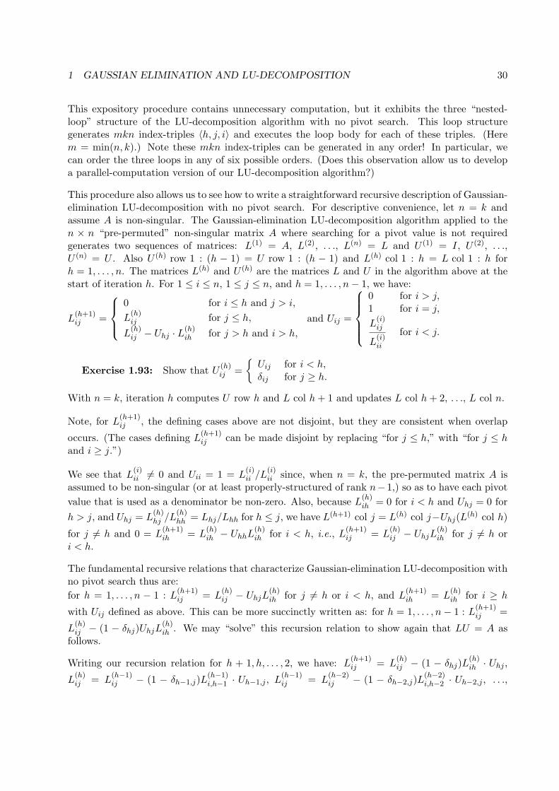
1 GAUSSIAN ELIMINATION AND LU-DECOMPOSITION 30
This expository procedure contains unnecessary computation, but it exhibits the three “nested-loop” structure of the LU-decomposition algorithm with no pivot search. This loop structuregenerates mkn index-triples 〈h, j, i〉 and executes the loop body for each of these triples. (Herem = min(n, k).) Note these mkn index-triples can be generated in any order! In particular, wecan order the three loops in any of six possible orders. (Does this observation allow us to developa parallel-computation version of our LU-decomposition algorithm?)
This procedure also allows us to see how to write a straightforward recursive description of Gaussian-elimination LU-decomposition with no pivot search. For descriptive convenience, let n = k andassume A is non-singular. The Gaussian-elimination LU-decomposition algorithm applied to then × n “pre-permuted” non-singular matrix A where searching for a pivot value is not requiredgenerates two sequences of matrices: L(1) = A, L(2), . . ., L(n) = L and U (1) = I, U (2), . . .,U (n) = U . Also U (h) row 1 : (h − 1) = U row 1 : (h − 1) and L(h) col 1 : h = L col 1 : h forh = 1, . . . , n. The matrices L(h) and U (h) are the matrices L and U in the algorithm above at thestart of iteration h. For 1 ≤ i ≤ n, 1 ≤ j ≤ n, and h = 1, . . . , n− 1, we have:
L(h+1)ij =
0 for i ≤ h and j > i,
L(h)ij for j ≤ h,
L(h)ij − Uhj · L(h)
ih for j > h and i > h,
and Uij =
0 for i > j,1 for i = j,
L(i)ij
L(i)ii
for i < j.
Exercise 1.93: Show that U(h)ij =
{
Uij for i < h,δij for j ≥ h.
With n = k, iteration h computes U row h and L col h + 1 and updates L col h + 2, . . ., L col n.
Note, for L(h+1)ij , the defining cases above are not disjoint, but they are consistent when overlap
occurs. (The cases defining L(h+1)ij can be made disjoint by replacing “for j ≤ h,” with “for j ≤ h
and i ≥ j.”)
We see that L(i)ii 6= 0 and Uii = 1 = L
(i)ii /L
(i)ii since, when n = k, the pre-permuted matrix A is
assumed to be non-singular (or at least properly-structured of rank n− 1,) so as to have each pivot
value that is used as a denominator be non-zero. Also, because L(h)ih = 0 for i < h and Uhj = 0 for
h > j, and Uhj = L(h)hj /L
(h)hh = Lhj/Lhh for h ≤ j, we have L(h+1) col j = L(h) col j−Uhj(L
(h) col h)
for j 6= h and 0 = L(h+1)ih = L
(h)ih − UhhL
(h)ih for i < h, i.e., L
(h+1)ij = L
(h)ij − UhjL
(h)ih for j 6= h or
i < h.
The fundamental recursive relations that characterize Gaussian-elimination LU-decomposition withno pivot search thus are:
for h = 1, . . . , n − 1 : L(h+1)ij = L
(h)ij − UhjL
(h)ih for j 6= h or i < h, and L
(h+1)ih = L
(h)ih for i ≥ h
with Uij defined as above. This can be more succinctly written as: for h = 1, . . . , n− 1 : L(h+1)ij =
L(h)ij − (1 − δhj)UhjL
(h)ih . We may “solve” this recursion relation to show again that LU = A as
follows.
Writing our recursion relation for h + 1, h, . . . , 2, we have: L(h+1)ij = L
(h)ij − (1 − δhj)L
(h)ih · Uhj ,
L(h)ij = L
(h−1)ij − (1 − δh−1,j)L
(h−1)i,h−1 · Uh−1,j , L
(h−1)ij = L
(h−2)ij − (1 − δh−2,j)L
(h−2)i,h−2 · Uh−2,j , . . .,
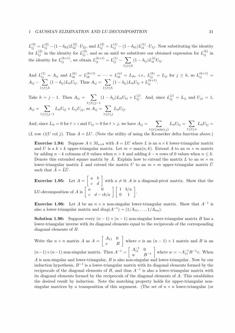
1 GAUSSIAN ELIMINATION AND LU-DECOMPOSITION 31
L(3)ij = L
(2)ij − (1− δh2)L
(2)i2 ·U2j , and L
(2)ij = L
(1)ij − (1− δh1)L
(1)i1 ·U1j . Now substituting the identity
for L(2)ij in the identity for L
(3)ij , and so on until we substitute our obtained expression for L
(h)ij in
the identity for L(h+1)ij , we obtain L
(h+1)ij = L
(1)ij −
∑
1≤t≤h
(1− δtj)L(t)it Utj .
And L(1)ij = Aij and L
(h)ih = L
(h+1)ih = · · · = L
(n)ih = Lih, i.e., L
(h)ij = Lij for j ≥ h, so L
(h+1)ij =
Aij −∑
1≤t≤h
(1− δtj)LitUtj . Thus Aij =∑
1≤t≤h
(1− δtj)LitUtj + L(h+1)ij .
Take h = j − 1. Then Aij =∑
1≤t≤j−1
(1 − δtj)LitUtj + L(j)ij . And, since L
(j)ij = Lij and Ujj = 1,
Aij =∑
1≤t≤j−1
LitUtj + LijUjj , so Aij =∑
1≤t≤j
LitUtj .
And, since Lit = 0 for t > i and Utj = 0 for t > j, we have Aij =∑
1≤t≤min(i,j)
LitUtj =∑
1≤t≤n
LitUtj =
(L row i)(U col j). Thus A = LU . (Note the utility of using the Kronecker delta function above.)
Exercise 1.94: Suppose A ∈Mn×k with A = LU where L is an n× k lower-triangular matrixand U is a k × k upper-triangular matrix. Let m = max(n, k). Extend A to an m×m matrixby adding n− k columns of 0 values when n > k and adding k−n rows of 0 values when n ≤ k.Denote this extended square matrix by A. Explain how to extend the matrix L to an m ×mlower-triangular matrix L and extend the matrix U to an m × m upper-triangular matrix Usuch that A = LU .
Exercise 1.95: Let A =
[
a bc d
]
with a 6= 0; A is a diagonal-pivot matrix. Show that the
LU-decomposition of A is
[
a 0c d− cb/a
] [
1 b/a0 1
]
.
Exercise 1.96: Let A be an n × n non-singular lower-triangular matrix. Show that A−1 isalso a lower-triangular matrix and diag(A−1) = (1/A11, . . . , 1/Ann).
Solution 1.96: Suppose every (n− 1)× (n− 1) non-singular lower-triangular matrix B has alower-triangular inverse with its diagonal elements equal to the reciprocals of the correspondingdiagonal elements of B.
Write the n × n matrix A as A =
[
A11 0v B
]
where v is an (n − 1) × 1 matrix and B is an
(n−1)×(n−1) non-singular matrix. Then A−1 =
[
A−111 0
w B−1
]
where w = −A−111 B−1v. When
A is non-singular and lower-triangular, B is also non-singular and lower-triangular. Now by ourinduction hypothesis, B−1 is a lower-triangular matrix with its diagonal elements formed by thereciprocals of the diagonal elements of B, and thus A−1 is also a lower-triangular matrix withits diagonal elements formed by the reciprocals of the diagonal elements of A. This establishesthe desired result by induction. Note the matching property holds for upper-triangular non-singular matrices by a transposition of this argument. (The set of n × n lower-triangular (or
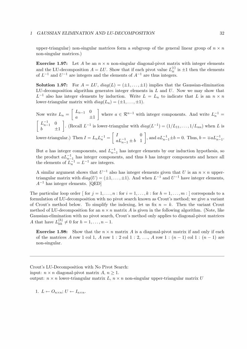
1 GAUSSIAN ELIMINATION AND LU-DECOMPOSITION 32
upper-triangular) non-singular matrices form a subgroup of the general linear group of n × nnon-singular matrices.)
Exercise 1.97: Let A be an n × n non-singular diagonal-pivot matrix with integer elements
and the LU-decomposition A = LU . Show that if each pivot value L(i)ii is ±1 then the elements
of L−1 and U−1 are integers and the elements of A−1 are thus integers.
Solution 1.97: For A = LU , diag(L) = (±1, . . . ,±1) implies that the Gaussian-eliminationLU-decomposition algorithm generates integer elements in L and U . Now we may show thatL−1 also has integer elements by induction. Write L = Ln to indicate that L is an n × nlower-triangular matrix with diag(Ln) = (±1, . . . ,±1).
Now write Ln =
[
Ln−1 0a ±1
]
where a ∈ Rn−1 with integer components. And write L−1n =
[
L−1n−1 0
b ±1
]
. (Recall L−1 is lower-triangular with diag(L−1) = (1/L11, . . . , 1/Lnn) when L is
lower-triangular.) Then I = LnL−1n =
[
I 0
aL−1n−1 ± b 1
]
, and aL−1n−1±b = 0. Thus, b = ∓aL−1
n−1.
But a has integer components, and L−1n−1 has integer elements by our induction hypothesis, so
the product aL−1n−1 has integer components, and thus b has integer components and hence all
the elements of L−1n = L−1 are integers.
A similar argument shows that U−1 also has integer elements given that U is an n × n upper-triangular matrix with diag(U) = (±1, . . . ,±1). And when L−1 and U−1 have integer elements,A−1 has integer elements. [QED]
The particular loop order [ for j = 1, . . . , n : for i = 1, . . . , k : for h = 1, . . . , m : ] corresponds to aformulation of LU-decomposition with no pivot search known as Crout’s method; we give a variantof Crout’s method below. To simplify the indexing, let us fix n = k. Then the variant Croutmethod of LU-decomposition for an n×n matrix A is given in the following algorithm. (Note, likeGaussian-elimination with no pivot search, Crout’s method only applies to diagonal-pivot matrices
A that have L(h)hh 6= 0 for h = 1, . . . , n− 1.
Exercise 1.98: Show that the n × n matrix A is a diagonal-pivot matrix if and only if eachof the matrices A row 1 col 1, A row 1 : 2 col 1 : 2, . . ., A row 1 : (n − 1) col 1 : (n − 1) arenon-singular.
Crout’s LU-Decomposition with No Pivot Search:input: n× n diagonal-pivot matrix A, n ≥ 1.output: n× n lower-triangular matrix L, n× n non-singular upper-triangular matrix U
1. L← On×n; U ← In×n.
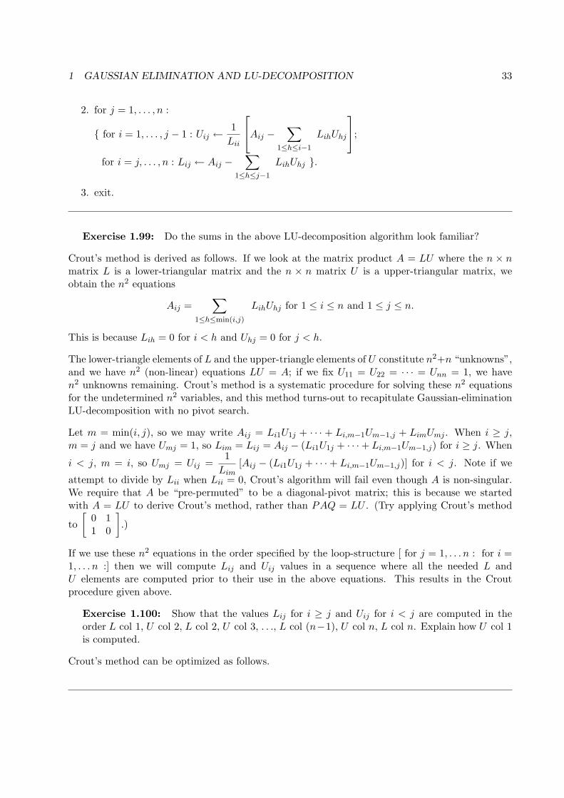
1 GAUSSIAN ELIMINATION AND LU-DECOMPOSITION 33
2. for j = 1, . . . , n :
{ for i = 1, . . . , j − 1 : Uij ←1
Lii
Aij −∑
1≤h≤i−1
LihUhj
;
for i = j, . . . , n : Lij ← Aij −∑
1≤h≤j−1
LihUhj }.
3. exit.
Exercise 1.99: Do the sums in the above LU-decomposition algorithm look familiar?
Crout’s method is derived as follows. If we look at the matrix product A = LU where the n × nmatrix L is a lower-triangular matrix and the n × n matrix U is a upper-triangular matrix, weobtain the n2 equations
Aij =∑
1≤h≤min(i,j)
LihUhj for 1 ≤ i ≤ n and 1 ≤ j ≤ n.
This is because Lih = 0 for i < h and Uhj = 0 for j < h.
The lower-triangle elements of L and the upper-triangle elements of U constitute n2+n “unknowns”,and we have n2 (non-linear) equations LU = A; if we fix U11 = U22 = · · · = Unn = 1, we haven2 unknowns remaining. Crout’s method is a systematic procedure for solving these n2 equationsfor the undetermined n2 variables, and this method turns-out to recapitulate Gaussian-eliminationLU-decomposition with no pivot search.
Let m = min(i, j), so we may write Aij = Li1U1j + · · · + Li,m−1Um−1,j + LimUmj . When i ≥ j,m = j and we have Umj = 1, so Lim = Lij = Aij − (Li1U1j + · · ·+ Li,m−1Um−1,j) for i ≥ j. When
i < j, m = i, so Umj = Uij =1
Lim[Aij − (Li1U1j + · · ·+ Li,m−1Um−1,j)] for i < j. Note if we
attempt to divide by Lii when Lii = 0, Crout’s algorithm will fail even though A is non-singular.We require that A be “pre-permuted” to be a diagonal-pivot matrix; this is because we startedwith A = LU to derive Crout’s method, rather than PAQ = LU . (Try applying Crout’s method
to
[
0 11 0
]
.)
If we use these n2 equations in the order specified by the loop-structure [ for j = 1, . . . n : for i =1, . . . n :] then we will compute Lij and Uij values in a sequence where all the needed L andU elements are computed prior to their use in the above equations. This results in the Croutprocedure given above.
Exercise 1.100: Show that the values Lij for i ≥ j and Uij for i < j are computed in theorder L col 1, U col 2, L col 2, U col 3, . . ., L col (n−1), U col n, L col n. Explain how U col 1is computed.
Crout’s method can be optimized as follows.
1 GAUSSIAN ELIMINATION AND LU-DECOMPOSITION 34
Crout’s LU-Decomposition with No Pivot Search:input: n× n diagonal-pivot matrix A, n ≥ 1.output: n× n lower-triangular matrix L, n× n upper-triangular matrix U , if successful.
1. L← On×n; U ← In×n.
2. for j = 1, . . . , n :for i = 1, . . . , n :{m← min(i, j); s← Aij ; for h = 1, . . . , m− 1 : s← s− LihUhj ;
if i ≥ j then Lij ← s else { if Lii = 0 then exit(“0 pivot encountered”);Uij ← s/Lii }}.
3. exit.
Note this procedure shows the flop-count similarity with matrix multiplication: we compute an(abbreviated) inner-product of L row i with U col j for 1 ≤ i ≤ n and 1 ≤ j ≤ n, resulting inO(n3) floating-point operations.
Exercise 1.101: Show that the “optimized” Crout procedure above uses 23n3 + 3
2n2 − 16n
floating-point operations, which is 2n2 more flops than our direct Gaussian-elimination LU-decomposition algorithm. Hint: sum the elements of the n × n matrix M defined by Mij =min(i, j). Can you account for the extra 2n2 flops?
Exercise 1.102: Let A be an n×n orthogonal lower-triangular matrix so that A−1 = AT andAij = 0 for i < j. Show that A = I.
For j = 1, . . . , n, Crout’s algorithm computes the n undetermined variables, first in U col j and thenin L col j, (excluding the “pre-determined” variables Ujj .) A version of Crout’s method includingcross-row partial-pivoting and scaling is given in [PTVF92]. We shall give a similar version below.The addition of cross-row partial-pivoting makes Crout’s method a viable procedure for comput-ing the LU-decomposition of a non-singular matrix, generally without excessive contamination byround-off error.
Exercise 1.103: Show that we can modify Crout’s procedure given above to overwrite thematrix A with the lower-triangle of L and the upper-triangle of U , less the main-diagonal ofU . Also propose a more efficient way to achieve diag(U) = (1, 1, . . . , 1) than the assignment“U ← In×n”.
Exercise 1.104: Show that, for any n×n matrix A, the Gaussian-elimination LU-decompositionalgorithm with no pivot search is equivalent to Crout’s LU-decomposition algorithm, i.e., exactlythe same termination state occurs and the same output L and U matrices are computed.
We give a version of Crout’s LU-decomposition algorithm with cross-row partial-pivoting below.The input is an n×n non-singular matrix A. The output is an n×n matrix B whose lower-triangledefines a non-singular lower-triangular matrix L, and whose strict upper-triangle defines a non-singular upper-triangular matrix U with diag(U) understood to be (1, 1, . . . , 1). The output vector
1 GAUSSIAN ELIMINATION AND LU-DECOMPOSITION 35
b is a transposition vector defining the n× n row-permutation matrix P = I row perm(b)−1. Theobtained LU-decomposition of A is PA = LU .
Crout’s LU-Decomposition with Cross-Row Partial-Pivoting:input: n× n non-singular matrix A, n ≥ 1.output: n × n matrix B holding the lower-triangle of the n × n lower-triangular matrix L andthe strict upper-triangle of the n× n upper-triangular matrix U , and the n-transposition vector bcorresponding to the permutation matrix P such that PA = LU , if successful.
1. define L = B; define U = B.
2. B ← A.
3. for j = 1, . . . , n :{for i = 1, . . . , n :{m← min(i, j); s← Bij ; for h = 1, . . . , m− 1 : s← s− LihUhj ;if i ≥ j then {Lij ← s; if i = j or s > v then {v ← s; x← i }}else Uij ← s};
if v = 0 then exit(“A is singular”);bj ← x; if j 6= x then swap B row j and B row x;
for i = j + 1, . . . , n : Uij ← Uij/v}.
4. exit.
Exercise 1.105: Explain why the above algorithm works as claimed.
Exercise 1.106: Let A be an n×n matrix and define A[i] := A row 1 : i col 1 : i; A[i] is calledthe i-th principal submatrix of A. Take A[0] = [1]. Suppose that A has an LU-decompositioncomputable with no pivot search, so A = LU and Lii 6= 0 for i = 1, . . . , n − 1. Show thatLii = det(A[i])/det(A[i−1]). (This implies that the diagonal-pivot matrix A has a direct LU-decomposition if and only if det(A[j]) 6= 0 for j = 0, 1, . . . , n− 1.)
Solution 1.106: We have A = LU where diag(U) = (1, . . . , 1) and Lii 6= 0 for 1 ≤ i ≤ n, so
A =
[
A[i] ∼∼ ∼
]
=
[
L[i] 0
∼ ∼
] [
U[i] ∼0 ∼
]
=
[
L[i]U[i] ∼∼ ∼
]
where each occurrence of the symbol ‘∼’ denotes a submatrix of the appropriate size thatconforms to all the implicit constraints on its value dictated by where it appears. This means
A[i] = L[i]U[i] for 1 ≤ i ≤ n. Thus A[i] =
[
L[i−1] 0
∼ Lii
] [
U[i−1] ∼0 1
]
for 2 ≤ i ≤ n.
1 GAUSSIAN ELIMINATION AND LU-DECOMPOSITION 36
Recall we have the determinant identity det(
[
X 0∼ Y
]
) = det(X)det((Y ). Therefore det(A[i]) =
det(L[i])det(U[i]) =[
det(L[i−1]) · Lii
] [
det(U[i−1]) · 1]
= det(A[i−1]) · Lii for 2 ≤ i ≤ n. Anddet(A[1]) = A11 = L11 so det(A[i]) = L11·L22 · · ·Lii for 1 ≤ i ≤ n. Thus Lii = det(A[i])/det(A[i−1]
where det(A[0]) = 1.
This formula for the pivot values we obtain with no pivot search serves as a test that determineswhether or not an n×n matrix A is a diagonal-pivot matrix. We compute det(A[1]), det(A[2]), . . .,det(A[n−1]); if all these determinant values are non-zero, A is a diagonal-pivot matrix, otherwiseA is not a diagonal-pivot matrix.
Exercise 1.107: Let Vn be the n×n Vandermonde matrix
1 x1 x21 . . . xn−1
1
1 x2 x22 . . . xn−1
2...
......
1 xn x2n . . . xn−1
n
. Show
that when x1, . . . , xn are distinct values, Vn is a diagonal-pivot matrix.
Exercise 1.108: Recall that we showed earlier that for x1, . . . , xn distinct, the Vandermondematrix Vn has the unique LU-decomposition Vn = LU where Lij = πj(xi) for 1 ≤ i ≤ n and1 ≤ j ≤ n where πj(x) is the Newton polynomial (x− x1)(x− x2) · · · (x− xj−1) with π1(x) = 1and πj(xi) = 0 for 1 ≤ i < j ≤ n, and Uij = hj−i(x1, . . . , xi) for 1 ≤ i ≤ n and 1 ≤ j ≤ nwhere, for i ≥ 0 and k ≥ 0, hi(x1, . . . , xk) is the complete symmetric function hi(x1, . . . , xk) =
∑
j1+j2+···+jk=ij1≥0,...,jk≥0
xj11 xj2
2 · · ·xjk
k . Note h0(x1, . . . , xk) = 1, and we define hi(x1, . . . , xk) = 0 for i < 0.
Is using this pre-established LU-decomposition always a good way to solve the linear equationscVn = y where y is a given n-vector and c ∈ Rn is the vector of coefficients of the interpolatingpolynomial for (x1, y1), . . . , (xn, yn) to be determined? Hint: Is the round-off error introducedwhile computing and using the elements of L and U in the course of back-substitution worsethan the error introduced in computing the LU-decomposition of Vn using cross-row partial-pivoting? Note using cross-row partial pivoting is roughly equivalent to ordering x1, . . . , xn indecreasing order. Can you find efficient error-reducing ways to compute hj−i(x1, . . . , xi) andπj(xi) for 1 ≤ i ≤ n?
Let A be an n × k rank r matrix with a direct LU-decomposition of the form A = LU (where nopermutations are involved.) Recall rank(A) = r implies the submatrix L row (r+1) : n col (r+1) :k = 0. Let m = min(n, k). The matrix A is an extended diagonal-pivot matrix in the sense that theLU-decomposition A = LU can be computed with no pivot search, terminating when a 0 pivot valueis encountered. An extension of the exercise above shows that the extended diagonal-pivot matrixA has the characterization that the principal submatrices A[0], A[1], . . ., A[r] are all non-singular,and A[r+1], . . ., A[m] are all singular.
Exercise 1.109: Let A be an n × k rank r matrix with A[r] = A row 1 : r col 1 : r non-singular. Let n = min(n, k). Show that det(A row (1 : h) col (1 : h)) = 0 for r < h ≤ m. Hint:the rows of A row (r + 1) : n are all linear combinations of the vectors A row 1, . . ., A row r.
The LU-decomposition of the n× k rank r extended diagonal-pivot matrix A is determined by the
1 GAUSSIAN ELIMINATION AND LU-DECOMPOSITION 37
LU-decomposition of the r×r non-singular diagonal-pivot matrix A row 1 : r col 1 : r = A[r] =: A11.(Note that in this discussion only, Lij , Uij , and Aij denote submatrices, not elements, of the matricesL, U , and A.)
Write
[
A11 A12
A21 A22
]
=
[
L11 0L21 L22
] [
U11 U12
0 U22
]
=
[
L11U11 L11U12
L21U11 L21U12 + L22U22
]
where L11,
U11, and U22 are non-singular triangular matrices.
Then L21 = A21U−111 , U12 = L−1
11 A12, and L22 and U22 satisfy L22U22 = 0 so we may choose L22 = 0and U22 = Ik−r,k−r. We have L22U22 = 0 because A is a rank r extended diagonal-pivot matrix andhence there is an (n− r)× r matrix B such that B [A11 A12] = [A21 A22] (i.e., (B row j) [A11 A12]is a linear combination of the rows of [A11 A12],) so BA11 = A21 and BA12 = A22 and
A22 = L21U12 + L22U22
= A21U−111 L−1
11 A12 + L22U22
= BA11U−111 L−1
11 A12 + L22U22
= BA11A−111 A12 + L22U22
= BA12 + L22U22
= A22 + L22U22
and thus L22U22 = 0. Thus the extended diagonal-pivot matrix A has an LU-decomposition com-putable with no pivot search, i.e., once L11 and U11 are determined, the entire LU-decompositionof A is determined.
We can now see that the effect of the permutation matrices P and Q produced in our Gausssian-elimination LU-decomposition algorithm is to permute the columns and the rows of the n×k matrixA so that the principal submatrices (PAQ)[i] are all non-singular for i = 1, . . . , rank(A), and theremaining principal submatrices (PAQ)[i] for i = rank(A) + 1, . . . ,min(n, k) are all singular, i.e.,PAQ is an extended diagonal-pivot matrix.
Although any extended diagonal-pivot matrix has a direct LU-decomposition, not all matrices withdirect LU-decompositions are extended diagonal-pivot matrices when we relax the forms of thefactors L and U to merely be lower-triangular and upper-triangular matrices respectively withoutfurther structural conditions. Of course such a relaxed LU-decomposition is less useful than thestrict form we focus on herein. Such relaxed direct LU-decompositions arise when either the firstr rows or the first r columns of a rank r matrix are not linearly-independent.
Exercise 1.110: Show that
[
0 01 2
]
=
[
0 01 1
] [
1 10 1
]
=
[
0 01 0
] [
1 20 0
]
.
Pavel Okunev and Charles Johnson [OJ97] show that an n × n matrix A has a direct (relaxed)LU-decomposition A = LU if and only if rank(A[h]) + h ≥ rank(A row 1 : h col 1 : n) +rank(A row 1 : n col 1 : h) for h = 1, . . . , n. They also give the following algorithm to computesuch a direct LU-decomposition.
1 GAUSSIAN ELIMINATION AND LU-DECOMPOSITION 38
Okunev and Johnson’s Relaxed LU-Decomposition with No Pivot Search:input: n× n Okunev matrix A, n ≥ 1.output: n× n lower-triangular matrix L, n× n upper-triangular matrix U , if successful.
1. L← On×n; U ← On×n.
2. for h = 1, . . . , n :[for i = 1, . . . , n :[for j = i, . . . , n :
[if Aij 6= 0 then {L col h← A col j; U row h← (A row i)/Aij ; goto α};if Aji 6= 0 then {L col h← A col i; U row h← (A row j)/Aji; goto α};]
]
α: A← A− (L col h)(U row h).]
3. exit.
Exercise 1.111: Explain why the above algorithm works. (Recall for n × n matrices A and
B, the product C = AB satisfies C =∑
1≤h≤n
(A col h)(B row h).)
Froilan Dopico, Charles Johnson and Juan Molera [DJM06] have given a characterization of thosen × n matrices that have multiple semi-relaxed LU-decompositions with diag(L) = (1, . . . , 1) (orequivalently, with diag(U) = (1, . . . , 1),) and shown how to generate all these LU-decompositionsin terms of the elements of L (or equivalently, U .)
Exercise 1.112: Show that
[
0 01 1
]
has an infinite number of semi-relaxed LU-decompositions.
Solution 1.112:
[
0 01 1
]
=
[
0 01 1− a
] [
1 a0 1
]
for a ∈ R. How many semi-relaxed LU-
decompositions does
[
0 10 1
]
possess? (Note
[
0 10 1
]
=
[
1a 00 1
] [
0 a0 1
]
for a ∈ R− {0}.)
Exercise 1.113: Let LTn×n be the subset of all n× n non-singular lower-triangular matricesin the set GLn×n(Rn). Show that LTn×n is a normal subgroup of the group GLn×n(Rn) of alln × n non-singular matrices on Rn. Hint: use the QR-decomposition of an n × n non-singularmatrix AT to show that for any L ∈ LTn×n there exists L ∈ LTn×n such that AL = LA, andalso show that for A ∈ GLn×n(Rn) and L1, L2 ∈ LTn×n, AL1 = AL2 implies L1 = L2. Can youfind some subgroups of LTn×n?
Exercise 1.114: What is the dimension of LTn×n?
1 GAUSSIAN ELIMINATION AND LU-DECOMPOSITION 39
Solution 1.114: The set of all n × n lower-triangular matrices is an algebra of dimensionn(n + 1)/2, and hence dim(LTn×n) = n(n + 1)/2. Note the set of all n × n strictly lower-triangular matrices with diagonal (0, . . . , 0) is an algebra of dimension (n − 1)n/2 with theinteresting property that Ln = On×n for every member L.
When an n × n matrix A is a non-singular diagonal-pivot matrix, it has an LU-decompositionA = LU , computable by the Gaussian-elimination LU-decomposition algorithm with no pivotsearch, and all the diagonal elements of the lower-triangular matrix L that serve as the successivepivot values are non-zero. This means we can “factor” the matrix L into a matrix product LDwhere D is the diagonal matrix diag(L11, . . . , Lnn) and L is the non-singular lower-triangular matrixspecified by L col i = (L col i)/Lii for i = 1, . . . , n; this results in diag(L) = (1, . . . , 1). In thissituation, we have A = LDU , or relabeling to reuse the symbol L to denote L, we have A = LDUwhere diag(L) and diag(U) are both (1, 1, . . . , 1) and D is a diagonal matrix.
Exercise 1.115: Let A be an n × n rank r extended diagonal-pivot matrix with the LU-decomposition A = LU . Show that A can be written as LDU where L is a lower-triangularmatrix with diag(L) = (1, . . . , 1) and D = diag(L11, . . . , Lr,r, 0, . . . , 0).
Now if A is a symmetric matrix as well as a non-singular diagonal-pivot matrix, then we can writeA = LDLT where L is a lower-triangular matrix with diag(L) = (1, . . . , 1) and D is a diagonalmatrix with non-zero diagonal elements. We may derive this decomposition from the decompositionA = LDU .
When A is a symmetric non-singular diagonal-pivot matrix with A = LDU as described above,we have (UT)−1AU−1 = (UT)−1LD. And [(UT)−1AU−1]T = (UT)−1AU−1 so (UT)−1AU−1 issymmetric. But (UT)−1LD is the product of lower-triangular matrices so (UT)−1LD is itselflower-triangular as well as symmetric. This means (UT)−1LD is is a diagonal matrix. But then(UT)−1L is diagonal since D is diagonal.
We also have diag((UT)−1) = (1, . . . , 1) and diag(L) = (1, . . . , 1) so (UT)−1L = I. ThereforeL = UT and hence A = LDLT when A is a symmetric non-singular diagonal-pivot matrix. [QED]
Exercise 1.116: Given the quadratic form xAxT where A is an n×n symmetric non-singularmatrix with A = LDLT where L is a lower-triangular matrix with diag(L) = (1, . . . , 1) andD = diag(d1, . . . , dn) with di ∈ R for 1 ≤ i ≤ n, show that the transformation x → xLtransforms the quadratic form xAxT into the diagonal quadratic form xDxT.
Now when A is a symmetric non-singular diagonal-pivot matrix with A = LDLT where L is alower-triangular matrix with diag(L) = (1, . . . , 1) and D is a diagonal matrix with Dii > 0 for
i = 1, 2, . . . , n, then we can define D1
2 = diag(√
D11, . . . ,√
Dnn) and write A = LD1
2 D1
2 LT. (Weshall call a symmetric non-singular diagonal-pivot matrix where each pivot value is positive apositive-definite matrix.)
But LD1
2 D1
2 LT = LD1
2 (D1
2 )TLT = GGT where G = LD1
2 . The decomposition A = GGT where Gis a lower-triangular matrix is called the Cholesky decomposition of A. Since the LU-decompositionof a non-singular matrix is unique, the Cholesky decomposition of a positive-definite matrix isunique. (Note if we admit complex elements, any symmetric non-singular matrix has a Choleskydecomposition.)
1 GAUSSIAN ELIMINATION AND LU-DECOMPOSITION 40
When A is a positive-definite matrix (i.e., a symmetric non-singular positive diagonal-pivot matrix,)with an LDLT decomposition where Dii > 0 for i = 1, 2, . . . , n, the Cholesky decomposition of Acan be computed with the following algorithm.
Cholesky-Decomposition:input: n× n symmetric non-singular positive-definite matrix A, n ≥ 1.output: n× n lower-triangular matrix G such that A = GGT
1. G← On×n.
2. for j = 1, . . . , n :
{Gjj ←
Ajj −∑
1≤t<j
A2jt
1
2
; for i = 1, . . . , n : Gij ←1
Gjj
Aij −∑
1≤t<j
AitAjt
}.
3. exit.
Exercise 1.117: Explain why the above algorithm is correct. Hint: derive the equations fromA = GGT in the way Crout’s method was obtained or see [GV89].
Exercise 1.118: Explain how to use the Cholesky decomposition of a symmetric non-singularpositive diagonal-pivot matrix A to solve the equations xA = v.
Exercise 1.119: Compute the number of flops needed to compute the n×n Cholesky matrixG in the above algorithm assuming that computing a square-root is s times more costly than afloating-point multiply.
We should include a test in the above algorithm to ensure that round-off error does not result intrying to compute the square-root of a negative number, although for a well-conditioned matrix,this is unlikely. We should also guard against dividing by a too-small value as we discussed withrespect to the Gaussian-elimination LU-decomposition algorithm. Golub and Van Loan [GV89]discuss the “failure modes” of the above algorithm and discuss the error in G that is expected tobe introduced in terms of the elements of the input matrix A.
Note the QR-decomposition and the Cholesky decomposition are related. Let A be an n×n matrixwith the QR-decomposition A = QR where Q is an n × n orthogonal matrix and R is an n × nupper-triangular matrix. Then ATA = RTQTQR = RTR; this is a form of LU-decompositionof ATA as well as a generalized Cholesky decomposition. When A is non-singular, the Choleskydecomposition of ATA is unique and RTR is that Cholesky decomposition.
Exercise 1.120: Let A be an n × n non-singular matrix. Show how to use the Choleskydecomposition of the n× n matrix ATA to compute the QR-factorization of A.
1 GAUSSIAN ELIMINATION AND LU-DECOMPOSITION 41
Exercise 1.121: Given the n × k rank r matrix A, suppose we have the LU-decompositionPAQ = LU . Describe how we can easily obtain the decomposition A = FGT where F is an n×rrank r matrix with linearly-independent columns, and G is a k× r rank r matrix with linearly-independent columns. (Recall that this decomposition is the starting point for constructing theMoore-Penrose pseudo-inverse matrix A+.)
Exercise 1.122: Show how to use the LU-decomposition PAQ = LU of the n × k matrix Atogether with four back-substitution steps to solve the normal equations xAAT = bAT whereb ∈ Rk and x ∈ Rn. How much does this cost in comparison to computing B = AAT and thensolving xB = bAT by computing an LU-decomposition of B? Note AAT is symmetric, so Bcan be computed at less cost than just multiplying A by AT. When can we employ a Choleskydecomposition to solve the normal equations xAAT = bAT? (Recall that a vector x that satisfiesxAAT = bAT minimizes |xA− b|, and x = bA+ is such a vector with least norm.)
Exercise 1.123: Suppose A is an n × n non-singular matrix. Explain how to use the LU-decomposition PAQ = LU to compute A−1. Hint: look at A−1A = I as n sets of linearequations: xA = e1, . . . , xA = en.
Exercise 1.124: Explain how to use the LU-decomposition of the n×n non-singular matrix Ato efficiently compute the matrix product BA−1 where B is a given k×n matrix. Hint: considersolving xiA = B row i for i = 1, . . . , k.
We stated above that when the n×n matrix A is non-singular, use of cross-column partial-pivotingensures that we can write AC1M1 · · ·CrMr = L, where L is an n×n non-singular lower-triangularmatrix (so that Lii 6= 0 for 1 ≤ i ≤ n.)
By multiplying at most v := n(n + 1)/2 particular non-singular elementary matrices on the rightof L, the non-singular matrix L can be reduced to the n × n identity matrix. These elementarymatrices H1, . . . , Hv are chosen to effect the same transformations as achieved by the followingprogram: [for i = n, n− 1, . . . , 2 : (for j = 1, 2 . . . , i− 1 : (Lij ← Lij − (Lij/Lii)Lii));for i = 1, 2 . . . , n : (Lii ← Lii/Lii)].
Exercise 1.125: Let 1 ≤ j < i ≤ n. Show that the elementrary matrix that zeros Lij
is En[i, j,−Lij/Lii]. Then show that for 1 ≤ k ≤ n(n − 1)/2, the elementary matrix Hk isEn[i, j,−Lij/Lii] where i = p+1 and j = s−i(i−1)/2 with s = 1+n(n−1)/2−k and p = ⌊
√2s⌋.
(Also, for n(n− 1)/2 + 1 ≤ k ≤ n(n + 1)/2, Hk = En[r, r, L−1rr − 1] where r = k − n(n− 1)/2.)
Thus AC1M1 · · ·CrMrH1 · · ·Hv = I, so A−1 = C1M1 · · ·CrMrH1 · · ·Hv andA = H−1
v · · ·H−11 C−1
r H−1v M−1
r C−1r · · ·M−1
1 C−11 . Note that H−1
1 , . . . , H−1v , M−1
1 , . . . , M−1r , and
C−11 , . . ., C−1
r are all elementary matrices or products of elementary matrices; thus A is written asa product of elementary matrices. (What is the minimum number of n × n elementary matricesthat must be multiplied to guarantee that any non-singular n× n matrix can be produced?)
Exercise 1.126: Let A be an n×n non-singular matrix. Show that application of the algorithmbelow to the matrix A exits at step 7 and that, at exit, B is indeed A−1.
1. h← 1; B ← In×n.
2. a← 0; for i = h, . . . , n : if (Ahi 6= 0) then {a← Ahi; q ← i; goto step 3}.
1 GAUSSIAN ELIMINATION AND LU-DECOMPOSITION 42
3. if a = 0 then exit(“A is singular.”).
4. if (q 6= h) then {swap A col h and A col q in A; swap B row h and B row q in B; }.5. A col h← (A col h)/a; B col h← (B col h)/a.
6. for i = 1, . . . , n :if (i 6= h) then {A col i← (A col i)−Ahi(A col i); B col i← (B col i)−Ahi(B col i)}.
7. if h = n then exit(“B = A−1.”).
8. h← h + 1; go to step 2.
Exercise 1.127: Can any n × n matrix, not necessarily non-singular, be represented by aproduct of elementary matrices, as defined here?
Exercise 1.128: Let A be an n× n symmetric matrix. Show that there exists a non-singularmatrix F such that FAFT is a diagonal matrix of the form diag(1, . . . , 1,−1, . . . ,−1, 0, . . . , 0)where there are s1 ones, followed by s2 minus-ones, followed by s3 zeros, with s1 ≥ 0, s2 ≥ 0,s3 ≥ 0, and s1 + s2 + s3 = n. Hint: Let B denote the matrix C1M1 · · ·CrMr in the identityAC1M1 · · ·CrMr = L expressing the reduction of A to lower-triangular form via cross-columnpartial-pivoting. Now express B as a product of elementary matrices Ek · · ·E2E1. Then defineFT = BST
1 · · ·STn where Si = En[i, i, |Lii|1/2 − 1]. The values s1, s2 and s3, are symmetric-
congruence invariants; that is, if A and X are congruent n × n symmetric matrices, then(s1, s2, s3) for A is the same as (s1, s2, s3) for X.
Exercise 1.129: Give a recursive version of the Gaussian-elimination LU-decomposition algo-rithm where the LU-decomposition PTLUQT of an n×k matrix A is computed from the similarLU-decomposition of the (n− 1)× (k − 1) matrix A row 2 : n col 2 : k.
Neither Gaussian elimination with complete-pivoting nor Gaussian elimination with partial-pivotingtogether with back-substitution are guaranteed effective algorithms per se since the relative errorintroduced in the solution vector x that is intended to satisfy xA = v can be arbitrarily large incertain “ill-conditioned” cases. (The error in a solution x to xA = v is measured by the quantity|x− x| and the relative error is |x− x|/|x| when |x| 6= 0.) It may be more appropriate to say thatGaussian elimination with complete-pivoting or partial-pivoting is effective for well-conditionedproblems.
The condition of an n× n system of linear equations xA = v is measured by the condition numberκ(A) of the coefficient matrix A. The condition number depends on the norm being used, but allnorms are comparable in a sense that we shall make precise below. The ∞-norm condition number
of the n × n matrix A is defined as κ∞(A) =
max1≤i≤n
∑
1≤j≤n
|Aij |
·
max≤i≤n
∑
1≤j≤n
|(A−1)ij |
when
A is non-singular and ∞ when A is singular; κ(A) essentially measures how close to singular thecoefficient matrix A is. The problem xA = v is ill-conditioned when κ(A) is large (what ‘large’means is dependent on the accuracy desired.)
One way to improve the condition of the matrix A, other than “damaging” A by adding to its di-agonal elements, is to replace A by AS and v by vS, where the k× k matrix S is a diagonal matrixthat scales the j-th equation x(A col j) = vj by the constant Sjj to obtain the equivalent equa-tion x(A col j)Sjj = vjSjj . Generally we want to choose the scaling factors S11, S22, . . . , Skk to
1 GAUSSIAN ELIMINATION AND LU-DECOMPOSITION 43
make each equation similar in “size”. For example, we could use Sjj = 1/|A col j|, or Sjj =1/ max1≤i≤n |Aij |. Note this scaling could be done, either explicitly or implicitly, within theGaussian-elimination LU-decomposition algorithm given above. If we choose the elements of thescale matrix S to be powers of 2, we will not directly introduce any additional round-off error inour LU-decomposition. We can obtain more flexiblity by scaling both rows and columns of A; givenscale matrices T and S, we can use the LU-decomposition of TAS to solve yTAS = vS for y andthen compute x = yT . Again, it is convenient to take the scale matrices T and S to be diagonalmatrices.
One reasonable way to define the scaling matrices T and S is as follows. Let ci denote an indexj such that |Aij | = maxm |Aim| and let rj denote an index i such that |Aij | = maxm |Amj |. Thenwe may define Tij = Sij = 0 for i 6= j and Tii = f(|Ai,ci
|−1/2) and Sjj = f(|Arj ,j |−1/2) wheref(x) = δx0 + x.
Note that using scaling subverts the notion of using an eligible element of maximum magnitude inthe current coefficient matrix as the pivot value in each iteration. However using large magnitudepivot values in early iterations might, in some circumstances, cause us to have to use excessivelysmall magnitude elements as the pivot values in later iterations; scaling may ameliorate this po-tential problem. It is difficult to know in advance when scaling will be beneficial, and, in that case,what scale factors should be used. An algorithm for computing scale factors has been proposed byOlschowka and Neumaier [ON96].
Note that scaling with diagonal scale matrices T and S can be “virtually” implemented withoutactually scaling any of the coefficients in the matrix A; this avoids introducing round-off error dueto scaling. All that such implicit scaling really does is change our choice of pivot elements whenusing a complete or partial or rook pivot search. (Although generally we only consider scaling whenwe are using a cross-row or cross-column pivot search.)
The fundamental computations in our Gaussian-elimination LU-decomposition algorithm are
Lij ← Lij −Lhj
LhhLih and Uhj ←
Lhj
Lhh.
When diagonal scaling matrices T and S are used, these computations become
Lij ← Tσi,σiLijSρj ,ρj
−Tσh,σh
LhjSρj ,ρj
Tσh,σhLhhSρh,ρh
Tσi,σiLihSρh,ρh
and Uhj ←Tσh,σh
LhjSρj ,ρj
Tσh,σhLhhSρh,ρh
,
where L row i holds the elements derived from A row σi and L col j holds the elements derivedfrom A col ρj during iteration h. Thus σ and ρ are permutation vectors that keep track of the rowand column exchanges done to bring the selected pivot element to the diagonal position Lhh atiteration h for h = 1, . . . , n.
These computations reduce to
Lij ← Tσi,σi
[
Lij −Lhj
LhhLih
]
Sρh,ρhand Uhj ←
LhjSρj ,ρj
LhhSρh,ρh
.
Thus Lij is computed as Tσi,σiSρj ,ρj
times the unscaled value that would normally be assignedto Lij , and Uhj is computed as (Sρh,ρh
)−1Sρj ,ρjtimes the unscaled value that would normally be
assigned to Uhj .
1 GAUSSIAN ELIMINATION AND LU-DECOMPOSITION 44
Since this computation of Lij holds in the initial iteration with L = A, it holds in every subsequentiteration as well. Thus we can dispense with multiplying Lij by Tσi,σi
Sρh,ρhand multiplying Uhj by
S−1ρh,ρh
Sρj ,ρjaltogether as long as we take into account this “virtual” implicit scaling when selecting
the pivot element that is permuted into Lhh in each iteration!
All we need do to employ implicit scaling with the diagonal scale matrices T and S is to initializethe permutation vector σ to 〈1, 2, . . . , n〉 and initialize the permutation vector ρ to 〈1, 2, . . . , k〉in step 1, and replace step 2 in our Gaussian-elimination LU-decomposition algorithm with thestatements
{Determine indices p ∈ {h, . . . , n} and q ∈ {h, . . . , k} such that |Lpq| = maxh≤i≤nh≤j≤k
|Tσi,σiLijSρj ,ρj
|;
Swap σp and σh; Swap ρq and ρh}.
This, in effect, chooses a sequence of pivot elements that sacrifices maximal magnitudes for lowervariation. (Note there is no reason to maintain both the permutations σ and ρ and also thetransposition vectors b and c in our LU-decomposition algorithm.)
We can justify this conclusion as follows. Let PAQ = LU be the LU-decomposition of the matrixA computed using the pivot elements determined by the pivot search procedure using the scalematrices T and S given above. We have P = I row σ and Q = I col ρ. Also let PTASQ = LsUs
be the LU-decomposition of the scaled matrix TAS computed with the ordinary complete-pivotingversion of our Gaussian-elimination LU-decomposition algorithm. Note the permutation matricesP and Q are the same in both decompositions.
For T and S non-singular diagonal matrices, we have effectively shown that Ls = TσLSρ andUs = S−1
ρ USρ where Tσ = diag(Tσ1,σ1, Tσ2,σ2
, . . ., Tσn,σn) = PTPT and Sρ = diag(Sρ1,ρ1, Sρ2,ρ2
,
. . ., Sρk,ρk) = QTSQ.
Thus PTASQ = LsUs = TσLSρS−1ρ USρ = PTPTLUQTSQ.
And then TAS = TPTLUQTS, so we may “unscale” by multiplying on the left by T−1 and on theright by S−1 to obtain A = PTLUQT, or equivalently, PAQ = LU .
Thus computing the LU-decomposition PAQ = LU with pivot values determined by implicitscaling is equivalent to computing the LU-decomposition PTASQ = LsUs and then “un-scaling”by computing (PT )−1LsUs(SQ)−1.
Exercise 1.130: Can you give a “dynamic” scaled pivot search where you strike a balancebetween partial-pivoting with scaling and complete-pivoting with no scaling by accepting thepivot element Lpq when Lpq is not too small, but making another choice when Lpq is too small?
Exercise 1.131: Since the average amount of computation for solving an (n + 1) × (n + 1)system of linear equations increases by O(2n2) operations from the cost of solving an n × nsystem of linear equations, is it the case that almost all “random” square systems of linearequations xA = v will exhibit unbounded relative error in x as n → ∞ when fixed finite-precision arithmetic is used?
1 GAUSSIAN ELIMINATION AND LU-DECOMPOSITION 45
Exercise 1.132: Let An be the n× n matrix defined by (An)ij = 1/(i + j − 1). This matrixis called a Hilbert matrix [Knu73]. Let vn = e1 + e2 + · · · + en. Write a program that uses anLU-decomposition to solve xAn = vn, both with complete-pivoting and with cross-row partial-pivoting, and with and without implicit scaling.
Compare your results for n = 2, 3, . . . , 9. Note you cannot represent a Hilbert matrix exactlyin floating-point format and this will cause some of the difficulties in computation that you willobserve. Why don’t all inexactly-represented matrices cause trouble?
Exercise 1.133: Another way to compute x ∈ Rn such that xA = v, where A is an n × nnon-singular matrix and v ∈ Rn, is to use the QR-factorization, or more precisely, its transpose,the LQT-factorization. We may write A = LQT where here L is an n×n lower-triangular rank nmatrix and Q is an n×n orthogonal matrix with Q−1 = QT. Then xLQT = v so xL = vQ, andthis is a triangular system of linear equations, and thus we can compute x via back-substitution.
In practice, the orthogonal matrix Q is computed as a product of Householder reflection matricesthat, when multiplying A on the right, produce a lower-triangular matrix. An alternate way ofcomputing L and QT essentially involves applying the Gram-Schmidt procedure to the rows ofA, keeping each intermediate inner-product and the final set of orthonormal vectors from whichwe form L and QT.
Explain why this method for solving xA = v is not cost-competitive with either direct Gaussianelimination or use of an LU-decomposition. Research when use of the QR-factorization approachto solving a set of linear equations is justified.
Exercise 1.134: There are a variety of other methods for solving systems of linear equationsbesides Gaussian elimination. (Look-up the Gauss-Seidel and conjugate gradient iterations.) Aniterative method that generates a sequence of approximate solution vectors x(0), x(1), . . . , x(s), . . .succeeds when this sequence converges to a solution x of the linear system xA = v. Assumingconvergence occurs with exact arithmetic, can such a method be guaranteed to yield a solutionwhose relative error is bounded as n→∞ when implemented in fixed finite-precision arithmetic?Hint: the convergence test itself must be done with the same fixed finite-precision arithmetic.
Exercise 1.135: Since the accuracy of the solution is sometimes poor, why is Gaussian elim-ination with complete-pivoting or partial-pivoting often used in practice?
A version of our LU-decomposition algorithm incorporating implicit scaling and using a test for azero pivot value involving an “approximation to zero” is given below
LU-Decomposition by Column-Operation Gaussian Elimination with Implicit Scaling and Complete-Pivoting:input: n× k matrix A, n ≥ 1, k ≥ 1.output: L, U overwritten in A, σ, ρ, r
1. Define L = A; Define U = A.
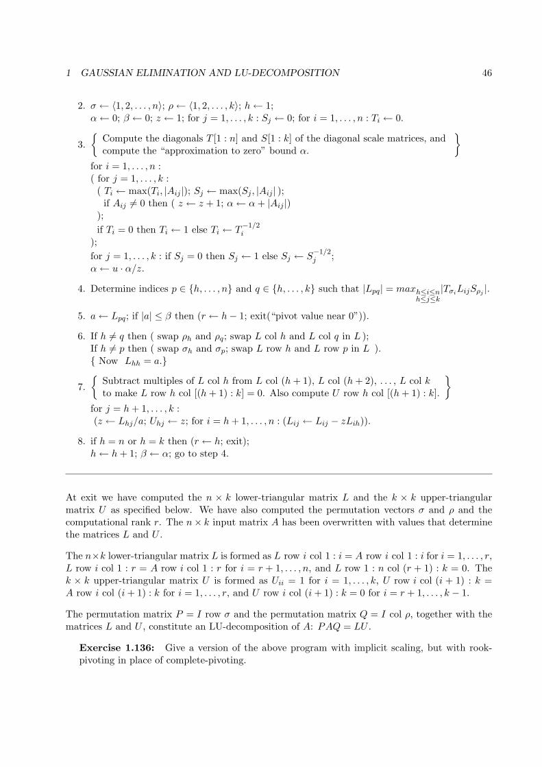
1 GAUSSIAN ELIMINATION AND LU-DECOMPOSITION 46
2. σ ← 〈1, 2, . . . , n〉; ρ← 〈1, 2, . . . , k〉; h← 1;α← 0; β ← 0; z ← 1; for j = 1, . . . , k : Sj ← 0; for i = 1, . . . , n : Ti ← 0.
3.
{
Compute the diagonals T [1 : n] and S[1 : k] of the diagonal scale matrices, andcompute the “approximation to zero” bound α.
}
for i = 1, . . . , n :( for j = 1, . . . , k :( Ti ← max(Ti, |Aij |); Sj ← max(Sj , |Aij | );if Aij 6= 0 then ( z ← z + 1; α← α + |Aij |)
);
if Ti = 0 then Ti ← 1 else Ti ← T−1/2i
);
for j = 1, . . . , k : if Sj = 0 then Sj ← 1 else Sj ← S−1/2j ;
α← u · α/z.
4. Determine indices p ∈ {h, . . . , n} and q ∈ {h, . . . , k} such that |Lpq| = maxh≤i≤nh≤j≤k
|TσiLijSρj
|.
5. a← Lpq; if |a| ≤ β then (r ← h− 1; exit(“pivot value near 0”)).
6. If h 6= q then ( swap ρh and ρq; swap L col h and L col q in L );If h 6= p then ( swap σh and σp; swap L row h and L row p in L ).{ Now Lhh = a.}
7.
{
Subtract multiples of L col h from L col (h + 1), L col (h + 2), . . . , L col kto make L row h col [(h + 1) : k] = 0. Also compute U row h col [(h + 1) : k].
}
for j = h + 1, . . . , k :(z ← Lhj/a; Uhj ← z; for i = h + 1, . . . , n : (Lij ← Lij − zLih)).
8. if h = n or h = k then (r ← h; exit);h← h + 1; β ← α; go to step 4.
At exit we have computed the n × k lower-triangular matrix L and the k × k upper-triangularmatrix U as specified below. We have also computed the permutation vectors σ and ρ and thecomputational rank r. The n× k input matrix A has been overwritten with values that determinethe matrices L and U .
The n×k lower-triangular matrix L is formed as L row i col 1 : i = A row i col 1 : i for i = 1, . . . , r,L row i col 1 : r = A row i col 1 : r for i = r + 1, . . . , n, and L row 1 : n col (r + 1) : k = 0. Thek × k upper-triangular matrix U is formed as Uii = 1 for i = 1, . . . , k, U row i col (i + 1) : k =A row i col (i + 1) : k for i = 1, . . . , r, and U row i col (i + 1) : k = 0 for i = r + 1, . . . , k − 1.
The permutation matrix P = I row σ and the permutation matrix Q = I col ρ, together with thematrices L and U , constitute an LU-decomposition of A: PAQ = LU .
Exercise 1.136: Give a version of the above program with implicit scaling, but with rook-pivoting in place of complete-pivoting.
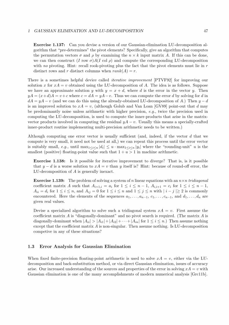
1 GAUSSIAN ELIMINATION AND LU-DECOMPOSITION 47
Exercise 1.137: Can you devise a version of our Gaussian-elimination LU-decomposition al-gorithm that “pre-determines” the pivot elements? Specifically, give an algorithm that computesthe permutation vectors σ and ρ by examining the n × k input matrix A. If this can be done,we can then construct (I row σ)A(I col ρ) and compute the corresponding LU-decompositionwith no pivoting. Hint: recall rook-pivoting plus the fact that the pivot elements must lie in rdistinct rows and r distinct columns when rank(A) = r.
There is a sometimes helpful device called iterative improvement [PTVF92] for improving oursolution x for xA = v obtained using the LU-decomposition of A. The idea is as follows. Supposewe have an approximate solution y with y = x + d, where d is the error in the vector y. ThenyA = (x+d)A = v+c where c = dA = yA−v. Thus we can compute the error d by solving for d indA = yA− v (and we can do this using the already-obtained LU-decomposition of A.) Then y − dis an improved solution to xA = v, (although Golub and Van Loan [GV89] point-out that d maybe predominantly noise unless arithmetic with higher precision, e.g., twice the precision used incomputing the LU-decomposition, is used to compute the inner-products that arise in the matrix-vector products involved in computing the residual yA− v. Usually this means a specially-craftedinner-product routine implementing multi-precision arithmetic needs to be written.)
Although computing one error vector is usually sufficient (and, indeed, if the vector d that wecompute is very small, it need not be used at all,) we can repeat this process until the error vectoris suitably small, e.g., until max1≤i≤n |di| ≤ u · max1≤i≤n |yi| where the “rounding-unit” u is thesmallest (positive) floating-point value such that 1 + u > 1 in machine arithmetic.
Exercise 1.138: Is it possible for iterative improvement to diverge? That is, is it possiblethat y − d is a worse solution to xA = v than y itself is? Hint: because of round-off error, theLU-decomposition of A is generally inexact.
Exercise 1.139: The problem of solving a system of n linear equations with an n×n tridiagonalcoefficient matrix A such that Ai+1,i = ai for 1 ≤ i ≤ n − 1, Ai,i+1 = ci for 1 ≤ i ≤ n − 1,Aii = di for 1 ≤ i ≤ n, and Aij = 0 for 1 ≤ i ≤ n and 1 ≤ j ≤ n with | i− j |≥ 2 is commonlyencountered. Here the elements of the sequences a1, . . . , an−1, c1, . . . , cn−1, and d1, . . . , dn aregiven real values.
Devise a specialized algorithm to solve such a tridiagonal system xA = v. First assume thecoefficient matrix A is “diagonally-dominant” and no pivot search is required. (The matrix A isdiagonally-dominant when |Aii| > |Ai1|+ |Ai2|+ · · ·+ |Ain| for 1 ≤ i ≤ n.) Then assume nothingexcept that the coefficient matrix A is non-singular. Then assume nothing. Is LU-decompositioncompetive in any of these situations?
1.3 Error Analysis for Gaussian Elimination
When fixed finite-precision floating-point arithmetic is used to solve xA = v, either via the LU-decomposition and back-substitution method, or via direct Gaussian elimination, issues of accuracyarise. Our increased understanding of the sources and properties of the error in solving xA = v withGaussian elimination is one of the many accomplishments of modern numerical analysis [Grc11b].
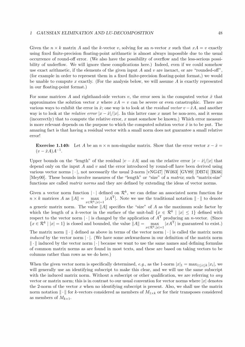
1 GAUSSIAN ELIMINATION AND LU-DECOMPOSITION 48
Given the n × k matrix A and the k-vector v, solving for an n-vector x such that xA = v exactlyusing fixed finite-precision floating-point arithmetic is almost always impossible due to the usualoccurrence of round-off error. (We also have the possibility of overflow and the less-serious possi-bility of underflow. We will ignore these complications here.) Indeed, even if we could somehowuse exact arithmetic, if the elements of the given input A and v are inexact, or are “rounded-off”,(for example in order to represent them in a fixed finite-precision floating-point format,) we wouldbe unable to compute x exactly. (For the analysis below, we will assume A is exactly representedin our floating-point format.)
For some matrices A and righthand-side vectors v, the error seen in the computed vector x thatapproximates the solution vector x where xA = v can be severe or even catastrophic. There arevarious ways to exhibit the error in x; one way is to look at the residual vector v− xA, and anotherway is to look at the relative error |x− x|/|x|. In this latter case x must be non-zero, and it seems(incorrectly) that to compute the relative error, x must somehow be known.) Which error measureis more relevant depends on the purpose to which the computed solution vector x is to be put. Theamazing fact is that having a residual vector with a small norm does not guarantee a small relativeerror!
Exercise 1.140: Let A be an n× n non-singular matrix. Show that the error vector x− x =(v − xA)A−1.
Upper bounds on the “length” of the residual |v − xA| and on the relative error |x − x|/|x| thatdepend only on the input A and v and the error introduced by round-off have been derived usingvarious vector norms | · |, not necessarily the usual 2-norm [vNG47] [Wil63] [GV89] [DB74] [IK66][Mey00]. These bounds involve measures of the “length” or “size” of a matrix; such “matrix-size”functions are called matrix norms and they are defined by extending the ideas of vector norms.
Given a vector norm function | · | defined on Rk, we can define an associated norm function forn × k matrices A as ‖A‖ = max
x∈Rk,|x|=1|xAT|. Note we use the traditional notation ‖ · ‖ to denote
a generic matrix norm. The value ‖A‖ specifies the “size” of A as the maximum scale factor bywhich the length of a k-vector in the surface of the unit-ball {x ∈ Rk | |x| ≤ 1} defined withrespect to the vector norm | · | is changed by the application of AT producing an n-vector. (Since{x ∈ Rk | |x| = 1} is closed and bounded, the value ‖A‖ = max
x∈Rk,|x|=1|xAT| is guaranteed to exist.)
The matrix norm ‖ · ‖ defined as above in terms of the vector norm | · | is called the matrix norminduced by the vector norm | · |. (We have some awkwardness in our definition of the matrix norm‖ · ‖ induced by the vector norm | · | because we want to use the same names and defining formulasof common matrix norms as are found in most texts, and these are based on taking vectors to becolumns rather than rows as we do here.)
When the given vector norm is specifically determined, e.g., as the 1-norm |x|1 = max1≤i≤k |xi|, wewill generally use an identifying subscript to make this clear, and we will use the same subscriptwith the induced matrix norm. Without a subscript or other qualification, we are referring to anyvector or matrix norm; this is in contrast to our usual convention for vector norms where |x| denotesthe 2-norm of the vector x when no identifying subscript is present. Also, we shall use the matrixnorm notation ‖ · ‖ for k-vectors considered as members of M1×k or for their transposes consideredas members of Mk×1.
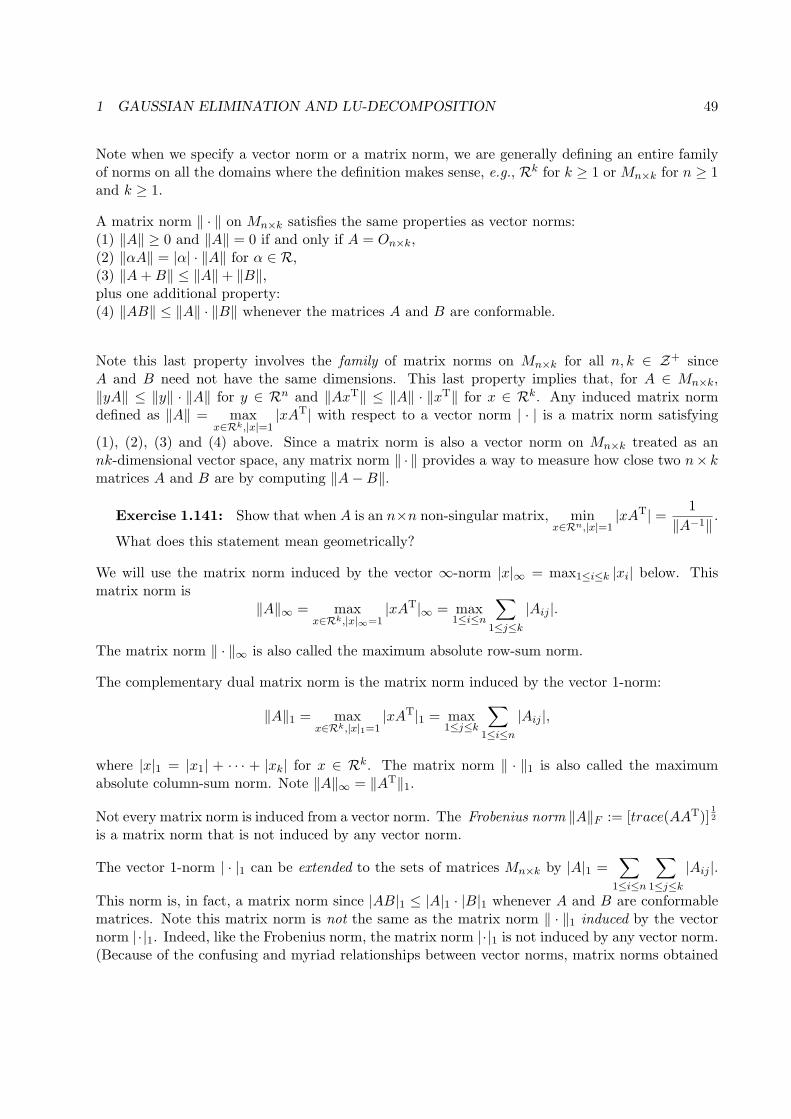
1 GAUSSIAN ELIMINATION AND LU-DECOMPOSITION 49
Note when we specify a vector norm or a matrix norm, we are generally defining an entire familyof norms on all the domains where the definition makes sense, e.g., Rk for k ≥ 1 or Mn×k for n ≥ 1and k ≥ 1.
A matrix norm ‖ · ‖ on Mn×k satisfies the same properties as vector norms:(1) ‖A‖ ≥ 0 and ‖A‖ = 0 if and only if A = On×k,(2) ‖αA‖ = |α| · ‖A‖ for α ∈ R,(3) ‖A + B‖ ≤ ‖A‖+ ‖B‖,plus one additional property:(4) ‖AB‖ ≤ ‖A‖ · ‖B‖ whenever the matrices A and B are conformable.
Note this last property involves the family of matrix norms on Mn×k for all n, k ∈ Z+ sinceA and B need not have the same dimensions. This last property implies that, for A ∈ Mn×k,‖yA‖ ≤ ‖y‖ · ‖A‖ for y ∈ Rn and ‖AxT‖ ≤ ‖A‖ · ‖xT‖ for x ∈ Rk. Any induced matrix normdefined as ‖A‖ = max
x∈Rk,|x|=1|xAT| with respect to a vector norm | · | is a matrix norm satisfying
(1), (2), (3) and (4) above. Since a matrix norm is also a vector norm on Mn×k treated as annk-dimensional vector space, any matrix norm ‖ · ‖ provides a way to measure how close two n× kmatrices A and B are by computing ‖A−B‖.
Exercise 1.141: Show that when A is an n×n non-singular matrix, minx∈Rn,|x|=1
|xAT| = 1
‖A−1‖ .What does this statement mean geometrically?
We will use the matrix norm induced by the vector ∞-norm |x|∞ = max1≤i≤k |xi| below. Thismatrix norm is
‖A‖∞ = maxx∈Rk,|x|∞=1
|xAT|∞ = max1≤i≤n
∑
1≤j≤k
|Aij |.
The matrix norm ‖ · ‖∞ is also called the maximum absolute row-sum norm.
The complementary dual matrix norm is the matrix norm induced by the vector 1-norm:
‖A‖1 = maxx∈Rk,|x|1=1
|xAT|1 = max1≤j≤k
∑
1≤i≤n
|Aij |,
where |x|1 = |x1| + · · · + |xk| for x ∈ Rk. The matrix norm ‖ · ‖1 is also called the maximumabsolute column-sum norm. Note ‖A‖∞ = ‖AT‖1.
Not every matrix norm is induced from a vector norm. The Frobenius norm ‖A‖F := [trace(AAT)]1
2
is a matrix norm that is not induced by any vector norm.
The vector 1-norm | · |1 can be extended to the sets of matrices Mn×k by |A|1 =∑
1≤i≤n
∑
1≤j≤k
|Aij |.
This norm is, in fact, a matrix norm since |AB|1 ≤ |A|1 · |B|1 whenever A and B are conformablematrices. Note this matrix norm is not the same as the matrix norm ‖ · ‖1 induced by the vectornorm |·|1. Indeed, like the Frobenius norm, the matrix norm |·|1 is not induced by any vector norm.(Because of the confusing and myriad relationships between vector norms, matrix norms obtained
1 GAUSSIAN ELIMINATION AND LU-DECOMPOSITION 50
by extending vector norms, and matrix norms induced by vector norms, alternate notations areoften employed to distinguish among such norms. For example, | · |, ‖ · ‖, and ||| · ||| are sometimesused for the three categories of norms listed above. Moreover, sometimes the notation |A| is usedto indicate the matrix whose (i, j)th element is |Aij |; we shall write abs(A) instead.)
Exercise 1.142: Show that the Frobenius norm is the extension of the Euclidean norm to
the sets of matrices Mn×k, i.e., ‖A‖F =
∑
1≤i≤n
∑
1≤j≤k
|Aij |2
1/2
. (This is not the same as the
matrix norm induced by the vector 2-norm.)
Exercise 1.143: Show that ‖x‖∞ = |x|1 and ‖x‖1 = |x|∞ for x ∈ Rn.
Exercise 1.144: Is the extension of the ∞-norm | · |∞ to Mn×k a matrix norm?
Exercise 1.145: Show that ‖ · ‖∞ is a matrix norm. Hint: show that maxp∑
h |Bph| ≤∑
h maxp |Bph| for B ∈Mk×m.
Solution 1.145: Let A be an n × k matrix and let B be an k ×m matrix. Then ‖AB‖∞ =
maxi
∑
h
|∑
j
AijBjh| ≤ maxi
∑
h
∑
j
|AijBjh| ≤ maxi
∑
j
maxp
∑
h
|Aij | · |Bjh|
≤
maxi
∑
j
|Aij |
(
maxp
∑
h
|Bph|)
. Note in particular, ‖xA‖∞ ≤ ‖x‖∞ ·‖A‖∞ where x ∈ Rn.
Exercise 1.146: Show that ‖ · ‖1 is a matrix norm.
An important property of vector and matrix norms is that all norms on a given finite-dimensionalvector space V are equivalent where two norms | · |a and | · |b are equivalent when there exist positive
constants µab and νab such that µab ≤|x|a|x|b
≤ νab for x ∈ V − {0}. This means we can convert
inequalities involving specified norms to similar inequalities involving other norms.
We can show that any two norms | · |a and | · |b on a finite-dimensional vector space V are equivalentas follows. Let Sb = {y ∈ V | |y|b = 1} and let µ = min
y∈Sb
|y|a. Note µ > 0 because Sb is closed and
bounded away from 0.
Now ifx
|x|b∈ Sb then |x|a = |x|b
∣
∣
∣
∣
x
|x|b
∣
∣
∣
∣
a
≥ |x|b miny∈Sb
|y|a = |x|bµ. Thus |x|a ≥ µ|x|b.
Similarly, let Sa = {y ∈ V | |y|a = 1} and let ν = miny∈Sa
|y|b. Note ν > 0.
Now ifx
|x|a∈ Sa then |x|b = |x|a
∣
∣
∣
∣
x
|x|a
∣
∣
∣
∣
b
≥ |x|a miny∈Sa
|y|b = |x|aν. Thus |x|b ≥ ν|x|a.
Therefore, µ|x|b ≤ |x|a ≤1
ν|x|b, and taking µab = µ and νab =
1
ν, we have µab ≤
|x|a|x|b
≤ νab for
x ∈ V − {0} where µab and νab are positive constants.
1 GAUSSIAN ELIMINATION AND LU-DECOMPOSITION 51
Exercise 1.147: Show that when the subscript a denotes the ∞-norm so that ‖A‖a = ‖A‖∞and the subscript b denotes the 1-norm so that ‖A‖b = ‖A‖1, then the equivalent-norm constantsrelating the norms ‖ · ‖a and ‖ · ‖b satisfy µab = νba and νab = µba. For ‖ · ‖∞ and ‖ · ‖1 on Mn×n,
we have µab =1
nand νab = n. Thus
1
n‖A‖∞ ≤ ‖A‖1 ≤ n‖A‖∞ and
1
n‖A‖1 ≤ ‖A‖∞ ≤ n‖A‖1
for A ∈Mn×n.
Exercise 1.148: Show that ‖A‖1 ≤ |A|1 ≤ n‖A‖1 for A ∈Mn×n.
Now returning to the analysis of errors in the solution of a set of linear equations, let xA = v, andassume we have computed an approximation x to x using LU-decomposition and back-substitution.Also suppose we have an n× k matrix E such that x(A + E) = v. In other words, we look at x asthe exact solution of a “nearby” system of linear equations, as well as an approximate solution ofthe given system of linear equations.
This “natural” idea can be realized, i.e., such a matrix E always exists when x 6= 0, (generallymany error matrices exist such that x(A + E) = v.) We compute x which “solves” xA = v witherror. Thus xA = v + v for some vector v. Now we introduce a matrix E such that xE = −v.Note this is always possible when x 6= 0. Then x(A + E) = v. This introduction of an error matrixis possible for any consistent linear system of equations xA = v where the computed solution x isnon-zero. (Note if x is close to 0 and v is far from 0, E may need to be large.)
Introducing an error matrix E “converts” the error in x to become error in A instead. Thiserror matrix E is now taken to be due to the round-off error that occurs in computing the LU-decomposition of A and using back-substitution to compute x.
For the purpose of error analysis, we may assume the permutation matrices P and Q that bring thepivot elements of A onto the diagonal are identity matrices since permuting rows and columns duringthe computation for L and U introduces no errors. Thus, for the purpose of error analysis, we mayassume A is “pre-permuted” and we may write LU = A and similarly write the LU-decompositionof A computed with fixed finite-precision arithmetic in terms of error matrices without permutationmatrix factors.
The Gaussian-elimination LU-decomposition algorithm applied to the n×n non-singular matrix Agenerates two sequences of matrices: L(1) = A, L(2), . . ., L(n) = L and U (1) = I, U (2), . . ., U (n) = U ,where L(h+1) and U (h+1) are computed in iteration h. When fixed finite-precision arithmetic isused, corresponding sequences L(1) = A, L(2), . . ., L(n) = L and U (1) = I, U (2), . . ., U (n) = U arecomputed instead, where L(h) and U (h) correspond to L(h) and U (h) with round-off error included.Thus the LU-decomposition of A computed with fixed finite-precision arithmetic consists of alower-triangular matrix L and an upper-triangular matrix U with diag(U) = (1, 1, . . . , 1) such thatLU = A + A for some error matrix A (under our assumption that A is “pre-permuted”, and nopivot search is used.)
Let the error matrices L and U be defined by L+ L = L and U + U = U . Then A = LU +LU + LU .Note when L and U are uniquely determined by A, the error matrix A is also uniquely determinedby A since L and U are uniquely determined by A by their construction.
Further error is introduced when computing x by back-substitution. Specifically, we want to solveyU = v and xL = y, and, with fixed finite-precision arithmetic, this results in y and x where
1 GAUSSIAN ELIMINATION AND LU-DECOMPOSITION 52
y(U + U ′) = v and x(L + L′) = y. The error matrices L′ and U ′ are due to round-off error in theback-substitution computation.
Thus x(L+L′)(U+U ′) = v. Let L = L+L′ and U = U+U ′. Then, in terms of these combined errormatrices, we have x(L+L)(U +U) = v and thus A+E = (L+L)(U +U) = LU +LU +LU +LU , soE = LU +LU +LU . Altogether then, x can be taken as an exact vector that satisfies x(A+E) = v.
Exercise 1.149: Show that a specific error matrix E such that x(A+E) = v can be computed
in terms of x, A, and v as E =xTd
xxTwhere d = v − xA.
When we study how close the matrix A + E is to A, i.e., how “big” E is, we are doing a backwardserror analysis. We are transferring our attention from the problem of estimating the error in xcaused by round-off error to the problem of what nearby problem has x as its exact solution andhow close together the original problem and the nearby problem are.
If A + E is sufficiently close to A for A in some class of matrices W then we say that our LU-decomposition and back-substitution algorithm for solving systems of linear equations is (back-wards) stable for inputs (A, v) ∈W ×Rk; this means that, for the problem xA = v, our algorithmoutputs the exact solution to a quantifiably-nearby problem. This is realistically the most we canhope for in the presence of round-off error. (The stability class W depends on what we take “suffi-cently close” to mean.) Note, since the matrix E such that x(A + E) = v is not generally unique,we may restrict our choice of E to be minimal in some matrix norm if desired.
Exercise 1.150: Suppose W1 is the class of matrices for which Gaussian-elimination LU-decomposition with minimal pivoting is stable (according to some fixed criterion.) And supposeW2 is the class of matrices for which Gaussian-elimination LU-decomposition with cross-rowpartial pivoting is stable (using the same criterion,) and W3 is the class of matrices for whichGaussian-elimination LU-decomposition with complete pivoting is stable (again using the samecriterion.) Is it the case that W1 ⊆W2 ⊆W3?
Our LU-decomposition and back-substitution algorithm often yields a small residual v − xA when(A, v) ∈W×Rk. However having |v−xA| small does not guarantee that the relative error |x−x|/|x|in the computed solution x is small. For the relative error to be small, other conditions on thematrix A must hold. It is also possible to have a large residual and a small relative error.
Now let us take k = n so that A is a square matrix, and let A be non-singular. Then with Anon-singular, we can obtain Wilkinson’s bound [Wil63] [IK66] [DB74] [GV89] [Mey00]:
‖E‖∞ ≤ k2(n)u · ‖A‖∞,
where u is the rounding-unit of our floating-point number system and where k2(n) = (3n3 +2n2)gn
with gn ≤ 2n−1 when cross-column partial-pivoting is used. This bound is sharp, i.e., this boundis attained for certain n × n matrices when the exact value of gn is used as defined below. And
gn ≤ n1
2
[
2 · 3 1
2 · · ·n1
n−1
] 1
2 ≤ 2n1/2nlog(n)/4 when complete-pivoting is used. When rook-pivoting
is employed, Foster shows that gn ≤ 1.5n4+3 log(n)/4 which is comparible to the complete-pivotingbound [Fos97]. (Recall that the rounding-unit u is the smallest positive floating-point value such
1 GAUSSIAN ELIMINATION AND LU-DECOMPOSITION 53
that 1+u > 1 in machine arithmetic. The associated “binary-precision” is p = 1− log2(u) bits andthe corresponding decimal precision is [1− log2(u)]/ log2(10) digits.)
The function gn is defined with respect to the sequence of matrices A(h) = Rh · · ·R1AC1M1 · · ·ChMh
+E(h) for h = 1, . . . , n arising in the iterations of the LU-decomposition algorithm where E(h) is thematrix of errors introduced during iterations 1 through h by using fixed finite-precision arithmetic.Recall that for the purpose of error analysis, we may take the permutation matrices R1, . . ., Rn andC1, . . ., Cn to be identity matrices. (Note A(h) = L(h) where the matrices A = L(1), L(2), . . . , L(n)
are computed in the successive iterations of the Gaussian-elimination LU-decomposition algorithmusing fixed finite-precision arithmetic.) Specifically, assuming A has computational rank n, so thatthe LU-decomposition algorithm has n iterations, we have
gn =
max1≤h≤n
max1≤i≤n1≤j≤n
|A(h)ij |
/
max1≤i≤n1≤j≤n
|Aij |
.
The function gn measures the relative “growth” of elements in the sequence of matrices A(1), A(2),. . ., A(n), (i.e., L(1), L(2), . . ., L(n),) and specifically, gn bounds the relative growth in the suc-cessive pivot values used in the Gaussian-elimination LU-decomposition algorithm, when fixedfinite-precision arithmetic is used.
The value gn depends on the choice of pivot values; this is why the bounds for gn are differentfor complete-pivoting and partial-pivoting. (We require A have computational rank n to avoidan undefined gn multiplier value.) (Since with either cross-column partial-pivoting or complete-pivoting, |Uij | ≤ 1, it is the potential growth in the intermediate results in L(h) for h = 1, 2, . . . , nthat we are concerned with.
Exercise 1.151: We have |Uij | ≤ 1. Do we also have |Uij | ≤ 1, where U is the estimate of Ucomputed with fixed finite-precision arithmetic. Hint: look at the definition of rounding with
the rounding unit u: round(2mf) = sign(f) · 2m · u ·⌊ |f |
u+
1
2
⌋
where f = 0 or1
2≤ |f | < 1 and
m ∈ Z.
(When round(2mf) is to be involved in a further computation with other rounded numbers, a
better statistically-unbiased rounding formula is obtained by treating the case|f |u
mod 1 =1
2
specially. If|f |u
mod 1 =1
2, we add
1
2to|f |u
to round up only if the integer u
⌊ |f |u
⌋
is odd;
otherwise we add 0.)
Although sharp, Wilkinson’s bound is almost always conservative. Also the bounds for the functiongn given above are generally far too large; for complete-pivoting gn is a slow-growing function of n,and empirically, for most matrices, gn < 10 for n < 400 even for partial-pivoting [GV89] [DB74].(Does gn → ∞ as n → ∞, either with ‖A‖∞ < α for α fixed or when ‖A‖∞ is unconstrained andthe elements of A are randomly-chosen according to some convenient (semi-realistic) distribution,when complete-pivoting is employed?) Prior to 1992 it was conjectured that gn ≤ n for complete-pivoting, however, counterexamples have been provided by Edelman [Ede92]. Obtaining a tighter
1 GAUSSIAN ELIMINATION AND LU-DECOMPOSITION 54
bound on gn, potentially given in terms of the elements of the matrix A, is one of the outstandingproblems in numerical analysis.
Note as a practical matter, we could directly compute gn for any particular matrix A while executingthe LU-decomposition algorithm.
Wilkinson’s bound directly indicates how far the matrix A + E is from the matrix A, and thusWilkinson’s bound allows us to define the class W of matrices for which we will deem LU-decomposition and back-substitution to be stable in terms of the values n and ‖A‖∞.
With the non-singular matrix A “pre-permuted” so that A is a diagonal-pivot matrix and no pivotsearch is required, then starting with L(1) = A, and using exact arithmetic, the Gaussian-eliminationLU-decomposition algorithm generates the sequence of matrices L(1), L(2), . . ., L(n) = L, as well asthe sequence of matrices U (1) = In×n, U (2), . . ., U (n) = U using the successive diagonal elements
L(1)11 , L
(2)22 , . . . as pivot values. The elements of U are accumulated row by row, and once entered in
U (h) are never changed; and most importantly, |Uij | ≤ 1. The elements of the matrices L(1), L(2),. . ., L(n) = L, however, may grow large in magnitude as the LU-decomposition algorithm progressesiteration by iteration.
Wilkinson’s bound arises from looking closely at the error in the output L and U of the Gaussian-elimination LU-decomposition algorithm using fixed finite-precision arithmetic. To do this we mustexamine the errors in the sequence of matrices L(1), L(2), . . ., L(n) = L, and in the matrix U (n) = U ,where L(h) is the estimate of the matrix L(h) and U (h) is the similar estimate of the matrix U (h)
obtained with fixed finite-precision arithmetic. Recall that with exact arithmetic, we have:
L(h+1)ij =
0 for i ≤ h and j > i,
L(h)ij for j ≤ h and i ≥ j,
L(h)ij − Uhj · L(h)
ih for j > h and i > h,
and Uij =
0 for i > j,1 for i = j,
L(i)ij
L(i)ii
for i < j.
When fixed finite-precision arithmetic is used, we compute the matrices L and U rather than Land U , and we have:
L(h+1)ij =
0 for i ≤ h and j > i,
L(h)ij for j ≤ h and i ≥ j,[
L(h)ij − Uhj · L(h)
ih · (1 + α(h+1)ij u)
]
(1 + β(h+1)ij u) for j > h and i > h,
and U(h+1)ij =
0 for i < j,1 for i = j,[
L(i)ij
L(i)jj
]
(1 + γ(h+1)ij u) for i < j,
where u is our rounding unit and 1 + α(h)ij u, 1 + β
(h)ij u, and 1 + γ
(h)ij u, with |α(h)
ij | ≤ 1, |β(h)ij | ≤ 1,
and |γ(h)ij | ≤ 1, are values that encode the rounding done in the operations they multiply during
iteration h. Recall U = U (n).
1 GAUSSIAN ELIMINATION AND LU-DECOMPOSITION 55
We may convert our accounting for error in L(h+1)ij to additive error by writing
L(h+1)ij =
0 for i ≤ h and j > i,
L(h)ij for j ≤ h and i ≥ j,
L(h)ij − Uhj · L(h)
ih + ǫ(h+1)ij for j > h and i > h,
and we may show that |ǫ(h+1)ij | ≤ 2gnu max
i,j|Aij | for i > h + 1, j > h + 1.
By looking at the error matrix A = LU − A, and using the recursion relation L(h+1)ij = L
(h)ij −
Uhj · L(h)ih + ǫ
(h+1)ij for j > h and i > h, we can obtain |Aij | =
∑
1≤h≤i
|ǫ(h+1)ij | for i < j and |Aij | =
∑
1≤h<j
|ǫ(h+1)ij | for i ≥ j. Let α = maxi,j |Aij |. Then the bound |ǫ(h+1)
ij | ≤ 2gnuα for i > h + 1,
j > h + 1 yields |Aij | ≤{
i2αgnu for i < j,(j − 1)2αgnu for i ≥ j,
so ‖A‖∞ ≤ n(n− 1)αgnu.
Now we may bound the magnitudes of the elements of the error matrix T ′ accounting for theround-off error in solving an n× n lower-triangular system xT = y by back-substitution (i.e.,x(T + T ′) = y.) This bound is |T ′
ij | ≤ max(2, |i − j + 1|) · |Tij | · u with nu ≤ 1. We can use
this bound together with the bound on ‖A‖∞ to obtain Wilkinson’s bound: ‖E‖∞ ≤ k2(n)u‖A‖∞where k2(n) = (3n3 + 2n2)gn. A full proof of Wilkinson’s bound is given in [IK66].
We know from practice and experience that using a minimal pivot search results in large errorsrelatively often; thus we take it as accepted that LU-decomposition and back-substitution withminimal-pivoting is unstable outside a relatively-small class of inputs. For any chosen stabil-ity criteria, the stability class for LU-decomposition and back-substitution with minimal-pivotingis much smaller than the stability class for LU-decomposition and back-substitution with eitherpartial-pivoting or complete-pivoting.
Note both LU-decomposition and back-substitution with complete-pivoting and LU-decompositionand back-substitution with partial-pivoting become less stable as n → ∞. More precisely, theclass of matrices for which either algorithm is stable diminishes in size as n→∞, but the class ofmatrices for which LU-decomposition and back-substitution with partial-pivoting is stable shrinksin size much faster than the class of matrices for which complete-pivoting is stable.
There are two relative errors we may consider: |x − x|/|x| is the forward relative error of x and|x− x|/|x| is the backward relative error of x with respect to the vector norm | · |. (We assume thatx 6= 0 and x 6= 0.) These relative error quantities are related.
Specifically, define δ by δ|x| = |x− x| and define γ by γ|x| = |x− x| where | · | is a generic vectornorm. Then δ = |∆|/|x|, and γ = |∆|/|x| where ∆ = x − x. Note |∆| = | − ∆|. Thus δ is theforward relative error of x and γ is the backward relative error of x with respect to the vector norm
| · |. Also,δ
1 + δ=
|∆|/|x|1 + |∆|/|x| =
|∆||x|+ |∆| ≤
|∆||x| = γ since |x| = |x + ∆| ≥ |x| + |∆|. Similarly,
γ
1 + γ=
|∆|/|x|1 + |∆|/|x| =
|∆||x|+ |∆| ≤
|∆||x| = δ.
1 GAUSSIAN ELIMINATION AND LU-DECOMPOSITION 56
Exercise 1.152: Show that |x−x|1/|x|1 = ‖x−x‖∞/‖x‖∞ and |x−x|∞/|x|∞ = ‖x−x‖1/‖x‖1.
Now to obtain a bound on the backward relative error |x− x|/|x| = |∆|/|x| where ∆ = x− x, wemay proceed as follows.
Suppose n = k and suppose A is non-singular. We have xA = v and x(A + E) = v = (x + ∆)(A +E) = xA + xE + ∆A + ∆E, so ∆A + xE = 0. Thus ∆ = −xEA−1, so for any generic matrix norm‖ · ‖, we have ‖∆‖ ≤ ‖x‖ · ‖E‖ · ‖A−1‖, and thus
‖∆‖‖x‖ ≤ κ(A)
‖E‖‖A‖
where κ(A) = ‖A‖ · ‖A−1‖.
The value κ(A) is called the condition number of the non-singular matrix A with respect to thematrix norm ‖ · ‖. (In some circumstances we can take κ(A) = ‖A‖ · ‖A+‖ for arbitrary n × kmatrices where A+ is the Moore-Penrose pseudo-inverse of A.) Note the condition number κ isdependent on the matrix norm employed. When we have a specific norm ω in mind, we shall writeκω.
Note when we take our generic matrix norm to be ‖ · ‖∞, Wilkinson’s bound yields
‖∆‖∞‖x‖∞
≤ κ∞(A)k2(n)u.
This inequality shows that the backward relative error in x measured with respect to the maximum-absolute-rowsum matrix norm is small when n and the condition number κ∞(A) are not too large.If the ∞-matrix norm of the matrix of measurement errors in the coefficient matrix A is greaterthan k2(n)uκ∞(A) then we may justifiably claim that x is as accurate as possible since we startwith an uncertainty equal to or greater than that produced by round-off error.
Now since |z|1 = ‖z‖∞ and |z|∞ = ‖z‖1 for z ∈ Rn, it is convenient to let the vector norm | · |denote the vector norm | · |1 and the matrix norm ‖ · ‖ denote the matrix norm ‖ · ‖∞, or let thevector norm | · | denote the vector norm | · |∞ and the matrix norm ‖ · ‖ denote the matrix norm‖ · ‖1. Then, with this understanding,
|∆||x| =
‖∆‖‖x‖ ≤ κ(A)
‖E‖‖A‖
where κ(A) = ‖A‖ · ‖A−1‖.
Exercise 1.153: Show that|∆||x| ≤
‖v − xA‖‖x‖ · ‖A‖ . Hint: ‖x− x‖ ≤ ‖v − xA‖ · ‖A−1‖.
Now recall|∆||x| = γ ≥ δ/(1 + δ). Let β = κ(A)
‖E‖‖A‖ . Then β ≥ γ and thus β ≥ δ/(1 + δ). Thus
(1 + δ)β ≥ δ so (β − 1)δ ≥ −β and (1 − β)δ ≤ β. Now if β = κ(A)‖E‖‖A‖ < 1, then δ ≤ β/(1 − β).
1 GAUSSIAN ELIMINATION AND LU-DECOMPOSITION 57
Thus we have the upper bound κ(A)‖E‖‖A‖ /
(
1− κ(A)‖E‖‖A‖
)
for the forward relative error|∆||x| when
κ(A)‖E‖‖A‖ < 1, i.e., when 1− κ(A)
‖E‖‖A‖ = 1− β > 0 with A non-singular, we have
|∆||x| ≤ κ(A)
‖E‖‖A‖ /
(
1− κ(A)‖E‖‖A‖
)
=κ(A)‖E‖
‖A‖ − κ(A)‖E‖ =κ(A)
‖A‖/‖E‖ − κ(A)
where | · | and ‖ · ‖ are either | · |1 and ‖ · ‖∞, or | · |∞ and ‖ · ‖1, respectively. (β < 1 is equivalentto ‖A−1‖ · ‖E‖ < 1, and this implies A + E is non-singular.)
As κ(A) or ‖E‖ or both increase so that κ(A)‖E‖‖A‖ approaches 1, this bound approaches ∞, (and
if κ(A)‖E‖‖A‖ ≥ 1,
|∆||x| is potentially unbounded, i.e., A + E might be singular.)
If we fix our matrix norm to be ‖ · ‖∞, and use Wilkinson’s bound and assume the maximum
amount of round-off error occurs so that ‖E‖∞ = k2(n)u‖A‖∞, then‖∆‖∞‖x‖∞
≤ κ∞(A)k2(n)u/(1−
κ∞(A)k2(n)u) when κ∞(A) <1
k2(n)u. This reveals that with µ ∈ (0,∞), if κ∞(A) <
1
k2(n)u· µ
1 + µ
then‖∆‖∞‖x‖∞
≤ µ.
Exercise 1.154: Let α = k2(n)u and let µ ∈ (0,∞). Show that, with | · | = | · |1, δ ≤ µ when
κ∞(A) ≤ 1
α· µ
1 + µ.
A matrix A for which κ(A) is large is called ill-conditioned. A system of linear equations xA = vwith an ill-conditioned coefficient matrix and a non-zero righthand-side vector has the property thata small change in A can produce a large change in the computed solution x. An ill-conditioned setof linear equations is essentially a set of linearly-dependent or almost linearly-dependent equations.(We should make every effort to avoid having to compute a solution for xA = v where A has lessthan full rank.) When the rows of A are “robustly” independent, the condition number κ(A) willnot be large.
If a sufficiently-small pivot value arises during execution of the LU-decomposition algorithm thenthe coefficient matrix A is ill-conditioned. The converse is not true. A matrix A may not have anyoverly-small or overly-large non-zero elements, and it may be that the magnitudes of all the pivotvalues that arise are far from zero, but still κ(A) is large.
Exercise 1.155: Let the n × n matrix B =
1 0 · · · 0−1 1 0 · · · 0−1 −1 1 · · · 0
......
. . .. . . 0
−1 −1 · · · −1 1
. Show that B−1 is
defined by (B−1))ij = 0 for i < j, (B−1))ij = 1 for i = j, and (B−1))ij = 2i−1−j for i > j. Thenshow that κ∞(B) = κ1(B) = n · 2n−1.
REFERENCES 58
This example shows that a nice-looking matrix like B, whose pivot values for either minimal-pivoting, cross-column partial-pivoting, or complete-pivoting, are all of similar magnitude canhave a large condition number. Although computing a solution to xB = v can be done exactlyor almost exactly, computing a solution to x(B + P ) = v, for P a perturbation matrix withsmall elements is much more problematic for large n.
In order to assess the condition of a matrix A we need to estimate κ(A) = ‖A‖ · ‖A−1‖ using somematrix norm. If we had to compute A−1 it would be costly, and also potentially unreliable if κ(A)were in fact large. Golub and Van Loan [GV89] discuss an O(n2) algorithm for estimating κ∞(A),and with this algorithm we have a reasonable (but not guaranteed) way to assess the relative error(either forward or backward) in a computed solution x of the linear system xA = v by estimatingthe relevant relative error upper-bound with respect to the ∞ matrix norm. (Experiments showthat we may generally take k2(n) ≤ 10 when n ≤ 100, however this is not guaranteed.) Anotherway to assess the relative error in x is to perturb A, re-solve xA = v, and see if the new x is closeto or far from the old x.
Exercise 1.156: Explain why round-off error will generally cause the computational rank ofan n× n coefficient matrix to be the value n when the LU-decomposition algorithm is applied.
Since‖∆‖∞‖x‖∞
≤ 10
2pκ∞(A) is usually approximately true when p is the binary precision of our
floating-point format, we may define ‘ill-conditioned’ as κ∞(A) > 2p/2, say. In general we canexpect h-decimal-digit accuracy in x when κ∞(A) < 2d−h where d = p log2(10), and we cannotexpect h-decimal-digit accuracy otherwise.
We have xA = v and x(A + E) = v so the residual d := v − xA = v − x(A + E) + xE = xE andthus ‖d‖ ≤ ‖x‖ · ‖E‖. For A non-singular, Wilkinson’s bound yields ‖d‖∞ ≤ k2(n)u‖A‖∞‖x‖∞.
Since this bound on the length of the residual depends on ‖x‖∞ as well as ‖A‖∞, and does notdirectly depend on κ∞(A), we see that the size of d is not well-correlated with the accuracy of x
as measured by either the forward relative error‖∆‖∞‖x‖∞
or the backward relative error‖∆‖∞‖x‖∞
.
Exercise 1.157: Show that d = −∆A where ∆ = x− x and show that ‖∆‖ ≥ ‖d‖/‖A‖.
Exercise 1.158: (Dahlquist [DB74]) Assume xA = v where A is an n×n non-singular matrixand v 6= 0. Define e by xA = v + e where x is the approximate solution of xA = v producedby the LU-decomposition and back-substitution algorithm with complete-pivoting. (Here weascribe the result of round-off error to be equivalent to a perturbation of the righthand-sidevector v.)
Let ∆ = x− x. Show that ‖∆‖ ≤ ‖A−1‖ · ‖e‖. Show that‖∆‖‖x‖ ≤ κ(A)
‖e‖‖v‖ = κ(A)
‖v − xA‖‖v‖ .
References
[DB74] Germund Dahlquist and Ake Bjørck. Numerical Methods. Prentice-Hall, 1974.
REFERENCES 59
[DJM06] Froilan Dopico, Charles Johnson, and Juan Molera. Multiple LU factorizations of asingular matrix. Lin. Alg. and its Applications, (419):24–36, 2006.
[Ede92] Alan Edelman. The complete pivoting conjecture for Gaussian elimination is false. TheMathematica Journal, 2:58–61, 1992.
[Fos97] Leslie V. Foster. The growth factor and efficiency of Gaussian elimination with rookpivoting. J. Computational and Applied Math., 86(1):177–194, 1997.
[Grc11a] Joseph F. Grcar. How ordinary elimination became Gausssian elimination. HistoriaMath., 38:163–218, 2011.
[Grc11b] Joseph F. Grcar. John von Neumann’s analysis of Gausssian elimination and the originsof modern numerical analysis. SIAM Review, 53(4):607–682, 2011.
[GV89] Gene H. Golub and Charles F. Van Loan. Matrix Computations, second edition. JohnHopkins University Press, 1989.
[IK66] Eugene Issacson and Herbert Bishop Keller. Analysis of Numerical Methods. Wiley,New York, 1966.
[Knu73] Donald E. Knuth. The Art of Computer Programming: Volume 1, Fundamental Algo-rithms, second edition. Addison-Wesley, New York, 1973.
[Knu97] Donald E. Knuth. The Art of Computer Programming: Volume 2, Seminumerical Al-gorithms. Addison-Wesley, New York, 1997.
[Mey00] Carl D. Meyer. Matrix Analysis and Applied Linear Algebra. SIAM, 2000.
[NP92] Larry Neal and George Poole. A geometric analysis of gaussian elimination II. LinearAlgebra Appl., 173:249–272, 1992.
[OJ97] Pavel Okunev and Charles R. Johnson. Necessary and sufficient conditions for existenceof the LU factorization of an arbitrary matrix. arxiv.org, technical report, Dept. ofMathematics, College of William and Mary, July 1997.
[ON96] Markus Olschowka and Arnold Neumaier. A new pivoting strategy for Gaussian elimi-nation. Linear Algebra Appl., 240:131–151, 1996.
[PTVF92] William H. Press, Saul A. Teukolsky, William T. Vetterling, and Brian P. Flannery. Nu-merical Recipes in FORTRAN - The Art of Scientific Computing (2nd. ed.). CambridgeUniv. Press, N.Y., 1992.
[Smi10] Jane Smiley. The Man who invented the Computer: the Biography of John Atanasoff.Doubleday, New York, 2010.
[vNG47] John von Neumann and Herman H. Goldstine. Numerical inverting of matrices of highorder. Bull. Amer. Math. Soc., 53:1021–1099, 1947.
[Wil63] James H. Wilkinson. Rounding Errors in Algebraic Processes. Prentice-Hall, 1963.

![[7] Gaussian Elimination - Coding The Matrix · Gaussian Elimination [7] Gaussian Elimination. Starting to peek inside the black box So far solve(A, b) is a black box. With Gaussian](https://img.pdfslide.net/doc/110x75/5ba1840309d3f2bb6a8c8421/7-gaussian-elimination-coding-the-gaussian-elimination-7-gaussian-elimination.jpg)