HAL Id: hal-01497824https://hal.archives-ouvertes.fr/hal-01497824

Preprint submitted on 13 Apr 2017

HAL is a multi-disciplinary open accessarchive for the deposit and dissemination of sci-entific research documents, whether they are pub-lished or not. The documents may come fromteaching and research institutions in France orabroad, or from public or private research centers.

L’archive ouverte pluridisciplinaire HAL, estdestinée au dépôt et à la diffusion de documentsscientifiques de niveau recherche, publiés ou non,émanant des établissements d’enseignement et derecherche français ou étrangers, des laboratoirespublics ou privés.

Gendered internal migration patterns in SenegalIsabelle Chort, Philippe de Vreyer, Thomas Zuber

To cite this version:Isabelle Chort, Philippe de Vreyer, Thomas Zuber. Gendered internal migration patterns in Senegal.2017. �hal-01497824�

UMR DIAL 225

Place du Maréchal de Lattre de Tassigny 75775 • Paris •Tél. (33) 01 44 05 45 42 • Fax (33) 01 44 05 45 45

• 4, rue d’Enghien • 75010 Paris • Tél. (33) 01 53 24 14 50 • Fax (33) 01 53 24 14 51

E-mail : dial@dial.prd.fr • Site : www.dial.ird

DOCUMENT DE TRAVAIL DT/2017-02

DT/2016/11

Gendered internal migration patterns in Senegal

Health Shocks and Permanent Income Loss: the Household Business Channel

Isabelle CHORT

Philippe DE VREYER

Thomas ZUBER

Axel Demenet

Gendered internal migration patterns in Senegal∗

Isabelle Chort† Philippe De Vreyer‡ Thomas Zuber §

Abstract

Using individual panel data from Senegal collected in 2006-07 and 2010-12,this study explores internal migration patterns of men and women. The data usedcontain the GPS coordinates of individuals’ location, allowing us to calculate precisemigration distances and map individual mobilities.Women are found to be morelikely to migrate than men. However, they move less far and are more likely tomigrate to rural areas, especially when originating from rural areas. Educationis found to increase the likelihood of migration to urban destinations, especiallyfor women. An analysis of the motives for migrating confirms the existence ofgendered migration patterns, as female mobility is mostly linked to marriage whilelabor mobility is frequently observed for men.

Keywords : Internal migration; gender inequalities; rural-urban migration; SenegalJEL classification : R23; J16; O15; O18

∗We are grateful to Joachim Jarreau and Karine Marazyan for helpful comments and suggestions.†Universite Paris-Dauphine, PSL Research University, LEDa, DIAL, 75016 Paris, France; Institut

de Recherche pour le Developpement, UMR DIAL, 75010 Paris, France. Address: LEDa, UniversiteParis-Dauphine, Place du Marechal de Lattre de Tassigny, 75775 PARIS Cedex 16, France. Email:isabelle.chort@dauphine.fr.‡Universite Paris-Dauphine, PSL Research University, LEDa, DIAL, 75016 Paris, France; Institut de

Recherche pour le Developpement, UMR DIAL, 75010 Paris, France§PhD Candidate, Columbia University. Department of Middle Eastern, South Asian and African

Studies/History, New York, NY, 10027.

1

1 Introduction

Studies on migration have favored the analysis of international movements and their

dynamics. However, largely due to physical, financial and psychological costs, the vast

majority of population movements take place within national boundaries (UNDP, 2009).

While internal migration is generally under-documented, this is even more striking in

the context of developing countries, especially in Sub-Saharan Africa. Moreover gender

differences in access to migration have been little explored. The few studies that have

focused on this issue have stressed the limited geographic mobility of women, explained by

gender roles or family constraints (Kanaiaupuni, 2000; Assaad and Arntz, 2005; Massey,

Fischer, and Capoferro, 2006; Chort, 2014). Yet, internal migration plays an important

role in social mobility by providing access to employment opportunities (Assaad and

Arntz, 2005; De Brauw, Mueller, and Lee, 2014). Uncovering the different determinants

of women’s and men’s migration patterns can contribute to reduce the gap between male

and female migration rate by informing policies aimed at promoting labor-market oriented

female mobility.

The aim of this paper is to study the gender-specific determinants of internal migra-

tion and distance travelled in Senegal. We use individual panel data from a nationally

representative survey collected in 2006-2007 and 2010-2012 (Poverty and Family Struc-

ture survey). Our data are unique first in that all individuals in the household are tracked,

within the country boundaries, whatever their relationship to the household head. They

thus provide us with a direct information on internal migration, which is rare in develop-

ing countries, and even more in sub-Saharan Africa (De Brauw, Mueller, and Lee, 2014).

Second, our data contain the GPS coordinates of individuals’ location in both waves.

We are thus able to calculate distances precisely and map individual mobilities, avoiding

limitations and constraints of migration definitions based on administrative units. In

addition, the PSF survey includes several modules containing valuable demographic and

economic information at the individual, household, and community levels, which allows

2

us to analyze a large set of economic and non-economic determinants of internal mobility.

We use in addition data from the 2002 Senegalese census to investigate the role of migra-

tion “push-factors” at the sub-regional level (departement). The econometric analysis of

the determinants of migration decision, distance travelled and rural or urban location is

complemented with a descriptive study of migration motives and a mapping of individual

moves using cartographic tools.

The econometric analysis first reveals that women are more likely to migrate than men.

A careful analysis of attrition between the two survey waves nuances this observation as

the attrition rate is significantly higher for men, which suggests that women who migrate

are less likely than men to live alone and be lost with their entire household, or to lose

contact with their origin household. Consistent with this interpretation, we find that the

distance travelled is significantly lower for women than for men. We find that women

are more likely than men to experience rural-to-rural migration and that for women this

kind of migration is associated with marriage. Importantly, education is found to increase

both men and women’s probability of migrating to urban areas.

This article makes several contributions. First, it increases our knowledge of Sene-

galese internal migration by providing a comprehensive picture of internal migration and

its determinants in contemporary Senegal based on individual panel data. By combining

survey and census data this article simultaneously considers individual, household, com-

munity and regional determinants of migration and distance travelled. This study thus

complements and extends the analysis by Herrera and Sahn (2013) who focus only on

Senegalese youth (21-35 year old) and measure internal migration based on retrospective

data collected in 2003.

Second, this article focuses on gender differences in internal migration patterns which

have been largely overlooked. An analysis of migration motives declared in our data (see

Figure 3) reveals drastic differences between men and women. A large share of female

migration is driven by family motives, the most important of them being marriage. By

contrast, the proportion of women migrating for labor-related reasons is low, while labor

3

is the primary migration motive for men. Such observations suggest little evolution in

the last 30 years, as the conclusion by Chant et al. (1992) based on numerous case

studies in the developing world are unchallenged: in contemporary Senegal, women are

less likely than men to migrate independently for employment. This specific feature of

female internal migration being largely associated with marriage is common to many

sub-Saharan African countries (Kudo, 2015) and probably explains in part the relative

lack of interest of the economic literature for female mobility since Thadani and Todaro

(1984).

More specifically, this articles links gender-specific migration patterns to the analysis

of rural-urban mobility. Regarding internal migrations in sub-Saharan Africa, studies

have nuanced the overwhelming focus on rural-to-urban mobility and have highlighted

the importance of rural-to-rural migration (Beauchemin and Bocquier, 2004; Beauchemin,

2011; Bocquier and Mukandila, 2013). Recent research suggest that the urbanization rate

in the region has been overstated (Potts, 2012). Rural out-migration has been slowing in

the recent decades, and even reversing in some countries (Beauchemin, 2011; Potts, 2009).

Rural-urban migration rates in sub-Saharan Africa are lower than the microeconomic

theory would predict given the large and positive income differentials between urban and

rural areas (De Brauw, Mueller, and Lee, 2014). It is argued here that the observed

rural-to-rural patterns in our data have a strong gender component. Female mobility

appears to be constrained, more limited geographically, and in a large part subordinate to

family reasons. However, the fact that education is found to increase women’s likelihood

of migrating to urban destinations, suggests possible channels to overcome barriers to

female migration.

Third, the current state of the literature allows this paper to provide rare insight

into the dynamics of migration and distance within the context of a developing country.

Indeed, recent research has tried to grapple with limitations of migration data aggre-

gated by administrative units (Bell et al., 2015). In developed countries, the rationales

for migration have been found to differ depending on distance travelled: whereas short-

4

distance mobility is associated with housing and life-cycle motives, long-distance migra-

tion is driven by employment motivations (Cordey-Hayes and Gleave, 1974; Clark and

Huang, 2004; Niedomysl and Fransson, 2014). To our knowledge, this article provides the

first study using migration distances based on GPS coordinates in sub-Saharan Africa.

Interestingly, our findings are rather consistent with the above categories, but we add

to this strand of literature by showing that they are strongly linked to gender-specific

migration paradigms. We tend to observe a predominance of short-distance rural-rural

marriage-related migrations among women, and more diverse patterns for men with a

non-negligible share of long-distance labor-related migration to urban destinations driven

by the unrivaled attractiveness of the capital city, Dakar.

Last, together with econometric analysis, the cartographic tools used in this article

contribute to highlighting the role of migration hub played by Dakar and provide a vivid

illustration of the different types of mobility associated with the declared motives for

migrating.

The next section describes the data used. Section 3 presents our empirical methodol-

ogy. Section 4 presents the econometric results for the determinants of internal migration

rural/urban migration and distance traveled, depending on gender, and discusses attrition

issues. Finally Section 5 concludes.

2 Data

2.1 The PSF Individual Panel Survey

The data used in this study come from the two waves of the “Poverty and Family Struc-

ture” Survey (PSF), conducted in Senegal in 2006-07 for the first wave, and from late 2010

to the beginning of 2012 for the second wave1. The sample in the first wave is nationally

1The survey has been conducted by a team of French researchers and researchers from the NationalStatistical Agency of Senegal and is described in detail in DeVreyer et al. (2008). Momar Sylla andMatar Gueye of the Agence Nationale de la Statistique et de la Demographie of Senegal (ANSD) on theone hand and Philippe De Vreyer (Paris-Dauphine Dauphine, IRD-DIAL), Sylvie Lambert (PSE) andAbla Safir (World Bank) designed the survey. The data have been collected by the ANSD thanks to the

5

representative and made of 1750 households (14,450 individuals), in 150 randomly drawn

census districts. All individuals surveyed in the first wave have been tracked, except when

abroad, forming an individual panel. The attrition rate between the two waves is 11.6%.

As attrition may result in a great part from internal migration, issues related to attrition

are carefully discussed in Section 4.4.

The PSF surveys are particularly suited to the study of internal migration since

they provide the exact location of individuals through GPS coordinates in both waves

of the panel. Thanks to these coordinates, we calculate Euclidean distances traveled by

individuals between the two waves 2.

The PSF data contain in addition rich information on individual and household socio-

demographic characteristics, and on community infrastructures, which allows us to finely

document the determinants of internal migration. In particular, consumption data are

collected for each household subgroup referred to as a cell. Cells are semi-autonomous

consumption units including a cell head and all her dependents (in particular her children,

foster children and widowed mother or father). The average number of cells per household

is 2.51 3. We are thus able to account for consumption at both the household and cell

levels. We include in all our regressions variables for the household and cell size, and

for the relative consumption of the cell. To complement objective wealth indicators and

account for relative deprivation as a potential driver of internal migration, we use two

distinct questions about the perceived wealth of the household on the one hand, and

the community on the other, with 5 modalities each (from “very poor” to “very rich”).

Households are classified as “richer” than their community if their self-assessed wealth

level is higher than the one reported for their community.

funding of the IDRC (International Development Research Center), INRA Paris and CEPREMAP.2While Senegalese geography offers further complexity when it comes to using Euclidean distances,

due to the position of the Gambia along the Gambia river, Euclidean measurement is the most relevantand accessible means of computing distances of internal migration (Bell et al., 2002). Note in additionthat most mobility observed from and to the area south of the Gambia, the Casamance, made of theregions of Ziguinchor and Kolda, is connected to the capital city Dakar, as shown in Figure 1. The citiesof Dakar and Ziguinchor are connected once more by ferry since 2005, after the dramatic sinking of LeJoola in 2002, and very few travellers choose the land route. The Euclidean distance thus seems to be arelevant proxy for the travel distance even from and to the regions of Senegal south of the Gambia.

3See Lambert, Ravallion, and van de Walle (2014) for a more detailed description of cell definition.

6

We used in addition data from a 10% sample of the 2002 Senegalese census to calculate

indicators of poverty and inequality4 at the county level, based on 2006 administrative

boundaries 5. Figure 6 in Appendix shows the geographic distribution of the computed

poverty and inequality statistics at the county level.

2.2 Descriptive Statistics

The present analysis focuses on individuals 15 years and older, as the mobility of younger

individuals is more likely to be decided on by their parents and subject to specific mo-

tives6. Therefore, the initial database is reduced to a panel of 6,986 individuals (8,636

including attritors, individuals deceased between the two waves and those migrating

abroad). To avoid the inherent problems of administrative geography (Bell et al., 2015),

our definition of internal migrants is based on the distance between the two locations

calculated from recorded GPS coordinates. We use 5km as a lower bound for internal

migration as very short-distance moves may be partly caused by measurement errors.

Moreover, the 5km threshold represents in the Senegalese context a significant enough

distance that there are costs attached to this mobility. As a robustness check, other

cutoffs where chosen (see Table 6 in Appendix where the definition of internal migrants

is based on a 10km cutoff). Based on Euclidean distances, 670 individuals moved of more

than 5km between the first and second wave of the survey.

Migrants account for 9.6% of individuals tracked in the panel. Descriptive statistics

in the Appendix present characteristics of individuals and of their household in the first

wave of the survey, which are relevant for understanding the determinants of migration

between the two survey waves. When including all types of migration (internal and

international), internal migration accounts for 69% of migrants, making it a significant

4Both measures were obtained using the PovMap2 software developed by the World Bank (Zhao andLanjouw, 2009; Elbers, Lanjouw, and Lanjouw, 2003)

5Senegal was subdivided into 34 counties (departements) in 11 regions in 2006. In 2008, Senegalunderwent administrative reforms: the country is currently subdivided into 45 counties (departements)and 14 regions.

6Child fostering, in particular, is widespread in Senegal (Beck et al., 2011)

7

phenomenon to study. As appears in Table 4, migrants are more likely to be women

(58.6% compared to 55.3% for non-migrants), they tend to be better educated (29.1%

have a secondary education or higher compared to 19% among non-migrants) and are

younger (66.5% are under 30 compared to 46.3% for non-migrants).

Regarding the geography of internal migrations, the data reveal the overwhelming

polarity and attractiveness of Dakar. Indeed 16.1% of internal migrants in our data come

from Dakar, while 21% move to Dakar between the two survey waves (excluding Intra-

Dakar mobility). In addition, intra-Dakar mobility (of more than 5km) represents 17.3%

of internal migration. Overall, internal migrants going to or from Dakar represent 37.2%

of all migrants (54.4% including intra-Dakar mobility) while the Dakar metropolitan area

accounts for 20% of the Senegalese population in 2002 (ANSD (Agence Nationale de la

Statistique et de la Demographie), 2006). As a robustness check, we exclude intra-Dakar

migrants from our sample of internal migrants, since mobility within the community of

Dakar, even though on a distance larger than 5km, might not be considered migration.

Table 5 in Appendix focuses on rural/urban migratory dynamics and confirms the

intensity of migration to urban centers, with 70% of internal migrants moving to urban

settings. Particularly notable is the intensity of migration from urban-to-urban settings

which accounts for 77% of migrations for individuals originating in urban areas. This

should be in part nuanced by the intensity of mobility within the region of Dakar, which

accounts for 41% of all urban-to-urban mobility. This intensity of intra-Dakar mobility

finds parallels with part of the argument made by Beauchemin and Bocquier (2004)

on migration and urbanization whereby intra-urban mobility (and its peri-urban spaces,

which are Pikine and Guediawaye for Dakar) better explains urban expansion than in-

migration initially.

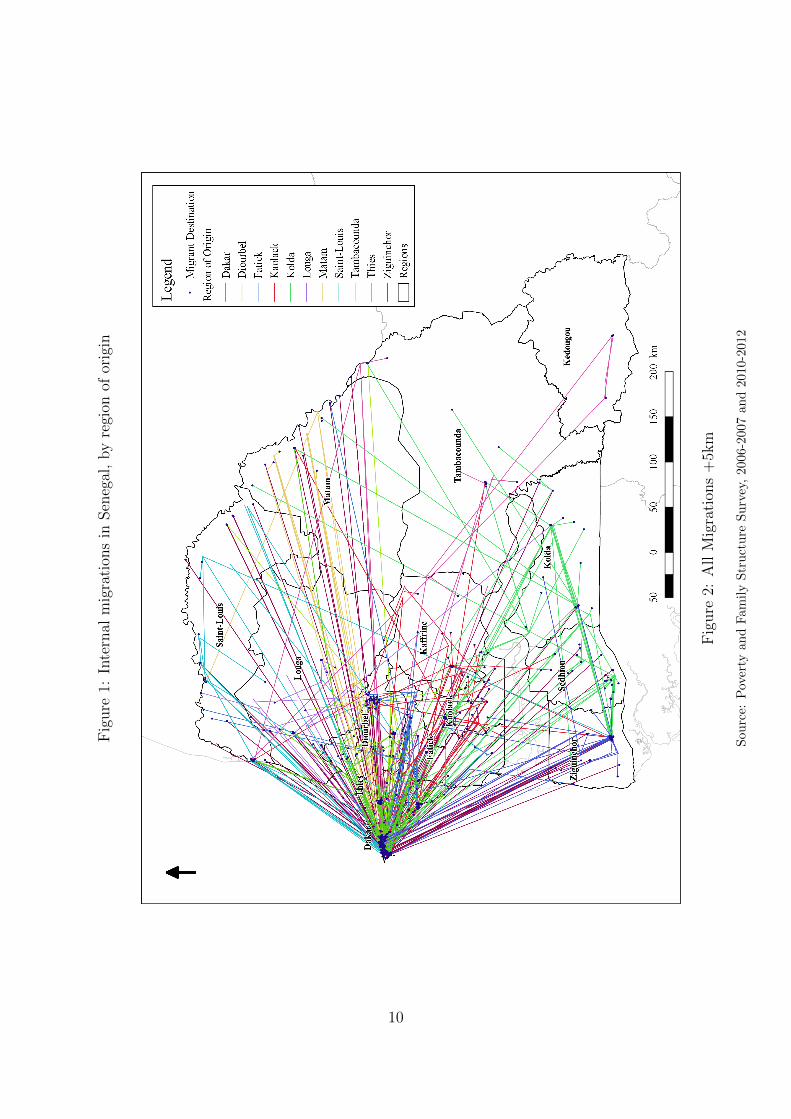
Figure 1 represents individual mobilities between the two survey waves, based on GPS

coordinates. Different colors materialize the different regions of origin while dots represent

destinations. The attractiveness of Dakar is illustrated by the numerous lines converging

towards the capital city. Interestingly, Dakar is strongly connected to all Senegalese

8

regions, including that of Ziguinchor in spite of its relative geographic isolation. The

cities of Thies and Touba, in the region of Thies and Diourbel respectively, also appear

as major destinations, mostly from nearby regions - 58% of all migrants were found in

Dakar, Thies and Diourbel, emphasizing the weight of the Dakar-Touba axis. Additional

maps by type of origin and destination, rural or urban (Figure 4), by gender and migration

motive (Figure 5) are provided in Appendix.

9

Fig

ure

1:In

tern

alm

igra

tion

sin

Sen

egal

,by

regi

onof

orig

in

Fig

ure

2:A

llM

igra

tion

s+

5km

Sou

rce:

Pov

erty

an

dF

am

ily

Str

uct

ure

Su

rvey

,2006-2

007

and

2010-2

012

10

Figure 3 shows the distribution of reasons for migration across distance travelled

and reveals a striking contrast with regards to reasons for moving between women and

men. Regardless of distance, 40 to 60% women’s mobility is explained by marriage or

return to spousal home. Employment and education are marginal migration motives for

women and appear only for medium to long distances. By contrast, except for very short

distances (under 50km), 40 to 66% of male migration is explained by either education or

employment.

3 Empirical approach

3.1 Empirical models

In line with the individual models of migration derived from Todaro (1997) explaining

migration decision by earning differentials we explore the role of individual variables such

as gender, age, education or socio-professional category in the migration decision. We

account for the contributions of the literature initiated by Stark and Bloom (1985) and

Rosenzweig and Stark (1989) that emphasized the household dimension of the migration

decision by considering individuals’ relative position in the household. We control in

particular for the relationship to the household head and for the birth rank among siblings

as previous research in the case of Senegal has shown that elders are more likely to migrate

as they are expected to send more remittances (Chort and Senne, 2015). In addition, we

investigate the question of relative deprivation as a potential driver of migration (Stark,

1984; Stark and Taylor, 1989) at three different levels. At the household level first, we

exploit the rich data on consumption disaggregated at the cell (household subgroup) level

to proxy for the relative economic status and/or bargaining power within the household.

Second, we use subjective data on household wealth compared to the perceived average

wealth of the community. Finally, we explore the impact of inequality at the county level,

as, according to Stark (1984), we should observe more migration where the distribution of

income is more unequal. Building on the literature focusing on the impact of the quality

11

of amenities on migration (Dustmann and Okatenko, 2014), we control for the availability

of education and health services in the community.

We estimate a probit model for migration decision :

IntMigrant∗i = α + β′Xi + εi (1)

where IntMigrant∗i is a latent variable only observed as:

IntMigranti = 1{IntMigrant∗i>0} (2)

IntMigranti is a dummy variable equal to one if individual i has migrated internally

between the two survey waves. More precisely, internal migrants are defined as indi-

viduals surveyed in the second wave at a location distant of more than 5km from their

initial location. As robustness checks, we use a 10km threshold instead and we exclude

mobilities within the capital city of Dakar (see Tables 6 and 7 in Appendix). Note that

for lack of exhaustive retrospective information on individual migration trajectories, we

cannot account for temporary mobility that occurred between the two survey waves, i.e.

individuals who migrated and settled back in their household of origin. Xi is a set of

individual, household, community and county (departement) characteristics. Individual

variables include gender, age, education, ethnicity, dummies for having been fostered

before the age of 15 and for first-borns, relationship to the household head, and socio-

professional status. Household controls are the size of the household, a consumption

index per adult equivalent, the size of the cell, the ratio between cell consumption and

household consumption and a measure of self-reported wealth within the community.

Community determinants include controls for the environment (urban or rural) and

public services (public hospital, primary and secondary schools). Finally, two variables

are defined at the county (departement) level: a measure of poverty (headcount) and a

12

measure of inequality (Gini index). εi is an individual specific error term. We estimate

our model on the pooled sample (men and women) and separately for each gender, as we

expect migration determinants to vary across gender.

Second, on the sample of migrants, we investigate the determinants of distance trav-

elled by estimating the following equation with OLS:

LnDISTi,w1−w2 = γ + δ′Xi + νi (3)

where LnDISTi,w1−w2 denotes the log of the Euclidian distance between locations of in-

dividual at waves 1 and 2, computed based on the GPS coordinates collected by the

surveyors. Xi is the same set of individual, household, community and county character-

istics than in equation 1 and νi is an error term.

Finally, we estimate a multinomial logit model to investigate the issue of rural/urban

migrations. Instead of considering the binary decision to migrate or stay, we model the

three-option choice to migrate to an urban area, to a rural area, or stay.

4 Empirical findings

4.1 Determinants of migration

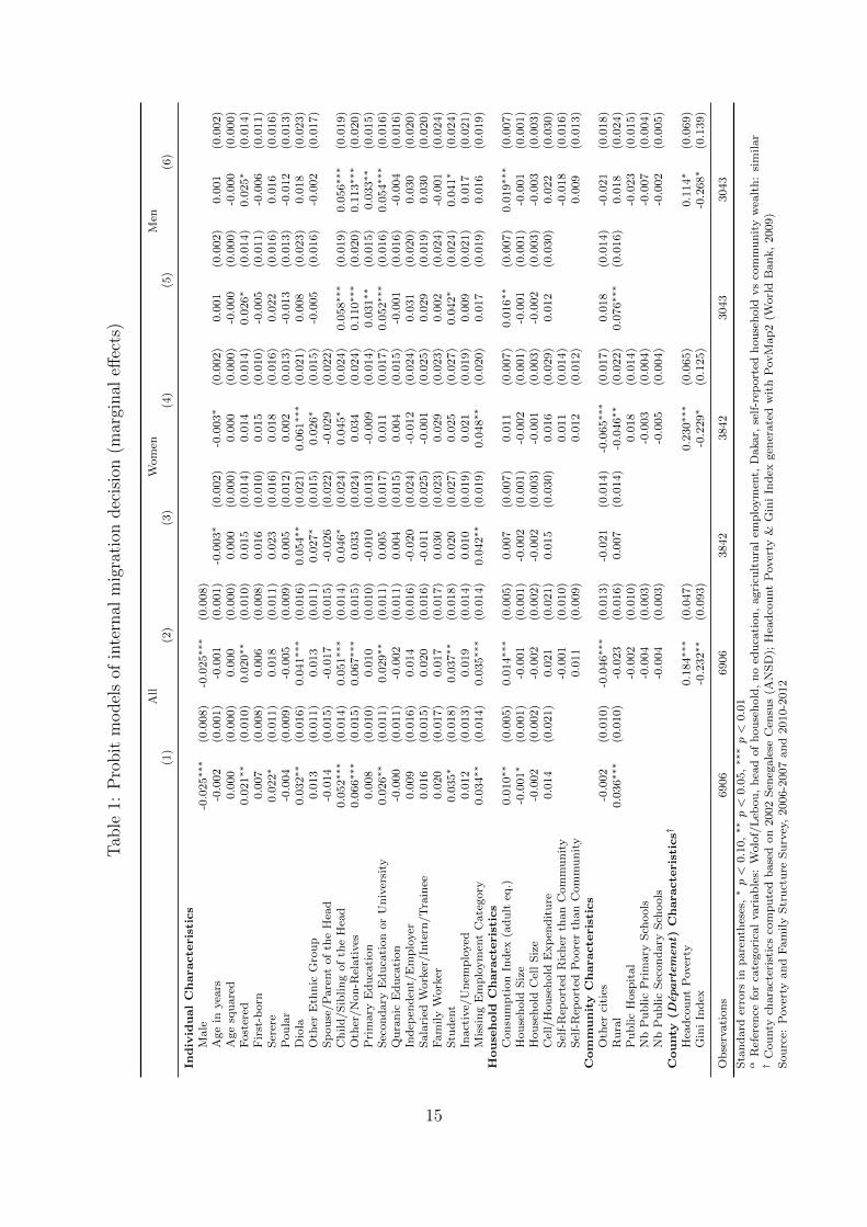
Table 1 presents the estimation results of a Probit model for internal migration decision

on the whole sample (columns 1 and 2), and separately for women (column 3 and 4) and

men (columns 5 and 6). According to our definition of internal migrants, the dependent

variable is a dummy equal to one for individuals who were living in the second survey

wave in a household distant of more than 5km from their household in wave 1. In addition

to individual and household determinants of migration, specifications shown in columns

2, 4 and 6 include migration push-factors at the community and county level.

As a robustness check, we used an alternative threshold of 10km for the definition

13

of migrants. The results are very similar, as shown in Table 6 in Appendix. Moreover,

to avoid mixing intra-urban relocation and internal migration, we replicated the analysis

excluding individuals moving within the capital city of Dakar, irrespective of the distance.

Results are shown in Table 7 in Appendix.

Since the decision to migrate within the country and abroad are probably intercon-

nected, we estimated a multinomial logit model for migration with three alternatives:

stay (the reference), migrate internally, or migrate abroad. Results are shown in Table 13

and are remarkably close to those obtained in our main specifications, with only marginal

differences in the coefficients on the ethnicity dummies.

As mentioned above, attrition is a major concern as we expect internal migration to

be the major cause of attrition between the two survey waves. We provide regression

results including attrition in Table 12 and discuss further attrition issues in Section 4.4.

14

Tab

le1:

Pro

bit

model

sof

inte

rnal

mig

rati

ondec

isio

n(m

argi

nal

effec

ts)

All

Wom

enM

en(1

)(2

)(3

)(4

)(5

)(6

)

Individ

ualCharacte

ristics

Male

-0.0

25∗∗∗

(0.0

08)

-0.0

25∗∗∗

(0.0

08)

Age

inyea

rs-0

.002

(0.0

01)

-0.0

01

(0.0

01)

-0.0

03∗

(0.0

02)

-0.0

03∗

(0.0

02)

0.0

01

(0.0

02)

0.0

01

(0.0

02)

Age

squ

are

d0.0

00

(0.0

00)

0.0

00

(0.0

00)

0.0

00

(0.0

00)

0.0

00

(0.0

00)

-0.0

00

(0.0

00)

-0.0

00

(0.0

00)

Fost

ered

0.0

21∗∗

(0.0

10)

0.0

20∗∗

(0.0

10)

0.0

15

(0.0

14)

0.0

14

(0.0

14)

0.0

26∗

(0.0

14)

0.0

25∗

(0.0

14)

Fir

st-b

orn

0.0

07

(0.0

08)

0.0

06

(0.0

08)

0.0

16

(0.0

10)

0.0

15

(0.0

10)

-0.0

05

(0.0

11)

-0.0

06

(0.0

11)

Ser

ere

0.0

22∗

(0.0

11)

0.0

18

(0.0

11)

0.0

23

(0.0

16)

0.0

18

(0.0

16)

0.0

22

(0.0

16)

0.0

16

(0.0

16)

Pou

lar

-0.0

04

(0.0

09)

-0.0

05

(0.0

09)

0.0

05

(0.0

12)

0.0

02

(0.0

13)

-0.0

13

(0.0

13)

-0.0

12

(0.0

13)

Dio

la0.0

32∗∗

(0.0

16)

0.0

41∗∗∗

(0.0

16)

0.0

54∗∗

(0.0

21)

0.0

61∗∗∗

(0.0

21)

0.0

08

(0.0

23)

0.0

18

(0.0

23)

Oth

erE

thn

icG

rou

p0.0

13

(0.0

11)

0.0

13

(0.0

11)

0.0

27∗

(0.0

15)

0.0

26∗

(0.0

15)

-0.0

05

(0.0

16)

-0.0

02

(0.0

17)

Sp

ou

se/P

are

nt

of

the

Hea

d-0

.014

(0.0

15)

-0.0

17

(0.0

15)

-0.0

26

(0.0

22)

-0.0

29

(0.0

22)

Ch

ild

/S

iblin

gof

the

Hea

d0.0

52∗∗∗

(0.0

14)

0.0

51∗∗∗

(0.0

14)

0.0

46∗

(0.0

24)

0.0

45∗

(0.0

24)

0.0

58∗∗∗

(0.0

19)

0.0

56∗∗∗

(0.0

19)

Oth

er/N

on

-Rel

ati

ves

0.0

66∗∗∗

(0.0

15)

0.0

67∗∗∗

(0.0

15)

0.0

33

(0.0

24)

0.0

34

(0.0

24)

0.1

10∗∗∗

(0.0

20)

0.1

13∗∗∗

(0.0

20)

Pri

mary

Ed

uca

tion

0.0

08

(0.0

10)

0.0

10

(0.0

10)

-0.0

10

(0.0

13)

-0.0

09

(0.0

14)

0.0

31∗∗

(0.0

15)

0.0

33∗∗

(0.0

15)

Sec

on

dary

Ed

uca

tion

or

Un

iver

sity

0.0

26∗∗

(0.0

11)

0.0

29∗∗

(0.0

11)

0.0

05

(0.0

17)

0.0

11

(0.0

17)

0.0

52∗∗∗

(0.0

16)

0.0

54∗∗∗

(0.0

16)

Qu

ran

icE

du

cati

on

-0.0

00

(0.0

11)

-0.0

02

(0.0

11)

0.0

04

(0.0

15)

0.0

04

(0.0

15)

-0.0

01

(0.0

16)

-0.0

04

(0.0

16)

Ind

epen

den

t/E

mp

loyer

0.0

09

(0.0

16)

0.0

14

(0.0

16)

-0.0

20

(0.0

24)

-0.0

12

(0.0

24)

0.0

31

(0.0

20)

0.0

30

(0.0

20)

Sala

ried

Work

er/In

tern

/T

rain

ee0.0

16

(0.0

15)

0.0

20

(0.0

16)

-0.0

11

(0.0

25)

-0.0

01

(0.0

25)

0.0

29

(0.0

19)

0.0

30

(0.0

20)

Fam

ily

Work

er0.0

20

(0.0

17)

0.0

17

(0.0

17)

0.0

30

(0.0

23)

0.0

29

(0.0

23)

0.0

02

(0.0

24)

-0.0

01

(0.0

24)

Stu

den

t0.0

35∗

(0.0

18)

0.0

37∗∗

(0.0

18)

0.0

20

(0.0

27)

0.0

25

(0.0

27)

0.0

42∗

(0.0

24)

0.0

41∗

(0.0

24)

Inact

ive/

Un

emp

loyed

0.0

12

(0.0

13)

0.0

19

(0.0

14)

0.0

10

(0.0

19)

0.0

21

(0.0

19)

0.0

09

(0.0

21)

0.0

17

(0.0

21)

Mis

sin

gE

mp

loym

ent

Cate

gory

0.0

34∗∗

(0.0

14)

0.0

35∗∗∗

(0.0

14)

0.0

42∗∗

(0.0

19)

0.0

48∗∗

(0.0

20)

0.0

17

(0.0

19)

0.0

16

(0.0

19)

House

hold

Characte

ristics

Con

sum

pti

on

Ind

ex(a

du

lteq

.)0.0

10∗∗

(0.0

05)

0.0

14∗∗∗

(0.0

05)

0.0

07

(0.0

07)

0.0

11

(0.0

07)

0.0

16∗∗

(0.0

07)

0.0

19∗∗∗

(0.0

07)

Hou

seh

old

Siz

e-0

.001∗

(0.0

01)

-0.0

01

(0.0

01)

-0.0

02

(0.0

01)

-0.0

02

(0.0

01)

-0.0

01

(0.0

01)

-0.0

01

(0.0

01)

Hou

seh

old

Cel

lS

ize

-0.0

02

(0.0

02)

-0.0

02

(0.0

02)

-0.0

02

(0.0

03)

-0.0

01

(0.0

03)

-0.0

02

(0.0

03)

-0.0

03

(0.0

03)

Cel

l/H

ou

seh

old

Exp

end

itu

re0.0

14

(0.0

21)

0.0

21

(0.0

21)

0.0

15

(0.0

30)

0.0

16

(0.0

29)

0.0

12

(0.0

30)

0.0

22

(0.0

30)

Sel

f-R

eport

edR

ich

erth

an

Com

mu

nit

y-0

.001

(0.0

10)

0.0

11

(0.0

14)

-0.0

18

(0.0

16)

Sel

f-R

eport

edP

oore

rth

an

Com

mu

nit

y0.0

11

(0.0

09)

0.0

12

(0.0

12)

0.0

09

(0.0

13)

Com

munity

Characte

ristics

Oth

erci

ties

-0.0

02

(0.0

10)

-0.0

46∗∗∗

(0.0

13)

-0.0

21

(0.0

14)

-0.0

65∗∗∗

(0.0

17)

0.0

18

(0.0

14)

-0.0

21

(0.0

18)

Ru

ral

0.0

36∗∗∗

(0.0

10)

-0.0

23

(0.0

16)

0.0

07

(0.0

14)

-0.0

46∗∗

(0.0

22)

0.0

76∗∗∗

(0.0

16)

0.0

18

(0.0

24)

Pu

blic

Hosp

ital

-0.0

02

(0.0

10)

0.0

18

(0.0

14)

-0.0

23

(0.0

15)

Nb

Pu

blic

Pri

mary

Sch

ools

-0.0

04

(0.0

03)

-0.0

03

(0.0

04)

-0.0

07

(0.0

04)

Nb

Pu

blic

Sec

on

dary

Sch

ools

-0.0

04

(0.0

03)

-0.0

05

(0.0

04)

-0.0

02

(0.0

05)

County

(Depart

em

en

t)Characte

ristics†

Hea

dco

unt

Pover

ty0.1

84∗∗∗

(0.0

47)

0.2

30∗∗∗

(0.0

65)

0.1

14∗

(0.0

69)

Gin

iIn

dex

-0.2

32∗∗

(0.0

93)

-0.2

29∗

(0.1

25)

-0.2

68∗

(0.1

39)

Ob

serv

ati

on

s6906

6906

3842

3842

3043

3043

Sta

nd

ard

erro

rsin

pare

nth

eses

,∗p<

0.1

0,∗∗p<

0.0

5,∗∗∗p<

0.0

1α

Ref

eren

cefo

rca

tegori

cal

vari

ab

les:

Wolo

f/L

ebou

,h

ead

of

hou

seh

old

,n

oed

uca

tion

,agri

cult

ura

lem

plo

ym

ent,

Dakar,

self

-rep

ort

edh

ou

seh

old

vs

com

mu

nit

yw

ealt

h:

sim

ilar

†C

ou

nty

chara

cter

isti

csco

mp

ute

db

ase

don

2002

Sen

egale

seC

ensu

s(A

NS

D);

Hea

dco

unt

Pover

ty&

Gin

iIn

dex

gen

erate

dw

ith

PovM

ap

2(W

orl

dB

an

k,

2009)

Sou

rce:

Pover

tyan

dF

am

ily

Str

uct

ure

Su

rvey

,2006-2

007

an

d2010-2

012

15

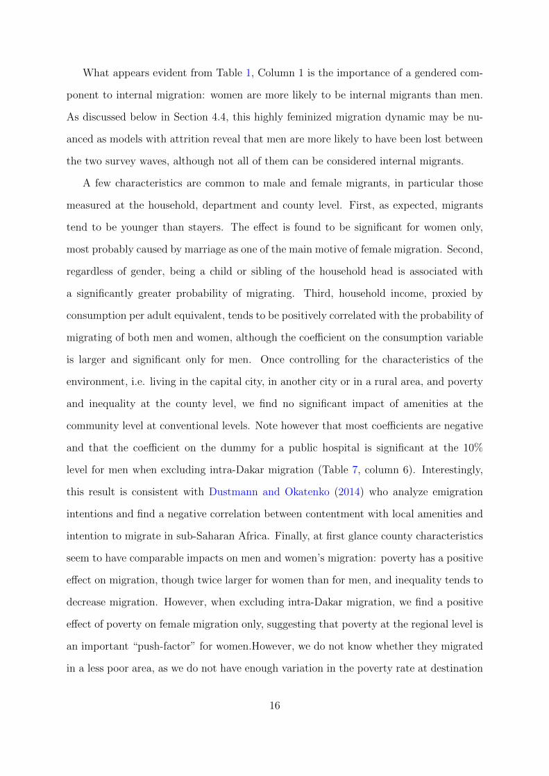
What appears evident from Table 1, Column 1 is the importance of a gendered com-

ponent to internal migration: women are more likely to be internal migrants than men.

As discussed below in Section 4.4, this highly feminized migration dynamic may be nu-

anced as models with attrition reveal that men are more likely to have been lost between

the two survey waves, although not all of them can be considered internal migrants.

A few characteristics are common to male and female migrants, in particular those

measured at the household, department and county level. First, as expected, migrants

tend to be younger than stayers. The effect is found to be significant for women only,

most probably caused by marriage as one of the main motive of female migration. Second,

regardless of gender, being a child or sibling of the household head is associated with

a significantly greater probability of migrating. Third, household income, proxied by

consumption per adult equivalent, tends to be positively correlated with the probability of

migrating of both men and women, although the coefficient on the consumption variable

is larger and significant only for men. Once controlling for the characteristics of the

environment, i.e. living in the capital city, in another city or in a rural area, and poverty

and inequality at the county level, we find no significant impact of amenities at the

community level at conventional levels. Note however that most coefficients are negative

and that the coefficient on the dummy for a public hospital is significant at the 10%

level for men when excluding intra-Dakar migration (Table 7, column 6). Interestingly,

this result is consistent with Dustmann and Okatenko (2014) who analyze emigration

intentions and find a negative correlation between contentment with local amenities and

intention to migrate in sub-Saharan Africa. Finally, at first glance county characteristics

seem to have comparable impacts on men and women’s migration: poverty has a positive

effect on migration, though twice larger for women than for men, and inequality tends to

decrease migration. However, when excluding intra-Dakar migration, we find a positive

effect of poverty on female migration only, suggesting that poverty at the regional level is

an important “push-factor” for women.However, we do not know whether they migrated

in a less poor area, as we do not have enough variation in the poverty rate at destination

16

due to the high share of internal migrants going to Dakar 7. This finding is also consistent

with the persistence of traditional practices of marriage-related female migration in the

poorest and most remote areas of the country. This issue is further discussed in the

following sections.

Separate regressions for men and women reveal numerous differences in the individual

migration determinants of the two groups. Having been fostered is associated with a

significantly higher probability of internal migration for men only. This finding is in line

with the literature on fostering as a household strategy aimed at increasing children’s

social mobility which could be associated with a greater geographic mobility in adulthood.

The difference across genders is linked to the different motives behind boys and girls’

fostering, as women are more likely to be fostered into households in which they will be

married (Beck et al., 2011).

Ethnicity is found to be correlated with female migration only. Women belonging to

Diola ethnic group and, to a lesser extent, to the Serere ethnic group are more likely to

migrate than members of the Senegalese largest Wolof ethnic group. This finds parallels

in the work of Brockerhoff and Eu (1993) documenting mobility by Serere and Diola

women to urban regions for domestic work.

As for education, we find that men with at least some primary education are more

likely to become internal migrants than those with no education at all (Table 1, Column

5-6), while for women, no significant differences in migration propensities are observed

depending on educational level.

4.2 Migration distance

7Although there is variation in the poverty rate within Dakar between poor areas like Guediawaye andrich ones such as the Almadies, the 10% extract of the 2002 census that we could exploit does not allowus to construct poverty measure at a finer level of disaggregation than the county level (departement).The same limitations applies to our county-level inequality measure which is included as a “push” factoronly.

17

Tab

le2:

Det

erm

inan

tsof

mig

rati

ondis

tance

-O

LS

esti

mat

ion

(sam

ple

:ad

ult

mig

rants

(+15

year

s)>

5km

)

All

Wom

enM

en(1

)(2

)(3

)(4

)(5

)(6

)

Individ

ualCharacte

ristics

Male

0.4

16∗∗∗

(0.1

21)

0.4

50∗∗∗

(0.1

18)

Age

inyea

rs0.0

02

(0.0

20)

-0.0

04

(0.0

20)

0.0

27

(0.0

26)

0.0

15

(0.0

26)

-0.0

38

(0.0

34)

-0.0

28

(0.0

34)

Age

squ

are

d-0

.000

(0.0

00)

0.0

00

(0.0

00)

-0.0

00

(0.0

00)

-0.0

00

(0.0

00)

0.0

00

(0.0

00)

0.0

00

(0.0

00)

Fost

ered

-0.1

63

(0.1

44)

-0.2

15

(0.1

40)

-0.0

54

(0.2

01)

-0.0

88

(0.2

00)

-0.3

52∗

(0.2

09)

-0.4

24∗∗

(0.2

03)

Fir

st-b

orn

-0.1

62

(0.1

15)

-0.1

42

(0.1

12)

-0.3

12∗∗

(0.1

56)

-0.2

90∗

(0.1

53)

0.0

22

(0.1

68)

0.0

61

(0.1

65)

Ser

ere

-0.0

40

(0.1

70)

0.0

79

(0.1

65)

0.1

94

(0.2

33)

0.2

27

(0.2

27)

-0.3

07

(0.2

51)

-0.1

40

(0.2

46)

Pou

lar

0.2

65∗

(0.1

38)

0.1

46

(0.1

40)

0.2

47

(0.1

85)

0.0

93

(0.1

88)

0.3

37

(0.2

08)

0.1

91

(0.2

13)

Dio

la0.3

45

(0.2

23)

0.0

96

(0.2

22)

0.2

82

(0.3

06)

0.1

39

(0.3

09)

0.4

36

(0.3

41)

0.0

40

(0.3

37)

Oth

eret

hn

icgro

up

0.2

22

(0.1

73)

-0.0

01

(0.1

74)

0.3

88∗

(0.2

26)

0.1

23

(0.2

29)

0.0

29

(0.2

71)

-0.1

66

(0.2

77)

Sp

ou

se/P

are

nt

of

the

Hea

d-0

.034

(0.2

55)

0.0

91

(0.2

48)

-0.2

64

(0.3

78)

-0.0

77

(0.3

71)

Ch

ild

/S

iblin

gof

the

Hea

d0.3

35

(0.2

44)

0.4

26∗

(0.2

38)

0.1

37

(0.3

97)

0.2

46

(0.3

91)

0.2

23

(0.3

43)

0.2

75

(0.3

35)

Oth

er/N

on

-Rel

ati

ves

0.4

21∗

(0.2

47)

0.4

53∗

(0.2

40)

0.2

87

(0.3

93)

0.3

42

(0.3

86)

0.2

81

(0.3

56)

0.3

33

(0.3

48)

Pri

mary

Ed

uca

tion

-0.2

81∗

(0.1

48)

-0.3

83∗∗∗

(0.1

45)

-0.2

93

(0.1

96)

-0.4

12∗∗

(0.1

95)

-0.2

89

(0.2

36)

-0.3

02

(0.2

30)

Sec

on

dary

Ed

uca

tion

or

Un

iver

sity

-0.5

23∗∗∗

(0.1

71)

-0.6

45∗∗∗

(0.1

66)

-0.1

59

(0.2

39)

-0.2

88

(0.2

36)

-0.7

37∗∗∗

(0.2

53)

-0.7

87∗∗∗

(0.2

46)

Qu

ran

icE

du

cati

on

-0.0

15

(0.1

72)

-0.0

10

(0.1

68)

-0.1

32

(0.2

28)

-0.0

82

(0.2

25)

0.0

94

(0.2

77)

0.0

64

(0.2

69)

Ind

epen

den

t/E

mp

loyer

0.2

41

(0.2

57)

0.2

50

(0.2

50)

-0.0

76

(0.4

08)

-0.0

28

(0.4

06)

0.5

17

(0.3

25)

0.4

45

(0.3

17)

Sala

ried

Work

er/In

tern

/T

rain

ee0.2

16

(0.2

41)

0.3

19

(0.2

36)

0.4

79

(0.3

82)

0.6

33∗

(0.3

77)

0.3

53

(0.3

10)

0.4

01

(0.3

05)

Fam

ily

Work

er0.2

23

(0.2

55)

0.2

58

(0.2

47)

0.0

53

(0.3

43)

0.0

95

(0.3

35)

0.5

14

(0.3

87)

0.6

32∗

(0.3

76)

Stu

den

t0.5

71∗∗

(0.2

57)

0.6

15∗∗

(0.2

49)

0.4

87

(0.3

80)

0.4

72

(0.3

75)

0.6

49∗

(0.3

45)

0.6

78∗∗

(0.3

34)

Inact

ive/

Un

emp

loyed

0.3

41∗

(0.2

06)

0.3

29

(0.2

05)

0.1

89

(0.2

81)

0.2

46

(0.2

82)

0.6

01∗

(0.3

30)

0.5

97∗

(0.3

29)

Mis

sin

gE

mp

loym

ent

Cate

gory

0.5

70∗∗∗

(0.2

09)

0.5

97∗∗∗

(0.2

05)

0.3

76

(0.2

90)

0.4

68

(0.2

87)

0.8

15∗∗∗

(0.3

05)

0.7

03∗∗

(0.2

99)

House

hold

Characte

ristics

Con

sum

pti

on

Ind

ex(a

du

lteq

.)0.1

11

(0.0

71)

0.0

62

(0.0

70)

-0.0

50

(0.1

02)

-0.0

61

(0.1

02)

0.2

08∗∗

(0.1

00)

0.1

44

(0.0

99)

Hou

seh

old

Siz

e0.0

25∗

(0.0

13)

0.0

22∗

(0.0

13)

0.0

11

(0.0

18)

0.0

14

(0.0

18)

0.0

37∗

(0.0

19)

0.0

28

(0.0

19)

Hou

seh

old

Cel

lS

ize

-0.0

78∗∗

(0.0

31)

-0.0

73∗∗

(0.0

30)

-0.0

97∗∗

(0.0

45)

-0.1

02∗∗

(0.0

44)

-0.0

51

(0.0

42)

-0.0

30

(0.0

42)

Cel

l/H

ou

seh

old

Exp

end

itu

re0.8

53∗∗∗

(0.2

94)

0.7

99∗∗∗

(0.2

85)

0.3

93

(0.4

26)

0.4

73

(0.4

19)

1.2

88∗∗∗

(0.4

21)

1.0

29∗∗

(0.4

14)

Sel

f-R

eport

edR

ich

erth

an

Com

mu

nit

y-0

.067

(0.1

59)

0.1

34

(0.2

09)

-0.4

65∗

(0.2

62)

Sel

f-R

eport

edP

oore

rth

an

Com

mu

nit

y0.0

73

(0.1

26)

0.0

09

(0.1

79)

0.0

95

(0.1

84)

Com

munity

Characte

ristics

Oth

erci

ties

0.9

79∗∗∗

(0.1

53)

1.2

03∗∗∗

(0.1

88)

0.7

20∗∗∗

(0.2

07)

0.8

16∗∗∗

(0.2

55)

1.2

79∗∗∗

(0.2

26)

1.6

58∗∗∗

(0.2

86)

Ru

ral

0.5

03∗∗∗

(0.1

62)

0.7

84∗∗∗

(0.2

31)

0.1

31

(0.2

11)

0.0

27

(0.3

25)

0.9

74∗∗∗

(0.2

54)

1.6

25∗∗∗

(0.3

39)

Pu

blic

Hosp

ital

-0.1

22

(0.1

68)

-0.2

96

(0.2

31)

0.2

12

(0.2

58)

Nb

Pu

blic

Pri

mary

Sch

ools

0.0

29

(0.0

45)

0.0

14

(0.0

59)

0.0

61

(0.0

72)

Nb

Pu

blic

Sec

on

dary

Sch

ools

0.1

05∗∗

(0.0

49)

0.0

82

(0.0

65)

0.0

66

(0.0

76)

County

(Depart

em

en

t)Characte

ristics†

Hea

dco

unt

Pover

ty0.0

37

(0.6

85)

1.0

28

(0.9

20)

-0.9

83

(1.0

93)

Gin

iIn

dex

7.9

10∗∗∗

(1.3

99)

8.1

85∗∗∗

(1.8

64)

7.5

54∗∗∗

(2.2

71)

Con

stant

1.9

20∗∗∗

(0.7

11)

-1.4

50

(1.0

32)

3.3

28∗∗∗

(1.0

32)

-0.5

31

(1.4

00)

1.6

74

(1.0

54)

-1.3

55

(1.7

37)

Ob

serv

ati

on

s655

655

385

385

270

270

R2

0.1

46

0.2

12

0.1

16

0.1

79

0.2

84

0.3

58

Sta

nd

ard

erro

rsin

pare

nth

eses

,∗p<

0.1

0,∗∗p<

0.0

5,∗∗∗p<

0.0

1R

efer

ence

for

cate

gori

cal

vari

ab

les:

Wolo

f/L

ebou

,h

ead

of

hou

seh

old

,n

oed

uca

tion

,agri

cult

ura

lem

plo

ym

ent,

Dakar,

self

-rep

ort

edh

ou

seh

old

vs

com

mu

nit

yw

ealt

h:

sim

ilar

†C

ou

nty

chara

cter

isti

csco

mp

ute

db

ase

don

2002

Sen

egale

seC

ensu

s(A

NS

D);

Hea

dco

unt

Pover

ty&

Gin

iIn

dex

gen

erate

dw

ith

PovM

ap

2(W

orl

dB

an

k,

2009)

Sou

rce:

Pover

tyan

dF

am

ily

Str

uct

ure

Su

rvey

,2006-2

007

an

d2010-2

012

18

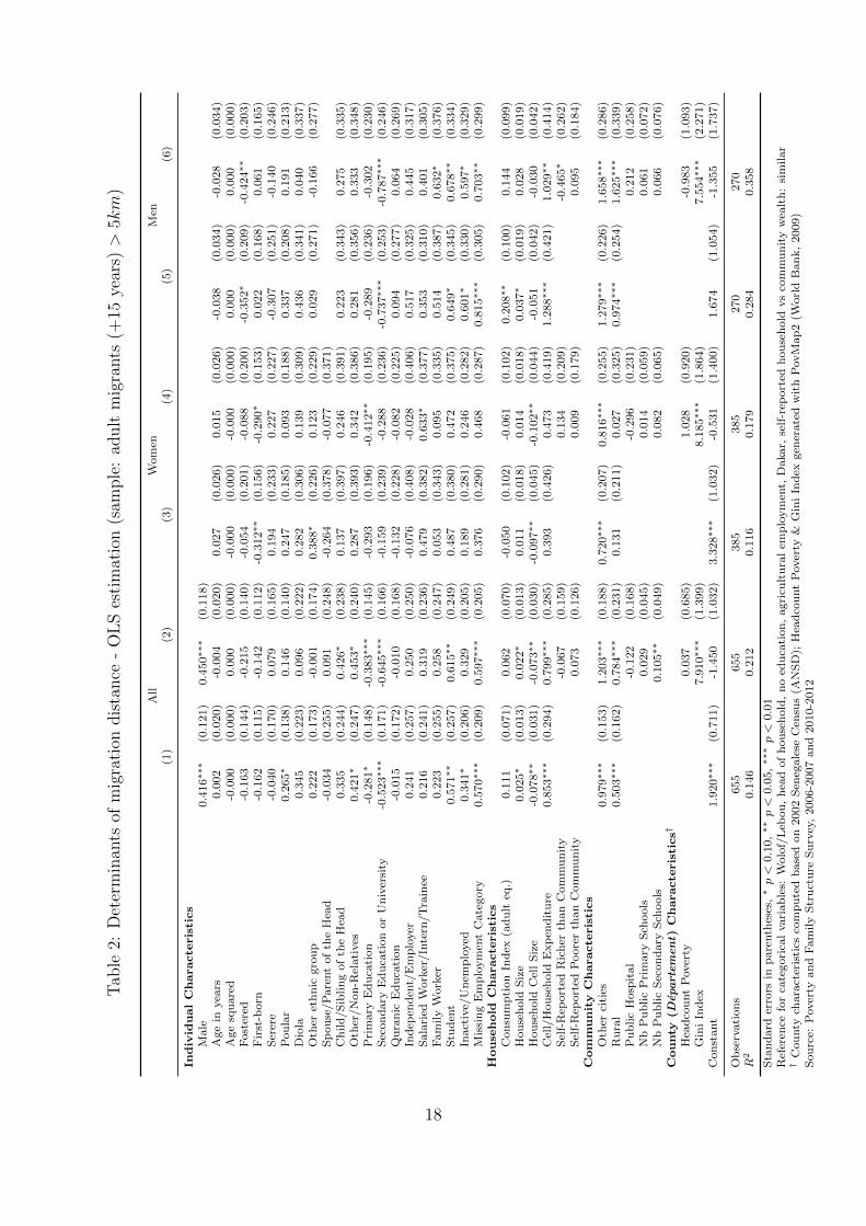
Having evaluated selection into migration, another crucial element of this analysis and

the originality of this paper is to evaluate the determinants of migration across distance.

Table 2 shows the results of OLS regressions using the logarithm of distance as dependent

variable, on the sample of internal migrants, i.e. individuals who moved of more than

5km, and separately for female and male migrants. Table 8, in Appendix, presents a

similar analysis but excludes intra-Dakar migrants, regardless of distance travelled, from

the regression samples.

Table 2 confirms the gendered nature of migration patterns as the distance travelled by

men is around 45% greater than that travelled by women. Separate regressions by gender

reveal different determinants of migration distance for men and women. Women are found

to migrate less far when they are the eldest of their siblings, consistent with gender roles in

the Senegalese society. Indeed, eldest daughters have an important parental role for their

youngest siblings. In addition, since marriage in Senegal is accompanied by a bridewealth

payment to the wife’s family, the marriage of the eldest daughter is expected to provide

their younger brothers with the resources to get married. This financial dependency of

the household on the marriage of the eldest daughter which is common to many other

African societies (Trinitapoli, Yeatman, and Fledderjohann, 2014; Horne, Dodoo, and

Dodoo, 2013) may explain in part that eldest daughters move less far, as their household

of origin seeks to maintain close links with her.

As for men, we find a positive impact of household wealth proxied by consumption

per adult equivalent on migration distance which is robust to the exclusion of intra-Dakar

migration. This result is consistent with the existence of migration costs, but also with

education as one of the primary reason for male migration that implies moving to the

capital city of Dakar and that only richer household can afford. Men with secondary

or higher education are found to move less far, which is very likely explained by higher

educational levels in regions close to the capital city where employment opportunities are

concentrated.

A common feature of male and female migrations is the positive relationship between

19

inequality in the county of origin and distance travelled. This finding is in line with

the theoretical framework developed by Stark (1984) and with relative deprivation as a

driver of migration, as individuals living in areas with a higher income inequality may

move further to escape relative poverty. Such result is also linked to the geography

of Senegal and the attractiveness of Dakar. As illustrated by Figure 1 , a majority

of individual trajectories converge from all regions towards Dakar. Moreover, the most

remote regions in the South-East of the country are also characterized by the largest levels

of inequality. By contrast, poverty at the county level is not significantly correlated with

migration distance. However, the coefficient on the poverty headcount becomes significant

for women only, when excluding intra-Dakar migrants (see Table 8, column 4). Note that

the negative effect of Dakar location (as opposed to rural and other urban areas) on

migration distance is fully explained by intra-Dakar migration, as the effect vanishes and

even reverses for women when excluding intra-Dakar relocation.

4.3 Rural-urban migration patterns

20

Tab

le3:

Mult

inom

ial

Log

itm

odel

sof

rura

l/urb

anm

igra

tion

dec

isio

n(m

argi

nal

effec

ts)

(1)

(2)

(3)

All

Wom

enM

enU

rban

Des

t.R

ura

lD

est.

Urb

an

Des

t.R

ura

lD

est.

Urb

an

Des

t.R

ura

lD

est.

Individ

ualCharacte

ristics

Male

-0.0

10

(0.0

07)

-0.0

17∗∗∗

(0.0

05)

Age

inyea

rs-0

.001

(0.0

01)

0.0

00

(0.0

01)

-0.0

02∗

(0.0

01)

0.0

01

(0.0

01)

0.0

01

(0.0

02)

-0.0

00

(0.0

01)

Age

squ

are

d0.0

00

(0.0

00)

-0.0

00

(0.0

00)

0.0

00

(0.0

00)

-0.0

00

(0.0

00)

-0.0

00

(0.0

00)

-0.0

00

(0.0

00)

Fost

ered

0.0

07

(0.0

08)

0.0

12∗∗

(0.0

05)

-0.0

05

(0.0

12)

0.0

20∗∗

(0.0

08)

0.0

18

(0.0

12)

0.0

04

(0.0

07)

Fir

st-b

orn

0.0

00

(0.0

06)

0.0

06

(0.0

04)

0.0

04

(0.0

09)

0.0

12∗

(0.0

06)

-0.0

05

(0.0

10)

-0.0

01

(0.0

05)

Born

inD

akar

-0.0

63∗∗∗

(0.0

10)

-0.0

19∗

(0.0

11)

-0.0

64∗∗∗

(0.0

14)

-0.0

23

(0.0

15)

-0.0

62∗∗∗

(0.0

16)

-0.0

13

(0.0

13)

Born

inru

ral

are

a-0

.026∗∗∗

(0.0

10)

0.0

47∗∗∗

(0.0

08)

-0.0

26∗∗

(0.0

13)

0.0

57∗∗∗

(0.0

12)

-0.0

30∗∗

(0.0

15)

0.0

31∗∗∗

(0.0

10)

Born

inoth

erco

untr

y-0

.017

(0.0

20)

0.0

21

(0.0

15)

-0.0

10

(0.0

23)

0.0

27

(0.0

22)

-0.0

26

(0.0

38)

0.0

15

(0.0

22)

Ser

ere

0.0

16∗

(0.0

09)

-0.0

08

(0.0

07)

0.0

24∗

(0.0

12)

-0.0

15

(0.0

10)

0.0

07

(0.0

13)

0.0

07

(0.0

09)

Pou

lar

-0.0

05

(0.0

08)

-0.0

00

(0.0

05)

0.0

05

(0.0

11)

-0.0

04

(0.0

08)

-0.0

18

(0.0

12)

0.0

08

(0.0

07)

Dio

la0.0

23∗

(0.0

12)

0.0

06

(0.0

10)

0.0

54∗∗∗

(0.0

15)

-0.0

22

(0.0

20)

-0.0

15

(0.0

21)

0.0

26∗∗

(0.0

10)

Oth

eret

hn

icgro

up

-0.0

01

(0.0

10)

0.0

08

(0.0

06)

0.0

12

(0.0

13)

0.0

05

(0.0

09)

-0.0

18

(0.0

16)

0.0

12

(0.0

08)

Sp

ou

se/P

are

nt

of

the

Hea

d-0

.014

(0.0

13)

0.0

02

(0.0

11)

-0.0

28

(0.0

17)

0.0

18

(0.0

24)

-0.6

45

(23.4

31)

-0.1

72

(12.6

50)

Ch

ild

/S

iblin

gof

the

Hea

d0.0

39∗∗∗

(0.0

12)

0.0

31∗∗∗

(0.0

11)

0.0

19

(0.0

19)

0.0

63∗∗∗

(0.0

24)

0.0

48∗∗∗

(0.0

17)

0.0

16

(0.0

11)

Oth

er/N

on

-Rel

ati

ves

0.0

43∗∗∗

(0.0

12)

0.0

30∗∗∗

(0.0

11)

0.0

13

(0.0

19)

0.0

44∗

(0.0

24)

0.0

71∗∗∗

(0.0

18)

0.0

36∗∗∗

(0.0

11)

Pri

mary

Ed

uca

tion

0.0

30∗∗∗

(0.0

09)

-0.0

11∗

(0.0

06)

0.0

20∗

(0.0

11)

-0.0

19∗∗

(0.0

09)

0.0

40∗∗∗

(0.0

14)

0.0

01

(0.0

08)

Sec

on

dary

Ed

uca

tion

or

Un

iver

sity

0.0

42∗∗∗

(0.0

10)

-0.0

08

(0.0

08)

0.0

40∗∗∗

(0.0

13)

-0.0

43∗∗∗

(0.0

17)

0.0

51∗∗∗

(0.0

15)

0.0

08

(0.0

08)

Qu

ran

icE

du

cati

on

-0.0

01

(0.0

10)

-0.0

04

(0.0

05)

-0.0

07

(0.0

15)

-0.0

00

(0.0

08)

0.0

00

(0.0

16)

-0.0

06

(0.0

08)

Ind

epen

den

t/E

mp

loyer

0.0

33∗∗

(0.0

15)

-0.0

24∗∗

(0.0

11)

0.0

24

(0.0

22)

-0.0

48∗∗

(0.0

21)

0.0

37∗

(0.0

19)

-0.0

10

(0.0

11)

Sala

ried

Work

er/In

tern

/T

rain

ee0.0

33∗∗

(0.0

14)

-0.0

10

(0.0

09)

0.0

17

(0.0

23)

-0.0

19

(0.0

17)

0.0

42∗∗

(0.0

19)

-0.0

08

(0.0

10)

Fam

ily

Work

er0.0

09

(0.0

17)

0.0

05

(0.0

07)

0.0

10

(0.0

24)

0.0

09

(0.0

11)

0.0

10

(0.0

24)

-0.0

05

(0.0

10)

Stu

den

t0.0

43∗∗∗

(0.0

16)

0.0

03

(0.0

10)

0.0

38∗

(0.0

23)

0.0

09

(0.0

18)

0.0

44∗∗

(0.0

22)

0.0

01

(0.0

10)

Inact

ive/

Un

emp

loyed

0.0

30∗∗

(0.0

13)

-0.0

04

(0.0

07)

0.0

32∗

(0.0

19)

-0.0

02

(0.0

10)

0.0

34∗

(0.0

20)

-0.0

16

(0.0

12)

Mis

sin

gE

mp

loym

ent

cate

gory

0.0

38∗∗∗

(0.0

13)

0.0

04

(0.0

07)

0.0

51∗∗∗

(0.0

19)

0.0

05

(0.0

10)

0.0

22

(0.0

18)

-0.0

02

(0.0

08)

House

hold

Characte

ristics

Con

sum

pti

on

Ind

ex(a

du

lteq

.)0.0

12∗∗∗

(0.0

04)

-0.0

00

(0.0

03)

0.0

10∗

(0.0

05)

-0.0

02

(0.0

04)

0.0

14∗∗

(0.0

06)

0.0

01

(0.0

04)

Hou

seh

old

Siz

e-0

.001

(0.0

01)

-0.0

01

(0.0

00)

-0.0

01

(0.0

01)

-0.0

01

(0.0

01)

-0.0

01

(0.0

01)

-0.0

00

(0.0

01)

Hou

seh

old

Cel

lS

ize

-0.0

03∗

(0.0

02)

0.0

02∗

(0.0

01)

-0.0

03

(0.0

02)

0.0

03∗

(0.0

02)

-0.0

03

(0.0

03)

0.0

01

(0.0

01)

Cel

l/H

ou

seh

old

Exp

end

itu

re0.0

29∗

(0.0

17)

-0.0

18

(0.0

13)

0.0

26

(0.0

23)

-0.0

19

(0.0

20)

0.0

31

(0.0

26)

-0.0

19

(0.0

17)

Sel

f-R

eport

edR

ich

erth

an

Com

mu

nit

y0.0

02

(0.0

09)

-0.0

03

(0.0

06)

0.0

08

(0.0

11)

0.0

06

(0.0

08)

-0.0

06

(0.0

14)

-0.0

23∗

(0.0

14)

Sel

f-R

eport

edP

oore

rth

an

Com

mu

nit

y0.0

16∗∗

(0.0

07)

-0.0

07

(0.0

05)

0.0

20∗∗

(0.0

09)

-0.0

13

(0.0

08)

0.0

08

(0.0

11)

0.0

00

(0.0

06)

Com

munity

Characte

ristics

Oth

erci

ties

-0.0

46∗∗∗

(0.0

12)

-0.0

45∗∗∗

(0.0

09)

-0.0

55∗∗∗

(0.0

15)

-0.0

66∗∗∗

(0.0

14)

-0.0

38∗∗

(0.0

18)

-0.0

20∗

(0.0

11)

Ru

ral

-0.0

08

(0.0

15)

-0.0

70∗∗∗

(0.0

11)

-0.0

24

(0.0

20)

-0.0

91∗∗∗

(0.0

17)

0.0

19

(0.0

23)

-0.0

36∗∗∗

(0.0

14)

Pu

blic

Hosp

ital

0.0

01

(0.0

09)

-0.0

07

(0.0

06)

0.0

18

(0.0

11)

-0.0

07

(0.0

10)

-0.0

21

(0.0

13)

-0.0

04

(0.0

08)

Nb

Pu

blic

Pri

mary

Sch

ools

-0.0

01

(0.0

02)

-0.0

02

(0.0

02)

-0.0

00

(0.0

03)

-0.0

02

(0.0

03)

-0.0

02

(0.0

04)

-0.0

05∗

(0.0

03)

Nb

Pu

blic

Sec

on

dary

Sch

ools

-0.0

02

(0.0

03)

-0.0

03

(0.0

02)

-0.0

03

(0.0

03)

-0.0

04

(0.0

03)

-0.0

00

(0.0

04)

-0.0

03

(0.0

03)

County

(Depart

em

en

t)Characte

ristics†

Hea

dco

unt

Pover

ty0.0

77∗

(0.0

41)

0.1

12∗∗∗

(0.0

29)

0.1

07∗∗

(0.0

54)

0.1

41∗∗∗

(0.0

44)

0.0

40

(0.0

62)

0.0

60

(0.0

37)

Gin

iIn

dex

-0.1

89∗∗

(0.0

83)

-0.0

54

(0.0

53)

-0.1

54

(0.1

06)

-0.0

64

(0.0

76)

-0.2

45∗

(0.1

30)

-0.0

46

(0.0

70)

Ob

serv

ati

on

s6906

6906

3842

3842

3064

3064

Sta

nd

ard

erro

rsin

pare

nth

eses

,∗p<

0.1

0,∗∗p<

0.0

5,∗∗∗p<

0.0

1R

efer

ence

for

cate

gori

cal

vari

ab

les:

Wolo

f/L

ebou

,h

ead

of

hou

seh

old

,n

oed

uca

tion

,agri

cult

ura

lem

plo

ym

ent,

Dakar,

self

-rep

ort

edh

ou

seh

old

vs

com

mu

nit

yw

ealt

h:

sim

ilar

†C

ou

nty

chara

cter

isti

csco

mp

ute

db

ase

don

2002

Sen

egale

seC

ensu

s(A

NS

D);

Hea

dco

unt

Pover

ty&

Gin

iIn

dex

gen

erate

dw

ith

PovM

ap

2(W

orl

dB

an

k,

2009)

Sou

rce:

Pover

tyan

dF

am

ily

Str

uct

ure

Su

rvey

,2006-2

007

an

d2010-2

012

21

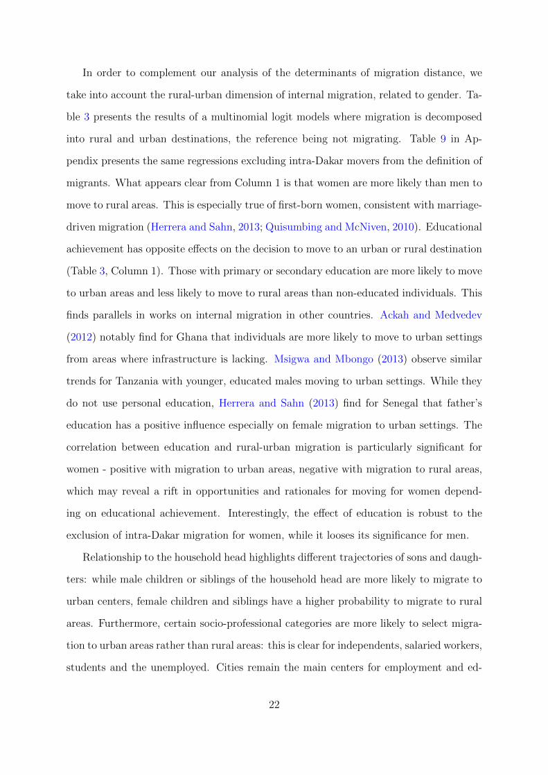
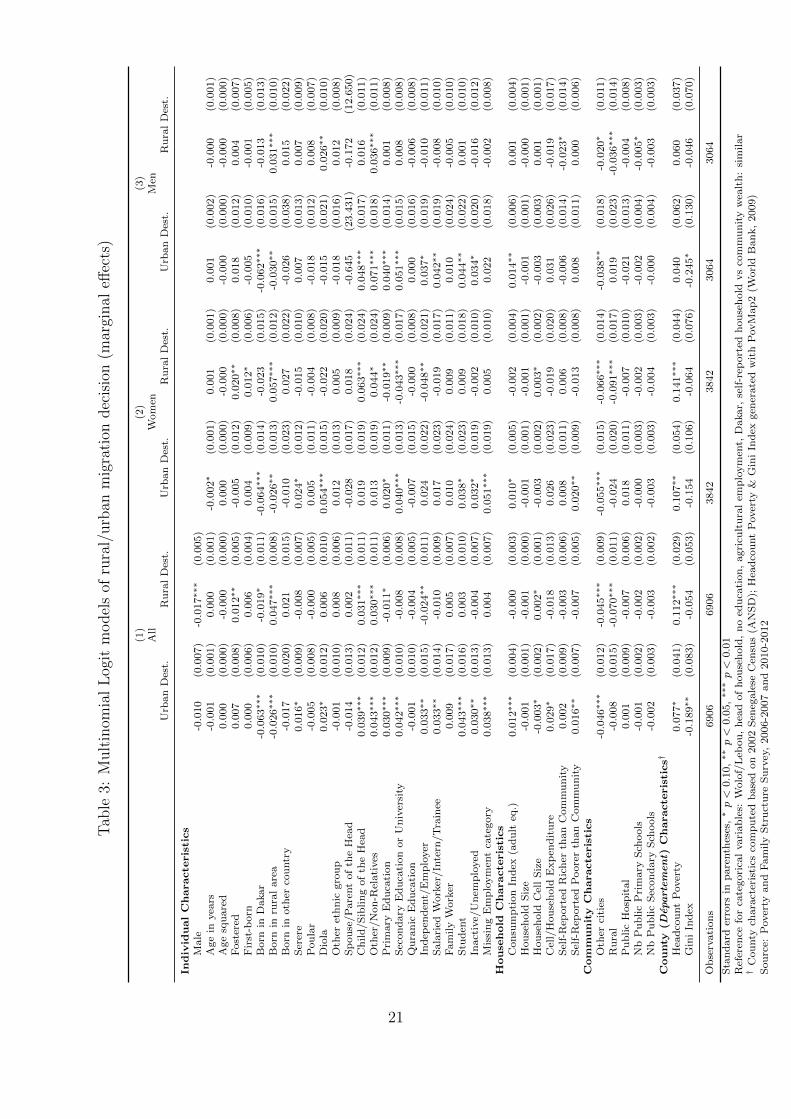
In order to complement our analysis of the determinants of migration distance, we

take into account the rural-urban dimension of internal migration, related to gender. Ta-

ble 3 presents the results of a multinomial logit models where migration is decomposed

into rural and urban destinations, the reference being not migrating. Table 9 in Ap-

pendix presents the same regressions excluding intra-Dakar movers from the definition of

migrants. What appears clear from Column 1 is that women are more likely than men to

move to rural areas. This is especially true of first-born women, consistent with marriage-

driven migration (Herrera and Sahn, 2013; Quisumbing and McNiven, 2010). Educational

achievement has opposite effects on the decision to move to an urban or rural destination

(Table 3, Column 1). Those with primary or secondary education are more likely to move

to urban areas and less likely to move to rural areas than non-educated individuals. This

finds parallels in works on internal migration in other countries. Ackah and Medvedev

(2012) notably find for Ghana that individuals are more likely to move to urban settings

from areas where infrastructure is lacking. Msigwa and Mbongo (2013) observe similar

trends for Tanzania with younger, educated males moving to urban settings. While they

do not use personal education, Herrera and Sahn (2013) find for Senegal that father’s

education has a positive influence especially on female migration to urban settings. The

correlation between education and rural-urban migration is particularly significant for

women - positive with migration to urban areas, negative with migration to rural areas,

which may reveal a rift in opportunities and rationales for moving for women depend-

ing on educational achievement. Interestingly, the effect of education is robust to the

exclusion of intra-Dakar migration for women, while it looses its significance for men.

Relationship to the household head highlights different trajectories of sons and daugh-

ters: while male children or siblings of the household head are more likely to migrate to

urban centers, female children and siblings have a higher probability to migrate to rural

areas. Furthermore, certain socio-professional categories are more likely to select migra-

tion to urban areas rather than rural areas: this is clear for independents, salaried workers,

students and the unemployed. Cities remain the main centers for employment and ed-

22

ucation (Beauchemin and Bocquier, 2004). Unsurprisingly, individuals from wealthier

households tend to migrate to urban areas. Interestingly, subjective relative household

wealth is related in a different way to male and female migration. Men in self-perceived

richer households have a lower probability to move to rural areas, while women in rel-

atively poor households are more likely to migrate to urban settings. Our results for

women are consistent with relative deprivation as a driver of migration decisions, but

such an assumption is not supported by empirical evidence for men. The effect of indices

measured at the county level confirm that higher poverty rate increase female migration

to both destinations.

Excluding intra-Dakar mobility, we find that being born in a rural area has a positive

effect on the probability of migrating to a rural area which is found significant for women

only (Table 9, column 4). Additional specifications decomposing migration by both des-

tination and origin provide consistent evidence that women are more likely to experience

rural-to-rural moves than men (results not shown, available upon request).

4.4 Treatment of attrition

A crucial issue when studying migration using panel data is linked to attrition. Individu-

als who were not found in the second survey wave are presumably in large part individuals

who left their household of origin, and maybe moved far away enough that surveyors were

not able to find them in their community of origin. It could thus be argued that attritors

should be treated as migrants. However, as we focus on internal migration such a solu-

tion tends to overinflate both the importance of internal migration and the consequences

of attrition. Indeed, a non-negligible share of attritors is expected to fall outside the

scope of our analysis: first, whereas it seems doubtless that individuals who could not be

found in their household of origin have moved, some are likely to have migrated abroad.

Second, even when excluding international migrants, attritors do not exactly match our

definition of migrants, as we consider a lower bound of 5km as the minimum distance

associated with mobility costs high enough to discriminate migration from mere housing

23

mobility. Indeed, a significant share of attritors may have moved relatively close to their

household of origin and still be lost, especially in Dakar. Note that 57% of attrition

concerns individuals living in Dakar, where individuals may not be as easily traced as

in smaller towns or rural communities. Furthermore we observe a high mobility within

Dakar, which supports our assumption that among attritors who were still alive and re-

mained in Senegal, a non negligible share falls out of our definition of internal migrants.

Tables 10 and 11 in Appendix compare the observed characteristics of attritors to those of

four distinct groups: internal migrants (i.e. individuals who moved of more than 5km),

deceased individuals, international migrants and movers of less than 5km. Columns 6

to 9 test the equality of the mean or percentages for the different variables used in the

analysis. The tests suggest that attritors have characteristics which are closer on average

to those of international migrants than to any other group. This is particularly true with

regard to education, socio-professional category, household measured and self-perceived

wealth, and community infrastructures, for which no significant difference is observed be-

tween individuals who could not be tracked and international migrants. This observation,

although it cannot be used as a proof, suggests that international migration is probably

a major driver of attrition.

In order to analyze the sensitivity of our results to attrition, we estimated a probit

model for internal migration treating attritors as internal migrants. For the above stated

reasons, considering individuals who could not be tracked as internal migrants leads us

to overinflate the internal migrant category, since, as discussed above, attrition is also

probably caused in part by death, international migration and short-distance housing

mobility. Results are presented in Table 12, columns 1 to 3 for the total sample, and

separately for women and men, together with the results of probit models for the determi-

nants of attrition. First, the coefficient on the male dummy in column 1 is not significant

when treating attrition as internal migration. Indeed, men are more likely than women

to be lost between the two survey rounds. This finding confirms that female migration

is less independent than male migration, as women are more easily tracked, meaning

24

that they may be less likely to cut-off links with their origin household when moving. In

addition, the share of attrition due to the loss of the entire household is lower for women

(45.9%) than for men (52.3%). The difference is partly due to the frequent loss of urban

one-person households characterized by a higher mobility and a lower insertion in local

networks. One-person households lost are almost exclusively male as women living alone

is a very marginal phenomenon: 43 male individuals living alone were lost, representing

15.2% of male attrition, compared to 6 women only (2.6% of female attrition). However,

apart from the different gender composition of the attrited and migrant population, most

observations driven from Table 1 are unchallenged when treating attrition as internal

migration. When looking more specifically at the determinants of attrition, we find that

individuals with low levels of education, weak ties to the head of the household and

living in Dakar are more likely to have been lost. For women, attrition is very likely

driven in part by the high mobility of young salaried domestic workers (maids or petites

bonnes), documented in the Malian case by Lesclingand (2011). Such an interpretation

is supported by the positive and significant coefficient on the salaried worker dummy in

the female regression (column 5) and the positive correlation with household income as

only relatively wealthy households can afford to employ domestic workers. By contrast,

male attrition may be caused in part by international migration, as male spouses of the

head are more likely to be lost, as well as individuals from wealthier households. This

result is consistent with the descriptive statistics showing that attritors and international

migrants share many common features (10 and 11). In sum, although male attrition is

more frequently observed, it may have little impact on our analysis, as it seems to be

driven in part by international migration. On the other hand, female attrition is less

frequent but seems to be specific to vulnerable populations with low-level and precarious

jobs. Our study probably misses part of the phenomenon of female migration by losing

track of these highly mobile urban populations living at the periphery of their household.

However, to mitigate this issue, it is important to note that such mobility could be called

secondary in the sense that in order to get employed, these women had already migrated

25

from their household of origin with which they may have kept links. The primary mobility

of this specific population should thus appear in our data.

Attrition may also be an issue for the analysis of migration distance. Indeed, as attri-

tion is partly caused by internal migration, it may be correlated with migration distance.

The sign of the correlation is however ambiguous: individuals migrating further away

may be less easily tracked, but short-distance urban mobility may generate more attri-

tion due to the weaker neighbourhood networks. Our estimates of the determinants of

migration distance may thus be biased by selective attrition. However, the distance trav-

elled by those among attritors who are indeed internal migrants is unknown. The above

robustness checks consisting in pooling attritors and internal migrants in the analysis of

the probability of migrating is not applicable for migration distance. In order to investi-

gate this issue we thus choose another approach. Following Senne (2014), we estimate a

two-step Heckman (1979) selection model, using dummies for second-wave fieldwork con-

troller in charge of first recontacting households at their first-wave location as excluded

instruments8. Indeed, the success of the tracking of individuals who had left their initial

household heavily relied on the accuracy of information collected among other household

members found at first-wave location of the household, or among neighbours if the whole

household had moved. We expect individual characteristics of fieldwork controllers to

have an impact on tracking outcomes, and thus on attrition, while being uncorrelated

with migration distance. Second-stage estimates are reported in Table 13 in Appendix.

The comparison of results shown in Tables 2 and 13 suggests that the bias due to attrition

is small, as the sign, size and significance of coefficients in both tables are very close.

8Ten teams of two to three surveyors were managed on the field by one controller each, who wasin particular in charge of checking compliance with procedures and of verifying that accurate trackinginformation had been reported by surveyors.

26

5 Conclusion

This article studies the determinants of internal migration using rich individual panel

survey data collected in Senegal in 2006-07 and 2010-12. The tracking of all individuals

who remained in Senegal allow us to identify and map migrations between the two survey

waves using the GPS coordinates at both dates. These features of our data are unique in

this region of the world and allow us to make a significant contribution to the literature

on internal migration in sub-Saharan Africa. Using distance rather than administrative

boundaries has the advantage of providing us with a definition of migration which is less

arbitrary and homogeneous across regions.

The empirical analysis reveals clear differences between women and men. Women are

more likely than men to have migrated between the two survey rounds, however, they

tend to migrate over shorter distances. The decomposition of the migration decision

in rural and urban destinations confirms and complements this study by showing that

women are more likely than men to migrate to rural areas, especially when originating

from rural areas. Such moves are related to the different motivations behind male and

female migration. The primary reason for migrating for women in our sample is marriage,

whatever the distance travelled. By contrast, labor and education are the most cited

motives behind male migration.

Our findings reveal surprisingly little change since the pioneering works on female

migration dating back from the early 1990s (Chant et al., 1992). Female migration still

depends in a large part on family events and has few connections with labor market

participation, contrary to male migration. For this reason, women are over-represented

in rural-to-rural flows while rural-to-urban migration is more commonly observed for men.

These observations echo the conclusions of De Brauw, Mueller, and Lee (2014) noting

the surprisingly low rural-urban flows in sub-Saharan Africa given the rural-income wage

gap. In the light of our results, policies aimed at encouraging rural to urban migration

that would target women would presumably have a stronger impact, as women are still

27

largely marginalized from labor-related moves. In line with De Brauw, Mueller, and Lee

(2014), the present study shows that education increases the likelihood of migrating to

urban areas especially for women, suggesting an efficient channel for promoting women’s

access to independent migration.

28

References

Ackah, Charles and Denis Medvedev. 2012. “Internal migration in Ghana: determinants

and welfare impacts.” International Journal of Social Economics 39 (10):764–784.

ANSD (Agence Nationale de la Statistique et de la Demographie). 2006. RGPH III – Rap-

port national de presentation des resultats definitifs. Resultats definitifs du troisieme

recensement general de la population et de l’habitat, 2002. ANSD, Dakar, Senegal.

Assaad, Ragui and Melanie Arntz. 2005. “Constrained geographical mobility and gen-

dered labor market outcomes under structural adjustment: Evidence from Egypt.”

World Development 33 (3):431–454.

Beauchemin, Cris. 2011. “Rural–urban migration in West Africa: towards a reversal? Mi-

gration trends and economic situation in Burkina Faso and Cote d’Ivoire.” Population,

Space and Place 17 (1):47–72.

Beauchemin, Cris and Philippe Bocquier. 2004. “Migration and urbanisation in Fran-

cophone West Africa: An overview of the recent empirical evidence.” Urban Studies

41 (11):2245–2272.

Beck, Simon, Philippe De Vreyer, Sylvie Lambert, Karine Marazyan, Abla Safir et al.

2011. “Child fostering in Senegal.”

Bell, Martin, Marcus Blake, Paul Boyle, Oliver Duke-Williams, Philip Rees, John Still-

well, and Graeme Hugo. 2002. “Cross-national comparison of internal migration: issues

and measures.” Journal of the Royal Statistical Society: Series A (Statistics in Society)

165 (3):435–464.

Bell, Martin, Elin Charles-Edwards, Dorota Kupiszewska, Marek Kupiszewski, John Still-

well, and Yu Zhu. 2015. “Internal migration data around the world: Assessing contem-

porary practice.” Population, Space and Place 21 (1):1–17.

29

Bocquier, Philippe and Andrew Kabulu Mukandila. 2013. “African urbanization trends

and prospects.” .

Brockerhoff, Martin and Hongsook Eu. 1993. “Demographic and socioeconomic deter-

minants of female rural to urban migration in Sub-Saharan Africa.” International

Migration Review :557–577.

Chant, Sylvia et al. 1992. Gender & migration in developing countries. Belhaven Press.

Chort, Isabelle. 2014. “Mexican Migrants to the US: What Do Unrealized Migration

Intentions Tell Us About Gender Inequalities?” World development 59:535–552.

Chort, Isabelle and Jean-Noel Senne. 2015. “Selection into Migration within a Household

Model: Evidence from Senegal.” The World Bank Economic Review 29 (suppl 1):S247–

S256.

Clark, William and Youqin Huang. 2004. “Linking migration and mobility: individual

and contextual effects in housing markets in the UK.” Regional studies 38 (6):617–628.

Cordey-Hayes, M and D Gleave. 1974. “Migration movements and the differential growth

of city regions in England and Wales.” Papers in Regional Science 33 (1):99–123.

De Brauw, Alan, Valerie Mueller, and Hak Lim Lee. 2014. “The role of rural–urban

migration in the structural transformation of Sub-Saharan Africa.” World Development

63:33–42.

DeVreyer, Philippe, Sylvie Lambert, Abla Safir, and Momar Sylla. 2008. “Pauvrete et

Structure Familiale: Pourquoi une nouvelle enquete ?” Stateco 102.

Dustmann, Christian and Anna Okatenko. 2014. “Out-migration, wealth constraints, and

the quality of local amenities.” Journal of Development Economics 110:52–63.

Elbers, Chris, Jean O Lanjouw, and Peter Lanjouw. 2003. “Micro–level estimation of

poverty and inequality.” Econometrica 71 (1):355–364.

30

Heckman, James. 1979. “Sample Selection Bias as a Specification Error.” Econometrica

.

Herrera, Catalina and David E Sahn. 2013. “Determinants of Internal Migration among

Senegalese Youth.” Cornell Food and Nutrition Policy Program Working Paper 245.

Horne, Christine, F Nii-Amoo Dodoo, and Naa Dodua Dodoo. 2013. “The shadow of

indebtedness: Bridewealth and norms constraining female reproductive autonomy.”

American Sociological Review :0003122413484923.

Kanaiaupuni, Shawn Malia. 2000. “Reframing the migration question: An analysis of

men, women, and gender in Mexico.” Social forces 78 (4):1311–1347.

Kudo, Yuya. 2015. “Female migration for marriage: Implications from the land reform

in rural Tanzania.” World Development 65:41–61.

Lambert, Sylvie, Martin Ravallion, and Dominique van de Walle. 2014. “Intergenerational

mobility and interpersonal inequality in an African economy.” Journal of Development

Economics 110:327 – 344.

Lesclingand, Marie. 2011. “Migrations des jeunes filles au Mali: exploitation ou

emancipation?” Travail, genre et societes (1):23–40.

Massey, Douglas S, Mary J Fischer, and Chiara Capoferro. 2006. “International migra-

tion and gender in Latin America: A comparative analysis.” International Migration

44 (5):63–91.

Msigwa, Robert Ebihart and James Ezekiel Mbongo. 2013. “Determinants of internal

migration in Tanzania.” Journal of Economics and Sustainable Development 4 (9):28–

35.

Niedomysl, Thomas and Urban Fransson. 2014. “On distance and the spatial dimen-

sion in the definition of internal migration.” Annals of the Association of American

Geographers 104 (2):357–372.

31

Potts, Deborah. 2009. “The slowing of sub-Saharan Africa’s urbanization: evidence and

implications for urban livelihoods.” Environment and Urbanization 21 (1):253–259.

———. 2012. “Challenging the myths of urban dynamics in sub-Saharan Africa: The

evidence from Nigeria.” World Development 40 (7):1382–1393.

Quisumbing, Agnes and Scott McNiven. 2010. “Moving forward, looking back: The

impact of migration and remittances on assets, consumption, and credit constraints in

the rural Philippines.” The Journal of Development Studies 46 (1):91–113.

Rosenzweig, Mark R and Oded Stark. 1989. “Consumption smoothing, migration, and

marriage: Evidence from rural India.” The Journal of Political Economy :905–926.

Senne, Jean-Noel. 2014. “Death and schooling decisions over the short and long run in

rural Madagascar.” Journal of Population Economics 27 (2):497–528.

Stark, Oded. 1984. “Rural-to-urban migration in LDCs: a relative deprivation approach.”

Economic Development and Cultural Change 32 (3):475–486.

Stark, Oded and David E Bloom. 1985. “The new economics of labor migration.” The

american Economic review 75 (2):173–178.

Stark, Oded and J Edward Taylor. 1989. “Relative deprivation and international migra-

tion oded stark.” Demography 26 (1):1–14.

Thadani, Veena N and Michael P Todaro. 1984. “Female migration: a conceptual frame-

work.” .

Todaro, Michael P. 1997. “Urbanization unemployment and migration in Africa: theory

and policy.” .

Trinitapoli, Jenny, Sara Yeatman, and Jasmine Fledderjohann. 2014. “Sibling support

and the educational prospects of young adults in Malawi.” Demographic research

30:547.

32

UNDP. 2009. Overcoming Barriers: Human Mobility and Development. Palgrave Macmil-

lan.

Zhao, Qinghua and Peter Lanjouw. 2009. “Using PovMap2-A User’s Guide.” The World

Bank .

33

Appendix

34

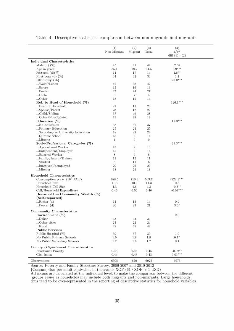
Table 4: Descriptive statistics: comparison between non-migrants and migrants

(1) (2) (3) (4)Non-Migrant Migrant Total t/χ2

diff (1) - (2)

Individual CharacteristicsMale (d) (%) 45 41 44 2.68Age in years 35.1 28.2 34.5 6.9∗∗∗

Fostered (d)(%) 14 17 14 4.6∗∗

First-born (d) (%) 34 32 33 1.1Ethnicity (%) 20.0∗∗∗

...Wolof/Lebou 42 38 42

...Serere 12 16 13

...Poular 27 24 27

...Diola 5 7 5

...Other 13 15 14Rel. to Head of Household (%) 126.1∗∗∗

...Head of Household 21 11 20

...Spouse/Parent 23 12 22

...Child/Sibling 37 49 38

...Other/Non-Related 19 29 19Education (%) 17.3∗∗∗

...No Education 38 37 37

...Primary Education 25 24 25

...Secondary or University Education 18 29 24

...Quranic School 18 9 14

...Missing 1 0 0Socio-Professional Categories (%) 64.3∗∗∗

...Agricultural Worker 13 9 13

...Independent/Employer 15 9 14

...Salaried Worker 8 9 8

...Family/Intern/Trainee 11 12 11

...Student 6 11 6

...Inactive/Unemployed 29 26 29

...Missing 18 24 18

Household CharacteristicsConsumption p.a.e. (103 XOF) 488.5 710.6 509.7 -222.1∗∗∗

Household Size 11.3 10.9 11.3 0.5Household Cell Size 4.3 4.6 4.3 -0.3∗∗

Cell/Household Expenditure 0.46 0.50 0.46 -0.04∗∗∗

Household vs Community Wealth (%)(Self-Reported)...Richer (d) 14 13 14 0.9...Poorer (d) 20 23 21 3.6∗

Community CharacteristicsEnvironment (%) 2.6...Dakar 33 33 33...Other cities 24 22 24...Rural 42 45 42Public ServicesPublic Hospital (%) 39 37 39 1.9Nb Public Primary Schools 1.9 1.8 1.9 0.1∗

Nb Public Secondary Schools 1.7 1.6 1.7 0.1

County (Departement CharacteristicsHeadcount Poverty 0.45 0.46 0.45 -0.02∗∗

Gini Index 0.44 0.43 0.43 0.01∗∗∗

Observations 6305 670 6975 6975

Source: Poverty and Family Structure Survey, 2006-2007 and 2010-2012†Consumption per adult equivalent in thousands XOF (619 XOF ≈ 1 USD)All means are calculated at the individual level, to make the comparison between the differentgroups easier as households may include both migrants and non-migrants. Large households

thus tend to be over-represented in the reporting of descriptive statistics for household variables.

35

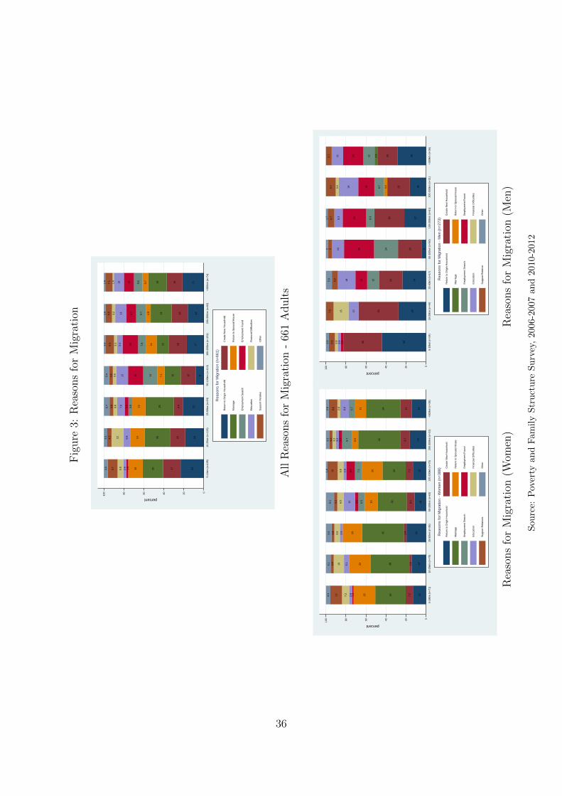
Fig

ure

3:R

easo

ns

for

Mig

rati

on

231720151.9

2.9

5.8

9.7

3.9

191525146.8

124.2

3.4

219.4

28133.8

3.8

7.5

3.8

3.8

5.7

815167.1

1415123.6

3.6

5.4

171812117.8

165.4

3.1

8.5

1.6

1616214.8

9.7

9.7

113.2

6.5

1.6

2116195.7

8.6

10101.4

7.1

1.4

020406080100

percent

5-10

km (

n=10

5)10

-25k

m (

n=12

3)25

-50k

m (

n=53

)50

-100

km (

n=11

3)10

0-20

0km

(n=

131)

200-

300k

m (

n=62

)+

300k

m (

n=74

)

Ret

urn

to O

rigin

Hou

seho

ldC

reat

e N

ew H

ouse

hold

Mar

riage

Ret

urn

to S

pous

al H

ouse

Em

ploy

men

t Sea

rch

Em

ploy

men

t Fou

nd

Edu

catio

nF

inan

cial

Diff

icul

ties

Sup

port

Rel

ativ

eO

ther

Rea

sons

for

Mig

ratio

n (n

=66

1)

All

Rea

sons

for

Mig

rati

on-

661

Adult

s

137.2

30221.4

2.9

7.2

124.3

142.6

38225.1

102.6

5.1

192.8

42192.8

5.6

2.8

5.6

118.1

29136.5

3.2

116.5

3.2

8.1

137.2

23207.2

8.7

2.9

5.8

101.4

169.7

426.5

9.7

3.2

3.2

3.2

3.2

3.2

141134115.7

8.6

2.9

8.6

2.9

020406080100

percent

5-10

km (

n=71

)10

-25k

m (

n=79

)25

-50k

m (

n=36

)50

-100

km (

n=63

)10

0-20

0km

(n=

70)

200-

300k

m (

n=31

)+

300k

m (

n=38

)

Ret

urn

to O

rigin

Hou

seho

ldC

reat

e N

ew H

ouse

hold

Mar

riage

Ret

urn

to S

pous

al H

ouse

Em

ploy

men

t Sea

rch

Em

ploy

men

t Fou

nd

Edu

catio

nF

inan

cial

Diff

icul

ties

Sup

port

Rel

ativ

esO

ther

Rea

sons

for

Mig

ratio

n -

Wom

en (

n=38

8)

Rea

sons

for

Mig

rati

on(W

omen

)

44382.9

2.9

2.9

5.9

2.9

284010157.5

24241212185.9

5.9

42424301242

22308.3

238.3

6.7

1.7

16233.2

9.7

16193.2

9.7

29202.9

1120115.7

020406080100

percent

5-10

km (

n=34

)10

-25k

m (

n=44

)25

-50k

m (

n=17

)50

-100

km (

n=50

)10

0-20

0km

(n=

61)

200-

300k

m (

n=31

)+

300k

m (

n=36

)

Ret

urn

to O

rigin

Hou

seho

ldC

reat

e N

ew H

ouse

hold

Mar

riage

Ret

urn

to S

pous

al H

ouse

Em

ploy

men

t Sea

rch

Em

ploy

men

t Fou

nd

Edu

catio

nF

inan

cial

Diff

icul

ties

Sup

port

Rel

ativ

eO

ther

Rea

sons

for

Mig

ratio

n -

Men

(n=

273)

Rea

sons

for

Mig

rati

on(M

en)

Sou

rce:

Pov

erty

an

dF

am

ily

Str

uct

ure

Su

rvey

,2006-2

007

and

2010-2

012

36

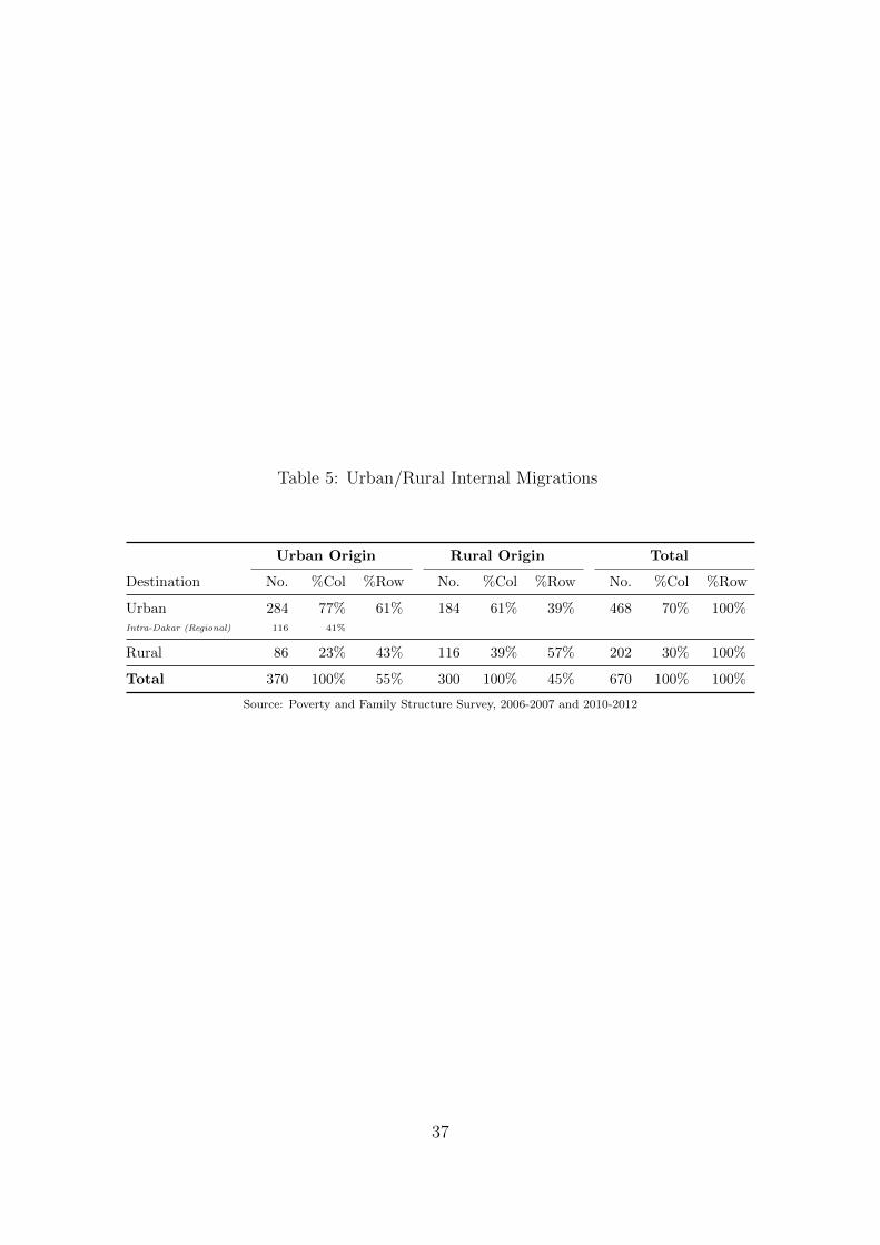
Table 5: Urban/Rural Internal Migrations

Urban Origin Rural Origin Total

Destination No. %Col %Row No. %Col %Row No. %Col %Row

Urban 284 77% 61% 184 61% 39% 468 70% 100%Intra-Dakar (Regional) 116 41%

Rural 86 23% 43% 116 39% 57% 202 30% 100%

Total 370 100% 55% 300 100% 45% 670 100% 100%

Source: Poverty and Family Structure Survey, 2006-2007 and 2010-2012

37

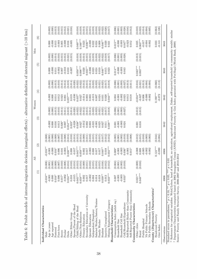
Tab

le6:

Pro

bit

model

sof

inte

rnal

mig

rati

ondec

isio

n(m

argi

nal

effec

ts)

-al

tern

ativ

edefi

nit

ion

ofin

tern

alm

igra

nt

(>10

km

)

All

Wom

enM

en(1

)(2

)(3

)(4

)(5

)(6

)

Individ

ualCharacte

ristics

Male

-0.0

16∗∗

(0.0

08)

-0.0

16∗∗

(0.0

08)

Age

inyea

rs-0

.001

(0.0

01)

-0.0

01

(0.0

01)

-0.0

02

(0.0

02)

-0.0

02

(0.0

02)

0.0

00

(0.0

02)

0.0

00

(0.0

02)

Age

squ

are

d0.0

00

(0.0

00)

-0.0

00

(0.0

00)

0.0

00

(0.0

00)

0.0

00

(0.0

00)

-0.0

00

(0.0

00)

-0.0

00

(0.0

00)

Fost

ered

0.0

16∗

(0.0

09)

0.0

16∗

(0.0

09)

0.0

16

(0.0

13)

0.0

14

(0.0

13)

0.0

14

(0.0

14)

0.0

13

(0.0

13)

Fir

st-b

orn

0.0

06

(0.0

07)

0.0

06

(0.0

07)

0.0

13

(0.0

10)

0.0

12

(0.0

10)

-0.0

02

(0.0

10)

-0.0

03

(0.0

10)

Ser

ere

0.0

17∗

(0.0

10)

0.0

16

(0.0

10)

0.0

26∗

(0.0

14)

0.0

23

(0.0

14)

0.0

07

(0.0

15)

0.0

05

(0.0

15)

Pou

lar

-0.0

02

(0.0

08)

-0.0

03

(0.0

08)

0.0

07

(0.0

11)

0.0

01

(0.0

12)

-0.0

10

(0.0

12)

-0.0

08

(0.0

12)

Dio

la0.0

34∗∗

(0.0

14)

0.0

38∗∗∗

(0.0

14)

0.0

54∗∗∗

(0.0

19)

0.0

57∗∗∗

(0.0

19)

0.0

10

(0.0

21)

0.0

16

(0.0

21)

Oth

erE

thn

icG

rou

p0.0

10

(0.0

10)

0.0

08

(0.0

10)

0.0

23∗

(0.0

14)

0.0

19

(0.0

14)

-0.0

07

(0.0

15)

-0.0

05

(0.0

16)

Sp

ou

se/P

are

nt

of

the

Hea

d-0

.015

(0.0

14)

-0.0

17

(0.0

14)

-0.0

28

(0.0

20)

-0.0

30

(0.0

20)

Ch

ild

/S

iblin

gof

the

Hea

d0.0

45∗∗∗

(0.0

13)

0.0

45∗∗∗

(0.0

13)

0.0

38∗

(0.0

22)

0.0

37∗

(0.0

22)

0.0

50∗∗∗

(0.0

18)

0.0

49∗∗∗

(0.0

18)

Oth

er/N

on

-Rel

ati

ves

0.0

59∗∗∗

(0.0

14)

0.0

59∗∗∗

(0.0

14)

0.0

27

(0.0

22)

0.0

27

(0.0

22)

0.0

98∗∗∗

(0.0

19)

0.1

00∗∗∗

(0.0

19)

Pri

mary

Ed

uca

tion

0.0

02

(0.0

09)

0.0

02

(0.0

09)

-0.0

12

(0.0

12)

-0.0

14

(0.0

12)

0.0

20

(0.0

14)

0.0

23

(0.0

14)

Sec

on

dary

Ed

uca

tion

or

Un

iver

sity

0.0

17

(0.0

11)

0.0

17

(0.0

11)

0.0

02

(0.0

15)

0.0

03

(0.0

15)

0.0

35∗∗

(0.0

15)

0.0

36∗∗

(0.0

15)

Qu

ran

icE

du

cati

on

-0.0

02

(0.0

10)

-0.0

03

(0.0

10)

0.0

03

(0.0

14)

0.0

03

(0.0

14)

-0.0

06

(0.0

15)

-0.0

08

(0.0

15)

Ind

epen

den

t/E

mp

loyer

0.0

04

(0.0

15)

0.0

08

(0.0

15)

-0.0

21

(0.0

23)

-0.0

15

(0.0

23)

0.0

23

(0.0

19)

0.0

22

(0.0

19)

Sala

ried

Work

er/In

tern

/T

rain

ee0.0

14

(0.0

14)

0.0

17

(0.0

14)

-0.0

01

(0.0

23)

0.0

07

(0.0

23)

0.0

24

(0.0

18)

0.0

24

(0.0

18)

Fam

ily

Work

er0.0

19

(0.0

15)

0.0

17

(0.0

15)

0.0

25

(0.0

21)

0.0

24

(0.0

21)

0.0

10

(0.0

22)

0.0

09

(0.0

22)

Stu

den

t0.0

39∗∗

(0.0

16)

0.0

40∗∗

(0.0

17)

0.0

27

(0.0

25)

0.0

31

(0.0

25)

0.0

46∗∗

(0.0

22)

0.0

46∗∗

(0.0

22)

Inact

ive/

Unem

plo

yed

0.0

13

(0.0

12)

0.0

18

(0.0

12)

0.0

11

(0.0

17)

0.0

20

(0.0

17)

0.0

15

(0.0

19)

0.0

20

(0.0

20)

Mis

sin

gE

mp

loym

ent

Cate

gory

0.0

33∗∗∗

(0.0

12)

0.0

34∗∗∗

(0.0

12)

0.0

38∗∗

(0.0

18)

0.0

44∗∗

(0.0

18)

0.0

23

(0.0

17)

0.0

21

(0.0

17)

House

hold

Characte

ristics

Con

sum

pti

on

Ind

ex(a

du

lteq

.)0.0

07

(0.0

04)

0.0

09∗

(0.0

05)

0.0

01

(0.0

06)

0.0

04

(0.0

06)

0.0

14∗∗

(0.0

06)

0.0

15∗∗

(0.0

06)

Hou

seh

old

Siz

e-0

.001

(0.0

01)

-0.0

01

(0.0

01)

-0.0

01

(0.0

01)

-0.0

01

(0.0

01)

-0.0

00

(0.0

01)

-0.0

00

(0.0

01)

Hou

seh

old

Cel

lS

ize

-0.0

03

(0.0

02)

-0.0

03

(0.0

02)

-0.0

03

(0.0

03)

-0.0

02

(0.0

03)

-0.0

03

(0.0

03)

-0.0

03

(0.0

03)

Cel

l/H

ou

seh

old

Exp

end

itu

re0.0

33∗

(0.0

19)

0.0

36∗

(0.0

19)

0.0

24

(0.0

27)

0.0

23

(0.0

27)

0.0

43

(0.0

28)

0.0

47∗

(0.0

28)

Sel

f-R

eport

edR

ich

erth

an

Com

mu

nit

y-0

.001

(0.0

10)

0.0

13

(0.0

13)

-0.0

23

(0.0

16)

Sel

f-R

eport

edP

oore

rth

an

Com

mu

nit

y0.0

15∗

(0.0

08)

0.0

18

(0.0

11)

0.0

12

(0.0

12)

Com

munity

Characte

ristics

Oth

erci

ties

0.0

21∗∗

(0.0

09)

-0.0

08

(0.0

12)

0.0

01

(0.0

12)

-0.0

34∗∗

(0.0

16)

0.0

43∗∗∗

(0.0

13)

0.0

25

(0.0

18)

Ru

ral

0.0

48∗∗∗

(0.0

10)

0.0

09

(0.0

15)

0.0

16

(0.0

13)

-0.0

27

(0.0

21)

0.0

93∗∗∗

(0.0

15)

0.0

63∗∗∗

(0.0

23)

Pu

blic

Hosp

ital

-0.0

05

(0.0

10)

0.0

06

(0.0

13)

-0.0

17

(0.0

14)

Nb

Pu

blic

Pri

mary

Sch

ools

-0.0

02

(0.0

03)

-0.0

00

(0.0

04)

-0.0

04

(0.0

04)

Nb

Pu

blic

Sec

on

dary

Sch

ools

-0.0

02

(0.0

03)

-0.0

02

(0.0

04)

-0.0

02

(0.0

05)

County

(Depart

em

en

t)Characte

ristics†

Hea

dco

unt

Pover

ty0.1

24∗∗∗

(0.0

44)

0.1

90∗∗∗

(0.0

60)

0.0

33

(0.0

64)

Gin

iIn

dex

-0.0

90

(0.0

84)

-0.0

72

(0.1

13)

-0.1

41

(0.1

26)

Ob

serv

ati

on

s6906

6906

3842

3842

3043

3043

Sta

nd

ard

erro

rsin

pare

nth

eses

,∗p<

0.1

0,∗∗p<

0.0

5,∗∗∗p<

0.0

1α

Ref

eren

cefo

rca

tegori

cal

vari

ab

les:

Wolo

f/L

ebou

,h

ead

of

hou

seh

old

,n

oed

uca

tion

,agri

cult

ura

lem

plo

ym

ent,

Dakar,

self

-rep

ort

edh

ou

seh

old

vs

com

mu

nit

yw

ealt

h:

sim

ilar

†D

epart

men

tC

hara

cter

isti

csco

mp

ute

db

ase

don

2002

Sen

egale

seC

ensu

s(A

NS

D);

Hea

dco

unt

Pover

ty&

Gin

iIn

dex

gen

erate

dw

ith

PovM

ap

2(W

orl

dB

an

k,

2009)

Sou

rce:

Pover

tyan

dF

am

ily

Str

uct

ure

Su

rvey

,2006-2

007

an

d2010-2

012

38

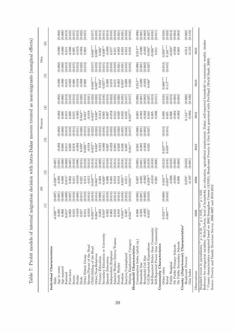
Tab

le7:

Pro

bit

model

sof

inte

rnal

mig

rati

ondec

isio

nw

ith

intr

a-D

akar

mov

ers

trea

ted

asnon

-mig

rants

(mar

ginal

effec

ts)

All

Wom

enM

en(1

)(2

)(3

)(4

)(5

)(6

)

Individ

ualCharacte

ristics

Male

-0.0

20∗∗∗

(0.0

07)

-0.0

20∗∗∗

(0.0

07)

Age

inyea

rs-0

.001

(0.0

01)

-0.0

01

(0.0

01)

-0.0

02

(0.0

02)

-0.0

02

(0.0

02)

-0.0

00

(0.0

02)

-0.0

00

(0.0

02)

Age

squ

are

d0.0

00

(0.0

00)

0.0

00

(0.0

00)

0.0

00

(0.0

00)

0.0

00

(0.0

00)

-0.0

00

(0.0

00)

-0.0

00

(0.0

00)

Fost

ered

0.0

15∗

(0.0

09)

0.0

15∗

(0.0

09)

0.0

14

(0.0

13)

0.0

13

(0.0

13)

0.0

15

(0.0

13)

0.0

14

(0.0

13)

Fir

st-b

orn

0.0

03

(0.0

07)

0.0

02

(0.0

07)

0.0

09

(0.0

10)

0.0

09

(0.0

10)

-0.0

05

(0.0

10)

-0.0

06

(0.0

10)

Ser

ere

0.0

13

(0.0

10)

0.0

11

(0.0

10)

0.0

18

(0.0

14)

0.0

15

(0.0

14)

0.0

08

(0.0

15)

0.0

05

(0.0

15)

Pou

lar

-0.0

10

(0.0

08)

-0.0

10

(0.0

08)

-0.0

03

(0.0

11)

-0.0

05

(0.0

12)

-0.0

16

(0.0

12)

-0.0

13

(0.0

12)

Dio

la0.0

17

(0.0

15)

0.0

21

(0.0

15)

0.0

39∗

(0.0

20)

0.0

44∗∗

(0.0

20)

-0.0

08

(0.0

22)

-0.0

04

(0.0

22)

Oth

erE

thn

icG

rou

p0.0

14

(0.0

10)

0.0

14

(0.0

10)

0.0

26∗∗

(0.0

13)

0.0

24∗

(0.0

14)

0.0

00

(0.0

14)

0.0

03

(0.0

15)

Sp

ou

se/P

are

nt

of

the

Hea

d-0

.010

(0.0

14)

-0.0

11

(0.0

14)

-0.0

18

(0.0

21)

-0.0

19

(0.0

21)

Ch

ild

/S

iblin

gof

the

Hea

d0.0

50∗∗∗

(0.0

13)

0.0

49∗∗∗

(0.0

13)

0.0

52∗∗

(0.0

23)

0.0

52∗∗

(0.0

23)

0.0

46∗∗∗

(0.0

17)

0.0

46∗∗∗

(0.0

17)

Oth

er/N

on

-Rel

ati

ves

0.0

64∗∗∗

(0.0

14)

0.0

64∗∗∗

(0.0

14)

0.0

40∗

(0.0

23)

0.0

40∗

(0.0

23)

0.0

97∗∗∗

(0.0

19)

0.0

99∗∗∗

(0.0

19)

Pri

mary

Ed

uca

tion

0.0

03

(0.0

09)

0.0

04

(0.0

09)

-0.0

15

(0.0

12)

-0.0

13

(0.0

13)

0.0

24∗

(0.0

14)

0.0

26∗

(0.0

14)

Sec

on

dary

Ed

uca

tion

or

Un

iver

sity

0.0

18∗

(0.0

11)

0.0

20∗

(0.0

11)

-0.0

00

(0.0

16)

0.0

05

(0.0

16)

0.0

37∗∗

(0.0

15)

0.0

38∗∗

(0.0

15)

Qu

ran

icE

du

cati

on

0.0

02

(0.0

10)

0.0

00

(0.0

10)

0.0

07

(0.0

13)

0.0

07

(0.0

13)

0.0

00

(0.0

14)

-0.0

03

(0.0

14)

Ind

epen

den

t/E

mp

loyer

0.0

02

(0.0

14)

0.0

05

(0.0

14)

-0.0

23

(0.0

23)

-0.0

18

(0.0

23)

0.0

19

(0.0

18)

0.0

17

(0.0

18)

Sala

ried

Work

er/In

tern

/T

rain

ee0.0

10

(0.0

14)

0.0

12

(0.0

14)

0.0

04

(0.0

23)

0.0

12

(0.0

23)

0.0

11

(0.0

18)

0.0

11

(0.0

18)

Fam

ily

Work

er0.0

19

(0.0

14)

0.0

18

(0.0

14)

0.0

29

(0.0

20)

0.0

29

(0.0

20)

0.0

03

(0.0

21)

0.0

03

(0.0

21)

Stu

den

t0.0

34∗∗

(0.0

16)

0.0

35∗∗

(0.0

16)

0.0

28

(0.0

25)

0.0

32

(0.0

25)

0.0

35∗

(0.0

21)

0.0

34

(0.0

21)

Inact

ive/

Un

emp

loyed

0.0

07

(0.0

12)

0.0

11

(0.0

12)

0.0

07

(0.0

16)

0.0

16

(0.0

17)

0.0

09

(0.0

18)

0.0

13

(0.0

19)

Mis

sin

gE

mp

loym

ent

Cate

gory

0.0

34∗∗∗

(0.0

12)

0.0

34∗∗∗

(0.0

12)

0.0

41∗∗

(0.0

17)

0.0

47∗∗∗

(0.0

17)

0.0

20

(0.0

16)

0.0

18

(0.0

16)

House

hold

Characte

ristics

Con

sum

pti

on

Ind

ex(a

du

lteq

.)0.0

06

(0.0

04)

0.0

07

(0.0

05)

0.0

01

(0.0

06)

0.0

03

(0.0

06)

0.0

14∗∗

(0.0

06)

0.0

14∗∗

(0.0

06)

Hou

seh

old

Siz

e-0

.001

(0.0

01)

-0.0

01

(0.0

01)

-0.0

01

(0.0

01)

-0.0

01

(0.0

01)

-0.0

00

(0.0

01)

-0.0

00

(0.0

01)

Hou

seh

old

Cel

lS

ize

-0.0

02

(0.0

02)

-0.0

02

(0.0

02)

-0.0

02

(0.0

03)

-0.0

02

(0.0

03)

-0.0

02

(0.0

03)

-0.0

03

(0.0

03)

Cel

l/H

ou

seh

old

Exp

end

itu

re0.0

35∗

(0.0

19)

0.0

38∗∗

(0.0

19)

0.0

25

(0.0

27)

0.0

24

(0.0

27)

0.0

46∗

(0.0

27)

0.0

50∗

(0.0

27)

Sel

f-R

eport

edR

ich

erth

an

Com

mu

nit

y-0

.010

(0.0

10)

0.0

05

(0.0

13)

-0.0

36∗∗

(0.0

16)

Sel

f-R

eport

edP

oore

rth

an

Com

mu

nit

y0.0

01

(0.0

08)

-0.0

06

(0.0

11)

0.0

11

(0.0

11)

Com

munity

Characte

ristics

Oth

erci

ties

0.0

52∗∗∗

(0.0

09)

0.0

31∗∗

(0.0

12)

0.0

37∗∗∗

(0.0

13)

0.0

09

(0.0

16)

0.0

68∗∗∗

(0.0

14)

0.0

59∗∗∗

(0.0

18)

Ru

ral

0.0

83∗∗∗

(0.0

10)

0.0

53∗∗∗

(0.0

16)

0.0

59∗∗∗

(0.0

14)

0.0

21

(0.0

21)

0.1

17∗∗∗

(0.0

15)

0.1

01∗∗∗

(0.0

23)

Pu

blic

Hosp

ital

-0.0

08

(0.0

10)

0.0

06

(0.0

13)

-0.0

24∗

(0.0

14)

Nb

Pu

blic

Pri

mary

Sch

ools

-0.0

03

(0.0

03)

-0.0

04

(0.0

04)

-0.0

04

(0.0

04)

Nb

Pu

blic

Sec

on

dary

Sch

ools

0.0

00

(0.0

03)

-0.0

02

(0.0

04)

0.0

03

(0.0

04)

County

(Depart

em

en

t)Characte

ristics†

Hea

dco

unt

Pover

ty0.0

78∗

(0.0

43)

0.1

44∗∗

(0.0

60)

-0.0

11

(0.0

62)

Gin

iIn

dex

-0.1

07

(0.0

81)

-0.0

93

(0.1

09)

-0.1

55

(0.1

19)

Ob

serv

ati

on

s6906

6906

3842

3842

3043

3043

Sta

nd

ard

erro

rsin

pare

nth

eses

,∗p<

0.1

0,∗∗p<

0.0

5,∗∗∗p<

0.0

1R

efer

ence

for

cate

gori

cal

vari

ab

les:

Wolo

f/L

ebou

,h

ead

of

hou

seh

old

,n

oed

uca

tion

,agri

cult

ura

lem

plo

ym

ent,

Dakar,

self

-rep

ort

edh

ou

seh

old

vs

com

mu

nit

yw

ealt

h:

sim

ilar

†C

ou

nty

chara

cter

isti

csco

mp

ute

db

ase

don

2002

Sen

egale

seC

ensu

s(A

NS

D);

Hea

dco

unt

Pover

ty&

Gin

iIn

dex

gen

erate

dw

ith

PovM

ap

2(W

orl

dB

an

k,

2009)

Sou

rce:

Pover

tyan

dF

am

ily

Str

uct

ure

Su

rvey

,2006-2

007

an

d2010-2

012

39

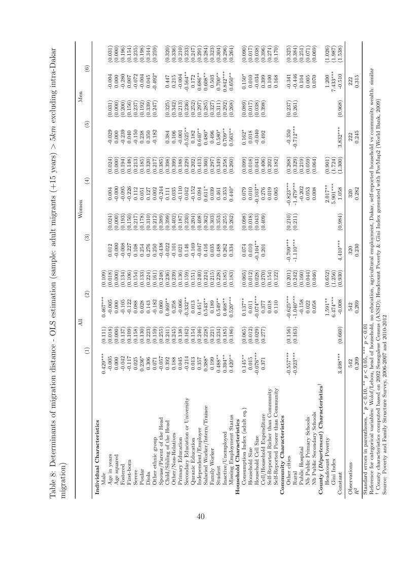
Tab

le8:

Det

erm

inan

tsof

mig

rati

ondis

tance

-O

LS

esti

mat

ion

(sam

ple

:ad

ult

mig

rants

(+15

year

s)>

5km

excl

udin

gin

tra-

Dak

arm

igra

tion

)

All

Wom

enM

en(1

)(2

)(3

)(4

)(5

)(6

)

Individ

ualCharacte

ristics

Male

0.4

29∗∗∗

(0.1

11)

0.4

67∗∗∗

(0.1

09)

Age

inyea

rs-0

.005

(0.0

18)

-0.0

05

(0.0

18)

0.0

12

(0.0

24)

0.0

04

(0.0

24)

-0.0

29

(0.0

31)

-0.0

04

(0.0

31)

Age

squ

are

d0.0

00

(0.0

00)

0.0

00

(0.0

00)

-0.0

00

(0.0

00)

-0.0

00

(0.0

00)

0.0

00

(0.0

00)

0.0

00

(0.0

00)

Fost

ered

-0.0

42

(0.1

37)

-0.1

05

(0.1

34)

-0.0

08

(0.1

93)

-0.0

95

(0.1

94)

-0.2

39

(0.2

00)

-0.2

80

(0.1

96)

Fir

st-b

orn

-0.1

17

(0.1

09)

-0.1

22

(0.1

06)

-0.2

27

(0.1

50)

-0.2

26

(0.1

48)

0.0

40

(0.1

56)

0.0

07

(0.1

54)

Ser

ere

0.0

25

(0.1

58)

0.0

88

(0.1

54)

0.1

08

(0.2

17)

0.1

12

(0.2

13)

-0.1

50

(0.2

37)

-0.0

72

(0.2

35)

Pou

lar

0.2

36∗

(0.1

30)

0.0

28

(0.1

33)

0.2

54

(0.1

78)

0.0

51

(0.1

85)

0.2

38

(0.1

92)

-0.0

04

(0.1

98)

Dio

la0.3

06

(0.2

23)

0.1

43

(0.2

24)

0.2

76

(0.3

10)

0.1

27

(0.3

20)

0.3

50

(0.3

39)

0.0

45

(0.3

44)

Oth

eret

hn

icgro

up

0.0

71

(0.1

59)

-0.1

82

(0.1

61)

0.2

50

(0.2

12)

0.0

02

(0.2

17)

-0.1

82

(0.2

47)

-0.4

92∗

(0.2

59)

Sp

ou

se/P

are

nt

of

the

Hea

d-0

.057

(0.2

55)

0.0

60

(0.2

48)

-0.4

38

(0.3

89)

-0.2

44

(0.3

85)

Ch

ild

/S

iblin

gof

the

Hea

d0.3

92

(0.2

41)

0.4

69∗∗

(0.2

36)

-0.0

22

(0.3

99)

0.1

11

(0.3

98)

0.3

84

(0.3

25)

0.4

47

(0.3

20)

Oth

er/N

on

-Rel

ati

ves

0.1

88

(0.2

45)

0.2

58

(0.2

39)

-0.1

01

(0.4

02)

0.0

35

(0.3

99)

0.1

06

(0.3

42)

0.2

15

(0.3

36)

Pri

mary

Ed

uca

tion

0.0

45

(0.1

38)

-0.0

66

(0.1

36)

0.0

21

(0.1

87)

-0.1

10

(0.1

88)

-0.0

01

(0.2

13)

-0.0

04

(0.2

10)

Sec

on

dary

Ed

uca

tion

or

Un

iver

sity

-0.2

14

(0.1

62)

-0.3

32∗∗

(0.1

59)

0.1

46

(0.2

30)

0.0

42

(0.2

29)

-0.5

25∗∗

(0.2

36)

-0.5

64∗∗

(0.2

33)

Qu

ran

icE

du

cati

on

0.0

13

(0.1

54)

0.0

13

(0.1

51)

-0.1

69

(0.2

04)

-0.1

52

(0.2

02)

0.1

82

(0.2

52)

0.1

72

(0.2

47)

Ind

epen

den

t/E

mp

loyer

0.3

57

(0.2

46)

0.4

51∗

(0.2

40)

-0.0

47

(0.4

08)

0.0

94

(0.4

13)

0.6

40∗∗

(0.2

97)

0.6

86∗∗

(0.2

91)

Sala

ried

Work

er/In

tern

/T

rain

ee0.3

88∗

(0.2

28)

0.5

43∗∗

(0.2

24)

0.4

16

(0.3

62)

0.6

11∗

(0.3

60)

0.4

80∗

(0.2

85)

0.6

08∗∗

(0.2

84)

Fam

ily

Work

er0.1

99

(0.2

21)

0.1

89

(0.2

15)

0.0

35

(0.3

03)

0.0

39

(0.2

97)

0.4

96

(0.3

27)

0.5

03

(0.3

23)

Stu

den

t0.4

88∗∗

(0.2

34)

0.5

49∗∗

(0.2

28)

0.4

88

(0.3

53)

0.4

61

(0.3

49)

0.5

80∗

(0.3

11)

0.7

00∗∗

(0.3

04)

Inact

ive/

Un

emp

loyed

0.3

94∗∗

(0.1

85)

0.4

68∗∗

(0.1

85)

0.2

62

(0.2

55)

0.3

53

(0.2

58)

0.7

09∗∗

(0.2

92)

0.8

42∗∗∗

(0.2

96)

Mis

sin

gE

mp

loym

ent

Sta

tus

0.4

20∗∗

(0.1

86)

0.5

20∗∗∗

(0.1

83)

0.3

34

(0.2

62)

0.4

40∗

(0.2

60)

0.5

63∗∗

(0.2

68)

0.6

50∗∗

(0.2

64)

House

hold

Characte

ristics

Con

sum

pti

on

Ind

ex(a

du

lteq

.)0.1

45∗∗

(0.0

65)

0.1

37∗∗

(0.0

65)

0.0

74

(0.0

98)

0.0

79

(0.0

99)

0.1

62∗

(0.0

89)

0.1

50∗

(0.0

90)

Hou

seh

old

Siz

e0.0

15

(0.0

12)

0.0

11

(0.0

12)

0.0

10

(0.0

18)

0.0

10

(0.0

18)

0.0

18

(0.0

17)

0.0

10

(0.0

17)

Hou

seh

old

Cel

lS

ize

-0.0

76∗∗∗

(0.0

29)

-0.0

74∗∗∗

(0.0

28)

-0.1

04∗∗

(0.0

43)

-0.1

03∗∗

(0.0

43)

-0.0

40

(0.0

38)

-0.0

34

(0.0

38)

Cel

l/H

ou

seh

old

Exp

end

itu

re0.3

71

(0.2

77)

0.3

77

(0.2

70)

0.2

01

(0.4

09)

0.2

76

(0.4

06)

0.4

92

(0.3

98)

0.3

99

(0.3

96)

Sel

f-R

eport

edR

ich

erth

an

Com

mu

nit

y0.0

18

(0.1

54)

0.0

19

(0.2

02)

0.1

00

(0.2

74)

Sel

f-R

eport

edP

oore

rth

an

Com

mu

nit

y0.1

10

(0.1

22)

0.0

65

(0.1

82)

0.1

68

(0.1

70)

Com

munity

Characte

ristics

Oth

erci

ties

-0.5

57∗∗∗

(0.1

56)

-0.6

25∗∗∗

(0.2

01)

-0.7

09∗∗∗

(0.2

10)

-0.8

23∗∗∗

(0.2

68)

-0.3

50

(0.2

37)

-0.3

41

(0.3

25)

Ru

ral

-0.9

23∗∗∗

(0.1

63)

-1.0

40∗∗∗

(0.2

42)

-1.1

10∗∗∗

(0.2

11)

-1.4

79∗∗∗

(0.3

29)

-0.7

12∗∗∗

(0.2

61)

-0.4

46

(0.3

84)

Pu

blic

Hosp

ital

-0.1

58

(0.1

60)

-0.2

02

(0.2

19)

0.1

04

(0.2

51)

Nb

Pu

blic

Pri

mary

Sch

ools

0.0

22

(0.0

44)

0.0

53

(0.0

59)

0.0

05

(0.0

71)

Nb

Pu

blic

Sec

on

dary

Sch

ools

0.0

58

(0.0

46)

0.0

08

(0.0

64)

0.0

70

(0.0

69)

County

(Depart

em

en

t)Characte

ristics†

Hea

dco

unt

Pover

ty1.5

91∗∗

(0.6

52)

2.0

17∗∗

(0.9

01)

1.2

00

(1.0

26)

Gin

iIn

dex

6.4

74∗∗∗

(1.2

56)

5.9

01∗∗∗

(1.7

24)

7.4

33∗∗∗

(1.9

87)

Con

stant

3.4

98∗∗∗

(0.6

60)

-0.0

08

(0.9

30)

4.4

10∗∗∗

(0.9

84)

1.0

58

(1.3

00)

3.8

32∗∗∗

(0.9

68)

-0.5

10

(1.5

38)

Ob

serv

ati

on

s542

542

320

320

222

222

R2

0.2

09

0.2

69

0.2

30

0.2

82

0.2

45

0.3

15

Sta

nd

ard

erro

rsin

pare

nth

eses

,∗p<

0.1

0,∗∗p<

0.0

5,∗∗∗p<

0.0

1R

efer

ence

for

cate

gori

cal

vari

ab

les:

Wolo

f/L

ebou

,h

ead

of

hou

seh

old

,n

oed

uca

tion

,agri

cult

ura

lem

plo

ym

ent,

Dakar,

self

-rep

ort

edh

ou

seh

old

vs

com

mu

nit

yw

ealt

h:

sim

ilar

†C

ou

nty

chara

cter

isti

csco

mp

ute

db

ase

don

2002

Sen

egale

seC

ensu

s(A

NS

D);

Hea

dco

unt

Pover

ty&

Gin

iIn

dex

gen

erate

dw

ith

PovM

ap

2(W

orl

dB

an

k,

2009)

Sou

rce:

Pover

tyan

dF

am

ily

Str

uct

ure

Su

rvey

,2006-2

007

an

d2010-2

012

40

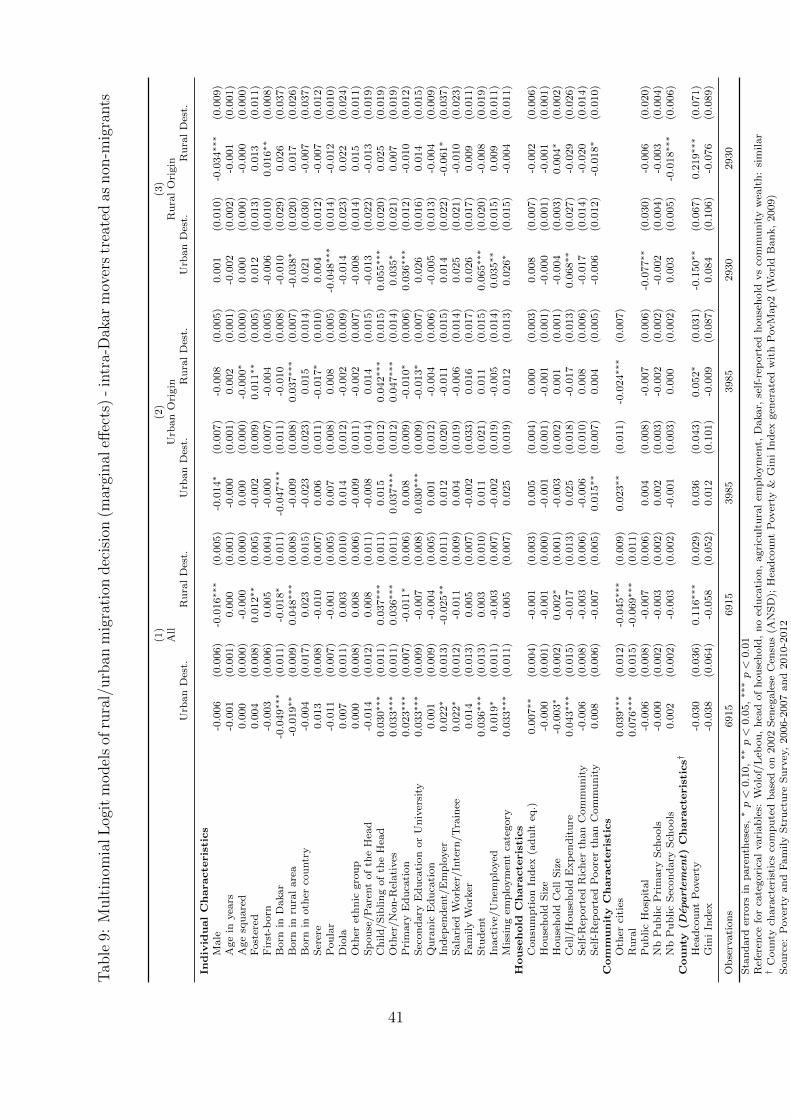
Tab

le9:

Mult

inom

ialL

ogit

model

sof

rura

l/urb

anm

igra

tion

dec

isio

n(m

argi

nal

effec

ts)

-in

tra-

Dak

arm

over

str

eate

das

non

-mig

rants

(1)

(2)

(3)

All

Urb

an

Ori

gin

Ru

ral

Ori

gin

Urb

an

Des

t.R

ura

lD

est.

Urb

an

Des

t.R

ura

lD

est.

Urb

an

Des

t.R

ura

lD

est.

Individ

ualCharacte

ristics

Male

-0.0

06

(0.0

06)

-0.0

16∗∗∗

(0.0

05)

-0.0

14∗

(0.0

07)

-0.0

08

(0.0

05)

0.0

01

(0.0

10)

-0.0

34∗∗∗

(0.0

09)

Age

inyea

rs-0

.001

(0.0

01)

0.0

00

(0.0

01)

-0.0

00

(0.0

01)

0.0

02

(0.0

01)

-0.0

02

(0.0

02)

-0.0

01

(0.0

01)

Age

squ

are

d0.0

00

(0.0

00)

-0.0

00

(0.0

00)

0.0

00

(0.0

00)

-0.0

00∗

(0.0

00)

0.0

00

(0.0

00)

-0.0

00

(0.0

00)

Fost

ered

0.0

04

(0.0

08)

0.0

12∗∗

(0.0

05)

-0.0

02

(0.0

09)

0.0

11∗∗

(0.0

05)

0.0

12

(0.0

13)

0.0

13

(0.0

11)

Fir

st-b

orn

-0.0

03

(0.0

06)

0.0

05

(0.0

04)

-0.0

00

(0.0

07)

-0.0

04

(0.0

05)

-0.0

06

(0.0

10)

0.0

16∗∗

(0.0

08)

Born

inD

akar

-0.0

49∗∗∗

(0.0

11)

-0.0

18∗

(0.0

11)

-0.0

47∗∗∗

(0.0

11)

-0.0

10

(0.0

08)

-0.0

10

(0.0

29)

0.0

26

(0.0

37)

Born

inru

ral

are

a-0

.019∗∗

(0.0

09)

0.0

48∗∗∗

(0.0

08)

-0.0

09

(0.0

08)

0.0

37∗∗∗

(0.0

07)

-0.0

38∗

(0.0

20)

0.0

17

(0.0

26)

Born

inoth

erco

untr

y-0

.004

(0.0

17)

0.0

23

(0.0

15)

-0.0

23

(0.0

23)

0.0

15

(0.0

14)

0.0

21

(0.0

30)

-0.0

07

(0.0

37)

Ser

ere

0.0

13

(0.0

08)

-0.0

10

(0.0

07)

0.0

06

(0.0

11)

-0.0

17∗

(0.0

10)

0.0

04

(0.0

12)

-0.0

07

(0.0

12)

Pou

lar

-0.0

11

(0.0

07)

-0.0

01

(0.0

05)

0.0

07

(0.0

08)

0.0

08

(0.0

05)

-0.0

48∗∗∗

(0.0

14)

-0.0

12

(0.0

10)

Dio

la0.0

07

(0.0

11)

0.0

03

(0.0

10)

0.0

14

(0.0

12)

-0.0

02

(0.0

09)

-0.0

14

(0.0

23)

0.0

22

(0.0

24)

Oth

eret

hn

icgro

up

0.0

00

(0.0

08)

0.0

08

(0.0

06)

-0.0

09

(0.0

11)

-0.0

02

(0.0

07)

-0.0

08

(0.0

14)

0.0

15

(0.0

11)

Sp

ou

se/P

are

nt

of

the

Hea

d-0

.014

(0.0

12)

0.0

08

(0.0

11)

-0.0

08

(0.0

14)

0.0

14

(0.0

15)

-0.0

13

(0.0

22)

-0.0

13

(0.0

19)

Ch

ild

/S

iblin

gof

the

Hea

d0.0

30∗∗∗

(0.0

11)

0.0

37∗∗∗

(0.0

11)

0.0

15

(0.0

12)

0.0

42∗∗∗

(0.0

15)

0.0

55∗∗∗

(0.0

20)

0.0

25

(0.0

19)

Oth

er/N

on

-Rel

ati

ves

0.0

33∗∗∗

(0.0

11)

0.0

36∗∗∗

(0.0

11)

0.0

37∗∗∗

(0.0

12)

0.0

47∗∗∗

(0.0

14)

0.0

35∗

(0.0

21)

0.0

07

(0.0

19)

Pri

mary

Ed

uca

tion

0.0

23∗∗∗

(0.0

07)

-0.0

11∗

(0.0

06)

0.0

08

(0.0

09)

-0.0

10∗

(0.0

06)

0.0

36∗∗∗

(0.0

12)

-0.0

10

(0.0

12)

Sec

on

dary

Ed

uca

tion

or

Un

iver

sity

0.0

33∗∗∗

(0.0

09)

-0.0

07

(0.0

08)

0.0

30∗∗∗

(0.0

09)

-0.0

13∗

(0.0

07)

0.0

26

(0.0

16)

0.0

14

(0.0

15)

Qu

ran

icE

du

cati

on

0.0

01

(0.0

09)

-0.0

04

(0.0

05)

0.0

01

(0.0

12)

-0.0

04

(0.0

06)

-0.0

05

(0.0

13)

-0.0

04

(0.0

09)

Ind

epen

den

t/E

mp

loyer

0.0

22∗

(0.0

13)

-0.0

25∗∗

(0.0

11)

0.0

12

(0.0

20)

-0.0

11

(0.0

15)

0.0

14

(0.0

22)

-0.0

61∗

(0.0

37)

Sala

ried

Work

er/In

tern

/T

rain

ee0.0

22∗

(0.0

12)

-0.0

11

(0.0

09)

0.0

04

(0.0

19)

-0.0

06

(0.0

14)

0.0

25

(0.0

21)

-0.0

10

(0.0

23)

Fam

ily

Work

er0.0

14

(0.0

13)

0.0

05

(0.0

07)

-0.0

02

(0.0

33)

0.0

16

(0.0

17)

0.0

26

(0.0

17)

0.0

09

(0.0

11)

Stu

den

t0.0

36∗∗∗

(0.0

13)

0.0

03

(0.0

10)

0.0

11

(0.0

21)

0.0

11

(0.0

15)

0.0

65∗∗∗

(0.0

20)

-0.0

08

(0.0

19)

Inact

ive/

Un

emp

loyed

0.0

19∗

(0.0

11)

-0.0

03

(0.0

07)

-0.0

02

(0.0

19)

-0.0

05

(0.0

14)

0.0

35∗∗

(0.0

15)

0.0

09

(0.0

11)

Mis

sin

gem

plo

ym

ent

cate

gory

0.0

33∗∗∗

(0.0

11)

0.0

05

(0.0

07)

0.0

25

(0.0

19)

0.0

12

(0.0

13)

0.0

26∗

(0.0

15)

-0.0

04

(0.0

11)

House

hold

Characte

ristics

Con

sum

pti

on

Ind

ex(a

du

lteq

.)0.0

07∗∗

(0.0

04)

-0.0

01

(0.0

03)

0.0

05

(0.0

04)

0.0

00

(0.0

03)

0.0

08

(0.0

07)

-0.0

02

(0.0

06)

Hou

seh

old

Siz

e-0

.000

(0.0

01)

-0.0

01

(0.0

00)

-0.0

01

(0.0

01)

-0.0

01

(0.0

01)

-0.0

00

(0.0

01)

-0.0

01

(0.0

01)

Hou

seh

old

Cel

lS

ize

-0.0

03∗

(0.0

02)

0.0

02∗

(0.0

01)

-0.0

03

(0.0

02)

0.0

01

(0.0

01)

-0.0

04

(0.0

03)

0.0

04∗

(0.0

02)

Cel

l/H

ou

seh

old

Exp

end

itu

re0.0

43∗∗∗

(0.0

15)

-0.0

17

(0.0

13)

0.0

25

(0.0

18)

-0.0

17

(0.0

13)

0.0

68∗∗

(0.0

27)

-0.0

29

(0.0

26)

Sel

f-R

eport

edR

ich

erth

an

Com

mu

nit

y-0

.006

(0.0

08)

-0.0

03

(0.0

06)

-0.0

06

(0.0

10)

0.0

08

(0.0

06)

-0.0

17

(0.0

14)

-0.0

20

(0.0

14)

Sel

f-R

eport

edP

oore

rth

an

Com

mu

nit

y0.0

08

(0.0

06)

-0.0

07

(0.0

05)

0.0

15∗∗

(0.0

07)

0.0

04

(0.0

05)

-0.0

06

(0.0

12)

-0.0

18∗

(0.0

10)

Com

munity

Characte

ristics

Oth

erci

ties

0.0

39∗∗∗

(0.0

12)

-0.0

45∗∗∗

(0.0

09)

0.0

23∗∗

(0.0

11)

-0.0

24∗∗∗

(0.0

07)

Ru

ral

0.0

76∗∗∗

(0.0

15)

-0.0

69∗∗∗

(0.0

11)

Pu

blic

Hosp

ital

-0.0

06

(0.0

08)

-0.0

07

(0.0

06)

0.0

04

(0.0

08)

-0.0

07

(0.0

06)

-0.0

77∗∗

(0.0

30)

-0.0

06

(0.0

20)

Nb

Pu

blic

Pri

mary

Sch

ools

-0.0

00

(0.0

02)

-0.0

03

(0.0

02)

0.0

02

(0.0

03)

-0.0

02

(0.0

02)

-0.0

02

(0.0

04)

-0.0

03

(0.0

04)

Nb

Pu

blic

Sec

on

dary

Sch

ools

0.0

02

(0.0

02)

-0.0

03

(0.0

02)

-0.0

01

(0.0

03)

0.0

00

(0.0

02)

0.0

03

(0.0

05)

-0.0

18∗∗∗

(0.0

06)

County

(Depart

em

en

t)Characte

ristics†

Hea

dco

unt

Pover

ty-0

.030

(0.0

36)

0.1

16∗∗∗

(0.0

29)

0.0

36

(0.0

43)

0.0

52∗

(0.0

31)

-0.1

50∗∗

(0.0

67)

0.2

19∗∗∗

(0.0

71)

Gin

iIn

dex

-0.0

38

(0.0

64)

-0.0

58

(0.0

52)

0.0

12

(0.1

01)

-0.0

09

(0.0

87)

0.0

84

(0.1

06)

-0.0

76

(0.0

89)

Ob

serv

ati

on

s6915

6915

3985

3985

2930

2930

Sta

nd

ard

erro

rsin

pare

nth

eses

,∗p<

0.1

0,∗∗p<

0.0

5,∗∗∗p<

0.0

1R

efer

ence

for

cate

gori

cal

vari

ab

les:

Wolo

f/L

ebou

,h

ead

of

hou

seh

old

,n

oed

uca

tion

,agri

cult

ura

lem

plo

ym

ent,

Dakar,

self

-rep

ort

edh

ou

seh

old

vs

com

mu

nit

yw

ealt

h:

sim

ilar

†C

ou

nty

chara

cter

isti

csco

mp

ute

db

ase

don

2002

Sen

egale

seC

ensu

s(A

NS

D);

Hea

dco

unt

Pover

ty&

Gin

iIn

dex

gen

erate

dw

ith

PovM

ap

2(W

orl

dB

an

k,

2009)

Sou

rce:

Pover

tyan

dF

am

ily

Str

uct

ure

Su

rvey

,2006-2

007

an

d2010-2

012

41

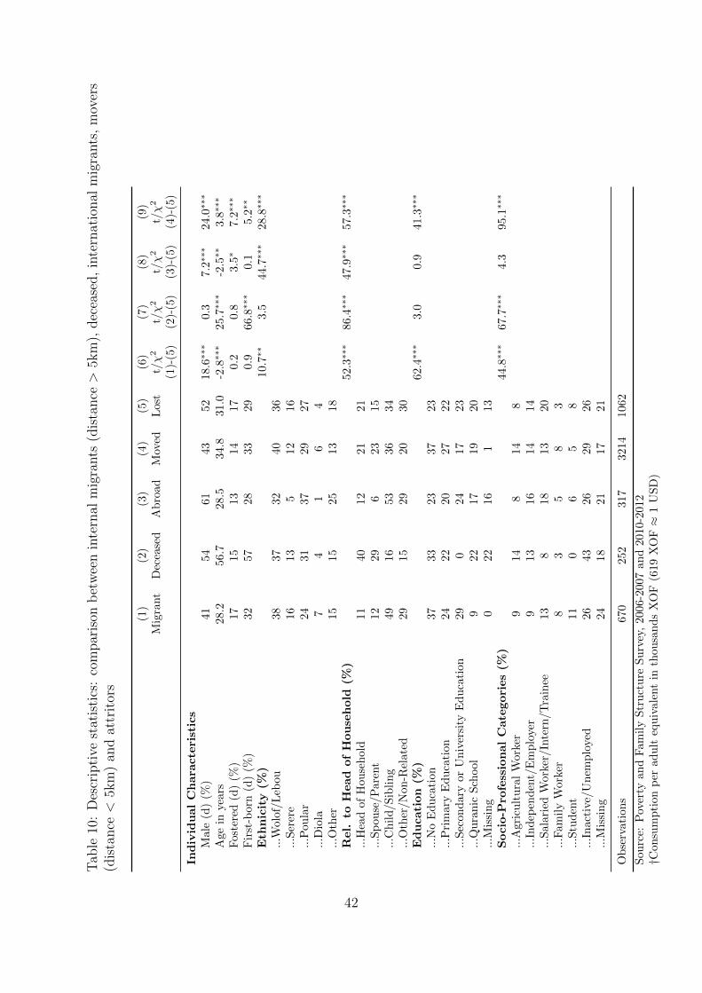
Tab

le10

:D

escr

ipti

vest

atis

tics

:co

mpar

ison

bet

wee

nin

tern

alm

igra

nts

(dis

tance>

5km

),dec

ease

d,

inte

rnat

ional

mig

rants

,m

over

s(d

ista

nce<

5km

)an

dat

trit

ors

(1)

(2)

(3)

(4)

(5)

(6)

(7)

(8)

(9)

Mig

rant

Dec

ease

dA

bro

ad

Mov

edL

ost

t/χ2

t/χ2

t/χ2

t/χ2

(1)-

(5)

(2)-

(5)

(3)-

(5)

(4)-

(5)

IndividualChara

cteristics

Mal

e(d

)(%

)41

54

61

43

52

18.6∗∗∗

0.3

7.2∗∗∗

24.0∗∗∗

Age

inye

ars

28.2

56.7

28.5

34.8

31.0

-2.8∗∗∗

25.7∗∗∗

-2.5∗∗

3.8∗∗∗

Fos

tere

d(d

)(%

)17

15

13

14

17

0.2

0.8

3.5∗

7.2∗∗∗

Fir

st-b

orn

(d)

(%)

3257

28

33

29

0.9

66.8∗∗∗

0.1

5.2∗∗

Eth

nicity(%

)10.7∗∗

3.5

44.7∗∗∗

28.8∗∗∗

...W

olof

/Leb

ou38

37

32

40

36

...S

erer

e16

13

512

16

...P

oula

r24

31

37

29

27

...D

iola

74

16

4..

.Oth

er15

15

25

13

18

Rel.

toHead

ofHousehold

(%)

52.3∗∗∗

86.4∗∗∗

47.9∗∗∗

57.3∗∗∗

...H

ead

ofH

ouse

hol

d11

40

12

21

21

...S

pou

se/P

aren

t12

29

623

15

...C

hil

d/S

ibli

ng

4916

53

36

34

...O

ther

/Non

-Rel

ated

2915

29

20

30

Education

(%)

62.4∗∗∗

3.0

0.9

41.3∗∗∗

...N

oE

du

cati

on37

33

23

37

23

...P

rim

ary

Ed

uca

tion

2422

20

27

22

...S

econ

dar

yor

Un

iver

sity

Ed

uca

tion

290

24

17

23

...Q

ura

nic

Sch

ool

922

17

19

20

...M

issi

ng

022

16

113

Socio-P

rofessionalCategories(%

)44.8∗∗∗

67.7∗∗∗

4.3

95.1∗∗∗

...A

gric

ult

ura

lW

orke

r9

14

814

8..

.In

dep

end

ent/

Em

plo

yer

913

16

14

14

...S

alar

ied

Wor

ker/

Inte

rn/T

rain

ee13

818

13

20

...F

amil

yW

orke

r8

35

83

...S

tud

ent

110

65

8..

.In

acti

ve/U

nem

plo

yed

2643

26

29

26

...M

issi

ng

2418

21

17

21

Ob

serv

atio

ns

670

252

317

3214

1062

Sou

rce:

Pov

erty

and

Fam

ily

Str

uct

ure

Su

rvey

,20

06-2

007

and

2010-2

012

†Con

sum

pti

onp

erad

ult

equ

ival

ent

inth

ousa

nd

sX

OF

(619

XO

F≈

1U

SD

)

42

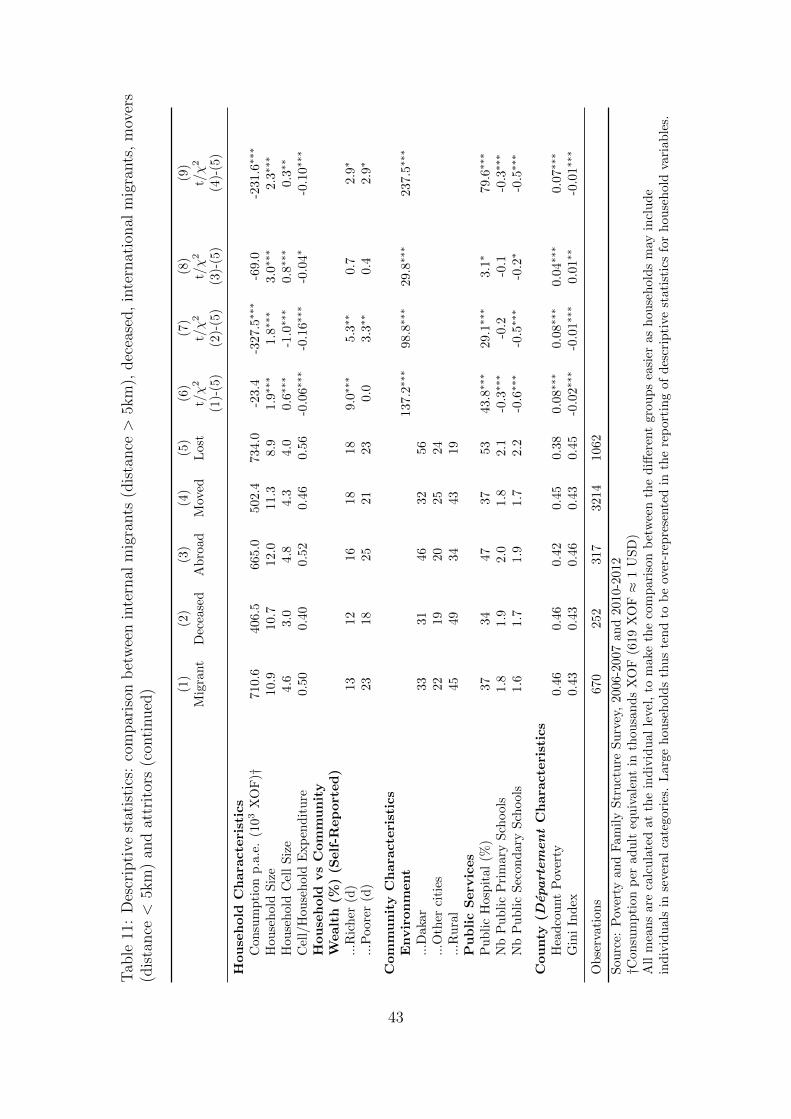
Tab

le11

:D

escr

ipti

vest

atis

tics

:co

mpar

ison

bet

wee

nin

tern

alm

igra

nts

(dis

tance>

5km

),dec

ease

d,

inte

rnat

ional

mig

rants

,m

over

s(d

ista

nce<

5km

)an

dat

trit

ors

(con

tinued

) (1)

(2)

(3)

(4)

(5)

(6)

(7)

(8)

(9)

Mig

rant

Dec

ease

dA

bro

ad

Mov

edL

ost

t/χ2

t/χ2

t/χ2

t/χ2

(1)-

(5)

(2)-

(5)

(3)-

(5)

(4)-

(5)

Household

Chara

cteristics

Con

sum

pti

onp

.a.e

.(1

03X

OF

)†71

0.6

406.5

665.0

502.4

734.0

-23.4

-327.5∗∗∗

-69.0

-231.6∗∗∗

Hou

seh

old

Siz

e10

.910.7

12.0

11.3

8.9

1.9∗∗∗

1.8∗∗∗

3.0∗∗∗

2.3∗∗∗

Hou

seh

old

Cel

lS

ize

4.6

3.0

4.8

4.3

4.0

0.6∗∗∗

-1.0∗∗∗

0.8∗∗∗

0.3∗∗

Cel

l/H

ouse

hol

dE

xp

end

itu

re0.

50

0.4

00.5

20.4

60.5

6-0

.06∗∗∗

-0.1

6∗∗∗

-0.0

4∗

-0.1

0∗∗∗

Household

vsCommunity

Wealth

(%)(S

elf-R

eported)

...R

ich

er(d

)13

12

16

18

18

9.0∗∗∗

5.3∗∗

0.7

2.9∗

...P

oor

er(d

)23

18

25

21

23

0.0

3.3∗∗

0.4

2.9∗

CommunityChara

cteristics

Environment

137.2∗∗∗

98.8∗∗∗

29.8∗∗∗

237.5∗∗∗

...D

akar

3331

46

32

56

...O

ther

citi

es22

19

20

25

24

...R

ura

l45

49

34

43

19

PublicServ

ices

Pu

bli

cH

osp

ital

(%)

3734

47

37

53

43.8∗∗∗

29.1∗∗∗

3.1∗

79.6∗∗∗

Nb

Pu

bli

cP

rim

ary

Sch

ool

s1.

81.9

2.0

1.8

2.1

-0.3∗∗∗

-0.2

-0.1

-0.3∗∗∗

Nb

Pu

bli

cS

econ

dar

yS

chool

s1.

61.7

1.9

1.7

2.2

-0.6∗∗∗

-0.5∗∗∗

-0.2∗

-0.5∗∗∗

County

(Depart

em

en

tChara

cteristics

Hea

dco

unt

Pov

erty

0.46

0.4

60.4

20.4

50.3

80.0

8∗∗∗

0.0

8∗∗∗

0.0

4∗∗∗

0.0

7∗∗∗

Gin

iIn

dex

0.43

0.4

30.4

60.4

30.4

5-0

.02∗∗∗

-0.0

1∗∗∗

0.0

1∗∗

-0.0

1∗∗∗

Ob

serv

atio

ns

670

252

317

3214

1062

Sou

rce:

Pov

erty

and

Fam

ily

Str

uct

ure

Su

rvey

,20

06-2

007

and

2010-2

012

†Con

sum

pti

onp

erad

ult

equ

ival

ent

inth

ousa

nd

sX

OF

(619

XO

F≈

1U

SD

)A

llm

ean

sar

eca

lcu

late

dat

the

ind

ivid

ual

leve

l,to

make

the

com

pari

son

bet

wee

nth

ed

iffer

ent

gro

up

sea

sier

as

hou

seh

old

sm

ayin

clu

de

ind

ivid

ual

sin

seve

ral

cate

gori

es.

Lar

geh

ouse

hol

ds

thu

ste

nd

tob

eov

er-r

epre

sente

din

the

rep

ort

ing

of

des

crip

tive

stati

stic

sfo

rh

ou

seh

old

vari

ab

les.

43

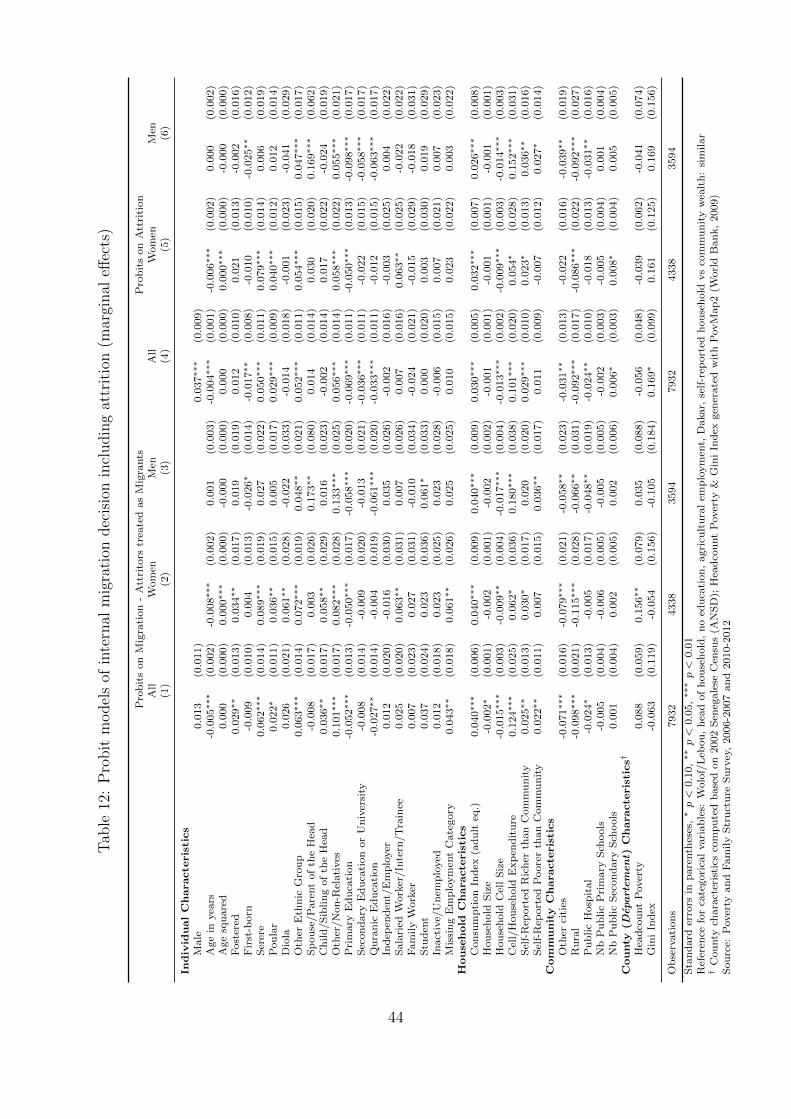
Tab

le12

:P

robit

model

sof

inte

rnal

mig

rati

ondec

isio

nin

cludin

gat

trit

ion

(mar

ginal

effec

ts)

Pro

bit

son

Mig

rati

on

-A

ttri

tors

trea

ted

as

Mig

rants

Pro

bit

son

Att

riti

on

All

Wom

enM

enA

llW

om

enM

en(1

)(2

)(3

)(4

)(5

)(6

)

Individ

ualCharacte

ristics

Male

0.0

13

(0.0

11)

0.0

37∗∗∗

(0.0

09)

Age

inyea

rs-0

.005∗∗∗

(0.0

02)

-0.0

08∗∗∗

(0.0

02)

0.0

01

(0.0

03)

-0.0

04∗∗∗

(0.0

01)

-0.0

06∗∗∗

(0.0

02)

0.0

00

(0.0

02)

Age

squ

are

d0.0

00

(0.0

00)

0.0

00∗∗∗

(0.0

00)

-0.0

00

(0.0

00)

0.0

00

(0.0

00)

0.0

00∗∗∗

(0.0

00)

-0.0

00

(0.0

00)

Fost

ered

0.0

29∗∗

(0.0

13)

0.0

34∗∗

(0.0

17)

0.0

19

(0.0

19)

0.0

12

(0.0

10)

0.0

21

(0.0

13)

-0.0

02

(0.0

16)

Fir

st-b

orn

-0.0

09

(0.0

10)

0.0

04

(0.0

13)

-0.0

26∗

(0.0

14)

-0.0

17∗∗

(0.0

08)

-0.0

10

(0.0

10)

-0.0

25∗∗

(0.0

12)

Ser

ere

0.0

62∗∗∗

(0.0

14)

0.0

89∗∗∗

(0.0

19)

0.0

27

(0.0

22)

0.0

50∗∗∗

(0.0

11)

0.0

79∗∗∗

(0.0

14)

0.0

06

(0.0

19)

Pou

lar

0.0

22∗

(0.0

11)

0.0

36∗∗

(0.0

15)

0.0

05

(0.0

17)

0.0

29∗∗∗

(0.0

09)

0.0

40∗∗∗

(0.0

12)

0.0

12

(0.0

14)

Dio

la0.0

26

(0.0

21)

0.0

61∗∗

(0.0

28)

-0.0

22

(0.0

33)

-0.0

14

(0.0

18)

-0.0

01

(0.0

23)

-0.0

41

(0.0

29)

Oth

erE

thn

icG

rou

p0.0

63∗∗∗

(0.0

14)

0.0

72∗∗∗

(0.0

19)

0.0

48∗∗

(0.0

21)

0.0

52∗∗∗

(0.0

11)

0.0

54∗∗∗

(0.0

15)

0.0

47∗∗∗

(0.0

17)

Sp

ou

se/P

are

nt

of

the

Hea

d-0

.008

(0.0

17)

0.0

03

(0.0

26)

0.1

73∗∗

(0.0

80)

0.0

14

(0.0

14)

0.0

30

(0.0

20)

0.1

69∗∗∗

(0.0

62)

Ch

ild

/S

iblin

gof

the

Hea

d0.0

36∗∗

(0.0

17)

0.0

58∗∗

(0.0

29)

0.0

16

(0.0

23)

-0.0

02

(0.0

14)

0.0

17

(0.0

22)

-0.0

24

(0.0

19)

Oth

er/N

on

-Rel

ati

ves

0.1

01∗∗∗

(0.0

17)

0.0

82∗∗∗

(0.0

28)

0.1

33∗∗∗

(0.0

25)

0.0

56∗∗∗

(0.0

14)

0.0

58∗∗∗

(0.0

22)

0.0

55∗∗∗

(0.0

21)

Pri

mary

Ed

uca

tion

-0.0

52∗∗∗

(0.0

13)

-0.0

50∗∗∗

(0.0

17)

-0.0

58∗∗∗

(0.0

20)

-0.0

69∗∗∗

(0.0

11)

-0.0

50∗∗∗

(0.0

13)

-0.0

98∗∗∗

(0.0

17)

Sec

on

dary

Ed

uca

tion

or

Un

iver

sity

-0.0

08

(0.0

14)

-0.0

09

(0.0

20)

-0.0

13

(0.0

21)

-0.0

36∗∗∗

(0.0

11)

-0.0

22

(0.0

15)

-0.0

58∗∗∗

(0.0

17)

Qu

ran

icE

du

cati

on

-0.0

27∗∗

(0.0

14)

-0.0

04

(0.0

19)

-0.0

61∗∗∗

(0.0

20)

-0.0

33∗∗∗

(0.0

11)

-0.0

12

(0.0

15)

-0.0

63∗∗∗

(0.0

17)

Ind

epen

den

t/E

mp

loyer

0.0

12

(0.0

20)

-0.0

16

(0.0

30)

0.0

35

(0.0

26)

-0.0

02

(0.0

16)

-0.0

03

(0.0

25)

0.0

04

(0.0

22)

Sala

ried

Work

er/In

tern

/T

rain

ee0.0

25

(0.0

20)

0.0

63∗∗

(0.0

31)

0.0

07

(0.0

26)

0.0

07

(0.0

16)

0.0

63∗∗

(0.0

25)

-0.0

22

(0.0

22)

Fam

ily

Work

er0.0

07

(0.0

23)

0.0

27

(0.0

31)

-0.0

10

(0.0

34)

-0.0

24

(0.0

21)

-0.0

15

(0.0

29)

-0.0

18

(0.0

31)

Stu

den

t0.0

37

(0.0

24)

0.0

23

(0.0

36)

0.0

61∗

(0.0

33)

0.0

00

(0.0

20)

0.0

03

(0.0

30)

0.0

19

(0.0

29)

Inact

ive/

Un

emp

loyed

0.0

12

(0.0

18)

0.0

23

(0.0

25)

0.0

23

(0.0

28)

-0.0

06

(0.0

15)

0.0

07

(0.0

21)

0.0

07

(0.0

23)

Mis

sin

gE

mp

loym

ent

Cate

gory

0.0

43∗∗

(0.0

18)

0.0

61∗∗

(0.0

26)

0.0

25

(0.0

25)

0.0

10

(0.0

15)

0.0

23

(0.0

22)

0.0

03

(0.0

22)

House

hold

Characte

ristics

Con

sum

pti

on

Ind

ex(a

du

lteq

.)0.0

40∗∗∗

(0.0

06)

0.0

40∗∗∗

(0.0

09)

0.0

40∗∗∗

(0.0

09)

0.0

30∗∗∗

(0.0

05)

0.0

32∗∗∗

(0.0

07)

0.0

26∗∗∗

(0.0

08)

Hou

seh

old

Siz

e-0

.002∗

(0.0

01)

-0.0

02

(0.0

01)

-0.0

02

(0.0

02)

-0.0

01

(0.0

01)

-0.0

01

(0.0

01)

-0.0

01

(0.0

01)

Hou

seh

old

Cel

lS

ize

-0.0

15∗∗∗

(0.0

03)

-0.0

09∗∗

(0.0

04)

-0.0

17∗∗∗

(0.0

04)

-0.0

13∗∗∗

(0.0

02)

-0.0

09∗∗∗

(0.0

03)

-0.0

14∗∗∗

(0.0

03)

Cel

l/H

ou

seh

old

Exp

end

itu

re0.1

24∗∗∗

(0.0

25)

0.0

62∗

(0.0

36)

0.1

80∗∗∗

(0.0

38)

0.1

01∗∗∗

(0.0

20)

0.0

54∗

(0.0

28)

0.1

52∗∗∗

(0.0

31)

Sel

f-R

eport

edR

ich

erth

an

Com

mu

nit

y0.0

25∗∗

(0.0

13)

0.0

30∗

(0.0

17)

0.0

20

(0.0

20)

0.0

29∗∗∗

(0.0

10)

0.0

23∗

(0.0

13)

0.0

36∗∗

(0.0

16)

Sel

f-R

eport

edP

oore

rth

an

Com

mu

nit

y0.0

22∗∗

(0.0

11)

0.0

07

(0.0

15)

0.0

36∗∗

(0.0

17)

0.0

11

(0.0

09)

-0.0

07

(0.0

12)

0.0

27∗

(0.0

14)

Com

munity

Characte

ristics

Oth

erci

ties

-0.0

71∗∗∗

(0.0

16)

-0.0

79∗∗∗

(0.0

21)

-0.0

58∗∗

(0.0

23)

-0.0

31∗∗

(0.0

13)

-0.0

22

(0.0

16)

-0.0

39∗∗

(0.0

19)

Ru

ral

-0.0

98∗∗∗

(0.0

21)

-0.1

15∗∗∗

(0.0

28)

-0.0

66∗∗

(0.0

31)

-0.0

92∗∗∗

(0.0

17)

-0.0

86∗∗∗

(0.0

22)

-0.0

92∗∗∗

(0.0

27)

Pu

blic

Hosp

ital

-0.0

24∗

(0.0

13)

-0.0

05

(0.0

17)

-0.0

48∗∗

(0.0

19)

-0.0

24∗∗

(0.0

10)

-0.0

18

(0.0

13)

-0.0

31∗∗

(0.0

16)

Nb

Pu

blic

Pri

mary

Sch

ools

-0.0

05

(0.0

04)

-0.0

06

(0.0

05)

-0.0

05

(0.0

05)

-0.0

02

(0.0

03)

-0.0

05

(0.0

04)

0.0

01

(0.0

04)

Nb

Pu

blic

Sec

on

dary

Sch

ools

0.0

01

(0.0

04)

0.0

02

(0.0

05)

0.0

02

(0.0

06)

0.0

06∗

(0.0

03)

0.0

08∗

(0.0

04)

0.0

05

(0.0

05)

County

(Depart

em

en

t)Characte

ristics†

Hea

dco

unt

Pover

ty0.0

88

(0.0

59)

0.1

56∗∗

(0.0

79)

0.0

35

(0.0

88)

-0.0

56

(0.0

48)

-0.0

39

(0.0

62)

-0.0

41

(0.0

74)

Gin

iIn

dex

-0.0

63

(0.1

19)

-0.0

54

(0.1

56)

-0.1

05

(0.1

84)

0.1

69∗

(0.0

99)

0.1

61

(0.1

25)

0.1

69

(0.1

56)

Ob

serv

ati

on

s7932

4338

3594

7932

4338

3594

Sta

nd

ard

erro

rsin

pare

nth

eses

,∗p<

0.1

0,∗∗p<

0.0

5,∗∗∗p<

0.0

1R

efer

ence

for

cate

gori

cal

vari

ab

les:

Wolo

f/L

ebou

,h

ead

of

hou

seh

old

,n

oed

uca

tion

,agri

cult

ura

lem

plo

ym

ent,

Dakar,

self

-rep

ort

edh

ou

seh

old

vs

com

mu

nit

yw

ealt

h:

sim

ilar

†C

ou

nty

chara

cter

isti

csco

mp

ute

db

ase

don

2002

Sen

egale

seC

ensu

s(A

NS

D);

Hea

dco

unt

Pover

ty&

Gin

iIn

dex

gen

erate

dw

ith

PovM

ap

2(W

orl

dB

an

k,

2009)

Sou

rce:

Pover

tyan

dF

am

ily

Str

uct

ure

Su

rvey

,2006-2

007

an

d2010-2

012

44

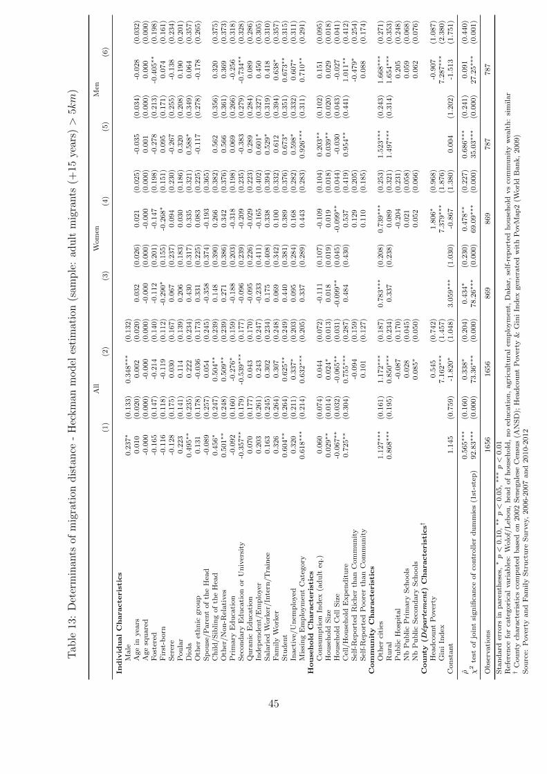
Tab

le13

:D

eter

min

ants

ofm

igra

tion

dis

tance

-H

eckm

anm

odel

esti

mat

ion

(sam

ple

:ad

ult

mig

rants

(+15

year

s)>

5km

)

All

Wom

enM

en(1

)(2

)(3

)(4

)(5

)(6

)

Individ

ualCharacte

ristics

Male

0.2

37∗

(0.1

33)

0.3

48∗∗∗

(0.1

32)

Age

inyea

rs0.0

10

(0.0

20)

0.0

02

(0.0

20)

0.0

32

(0.0

26)

0.0

21

(0.0

25)

-0.0

35

(0.0

34)

-0.0

28

(0.0

32)

Age

squ

are

d-0

.000

(0.0

00)

-0.0

00

(0.0

00)

-0.0

00

(0.0

00)

-0.0

00

(0.0

00)

0.0

01

(0.0

00)

0.0

00

(0.0

00)

Fost

ered

-0.1

65

(0.1

47)

-0.2

14

(0.1

40)

-0.1

12

(0.2

01)

-0.1

47

(0.1

98)

-0.2

78

(0.2

13)

-0.4

05∗∗

(0.1

98)

Fir

st-b

orn

-0.1

16

(0.1

18)

-0.1

19

(0.1

12)

-0.2

90∗

(0.1

55)

-0.2

68∗

(0.1

51)

0.0

95

(0.1

71)

0.0

74

(0.1

61)

Ser

ere

-0.1

28

(0.1

75)

0.0

30

(0.1

67)

0.0

67

(0.2

37)

0.0

94

(0.2

30)

-0.2

67

(0.2

55)

-0.1

38

(0.2

34)

Pou

lar

0.2

23

(0.1

41)

0.1

14

(0.1

39)

0.2

06

(0.1

83)

0.0

30

(0.1

86)

0.3

20

(0.2

08)

0.1

90

(0.2

01)

Dio

la0.4

95∗∗

(0.2

35)

0.2

22

(0.2

34)

0.4

30

(0.3

17)

0.3

35

(0.3

21)

0.5

88∗

(0.3

49)

0.0

64

(0.3

57)

Oth

eret

hn

icgro

up

0.1

31

(0.1

78)

-0.0

36

(0.1

73)

0.3

31

(0.2

25)

0.0

83

(0.2

25)

-0.1

17

(0.2

78)

-0.1

78

(0.2

65)

Sp

ou

se/P

are

nt

of

the

Hea

d-0

.089

(0.2

57)

0.0

54

(0.2

45)

-0.3

58

(0.3

74)

-0.1

93

(0.3

65)

Ch

ild

/S

iblin

gof

the

Hea

d0.4

56∗

(0.2

47)

0.5

04∗∗

(0.2

39)

0.1

48

(0.3

90)

0.2

66

(0.3

82)

0.5

62

(0.3

56)

0.3

20

(0.3

75)

Oth

er/N

on

-Rel

ati

ves

0.5

01∗∗

(0.2

48)

0.5

09∗∗

(0.2

39)

0.2

71

(0.3

86)

0.3

42

(0.3

76)

0.5

66

(0.3

61)

0.3

69

(0.3

73)

Pri

mary

Ed

uca

tion

-0.0

92

(0.1

60)

-0.2

76∗

(0.1

59)

-0.1

88

(0.2

03)

-0.3

18

(0.1

98)

0.0

69

(0.2

66)

-0.2

56

(0.3

18)

Sec

on

dary

Ed

uca

tion

or

Un

iver

sity

-0.3

57∗∗

(0.1

79)

-0.5

39∗∗∗

(0.1

77)

-0.0

96

(0.2

39)

-0.2

09

(0.2

35)

-0.3

83

(0.2

79)

-0.7

34∗∗

(0.3

28)

Qu

ran

icE

du

cati

on

0.0

70

(0.1

77)

0.0

43

(0.1

70)

-0.0

95

(0.2

26)

-0.0

29

(0.2

23)

0.2

89

(0.2

84)

0.0

89

(0.2

86)

Ind

epen

den

t/E

mp

loyer

0.2

03

(0.2

61)

0.2

43

(0.2

47)

-0.2

33

(0.4

11)

-0.1

65

(0.4

02)

0.6

01∗

(0.3

27)

0.4

50

(0.3

05)

Sala

ried

Work

er/In

tern

/T

rain

ee0.1

63

(0.2

45)

0.3

02

(0.2

34)

0.1

75

(0.4

08)

0.3

38

(0.3

94)

0.5

29∗

(0.3

19)

0.4

18

(0.3

10)

Fam

ily

Work

er0.3

26

(0.2

64)

0.3

07

(0.2

48)

0.0

69

(0.3

42)

0.1

00

(0.3

32)

0.6

12

(0.3

94)

0.6

38∗

(0.3

57)

Stu

den

t0.6

04∗∗

(0.2

64)

0.6

25∗∗

(0.2

49)

0.4

40

(0.3

81)

0.3

89

(0.3

76)

0.6

73∗

(0.3

51)

0.6

73∗∗

(0.3

15)

Inact

ive/

Un

emp

loyed

0.3

20

(0.2

11)

0.3

37∗

(0.2

03)

0.0

95

(0.2

84)

0.1

68

(0.2

82)

0.5

98∗

(0.3

32)

0.6

07∗

(0.3

11)

Mis

sin

gE

mp

loym

ent

Cate

gory

0.6

18∗∗∗

(0.2

14)

0.6

32∗∗∗

(0.2

05)

0.3

37

(0.2

89)

0.4

43

(0.2

83)

0.9

26∗∗∗

(0.3

11)

0.7

10∗∗

(0.2

91)

House

hold

Characte

ristics

Con

sum

pti

on

Ind

ex(a

du

lteq

.)0.0

60

(0.0

74)

0.0

44

(0.0

72)

-0.1

11

(0.1

07)

-0.1

09

(0.1

04)

0.2

03∗∗

(0.1

02)

0.1

51

(0.0

95)

Hou

seh

old

Siz

e0.0

29∗∗

(0.0

14)

0.0

24∗

(0.0

13)

0.0

18

(0.0

19)

0.0

19

(0.0

18)

0.0

39∗∗

(0.0

20)

0.0

29

(0.0

18)

Hou

seh

old

Cel

lS

ize

-0.0

67∗∗

(0.0

32)

-0.0

65∗∗

(0.0

31)

-0.0

99∗∗

(0.0

45)

-0.0

99∗∗

(0.0

44)

-0.0

30

(0.0

43)

-0.0

27

(0.0

41)

Cel

l/H

ou

seh

old

Exp

end

itu

re0.7

25∗∗

(0.3

04)

0.7

55∗∗∗

(0.2

87)

0.4

84

(0.4

30)

0.5

37

(0.4

19)

0.9

54∗∗

(0.4

41)

1.0

11∗∗

(0.4

12)

Sel

f-R

eport

edR

ich

erth

an

Com

mu

nit

y-0

.094

(0.1

59)

0.1

29

(0.2

05)

-0.4

79∗

(0.2

54)

Sel

f-R

eport

edP

oore

rth

an

Com

mu

nit

y0.1

01

(0.1

27)

0.1

10

(0.1

85)

0.0

88

(0.1

74)

Com

munity

Characte

ristics

Oth

erci

ties

1.1

27∗∗∗

(0.1

61)

1.1

72∗∗∗

(0.1

87)

0.7

83∗∗∗

(0.2

08)

0.7

39∗∗∗

(0.2

53)

1.5

23∗∗∗

(0.2

43)

1.6

68∗∗∗

(0.2

71)

Ru

ral

0.8

68∗∗∗

(0.1

95)

0.8

50∗∗∗

(0.2

34)

0.3

37

(0.2

38)

0.0

89

(0.3

21)

1.4

97∗∗∗

(0.3

14)

1.6

54∗∗∗

(0.3

53)

Pu

blic

Hosp

ital

-0.0

87

(0.1

70)

-0.2

04

(0.2

31)

0.2

05

(0.2

48)

Nb

Pu

blic

Pri

mary

Sch

ools

0.0

28

(0.0

45)

0.0

21

(0.0

58)

0.0

59

(0.0

68)

Nb

Pu

blic

Sec

on

dary

Sch

ools

0.0

85∗

(0.0

50)

0.0

52

(0.0

66)

0.0

62

(0.0

76)

County

(Depart

em

en

t)Characte

ristics†

Hea

dco

unt

Pover

ty0.5

45

(0.7

42)

1.8

06∗

(0.9

68)

-0.9

07

(1.0

87)

Gin

iIn

dex

7.1

62∗∗∗

(1.4

57)

7.3

79∗∗∗

(1.8

76)

7.2

87∗∗∗

(2.3

80)

Con

stant

1.1

45

(0.7

59)

-1.8

20∗

(1.0

48)

3.0

59∗∗∗

(1.0

30)

-0.8

67

(1.3

80)

0.0

04

(1.2

02)

-1.5

13

(1.7

51)

ρ0.5

65∗∗∗

(0.1

60)

0.3

38∗

(0.2

04)

0.4

34∗

(0.2

30)

0.4

78∗∗

(0.2

27)

0.6

86∗∗∗

(0.2

41)

0.0

91

(0.4

40)

χ2

test

of

join

tsi

gn

ifica

nce

of

contr

oller

du

mm

ies

(1st

-ste

p)

92.8

3∗∗∗

(0.0

00)

73.3

6∗∗∗

(0.0

00)

78.2

6∗∗∗

(0.0

00)

69.0

9∗∗∗

(0.0

00)

35.0

3∗∗∗

(0.0

00)

27.2

5∗∗∗

(0.0

01)

Ob

serv

ati

on

s1656

1656

869

869

787

787

Sta

nd

ard

erro

rsin

pare

nth

eses

,∗p<

0.1

0,∗∗p<

0.0

5,∗∗∗p<

0.0

1R

efer

ence

for

cate

gori

cal

vari

ab

les:

Wolo

f/L

ebou

,h

ead

of

hou

seh

old

,n

oed

uca

tion

,agri

cult

ura

lem

plo

ym

ent,

Dakar,

self

-rep

ort

edh

ou

seh

old

vs

com

mu

nit

yw

ealt

h:

sim

ilar

†C

ou

nty

chara

cter

isti

csco

mp

ute

db

ase

don

2002

Sen

egale

seC

ensu

s(A

NS

D);

Hea

dco

unt

Pover

ty&

Gin

iIn

dex

gen

erate

dw

ith

PovM

ap

2(W

orl

dB

an

k,

2009)

Sou

rce:

Pover

tyan

dF

am

ily

Str

uct

ure

Su

rvey

,2006-2

007

an

d2010-2

012

45

Additional Tables and Figures (for online publication)

46

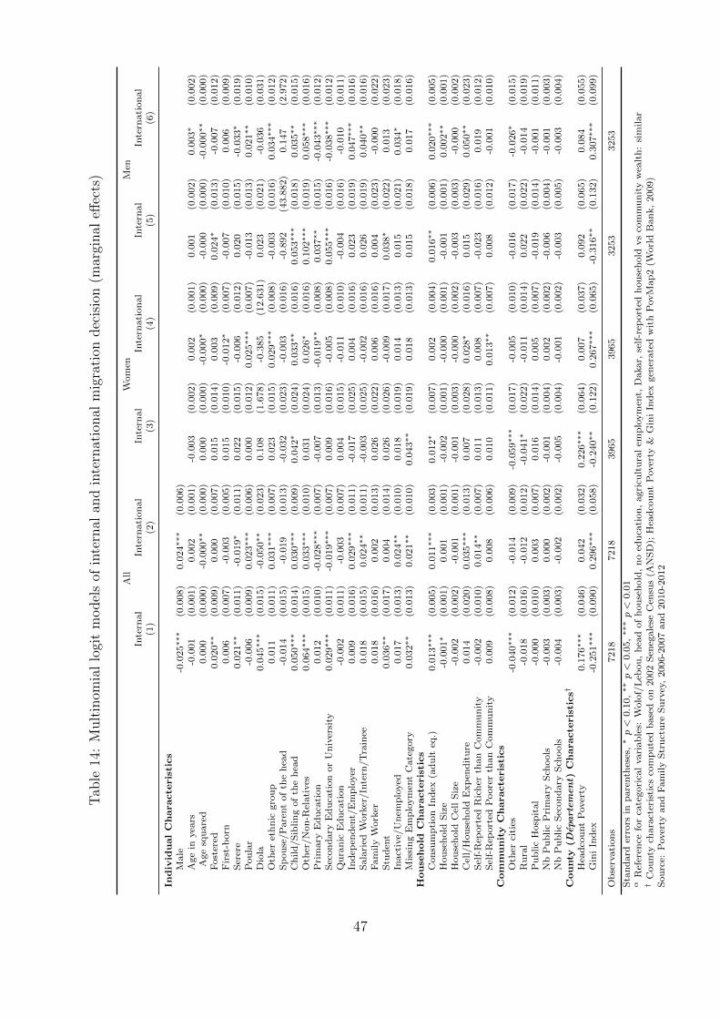
Tab

le14

:M

ult

inom

ial

logi

tm

odel

sof

inte

rnal

and

inte

rnat

ional

mig

rati

ondec

isio

n(m

argi

nal

effec

ts)

All

Wom

enM

enIn

tern

al

Inte

rnati

on

al

Inte

rnal

Inte

rnati

on

al

Inte

rnal

Inte

rnati

on

al

(1)

(2)

(3)

(4)

(5)

(6)

Individ

ualCharacte

ristics

Male

-0.0

25∗∗∗

(0.0

08)

0.0

24∗∗∗

(0.0

06)

Age

inyea

rs-0

.001

(0.0

01)

0.0

02

(0.0

01)

-0.0

03

(0.0

02)

0.0

02

(0.0

01)

0.0

01

(0.0

02)

0.0

03∗

(0.0

02)

Age

squ

are

d0.0

00

(0.0

00)

-0.0

00∗∗

(0.0

00)

0.0

00

(0.0

00)

-0.0

00∗

(0.0

00)

-0.0

00

(0.0

00)

-0.0

00∗∗

(0.0

00)

Fost

ered

0.0

20∗∗

(0.0

09)

0.0

00

(0.0

07)

0.0

15

(0.0

14)

0.0

03

(0.0

09)

0.0

24∗

(0.0

13)

-0.0

07

(0.0

12)

Fir

st-b

orn

0.0

06

(0.0

07)

-0.0

03

(0.0

05)

0.0

15

(0.0

10)

-0.0

12∗

(0.0

07)

-0.0

07

(0.0

10)

0.0

06

(0.0

09)

Ser

ere

0.0

21∗∗

(0.0

11)

-0.0

19∗

(0.0

11)

0.0

22

(0.0

15)

-0.0

06

(0.0

12)

0.0

20

(0.0

15)

-0.0

33∗

(0.0

19)

Pou

lar

-0.0

06

(0.0

09)

0.0

23∗∗∗

(0.0

06)

0.0

00

(0.0

12)

0.0

25∗∗∗

(0.0

07)

-0.0

13

(0.0

13)

0.0

21∗∗

(0.0

10)

Dio

la0.0

45∗∗∗

(0.0

15)

-0.0

50∗∗

(0.0

23)

0.1

08

(1.6

78)

-0.3

85

(12.6

31)

0.0

23

(0.0

21)

-0.0

36

(0.0

31)

Oth

eret

hn

icgro

up

0.0

11

(0.0

11)

0.0

31∗∗∗

(0.0

07)

0.0

23

(0.0

15)

0.0

29∗∗∗

(0.0

08)

-0.0

03

(0.0

16)

0.0

34∗∗∗

(0.0

12)

Sp

ou

se/P

are

nt

of

the

hea

d-0

.014

(0.0

15)

-0.0

19

(0.0

13)

-0.0

32

(0.0

23)

-0.0

03

(0.0

16)

-0.8

92

(43.8

82)

0.1

47

(2.9

72)

Ch

ild

/S

iblin

gof

the

hea

d0.0

50∗∗∗

(0.0

14)

0.0

30∗∗∗

(0.0

09)

0.0

42∗

(0.0

24)

0.0

33∗∗

(0.0

16)

0.0

53∗∗∗

(0.0

18)

0.0

35∗∗

(0.0

15)

Oth

er/N

on

-Rel

ati

ves

0.0

64∗∗∗

(0.0

15)

0.0

33∗∗∗

(0.0

10)

0.0

31

(0.0

24)

0.0

26∗

(0.0

16)

0.1

02∗∗∗

(0.0

19)

0.0

58∗∗∗

(0.0

16)

Pri

mary

Ed

uca

tion

0.0

12

(0.0

10)

-0.0

28∗∗∗

(0.0

07)

-0.0

07

(0.0

13)

-0.0

19∗∗

(0.0

08)

0.0

37∗∗

(0.0

15)

-0.0

43∗∗∗

(0.0

12)

Sec

on

dary

Ed

uca

tion

or

Un

iver

sity

0.0

29∗∗∗

(0.0

11)

-0.0

19∗∗∗

(0.0

07)

0.0

09

(0.0

16)

-0.0

05

(0.0

08)

0.0

55∗∗∗

(0.0

16)

-0.0

38∗∗∗

(0.0

12)

Qu

ran

icE

du

cati

on

-0.0

02

(0.0

11)

-0.0

03

(0.0

07)

0.0

04

(0.0

15)

-0.0

11

(0.0

10)

-0.0

04

(0.0

16)

-0.0

10

(0.0

11)

Ind

epen

den

t/E

mp

loyer

0.0

09

(0.0

16)

0.0

29∗∗∗

(0.0

11)

-0.0

17

(0.0

25)

0.0

04

(0.0

16)

0.0

23

(0.0

19)

0.0

47∗∗∗

(0.0

16)

Sala

ried

Work

er/In

tern

/T

rain

ee0.0

18

(0.0

15)

0.0

24∗∗

(0.0

11)

-0.0

03

(0.0

25)

-0.0

02

(0.0

16)

0.0

26

(0.0

19)

0.0

40∗∗

(0.0

16)

Fam

ily

Work

er0.0

18

(0.0

16)

0.0

02

(0.0

13)

0.0

26

(0.0

22)

0.0

06

(0.0

16)

0.0

04

(0.0

23)

-0.0

00

(0.0

22)

Stu

den

t0.0

36∗∗

(0.0

17)

0.0

04

(0.0

14)

0.0

26

(0.0

26)

-0.0

09

(0.0

17)

0.0

38∗

(0.0

22)

0.0

13

(0.0

23)

Inact

ive/

Un

emp

loyed

0.0

17

(0.0

13)

0.0

24∗∗

(0.0

10)

0.0

18

(0.0

19)

0.0

14

(0.0

13)

0.0

15

(0.0

21)

0.0

34∗

(0.0

18)

Mis

sin

gE

mp

loym

ent

Cate

gory

0.0

32∗∗

(0.0

13)

0.0

21∗∗

(0.0

10)

0.0

43∗∗

(0.0

19)

0.0

18

(0.0

13)

0.0

15

(0.0

18)

0.0

17

(0.0

16)

House

hold

Characte

ristics

Con

sum

pti

on

Ind

ex(a

du

lteq

.)0.0

13∗∗∗

(0.0

05)

0.0

11∗∗∗

(0.0

03)

0.0

12∗

(0.0

07)

0.0

02

(0.0

04)

0.0

16∗∗

(0.0

06)

0.0

20∗∗∗

(0.0

05)

Hou

seh

old

Siz

e-0

.001∗

(0.0

01)

0.0

01

(0.0

01)

-0.0

02

(0.0

01)

-0.0

00

(0.0

01)

-0.0

01

(0.0

01)

0.0

02∗∗

(0.0

01)

Hou

seh

old

Cel

lS

ize

-0.0

02

(0.0

02)

-0.0

01

(0.0

01)

-0.0

01

(0.0

03)

-0.0

00

(0.0

02)

-0.0

03

(0.0

03)

-0.0

00

(0.0

02)

Cel

l/H

ou

seh

old

Exp

end

itu

re0.0

14

(0.0

20)

0.0

35∗∗∗

(0.0

13)

0.0

07

(0.0

28)

0.0

28∗

(0.0

16)

0.0

15

(0.0

29)

0.0

50∗∗

(0.0

23)

Sel

f-R

eport

edR

ich

erth

an

Com

mu

nit

y-0

.002

(0.0

10)

0.0

14∗∗

(0.0

07)

0.0

11

(0.0

13)

0.0

08

(0.0

07)

-0.0

23

(0.0

16)

0.0

19

(0.0

12)

Sel

f-R

eport

edP

oore

rth

an

Com

mu

nit

y0.0

09

(0.0

08)

0.0

08

(0.0

06)

0.0

10

(0.0

11)

0.0

13∗∗

(0.0

07)

0.0

08

(0.0

12)

-0.0

01

(0.0

10)

Com

munity

Characte

ristics

Oth

erci

ties

-0.0

40∗∗∗

(0.0

12)

-0.0

14

(0.0

09)

-0.0

59∗∗∗

(0.0

17)

-0.0

05

(0.0

10)

-0.0

16

(0.0

17)

-0.0

26∗

(0.0

15)

Ru

ral

-0.0

18

(0.0

16)

-0.0

12

(0.0

12)

-0.0

41∗

(0.0

22)

-0.0

11

(0.0

14)

0.0

22

(0.0

22)

-0.0

14

(0.0

19)

Pu

blic

Hosp

ital

-0.0

00

(0.0

10)

0.0

03

(0.0

07)

0.0

16

(0.0

14)

0.0

05

(0.0

07)

-0.0

19

(0.0

14)

-0.0

01

(0.0

11)

Nb

Pu

blic

Pri

mary

Sch

ools

-0.0

03

(0.0

03)

0.0

00

(0.0

02)

-0.0

01

(0.0

04)

0.0

02

(0.0

02)

-0.0

06

(0.0

04)

-0.0

01

(0.0

03)

Nb

Pu

blic

Sec

on

dary

Sch

ools

-0.0

04

(0.0

03)

-0.0

02

(0.0

02)

-0.0

05

(0.0

04)

-0.0

01

(0.0

02)

-0.0

03

(0.0

05)

-0.0

03

(0.0

04)

County

(Depart

em

en

t)Characte

ristics†

Hea

dco

unt

Pover

ty0.1

76∗∗∗

(0.0

46)

0.0

42

(0.0

32)

0.2

26∗∗∗

(0.0

64)

0.0

07

(0.0

37)

0.0

92

(0.0

65)

0.0

84

(0.0

55)

Gin

iIn

dex

-0.2

51∗∗∗

(0.0

90)

0.2

96∗∗∗

(0.0

58)

-0.2

40∗∗

(0.1

22)

0.2

67∗∗∗

(0.0

65)

-0.3

16∗∗

(0.1

32)

0.3

07∗∗∗

(0.0

99)

Ob

serv

ati

on

s7218

7218

3965

3965

3253

3253

Sta

nd

ard

erro

rsin

pare

nth

eses

,∗p<

0.1

0,∗∗p<

0.0

5,∗∗∗p<

0.0

1α

Ref

eren

cefo

rca

tegori

cal

vari

ab

les:

Wolo

f/L

ebou

,h

ead

of

hou

seh

old

,n

oed

uca

tion

,agri

cult

ura

lem

plo

ym

ent,

Dakar,

self

-rep

ort

edh

ou

seh

old

vs

com

mu

nit

yw

ealt

h:

sim

ilar

†C

ou

nty

chara

cter

isti

csco

mp

ute

db

ase

don

2002

Sen

egale

seC

ensu

s(A

NS

D);

Hea

dco

unt

Pover

ty&

Gin

iIn

dex

gen

erate

dw

ith

PovM

ap

2(W

orl

dB

an

k,

2009)

Sou

rce:

Pover

tyan

dF

am

ily

Str

uct

ure

Su

rvey

,2006-2

007

an

d2010-2

012

47

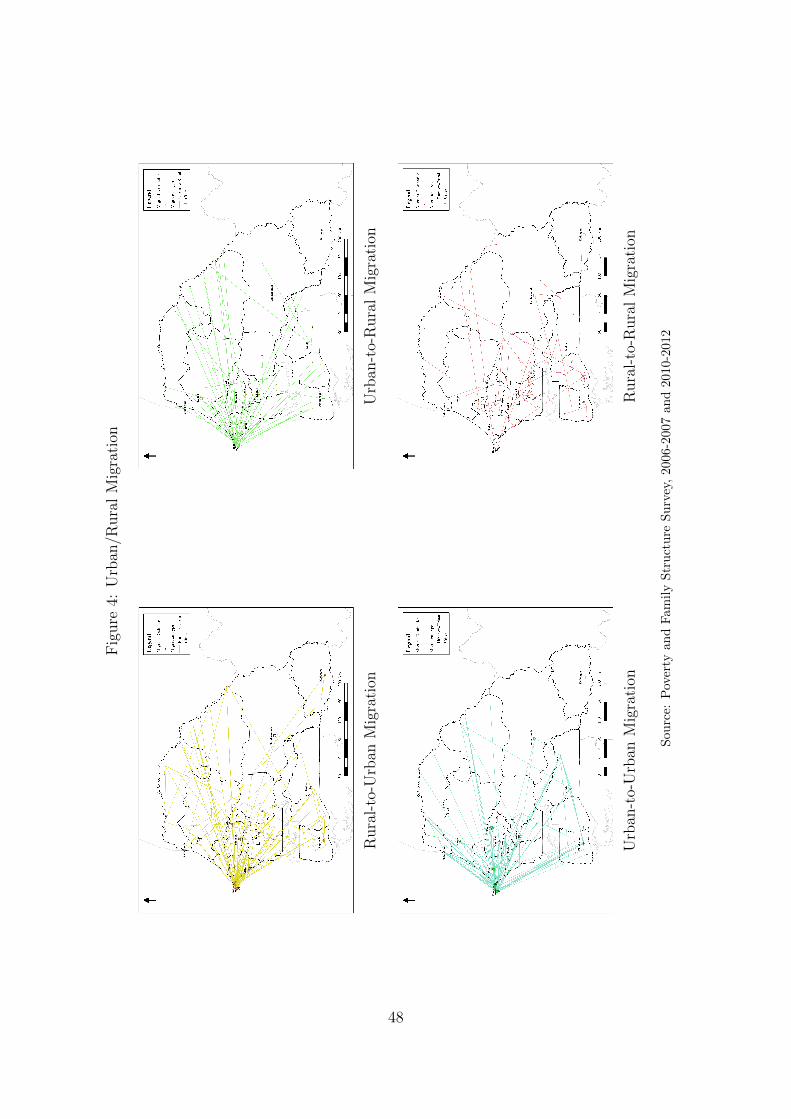
Fig

ure

4:U

rban

/Rura

lM

igra

tion

Rura

l-to

-Urb

anM

igra

tion

Urb

an-t

o-R

ura

lM

igra

tion

Urb

an-t

o-U

rban

Mig

rati

onR

ura

l-to

-Rura

lM

igra

tion

Sou

rce:

Pov

erty

an

dF

am

ily

Str

uct

ure

Su

rvey

,2006-2

007

and

2010-2

012

48

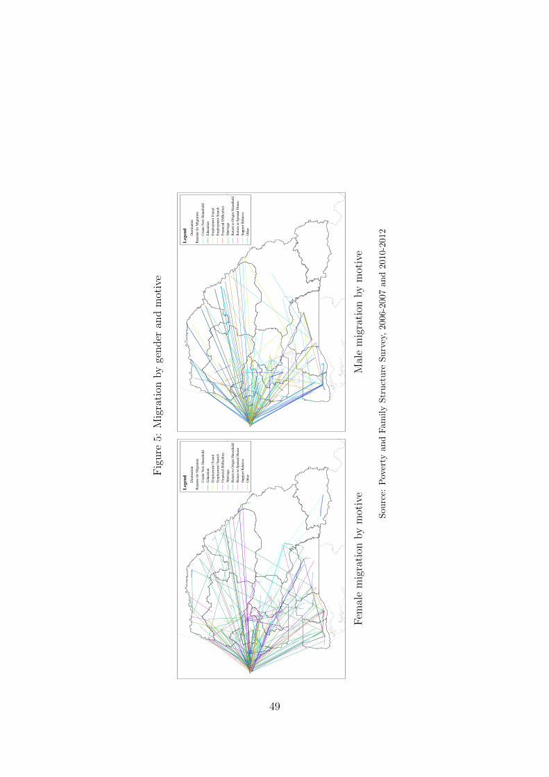
Fig

ure

5:M

igra

tion

by

gender

and

mot

ive

Des

tinat

ion

Reas

ons f

or M

igra

tion

Crea

te N

ew H

ouse

hold

Educ

atio

nEm

ploy

men

t Fou

ndEm

ploy

men

t Sea

rch

Fina

ncia

l Diff

icul

ties

Mar

riage

Retu

rn to

Orig

in H

ouse

hold

Retu

rn to

Spo

usal

Hou

seSu

ppor

t Rel

ativ

eO

ther

Legend

Fem

ale

mig

rati

onby

mot

ive

Des

tinat

ion

Reas

ons f

or M

igra

tion

Crea

te N

ew H

ouse

hold

Educ

atio

nEm

ploy

men

t Fou

ndEm

ploy

men

t Sea

rch

Fina

ncia

l Diff

icul

ties

Mar

riage

Retu

rn to

Orig

in H

ouse

hold

Retu

rn to

Spo

usal

Hou

seSu

ppor

t Rel

ativ

eO

ther

Legend

Mal

em

igra

tion

by

mot

ive

Sou

rce:

Pov

erty

an

dF

am

ily

Str

uct

ure

Su

rvey

,2006-2

007

and

2010-2

012

49

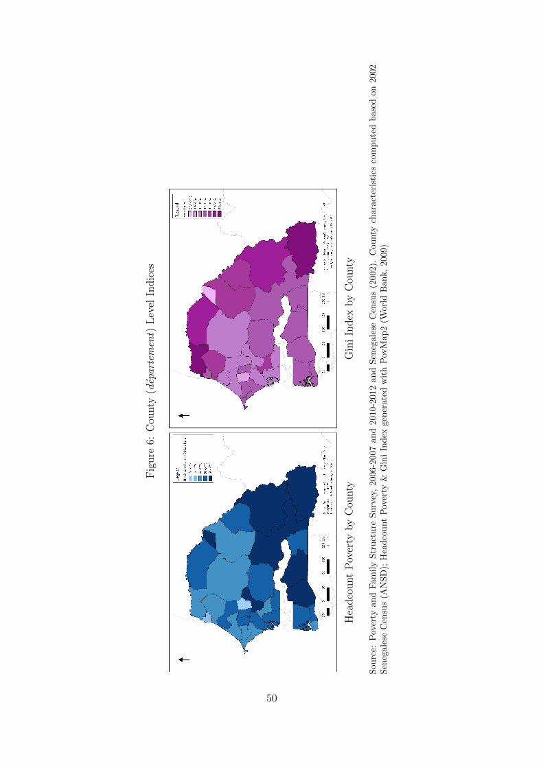
Fig

ure

6:C

ounty

(dep

arte

men

t)L

evel

Indic

es

Hea

dco

unt

Pov

erty

by

Cou

nty

Gin

iIn

dex

by

Cou

nty

Sou

rce:

Pov

erty

and

Fam

ily

Str

uct

ure

Su

rvey

,20

06-2

007

an

d2010-2

012

an

dS

eneg

ale

seC

ensu

s(2

002).

Cou

nty

chara

cter

isti

csco

mp

ute

db

ase

don

2002

Sen

egal

ese

Cen

sus

(AN

SD

);H

ead

cou

nt

Pov

erty

&G

ini

Ind

exgen

erate

dw

ith

Pov

Map

2(W

orl

dB

an

k,

2009)

50