Gene Features Selection for Three-Class Disease

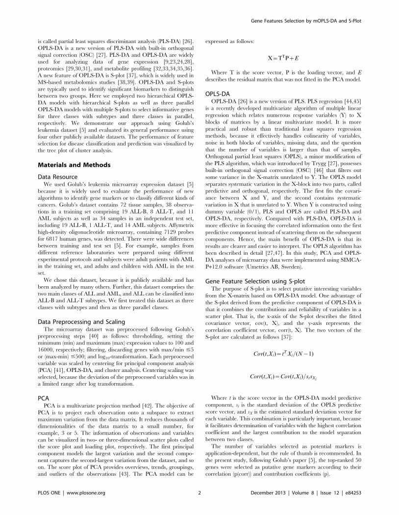
Gene Features Selection for Three-Class DiseaseClassification via Multiple Orthogonal Partial LeastSquare Discriminant Analysis and S-Plot UsingMicroarray DataMingxing Yang1,3, Xiumin Li1, Zhibin Li1, Zhimin Ou1, Ming Liu1, Suhuan Liu1, Xuejun Li1,2*,

Shuyu Yang1*

1 Xiamen Diabetes Institute, the First Affiliated Hospital of Xiamen University, Xiamen, China, 2 Department of Endocrinology and Diabetes, the First Affiliated Hospital of

Xiamen University, Xiamen, China, 3 Department of Electronic Science, School of Physics and Mechanical & Electrical Engineering, Xiamen University, Xiamen, China

Abstract

Motivation: DNA microarray analysis is characterized by obtaining a large number of gene variables from a small number ofobservations. Cluster analysis is widely used to analyze DNA microarray data to make classification and diagnosis of disease.Because there are so many irrelevant and insignificant genes in a dataset, a feature selection approach must be employed indata analysis. The performance of cluster analysis of this high-throughput data depends on whether the feature selectionapproach chooses the most relevant genes associated with disease classes.

Results: Here we proposed a new method using multiple Orthogonal Partial Least Squares-Discriminant Analysis (mOPLS-DA) models and S-plots to select the most relevant genes to conduct three-class disease classification and prediction. Wetested our method using Golub’s leukemia microarray data. For three classes with subtypes, we proposed hierarchicalorthogonal partial least squares-discriminant analysis (OPLS-DA) models and S-plots to select features for two main classesand their subtypes. For three classes in parallel, we employed three OPLS-DA models and S-plots to choose marker genesfor each class. The power of feature selection to classify and predict three-class disease was evaluated using cluster analysis.Further, the general performance of our method was tested using four public datasets and compared with those of fourother feature selection methods. The results revealed that our method effectively selected the most relevant features fordisease classification and prediction, and its performance was better than that of the other methods.

Citation: Yang M, Li X, Li Z, Ou Z, Liu M, et al. (2013) Gene Features Selection for Three-Class Disease Classification via Multiple Orthogonal Partial Least SquareDiscriminant Analysis and S-Plot Using Microarray Data. PLoS ONE 8(12): e84253. doi:10.1371/journal.pone.0084253

Editor: Vladimir B. Bajic, King Abdullah University of Science and Technology, Saudi Arabia

Received May 3, 2013; Accepted November 12, 2013; Published December 30, 2013

Copyright: � 2013 Yang et al. This is an open-access article distributed under the terms of the Creative Commons Attribution License, which permitsunrestricted use, distribution, and reproduction in any medium, provided the original author and source are credited.

Funding: This work was supported by Xiamen Science and Technology Bureau (Xiamen Research Platform for Systems Biology of MetabolicDisease,3502Z20100001), National Natural Science Foundation to Shuyu Yang (30973912), Xuejun Li (81073113) and Suhuan Liu (81270901). The funders hadno role in study design, data collection, and analysis, decision to publish, or preparation of the menuscript.

Competing Interests: The authors have declared that no competing interests exist.

* E-mail: [email protected] (SY); [email protected] (Xuejun Li)

Introduction

DNA microarray analysis is an important tool in medicine and

life sciences, because it measures simultaneously the expression

levels of thousands of genes. In the past few years, many

multivariate data analysis methods have been developed and

applied to extract the full potential from microarray experiments

including cluster analysis [1,2], support vector machine (SVM)

[3,4], self-organizing maps (SOMs) [5,6], artificial neural networks

(ANN) [7,8], partial least squares (PLS) [9], and non-negative

matrix factorization (NMF) [10,11,12,13,14]. Cluster analysis may

be the most widely used method because, at least in part, it not

only generates an intuitive tree to visualize clusters, and as an

unsupervised technique, clusters samples and genes into different

groups.

Microarray data typically consist of a relatively small sample

size (usually several dozens) and a large number of genes (several

thousands), most of which may be irrelevant, insignificant, or

redundant for disease classification and prediction [15,16].

Therefore, many gene-selection approaches for cluster analysis

have been proposed such as signal to noise ratio (S2N) [5], ANN

[7], Kruskal-Wallis nonparametric one-way ANOVA (KW) [17],

ratio of genes between-categories to within-category sums of

squares (BW) [18], nonparametric test [19], t-test [20,21], genetic

algorithm (GA), and k-nearest neighbor (GA/KNN) [22]. Many

approaches were aimed to deal with two-class gene selection

problems, and only a few studies involved multiclass gene selection

(three classes or more) and classification for cluster analysis.

In this study, we describe the development of a novel multiple

orthogonal partial least squares discriminant analysis (mOPLS-

DA) model and S-plots to conduct three-class gene selection.

Partial least squares (PLS), a well-known dimension-reduction

method, is a simple and efficient algorithm that conducts two-class

and multiclass classification [9,23] and predicts clinical outcome

[24] and survival times [25] using gene expression microarray

data. When the response is dummy variable (0/1), the PLS model

PLOS ONE | www.plosone.org 1 December 2013 | Volume 8 | Issue 12 | e84253

is called partial least squares discriminant analysis (PLS-DA) [26].

OPLS-DA is a new version of PLS-DA with built-in orthogonal

signal correction (OSC) [27]. PLS-DA and OPLS-DA are widely

used for analyzing data of gene expression [9,23,24,28],

proteomics [29,30,31], and metabolite profiling [32,33,34,35,36].

A new feature of OPLS-DA is S-plot [37], which is widely used in

MS-based metabolomics studies [38,39]. OPLS-DA and S-plots

are typically used to identify significant biomarkers to distinguish

between two groups. Here we employed two hierarchical OPLS-

DA models with hierarchical S-plots as well as three parallel

OPLS-DA models with multiple S-plots to select informative genes

for three classes with subtypes and three classes in parallel,

respectively. We demonstrate our approach using Golub’s

leukemia dataset [5] and evaluated its general performance using

four other publicly available datasets. The performance of feature

selection for disease classification and prediction was visualized by

the tree plot of cluster analysis.

Materials and Methods

Data ResourceWe used Golub’s leukemia microarray expression dataset [5]

because it is widely used to evaluate the performance of new

algorithms to identify gene markers or to classify different kinds of

cancers. Golub’s dataset contains 72 tissue samples, 38 observa-

tions in a training set comprising 19 ALL-B, 8 ALL-T, and 11

AML subjects as well as 34 samples in an independent test set,

including 19 ALL-B, 1 ALL-T, and 14 AML subjects. Affymetrix

high-density oligonucleotide microarray, containing 7129 probes

for 6817 human genes, was detected. There were wide differences

between training and test set [5]. For example, samples from

different reference laboratories were prepared using different

experimental protocols and subjects were adult patients with AML

in the training set, and adults and children with AML in the test

set.

We chose this dataset, because it is publicly available and has

been analyzed by many others. Further, this dataset comprises the

two main classes of ALL and AML, and ALL can be classified into

ALL-B and ALL-T subtypes. We first treated this dataset as three

classes with subtypes and then as three parallel classes.

Data Preprocessing and ScalingThe microarray dataset was preprocessed following Golub’s

preprocessing steps [40] as follows: thresholding, setting the

minimum (min) and maximum (max) expression values to 100 and

16000, respectively; filtering, discarding genes with max/min #5

or (max-min) #500; and log10-transformation. Each preprocessed

variable was scaled by centering for principal component analysis

(PCA) [41], OPLS-DA, and cluster analysis. Centering scaling was

selected, because the deviation of the preprocessed variables was in

a limited range after log transformation.

PCAPCA is a multivariate projection method [42]. The objective of

PCA is to project each observation onto a subspace to extract

maximum variation from the data matrix. It reduces thousands of

dimensionalities of the data matrix to a small number, for

example, 3 or 5. The information of observations and variables

can be visualized in two- or three-dimensional scatter plots called

the score plot and loading plot, respectively. The first principal

component models the largest variation and the second compo-

nent captures the second-largest variation from the dataset, and so

on. The score plot of PCA provides overviews, trends, groupings,

and outliers of the observations [43]. The PCA model can be

expressed as follows:

X~TTPzE

Where T is the score vector, P is the loading vector, and E

describes the residual matrix that was not fitted in the PCA model.

OPLS-DAOPLS-DA [26] is a new version of PLS. PLS regression [44,45]

is a recently developed multivariate algorithm of multiple linear

regression which relates numerous response variables (Y) to X

blocks of matrices by a linear multivariate model. It is more

practical and robust than traditional least squares regression

methods, because it effectively handles colinearity of variables,

noise in both blocks of variables, missing data, and the question

that the number of variables is larger than that of samples.

Orthogonal partial least squares (OPLS), a minor modification of

the PLS algorithm, which was introduced by Trygg [27], possesses

built-in orthogonal signal correction (OSC) [46] that filters out

some variance in the X-matrix unrelated to Y. The OPLS model

separates systematic variation in the X-block into two parts, called

predictive and orthogonal, respectively. The first fits the covari-

ance between X and Y, and the second contains systematic

variation in X that is unrelated to Y. When Y is constructed using

dummy variable (0/1), PLS and OPLS are called PLS-DA and

OPLS-DA, respectively. Compared with PLS-DA, OPLS-DA is

more effective in focusing the correlated information onto the first

predictive component instead of scattering them on the subsequent

components. Hence, the main benefit of OPLS-DA is that its

results are clearer and easier to interpret. The OPLS algorithm has

been described in detail [27,47]. In this study, PCA and OPLS-

DA analyses of microarray data were implemented using SIMCA-

P+12.0 software (Umetrics AB, Sweden).

Gene Feature Selection using S-plotThe purpose of S-plot is to select putative interesting variables

from the X-matrix based on OPLS-DA model. One advantage of

the S-plot derived from the predictive component of OPLS-DA is

that it combines the contributions and reliability of variables in a

scatter plot. That is, the x-axis of the S-plot describes the fitted

covariance vector, cov(t, X), and the y-axis represents the

correlation coefficient vector, corr(t, X). The two vectors of the

S-plot are calculated as follows [37]:

Cov(t,Xi)~tT Xi=(N{1)

Corr(t,Xi)~Cov(t,Xi)=stsXi

Where t is the score vector in the OPLS-DA model predictive

component, st is the standard deviation of the OPLS predictive

score vector, and sX is the estimated standard deviation vector for

each variable. This combination is particularly important, because

it facilitates determination of variables with the highest correlation

coefficient and the largest contribution to the model separation

between two classes.

The number of variables selected as potential markers is

application-dependent, but the rule of thumb is recommended. In

the present study, following Golub’s paper [5], the top-ranked 50

genes were selected as putative gene markers according to their

correlation (p(corr)) and contribution coefficients (p).

Gene Features Selection by mOPLS-DA and S-Plot


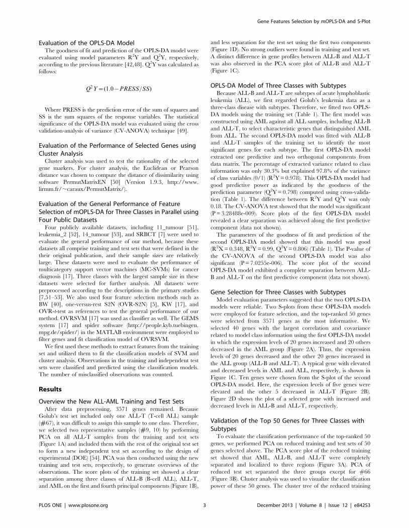
Evaluation of the OPLS-DA ModelThe goodness of fit and prediction of the OPLS-DA model were

evaluated using model parameters R2Y and Q2Y, respectively,

according to the previous literature [42,48]. Q2Y was calculated as

follows:

Q2Y~(1:0{PRESS=SS)

Where PRESS is the prediction error of the sum of squares and

SS is the sum squares of the response variables. The statistical

significance of the OPLS-DA model was evaluated using the cross

validation-analysis of variance (CV-ANOVA) technique [49].

Evaluation of the Performance of Selected Genes usingCluster Analysis

Cluster analysis was used to test the rationality of the selected

gene markers. For cluster analysis, the Euclidean or Pearson

distance was chosen to compute the distance of dissimilarity using

software PermutMatrixEN [50] (Version 1.9.3, http://www.

lirmm.fr/,caraux/PermutMatrix/).

Evaluation of the General Performance of FeatureSelection of mOPLS-DA for Three Classes in Parallel usingFour Public Datasets

Four publicly available datasets, including 11_tumour [51],

leukemia_2 [52], 14_tumour [53], and SRBCT [7] were used to

evaluate the general performance of our method, because these

datasets all comprise training and test sets that were defined in the

their original publication, and their sample sizes are relatively

large. These datasets were used to evaluate the performance of

multicategory support vector machines (MC-SVMs) for cancer

diagnosis [17]. Three classes with the largest sample size in these

datasets were selected for further analysis. All datasets were

preprocessed according to the descriptions in the primary studies

[7,51–53]. We also used four feature selection methods such as

BW [40], one-versus-rest S2N (OVR-S2N) [5], KW [17], and

OVR-t-test as references to test the general performance of our

method. OVRSVM [17] was used as classifier as well. The GEMS

system [17] and spider software (http://people.kyb.tuebingen.

mpg.de/spider/) in the MATLAB environment were employed to

filter genes and fit classification model of OVRSVM.

We first used these methods to extract features from the training

set and utilized them to fit the classification models of SVM and

cluster analysis. Observations in the training and independent test

sets were classified and predicted using the classification models.

The number of misclassified observations was counted.

Results

Overview the New ALL-AML Training and Test SetsAfter data preprocessing, 3571 genes remained. Because

Golub’s test set included only one ALL-T (T-cell ALL) sample

(#67), it was difficult to assign this sample to one class. Therefore,

we selected two representative samples (#9, 10) by performing

PCA on all ALL-T samples from the training and test sets

(Figure 1A) and included them with the rest of the original test set

to form a new independent test set according to the design of

experimental (DOE) [54]. PCA was then conducted using the new

training and test sets, respectively, to generate overviews of the

observations. The score plots of the training set showed a clear

separation among three classes of ALL-B (B-cell ALL), ALL-T,

and AML on the first and fourth principal components (Figure 1B),

and less separation for the test set using the first two components

(Figure 1D). No strong outliers were found in training and test set.

A distinct difference in gene profiles between ALL-B and ALL-T

was also observed in the PCA score plot of ALL-B and ALL-T

(Figure 1C).

OPLS-DA Model of Three Classes with SubtypesBecause ALL-B and ALL-T are subtypes of acute lymphoblastic

leukemia (ALL), we first regarded Golub’s leukemia data as a

three-class disease with subtypes. Therefore, we fitted two OPLS-

DA models using the training set (Table 1). The first model was

constructed using AML against all ALL samples, including ALL-B

and ALL-T, to select characteristic genes that distinguished AML

from ALL. The second OPLS-DA model was fitted with ALL-B

and ALL-T samples of the training set to identify the most

significant genes for each subtype. The first OPLS-DA model

extracted one predictive and two orthogonal components from

data matrix. The percentage of extracted variance related to class

information was only 30.3% but explained 97.8% of the variance

of class variables (0/1) (R2Y = 0.978). This OPLS-DA model had

good predictive power as indicated by the goodness of the

prediction parameter (Q2Y = 0.798) computed using cross-valida-

tion (Table 1). The difference between R2Y and Q2Y was only

0.18. The CV-ANOVA test showed that the model was significant

(P = 3.28488e-009). Score plots of the first OPLS-DA model

revealed a clear separation was achieved along the first predictive

component (data not shown).

The parameters of the goodness of fit and prediction of the

second OPLS-DA model showed that this model was good

(R2X = 0.348, R2Y = 0.99, Q2Y = 0.806) (Table 1). The P-value of

the CV-ANOVA of the second OPLS-DA model was also

significant (P = 7.0255e-006). The score plot of the second

OPLS-DA model exhibited a complete separation between ALL-

B and ALL-T on the first predictive component (data not shown).

Gene Selection for Three Classes with SubtypesModel evaluation parameters suggested that the two OPLS-DA

models were reliable. Two S-plots from these OPLS-DA models

were employed for feature selection, and the top-ranked 50 genes

were selected from 3571 genes as the most informative. We

selected 40 genes with the largest correlation and covariance

related to model class information using the first OPLS-DA model

in which the expression levels of 20 genes increased and 20 others

decreased in the AML group (Figure 2A). Thus, the expression

levels of 20 genes decreased and the other 20 genes increased in

the ALL group (ALL-B and ALL-T). A typical gene with elevated

and decreased levels in AML and ALL, respectively, is shown in

Figure 1C. Ten genes were chosen from the S-plot of the second

OPLS-DA model. Here, the expression levels of five genes were

elevated and the other 5 decreased in ALL-T (Figure 2B).

Figure 2D shows the plot of a selected gene with increased and

decreased levels in ALL-B and ALL-T, respectively.

Validation of the Top 50 Genes for Three Classes withSubtypes

To evaluate the classification performance of the top-ranked 50

genes, we performed PCA on reduced training and test sets of 50

genes selected above. The PCA score plot of the reduced training

set showed that AML, ALL-B, and ALL-T were completely

separated and localized to three regions (Figure 3A). PCA of

reduced test set separated the three groups except for #66

(Figure 3B). Cluster analysis was used to visualize the classification

power of these 50 genes. The cluster tree of the reduced training



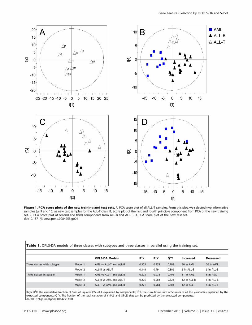
Figure 1. PCA score plots of the new training and test sets. A, PCA score plot of all ALL-T samples. From this plot, we selected two informativesamples (# 9 and 10) as new test samples for the ALL-T class. B, Score plot of the first and fourth principle component from PCA of the new trainingset. C, PCA score plot of second and third components from ALL-B and ALL-T. D, PCA score plot of the new test set.doi:10.1371/journal.pone.0084253.g001

Table 1. OPLS-DA models of three classes with subtypes and three classes in parallel using the training set.

OPLS-DA Models R2X R2Y Q2Y Increased Decreased

Three classes with subtype Model 1 AML vs ALL-T and ALL-B 0.303 0.978 0.798 20 in AML 20 in AML

Model 2 ALL-B vs ALL-T 0.348 0.99 0.806 5 in ALL-B 5 in ALL-B

Three classes in parallel Model 1 AML vs ALL-T and ALL-B 0.303 0.978 0.798 11 in AML 6 in AML

Model 2 ALL-B vs AML and ALL-T 0.275 0.984 0.823 12 in ALL-B 5 in ALL-B

Model 3 ALL-T vs AML and ALL-B 0.271 0.983 0.804 12 in ALL-T 5 in ALL-T

Keys: R2X, the cumulative fraction of Sum of Squares (SS) of X explained by components; R2Y, the cumulative Sum of Squares of all the y-variables explained by theextracted components; Q2Y, The fraction of the total variation of Y (PLS and OPLS) that can be predicted by the extracted components.doi:10.1371/journal.pone.0084253.t001



set showed that all samples were correctly classified (Figure 3E).

Notably, the subtypes of ALL-B and ALL-T were also accurately

classified (Figure 3E). Although we selected the best results of

clustering for the training set with 3571 genes, one AML sample

was misclassified into the ALL-B group (#29) and ALL was

misclassified into three subclasses (Figure 3C).

The results of cluster analysis showed that the classification

performance of the test set comprised of top 50 genes was

excellent, because only one sample was misclassified (#66)

(Figure 3F). This sample was incorrectly assigned to the ALL

group by Golub [5] and other researchers [9,55,56]. Moreover,

two ALL-T samples (#9, 10) were grouped together in one class

and parallel with the ALL-B group (Figure 3F). With the 3571

gene dataset, AML and ALL were not clearly distinguished, and

two ALL-T samples were incorrectly predicted as ALL-B together

with the AML samples (Figure 3D).

Feature Selection for Three Parallel ClassesWe next considered AML, ALL-B, and ALL-T as three parallel

classes without subtypes to select characteristic genes for classifying

disease. Therefore, we selected features for each class through the

corresponding OPLS-DA models and S-plots. Three OPLS-DA

models were fitted using training set of AML vs. ALL-B and ALL-

T, ALL-B vs. AML and ALL-T, and ALL-T vs. AML and ALL-B

(Table 1). The parameters of model evaluation showed that these

three models were very good in the goodness of fit and prediction

(Table 1). Score plots of each OPLS-DA model demonstrated that

each group was clearly separated from the others on the first

predictive component. Figure 4A is the score plot from OPLS-DA

model of ALL-B vs. AML and ALL-T which shows that ALL-B is

distinct from AML and ALL-T, and more interestingly, AML is

separated from ALL-T on the first orthogonal component.

Seventeen top genes were selected from each OPLS-DA model

using the S-plot (Figure 4B, C, D). The number of genes selected

from each model and the model parameters are shown in Table 1.

Note that feature selection depended mainly on the correlation

between gene variables and the predictive scores p(corr) and that

the genes with a larger contribution were preferred when there

was no significant difference in the correlation between two genes.

Among them, gene M27891 was chosen twice. Hence, only the

top-ranked 50 genes were selected and analyzed further. We next

performed PCA on the training and test sets with the new top-

ranked 50 genes. The PCA score plot of the training set showed

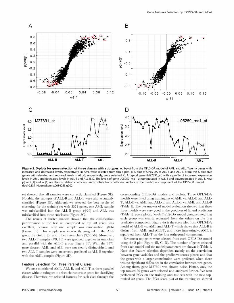
Figure 2. S-plots for gene selection of three classes with subtypes. A, S-plot from the OPLS-DA model of AML and ALL. Twenty genes withincreased and decreased levels, respectively, in AML were selected from this S-plot. B, S-plot of OPLS-DA of ALL-B and ALL-T. From this S-plot, fivegenes with elevated and reduced levels in ALL-B, respectively, were selected. C, A typical gene (M27891_at) with a profile of increased expressionlevels in AML and decreased levels in ALL-T and ALL-B. D, The levels of gene U05259_rna1_at upregulated in ALL-B and downregulated in ALL-T. Key:p(corr) [1] and w [1] are the correlation coefficient and contribution coefficient vectors of the predictive component of the OPLS-DA model.doi:10.1371/journal.pone.0084253.g002



that three classes clustered in three distinct regions except one

sample (#17), which was in the joint region (Figure 4E), and the

score plot of the test set showed that three classes were clearly

located in three regions of the score plot with an unknown-class

sample (#66) (Figure 4F).

The Classification Power of the Top 50 Genes for ThreeParallel Classes

To examine the rationality of the top 50 genes, we next

performed cluster analysis on the training and test sets, respec-

tively, using the Euclidean distance and complete linkage. The

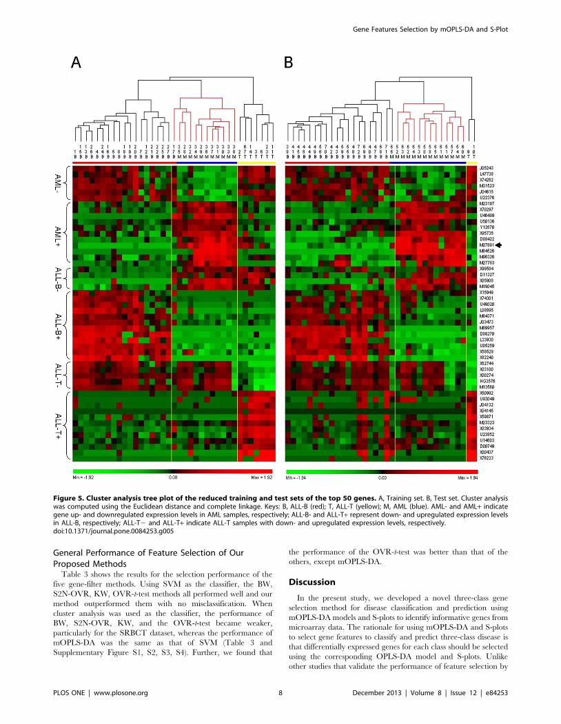
cluster tree for the training set of the new top 50 genes showed that

all samples were assigned accurately into ALL-T, ALL-B, and

AML, except for one sample (#17), which belongs to the ALL-B

group but was incorrectly classified as AML (Figure 5A). We found

that when we separated all training samples into two classes, these

two clusters were ALL-T vs. ALL-B and AML other than AML vs.

ALL-B and ALL-T. Similarly, all test set samples clustered into

three distinct classes in a profile similar to that of the training set

with one misclassified sample (#66). There were only two samples

in the ALL-T group of the test set (#9, 10). However, these two

samples still clustered into one class in parallel with ALL-B and

AML (Figure 5B). The gene features identified by each model were

displayed in a color-coded data matrix in Figure 5A and B, and

there was no difference in the gene expression profile between

training and test sets.

Comparison of the Classification Performance with t-testTo assess the performance of our approach, we compared the

classification power of mOPLS-DA with that of t-test using

Golub’s dataset. The OVR-t-test was employed to select significant

features for each class. Selection methods were described in

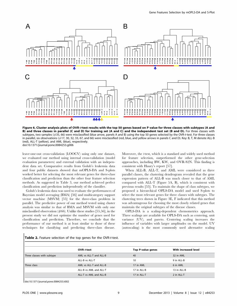
Table 2. For three classes with subtypes, one sample each from the

training and test sets was misclassified (Figure 6A and B).

Unfortunately, there were six misclassified observations (five from

the training set and one from test set) for three classes in parallel

(Figure 6C and D).

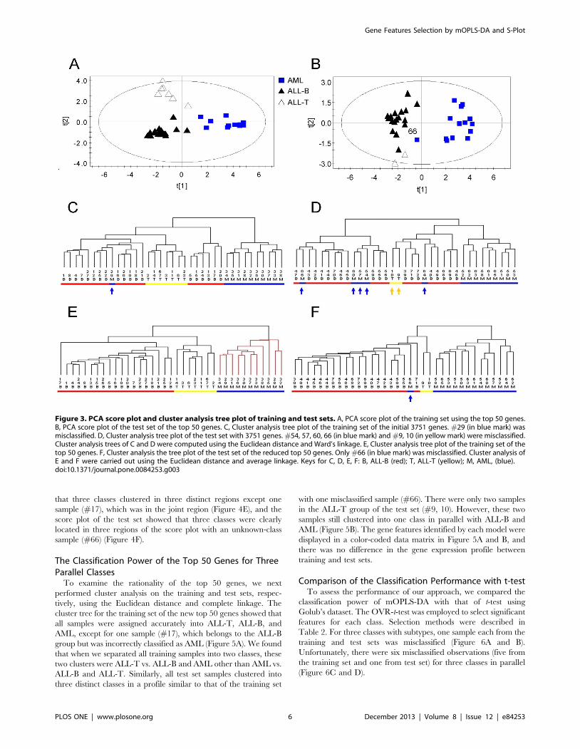
Figure 3. PCA score plot and cluster analysis tree plot of training and test sets. A, PCA score plot of the training set using the top 50 genes.B, PCA score plot of the test set of the top 50 genes. C, Cluster analysis tree plot of the training set of the initial 3751 genes. #29 (in blue mark) wasmisclassified. D, Cluster analysis tree plot of the test set with 3751 genes. #54, 57, 60, 66 (in blue mark) and #9, 10 (in yellow mark) were misclassified.Cluster analysis trees of C and D were computed using the Euclidean distance and Ward’s linkage. E, Cluster analysis tree plot of the training set of thetop 50 genes. F, Cluster analysis the tree plot of the test set of the reduced top 50 genes. Only #66 (in blue mark) was misclassified. Cluster analysis ofE and F were carried out using the Euclidean distance and average linkage. Keys for C, D, E, F: B, ALL-B (red); T, ALL-T (yellow); M, AML, (blue).doi:10.1371/journal.pone.0084253.g003



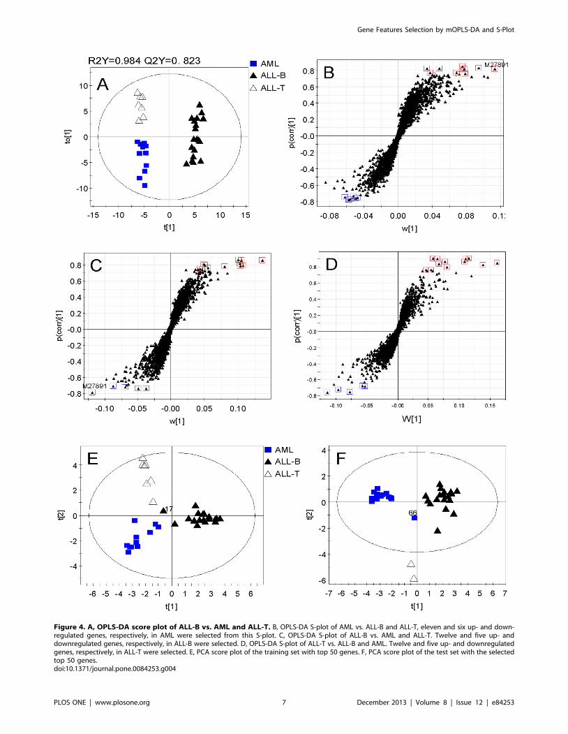
Figure 4. A, OPLS-DA score plot of ALL-B vs. AML and ALL-T. B, OPLS-DA S-plot of AML vs. ALL-B and ALL-T, eleven and six up- and down-regulated genes, respectively, in AML were selected from this S-plot. C, OPLS-DA S-plot of ALL-B vs. AML and ALL-T. Twelve and five up- anddownregulated genes, respectively, in ALL-B were selected. D, OPLS-DA S-plot of ALL-T vs. ALL-B and AML. Twelve and five up- and downregulatedgenes, respectively, in ALL-T were selected. E, PCA score plot of the training set with top 50 genes. F, PCA score plot of the test set with the selectedtop 50 genes.doi:10.1371/journal.pone.0084253.g004



General Performance of Feature Selection of OurProposed Methods

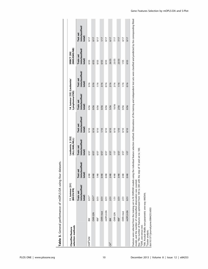
Table 3 shows the results for the selection performance of the

five gene-filter methods. Using SVM as the classifier, the BW,

S2N-OVR, KW, OVR-t-test methods all performed well and our

method outperformed them with no misclassification. When

cluster analysis was used as the classifier, the performance of

BW, S2N-OVR, KW, and the OVR-t-test became weaker,

particularly for the SRBCT dataset, whereas the performance of

mOPLS-DA was the same as that of SVM (Table 3 and

Supplementary Figure S1, S2, S3, S4). Further, we found that

the performance of the OVR-t-test was better than that of the

others, except mOPLS-DA.

Discussion

In the present study, we developed a novel three-class gene

selection method for disease classification and prediction using

mOPLS-DA models and S-plots to identify informative genes from

microarray data. The rationale for using mOPLS-DA and S-plots

to select gene features to classify and predict three-class disease is

that differentially expressed genes for each class should be selected

using the corresponding OPLS-DA model and S-plots. Unlike

other studies that validate the performance of feature selection by

Figure 5. Cluster analysis tree plot of the reduced training and test sets of the top 50 genes. A, Training set. B, Test set. Cluster analysiswas computed using the Euclidean distance and complete linkage. Keys: B, ALL-B (red); T, ALL-T (yellow); M, AML (blue). AML- and AML+ indicategene up- and downregulated expression levels in AML samples, respectively; ALL-B- and ALL-T+ represent down- and upregulated expression levelsin ALL-B, respectively; ALL-T2 and ALL-T+ indicate ALL-T samples with down- and upregulated expression levels, respectively.doi:10.1371/journal.pone.0084253.g005



leave-one-out cross-validation (LOOCV) using only one dataset,

we evaluated our method using internal cross-validation (model

evaluation parameters) and external validation with an indepen-

dent data set. Comparative results from Golub’s leukemia data

and four public datasets showed that mOPLS-DA and S-plots

worked better for selecting the most relevant genes for three-class

classification and prediction than the other four feature selection

methods. As suggested in Table 3, our method achieved perfect

classification and prediction independently of the classifier.

Golub’s leukemia data was used to evaluate the performances of

Bayesian model averaging (BMA) [56] and multicategory support

vector machine (MSVM) [55] for the three-class problem in

parallel. The predictive power of our method tested using cluster

analysis was similar to that of BMA and MSVM with only one

misclassified observation (#66). Unlike these studies [55,56], in the

present study we did not optimize the number of genes used for

classification and prediction. Therefore, we conclude that the

performance of our method is at least similar to those of these

techniques for classifying and predicting three-class disease.

Moreover, the t-test, which is a standard and widely used method

for feature selection, outperformed the other gene-selection

approaches, including BW, KW, and OVR-S2N. This finding is

consistent with Haury’s report [57].

When ALL-B, ALL-T, and AML were considered as three

parallel classes, the clustering dendrogram revealed that the gene

expression pattern of ALL-B was much closer to that of AML

compared with ALL-T (Figure 5A, B), which is consistent with

previous results [55]. To maintain the shape of class subtypes, we

proposed a hierarchical OPLS-DA model and used S-plots to

select the most relevant genes for three classes with subtypes. The

clustering trees shown in Figure 3E, F indicated that this method

was advantageous for choosing the most closely related genes that

maintain the original subtypes of the disease classes.

OPLS-DA is a scaling-dependent chemometrics approach.

Three scalings are available for OPLS-DA such as centering, unit

variance (UV), and pareto. Centering scaling increases the

influence of variables with larger amplitudes on the model. UV

(autoscaling) is the most commonly used alternative scaling

Figure 6. Cluster analysis plots of OVR-t-test results with the top 50 genes based on P value for three classes with subtypes (A andB) and three classes in parallel (C and D) for training set (A and C) and the independent test set (B and D). For three classes withsubtypes, two samples (#35, 66) were misclassified (blue arrow, panels A and B) using the top 50 genes selected by the OVR-t-test. For three classesin parallel, six observations (#17, 30, 32, 33, 67, and 66) were misclassified (red, blue, and yellow arrows in panels C and D). Key: B, T, M denote ALL-B(red), ALL-T (yellow), and AML (blue), respectively.doi:10.1371/journal.pone.0084253.g006

Table 2. Feature selection of the top genes for the OVR-t-test.

OVR-t-test Top P-value genes With increased level

Three classes with subtype AML vs ALL-T and ALL-B 40 32 in AML

ALL-B vs ALL-T 10 9 in ALL-B

Three class AML vs ALL-T and ALL-B 17 in AML 6 in AML

ALL-B vs AML and ALL-T 17 in ALL-B 13 in ALL-B

ALL-T vs AML and ALL-B 17 in ALL-T 2 in ALL-T

doi:10.1371/journal.pone.0084253.t002



Ta

ble

3.

Ge

ne

ral

pe

rfo

rman

ceo

fm

OP

LS-D

Au

sin

gfo

ur

dat

ase

ts.

Cla

ssif

ier/

fea

ture

sele

ctio

nm

eth

od

s

11

_tu

mo

ur

[51

](B

R/O

V/P

R)

Le

uk

em

ia_

2[5

2]

(AL

L/A

ML

/ML

L)

14

_tu

mo

ur

[53

](L

eu

ke

mia

/L

ym

ph

om

a/C

NS

)S

RB

CT

[59

](R

MS

/EM

S/N

B)

Tra

inse

t(m

iscl

ass

ifie

d/

tota

l)

Te

stse

t(m

iscl

ass

ifie

d/

tota

l)

Tra

inse

t(m

iscl

ass

ifie

d/

tota

l)

Te

stse

t(m

iscl

ass

ifie

d/

tota

l)

Tra

inse

t(m

iscl

ass

ifie

d/

tota

l)

Te

stse

t(m

iscl

ass

ifie

d/

tota

l)

Tra

inse

t(m

iscl

ass

ifie

d/

tota

l)

Te

stse

t(m

iscl

ass

ifie

d/

tota

l)

OV

Rb

SVM

BW

0/3

1a

2/4

80

/57

0/1

00

/56

3/1

60

/55

0/1

7

OV

R-S

2N

0/3

1a

0/4

80

/57

0/1

00

/56

3/1

60

/55

0/1

7

KW

c0

/31

1/4

80

/57

0/1

00

/56

1/1

60

/55

0/1

7

OV

R-t

-te

st0

/31

0/4

80

/57

1/1

00

/56

3/1

60

/55

1/1

7

mO

PLS

-DA

0/3

10

/48

0/5

70

/10

0/5

60

/16

0/5

50

/17

CA

dB

W2

/31

2/4

83

/57

0/1

05

/56

2/1

62

6/5

56

/17

OV

R-S

2N

1/3

14

/48

1/5

70

/10

10

/56

2/1

62

3/5

57

/17

KW

c3

/31

3/4

85

/57

1/1

02

/56

1/1

62

3/5

57

/17

OV

R-t

-te

st2

/31

2/4

83

/57

0/1

00

/56

1/1

61

/55

4/1

7

mO

PLS

-DA

0/3

10

/48

1/5

70

/10

0/5

60

/16

0/5

50

/17

Feat

ure

sw

ere

sele

cte

dfr

om

the

trai

nin

gse

tto

fit

OV

RSV

Mm

od

els

usi

ng

the

ind

ivid

ual

feat

ure

sele

ctio

nm

eth

od

.Ob

serv

atio

ns

of

the

trai

nin

gan

din

de

pe

nd

en

tte

stse

tsw

ere

clas

sifi

ed

and

pre

dic

ted

by

the

corr

esp

on

din

gfi

tte

dm

od

el,

and

the

nu

mb

er

of

mis

clas

sifi

ed

ob

serv

atio

nw

asco

un

ted

.K

ey:

ath

en

um

be

ro

ffe

atu

res

was

op

tim

ize

dfr

om

10

0to

30

0w

ith

the

ste

po

f1

0an

dse

tto

16

0;

bO

VR

,o

ne-

vers

us-

rest

;cK

W,

Kru

skal

–W

allis

no

n-p

aram

etr

ico

ne

-way

AN

OV

A;

dcl

ust

er

anal

ysis

.d

oi:1

0.1

37

1/j

ou

rnal

.po

ne

.00

84

25

3.t

00

3



technique that centered each variable and then divided by its

standard deviation. The disadvantage of UV is that it often inflates

the importance of noise, which may mask the variables of interest.

Pareto scaling is a compromise between center and UV scaling.

For generating S-plots from OPLS-DA, centering and pareto are

available. Because log10-transformation of data in preprocessing

made the ranges of gene expression levels in an acceptable limit,

the centering scaling was employed in PCA, OPLS-DA, and

cluster analysis. Further, for pareto scaling, the classification

accuracy of reduced training and test datasets was lower than that

of centering scaling (data not shown).

The PLS and OPLS models are fitted using a strategy that

extracts components from matrix X, which is different from

traditional regression modeling that depends on covariance

decomposition. The robustness of PLS and OPLS models are

not affected by multi-colinearity of variables and not constrained

by larger number of variables than that of the observations [58]. It

is possible for OPLS-DA and S-plot to identify the variables with

the greatest predictive power, because it is not necessary to filter

out highly correlated variables before model construction. Another

advantage of the OPLS-DA model is that this model rarely

overfitted [27], because only one predictive component is used to

fit the regression model for OPLS-DA.

Supporting Information

Figure S1 Heatmaps of cluster analysis of top 51 genesselected by mOPLS-DA models using training set (A) andtest set (B) of SRBCT dataset. Three classes including RMS,

EMS and NB were used in current work. No observation was

misclassified by cluster analysis of top51 genes selected by our

proposed method. In original work, test sample 1, 8, 14, 16, 23

and 25 were diagnosed as NB; test 2, 6, 12, 19, 20 and 21 was

diagnosed as EWS by histological examination; test 4, 10, 17, 22

and 24 belonged to RMS.

(TIF)

Figure S2 Plots of cluster analysis of reduced trainingset (A) and test set (B) consisting of top 51genes selectedfrom 11_tumour dataset by mOPLS-DA models. No

observations were misclassified in training set and wrongly

predicted in test set.

(TIF)

Figure S3 Heatmaps from cluster analysis of reducedtraining set (A) and test set (B) of top 51 genes chosefrom dataset of Leukemia_2 by mOPLS-DA models. In

training set, only one observation (MLL 17) was misclassified; all

observations in independent test set were predicted correctly.

(TIF)

Figure S4 Cluster analysis plot from reduced trainingset (A) and test set (B) contained top 51 genes selected bymOPLS-DA models using 14_tumour dataset. From these

two figures, we can see that all training samples were classified

correctly and all test observations were predicted into each class

without a mistake.

(TIF)

Author Contributions

Conceived and designed the experiments: MY Xuejun Li SY. Performed

the experiments: ZO ML. Analyzed the data: MY Xiumin Li. Wrote the

paper: MY Xiumin Li ZL SL.

References

1. Eisen MB, Spellman PT, Brown PO, Botstein D (1998) Cluster analysis and

display of genome-wide expression patterns. Proc Natl Acad Sci U S A 95:14863–14868.

2. Alon U, Barkai N, Notterman DA, Gish K, Ybarra S, et al. (1999) Broad

patterns of gene expression revealed by clustering analysis of tumor and normal

colon tissues probed by oligonucleotide arrays. Proc Natl Acad Sci U S A 96:

6745–6750.

3. Brown MPS, Grundy WN, Lin D, Cristianini N, Sugnet CW, et al. (2000)

Knowledge-based analysis of microarray gene expression data by using support

vector machines. Proc Natl Acad Sci USA 262–267.

4. Jenssen R, Kloft M, Zien A, Sonnenburg S, Muller KR (2012) A scatter-based

prototype framework and multi-class extension of support vector machines.

PLoS One 7: e42947.

5. Golub TR, Slonim DK, Tamayo P, Huard C, Gaasenbeek M, et al. (1999)

Molecular classification of cancer: class discovery and class prediction by gene

expression monitoring. Science 286: 531–537.

6. Skupin A, Biberstine JR, Borner K (2013) Visualizing the topical structure of the

medical sciences: a self-organizing map approach. PLoS One 8: e58779.

7. Khan J, Wei JS, Ringner M, Saal LH, Ladanyi M, et al. (2001) Classification

and diagnostic prediction of cancers using gene expression profiling and artificial

neural networks. Nat Med 7: 673–679.

8. Porto-Pazos AB, Veiguela N, Mesejo P, Navarrete M, Alvarellos A, et al. (2011)

Artificial astrocytes improve neural network performance. PLoS One 6: e19109.

9. Nguyen DV, Rocke DM (2002) Tumor classification by partial least squaresusing microarray gene expression data. Bioinformatics 18: 39–50.

10. Paatero P, Tappe U (1994) Positive matrix factorization: A non-negative factor

model with optimal utilization of error estimates of data values. Environmetrics

5: 111–126.

11. Lee DD, Seung HS (1999) Learning the parts of objects by non-negative matrixfactorization. Nature 401: 788–791.

12. Wang JJ, Wang X, Gao X (2013) Non-negative matrix factorization by

maximizing correntropy for cancer clustering. BMC Bioinformatics 14: 107.

13. Wang J, Almasri I, Gao X (2012) Adaptive graph regularized nonnegative

matrix factorization via feature selection. The 21st International Conference on

Pattern Recognition (ICPR2012). Tsukuba, Japan.

14. Wang J, Bensmail H, Gao X (2013) Multiple graph regularized nonnegative

matrix factorization. Pattern Recognition 46: 2840–2847.

15. Stephanopoulos G, Hwang D, Schmitt WA, Misra J, Stephanopoulos G (2002)

Mapping physiological states from microarray expression measurements.

Bioinformatics 18: 1054–1063.

16. Bicciato S, Luchini A, Di Bello C (2003) PCA disjoint models for multiclass

cancer analysis using gene expression data. Bioinformatics 19: 571–578.

17. Statnikov A, Aliferis CF, Tsamardinos I, Hardin D, Levy S (2005) A

comprehensive evaluation of multicategory classification methods for microarray

gene expression cancer diagnosis. Bioinformatics 21: 631–643.

18. Dudoit S, Fridlyand J, Speed TP (2002) Comparison of discrimination methods

for the classification of tumors using gene expression data. J Am Stat Assoc 97:

77–87.

19. Troyanskaya OG, Garber ME, Brown PO, Botstein D, Altman RB (2002)

Nonparametric methods for identifying differentially expressed genes in

microarray data. Bioinformatics 18: 1454–1461.

20. Devore J, Peck R (1997) Statistics: The Exploration and Analysis of Data. 3rd

edn. Pacific Grove, CA: Duxbury Press.

21. Thomas JG, Olson JM, Tapscott SJ, Zhao LP (2001) An Efficient and Robust

Statistical Modeling Approach to Discover Differentially Expressed Genes Using

Genomic Expression Profiles. Genome Res 11: 1227–1236.

22. Li L, Weinberg CR, Darden TA, Pedersen LG (2001) Gene selection for sample

classification based on gene expression data: study of sensitivity to choice of

parameters of the GA/KNN method. Bioinformatics 17: 1131–1142.

23. Tan Y, Shi L, Tong W, Gene Hwang GT, Wang C (2004) Multi-class tumor

classification by discriminant partial least squares using microarray gene

expression data and assessment of classification models. Comput Biol Chem

28: 235–243.

24. Perez-Enciso M, Tenenhaus M (2003) Prediction of clinical outcome with

microarray data: a partial least squares discriminant analysis (PLS-DA)

approach. Hum Genet 112: 581–592.

25. Nguyen DV, Rocke DM (2002) Partial least squares proportional hazard

regression for application to DNA microarray survival data. Bioinformatics 18:

1625–1632.

26. Bylesjo M, Rantalainen M, Cloarec O, Nicholson JK, Holmes E, et al. (2006)

OPLS discriminant analysis: combining the strengths of PLS-DA and SIMCA

classification. J Chemom 20: 341–351.

27. Trygg J, Wold S (2002) Orthogonal projections to latent structures (O-PLS).

J Chemom 16: 119–128.

28. Molteni CG, Cazzaniga G, Condorelli DF, Fortuna CG, Biondi A, et al. (2009)

Successful Application of OPLS-DA for the Discrimination of Wild-Type and

Mutated Cells in Acute Lymphoblastic Leukemia. QSAR Comb Sci 28: 822–

828.



29. Whelehan OP, Earll ME, Johansson E, Toft M, Eriksson L (2006) Detection of

ovarian cancer using chemometric analysis of proteomic profiles. ChemometrIntell Lab 84: 82–87.

30. Lee KR, Lin X, Park DC, Eslava S (2003) Megavariate data analysis of mass

spectrometric proteomics data using latent variable projection method.Proteomics 3: 1680–1686.

31. Purohit PV, Rocke DM (2003) Discriminant models for high-throughputproteomics mass spectrometer data. Proteomics 3: 1699–1703.

32. Yang MX, Wang S, Hao FH, Li YJ, Tang HR, et al. (2012) NMR analysis of the

rat neurochemical changes induced by middle cerebral artery occlusion. Talanta88: 136–144.

33. Tian Y, Zhang LM, Wang YL, Tang HR (2012) Age-related topographicalmetabolic signatures for the rat gastrointestinal contents. J Proteome Res 11:

1397–1411.34. He QH, Ren PP, Kong XF, Wu YN, Wu GY, et al. (2011) Comparison of serum

metabolite compositions between obese and lean growing pigs using an NMR-

based metabonomic approach. J Nutr Biochem 23: 133–139.35. Shi XH, Xiao CN, Wang YL, Tang HR (2013) Gallic Acid Intake Induces

Alterations to Systems Metabolism in Rats. J Proteome Res.36. Huang CY, Lei HH, Zhao XJ, Tang HR, Wang YL (2013) Metabolic influence

of acute cyadox exposure on kunming mice. J Proteome Res 12: 537–545.

37. Wiklund S, Johansson E, Sjostrom L, Mellerowicz EJ, Edlund U, et al. (2008)Visualization of GC/TOF-MS-based metabolomics data for identification of

biochemically interesting compounds using OPLS class models. Anal Chem 80:115–122.

38. Xie GX, Zhao A, Zhao L, Chen T, Chen H, et al. (2012) Metabolic Fate of TeaPolyphenols in Humans. J Proteome Res 11: 3449–3457.

39. Liao W, Wei H, Wang X, Qiu Y, Gou X, et al. (2012) Metabonomic Variations

Associated with AOM-induced Precancerous Colorectal Lesions and ResveratrolTreatment. J Proteome Res 11: 3436–3448.

40. Dudoit S, Fridlyand J, Speed TP (2002) Comparison of Discrimination Methodsfor the Classification of Tumors Using Gene Expression Data. J Am Stat Assoc

97: 77–87.

41. Wold S, Esbensen K, Geladi P (1987) Principal component analysis. ChemometrIntell Lab 2: 37–52.

42. Eriksson L, Johansson E, Kettaneh-Wold N, Trygg J, Wikstrom C, et al. (2006)Multi- and Megavariate Data Analysis Part I. Basic Principles and Applications,

2nd ed.. Umea, Sweden: Umetrics Academy.43. Trygg J, Holmes E, Lundstedt T (2007) Chemometrics in metabonomics.

J Proteome Res 6: 469–479.

44. Wold H (1975) Soft modelling by latent variables: the non-linear iterative partialleast squares (NIPALS) approach. In Gani,J. (ed.). Perspectives in Probability

and Statistics, Papers in Honour of M S Bartlett. London: Academic Press. 117–

142.

45. Wold S, Ruhe A, Wold H, Dunn IW (1984) The Collinearity Problem in Linear

Regression. The Partial Least Squares (PLS) Approach to Generalized Inverses.

SIAM J Sci Stat Comput. 735–743.

46. Wold S, Antti H, Lindgren F, Ohman J (1998) Orthogonal signal correction of

near-infrared spectra. Chemometr Intell Lab 44: 175–185.

47. Trygg J (2002) O2-PLS for qualitative and quantitative analysis in multivariate

calibration. J Chemom 16: 283–293.

48. Eriksson L, Jaworska J, Worth AP, Cronin MTD, McDowell RM, et al. (2003)

Methods for reliability and uncertainty assessment and for applicability

evaluations of classification- and regression-based QSARs. Environ Health

Persp 111: 1361–1375.

49. Eriksson L, Trygg J, Wold S (2008) CV-ANOVA for significance testing of PLS

and OPLS (R) models. J Chemom 22: 594–600.

50. Caraux G, Pinloche S (2005) PermutMatrix: a graphical environment to arrange

gene expression profiles in optimal linear order. Bioinformatics 21: 1280–1281.

51. Su AI, Welsh JB, Sapinoso LM, Kern SG, Dimitrov P, et al. (2001) Molecular

classification of human carcinomas by use of gene expression signatures. Cancer

Res 61: 7388–7393.

52. Armstrong SA, Staunton JE, Silverman LB, Pieters R, den Boer ML, et al.

(2002) MLL translocations specify a distinct gene expression profile that

distinguishes a unique leukemia. Nat Genet 30: 41–47.

53. Ramaswamy S, Tamayo P, Rifkin R, Mukherjee S, Yeang C-H, et al. (2001)

Multiclass cancer diagnosis using tumor gene expression signatures. Proc Natl

Acad Sci U S A 98: 15149–15154.

54. Eriksson L, Johansson E, Kettaneh-Wold N, Wikstrom C, Wold S (2008) Design

of Experiments-principles and Applications: Umetrics AB, Umea, Sweden,.

55. Lee Y, Lee C-K (2003) Classification of multiple cancer types by multicategory

support vector machines using gene expression data. Bioinformatics. 1132–1139.

56. Yeung KY, Bumgarner RE, Raftery AE (2005) Bayesian model averaging:

development of an improved multi-class, gene selection and classification tool for

microarray data. Bioinformatics 21: 2394–2402.

57. Haury AC, Gestraud P, Vert JP (2011) The influence of feature selection

methods on accuracy, stability and interpretability of molecular signatures. PLoS

One 6: e28210 doi:28210.21371/journal.pone.0028210.

58. Wold S, Sjostroma M, Eriksson L (2001) PLS-regression: a basic tool of

chemometrics. Chemometr Intell Lab 58: 109–130.

59. Khan J, Wei JS, Ringner M, Saal LH, Ladanyi M, et al. (2001) Classification

and diagnostic prediction of cancers using gene expression profiling and artificial

neural networks. Nat Med 7: 673–679.



Documents

Gene Features Selection for Three-Class Disease