Embed Size (px)
Citation preview
Gene+environment risk models: whys and hows
Peter KraftProfessor of Epidemiology and BiostatisticsHarvard T.H. Chan School of Public Health
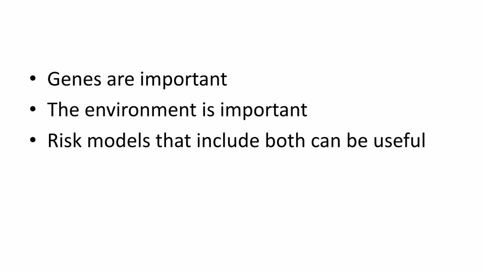
• Genes are important• The environment is important• Risk models that include both can be useful
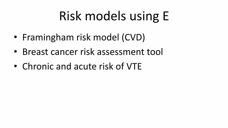
Risk models using E• Framingham risk model (CVD)• Breast cancer risk assessment tool• Chronic and acute risk of VTE
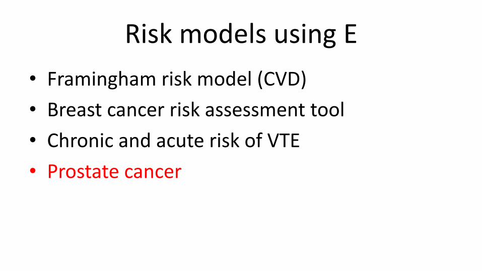
Risk models using E• Framingham risk model (CVD)• Breast cancer risk assessment tool• Chronic and acute risk of VTE• Prostate cancer
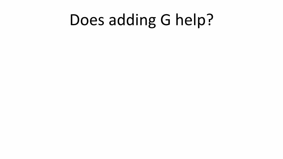
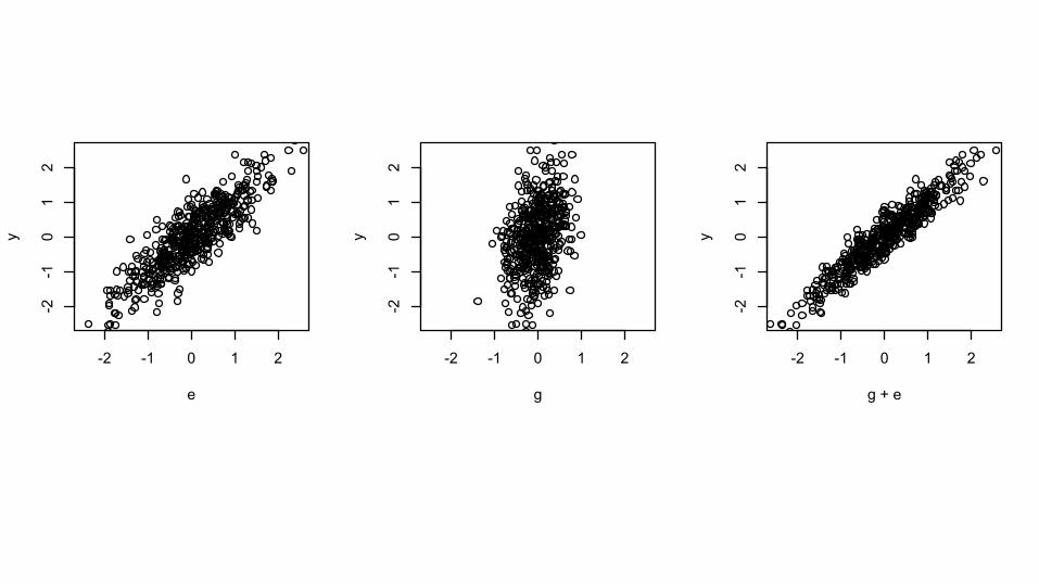
Does adding G help?
-2 -1 0 1 2
-2-1
01
2
e
y
-2 -1 0 1 2
-2-1
01
2g
y-2 -1 0 1 2
-2-1
01
2
g + e
y

-2 -1 0 1 2
-2-1
01
2
e
y
-2 -1 0 1 2
-2-1
01
2g
y-2 -1 0 1 2
-2-1
01
2
g + e
y
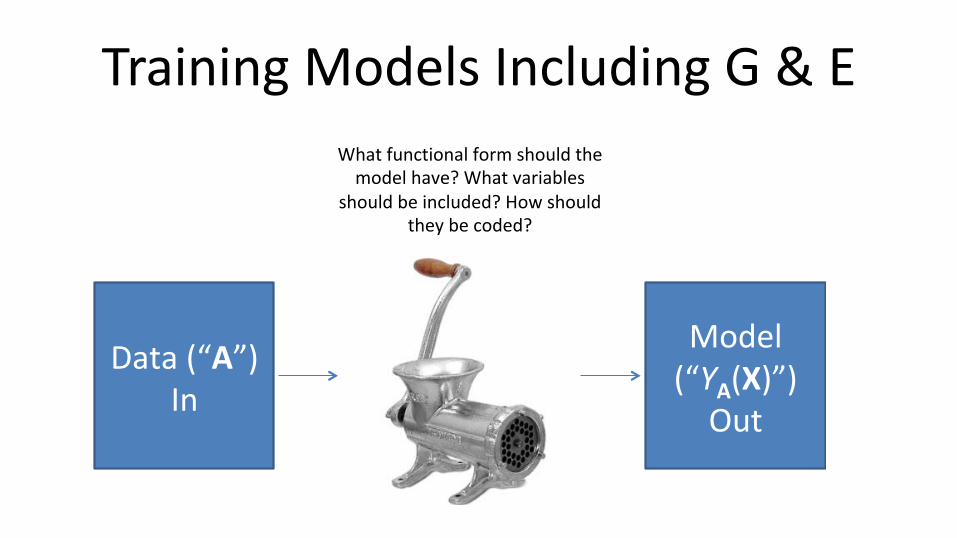
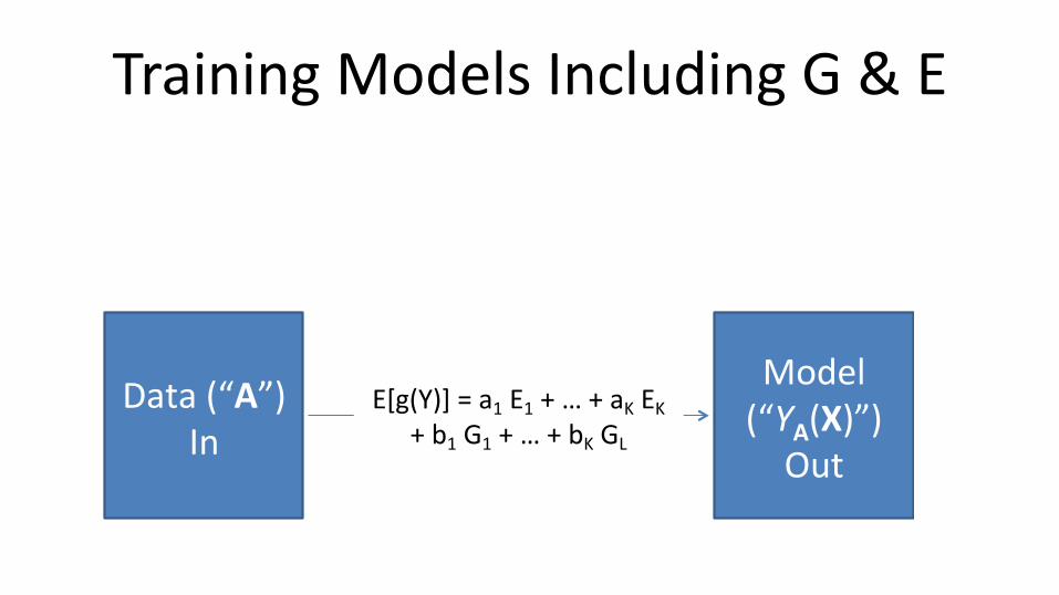
Training Models Including G & E
Data(“A”)In
Model(“YA(X)”)Out
Whatfunctionalformshouldthemodelhave?Whatvariables
shouldbeincluded?Howshouldtheybecoded?
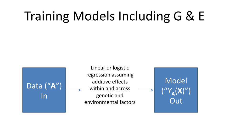
Training Models Including G & E
Data(“A”)In
Model(“YA(X)”)Out
Whatfunctionalformshouldthemodelhave?Whatvariables
shouldbeincluded?Howshouldtheybecoded?
Linear or logistic regression assuming
additive effects within and across
genetic and environmental factors
Data(“A”)In
Model(“YA(X)”)Out
Whatfunctionalformshouldthemodelhave?Whatvariables
shouldbeincluded?Howshouldtheybecoded?
E[g(Y)] = a1 E1 + … + aK EK+ b1 G1 + … + bK GL
Training Models Including G & E
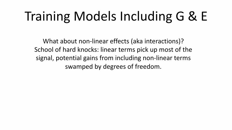
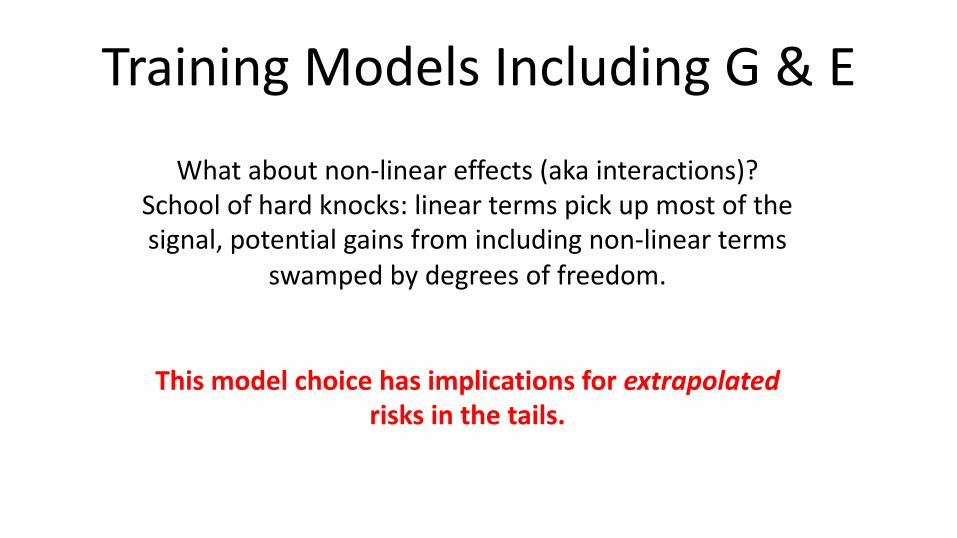
Training Models Including G & EWhat about non-linear effects (aka interactions)?
School of hard knocks: linear terms pick up most of the signal, potential gains from including non-linear terms
swamped by degrees of freedom.
Training Models Including G & EWhat about non-linear effects (aka interactions)?
School of hard knocks: linear terms pick up most of the signal, potential gains from including non-linear terms
swamped by degrees of freedom.
This model choice has implications for extrapolatedrisks in the tails.
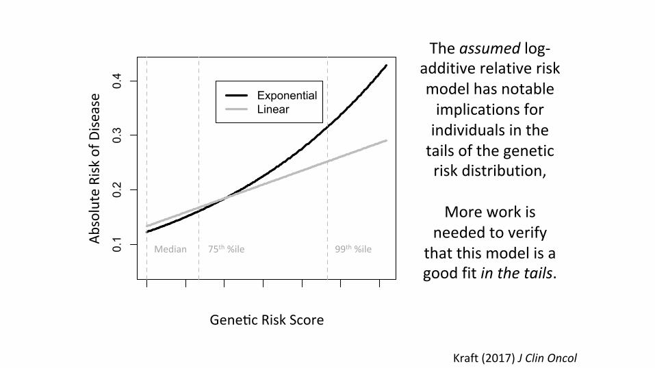
Kraft(2017)JClinOncol
0.0 0.5 1.0 1.5 2.0 2.5 3.0
0.1
0.2
0.3
0.4
g
y3ExponentialLinear
Median 75th%ile 99th%ile
Gene0cRiskScore
AbsoluteRisk
ofD
isease
Theassumedlog-additiverelativeriskmodelhasnotableimplicationsforindividualsinthetailsofthegeneticriskdistribution,
Moreworkis
neededtoverifythatthismodelisagoodfitinthetails.
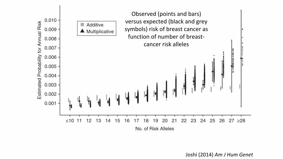
the additive joint-effects model was very strong in magnitudeand highly statistically significant.
Polygenic models used in disease risk prediction have gen-erally assumed multiplicative joint effects of SNPs on the ab-solute risk scale. We find that a multiplicative model for thejoint effects of multiple risk SNPs is substantially better thanan additive model. This provides some support for the use ofa multiplicative model based on individual-SNP marginalodds ratios, as has been suggested in the context of riskscreening and implemented by several consumer geneticscompanies (24, 57–60).
However, the statistically significant submultiplicative de-viation of empirical data from multiplicative effects leavessome scope for improvement. This deviation may reflectthe fact that the external odds ratios used to define the multi-plicative risk score were overestimated due to the “winner’scurse” (61, 62). In sensitivity analyses where we adjusted allper-allele β coefficients by a constant deflation factor (ad-justed β = 0.9 × unadjusted β) or by a factor proportional tothe per-allele odds ratio (ranging from 0.92 to 0.997 (63)),themultiplicativemodelwas amuch betterfit (goodness offit:P = 0.99 for constant adjustment and P = 0.45 for propor-tional adjustment).This suggests thatmultiplicative riskmodelsconstructed using odds ratios from initial discovery publica-tions are likely to be overestimates (or underestimates) in theupper (respectively lower) tails. However, when accurate oddsratio estimates from large studies independent of the originaldiscovery samples are used, a multiplicative polygenic riskmodel may be a good fit, and this model could be utilized toidentify a small number of women at markedly increased riskwho would benefit from risk-reducing interventions or moreintensive screening. We stress that risk estimates for women
in the tails of the risk distribution are projections beyond thesupport of the bulk of the training data and that we had limitedstatistical power to detect departures from multiplicativity inthe tails; note the wide confidence interval for the count ≥28group in Figure 1.
Tests for pairwise interactions between the 23 SNPs failedto show statistically significant departures from additivity be-tween these low-penetrance variants. This may reflect the lowpower to detect small departures from a pairwise additive riskmodel, even with our large sample size. The departure froman additive joint-effects model from the observed fitted risksfor the combination of 19 SNPs suggests the presence of ad-ditive interactions between the SNPs and breast cancer risk.
This study had several other weaknesses. First, althoughdata on exposure variables were prospectively collected inall of the cohorts, the instruments used to collect the informa-tion were not uniform across cohorts, potentially inducing ex-posure misclassification during harmonization. It has beendemonstrated that nondifferential misclassification of 2 inde-pendent exposures preserves the validity of tests for additiveinteraction (64). Furthermore, for ease of interpretation of ad-ditive effects, these exposure variables were represented usingdichotomized categories, which may not be the optimal mod-eling strategy for reflecting their biological associations withbreast cancer. However, in most cases the cutoffs for exposurevariables were not arbitrary, and a priori information was usedto choose them. Similarly, genetic variants were also dichoto-mized assuming a dominant effect for the risk allele, withouta priori evidence for the same.Our results formarginal effects ofmost of the SNPswere not substantially different from results ofprevious studies that assumed log-additive SNP effects. More-over, adjustment for age and cohort may not have sufficiently
0.001
0.002
0.003
0.004
0.005
0.006
0.007
0.008
0.009
0.010
≤10 11 12 13 14 15 16 17 18 19 20 21 22 23 24 25 26 27 ≥28
No. of Risk Alleles
Est
imat
ed P
roba
bilit
y fo
r A
nnua
l Ris
k
AdditiveMultiplicative
Figure 1. Estimated absolute risk of breast cancer according to number of risk alleles among 50-year-old non-Hispanic white females, derivedusing case-control data from the Breast and Prostate Cancer Cohort Consortium (19, 39) and population incidence rates from the Surveillance,Epidemiology, and End Results Program (52), and comparison with expected risk assuming multiplicative and additive joint-effects models.Bars, 95% confidence intervals.
Additive Interactions in Breast Cancer Risk 7
at Harvard Library on O
ctober 10, 2014http://aje.oxfordjournals.org/
Dow
nloaded from
Joshi(2014)AmJHumGenet
Observed(pointsandbars)versusexpected(blackandgreysymbols)riskofbreastcancerasfunctionofnumberofbreast-
cancerriskalleles
Biostatistics (2015), 16, 1, pp. 143–154doi:10.1093/biostatistics/kxu034Advance Access publication on July 14, 2014
Testing calibration of risk models at extremesof disease risk
MINSUN SONGDivision of Cancer Epidemiology and Genetics, National Cancer Institute,
National Institutes of Health, Rockville, MD 20850, USA
PETER KRAFT, AMIT D. JOSHIDepartment of Epidemiology, Harvard School of Public Health, Boston, MA 02115, USA
MYRTO BARRDAHLDivision of Cancer Epidemiology, German Cancer Research Center (DKFZ),
69120 Heidelberg, Germany
NILANJAN CHATTERJEE∗
Division of Cancer Epidemiology and Genetics, National Cancer Institute,National Institutes of Health, Rockville, MD 20850, USA
SUMMARYRisk-prediction models need careful calibration to ensure they produce unbiased estimates of risk forsubjects in the underlying population given their risk-factor profiles. As subjects with extreme high orlow risk may be the most affected by knowledge of their risk estimates, checking the adequacy of riskmodels at the extremes of risk is very important for clinical applications. We propose a new approach to testmodel calibration targeted toward extremes of disease risk distribution where standard goodness-of-fit testsmay lack power due to sparseness of data. We construct a test statistic based on model residuals summedover only those individuals who pass high and/or low risk thresholds and then maximize the test statisticover different risk thresholds. We derive an asymptotic distribution for the max-test statistic based onanalytic derivation of the variance–covariance function of the underlying Gaussian process. The method isapplied to a large case–control study of breast cancer to examine joint effects of common single nucleotidepolymorphisms (SNPs) discovered through recent genome-wide association studies. The analysis clearlyindicates a non-additive effect of the SNPs on the scale of absolute risk, but an excellent fit for the linear-logistic model even at the extremes of risks.
Keywords: Case–control studies; Gene–gene and gene–environment interactions; Genome-wide association studies;Goodness-of-fit tests; Polygenic score; Risk stratification.
∗To whom correspondence should be addressed.
Published by Oxford University Press 2014. This work is written by (a) US Government employee(s) and is in the public domain in the US.
Dow
nloaded from https://academ
ic.oup.com/biostatistics/article-abstract/16/1/143/259068 by H
arvard Library user on 07 May 2019
Biostatistics (2015)
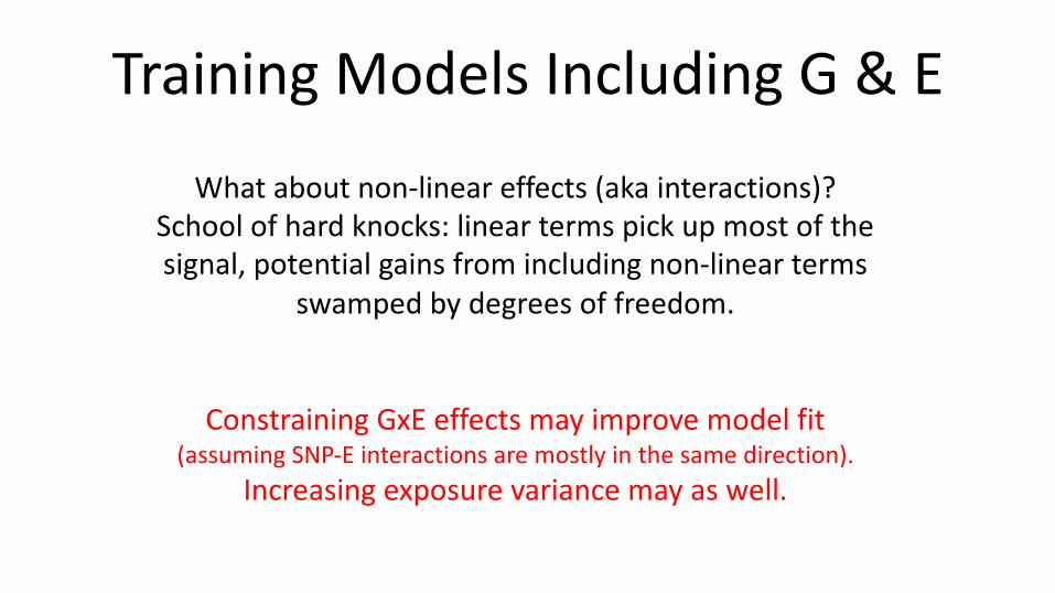
Training Models Including G & EWhat about non-linear effects (aka interactions)?
School of hard knocks: linear terms pick up most of the signal, potential gains from including non-linear terms
swamped by degrees of freedom.
Constraining GxE effects may improve model fit (assuming SNP-E interactions are mostly in the same direction).
Increasing exposure variance may as well.
activity (from sedentary city dwellers to very active rural
farmworkers) identified a qualitatively similar interaction(the minor allele was associated with increased waist size
in the least active subjects but not in the most active;
p = 0.008) in a much smaller sample size (1129) [5].Recent advances in our understanding of common ge-
netic markers associated with a broad range of human traits
and diseases enable us to turn this idea around: we might beable to increase power detect gene–environment interac-
tions by increasing the range genetic susceptibility under
study [6]. Figure 2 contrasts an analysis that focuses on asingle nucleotide polymorphism (SNP) with an analysis
that considers a genetic risk score, for example a multi-
SNP genetic instrument for body mass index, as might beused in a Mendelian randomization study [7]. In this si-
tuation, by capturing more of the relevant genetic vari-
ability, the SNP score increases power to detect gene–environment interaction. This power increase is contingent
on the true joint gene–environment effects having the form
displayed in Fig. 2, or at least on most SNPs in the scorehaving gene–environment interaction effects in the same
direction, but there is already some evidence supporting
interaction effects of this type [8–11].The discussion of exposure misclassification in Stenzel
et al. raises philosophical and increasingly important
practical issues. On a philosophical level, the exposures we
can measure are rarely if ever the etiologically relevantexposures. Some degree of model misspecification and
exposure misclassification is inevitable. But on a practical
level, many of the exposures we can measure and on whichwe could intervene are too expensive to measure directly in
extremely large sample sizes. Instead, epidemiologic
studies rely on inexpensive proxies—a practice which isonly likely to increase, as epidemiologists incorporate
different streams of Big Data into their studies [12]. The
results of Stenzel et al. suggest that the utility of designsthat sample from a larger cohort based on an exposure
proxy in order to identify who to genotype depends on the
accuracy of the proxy. We suspect that the same cautionapplies to designs where the proxy is used to identify a
subset of subjects whose exposures will be measured usinga more expensive ‘‘gold standard’’ technology.
To return to the questions raised above: the relative lack
of compelling gene–environment interactions in humanobservational studies is likely due to both the types of traits
studied and how they are studied. Complex diseases result
from the interplay of multiple biological processes affectedby multiple genes and exposures. Even if an underlying
intermediate trait exhibits strong gene–environment inter-
action, this interaction effect can be washed out at thedisease level. At the same time, limited variability in ex-
posure has likely also contributed to lack of power in hu-
man gene-environment interaction studies. Stenzel et al.demonstrate that thoughtful design can overcome this
limitation. Design and analysis strategies that increase
variability in sampled exposures and genetic suscepti-bilities deserve further consideration.
References
1. Hutter CM, Mechanic LE, Chatterjee N, Kraft P, Gillanders EM.Gene–environment interactions in cancer epidemiology: a Na-tional Cancer Institute Think Tank report. Genet Epidemiol.2013;37(7):643–57. doi:10.1002/gepi.21756.
(a) (b)
nalS
cale
)
me)
Study A
Study B
Study A
Study B
me
(Orig
in
og(O
utco
m
Carrier
Outc
om Lo
Non-carrier
ExposureExposure
Fig. 1 Mean outcome (a) andlog mean outcome (b) as afunction of exposure andgenotype. Arrows denote rangeof exposure captured by twohypothetical studies
GeneticRisk Score
SingleSNP
Exposed
Unexposed
SNPOutc
ome
Genetic Risk
Fig. 2 Mean outcome as a function of exposure and cumulativegenetic risk. Dashed lines denote scaled densities for genetic riskcaptured by a single SNP or a multi-SNP genetic risk score
354 P. Kraft, H. Aschard
123
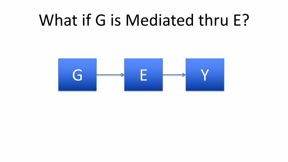
What if G is Mediated thru E?
G E Y
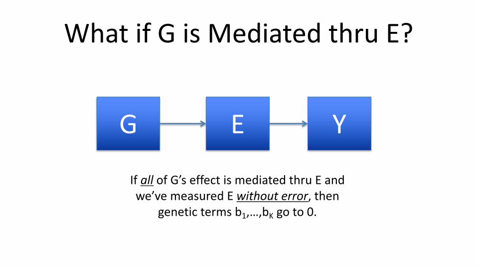
What if G is Mediated thru E?
G E Y
If all of G’s effect is mediated thru E and we’ve measured E without error, then
genetic terms b1,…,bK go to 0.
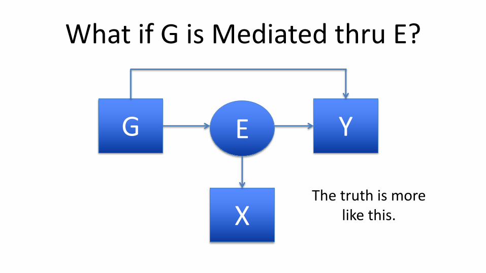
What if G is Mediated thru E?
G YE
XThe truth is more
like this.
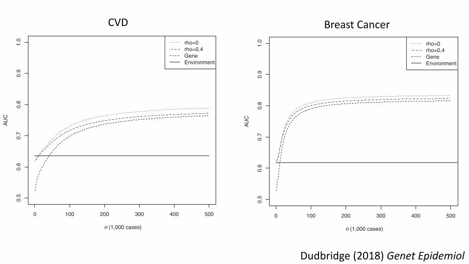
DUDBRIDGE ET AL. 11
T A B L E 2 AUC for environmental score, polygenic score, and combined scores based on a genetic model matching results for CVD reported byMorris et al
Environment Polygenic Unweighted Sum Weighted SumN cases ! = 0.1 ! = 0.4 ! = 0.1 ! = 0.463,746 0.635 0.536 (5× 10⁻⁸) 0.622 (5× 10⁻⁸) 0.621 (5 × 10⁻⁸) 0.623 (5 × 10⁻⁸) 0.622 (5 × 10⁻⁸)63,746 0.635 0.666 (0.053) 0.693 (0.033) 0.688 (0.036) 0.701 (0.053) 0.693 (0.053)∞ 0.635 0.782 0.800 0.784 0.800 0.788
In parentheses, P-value thresholds to select SNPs into polygenic score; N cases, number of cases in training sample with 2.05 controls per case as in CARDIoGRAM-plusC4D.
T A B L E 3 NRI for a single risk threshold of 10% for combined scores based on a genetic model matching results for CVD reported by Morriset al
Unweighted Sum Weighted SumN cases ! = 0.1 ! = 0.4 ! = 0.1 ! = 0.4
Case Control Case Control Case Control Case Control63,746 − 0.0049 0.012 − 0.0038 0.0095 − 0.0060 0.015 0.0053 0.01363,784 − 0.046 (0.79) 0.186 (0.031) − 0.045 (0.76) 0.176 (0.031) − 0.052 (0.85) 0.2 (0.056) − 0.049 (0.86) 0.186 (0.059)∞ − 0.046 0.367 − 0.050 0.344 − 0.046 0.368 − 0.049 0.349
In parentheses, P-value thresholds to select SNPs into polygenic score; N cases, number of cases in training sample with 2.05 controls per case as in CARDIoGRAM-plusC4D.
0 100 200 300 400 500
0.5
0.6
0.7
0.8
0.9
1.0
n (1,000 cases)
AU
C
rho=0rho=0.4GeneEnvironment
F I G U R E 2 AUC of unweighted combined score as a function oftraining sample sizeNote: Genetic model chosen to match results for CVD reported by Mor-ris et al., with 2.05 controls per case as in the CARDIoGRAMplusC4Dconsortium. Rho: chip correlation between environment and outcome.Gene: polygenic score alone. Environment: environmental score alone.
for alternative values of the prevalence and proportion of nullSNPs.
Note that at finite sample size, the optimal P-value thresh-old varies according to the risk threshold and whether the caseor control NRI is maximized, and those thresholds are not theones that maximize AUC. Although the values of NRI are notgreatly changed by using the threshold that maximizes AUC,this shows that the optimal genetic predictor can depend on the
0 100 200 300 400 500
0.5
0.6
0.7
0.8
0.9
1.0
n (1,000 cases)
AU
C
rho=0rho=0.4GeneEnvironment
F I G U R E 3 AUC of weighted combined score as a function oftraining sample sizeNote: Genetic model chosen to match results for CVD reported by Mor-ris et al, with 2.05 controls per case as in the CARDIoGRAMplusC4Dconsortium. Rho: chip correlation between environment and outcome.Gene: polygenic score alone. Environment: environmental score alone.
chosen measure of accuracy. However, the optimal thresholdis the same for continuous NRI and IDI as it is for AUC.
For this model, the optimal threshold to select SNPs atthe CARDIoGRAMplusC4D sample size is at approximatelynominal significance. Although this is well short of genome-wide significance, it results in fewer than 5,000 expected type-1 errors from 100,000 tests and an expected false discoveryrate of about 0.4. It is this false discovery rate, rather than
DUDBRIDGE ET AL. 13
T A B L E 6 NRI for a single-risk threshold of 8%, continuous NRI and IDI for combined scores based on a genetic model matching results forbreast cancer reported by Mavaddat et al
8% Risk Continuous NRI IDIN cases Case Control Case Control33,673 (5 × 10⁻⁸) 0.119 − 0.046 0.286 0.015 0.00833,673 0.303 (0.0034) − 0.059 (0.89) 0.544 (0.0035) 0.029 (0.0035) 0.034 (0.0035)∞ 0.441 − 0.094 0.771 0.041 0.089
In parentheses, P-value thresholds to select SNPs into polygenic score; N cases, number of cases in training sample with 0.99 controls per case as in the Breast CancerAssociation Consortium. ! = 0.4, "2
#$ = 0.8.
0 100 200 300 400 500
0.5
0.6
0.7
0.8
0.9
1.0
n (1,000 cases)
AU
C
rho=0rho=0.4GeneEnvironment
F I G U R E 4 AUC of weighted combined score as a function oftraining sample sizeNote: Genetic model chosen to match results for breast cancer reportedby Mavaddat et al., with 0.99 controls per case as in the Breast CancerAssociation Consortium and "2
#$ = 0.1. Rho: chip correlation betweenenvironment and outcome. Gene: polygenic score alone. Environment:environmental score alone.
not far from the large sample limit. Again, in the near futurethese projections will be refined by further prediction studies.
Table 6 shows NRI at a single risk threshold of 8%, whichis the 10-year absolute risk between ages 40–50 above whichchemoprevention is advised in the United Kingdom (NationalInstitute for Health and Care Excellence, 2013). Again theoptimal SNP selection depends on the criterion optimized.Addition of SNPs to the Gail model would result in case NRIof 0.119 and control NRI of −0.046 when selecting SNPsby % < 5 × 10⁻⁸, improving to case NRI of 0.303 and con-trol NRI of −0.059 with more liberal selection. The negativecontrol NRI implies that more women would be unnecessar-ily recommended to receive chemoprevention, and becausemost women do not develop breast cancer, this translates toa large absolute number of women. Indeed the specificity forthe development of cancer is 92% for the environmental scorealone, but is 86% for the combined score, whereas the sensi-tivities are 16% and 32% respectively. Thus, while AUC and
NRI appear encouraging, a large number of women would infact be misclassified under either score. The continuous NRIshows that over half of cases are expected to increase theirrisk score. Supplementary Tables S9 and S10 show resultsfor alternative values of the prevalence and proportion of nullSNPs.
Reflecting applications in screening, the breast cancer liter-ature emphasises the proportion of cases present within somehighest-risk proportion of the population (Pharoah, Anto-niou, Easton, & Ponder, 2008). This is a point on a Lorenzcurve, which resembles the receiver-operator characteristiccurve with specificity replaced by a population proportion.For a proportion of the population q at highest risk accord-ing to score X, the corresponding threshold of liability is√
&2$Φ−1(1 − ') and so the proportion of cases selected by
that threshold is:
1 − Φ⎛⎜⎜⎜⎝
√&2$Φ
−1(1 − ') − (($|) = 1)√var($|) = 1)
⎞⎟⎟⎟⎠.
Table 7 shows the proportion of cases within the top 10%,20%, and 50% of the population at highest risk according tothe environmental score X and the combined score +̂,-./.These results suggest, for example, that at current samplesizes nearly half of cases could be detected by screening the20% of the population with highest combined scores. Withlarger training samples, over 90% of cases might be detectedby screening the half of the population with highest scores.These results are compatible with those of previous studies(Garcia-Closas et al., 2014; Pharoah et al., 2008). Supple-mentary Tables S11 and S12 show results for alternative val-ues of the prevalence and proportion of null SNPs. Similar toother sensitivity analyses in the supplementary tables, theseyield modest quantitative changes with similar qualitativeconclusions.
3.3 HeightHere the example of height is used to illustrate a relation-ship between a polygenic score and family history. Of course,family history is an environmental risk factor for any heri-
CVD Breast Cancer
Dudbridge (2018) Genet Epidemiol
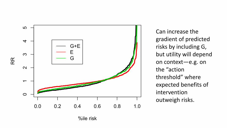
So, is it useful?• Spreading risk distribution• Identifying subgroups where G is actionable
0.0 0.2 0.4 0.6 0.8 1.0
01
23
45
%ile risk
RR
G+EEG
Can increase the gradient of predicted risks by including G, but utility will depend on context—e.g. on the “action threshold” where expected benefits of intervention outweigh risks.
0.0 0.2 0.4 0.6 0.8 1.0
01
23
45
%ile risk
RR
G+EEG
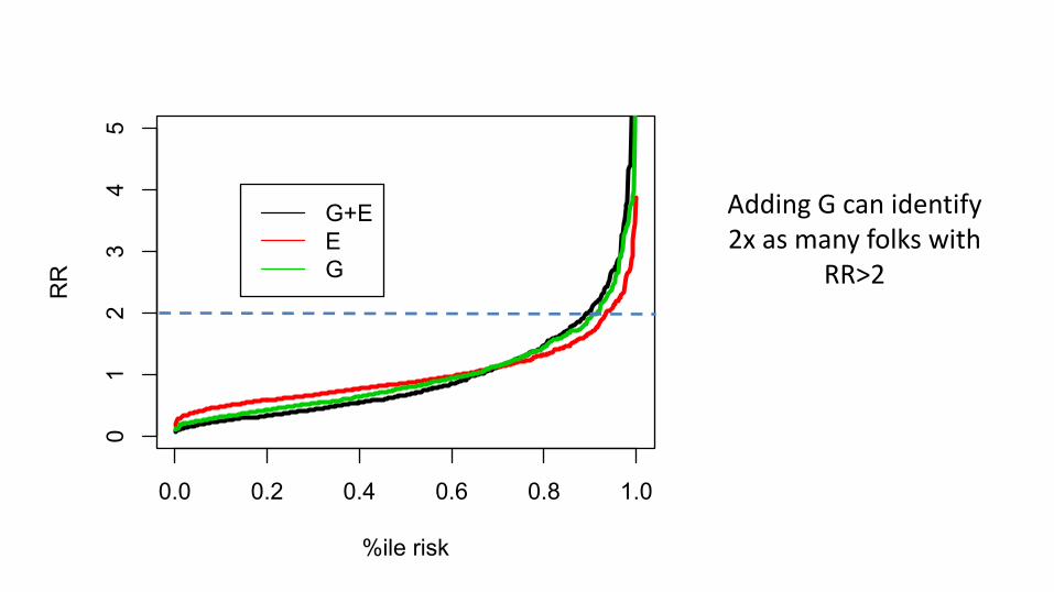
Adding G can identify 2x as many folks with
RR>2
0.0 0.2 0.4 0.6 0.8 1.0
01
23
45
%ile risk
RR
G+EEG
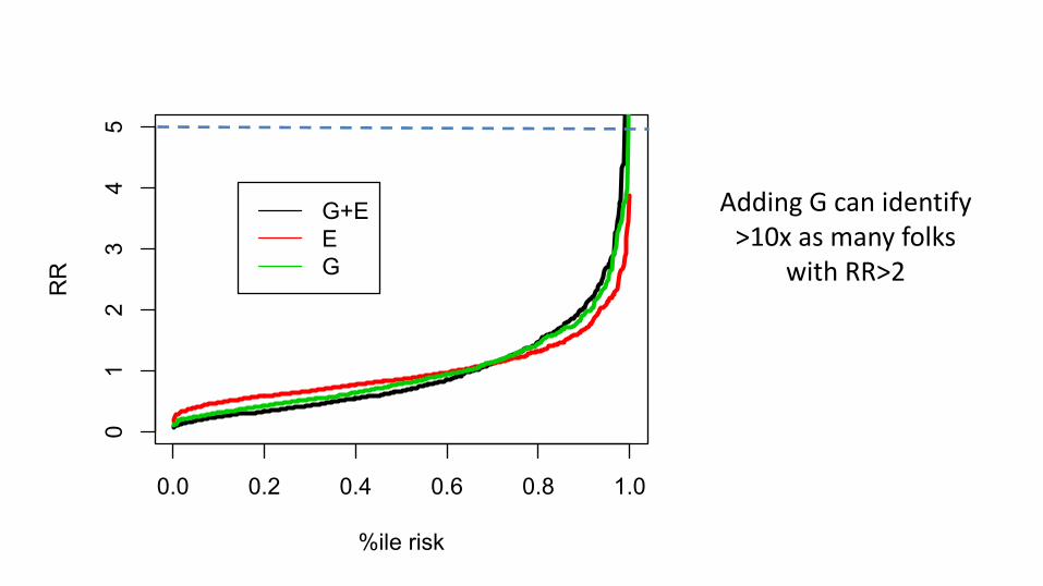
Adding G can identify >10x as many folks
with RR>2
The PAR is commonly used to approximate the publichealth implications of modifying or removing an exposure.Although it is a useful quantifiable estimate of the impact of acausal factor (in this case, genetic risk), it can rapidlyapproach the upper bound of 100%, if the risk allelefrequency and relative risk of the disease are high, and maybe more inflated than other measures of genetic risk, such asthe heritability of disease liability, approximate heritability,sibling recurrence risk, and overall genetic variance using alog relative risk scale (Witte et al., 2014). The PAR is based onthe excess fraction of disease that is associated with thepresence of these risk alleles, but not necessarily the etiologicfraction, or the fraction of disease that truly arises due to theserisk alleles. An additional limitation of the multi-locus PARand the polygenic risk score based on these loci is that theydo not account for interactions among SNPs. Furthermore, itshould be noted that these GWAS were done primarily innon-Hispanic white populations so these risks may nottranslate to other ethnic groups.
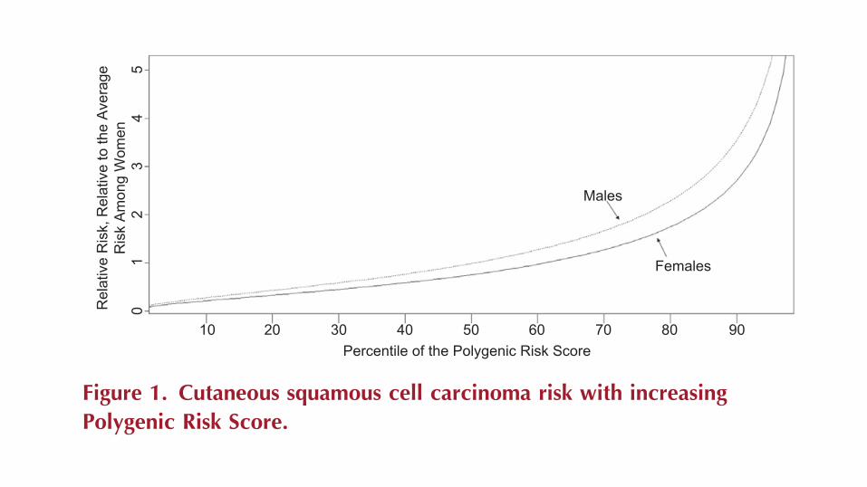
Despite these limitations, the multi-locus populationattributable risk and its related polygenic risk score arepromising tools for identifying those individuals at greatestrisk for cSCC, who would benefit from enhanced monitoring,and those individuals who are at lowest cSCC risk, for whomenhanced monitoring would be time-consuming, costly, andunnecessary. Development of such a risk prediction tool forcSCC would benefit from further refinement that includesgeneeenvironment interactions and from validation acrossdifferent populations, but would have the potential to beclinically meaningful, impacting both screening andprevention efforts. Next-generation studies relating thepolygenic contribution to cSCC risk will likely incorporatenewly discovered rare variants. Future studies may alsoinclude variants identified through meta-analyses of existingas well as forthcoming cSCC GWAS, which will increaseboth the power and robustness of genetic associations used toderive the polygenic risk score.
MATERIALS AND METHODSWe performed a search of the published literature using standard
search strategies involving the querying of two online databases
(MEDLINE and Cochrane) using key words squamous cell carci-
noma, skin, and genome-wide association from January 1980 to
January 31, 2017, followed by evaluation of the bibliographies of
relevant articles, and identified three GWAS that utilized cohorts
from Kaiser Permanente Northern California, Nurses’ Health Study,
the Health Professionals Follow-up Study, the Rotterdam Study,
and the 23andMe (Asgari et al., 2016; Chahal et al., 2016;
Siiskonen et al., 2016). We excluded one study that was primar-
ily a basal cell carcinoma GWAS that tested significant basal cell
carcinoma!associated SNP variants for their relationship with
cSCC, and was not a true SCC GWAS (Nan et al., 2011). Whereas
our methodology was not a formalized systematic review, we did
capture all published cSCC GWAS data. We compiled all SNPs
associated with cSCC that replicated in independent populations.
Odds ratios for SNPs associated with cSCC were used for the multi-
locus PAR calculations, and all studies assumed an additive
genetic model. We focused on bi-allelic SNPs, removing one
tri-allelic SNP, duplicates, or SNPs in linkage disequilibrium. If the
same SNP was reported in more than one GWAS, or if two SNPs at
the same locus were in linkage disequilibrium (R2 > 0.3), we used
the odds ratio from the largest study for the multi-locus PAR and
polygenic risk score calculations. Odds ratios for individual risk
alleles, as well as the multi-locus PAR for all alleles combined, are
shown in Table 1. The multi-locus PAR is weighted most heavily by
the risk alleles with both the highest prevalence and largest odds
ratios for cSCC. We used the formula below (derived from Rockhill
et al., 1998) to compute the multi-locus PAR
1! 1
1þPi
!SjpijRRij
"
where i indexes SNP, and j indexes genotype at each SNP.
We also estimated the population distribution of polygenic risk
scores based on published cSCC GWAS. For risk prediction based on
multiple loci, we assumed a log-additive model for the joint effects
of SNPs and constructed polygenic risk scores by summing the
number of alleles across SNPs:
logðrelative riskÞ ¼ aþ SibiGi
Here bi is the log odds ratio per risk allele at SNP i (given in Table 1)
and Gi is the count of risk alleles at locus i and a is chosen so that the
average relative risk is 1.
The standard deviation of the polygenic risk score was calculated
as follows,
ffiffiffiffiffiffiffiffiffiffiffiffiffiffiffiffiffiffiffiffiffiffiffiffiffiffiffiffiffiffiffiffiffiSi2qi
$1! qi
%b2i
q
where bi is log relative risk w log odds ratio for SNPi and qi is
(1 e risk allele frequency). For SNPs that were reported as protective,
we used the major allele as the risk allele in our calculations, along
with the corresponding cSCC odds ratio for the major allele. The
standard deviation of the polygenic risk score can be used to plot the
distribution of the relative risk due to known common SNPs: Relative
risk of cSCC per polygenic risk score percentile is shown in Figure 1,
with lines plotted for both males and females. We have plotted
percentiles of the polygenic risk score in relation to cSCC risk, rather
than the raw values themselves, to facilitate interpretation of the
score relative to the population. The plot for males accounts for
the underling increased risk of cSCC in male subjects (relative
risk ¼ 1.31 for males vs. females) (Whiteman et al., 2016).
CONFLICT OF INTERESTThe authors state no conflicts of interest.
10 20 30 40 50Percentile of the Polygenic Risk Score
Rel
ativ
e R
isk,
Rel
ativ
e to
the
Aver
age
Ris
k Am
ong
Wom
en5
43
21
0
60 70
Males
Females
80 90
Figure 1. Cutaneous squamous cell carcinoma risk with increasingPolygenic Risk Score.
JE Sordillo et al.cSCC Attributable Risk
www.jidonline.org 1509
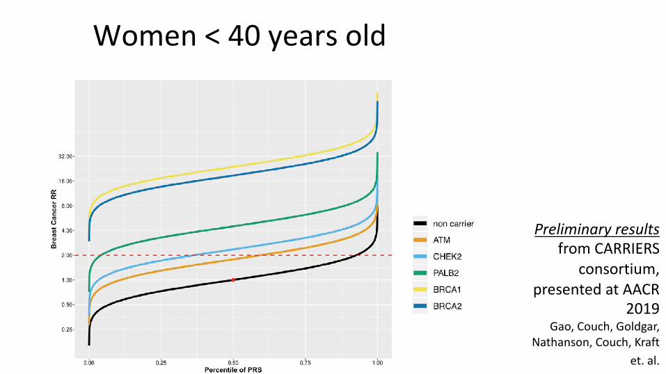
Women<40yearsold
Preliminary resultsfrom CARRIERS
consortium, presented at AACR
2019Gao, Couch, Goldgar,
Nathanson, Couch, Kraft et. al.
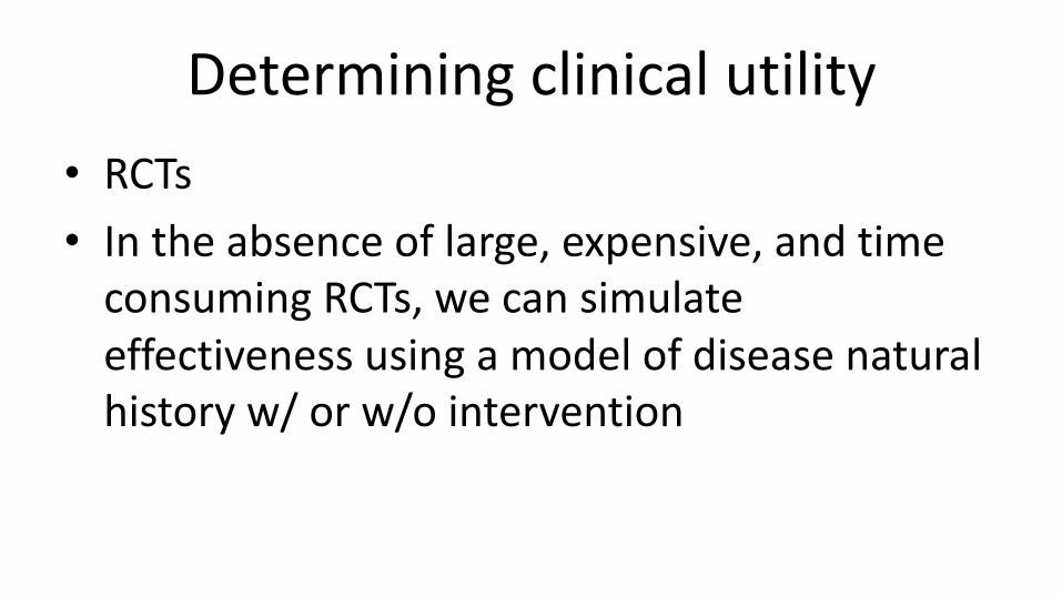
Determining clinical utility• RCTs• In the absence of large, expensive, and time
consuming RCTs, we can simulate effectiveness using a model of disease natural history w/ or w/o intervention
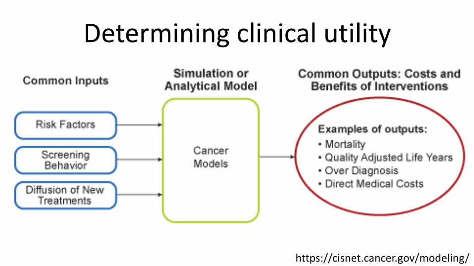
Determining clinical utility
https://cisnet.cancer.gov/modeling/
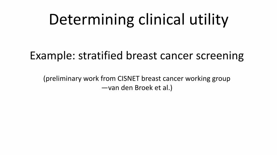
Example: stratified breast cancer screening
(preliminary work from CISNET breast cancer working group—van den Broek et al.)
Determining clinical utility
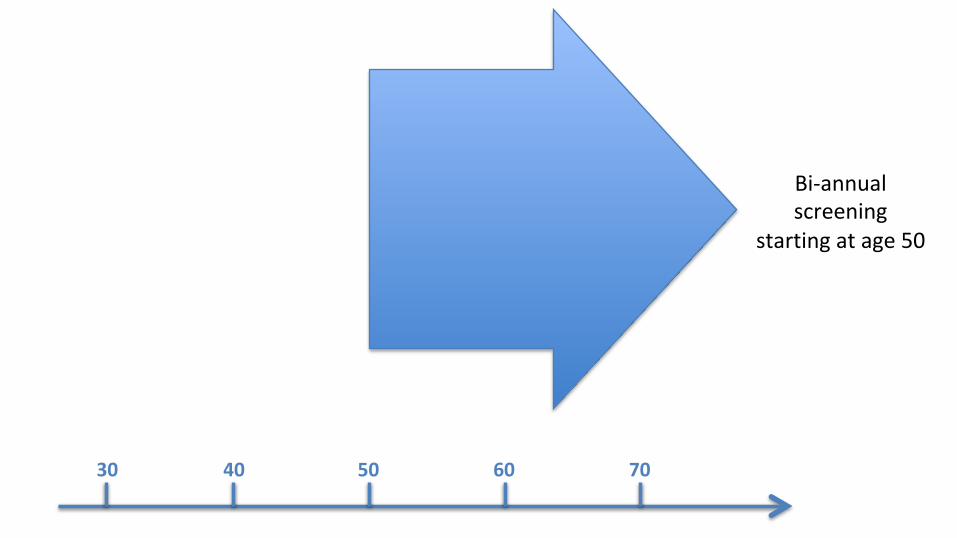
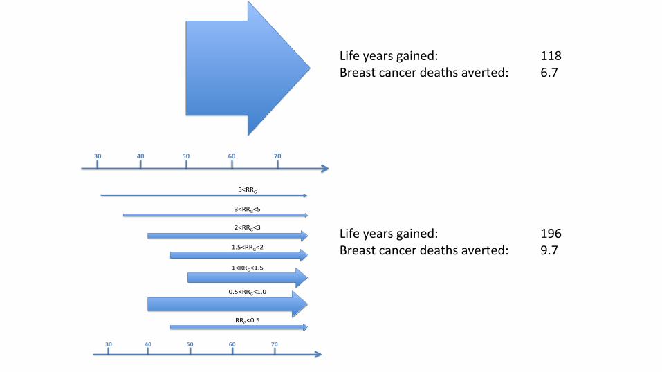
30 40 50 60 70
Bi-annualscreening
startingatage50
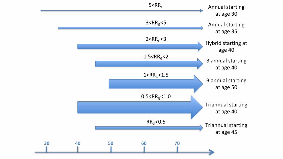
30 40 50 60 70
Annualstartingatage30
Annualstartingatage35
Hybridstartingatage40
Biannualstartingatage40
Biannualstartingatage50
Triannualstartingatage40
Triannualstartingatage45
5<RRG
3<RRG<5
2<RRG<3
1.5<RRG<2
1<RRG<1.5
0.5<RRG<1.0
RRG<0.5
30 40 50 60 70
30 40 50 60 70
5<RRG
3<RRG<5
2<RRG<3
1.5<RRG<2
1<RRG<1.5
0.5<RRG<1.0
RRG<0.5
Lifeyearsgained: 118Breastcancerdeathsaverted: 6.7
Lifeyearsgained: 196Breastcancerdeathsaverted: 9.7
VandenBroek(inprogress)
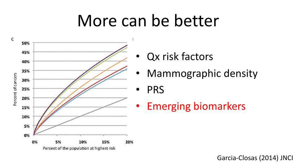
More can be better
• Qx risk factors• Mammographic density• PRS• Emerging biomarkers
Page 4 of 6 Commentary | JNCI
(ie, lifetime risk of 17%-30%). However, the use of these drugs requires identification of women at those levels of risk. Our cal-culations based on all risk factors combined indicate that about 10% of women 50 years old found to be at moderate to high
risk (capturing about 27% of cases in the population) could be identified as eligible for chemoprevention (Model 5 in Table 1), thus benefiting from a 38% reduction in risk (4). This could be improved to 11% of women capturing about 34% of cases when
Figure 1. Partial Receiver Operating Curves (ROC) showing the percent-age of cases of breast cancer expected to occur in groups of the popu-lation at highest predicted risk (A, C), and graphs for the percentage of the population crossing breast cancer relative risk (RR) thresholds (compared with the average risk in the population) (B, D). Estimates are for a UK population of women aged 50 years, for eight risk prediction
models, including different sets of risk factors and two polygenic risk scores (PRSs): the 76–single nucleotide polymorphism (SNP) PRS based on currently known SNPs explaining 15% of the familial risk (A, B) and an improved PRS explaining 30% of the familial risk (C, D). PRS = polygenic risk score; Qx = questionnaire; SNP = single nucleotide polymorphism.
Dow
nlo
aded fro
m h
ttps://a
cadem
ic.o
up.c
om
/jnci/a
rticle
-abstra
ct/1
06/1
1/d
ju305/1
499201 b
y H
arv
ard
Colle
ge L
ibra
ry, C
abot S
cie
nce L
ibra
ry u
ser o
n 0
7 M
ay 2
019
Garcia-Closas (2014) JNCI
Misc Issues• Implementing “complicated” E models
—good locally, maybe not globally• Including biology in risk models


![RESEARCH ARTICLE OpenAccess ......SNP discovery and genotyping array development in pea [12-15]. SNP markers have been widely used in a large range of living organisms both for genetic](https://img.pdfslide.net/doc/110x75/60b9c020070cae73854476ff/research-article-openaccess-snp-discovery-and-genotyping-array-development.jpg)


![Estimation of genetic variation and SNP- heritability … · [Visscheret al. 2010, Twin Research and Human Genetics] 13 Checking for population structure. Genetic variance associated](https://img.pdfslide.net/doc/110x75/5b9512b709d3f2de4a8b8428/estimation-of-genetic-variation-and-snp-heritability-visscheret-al-2010.jpg)