Embed Size (px)
Citation preview
Clifton Callender
College of Music, Florida State University.
Ian Quinn
Music Department, Yale University.
Dmitri Tymoczko
Music Department, Princeton University.
To whom correspondence should be addressed.
All three authors contributed equally to this report.
GENERALIZED VOICE-LEADING SPACES
SUMMARY: We translate basic concepts of music theory into the language of
contemporary geometry.
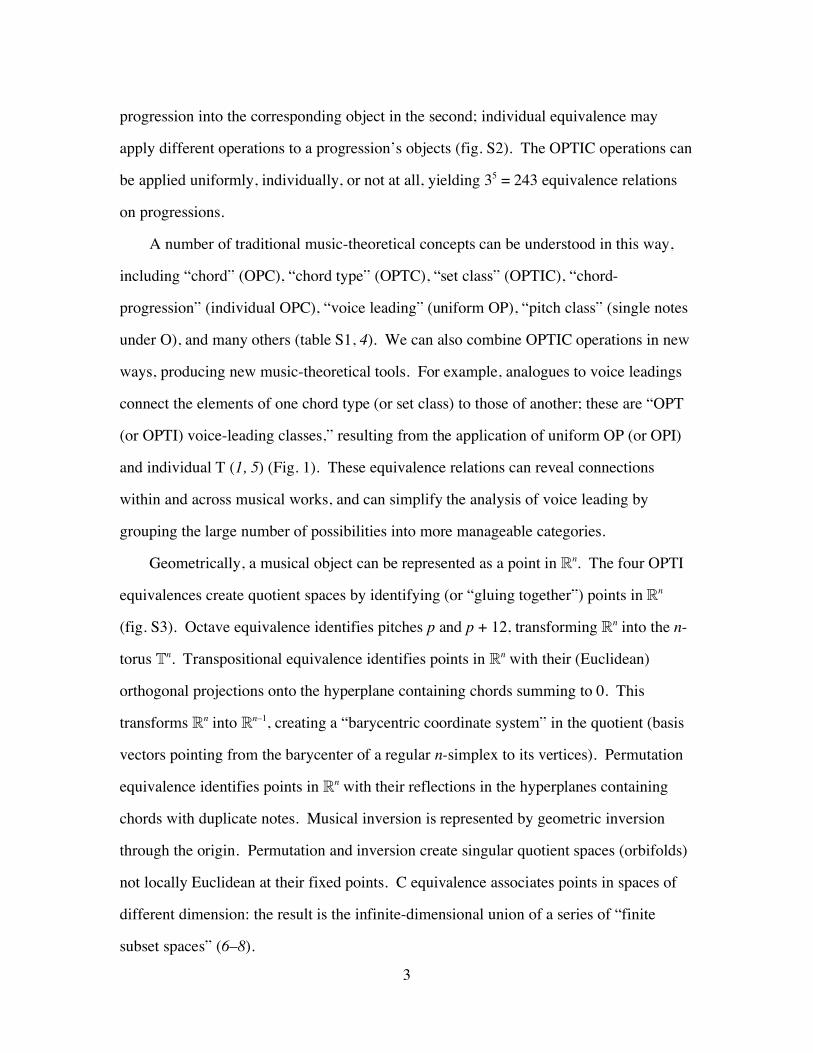
ABSTRACT: Western musicians traditionally classify pitch sequences by disregarding
the effects of five musical transformations: octave shift, permutation, transposition,
inversion, and cardinality change. Here we model this process mathematically, showing
that it produces 32 equivalence relations on chords, 243 equivalence relations on chord
sequences, and 32 families of geometrical quotient spaces, in which both chords and
chord-sequences are represented. This model reveals connections between music-
theoretical concepts, yields new analytical tools, unifies existing geometrical
representations, and suggests a way to understand similarity between chord-types.
2
To interpret music is to ignore information. A capable musician can understand the
sequence of notes (C4, E4, G4) in various ways: as an ordered pitch sequence (an
“ascending C-major arpeggio starting on middle C”), an unordered collection of octave-
free note-types (a “C major chord”), an unordered collection of octave-free note-types
modulo transposition (a “major chord”), and so on. Musicians commonly abstract away
from five types of information: the octave in which notes appear, their order, their
specific pitch level, whether a sequence appears “rightside up” or “upside down”
(inverted), and the number of times a note appears. Different purposes require different
information; consequently, there is no one optimal degree of abstraction.
Here we model this process. We represent pitches using the logarithms of their
fundamental frequencies, setting middle C at 60 and the octave equal to 12. A musical
object is a sequence of pitches ordered in time or by instrument (1): the object (C4, E4,
G4) can represent consecutive pitches played by a single instrument, or a simultaneous
event in which the first instrument plays C4, the second E4 and the third G4. (Instruments
can be ordered arbitrarily.) Musicians generate equivalence classes (2, 3) of objects by
ignoring five kinds of transformation: octave shifts (O), which move any note in an
object into any other octave; permutations (P), which reorder an object; transpositions
(T), which move all the notes in an object in the same direction by the same amount;
inversions (I), which turn an object “upside down”; and cardinality changes (C), which
insert duplications into an object (4) (fig. S1, Table 1). (Note that O operations can move
just one of an object’s notes, while T operations move all notes.) We can form
equivalence relations using any combination of the OPTIC operations, yielding 25 = 32
possibilities.
A musical progression is an ordered sequence of musical objects. Let F be a
collection of musical transformations, with f, f1,…, fn F . The progression (p1, …, pn) is
uniformly F-equivalent to (f(p1), …, f(pn)) and individually F-equivalent to (f1(p1), …,
fn(pn)). Uniform equivalence uses a single operation to transform each object in the first
3
progression into the corresponding object in the second; individual equivalence may
apply different operations to a progression’s objects (fig. S2). The OPTIC operations can
be applied uniformly, individually, or not at all, yielding 35 = 243 equivalence relations
on progressions.
A number of traditional music-theoretical concepts can be understood in this way,
including “chord” (OPC), “chord type” (OPTC), “set class” (OPTIC), “chord-
progression” (individual OPC), “voice leading” (uniform OP), “pitch class” (single notes
under O), and many others (table S1, 4). We can also combine OPTIC operations in new
ways, producing new music-theoretical tools. For example, analogues to voice leadings
connect the elements of one chord type (or set class) to those of another; these are “OPT
(or OPTI) voice-leading classes,” resulting from the application of uniform OP (or OPI)
and individual T (1, 5) (Fig. 1). These equivalence relations can reveal connections
within and across musical works, and can simplify the analysis of voice leading by
grouping the large number of possibilities into more manageable categories.
Geometrically, a musical object can be represented as a point in Rn. The four OPTI
equivalences create quotient spaces by identifying (or “gluing together”) points in Rn
(fig. S3). Octave equivalence identifies pitches p and p + 12, transforming Rn into the n-
torus Tn. Transpositional equivalence identifies points in Rn with their (Euclidean)
orthogonal projections onto the hyperplane containing chords summing to 0. This
transforms Rn into Rn–1, creating a “barycentric coordinate system” in the quotient (basis
vectors pointing from the barycenter of a regular n-simplex to its vertices). Permutation
equivalence identifies points in Rn with their reflections in the hyperplanes containing
chords with duplicate notes. Musical inversion is represented by geometric inversion
through the origin. Permutation and inversion create singular quotient spaces (orbifolds)
not locally Euclidean at their fixed points. C equivalence associates points in spaces of
different dimension: the result is the infinite-dimensional union of a series of “finite
subset spaces” (6–8).
4
One can apply any combination of the OPTI equivalences to Rn, yielding 24 = 16
quotient spaces for each dimension (Table 1); applying C produces 16 additional infinite-
dimensional quotients. Any ordered pair of points in any quotient space represents an
equivalence class of progressions related individually by the relevant combination of
OPTIC equivalences. The image of a line segment in Rn (a “line segment” in the
quotient, though it may “bounce off” a singularity [1, 9]) can be identified with an
equivalence class of progressions related uniformly by the relevant combination of OPIC
and individually by T. (This is because T acts by orthogonal projection.) Intuitively,
pairs of points represent successions between equivalence classes, considered as
indivisible harmonic wholes; line segments represent specific connections between their
elements.
Music theorists have proposed numerous geometrical models of musical structure
(fig. S4, table S3), many of which are regions of the spaces described in this report.
These models have often been incomplete, displaying only a portion of the available
chords or chord-types, and omitting singularities and other non-trivial geometrical and
topological features. Furthermore, they have been explored in isolation, without an
explanation of how they are derived or how they relate (10). Our model resolves these
issues by describing the complete family of continuous n-note spaces corresponding to
the 32 OPTIC equivalence relations.
Of these, the most useful are the OP, OPT, and OPTI spaces, representing voice-
leading relations among chords, chord types, and set classes, respectively (4). The OP
spaces Tn/Sn (n-tori modulo the symmetric group) have been described previously (9).
The OPT space Tn-1/Sn is the quotient of an (n–1)-simplex, whose boundary is singular,
by the rigid transformation cyclically permuting its vertices (4). The OPTI space
Tn-1/(Sn Z2) is the quotient of the resulting space by an additional reflection. These
spaces can be visualized as oblique cones over quotients of the (n–2)-sphere, albeit with
additional orbifold points. The singular point at the cone’s “vertex” contains the chord-
5
type that divides the octave into n equal pieces; the more closely a chord-type’s notes
cluster together, the farther it is from this point. The singular base of conical OPT space
can be visualized as the quotient of the (n–2)-sphere by the cyclic group Zn. (When n is
prime, this is a lens space; when n is not prime, it does not in general seem to have a
familiar name.) The base acts like a mirror, containing chords with note duplications.
The OPTI-spaces Tn-1/(Sn Z2) are essentially similar: they can be visualized as cones
over the quotients of the (n–2)-sphere by the dihedral group Zn Z2, with Z2
representing central inversion.
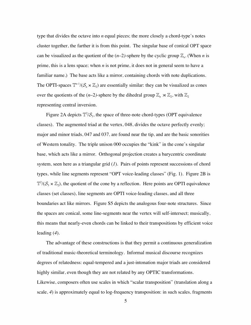
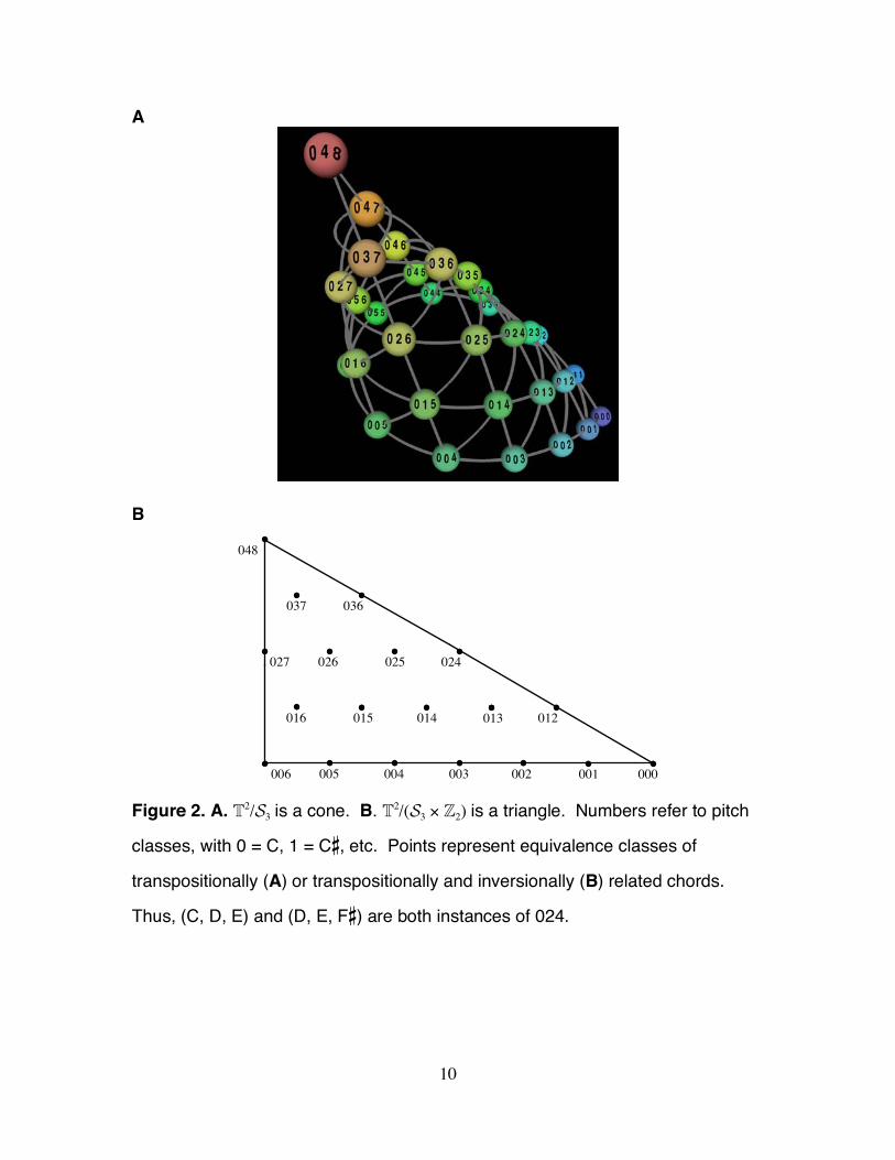
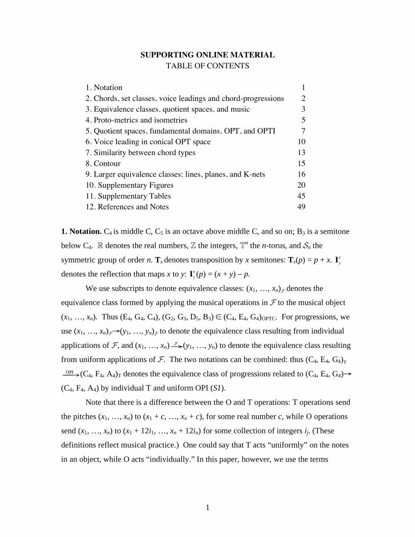
Figure 2A depicts T2/S3, the space of three-note chord-types (OPT equivalence
classes). The augmented triad at the vertex, 048, divides the octave perfectly evenly;
major and minor triads, 047 and 037, are found near the tip, and are the basic sonorities
of Western tonality. The triple unison 000 occupies the “kink” in the cone’s singular
base, which acts like a mirror. Orthogonal projection creates a barycentric coordinate
system, seen here as a triangular grid (1). Pairs of points represent successions of chord
types, while line segments represent “OPT voice-leading classes” (Fig. 1). Figure 2B is
T2/(S3 Z2), the quotient of the cone by a reflection. Here points are OPTI equivalence
classes (set classes), line segments are OPTI voice-leading classes, and all three
boundaries act like mirrors. Figure S5 depicts the analogous four-note structures. Since
the spaces are conical, some line-segments near the vertex will self-intersect; musically,
this means that nearly-even chords can be linked to their transpositions by efficient voice
leading (4).
The advantage of these constructions is that they permit a continuous generalization
of traditional music-theoretical terminology. Informal musical discourse recognizes
degrees of relatedness: equal-tempered and a just-intonation major triads are considered
highly similar, even though they are not related by any OPTIC transformations.
Likewise, composers often use scales in which “scalar transposition” (translation along a
scale, 4) is approximately equal to log-frequency transposition: in such scales, fragments
6
such as C-D-E (“Do, a deer”) and D-E-F (“Re, a drop”) are considered similar, even
though they are not OPTIC-equivalent. Traditional music theory, however, has often
adopted a binary approach to classification: chords are considered equivalent if they can
be related by OPTIC transformations, and are considered unrelated otherwise (2).
Several theorists have recently criticized this view, and modeling similarity between
chord types is an active area of music-theoretical research (4, 11). However, no existing
model describes the broad flexibility inherent in ordinary musical terminology: for
example, none explains the similarity between just and equal-tempered major triads.
Our spaces suggest such a measure. Nearby points represent equivalence classes
whose members can be linked by small voice leadings; in this sense, they are nearly
equivalent modulo the relevant equivalence relation. This model is in good accord with
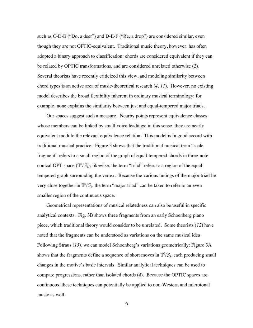
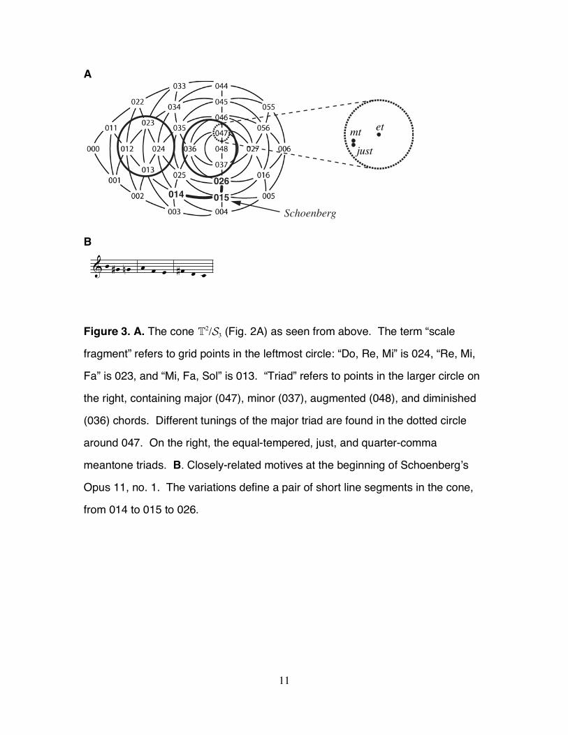
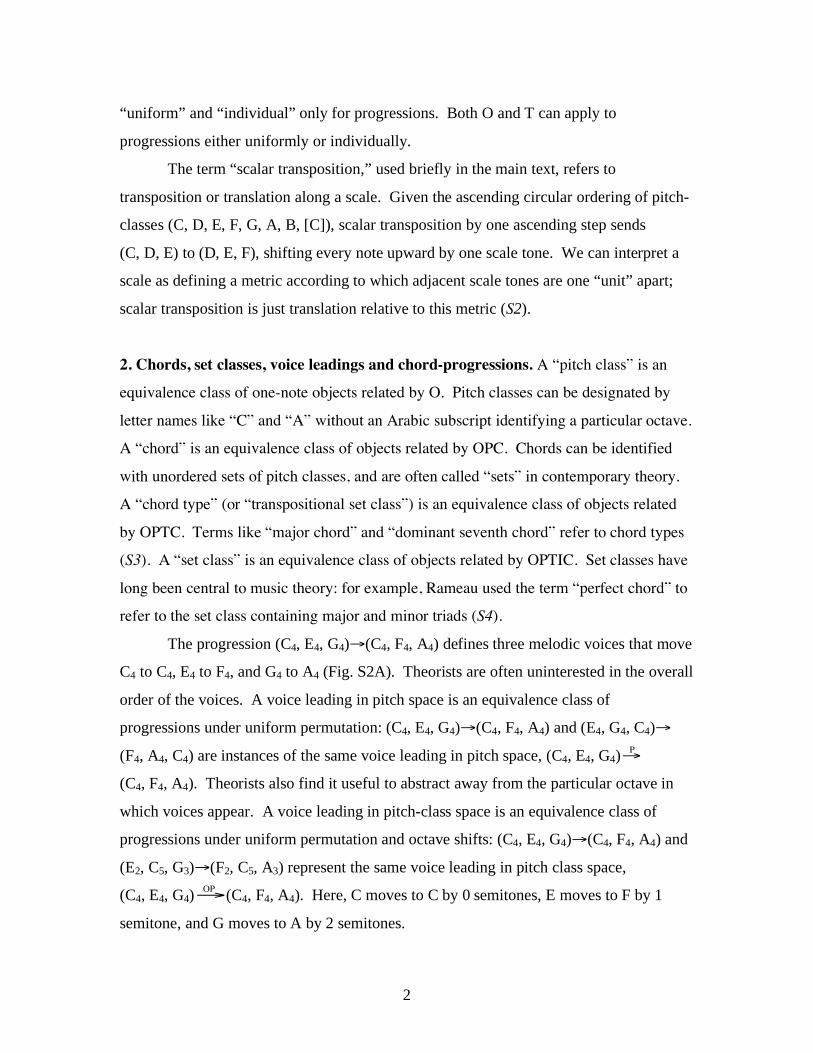
traditional musical practice. Figure 3 shows that the traditional musical term “scale
fragment” refers to a small region of the graph of equal-tempered chords in three-note
conical OPT space (T2/S3); likewise, the term “triad” refers to a region of the equal-
tempered graph surrounding the vertex. Because the various tunings of the major triad lie
very close together in T2/S3, the term “major triad” can be taken to refer to an even
smaller region of the continuous space.
Geometrical representations of musical relatedness can also be useful in specific
analytical contexts. Fig. 3B shows three fragments from an early Schoenberg piano
piece, which traditional theory would consider to be unrelated. Some theorists (12) have
noted that the fragments can be understood as variations on the same musical idea.
Following Straus (13), we can model Schoenberg’s variations geometrically: Figure 3A
shows that the fragments define a sequence of short moves in T2/S3, each producing small
changes in the motive’s basic intervals. Similar analytical techniques can be used to
compare progressions, rather than isolated chords (4). Because the OPTIC spaces are
continuous, these techniques can potentially be applied to non-Western and microtonal
music as well.
7
Beyond modeling musical similarity, the geometrical perspective provides a unified
framework for investigating a wide range of contemporary music-theoretical topics,
including “contour” and “K-nets” (4, 14, 15). This is not surprising, as the OPTIC
equivalences have been central to Western musical discourse since at least the
seventeenth century (16). Our model translates these music-theoretical terms into precise
geometrical language, revealing a rich set of mathematical consequences. This
translation may have implications for theory, analysis, pedagogy, composition, musical
data analysis and visualization, and perhaps even the design of new musical instruments.
8
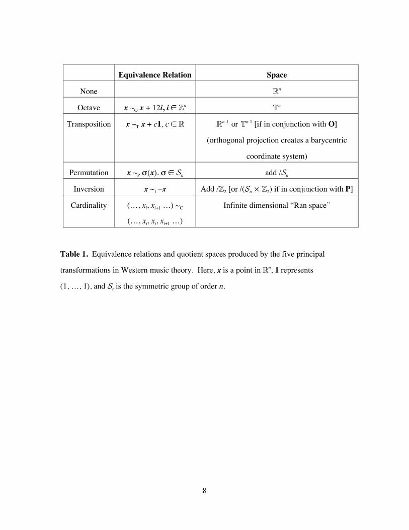
Equivalence Relation Space
None Rn
Octave x ~O x + 12i, i Zn Tn
Transposition x ~T x + c1, c R Rn-1
or Tn-1 [if in conjunction with O]
(orthogonal projection creates a barycentric
coordinate system)
Permutation x ~P (x), Sn add /Sn
Inversion x ~I –x Add /Z2 [or /(Sn Z2) if in conjunction with P]
Cardinality (…, xi, xi+1 …) ~C
(…, xi, xi, xi+1 …)
Infinite dimensional “Ran space”
Table 1. Equivalence relations and quotient spaces produced by the five principal
transformations in Western music theory. Here, x is a point in Rn, 1 represents
(1, …, 1), and Sn is the symmetric group of order n.
9
A B C D E F
&
?
œ œ
œ œ
œb œ
œ# œ
œ# œ
œ# œ
œ œ
œb œ
œ œ&
œ œ#œ œ
œ# œnœ œ
œ œœ œb
œ# œb
œ œ
œ œœb œ#
œb œnœ œ
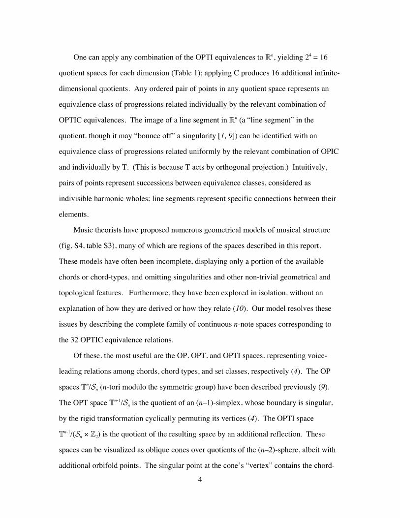
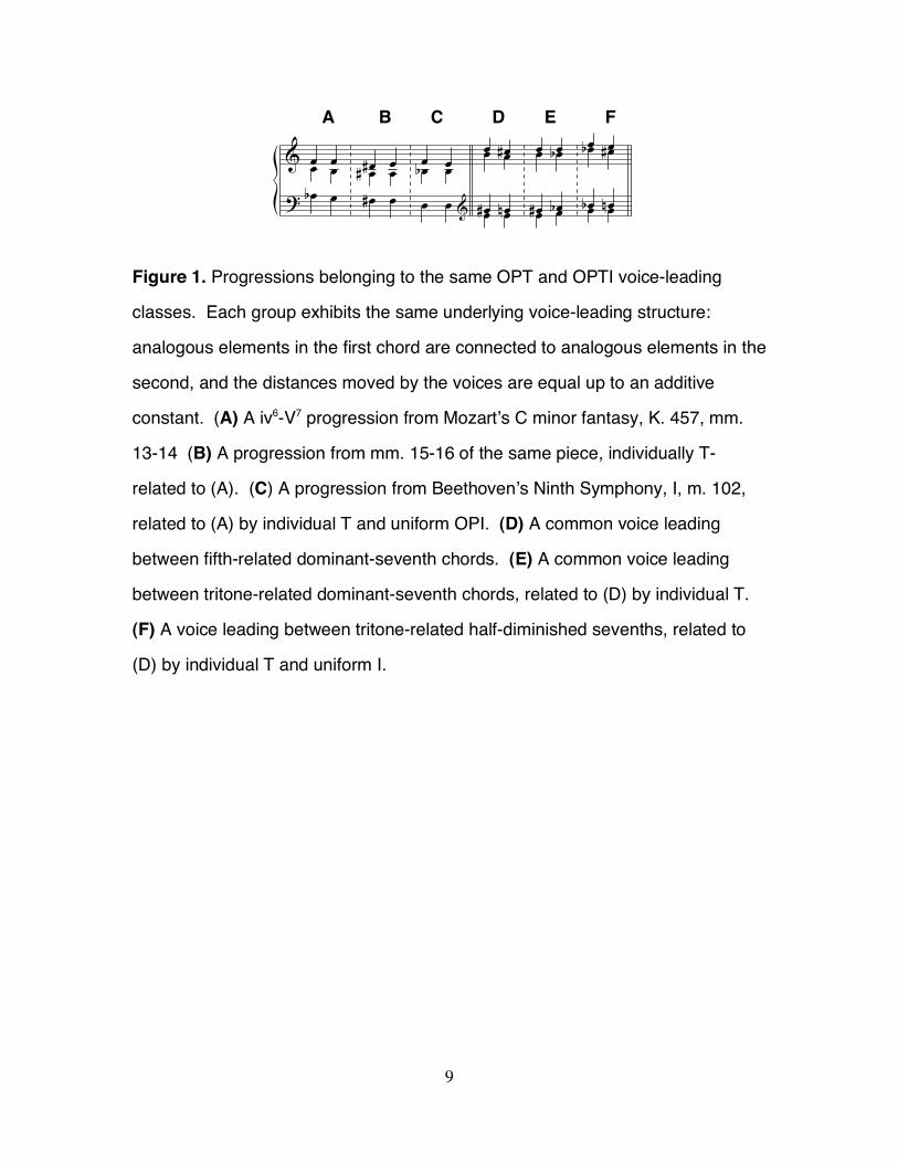
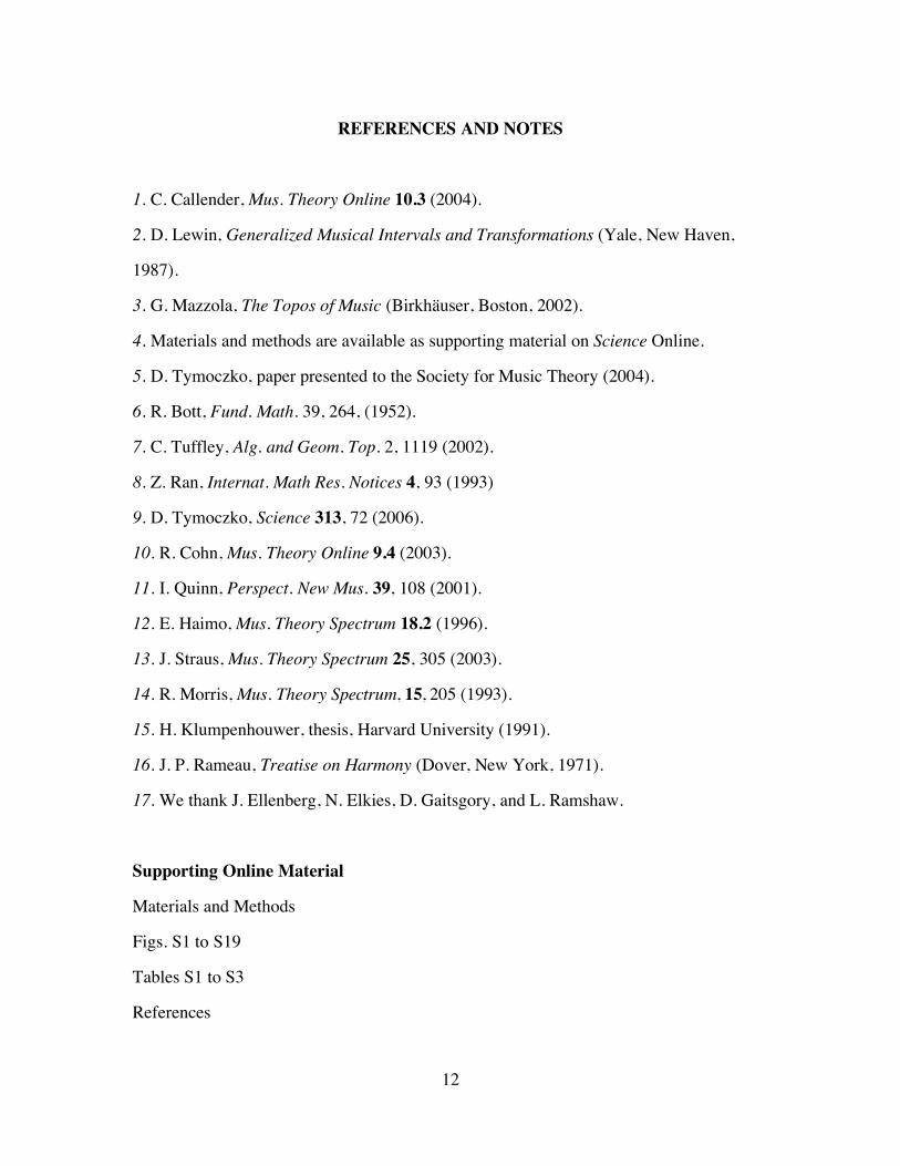
Figure 1. Progressions belonging to the same OPT and OPTI voice-leading
classes. Each group exhibits the same underlying voice-leading structure:
analogous elements in the first chord are connected to analogous elements in the
second, and the distances moved by the voices are equal up to an additive
constant. (A) A iv6-V7 progression from Mozart s C minor fantasy, K. 457, mm.
13-14 (B) A progression from mm. 15-16 of the same piece, individually T-
related to (A). (C) A progression from Beethoven s Ninth Symphony, I, m. 102,
related to (A) by individual T and uniform OPI. (D) A common voice leading
between fifth-related dominant-seventh chords. (E) A common voice leading
between tritone-related dominant-seventh chords, related to (D) by individual T.
(F) A voice leading between tritone-related half-diminished sevenths, related to
(D) by individual T and uniform I.
10
A
B
Figure 2. A. T2/S3 is a cone. B. T2/(S3 Z2) is a triangle. Numbers refer to pitch
classes, with 0 = C, 1 = Cs, etc. Points represent equivalence classes of
transpositionally (A) or transpositionally and inversionally (B) related chords.
Thus, (C, D, E) and (D, E, Fs) are both instances of 024.
11
A
014 015
026
Schoenberg
etmt
just
B
&œ
œ# œn œœ œ œ#
œ œ
Figure 3. A. The cone T2/S3 (Fig. 2A) as seen from above. The term “scale
fragment” refers to grid points in the leftmost circle: “Do, Re, Mi” is 024, “Re, Mi,
Fa” is 023, and “Mi, Fa, Sol” is 013. “Triad” refers to points in the larger circle on
the right, containing major (047), minor (037), augmented (048), and diminished
(036) chords. Different tunings of the major triad are found in the dotted circle
around 047. On the right, the equal-tempered, just, and quarter-comma
meantone triads. B. Closely-related motives at the beginning of Schoenberg s
Opus 11, no. 1. The variations define a pair of short line segments in the cone,
from 014 to 015 to 026.
12
REFERENCES AND NOTES
1. C. Callender, Mus. Theory Online 10.3 (2004).
2. D. Lewin, Generalized Musical Intervals and Transformations (Yale, New Haven,
1987).
3. G. Mazzola, The Topos of Music (Birkhäuser, Boston, 2002).
4. Materials and methods are available as supporting material on Science Online.
5. D. Tymoczko, paper presented to the Society for Music Theory (2004).
6. R. Bott, Fund. Math. 39, 264, (1952).
7. C. Tuffley, Alg. and Geom. Top. 2, 1119 (2002).
8. Z. Ran, Internat. Math Res. Notices 4, 93 (1993)
9. D. Tymoczko, Science 313, 72 (2006).
10. R. Cohn, Mus. Theory Online 9.4 (2003).
11. I. Quinn, Perspect. New Mus. 39, 108 (2001).
12. E. Haimo, Mus. Theory Spectrum 18.2 (1996).
13. J. Straus, Mus. Theory Spectrum 25, 305 (2003).
14. R. Morris, Mus. Theory Spectrum, 15, 205 (1993).
15. H. Klumpenhouwer, thesis, Harvard University (1991).
16. J. P. Rameau, Treatise on Harmony (Dover, New York, 1971).
17. We thank J. Ellenberg, N. Elkies, D. Gaitsgory, and L. Ramshaw.
Supporting Online Material
Materials and Methods
Figs. S1 to S19
Tables S1 to S3
References
1
SUPPORTING ONLINE MATERIAL TABLE OF CONTENTS
1. Notation 1 2. Chords, set classes, voice leadings and chord-progressions 2 3. Equivalence classes, quotient spaces, and music 3 4. Proto-metrics and isometries 5 5. Quotient spaces, fundamental domains, OPT, and OPTI 7 6. Voice leading in conical OPT space 10 7. Similarity between chord types 13 8. Contour 15 9. Larger equivalence classes: lines, planes, and K-nets 16 10. Supplementary Figures 20 11. Supplementary Tables 45 12. References and Notes 49
1. Notation. C4 is middle C, C5 is an octave above middle C, and so on; B3 is a semitone
below C4. R denotes the real numbers, Z the integers, Tn the n-torus, and Sn the
symmetric group of order n. Tx denotes transposition by x semitones: Tx(p) = p + x. Iy
x
denotes the reflection that maps x to y: Iyx (p) = (x + y) – p.
We use subscripts to denote equivalence classes: (x1, …, xn)F denotes the
equivalence class formed by applying the musical operations in F to the musical object
(x1, …, xn). Thus (E4, G4, C4), (G2, G3, D5, B3) (C4, E4, G4)OPTC. For progressions, we
use (x1, …, xn)F (y1, …, yn)F to denote the equivalence class resulting from individual
applications of F, and (x1, …, xn) F (y1, …, yn) to denote the equivalence class resulting
from uniform applications of F. The two notations can be combined: thus (C4, E4, G4)
OPI (C4, F4, A4)T denotes the equivalence class of progressions related to (C4, E4, G4)
(C4, F4, A4) by individual T and uniform OPI (S1).
Note that there is a difference between the O and T operations: T operations send
the pitches (x1, …, xn) to (x1 + c, …, xn + c), for some real number c, while O operations
send (x1, …, xn) to (x1 + 12i1, …, xn + 12in) for some collection of integers ij. (These
definitions reflect musical practice.) One could say that T acts “uniformly” on the notes
in an object, while O acts “individually.” In this paper, however, we use the terms
2
“uniform” and “individual” only for progressions. Both O and T can apply to
progressions either uniformly or individually.
The term “scalar transposition,” used briefly in the main text, refers to
transposition or translation along a scale. Given the ascending circular ordering of pitch-
classes (C, D, E, F, G, A, B, [C]), scalar transposition by one ascending step sends
(C, D, E) to (D, E, F), shifting every note upward by one scale tone. We can interpret a
scale as defining a metric according to which adjacent scale tones are one “unit” apart;
scalar transposition is just translation relative to this metric (S2).
2. Chords, set classes, voice leadings and chord-progressions. A “pitch class” is an
equivalence class of one-note objects related by O. Pitch classes can be designated by
letter names like “C” and “A” without an Arabic subscript identifying a particular octave.
A “chord” is an equivalence class of objects related by OPC. Chords can be identified
with unordered sets of pitch classes, and are often called “sets” in contemporary theory.
A “chord type” (or “transpositional set class”) is an equivalence class of objects related
by OPTC. Terms like “major chord” and “dominant seventh chord” refer to chord types
(S3). A “set class” is an equivalence class of objects related by OPTIC. Set classes have
long been central to music theory: for example, Rameau used the term “perfect chord” to
refer to the set class containing major and minor triads (S4).
The progression (C4, E4, G4) (C4, F4, A4) defines three melodic voices that move
C4 to C4, E4 to F4, and G4 to A4 (Fig. S2A). Theorists are often uninterested in the overall
order of the voices. A voice leading in pitch space is an equivalence class of
progressions under uniform permutation: (C4, E4, G4) (C4, F4, A4) and (E4, G4, C4)
(F4, A4, C4) are instances of the same voice leading in pitch space, (C4, E4, G4)P
(C4, F4, A4). Theorists also find it useful to abstract away from the particular octave in
which voices appear. A voice leading in pitch-class space is an equivalence class of
progressions under uniform permutation and octave shifts: (C4, E4, G4) (C4, F4, A4) and
(E2, C5, G3) (F2, C5, A3) represent the same voice leading in pitch class space,
(C4, E4, G4)OP
(C4, F4, A4). Here, C moves to C by 0 semitones, E moves to F by 1
semitone, and G moves to A by 2 semitones.
3
A “chord-progression” is a progression with no implied mappings between its
objects’ elements. (Note the hyphen: chord-progressions are a particular subspecies of
progression.) Chord-progressions can be modeled as equivalence classes under
individual applications of OPC: thus (C4, E4, G4) (F4, F3, A4, C5) and (E4, C4, G5)
(F4, C4, A5) are instances of the chord-progression (C4, E4, G4)OPC (F4, A4, C5)OPC.
Intuitively, chord-progressions represent sequences of chords considered as indivisible,
harmonic “wholes,” while voice leadings represent specific connections between the
notes of successive chords. The difference between chord-progressions and voice
leadings illustrates the difference between individual and uniform applications of the
OPTIC operations.
Hugo Riemann classified triadic chord-progressions by uniform TI and individual
OPC (S5). Thus he used a single term, Quintschritt, to label the progressions (C4, E4, G4)
(G4, B4, D5) and (C4, Ef4, G4) (F3, Af3, C4), even though the first progression ascends
by fifth, while the second descends by fifth. We can generalize Riemann’s terminology
by saying that two progressions are dualistically equivalent if they are related by uniform
TI and individual OPC.
3. Equivalence classes, quotient spaces, and music. A number of theorists (S6–7) have
investigated the role of symmetries and equivalence classes in music theory. The present
paper builds on this previous work in several ways: first, it describes a collection of five
OPTIC transformations intrinsic to traditional musical discourse; second, it shows how to
apply these transformations to progressions as well as individual objects; third, it
identifies a particular class of quotient spaces in which natural geometrical structures
correspond to familiar musical objects; fourth, it describes the specific geometry,
topology, and musical interpretation of the resulting spaces; and fifth, it uses voice
leading to reinterpret a variety of other music-theoretical terms, such as similarity,
contour, and K-nets.
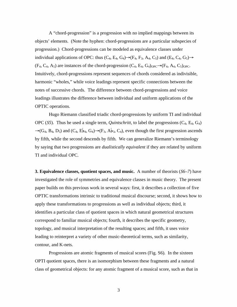
Progressions are atomic fragments of musical scores (Fig. S6). In the sixteen
OPTI quotient spaces, there is an isomorphism between these fragments and a natural
class of geometrical objects: for any atomic fragment of a musical score, such as that in
4
Figure S6A, there is a unique line segment (or pair of points) in the quotient, such as that
in Figure S6C; conversely, for any line segment (or pair of points) in the quotient, there
will be a corresponding equivalence class of atomic fragments.
This is not true of musical quotient spaces in general. For example, suppose one
were to model equal-tempered pitch-classes as elements of the cyclic group Z12 and two-
note chords as points in the discrete quotient space ((Z12)2 – Z12)/S2. (We use ((Z12)
2 –
Z12)/S2 because the music-theoretical tradition ignores “chords” with multiple copies of a
single pitch class, such as {C, C}.) Now consider the two progressions shown in Fig
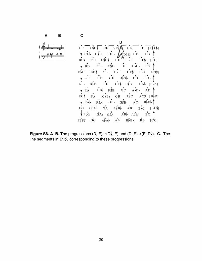
S6A-B. In two-note OP space, T2/S2, these are represented by distinct paths (Fig S6C):
one moves directly from {D, E} to {Ds, E}, while the other reflects off the space’s
singular boundary. However, the discrete space ((Z12)2 – Z12)/S2 does not distinguish
these progressions, for three reasons. First, there are no line-segments in the discrete
space. Second, chords such as {C, C} do not appear in ((Z12)2 – Z12)/S2, and hence there
is no singular boundary to “bounce off.” Thus, the line segment (D, E) (E, Ds) is not
represented even in T2/S2 – T
1, the continuous noncompact Möbius strip representing
two-note chords with two distinct pitch classes. Third, the path in Figure S6B intersects
the singular boundary at a point with non-integral coordinates: thus, even if we were to
use the space (Z12)2/S2, which has singular points, and even if we were to define a
discrete analogue to the notion of “line segment,” it would still be awkward to model this
path.
Other musical quotient spaces create analogous complications (S8). In general,
the most transparent isomorphism between familiar musical events and familiar
geometrical concepts is obtained when pitches are modeled using real numbers, and when
multisets such as {C, C, E, G} are included. Furthermore, as we will see in the next
section, distances in the resulting spaces represent voice-leading size only when the
operations that form the quotient are isometries of generic voice-leading metrics. Our
suggestion is that the OPTI spaces are interesting precisely because they satisfy these
conditions, thereby giving rise to geometrical structures with a particularly clear musical
interpretation.
5
4. Proto-metrics and isometries. There are several ways to measure musical distance.
For example one could consider the notes C3 and G4 to be close because the ratio of their
fundamental frequencies can be expressed using small whole numbers. This is an
acoustic conception of musical distance. Alternatively, one could consider the chords
(C, Cs, E, Fs)OP and (C, Cs, Ds, G)OP to be close, or even identical, since each contains
the same total collection of intervals: a semitone (C-Cs), a major second (E-Fs and Cs-
Ds), a minor third (Cs-E and C-Ds), and so on. This is an intervallic conception of
musical distance (S9). Finally, it is important to distinguish perceptual models of musical
distance, which focus on the experience of hearing music, from conceptual models,
which attempt to describe more abstract cognitive structures musicians use to understand
or compose music.
In this paper, we explore a conceptual model that measures distance melodically,
using distance in log-frequency space (S10–11). Melodic distance is important for two
reasons: first, because large melodic leaps can often be difficult to sing or play; and
second, because short melodic distance facilitates auditory streaming, or the separation of
the sound-stimulus into independent melodic lines (S12–13). As a result Western
composers typically move from chord to chord in a way that minimizes the log-frequency
distance traveled by each voice (S2, S14–16). What complicates matters is that Western
polyphonic music involves multiple melodies at one time. Thus if one wants to measure
the melodic distance between chords, it is necessary to determine whether the voice
leading (C4, E4, G4)OP
(Df4, F4, Af4), which moves three voices by one semitone each,
is larger or smaller than (C4, E4, G4)OP
(C4, E4, A4), which moves one voice by two
semitones. The problem is that there is no obvious answer to this question: instead, there
are a number of reasonable but subtly different ways to measure voice leading.
Let A B (a1, a2, …, an) (b1, b2, …, bn) be a progression of two n-note
musical objects. We define this progression’s displacement multiset as {|a1 – b1|, …,
|an – bn|}, or dm(A B). A proto-metric is a preorder over multisets of nonnegative reals
satisfying what Tymoczko (S2) calls the “distribution constraint”:
{x1 + c, x2, ..., xn} {x1, x2 + c, ..., xn} {x1, x2, ..., xn}, for x1 > x2, c > 0
6
A proto-metric allows comparison of some distances in Rn, thereby endowing the space
with more-than-topological, but less-than-geometrical structure. It is argued in (S2) that
any music-theoretically reasonable method of measuring voice leading must be consistent
with the distribution constraint, since otherwise voice leadings with “voice crossings”
would be smaller than their naturally uncrossed alternatives. Furthermore, every existing
music-theoretical method of measuring voice leading satisfies the constraint.
Uniform application of the OPTI symmetries preserves the displacement multiset
{|a1 – b1|, …, |an – bn|} and hence preserves the proto-metric: if F is any OPTI operation,
then dm(F(A) F(B)) = dm(A B); thus A B is smaller than C D if and only if
F(A) F(B) is smaller than F(C) F(D). Consequently, quotients of the OPTI
operations inherit the proto-geometrical structure of the parent space Rn. For a large
class of suitable metrics, this means that distance in the quotient space will correspond to
the length of the shortest line-segment between two points, as measured using the
quotient metric (S17). Musically, this means that we can use voice-leading size to
measure distance between chord-types.
The C operation does not have this property, since it identifies the voice leading
C4 G4, whose displacement multiset is {7}, with the voice leading (C4, C4, C4)
(G4, G4, G4), whose displacement multiset is {7, 7, 7}. According to most music-
theoretical metrics {7} and {7, 7, 7} do not have the same size: this is because it takes
less musical “work” to move one voice by seven semitones than to move three voices by
seven semitones. Consequently, the C operation is not an isometry of proto-metrics in
general (S18).
This problem arises even in contexts that do not involve note duplication.
Consider a chord A consisting of a large number of distinct pitches infinitesimally close
to C4, and a chord B consisting of a large number of distinct pitches infinitesimally close
to G4. According to standard metrics of voice leading size, the voice leadings taking the
pitches of A to C4 and the pitches of B to G4 are infinitesimally small; the triangle
inequality therefore requires that the voice leading A B should be approximately the
same size as the voice leading C4 G4. But any voice leading from A to B must move a
7
large number of voices by approximately seven semitones each, and (according to many
standard metrics) is considerably larger than the voice leading C4 G4 (S19). Thus we
must either abandon the triangle inequality or abandon the claim that A B is
significantly larger than C4 G4. Either way, we abandon the idea that voice-leading size
corresponds to something like distance in the quotient space.
It follows that the C spaces are not ideal for studying voice leading, since we
cannot use distance in the C spaces to explain the efficient voice-leading possibilities
between chords. However, C spaces may usefully model similarity between chord types,
as we will discuss in §6. In this context, violations of the triangle inequality do not
necessarily present a serious music-theoretical obstacle.
5. Quotient spaces, fundamental domains, OPT, and OPTI. A quotient space is
formed by identifying (or “gluing together”) all points in a parent space related by some
collection of operations F. A fundamental domain for F is a region in the parent space
satisfying two constraints: first, every point in the entire space is related by operations in
F to some point in the region; and second, no two points in the interior of the region are
related by operations in F. (Typically, fundamental domains are also taken to be
connected regions with a straightforward geometrical structure, but this is largely a
matter of convenience.) The fundamental domain is analogous to a single “tile” of a
piece of wallpaper.
The quotient space can be formed from the fundamental domain by gluing
together all points on the fundamental domain’s boundary that are related by operations
in F. For example, the (closed) upper half plane is a fundamental domain for 180°
rotations in R2, since any point in the interior of the upper half-plane is related by 180°
rotation to a point in the lower half plane (Figure S7). Since points on the positive x axis
are related by 180° rotation to points on the negative x axis, they must be glued together
to form the quotient space. The result of this identification is a cone, as shown in Figure
S7.
8
We begin with Rn, the space of n-note musical objects. The O operation
transforms Rn into the n-torus T
n. Musically, the most useful fundamental domain for the
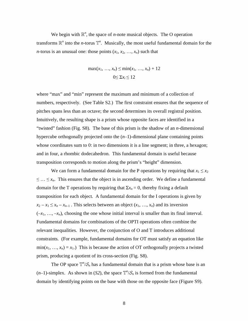
n-torus is an unusual one: those points (x1, x2, …, xn) such that
max(x1, …, xn) min(x1, …, xn) + 12
0 xi 12
where “max” and “min” represent the maximum and minimum of a collection of
numbers, respectively. (See Table S2.) The first constraint ensures that the sequence of
pitches spans less than an octave; the second determines its overall registral position.
Intuitively, the resulting shape is a prism whose opposite faces are identified in a
“twisted” fashion (Fig. S8). The base of this prism is the shadow of an n-dimensional
hypercube orthogonally projected onto the (n–1)-dimensional plane containing points
whose coordinates sum to 0: in two dimensions it is a line segment; in three, a hexagon;
and in four, a rhombic dodecahedron. This fundamental domain is useful because
transposition corresponds to motion along the prism’s “height” dimension.
We can form a fundamental domain for the P operations by requiring that x1 x2
… xn. This ensures that the object is in ascending order. We define a fundamental
domain for the T operations by requiring that xn = 0, thereby fixing a default
transposition for each object. A fundamental domain for the I operations is given by
x2 – x1 xn – xn–1 . This selects between an object (x1, …, xn) and its inversion
(–x1, …, –xn), choosing the one whose initial interval is smaller than its final interval.
Fundamental domains for combinations of the OPTI operations often combine the
relevant inequalities. However, the conjunction of O and T introduces additional
constraints. (For example, fundamental domains for OT must satisfy an equation like
min(x1, …, xn) = x1.) This is because the action of OT orthogonally projects a twisted
prism, producing a quotient of its cross-section (Fig. S8).
The OP space Tn/Sn has a fundamental domain that is a prism whose base is an
(n–1)-simplex. As shown in (S2), the space Tn/Sn is formed from the fundamental
domain by identifying points on the base with those on the opposite face (Figure S9).
9
(The rectangular boundaries of the fundamental domain in Figure S9A are singular
orbifold points, a matter we will disregard in the following discussion.) This
identification involves a “twist”—a rigid transformation cyclically permuting the
simplex’s vertices. OPT space Tn–1
/Sn is the orthogonal projection of this space along the
direction of transposition, and is therefore the (n–1)-simplex modulo the “twist.” This
space can be visualized as a cone over a quotient of the (n–2)-sphere, since the simplex is
homeomorphic to a ball, which is itself a cone over the sphere. (Note, however, that this
“cone” will contain additional orbifold points with complicated topology: the vertex, the
base, and for chords with a nonprime number of notes, points on other layers as well.)
When n is prime, the group generated by cyclic permutation has no fixed points and the
base of Tn–1
/Sn is a lens space (S20). Mathematically, transposition induces a foliation of
chord space (Tn/Sn), with chord-type space (T
n–1/Sn) being the “leaf space” of the
foliation.
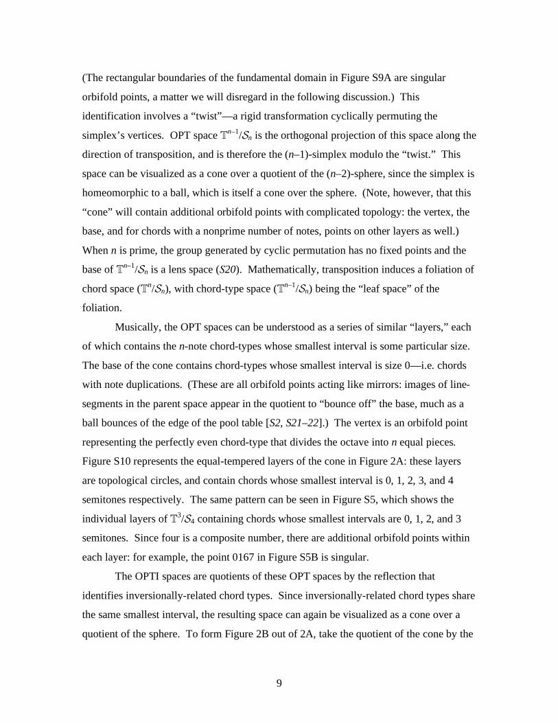
Musically, the OPT spaces can be understood as a series of similar “layers,” each
of which contains the n-note chord-types whose smallest interval is some particular size.
The base of the cone contains chord-types whose smallest interval is size 0—i.e. chords
with note duplications. (These are all orbifold points acting like mirrors: images of line-
segments in the parent space appear in the quotient to “bounce off” the base, much as a
ball bounces of the edge of the pool table [S2, S21–22].) The vertex is an orbifold point
representing the perfectly even chord-type that divides the octave into n equal pieces.
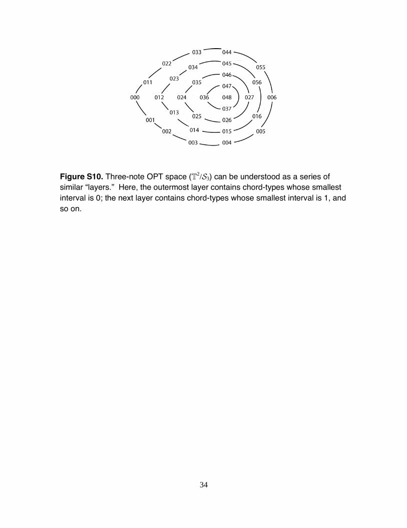
Figure S10 represents the equal-tempered layers of the cone in Figure 2A: these layers
are topological circles, and contain chords whose smallest interval is 0, 1, 2, 3, and 4
semitones respectively. The same pattern can be seen in Figure S5, which shows the
individual layers of T3/S4 containing chords whose smallest intervals are 0, 1, 2, and 3
semitones. Since four is a composite number, there are additional orbifold points within
each layer: for example, the point 0167 in Figure S5B is singular.
The OPTI spaces are quotients of these OPT spaces by the reflection that
identifies inversionally-related chord types. Since inversionally-related chord types share
the same smallest interval, the resulting space can again be visualized as a cone over a
quotient of the sphere. To form Figure 2B out of 2A, take the quotient of the cone by the
10
reflection that fixes 048 (the vertex), 000 (the “kink” in the base) and 006 (the point on
the base antipodal to the kink), as shown in Figure S9. This produces the triangle in
Figure 2B and S9E—a “cone” over the line segment from 000 to 006. Similarly, to form
Figure S5E out of Figure S5A identify each point with its geometrical inversion through
the center of the square. Three-note OPTI space was first described by Callender (S22)
while four-note OPTI space was partially described by Cohn (S23, fig. S4F), and
described more completely in unpublished work by Quinn. Interested readers can
explore these spaces further by downloading “ChordGeometries,” a free computer
program written by Dmitri Tymoczko (S24).
6. Voice leading, orbifold points, and conical OPT space. The description of OPT and
OPTI spaces as cones allows for a concise reformulation of one of the central conclusions
in (S2), that “nearly even” chords can be linked to their transpositions by efficient voice
leading. In conical OPT space, the “unevenness” of a chord corresponds to its distance
from the vertex. Nearly even chords can be linked to their transpositions by efficient
voice leading because short line segments near the vertex of a cone can self-intersect.
These self-intersecting line segments represent progressions combining harmonic
consistency (since they link transpositionally related chords) with efficient voice leading
(since they are short), two cardinal desiderata of traditional Western music (S2). Thus a
fact of central importance to Western music reduces to a familiar feature of the geometry
of cones.
In fact, there is a more general relation between voice leading and orbifold points.
To explore this, we will temporarily adopt the Euclidean voice-leading metric—
mathematically very convenient, because the voice leading A Tx(B) (a0, …, an–1)
(b0 + x, …, bn–1 + x) is minimized when A and Tx(B) sum to the same value.
Furthermore, from the standpoint of the distribution constraint, the Euclidean metric is
nicely intermediate between the extremal cases of L1 and L (S25). Thus, results that are
exactly true in the Euclidean case will be approximately true for other metrics satisfying
the distribution constraint, with the accuracy of the approximation controlled by the
particular metric in question.
11
We begin with a simple theorem of Euclidean geometry. Let A be any vector and
let Bi be a collection of n vectors that add to zero. The sum of the squared Euclidean
distances |Bi – A| is equal to
|Bi – A|
2 = |B
i |2 – 2 (B
i • A) + n|A|
2 = |B
i|2 + n|A|
2
since Bi = 0. When the B
i are all the same length, |B|, we have |A|
2 + |B|
2 = |A – B
i|2/n.
We now examine three cases where this fact has an interesting music-theoretical
interpretation. In each case, the lengths |A|2 and |B|
2 will represent intrinsic properties of
chords A and B (such as their “evenness” or “spread”) while |A – Bi|2/n will represent
something about the voice-leading possibilities between them.
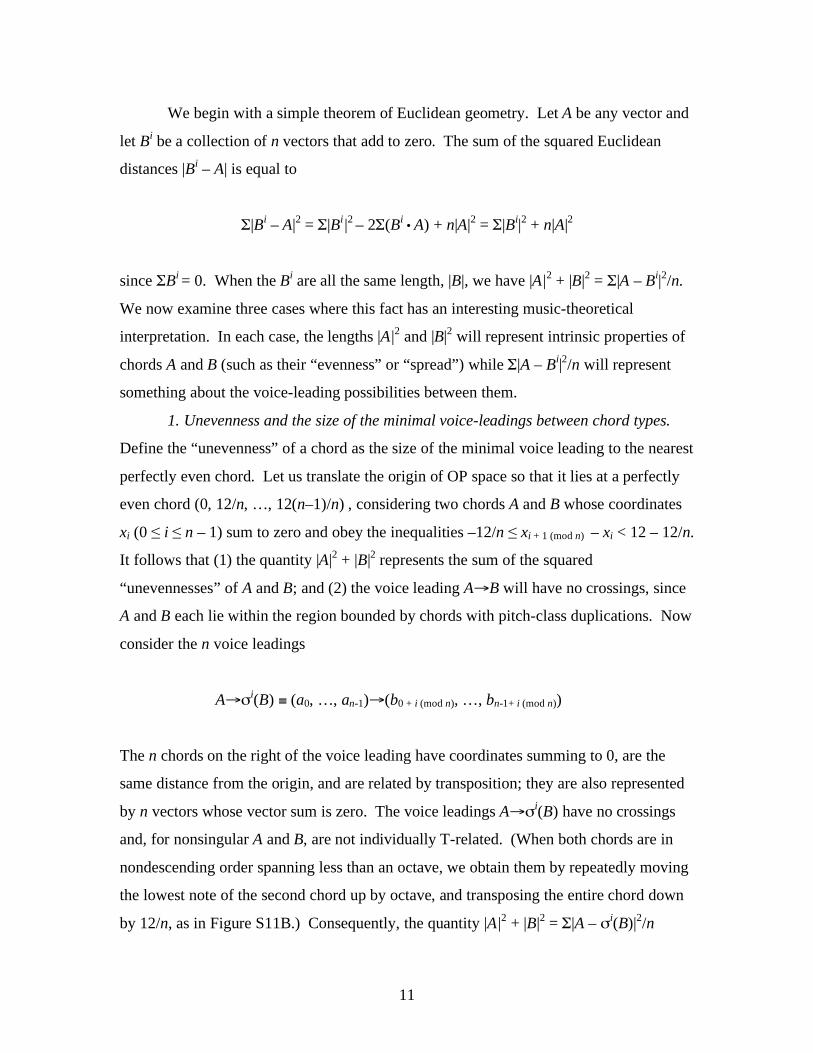
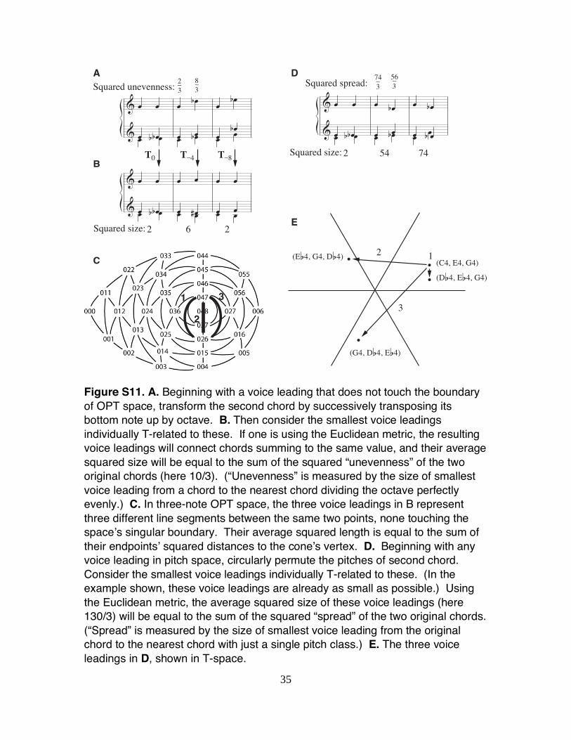
1. Unevenness and the size of the minimal voice-leadings between chord types.
Define the “unevenness” of a chord as the size of the minimal voice leading to the nearest
perfectly even chord. Let us translate the origin of OP space so that it lies at a perfectly
even chord (0, 12/n, …, 12(n–1)/n) , considering two chords A and B whose coordinates
xi (0 i n – 1) sum to zero and obey the inequalities –12/n xi + 1 (mod n) – xi < 12 – 12/n.
It follows that (1) the quantity |A|2 + |B|
2 represents the sum of the squared
“unevennesses” of A and B; and (2) the voice leading A B will have no crossings, since
A and B each lie within the region bounded by chords with pitch-class duplications. Now
consider the n voice leadings
Ai(B) (a0, …, an-1) (b0 + i (mod n), …, bn-1+ i (mod n))
The n chords on the right of the voice leading have coordinates summing to 0, are the
same distance from the origin, and are related by transposition; they are also represented
by n vectors whose vector sum is zero. The voice leadings Ai(B) have no crossings
and, for nonsingular A and B, are not individually T-related. (When both chords are in
nondescending order spanning less than an octave, we obtain them by repeatedly moving
the lowest note of the second chord up by octave, and transposing the entire chord down
by 12/n, as in Figure S11B.) Consequently, the quantity |A|2 + |B|
2 = |A –
i(B)|
2/n
12
represents both the sum of the chords’ squared “evennesses” and the average squared size
of the crossing-free OPT voice-leading classes between chord-types AOPT and BOPT
(Figure S11A-C). For very even chords, such as the major and minor triads of the
classical tradition, there will be multiple small crossing-free voice-leading possibilities
between their transpositions. (Recall from §4 that crossing-free voice leadings are
desirable for a number of reasons, not least because there is always a minimal voice
leading between two chords that is crossing free.) This gives composers a wealth of
contrapuntal options to choose from.
2.“Spread” and the size of crossed voice-leadings between chords. A similar
result relates the size of voice leadings with crossings to the “spread” of two chords—that
is, their distance from the perfectly clustered chord-type {0, …, 0}T. Consider chords A
and B whose coordinates xi sum to zero. If the origin is the perfectly clustered chord,
then |A|2 + |B|
2 represents the sum of the squared “spreads” of A and B. The n voice
leadings Ai(B) are now obtained by circularly permuting the notes of the second
chord without any transposition (Fig. S11D). The average squared size of these voice
leadings will be equal to the sum of the chords’ “spread.” Thus a very clustered chord
can be connected to some transposition of another very clustered chord by many different
efficient voice leadings. The result can be generalized to all permutations of chord B.
3. Inversions. Choose an inversionally symmetrical sequence of pitch classes such
that (x1, …, xn) = (c – xn, …, c – x1), and translate the origin of OT so that it lies at this
point; thus, all chords B and –B are inversionally related. The quantities |A|2 and |B|
2
represent the squared distance to the inversionally symmetrical chord at the origin. Our
result now says that the sum of these squared distances is equal to the average squared
size of the voice leadings A B and A –B. The closer A and B are to the inversionally
symmetrical chord midway between B and –B, the smaller these two voice leadings will
be.
In each of case, we find a similar relationship between voice leading and distance
from orbifold points. If we assume the Euclidean metric, we can express this relationship
in quantitative terms: the sum of the squared distances between two chords and some
particular orbifold point is equal to the average of the squared size of some musically
13
interesting collection of voice leadings between them. For an arbitrary metric obeying
the distribution constraint, there is no equivalently elegant quantitative result, but similar
relationships obtain approximately. Western composers have exploited these facts to
write progressions connecting structurally similar chords by efficient voice leading (S2).
7. Similarity among chord types. Over the last twenty years, a number of theorists have
attempted to model musical conceptions of “similarity” (or inverse distance) between
chord types. These models have been based on the intervallic conception of distance
described in §4 (S26–29), Fourier-transform-based extensions to these models (S9), the
prevalence of shared subsets (S30–33), or meta-analyses of models in these categories
(S34–35). Following Roeder (S36) and Straus (S37), we suggest an approach based on
voice leading: specifically, we propose modeling the similarity between equivalence
classes as the size of the smallest voice leading between their elements. Conceiving of
similarity in this way has a number of advantages:
1. As described in the text, this approach is consistent with the flexibility
inherent in terms such as “scale fragment,” “triad,” and “major triad.”
Furthermore, composers often do vary musical material in accordance with
this notion of similarity (Fig. 3).
2. Since this conception of similarity is consistent with aggregate physical
distance on a keyboard instrument, it is plausible that composers would be
sensitive to it.
3. This approach permits different chords to have different degrees of “self
similarity,” here measured by the size of the smallest nontrivial voice
leading from a chord-type to itself. Chord-types with a high degree of self-
similarity have played a prominent role in Western music (S2).
4. This approach generalizes naturally to continuous spaces, in such a way that
chord-types differing by imperceptible distances are judged highly similar.
Furthermore, the approach provides similarity measurements that are
independent of the underlying chromatic universe. Other similarity metrics
(S26–S35) lack these properties.
5. Unlike intervallic similarity metrics (S9, S26–S29), this approach
distinguishes “Z-related” (or nontrivially homometric) chords such as
{C, Cs, E, Fs} and {C, Cs, Ds, G} which are often thought to be dissimilar.
6. There exist a range of OPTI quotient spaces modeling different degrees of
musical abstraction. Thus, unlike other metrics (S9, S26– S29), the
14
approach itself does not require one particular set of symmetries—such as,
for example, the identification of inversionally-related chords.
7. The approach generalizes naturally to measures of voice-leading similarity,
as will be discussed shortly.
We do not assert that voice-leading-based similarity metrics represent the only coherent
approach to the problem. However, we do suggest that the seven considerations adduced
above provide good reason to explore them.
Note that when modeling judgments of chord-type similarity it may be useful to
impose C equivalence: thus we may want to consider {C, C, E} and {C, E, E} to be
identical, and to consider{B, Cs, G} to be highly similar to{C, Fs, G}. (This is because
the two chords can be linked by the voice leading (B, Cs, G, G) (C, C, Fs, G), which is
both a nonbijective voice leading from {B, Cs, G}C to {C, Fs, G}C and a bijective voice
leading from {B, Cs, G, G} to {C, C, Fs, G}.) The fact that “distances” in the resulting
C-spaces do not obey the triangle inequality should not necessarily be a cause for alarm,
as there is no reason to expect psychological similarity judgments to be metrically well-
behaved (S38).
Infinite-dimensional C space is of course quite complex. Fortunately, in most
practical situations, the goal is to model relatively coarse-grained similarity judgments:
for example, to explain straightforward processes of musical variation such as that in
Figure 3B. In these contexts, it is often sufficient to work with a finite-dimensional OPT
or OPTI space. Furthermore, choosing a specific metric of voice leading size is often
unnecessary: the distribution constraint alone ensures that (E, F, A)OPT is as close to
(G, Gs, B)OPT as any other equal-tempered transpositional set class. Thus Schoenberg’s
process of melodic variation in Figure 3 is a series of minimal changes in equal-tempered
OPTIC space—no matter what measure of voice-leading size we prefer.
We can also use voice leading to measure the similarity of musical progressions:
one compares two-element progressions by parallel-transporting them so that they start at
the same point in the relevant quotient space; the distance between their endpoints
represents their relatedness. Figure S12A identifies two pairs of voice leadings in
Brahms’s Op. 116, no. 5, while Figure S12B models these voice leadings in T2/S2. If we
parallel transport the vectors in the most direct way (S12B), they nearly though not
15
exactly coincide. This reflects the intuitive sense that the gestures are closely, but not
exactly, related. However, the vectors can also be parallel transported so that they
exactly coincide (S12D), revealing a non-obvious symmetry in Brahms’s piece. The
symmetry is hard to spot in the musical notation, though it is obvious in the geometrical
representation. It is also fairly easy to hear: X1 and Y2 contain contrary motion where
both voices move by semitone, while X2 and Y1 contain contrary motion where one
voice moves by one semitone and the other moves by two semitones. Since the two pairs
of vectors are related by reflection, the figure also illustrates the Möbius strip’s
nonorientability.
8. Contour. T-space is divided into regions whose points share the same contour, or
ordinal ranking of their elements in pitch space. Figure S13 illustrates the three-
dimensional case, showing that the six regions are described by inequalities of the form
x (1) < x (2) < x (3) where is a permutation. Music theorists have used these inequalities
to define equivalence classes, treating objects as contour-equivalent if they belong to the
same region (Fig. S13B) (S39). Elizabeth West Marvin has defined a “similarity metric”
for contours, equivalent (to within a linear function) to Kendall’s tau rank correlation
coefficient (S40–41). Geometrically, Marvin’s similarity metric counts the number of
half-spaces xi < xj containing both contours (Fig. S13C), divided by the total number of
sharable half-spaces (S42). The similarity between contours is a linearly decreasing
function of the smallest number of hyperplanes that must be traversed in moving between
their respective contour regions (Figure S13D).
Traditional models of musical contour sometimes deliver counterintuitive results.
For example, the passages in Figures S14A-B are contour-equivalent, since they both
begin with their lowest note, move to their highest note, and end with a note between the
first two. However, the resemblance between S14A and C is in some ways more striking
than that between A and B: the lowest two notes of A and C are quite close together,
which makes the difference in contour seem relatively unimportant. By contrast, since
the middle note of B is close to its upper note, its contour intuitively seems dissimilar to
that of A, even though they both exemplify the sequence low-high-middle. One can
16
capture these intuitions by individuating contours more finely, representing them as
normalized vectors in T space. Figure S14D shows that the vector representing A is
closer to that of C than that of B.
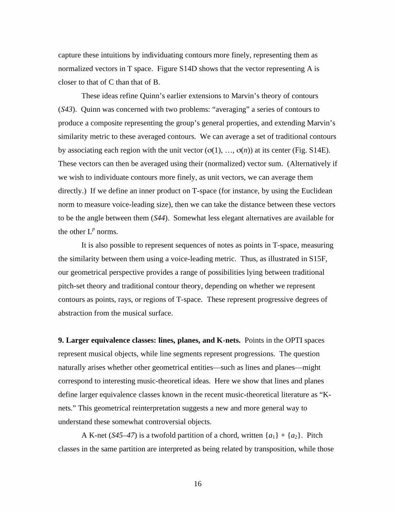
These ideas refine Quinn’s earlier extensions to Marvin’s theory of contours
(S43). Quinn was concerned with two problems: “averaging” a series of contours to
produce a composite representing the group’s general properties, and extending Marvin’s
similarity metric to these averaged contours. We can average a set of traditional contours
by associating each region with the unit vector ( (1), …, (n)) at its center (Fig. S14E).
These vectors can then be averaged using their (normalized) vector sum. (Alternatively if
we wish to individuate contours more finely, as unit vectors, we can average them
directly.) If we define an inner product on T-space (for instance, by using the Euclidean
norm to measure voice-leading size), then we can take the distance between these vectors
to be the angle between them (S44). Somewhat less elegant alternatives are available for
the other Lp norms.
It is also possible to represent sequences of notes as points in T-space, measuring
the similarity between them using a voice-leading metric. Thus, as illustrated in S15F,
our geometrical perspective provides a range of possibilities lying between traditional
pitch-set theory and traditional contour theory, depending on whether we represent
contours as points, rays, or regions of T-space. These represent progressive degrees of
abstraction from the musical surface.
9. Larger equivalence classes: lines, planes, and K-nets. Points in the OPTI spaces
represent musical objects, while line segments represent progressions. The question
naturally arises whether other geometrical entities—such as lines and planes—might
correspond to interesting music-theoretical ideas. Here we show that lines and planes
define larger equivalence classes known in the recent music-theoretical literature as “K-
nets.” This geometrical reinterpretation suggests a new and more general way to
understand these somewhat controversial objects.
A K-net (S45–47) is a twofold partition of a chord, written {a1} + {a2}. Pitch
classes in the same partition are interpreted as being related by transposition, while those
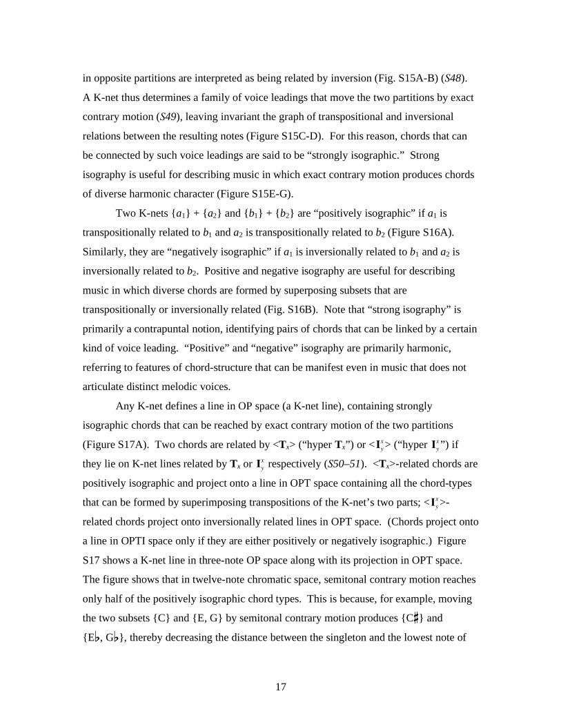
17
in opposite partitions are interpreted as being related by inversion (Fig. S15A-B) (S48).
A K-net thus determines a family of voice leadings that move the two partitions by exact
contrary motion (S49), leaving invariant the graph of transpositional and inversional
relations between the resulting notes (Figure S15C-D). For this reason, chords that can
be connected by such voice leadings are said to be “strongly isographic.” Strong
isography is useful for describing music in which exact contrary motion produces chords
of diverse harmonic character (Figure S15E-G).
Two K-nets {a1} + {a2} and {b1} + {b2} are “positively isographic” if a1 is
transpositionally related to b1 and a2 is transpositionally related to b2 (Figure S16A).
Similarly, they are “negatively isographic” if a1 is inversionally related to b1 and a2 is
inversionally related to b2. Positive and negative isography are useful for describing
music in which diverse chords are formed by superposing subsets that are
transpositionally or inversionally related (Fig. S16B). Note that “strong isography” is
primarily a contrapuntal notion, identifying pairs of chords that can be linked by a certain
kind of voice leading. “Positive” and “negative” isography are primarily harmonic,
referring to features of chord-structure that can be manifest even in music that does not
articulate distinct melodic voices.
Any K-net defines a line in OP space (a K-net line), containing strongly
isographic chords that can be reached by exact contrary motion of the two partitions
(Figure S17A). Two chords are related by <Tx> (“hyper Tx”) or <Iyx> (“hyper Iy
x”) if
they lie on K-net lines related by Tx or Iyx respectively (S50–51). <Tx>-related chords are
positively isographic and project onto a line in OPT space containing all the chord-types
that can be formed by superimposing transpositions of the K-net’s two parts; <Iyx>-
related chords project onto inversionally related lines in OPT space. (Chords project onto
a line in OPTI space only if they are either positively or negatively isographic.) Figure
S17 shows a K-net line in three-note OP space along with its projection in OPT space.
The figure shows that in twelve-note chromatic space, semitonal contrary motion reaches
only half of the positively isographic chord types. This is because, for example, moving
the two subsets {C} and {E, G} by semitonal contrary motion produces {Cs} and
{Ef, Gf}, thereby decreasing the distance between the singleton and the lowest note of
18
the minor third by two (S52). Consequently, in equal-tempered chromatic universes of
even cardinality, chords can be positively isographic even though no two of their (equal-
tempered) transpositions are strongly isographic. Remarkably, the traditional definition
of “positive isography” reflects this, even though the theory of K-nets was developed
without reference to geometry.
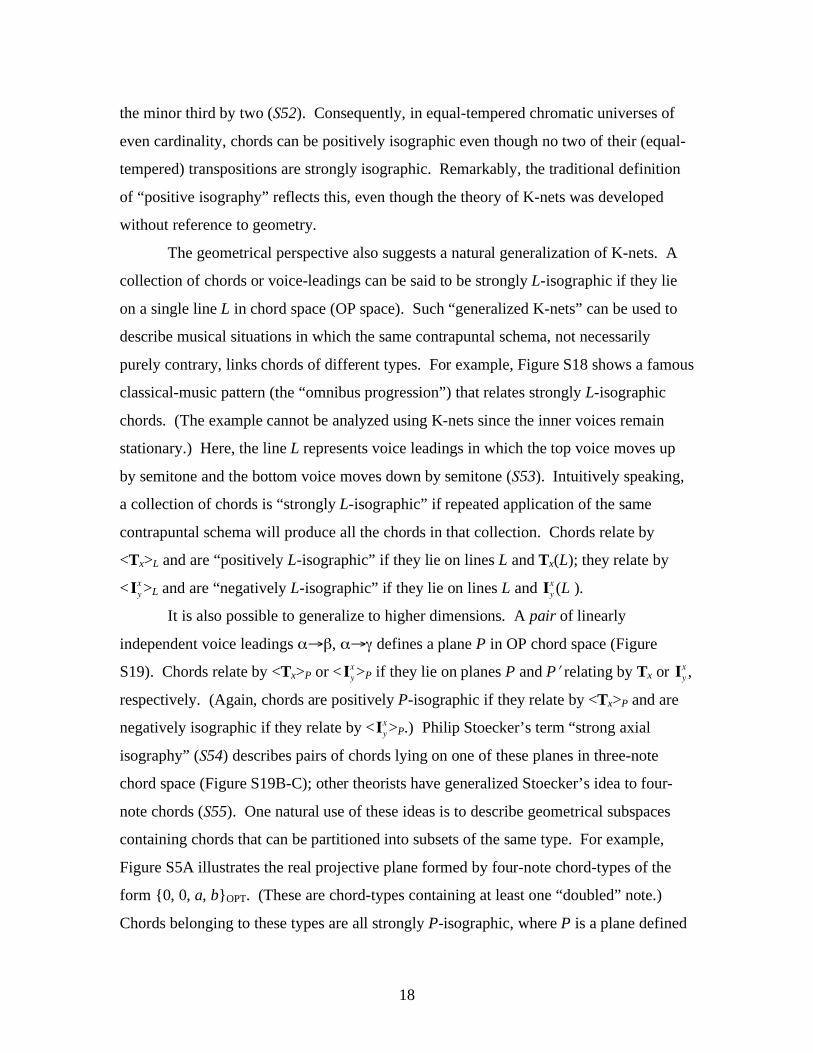
The geometrical perspective also suggests a natural generalization of K-nets. A
collection of chords or voice-leadings can be said to be strongly L-isographic if they lie
on a single line L in chord space (OP space). Such “generalized K-nets” can be used to
describe musical situations in which the same contrapuntal schema, not necessarily
purely contrary, links chords of different types. For example, Figure S18 shows a famous
classical-music pattern (the “omnibus progression”) that relates strongly L-isographic
chords. (The example cannot be analyzed using K-nets since the inner voices remain
stationary.) Here, the line L represents voice leadings in which the top voice moves up
by semitone and the bottom voice moves down by semitone (S53). Intuitively speaking,
a collection of chords is “strongly L-isographic” if repeated application of the same
contrapuntal schema will produce all the chords in that collection. Chords relate by
<Tx>L and are “positively L-isographic” if they lie on lines L and Tx(L); they relate by
< Iyx>L and are “negatively L-isographic” if they lie on lines L and Iy
x (L ).
It is also possible to generalize to higher dimensions. A pair of linearly
independent voice leadings , defines a plane P in OP chord space (Figure
S19). Chords relate by <Tx>P or < Iyx>P if they lie on planes P and P relating by Tx or Iy
x ,
respectively. (Again, chords are positively P-isographic if they relate by <Tx>P and are
negatively isographic if they relate by <Iyx>P.) Philip Stoecker’s term “strong axial
isography” (S54) describes pairs of chords lying on one of these planes in three-note
chord space (Figure S19B-C); other theorists have generalized Stoecker’s idea to four-
note chords (S55). One natural use of these ideas is to describe geometrical subspaces
containing chords that can be partitioned into subsets of the same type. For example,
Figure S5A illustrates the real projective plane formed by four-note chord-types of the
form {0, 0, a, b}OPT. (These are chord-types containing at least one “doubled” note.)
Chords belonging to these types are all strongly P-isographic, where P is a plane defined
19
by voice leadings (0, 0, a, b) (0, 0, a + , b) and (0, 0, a, b) (0, 0, a, b + ). Such
spaces can be useful in analyzing music where composers create chords by
superimposing sonorities of three fixed types.
K-nets are a notoriously difficult and even controversial topic (S56). There are,
perhaps, four reasons for this. First, previous discussion of K-nets used algebraic
language to describe objects that are more easily understood geometrically: lines and
planes in OP, OPT, and OPTI space. Second, previous discussions treat a special case of
a much more general phenomenon, considering only some of the lines and planes in the
relevant quotient spaces. Third, theorists have investigated K-nets in discrete 12-note
musical space, where the underlying relation between strong and positive isography is
obscured. And fourth, traditional theorists labeled the “hyper” transpositions and
inversions in ways that obscure their relation to ordinary transposition and inversion; as a
result, comparisons between these two forms of “transposition” are sometimes
problematic (S50, S51, S56). We hope that our geometrical reinterpretation of these
music-theoretical constructions leads to greater understanding of both their utility and
their limitations.
20
&
œœ
œ
&
&
œ
œ
œ
œ
œ
œ
œ
œ
œ
?
œ
œ
œ&
œ
œ
œ
œ
œ
œ
œ
œ#
œ
œ
œ#
œ
œ
œb
œ
œ
œb
œ
&
œ œœ
œ
&
&
œ
œ
œ
œ
M
A B C D E F G H I J K L
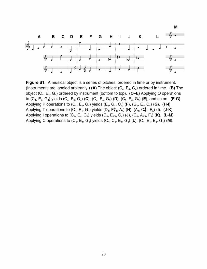
Figure S1. A musical object is a series of pitches, ordered in time or by instrument. (Instruments are labeled arbitrarily.) (A) The object (C4, E4, G4) ordered in time. (B) The object (C4, E4, G4) ordered by instrument (bottom to top). (C–E) Applying O operations to (C4, E4, G4) yields (C4, E5, G4) (C), (C4, E4, G3) (D), (C3, E4, G5) (E), and so on. (F-G) Applying P operations to (C4, E4, G4) yields (E4, G4, C4) (F), (G4, E4, C4) (G). (H-I) Applying T operations to (C4, E4, G4) yields (D4, Fs4, A4) (H), (A4, Cs4, E5) (I). (J-K) Applying I operations to (C4, E4, G4) yields (G4, Ef4, C4) (J), (C5, Af4, F4) (K). (L-M) Applying C operations to (C4, E4, G4) yields (C4, C4, E4, G4) (L), (C4, E4, E4, G4) (M).
21
&
&
&
œ œ
œ œ
œ œ
?
œ œ
œ œ
œ œ&
œ
œ
œ
œ
œ
œ
œ œ
œ œ
œ œ
œ œ
œ
œ
œœ
œ œ
œ# œ
œ œ
œ œ#
œ œ
œ œ
œ œb
œb œ
œ œ
œ
œb
œ œ
œ
œb
œ œ
œ œ
œ œ
œ œ
œ œ
œ
œ
œ œ
œ œ
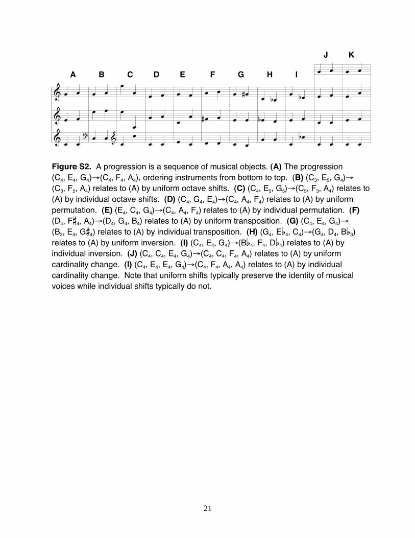
J K A B C D E F G H I Figure S2. A progression is a sequence of musical objects. (A) The progression (C4, E4, G4) (C4, F4, A4), ordering instruments from bottom to top. (B) (C3, E5, G4)
(C3, F5, A4) relates to (A) by uniform octave shifts. (C) (C4, E5, G5) (C5, F3, A4) relates to (A) by individual octave shifts. (D) (C4, G4, E4) (C4, A4, F4) relates to (A) by uniform permutation. (E) (E4, C4, G4) (C4, A4, F4) relates to (A) by individual permutation. (F) (D4, Fs4, A4) (D4, G4, B4) relates to (A) by uniform transposition. (G) (C4, E4, G4)
(B3, E4, Gs4) relates to (A) by individual transposition. (H) (G4, Ef4, C4) (G4, D4, Bf3) relates to (A) by uniform inversion. (I) (C4, E4, G4) (Bf4, F4, Df4) relates to (A) by individual inversion. (J) (C4, C4, E4, G4) (C4, C4, F4, A4) relates to (A) by uniform cardinality change. (I) (C4, E4, E4, G4) (C4, F4, A4, A4) relates to (A) by individual cardinality change. Note that uniform shifts typically preserve the identity of musical voices while individual shifts typically do not.
22
first note
seco
nd n
ote
(a, b) (a + 12, b)
(a + 12, b + 12)(a, b + 12)
trans
posit
ion
contains pairs
of pitches summing to 0
first note
seco
nd n
ote
(a, b)
(a/2 – b/2, b/2 – a/2)
first note
seco
nd n
ote
(a, b)
(–a, –b)
cont
ains
pairs
of pi
tches
(c, c
)
first note
(a, b)
(b, a)
seco
nd n
ote
A B
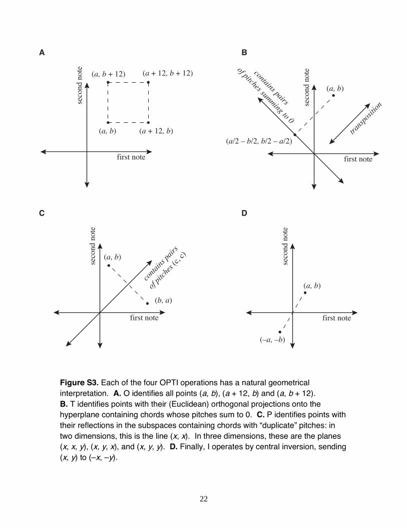
C D
Figure S3. Each of the four OPTI operations has a natural geometrical interpretation. A. O identifies all points (a, b), (a + 12, b) and (a, b + 12). B. T identifies points with their (Euclidean) orthogonal projections onto the hyperplane containing chords whose pitches sum to 0. C. P identifies points with their reflections in the subspaces containing chords with “duplicate” pitches: in two dimensions, this is the line (x, x). In three dimensions, these are the planes (x, x, y), (x, y, x), and (x, y, y). D. Finally, I operates by central inversion, sending (x, y) to (–x, –y).
23
A B
C
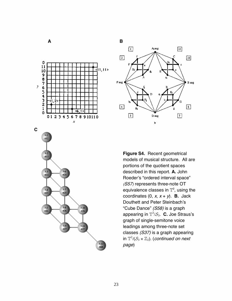
Figure S4. Recent geometrical models of musical structure. All are portions of the quotient spaces described in this report. A. John Roeder s “ordered interval space” (S57) represents three-note OT equivalence classes in T2, using the coordinates (0, x, x + y). B. Jack Douthett and Peter Steinbach s “Cube Dance” (S58) is a graph appearing in T3
/S3. C. Joe Straus s graph of single-semitone voice leadings among three-note set classes (S37) is a graph appearing in T2
/(S3 Z2). (continued on next page)
24
D E
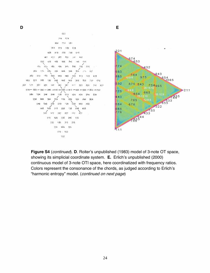
Figure S4 (continued). D. Roiter s unpublished (1983) model of 3-note OT space, showing its simplicial coordinate system. E. Erlich s unpublished (2000) continuous model of 3-note OTI space, here coordinatized with frequency ratios. Colors represent the consonance of the chords, as judged according to Erlich s “harmonic entropy” model. (continued on next page)
25
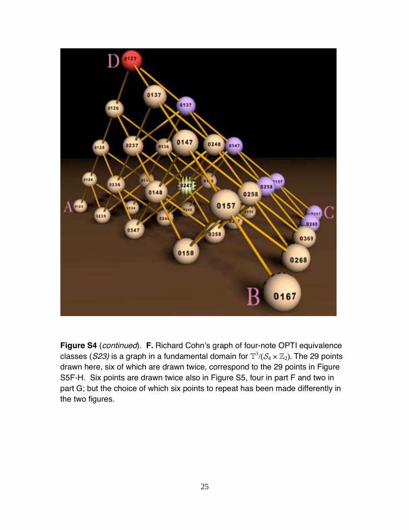
Figure S4 (continued). F. Richard Cohn s graph of four-note OPTI equivalence classes (S23) is a graph in a fundamental domain for T3
/(S4 Z2). The 29 points drawn here, six of which are drawn twice, correspond to the 29 points in Figure S5F-H. Six points are drawn twice also in Figure S5, four in part F and two in part G; but the choice of which six points to repeat has been made differently in the two figures.
26
0000
0011
0022
0033
0044
0055
0001
0012
0023
0034
0045
0056
0066
00e1
0002
0013
0024
0035
0046
0057
00e2
0003
0014
0025
0036
0047
00t2
00e3
0004
0015
0026
0037
0048
00t3
00e4
0005
0016
0027
0038
0093
00t4
00e5
0006
0017
0028
0039
0094
00t5
00e6
0007
0018
0029
0084
0095
00t6
00e7
0008
0019
002t
0085
0096
00t7
00e8
0009
001t
0075
0086
0097
00t8
00e9
000t
001e
0076
0087
0098
00t9
00et
000e
0066
0077
0088
0099
00tt
00ee
0000
0123
0134
0145
0156
0167
0124
0135
0146
0157
e124
0125
0136
0147
0158
e125
0126
0137
0148
t125
e126
0127
0138
0149
t126
e127
0128
0139
9126
t127
e128
0129
013t
9127
t128
e129
012t
8127
9128
t129
e12t
012e
0246
0257
0268
0247 0248
0258
e247
0248
0259
0249
t248
e249
024t0369
0123
0134
0145
0156
0167
0124
0135
0146
0157
0125
0136
0147
0158
0126
0137
0148
0127
0138
0149
0128
0139
0129
013t
012t012e
0246
0257
0268
0247
0258
0248
02590249
024t
0369
0000
0011
0022
0033
0044
0055
0001
0012
0023
0034
0045
00560066
0002
0013
0024
0035
0046
0057
0003
0014
0025
0036
0047
0004
0015
0026
0037
0048
0005
0016
0027
0038
0006
0017
0028
0039
0007
0018
0029
0008
0019
002t
0009
001t
000t
001e000e
0000
BA C D
E F G H
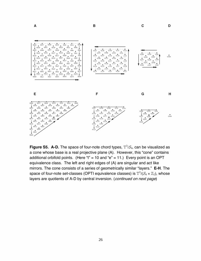
Figure S5. A-D. The space of four-note chord types, T3
/S4, can be visualized as a cone whose base is a real projective plane (A). However, this “cone” contains additional orbifold points. (Here “t” = 10 and “e” = 11.) Every point is an OPT equivalence class. The left and right edges of (A) are singular and act like mirrors. The cone consists of a series of geometrically similar “layers.” E-H. The space of four-note set-classes (OPTI equivalence classes) is T3
/(S4 Z2), whose layers are quotients of A-D by central inversion. (continued on next page)
27
0, c, 2c, 3c
0, c, 2c, 3c
0, c, 2c + x, 3c + x
0, c, 2c + x, 3c + x
0, c, 6, 6 + c
0, c, 6, 6+c
0, c, 6 – x, 6 + c + x
0, c, 2c, 3c
0, c, 2c, 3c
0, c, 2c + x, 3c + x
0, c, 6, 6 + c 0, c, 6 – x, 6 + c + x
0, c, 6 – x, 6 + c + x
0, c, 2c, 3c + x
0, c, 2c, 6 + c
0, c, 2c, 3c
0, c, 2c, 3c
0, c, 2c, 3c
0, c, 2c + x, 3c + x
0, c, 6, 6 + c0, c, 6 – x, 6 + c + x
0, c, 2c + y, 3c + y
0, c, 2c, 3c + x
0, c, 2c, 3c + x
I
K
J
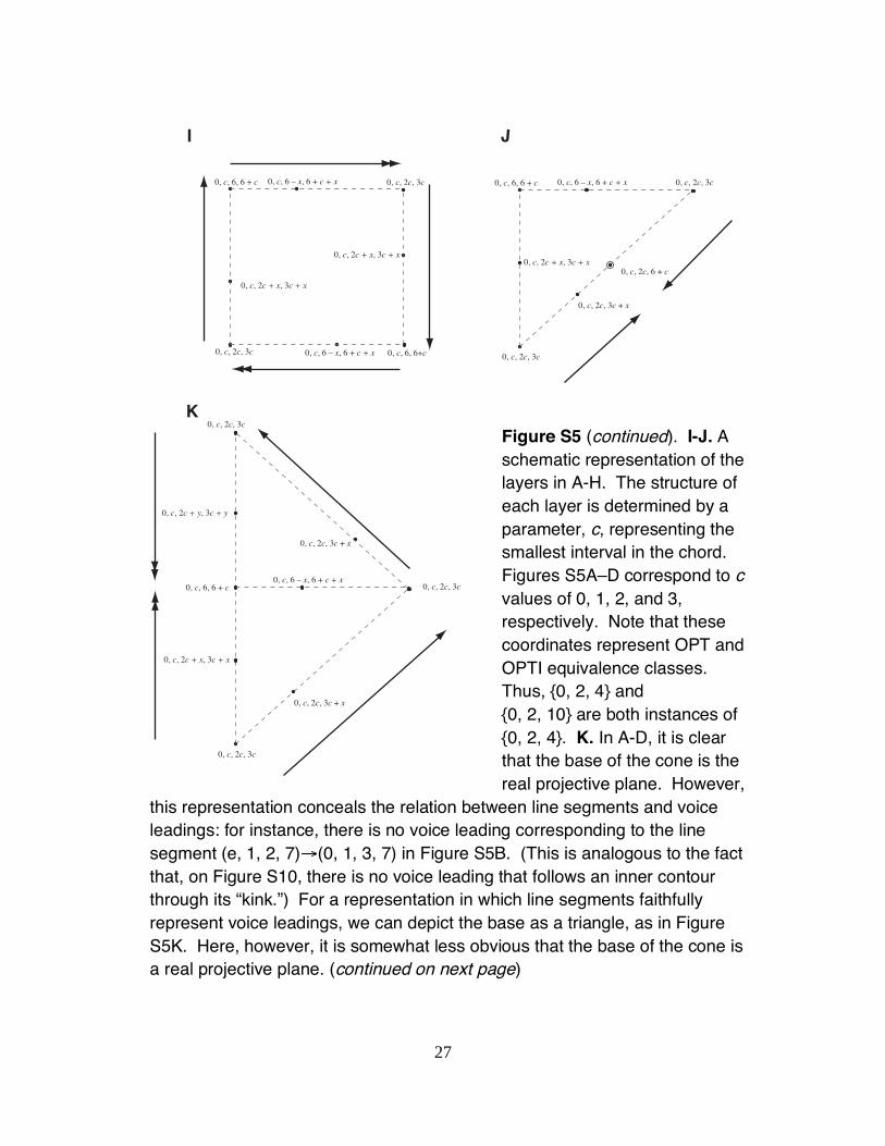
Figure S5 (continued). I-J. A schematic representation of the layers in A-H. The structure of each layer is determined by a parameter, c, representing the smallest interval in the chord. Figures S5A–D correspond to c values of 0, 1, 2, and 3, respectively. Note that these coordinates represent OPT and OPTI equivalence classes. Thus, {0, 2, 4} and {0, 2, 10} are both instances of {0, 2, 4}. K. In A-D, it is clear that the base of the cone is the real projective plane. However,
this representation conceals the relation between line segments and voice leadings: for instance, there is no voice leading corresponding to the line segment (e, 1, 2, 7) (0, 1, 3, 7) in Figure S5B. (This is analogous to the fact that, on Figure S10, there is no voice leading that follows an inner contour through its “kink.”) For a representation in which line segments faithfully represent voice leadings, we can depict the base as a triangle, as in Figure S5K. Here, however, it is somewhat less obvious that the base of the cone is a real projective plane. (continued on next page)
28
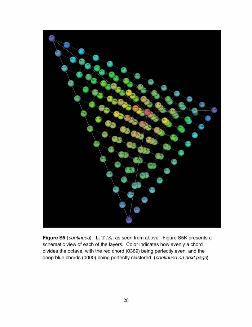
Figure S5 (continued). L. T3
/S4, as seen from above. Figure S5K presents a schematic view of each of the layers. Color indicates how evenly a chord divides the octave, with the red chord (0369) being perfectly even, and the deep blue chords (0000) being perfectly clustered. (continued on next page)
29
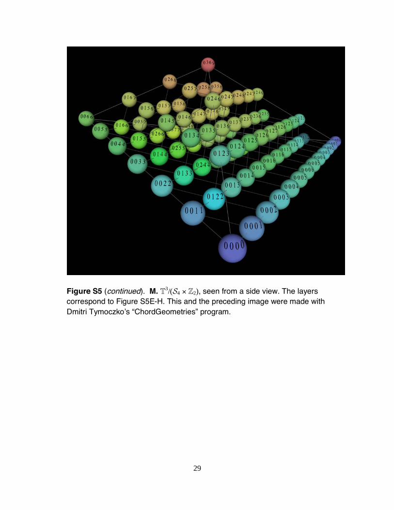
Figure S5 (continued). M. T3
/(S4 Z2), seen from a side view. The layers correspond to Figure S5E-H. This and the preceding image were made with Dmitri Tymoczko s “ChordGeometries” program.
30
CDf
CC
CD
CEf
CE
CF
CFs
GC
AfC
AC
BfC
BC
[CC]
CsCs
CsD
CsDs
CsE
DfF
DfGf
CsG
AfDf
ACs
BfDf
[BCs]
BCs
BD
BDs
BE
BF
FsB
GB
GsB
AB
AsB
BB
DD
DEf
DE
DF
DFs
DG
DAf
AD
[BfD]
BfD
BfEf
BfE
FBf
GfBf
GBf
AfBf
ABf
BfBf
EfEf
DsE
EfF
EfGf
EfG
EfAf
[EfA]AEf
EA
FA
FsA
GA
GsA
AA
EE
EF
EFs
EG
[EGs]
EGs
FAf
GfAf
GAf
AfAf
FF
FGf
[FG]
FG
FsG
GG
[FsFs]
FsFs
A
B
CA B
&?
œ œœ œ#
œ œ#œ œ
Figure S6. A–B. The progressions (D, E) (Ds, E) and (D, E) (E, Ds). C. The line segments in T2
/S2 corresponding to these progressions.
31
x
x
y
y
A
C
(a, b)
(–a, –b)
.
.
y
B
(a, b).
(a, b).
x
D
xy
(–a, 0) (a, 0)
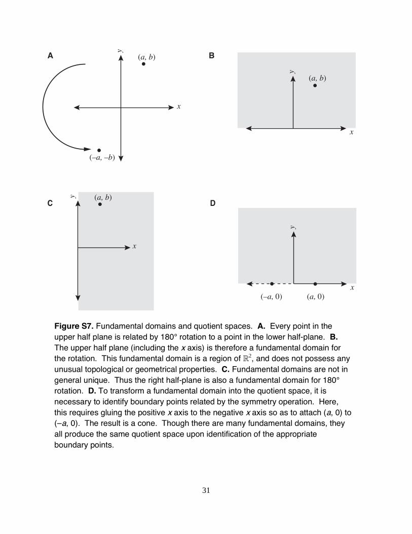
Figure S7. Fundamental domains and quotient spaces. A. Every point in the upper half plane is related by 180° rotation to a point in the lower half-plane. B. The upper half plane (including the x axis) is therefore a fundamental domain for the rotation. This fundamental domain is a region of R2, and does not possess any unusual topological or geometrical properties. C. Fundamental domains are not in general unique. Thus the right half-plane is also a fundamental domain for 180° rotation. D. To transform a fundamental domain into the quotient space, it is necessary to identify boundary points related by the symmetry operation. Here, this requires gluing the positive x axis to the negative x axis so as to attach (a, 0) to (–a, 0). The result is a cone. Though there are many fundamental domains, they all produce the same quotient space upon identification of the appropriate boundary points.
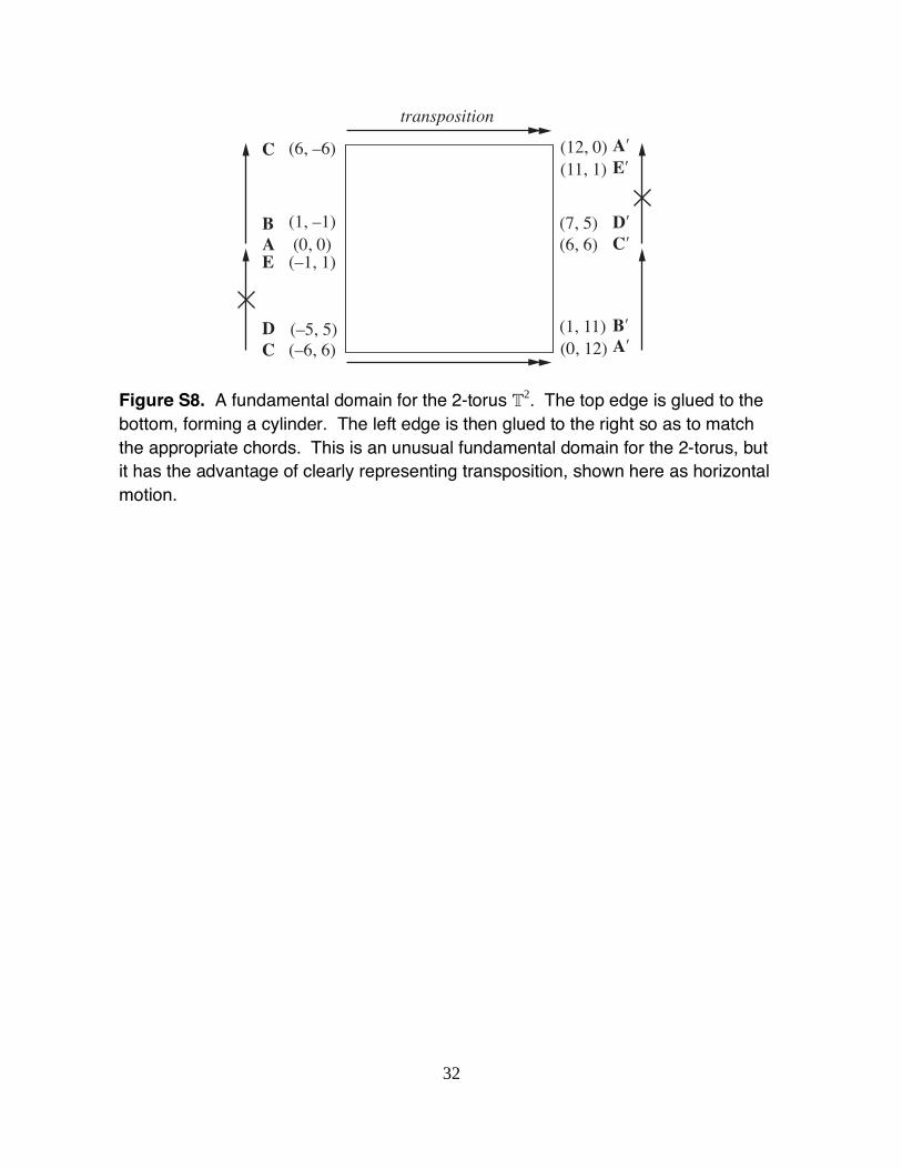
32
(0, 0)(1, –1)
(1, 11)
(12, 0)
(0, 12)
(6, –6)
(–6, 6)
(6, 6)(7, 5)
(–5, 5)
A(–1, 1)E
B
C
Aʹ
Aʹ(11, 1) Eʹ
Bʹ
Cʹ
CD
Dʹ
transposition
Figure S8. A fundamental domain for the 2-torus T2. The top edge is glued to the bottom, forming a cylinder. The left edge is then glued to the right so as to match the appropriate chords. This is an unusual fundamental domain for the 2-torus, but it has the advantage of clearly representing transposition, shown here as horizontal motion.
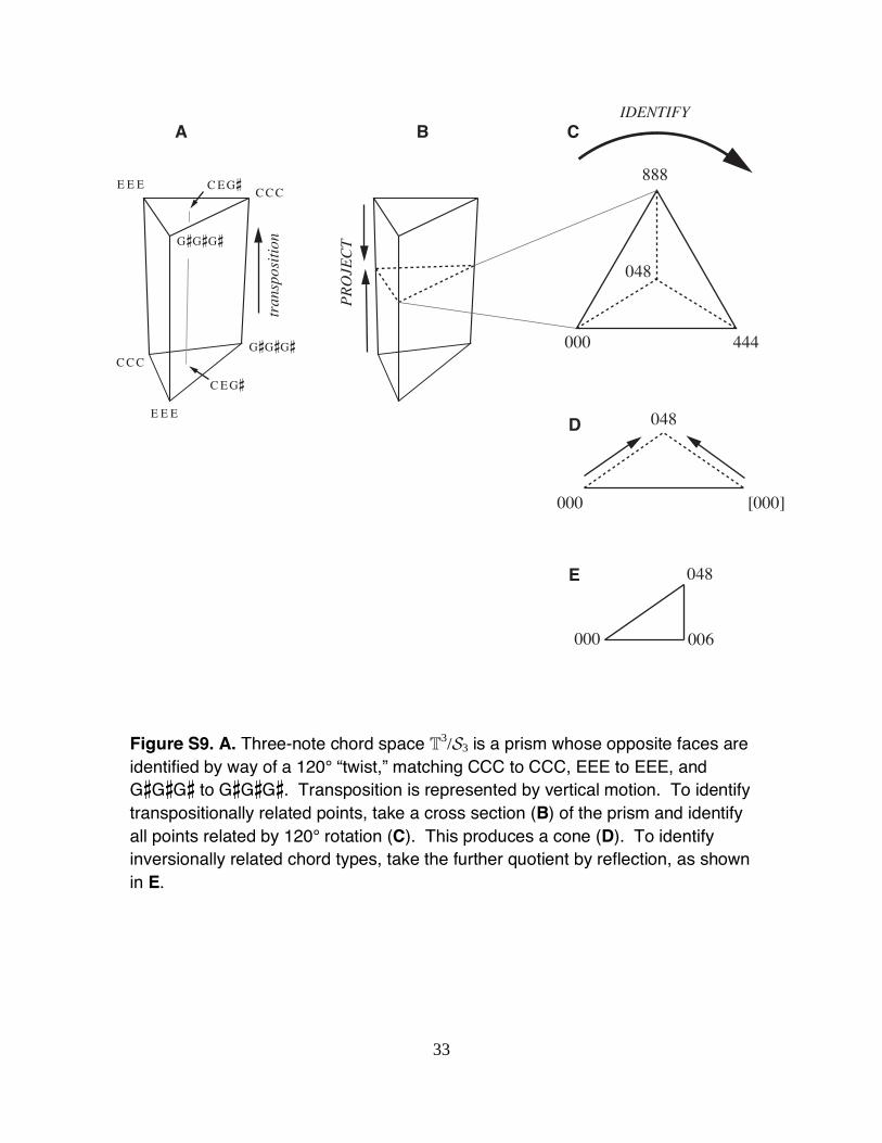
33
CCC
CCC
EEE
EEE
GsGsGs
CEGs
CEGs
GsGsGs
tran
spos
itio
n
PR
OJE
CT
IDENTIFY
000
000
006000
[000]
444
888
048
048
048
A B C
D
E
Figure S9. A. Three-note chord space T3
/S3 is a prism whose opposite faces are identified by way of a 120° “twist,” matching CCC to CCC, EEE to EEE, and GsGsGs to GsGsGs. Transposition is represented by vertical motion. To identify transpositionally related points, take a cross section (B) of the prism and identify all points related by 120° rotation (C). This produces a cone (D). To identify inversionally related chord types, take the further quotient by reflection, as shown in E.
34
Figure S10. Three-note OPT space (T2
/S3) can be understood as a series of similar “layers.” Here, the outermost layer contains chord-types whose smallest interval is 0; the next layer contains chord-types whose smallest interval is 1, and so on.
35
A D
E
B
C
&&
œ œœ œbœ œb
œ œb
œ œœ œbœ œb
œ œbœ œ
&&
œ œœ œbœ œb
œ œœ œ#œ œ
œ œœ œœ œ
1
2
3
(C4, E4, G4)
(Df4, Ef4, G4)
(Ef4, G4, Df4)
(G4, Df4, Ef4)
&&
œ œœ œbœ œb
œ œbœ œœ œb
œ œbœ œbœ œ
2
3
1
Squared unevenness:
Squared size:
–32 –
38 Squared spread: –
374 –
356
2 6 2
Squared size: 2 54 74T0 T–4 T–8
Figure S11. A. Beginning with a voice leading that does not touch the boundary of OPT space, transform the second chord by successively transposing its bottom note up by octave. B. Then consider the smallest voice leadings individually T-related to these. If one is using the Euclidean metric, the resulting voice leadings will connect chords summing to the same value, and their average squared size will be equal to the sum of the squared “unevenness” of the two original chords (here 10/3). (“Unevenness” is measured by the size of smallest voice leading from a chord to the nearest chord dividing the octave perfectly evenly.) C. In three-note OPT space, the three voice leadings in B represent three different line segments between the same two points, none touching the space s singular boundary. Their average squared length is equal to the sum of their endpoints squared distances to the cone s vertex. D. Beginning with any voice leading in pitch space, circularly permute the pitches of second chord. Consider the smallest voice leadings individually T-related to these. (In the example shown, these voice leadings are already as small as possible.) Using the Euclidean metric, the average squared size of these voice leadings (here 130/3) will be equal to the sum of the squared “spread” of the two original chords. (“Spread” is measured by the size of smallest voice leading from the original chord to the nearest chord with just a single pitch class.) E. The three voice leadings in D, shown in T-space.
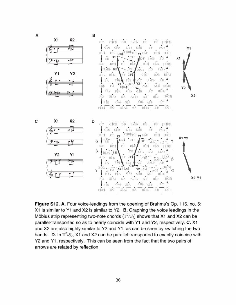
36
X1
Y1
Y1
X2
Y2
X1
X2
Y2
&?
œ œ œ œ#œ œ# œ œ#
&?
œ œ œ œœ# œ# œ# œ
&?
œ œ œ œ#œ œ# œ œ#
?
&
œ# œ œ# œ#œ œ œ œ
X1 X2A
C
B
D
Y1 Y2
X1 X2
Y2 Y1
CDf
CC
CD CDs
CE
CF
CFs
GC
AfC
AC
BfC
BC
[CC]
CsCs
CsD
CsDs
CsE
DfF
DfGf
CsG
AfDf
ACs
BfDf
[BCs]
BCs
BD
BDs
BE
BF
FsBGB
GsB
AB
AsB
BB
DD
DEf
DE
DF
DFs
DG
DAf
AD
[BfD]
BfD
BfEf
BfE
FBf
FsAs
GBf
AfBf
ABf
BfBf
EfEf
DsE
EfF
EfGf
EfG
EfAf
[EfA]AEf
EA
FA
FsA
GA
GsA
AA
EE
EF
EFs
EG
[EGs]
EGs
FAf
GfAf
GAf
AfAf
FF
FGf
[FG]
FG
FsG
GG
[FsFs]
FsFs
X1Y1
X2 Y2
CDf
CC
CD
CDs
CE
CF
CFs
GC
AfC
AC
BfC
BC
[CC]
CsCs
CsD
CsDs
CsE
DfF
DfGf
CsG
AfDf
ACsBfDf
[BCs]
BCs
BD
BDs
BE
BF
FsBGB
GsB
AB
AsB
BB
DD
DEf
DE
DF
DFs
DG
DAfAD
[BfD]
BfD
BfEf
BfE
FBf
FsAs
GBf
AfBf
ABf
BfBf
EfEf
DsE
EfF
EfGf
EfG
EfAf
[EfA]AEf
EA
FAFsA
GA
GsA
AA
EE
EF
EFs
EG[EGs]
EGs
FAf
GfAf
GAf
AfAf
FF
FGf
[FG]
FG
FsG
GG
[FsFs]
FsFs
X1 Y1
X2 Y2
α
β
γ
γ
β
α
Figure S12. A. Four voice-leadings from the opening of Brahms s Op. 116, no. 5: X1 is similar to Y1 and X2 is similar to Y2. B. Graphing the voice leadings in the Möbius strip representing two-note chords (T2
/S2) shows that X1 and X2 can be parallel-transported so as to nearly coincide with Y1 and Y2, respectively. C. X1 and X2 are also highly similar to Y2 and Y1, as can be seen by switching the two hands. D. In T2
/S2, X1 and X2 can be parallel transported to exactly coincide with Y2 and Y1, respectively. This can be seen from the fact that the two pairs of arrows are related by reflection.
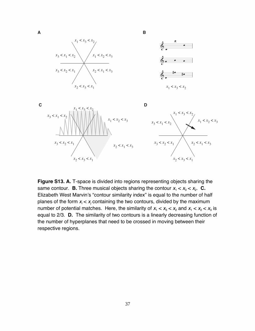
37
x1 < x2 < x3
x2 < x1 < x3
x3 < x1 < x2
x3 < x2 < x1
x1 < x3 < x2
x1 < x3 < x2x2 < x3 < x1
x1 < x2 < x3
x2 < x1 < x3
x3 < x1 < x2
x3 < x2 < x1
x1 < x3 < x2
x2 < x3 < x1
x1 < x2 < x3
x2 < x1 < x3
x3 < x1 < x2
x3 < x2 < x1
x1 < x3 < x2
x2 < x3 < x1
& œœ œ
& œ œ œ
& œ œ# œ#
A B
C D
Figure S13. A. T-space is divided into regions representing objects sharing the same contour. B. Three musical objects sharing the contour x1 < x3 < x2. C. Elizabeth West Marvin s “contour similarity index” is equal to the number of half planes of the form xi < xj containing the two contours, divided by the maximum number of potential matches. Here, the similarity of x1 < x3 < x2 and x1 < x2 < x3 is equal to 2/3. D. The similarity of two contours is a linearly decreasing function of the number of hyperplanes that need to be crossed in moving between their respective regions.
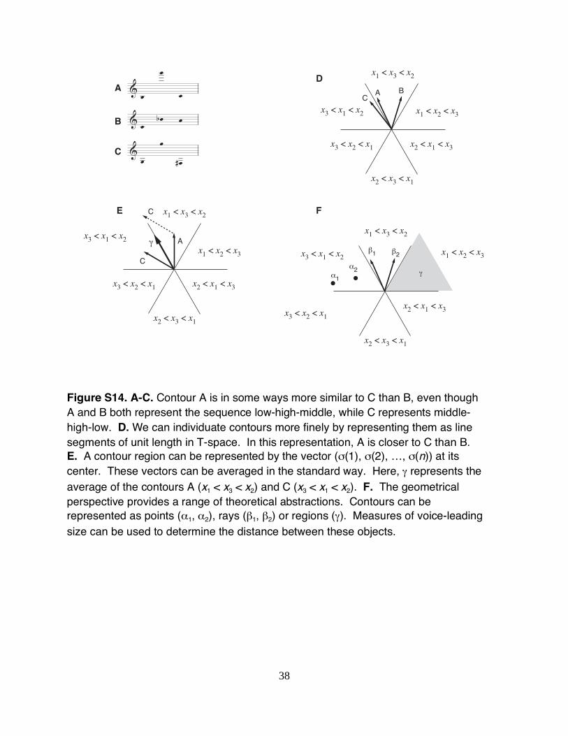
38
x1 < x2 < x3
x2 < x1 < x3
x3 < x1 < x2
x3 < x2 < x1
x1 < x3 < x2
x2 < x3 < x1
A AC
B
B
C
D
FE
& œœ
œ& œ œb œ
& œœ
œ#
x1 < x2 < x3
x2 < x1 < x3
x3 < x1 < x2
x3 < x2 < x1
x1 < x3 < x2
x2 < x3 < x1
β1
γα2
α1
β2x1 < x2 < x3
x2 < x1 < x3
x3 < x1 < x2
x3 < x2 < x1
x1 < x3 < x2
x2 < x3 < x1
A
C
C
γ
Figure S14. A-C. Contour A is in some ways more similar to C than B, even though A and B both represent the sequence low-high-middle, while C represents middle-high-low. D. We can individuate contours more finely by representing them as line segments of unit length in T-space. In this representation, A is closer to C than B. E. A contour region can be represented by the vector ( (1), (2), …, (n)) at its center. These vectors can be averaged in the standard way. Here, represents the average of the contours A (x1 < x3 < x2) and C (x3 < x1 < x2). F. The geometrical perspective provides a range of theoretical abstractions. Contours can be represented as points ( 1, 2), rays ( 1, 2) or regions ( ). Measures of voice-leading size can be used to determine the distance between these objects.
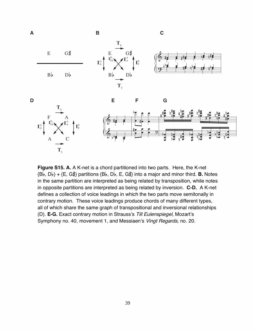
39
E Gs
Bf Df
E Gs
Bf Df
T4
II
I
T3
F A
A C
T4
T3
A
ED F G
B C
&?
œ# œ œ# œ œ œ#œ œ œ# œ œb œnœb œ œ œb œ œbœb œ œ# œn œ# œn
&&
œ# œœ œœb œœb œ
œœb œ
œ#œœ
œœ# œœ œœ ?
œœœ## œœœn#n œœœ#n# œœœ## œœœn#n œœœ## œœœn#n œœœ#n#
œœœb œœœbn œœœ#n œœœb œœœbnn œœœb œœœbnb œœœnn
GG
IAA E
F
DEf
II
IGG
IAA E
F
DEf
Figure S15. A. A K-net is a chord partitioned into two parts. Here, the K-net {Bf, Df} + {E, Gs} partitions {Bf, Df, E, Gs} into a major and minor third. B. Notes in the same partition are interpreted as being related by transposition, while notes in opposite partitions are interpreted as being related by inversion. C-D. A K-net defines a collection of voice leadings in which the two parts move semitonally in contrary motion. These voice leadings produce chords of many different types, all of which share the same graph of transpositional and inversional relationships (D). E-G. Exact contrary motion in Strauss s Till Eulenspiegel, Mozart s Symphony no. 40, movement 1, and Messiaen s Vingt Regards, no. 20.
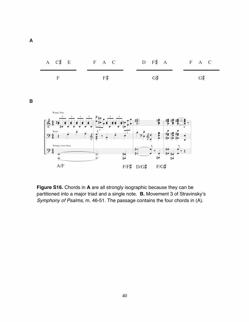
40
A Cs E
F
A
B
D Fs A
Gs
F A C
Gs
F A C
Fs
&??
44
44
44
3œœ# œ# œœ3
œ œœ œ3œœ œ œœ
3
œ œœ œŒ œ> œ> œ> &
ww>
3
œœ> œœ## œœ3œœ œ œœ
3œœ œ œœ3
œœnnœœ œœ
jœœœ> ‰ œ> œ> œ>
..˙ œœ##
....˙# œœœœnœ> œœ> œœ>
œœœœ? &
˙##jœœ ‰ œœ#
œœœœ# œœœœn œœœœ#Jœœœœ ‰
œœœœ## œœœœnnœœœœ## œœ
œœ## œœ##jœœ ‰ Œ
Winds, Pno.
Brass
Strings, Low brass
A/F D/Gs F/GsF/Fs
Figure S16. Chords in A are all strongly isographic because they can be partitioned into a major triad and a single note. B. Movement 3 of Stravinsky s Symphony of Psalms, m. 46-51. The passage contains the four chords in (A).
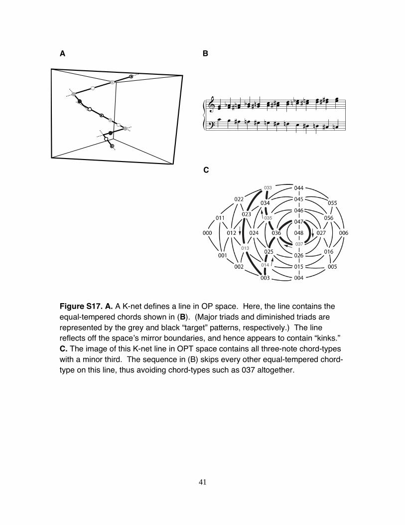
41
A B
&
?
œœ
œœ
b œœ
n#
œœ
b œœ
n#
œœ
œœ
##
œœ
œœ
bn
œœ
n#
œœ
œœ
##
œœ
œ œ œ# œn œ# œn œ# œn œ œ# œn œ# œn
C
037
035
033
013
014
Figure S17. A. A K-net defines a line in OP space. Here, the line contains the equal-tempered chords shown in (B). (Major triads and diminished triads are represented by the grey and black “target” patterns, respectively.) The line reflects off the space s mirror boundaries, and hence appears to contain “kinks.” C. The image of this K-net line in OPT space contains all three-note chord-types with a minor third. The sequence in (B) skips every other equal-tempered chord-type on this line, thus avoiding chord-types such as 037 altogether.
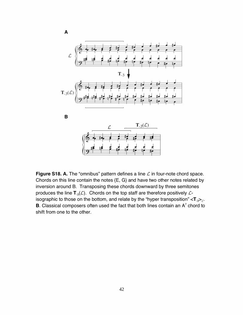
42
A
&?
œ œ# œ œ œ# œ œ# œ œ œ# œ œ#œ œ œ œ œ œ œ œ œ œ œ œœ œ œ œ œ œ œ œ œ œ œ œœ# œn œ œ# œn œ# œn œ# œn œ œ# œn
&?
œ# œ œ# œ œ# œ œ œ# œ œ# œ œœ œ œ œ œ œ œ œ œ œ œ œœ# œ# œ# œ# œ# œ# œ# œ# œ# œ# œ# œ#œ# œn œ# œn œ# œn œ œ# œn œ# œn œ
L
T-3
T-3
(L)
B
&
?
œ œ# œ œ œ# œ œ œ
œ œ œ œ œ œ# œ œ#
œ œ œ œ œ œ œ œœ# œn œ œ# œn œ# œn œ#
L T-3(L)
Figure S18. A. The “omnibus” pattern defines a line L in four-note chord space. Chords on this line contain the notes {E, G} and have two other notes related by inversion around B. Transposing these chords downward by three semitones produces the line T-3(L). Chords on the top staff are therefore positively L-isographic to those on the bottom, and relate by the “hyper transposition” <T-3>L. B. Classical composers often used the fact that both lines contain an A7 chord to shift from one to the other.
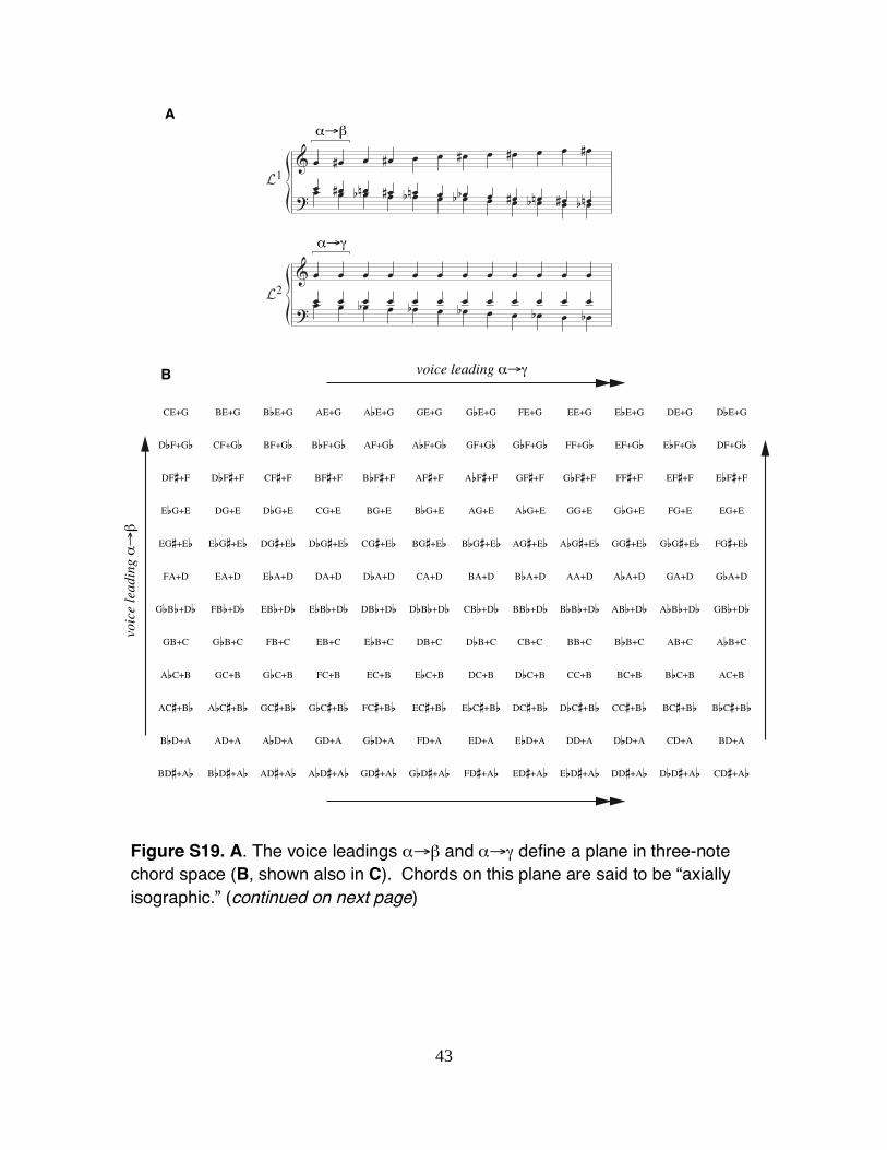
43
A
CE+G BE+G BfE+G AE+G AfE+G GE+G GfE+G FE+G EE+G EfE+G DE+G DfE+G
DfF+Gf CF+Gf BF+Gf BfF+Gf AF+Gf AfF+Gf GF+Gf GfF+Gf FF+Gf EF+Gf EfF+Gf DF+Gf
DFs+F DfFs+F CFs+F BFs+F BfFs+F AFs+F AfFs+F GFs+F GfFs+F FFs+F EFs+F EfFs+F
EfG+E DG+E DfG+E CG+E BG+E BfG+E AG+E AfG+E GG+E GfG+E FG+E EG+E
EGs+Ef EfGs+Ef DGs+Ef DfGs+Ef CGs+Ef BGs+Ef BfGs+Ef AGs+Ef AfGs+Ef GGs+Ef GfGs+Ef FGs+Ef
FA+D EA+D EfA+D DA+D DfA+D CA+D BA+D BfA+D AA+D AfA+D GA+D GfA+D
GfBf+Df FBf+Df EBf+Df EfBf+Df DBf+Df DfBf+Df CBf+Df BBf+Df BfBf+Df ABf+Df AfBf+Df GBf+Df
GB+C GfB+C FB+C EB+C EfB+C DB+C DfB+C CB+C BB+C BfB+C AB+C AfB+C
AfC+B GC+B GfC+B FC+B EC+B EfC+B DC+B DfC+B CC+B BC+B BfC+B AC+B
ACs+Bf AfCs+Bf GCs+Bf GfCs+Bf FCs+Bf ECs+Bf EfCs+Bf DCs+Bf DfCs+Bf CCs+Bf BCs+Bf BfCs+Bf
BfD+A AD+A AfD+A GD+A GfD+A FD+A ED+A EfD+A DD+A DfD+A CD+A BD+A
BDs+Af BfDs+Af ADs+Af AfDs+Af GDs+Af GfDs+Af FDs+Af EDs+Af EfDs+Af DDs+Af DfDs+Af CDs+Af
&?
œ œ# œ œ# œ œ œ# œ œ# œ œ œ#œ œ# œn œ# œn œ œb œ œ# œn œ# œnœ œ œb œ œb œ œb œ œ œb œ œb
&?
œ œ œ œ œ œ œ œ œ œ œ œœ œ œ œ œ œ œ œ œ œ œ œœ œ œb œ œb œ œb œ œ œb œ œb
L1
L2
B
α→β
α→γ
voice leading α→γ
voic
e le
adin
g α→β
Figure S19. A. The voice leadings and define a plane in three-note chord space (B, shown also in C). Chords on this plane are said to be “axially isographic.” (continued on next page)
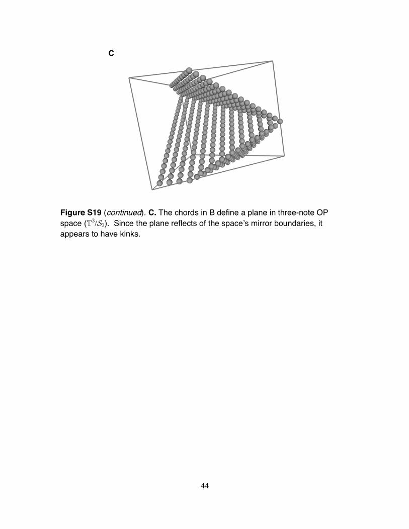
44
C
Figure S19 (continued). C. The chords in B define a plane in three-note OP space (T3
/S3). Since the plane reflects of the space s mirror boundaries, it appears to have kinks.
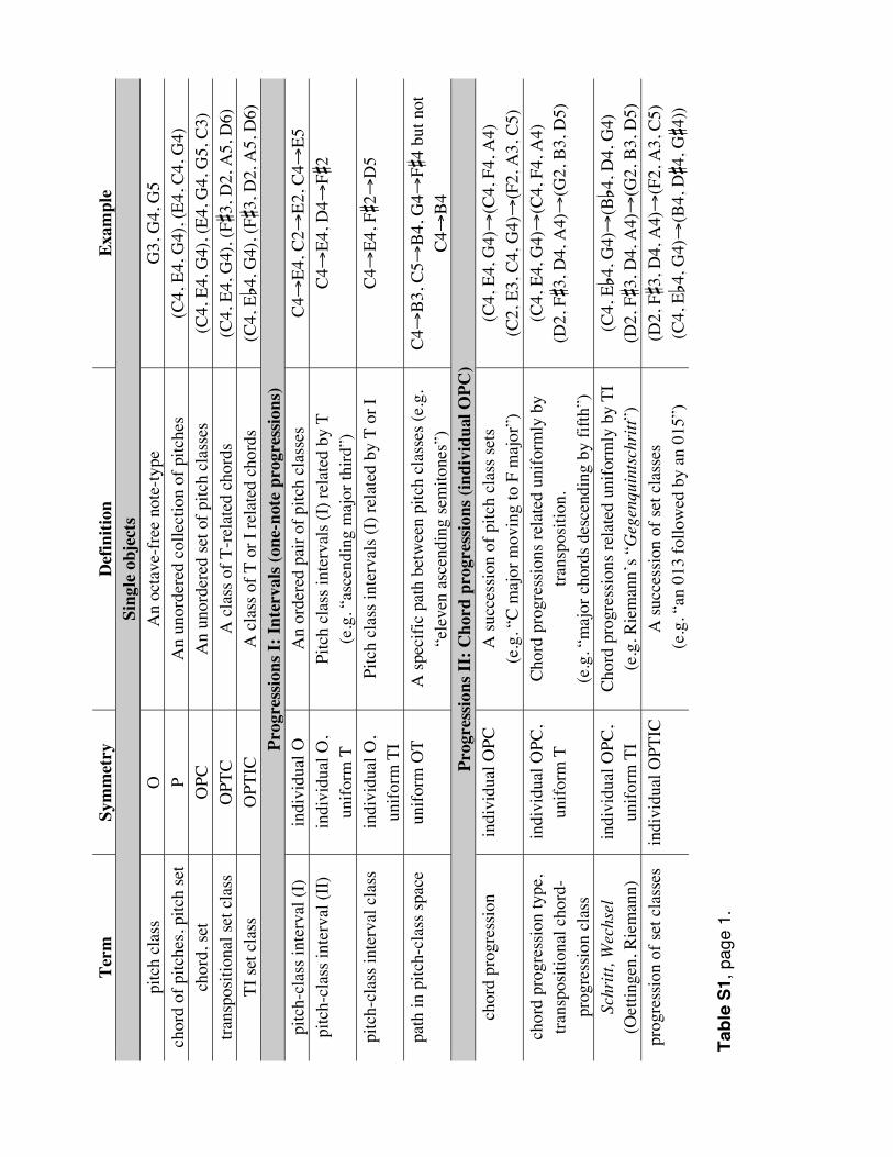
Tab
le S
1, p
age
1.
Ter
m
Sym
met
ry
Def
init
ion
Exa
mpl
e Si
ngle
obj
ects
pi
tch
clas
s O
A
n oc
tave
-fre
e no
te-t
ype
G3,
G4,
G5
chor
d of
pitc
hes,
pitc
h se
t P
An
unor
dere
d co
llect
ion
of p
itche
s (C
4, E
4, G
4), (
E4,
C4,
G4)
ch
ord,
set
O
PC
An
unor
dere
d se
t of
pitc
h cl
asse
s (C
4, E
4, G
4), (
E4,
G4,
G5,
C3)
tr
ansp
ositi
onal
set
cla
ss
OPT
C
A c
lass
of
T-r
elat
ed c
hord
s (C
4, E
4, G
4), (
Fs3,
D2,
A5,
D6)
T
I se
t cla
ss
OPT
IC
A c
lass
of
T o
r I
rela
ted
chor
ds
(C4,
Ef4
, G4)
, (Fs3
, D2,
A5,
D6)
P
rogr
essi
ons
I: I
nter
vals
(on
e-no
te p
rogr
essi
ons)
pi
tch-
clas
s in
terv
al (
I)
indi
vidu
al O
A
n or
dere
d pa
ir o
f pi
tch
clas
ses
C4
E4,
C2
E2,
C4
E5
pitc
h-cl
ass
inte
rval
(II
) in
divi
dual
O,
unif
orm
T
Pit
ch c
lass
inte
rval
s (I
) re
late
d by
T
(e.g
. “as
cend
ing
maj
or th
ird”
) C
4E
4, D
4Fs2
pitc
h-cl
ass
inte
rval
cla
ss
indi
vidu
al O
, un
ifor
m T
I P
itch
cla
ss in
terv
als
(I)
rela
ted
by T
or
I C
4E
4, Fs2
D5
path
in p
itch
-cla
ss s
pace
un
ifor
m O
T
A s
peci
fic
path
bet
wee
n pi
tch
clas
ses
(e.g
. “e
leve
n as
cend
ing
sem
itone
s”)
C4
B3,
C5
B4,
G4
Fs4
but
not
C
4B
4 P
rogr
essi
ons
II:
Cho
rd p
rogr
essi
ons
(ind
ivid
ual O
PC
) ch
ord
prog
ress
ion
indi
vidu
al O
PC
A
suc
cess
ion
of p
itch
cla
ss s
ets
(e.g
. “C
maj
or m
ovin
g to
F m
ajor
”)
(C4,
E4,
G4)
(C4,
F4,
A4)
(C2,
E3,
C4,
G4)
(F2,
A3,
C5)
ch
ord
prog
ress
ion
type
, tr
ansp
ositi
onal
cho
rd-
prog
ress
ion
clas
s
indi
vidu
al O
PC,
unif
orm
T
Cho
rd p
rogr
essi
ons
rela
ted
unif
orm
ly b
y tr
ansp
ositi
on.
(e.g
. “m
ajor
cho
rds
desc
endi
ng b
y fi
fth”
)
(C4,
E4,
G4)
(C4,
F4,
A4)
(D
2, Fs3
, D4,
A4)
(G2,
B3,
D5)
Schr
itt,
Wec
hsel
(O
ettin
gen,
Rie
man
n)
indi
vidu
al O
PC,
unif
orm
TI
Cho
rd p
rogr
essi
ons
rela
ted
unif
orm
ly b
y T
I (e
.g. R
iem
ann’
s “G
egen
quin
tsch
ritt
”)
(C4,
Ef4
, G4)
(Bf4
, D4,
G4)
(D
2, Fs3
, D4,
A4)
(G2,
B3,
D5)
pr
ogre
ssio
n of
set
cla
sses
in
divi
dual
OP
TIC
A
suc
cess
ion
of s
et c
lass
es
(e.g
. “an
013
fol
low
ed b
y an
015
”)
(D2,
Fs3
, D4,
A4)
(F2,
A3,
C5)
(C
4, Ef4
, G4)
(B4,
Ds4
, Gs4
))
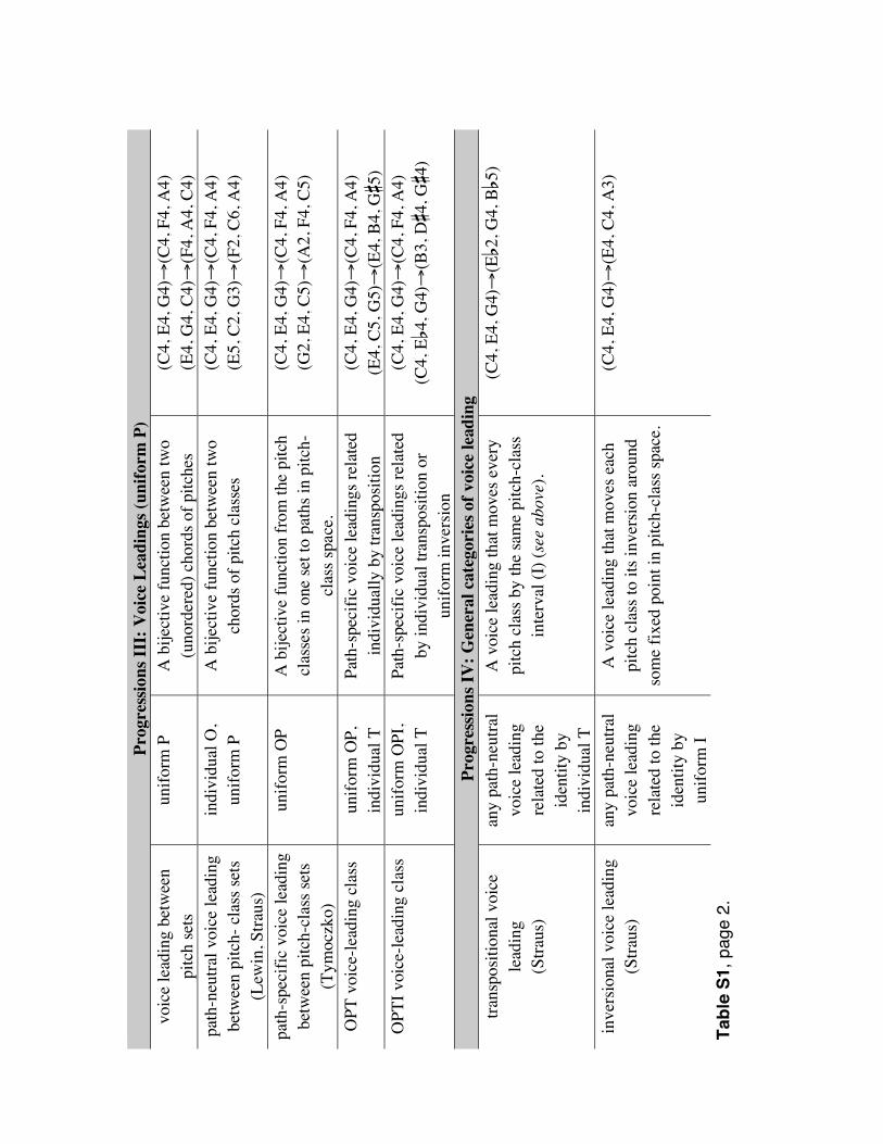
P
rogr
essi
ons
III:
Voi
ce L
eadi
ngs
(uni
form
P)
voic
e le
adin
g be
twee
n pi
tch
sets
un
ifor
m P
A
bij
ecti
ve f
unct
ion
betw
een
two
(uno
rder
ed)
chor
ds o
f pi
tche
s (C
4, E
4, G
4)(C
4, F
4, A
4)
(E4,
G4,
C4)
(F4,
A4,
C4)
pa
th-n
eutr
al v
oice
lead
ing
betw
een
pitc
h- c
lass
set
s (L
ewin
, Str
aus)
indi
vidu
al O
, un
ifor
m P
A
bije
ctiv
e fu
nctio
n be
twee
n tw
o ch
ords
of
pitc
h cl
asse
s (C
4, E
4, G
4)(C
4, F
4, A
4)
(E5,
C2,
G3)
(F2,
C6,
A4)
path
-spe
cifi
c vo
ice
lead
ing
betw
een
pitc
h-cl
ass
sets
(T
ymoc
zko)
unif
orm
OP
A
bij
ecti
ve f
unct
ion
from
the
pitc
h cl
asse
s in
one
set
to p
aths
in p
itch-
clas
s sp
ace.
(C4,
E4,
G4)
(C4,
F4,
A4)
(G
2, E
4, C
5)(A
2, F
4, C
5)
OP
T v
oice
-lea
ding
cla
ss
unif
orm
OP
, in
divi
dual
T
Pat
h-sp
ecif
ic v
oice
lead
ings
rel
ated
in
divi
dual
ly b
y tr
ansp
ositi
on
(C4,
E4,
G4)
(C4,
F4,
A4)
(E
4, C
5, G
5)(E
4, B
4, Gs5
) O
PT
I vo
ice-
lead
ing
clas
s un
ifor
m O
PI,
in
divi
dual
T
Pat
h-sp
ecif
ic v
oice
lead
ings
rel
ated
by
indi
vidu
al tr
ansp
ositi
on o
r un
ifor
m in
vers
ion
(C4,
E4,
G4)
(C4,
F4,
A4)
(C
4, Ef4
, G4)
(B3,
Ds4
, Gs4
)
Pro
gres
sion
s IV
: G
ener
al c
ateg
orie
s of
voi
ce le
adin
g tr
ansp
ositi
onal
voi
ce
lead
ing
(Str
aus)
any
path
-neu
tral
vo
ice
lead
ing
rela
ted
to th
e id
entit
y by
in
divi
dual
T
A v
oice
lead
ing
that
mov
es e
very
pi
tch
clas
s by
the
sam
e pi
tch-
clas
s in
terv
al (
I) (
see
abov
e).
(C4,
E4,
G4)
(Ef2
, G4,
Bf5
)
inve
rsio
nal v
oice
lead
ing
(Str
aus)
an
y pa
th-n
eutr
al
voic
e le
adin
g re
late
d to
the
iden
tity
by
unif
orm
I
A v
oice
lead
ing
that
mov
es e
ach
pitc
h cl
ass
to it
s in
vers
ion
arou
nd
som
e fi
xed
poin
t in
pitc
h-cl
ass
spac
e.
(C4,
E4,
G4)
(E4,
C4,
A3)
Tab
le S
1, p
age
2.
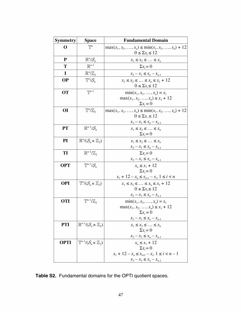
47
Symmetry Space Fundamental Domain
O Tn max(x1, x2, …, xn) min(x1, x2, …, xn) + 12
0 xi 12
P Rn/Sn x1 x2 … xn
T Rn-1 xi = 0
I Rn/Z2 x2 – x1 xn – xn-1
OP Tn/Sn x1 x2 … xn x1 + 12
0 xi 12
OT Tn-1 min(x1, x2, …, xn) = x1
max(x1, x2, …, xn) x1 + 12 xi = 0
OI Tn/Z2 max(x1, x2, …, xn) min(x1, x2, …, xn) + 12
0 xi 12 x2 – x1 xn – xn-1
PT Rn-1/Sn x1 x2 … xn
xi = 0
PI Rn/(Sn Z2) x1 x2 … xn
x2 – x1 xn – xn-1
TI Rn-1/Z2 xi = 0
x2 – x1 xn – xn-1
OPT Tn-1/Sn xn x1 + 12
xi = 0 x1 + 12 – xn xi+1 – xi, 1 i < n
OPI Tn/(Sn Z2) x1 x2 … xn x1 + 12
0 xi 12 x2 – x1 xn – xn-1
OTI Tn-1/Z2 min(x1, x2, …, xn) = x1
max(x1, x2, …, xn) x1 + 12 xi = 0
x2 – x1 xn – xn-1
PTI Rn-1/(Sn Z2) x1 x2 … xn
xi = 0 x2 – x1 xn – xn-1
OPTI Tn-1/(Sn Z2) xn x1 + 12
xi = 0 x1 + 12 – xn xi+1 – xi, 1 i < n – 1
x2 – x1 xn – xn-1
Table S2. Fundamental domains for the OPTI quotient spaces.
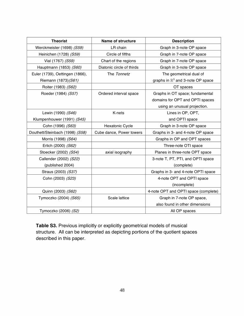
48
Theorist Name of structure Description
Werckmeister (1698) (S59) LR chain Graph in 3-note OP space
Heinichen (1728) (S59) Circle of fifths Graph in 7-note OP space
Vial (1767) (S59) Chart of the regions Graph in 7-note OP space
Hauptmann (1853) (S60) Diatonic circle of thirds Graph in 3-note OP space
Euler (1739), Oettingen (1866),
Riemann (1873)(S61)
The Tonnetz The geometrical dual of
graphs in R3 and 3-note OP space
Roiter (1983) (S62) OT spaces
Roeder (1984) (S57) Ordered interval space Graphs in OT space; fundamental
domains for OPT and OPTI spaces
using an unusual projection.
Lewin (1990) (S46)
Klumpenhouwer (1991) (S45)
K-nets Lines in OP, OPT,
and OPTI space
Cohn (1996) (S63) Hexatonic Cycle Graph in 3-note OP space
Douthett/Steinbach (1998) (S58) Cube dance, Power towers Graphs in 3- and 4-note OP space
Morris (1998) (S64) Graphs in OP and OPT spaces
Erlich (2000) (S62) Three-note OTI space
Stoecker (2002) (S54) axial isography Planes in three-note OPT space
Callender (2002) (S22)
(published 2004)
3-note T, PT, PTI, and OPTI space
(complete)
Straus (2003) (S37) Graphs in 3- and 4-note OPTI space
Cohn (2003) (S23) 4-note OPT and OPTI space
(incomplete)
Quinn (2003) (S62) 4-note OPT and OPTI space (complete)
Tymoczko (2004) (S65) Scale lattice Graph in 7-note OP space,
also found in other dimensions
Tymoczko (2006) (S2) All OP spaces
Table S3. Previous implicitly or explicitly geometrical models of musical structure. All can be interpreted as depicting portions of the quotient spaces described in this paper.
49
REFERENCES AND NOTES
S1. This equivalence class consists of all three-voice progressions that either move the
root, third, and fifth of major triad by x, x + 1, and x + 2 semitones, respectively, or the
root, third, and fifth of a minor triad by x – 2, x – 1, and x semitones, respectively, where
x is any real number.
S2. D. Tymoczko, Science 313, 72 (2006).
S3. This definition of “chord type” is a technical term of art that corresponds reasonably
well with ordinary usage. In some circumstances, however, musicians use “chord type”
to refer to other equivalence classes—such as PT equivalence classes.
S4. J. P. Rameau, Treatise on Harmony (Dover, New York, 1971).
S5. See H. Klumpenhouwer, Music Theory Online 0.9 (1994).
S6. D. Lewin, Generalized Musical Intervals and Transformations (Yale, New Haven,
1987).
S7. G. Mazzola, The Topos of Music (Birkhäuser, Boston, 2002).
S8. If one were to follow Allen Forte in identifying homometric or Z-related points,
such as (C, Cs, E, Fs)OPTI and (C, Cs, Ds, G)OPTI in four-note OPTI space (T3/[S4 Z2]),
there would not be a well-defined coordinate system at the point of identification. Thus,
quotient spaces formed using this equivalence relation will be significantly less
straightforward than those considered in this paper: in particular, distance cannot be
interpreted as representing voice leading. For more on these spaces, see reference 9.
S9. I. Quinn, Perspectives of New Music 44.2, 114 (2006).
S10. Perceptual models of voice-leading distance need to be quite complex, as there are
subtle interactions between displacement size and the number of moving voices, the
direction of motion, and so on. See reference 11.
S11. C. Callender, and N. Rogers, Proceedings of the International Conference of Music Perception and Cognition 9, 1686 (2006). S12. A. Bregman, Auditory Scene Analysis (Cambridge, MIT Press, 1990). S13. D. Huron, Music Perception 19, 1 (2001). S14. C. Masson, Nouveau Traité des Règles pour la Composition de la Musique (Da
Capo, New York, 1967).
S15. O. Hostinsky, Die Lehre von den musikalischen Klängen (H. Dominicus, Prague,
1879).
S16. A. Schoenberg, Theory of Harmony (University of California, Los Angeles, 1983).
S17. Note that the distribution constraint is a weakened version of the triangle inequality:
it asserts that all voice leadings such as B in Figure S6C, which form two legs of a
triangle by “bouncing off” a singularity, must be at least as large as the voice leading
forming the third leg of the triangle (e.g. A in the same figure). However, not all
50
triangles can be translated so that they are of this form. Consequently, the distribution
constraint is consistent with, but does not imply, the triangle inequality.
S18. The C operation is an isometry of the L norm. Hence, if one is willing to use this
metric, then distance in C spaces can be taken to represent voice-leading size.
S19. The claim that A B is significantly larger than C4 G4 depends on the stipulation that the motion from A to B consists of a number of conceptually distinct voices. In many cases (for instance, a string section playing in unison), such slight variations in pitch would not be conceived (or perceived) as distinct, and should instead be represented as a single, fused voice moving from C4 to G4. S20. A. Hatcher, Algebraic Topology (Cambridge, New York, 2002). S21. W. Thurston, The Geometry and Topology of Three Manifolds, available at
http://www.msri.org/publications/books/gt3m/.
S22. C. Callender, Music Theory Online 10.3 (2004).
S23. R. Cohn, Music Theory Online 9.4 (2003).
S24. http://music.princeton.edu/~dmitri/ChordGeometries.html
S25. R. Hall and D. Tymoczko, paper presented to the tenth annual Bridges Conference,
Donostia, Spain, July 24-27, 2007.
S26. R. Morris, Perspectives of New Music 18, 445 (1979-80).
S27. C. Lord, Journal of Music Theory 25, 91 (1981).
S28. E. Isaacson, Journal of Music Theory 34, 1 (1990). S29. D. Scott, and E. Isaacson, Perspectives of New Music 36.2, 107 (1998). S30. J. Rahn, Perspectives of New Music 18, 483 (1979-80).
S31. D. Lewin, Perspectives of New Music 18, 498 (1979-80).
S32. M. Castrén, thesis, Sibelius Academy (1994). S33. M. Buchler, Journal of Music Theory 45, 263 (2000). S34. T. Demske, Music Theory Online 1.2, (1995).
S35. I. Quinn, Perspectives of New Music 39, 108 (2001).
S36. J. Roeder, Perspectives of New Music 25, 362 (1987).
S37. J. Straus, Music Theory Spectrum 25, 305 (2003).
S38. A. Tversky, Psychological Review 84, 327 (1977). S39. R. Morris, Music Theory Spectrum, 15, 205 (1993). S40. E. Marvin, thesis, Eastman School (1988).
S41. I. Shmulevich, Journal of New Music Research 33.1, 17 (2004).
S42. W. Cook and L. Seiford, American Statistician 37.4, 307 (1983).
S43. I. Quinn, Music Theory Spectrum, 19.2, 232 (1997). S44. Quinn’s original proposal represents a continuous variant of Marvin’s “half-space
counting” approach, such that the half-spaces are given more or less weight depending on
how deeply the vector points into them.
51
S45. H. Klumpenhouwer, thesis, Harvard University (1991).
S46. D. Lewin, Music Theory Spectrum 12, 83 (1990). S47. D. Lewin, Journal of Music Theory 38, 79 (1994).
S48. Any two pitch classes are related by some transposition and some inversion; the K-
net description, by partitioning the chord, asserts that for a particular pair of pitch classes
either the transposition or the inversion is more significant musically.
S49. Two notes move by “exact contrary motion” if they move by the same distance in
opposite directions. In the voice leadings under discussion, any pair of notes in opposite
partitions move by exact contrary motion.
S50. This notation for hyper-transpositions and inversions is nonstandard. Traditional
theorists use <T2x> to describe the relation between K-net lines related by Tx, and <I2x>
to describe the relation between K-net lines related by Ix. Thus, according to traditional
terminology, <T2> relates the K-net {C, E} + {G} to {Df, F} + {Af}, even though the
chords themselves (as well as their K-net lines) relate by single-semitone transposition.
See reference 51.
S51. D. Tymoczko, Music Theory Online 13.3 (2007).
S52. This voice leading consequently skips the equal-tempered set-class in which the
singleton is three semitones below the lowest note of the minor third.
S53. Of course, voice leadings are defined only up to uniform permutations of their
voices. Thus the voice leading could also be expressed in pitch space such that the inner
two voices moved while the outer voices remained stationary.
S54. P. Stoecker, Music Theory Spectrum 24, 231 (2002).
S55. J. Ianni and L. Shuster, paper presented to the Mathematics and Computation in
Music Conference, Berlin, May 18-20, 2007.
S56. M. Buchler, Music Theory Online 13.2 (2007).
S57. J. Roeder, thesis, Yale University (1984).
S58. J. Douthett, P. Steinbach, Journal of Music Theory 42, 241 (1998).
S59. See J. Lester, Compositional Theory in the Eighteenth Century (Cambridge: Harvard, 1992). S60. M. Hauptmann, Die Natur der Harmonik und der Metrik (Leipzig: Breitkopf, 1853). S61. M. K. Mooney, thesis, Columbia University (1996). S62. Unpublished. S63. R. Cohn, Music Analysis 15, 9 (1996).
S64. R. Morris, Music Theory Spectrum 20, 175 (1998).
S65. D. Tymoczko, Journal of Music Theory 48.2, 215 (2004).