Online Submission ID: 0369

Generalizing Locomotion Style to New Animals With Joint Inverse Optimization

Abstract1

We present a technique for analyzing a set of animal gaits to predict2

the gait of a new animal from its shape alone. The core to our3

method is a novel algorithm called joint inverse optimization which4

learns coherent patterns in motion style from a database of example5

animal-gait pairs. This analysis gives rise to a generative model6

that can synthesize a realistic gait for a new animal by interpolating7

gaits of similarly shaped animals in the database. We quantify the8

predictive performance of our model by comparing its synthesized9

gaits to ground truth motions for a range of different animals. We10

also apply our method to the prediction of gaits for dinosaurs and11

other extinct creatures.12

CR Categories: I.3.7 [Computer Graphics]: Three-Dimensional13

Graphics and Realism—Animation;14

Keywords: character animation,optimization,locomotion15

1 Introduction16

The animals seen in nature come in a great variety of shapes and17

sizes, and move in a similarly diverse range of ways. Although the18

availability of video footage and motion capture data makes it easy19

to see how these animals locomote, natural curiosity compels us to20

wonder beyond this data to the motions of other creatures. How21

might animals which we don’t have data for move? Can the gaits22

of living animals be used to guess at the gait for a dinosaur?23

Our approach to gait synthesis takes a step toward answering these24

questions by using a database of real-world gaits to learn a model25

of how different animals move. We can then synthesize physically26

valid gaits for other animals according to the similarity of their27

shapes to the different animals in the database. This form of gen-28

eralization is made difficult by the fact that many of its most in-29

teresting applications are on to creatures (such as dinosaurs) with30

a shape substantially different than anything currently living. This31

necessitates a method which not only captures the salient aspects of32

the gaits for the animals for which we do have data, but which is33

also well-suited for generalizing these gaits to new creatures.34

Our approach to addressing these issues is based on a novel algo-35

rithm called joint inverse optimization. This method takes as input36

a database of animal gaits extracted from video footage, and pro-37

cesses it into a compact form describing the style of each gait. This38

style is captured with a set of biologically meaningful parameters39

describing, for instance, the relative preference for using different40

joints, the stiffness of these joints, and the preference for avoid-41

ing motions likely to cause the animal to trip. Unlike approaches42

such as [Liu et al. 2005] relying on traditional inverse optimization,43

our joint inverse optimization approach ensures that the learned pa-44

rameters are well-suited to generalization onto new animals. Thus,45

instead of learning specific values of these parameters from a single46

motion, we learn coherent patterns between the parameters for an47

entire set of different motions. These coherent patterns in style are48

then used to guess the manner in which a new input animal should49

move. This technique allows the synthesis of gaits for a wide range50

of extinct animals, and is validated to be more accurate then several51

alternative approaches at reproducing the gaits of a range of living52

animals for which we do have data.53

2 Related Work54

The synthesis of realistic legged locomotion is a well-studied but55

difficult problem in character animation. Although part of this dif-56

ficulty is inherent in the synthesis of locomotion (realistic or oth-57

erwise) for complex characters, synthesizing realistic locomotion58

presents the particular challenge in that it requires a precise defini-59

tion of what constitutes “realistic”. Although this problem can be60

addressed by relying on an artist or expert in the creation of the mo-61

tion [Raibert and Hodgins 1991; Yin et al. 2007; Coros et al. 2010;62

Kry et al. 2009; de Lasa et al. 2010], the most common method for63

realistic locomotion synthesis is probably to rely on motion capture64

or video data as a guide. This use of real-wold motion data is seen65

in methods which directly rearrange and replay existing motions66

[Bruderlin and Williams 1995; Witkin and Popovic 1995; Lee et al.67

2002; Arikan and Forsyth 2002; Kovar et al. 2002], as well as ap-68

proaches which transform an existing motion [Popovic and Witkin69

1999; Liu et al. 2005] or which take a set of related motions for a70

character and use these to create new motions for the same charac-71

ter [Safonova et al. 2004; Wei et al. 2011].72

The reliance of many methods on pre-existing motion data poses73

a special problem when it comes to the synthesis of realistic loco-74

motion for animals. Not only is it substantially harder to acquire75

motion data for animals than for humans, but there is also the more76

fundamental problem that acquiring motion data for extinct or fic-77

tional animals is impossible even in principle. Thus while some78

techniques have been developed to successfully synthesize legged79

animal locomotion, existing approaches either rely on motion data80

or artist interaction in specifying the style of the motions [Coros81

et al. 2011; Nunes et al. 2012], or do not focus on generating real-82

istic motions [Fang and Pollard 2003; Wampler and Popovic 2009;83

Mordatch et al. 2010; Mordatch et al. 2012].84

There are two extremes to the types of approaches which might hy-85

pothetically be taken to synthesize realistic animal motions. At one86

end of the spectrum one might attempt to increase the realism of87

the synthesized gaits by using a more faithful biomechanical model88

of an animal. This approach as been applied with some success to89

humanoid bipedal locomotion by the modeling of soft tissue defor-90

mations in the feet [Jain and Liu 2011] or by including a more accu-91

rate biomechanical and metabolic modeling of leg muscles [Wang92

et al. 2012]. Although these approaches have been successful in im-93

proving the realism of the synthesized motions, they have not yet94

been shown to generalize to a wide range of different animal shapes.95

One hurdle in creating a method of this sort which can be applied96

equally to any of a wide range of different animals lies in the burden97

of specifying the additional details about the biomechanical struc-98

ture of each animal. A second, perhaps more substantial hurdle lies99

in the fact that it is not yet clear that the biomechanical models used100

thus far are sufficient to capture the variations in motion observed in101

animals of diverse shapes, or even what the sufficient set of salient102

principles would be.103

On the other end of the spectrum one might attempt to synthesize104

an animal’s gait by forgoing any consideration of the principles un-105

derlying the motion and instead attempting to directly match the106

appearance of motions for which data does exist. This approach107

has the advantage that if a new animal happens to be very similar108

in shape to an animal for which there is data, then it would be ex-109

pected to give a very accurate prediction of the motion for the new110

animal. Unfortunately, it is not clear how well this sort of approach111

can work when applied to an animal that has a shape or mass sub-112

1

Online Submission ID: 0369

stantially different than anything data is available for. Indeed, the113

primary successful application of this approach to creatures with114

diverse shapes has thus far been limited to highly stylized motions115

[Hecker et al. 2008]. Moreover, these cases where the animal is116

relatively unlike anything one could obtain data for cover some of117

the most interesting applications of computational locomotion syn-118

thesis. A restriction to synthesizing gaits only for animals similar119

to those that exist would preclude the generation of gaits for most120

dinosaurs and many other extinct animals.121

Given the difficulties apparent in each of these two extremes on122

the spectrum of approaches to realistic locomotion synthesis, our123

method takes a middle ground and combines data-based interpo-124

lation with biologically and physically motivated factors. An in-125

stance of this type of ‘middle ground’ approach has been previously126

applied to human locomotion [Liu et al. 2005; Lee and Popovic127

2010] by learning the passive actuation characteristics at a charac-128

ter’s joints from a sequence of motion capture and then using this129

information to create new motions for the same character. Although130

these passive actuation characteristics are relatively simple biolog-131

ically motivated entities approximating the nature of tendons and132

ligaments, their particular values were derived from a sequence of133

motion capture data. Our method is in the same spirit of these ap-134

proaches, but applies to the analysis of a set of gaits for animals135

with widely varying shapes. The primary complication that arises136

in doing so is that in order to synthesize motions for new creatures,137

the parameters used to represent the style of each animal’s gait must138

be suited to interpolation on to animals for which there is no motion139

capture data available.140

3 Algorithm Overview141

Our approach to gait synthesis rests upon three primary compo-142

nents, a motion database, a generative model, and an algorithm for143

tuning the generative model to agree with the motion database we144

call joint inverse optimization. The motion database consists of a145

set of pairings (A1,M1), . . . , (An,Mn), each of which associates146

the shape of an animalAi with its ground-truth gaitMi as extracted147

from real-world video data. While this motion database covers a set148

of known animal motions, the synthesis of new motions is handled149

by a generative model, denoted f . This generative model takes150

as input an animal A and a vector of parameters φ describing the151

style of the motion to be synthesized, and outputs an associated gait152

f(A, φ). The goal of our gait synthesis technique can be summa-153

rized as follows: given a new animal Anew, find the parameters154

φnew of the generative model such that the style of the resulting155

motion f(Anew, φnew) matches what would be expected given the156

motion database.157

Intuitively this approach mimics that which an artist might take158

when animating an animal for which they do not have any video159

footage – try to guess the the motion for the new animal by appeal-160

ing to animals for which the artist does have video footage. Synthe-161

sizing locomotion in this manner requires that several sub-problems162

be addressed:163

Motion Database Creation The motion database contains164

ground-truth motions for a wide range of different animals.165

This database is created by tracking a set of points in a166

real-world video of the animal walking, then solving a167

spacetime constraints optimization to fit a physically realistic168

cyclic gait to the motion of these points.169

Generative Model The generative model f(A, φ) is used to syn-170

thesize new motions. In keeping with many existing locomo-171

tion synthesis techniques, we base the generative model on an172

optimization. That is, given an animal A, the motion f(A, φ)173

is chosen so as to minimize some objective function which is174

itself parameterized by φ. A key ingredient in the definition175

of f lies in choosing a set of parameters φ which is expressive176

enough to capture the variations in style between the different177

animals in the motion database.178

Joint Inverse Optimization To synthesize gaits for new animals,179

the motion database is preprocessed with a technique we term180

joint inverse optimization. This optimization estimates a vec-181

tor of parameters φi for each (Ai,Mi) in the motion database182

such that f(Ai, φi) ≈ Mi and such that the φi parameters183

are well-suited for interpolation to new animals by standard184

regression or sparse data interpolation techniques.185

With these three components in place, a motion for a new animal186

Anew can be synthesized by first interpolating φnew from the φi187

parameters associated with similar animals in the motion database,188

then solving for the final motion with f(Anew, φnew). The follow-189

ing three sections will cover each of these components in further190

detail.191

4 Motion Database Creation192

The motion database is used to define a mapping from the shape193

of an animal to the way that animal moves in the real world. Each194

entry associates a particular animal Ai with a cyclic gait Mi pre-195

scribing the animal’s ground truth walking motion. Although in196

principle our approach is applicable to non-walking gaits, all of the197

gaits in a motion database should be of the same type. We have198

therefore focused on walks due to the relative ease of obtaining199

video data of walks for a wide range of different animals. In syn-200

thesizing a gait for a new animal (described later in section 6) this201

motion database is used as a reference to estimate what parameters202

of the generative model are likely to result in a realistic motion for203

a new animal.204

An animal A is represented as a kinematic tree of limbs connected205

by joints. Each joint describes a parameterized rotation from its206

parent limb to its child limb, and each limb has an associated length207

and mass. In addition, each animal’s representation marks the limb208

corresponding to the head and the position of each foot. A pose for209

an animal is described by a vector giving the rotational parameters210

of each of its joints, the global translation and rotation of the animal,211

and the ground reaction forces and torques at each foot in contact212

with the ground. A sequence of such poses forms a motion M , and213

the pose associated with a particular frame at time t inM is denoted214

M(t).215

Although an ideal motion database would be constructed using 3D216

motion capture and force plates, this sort of data is currently diffi-217

cult to obtain for a wide range of different animals. Instead, each218

of the Mi motions in our motion database is created by fitting a219

cyclic 3D motion to standard 2D video footage of the animal walk-220

ing. We have obtained this data from online video sharing sites such221

as YouTube and Flickr Video, as they represent the most easily ac-222

cessible resource for such video footage. Each video consists of223

a side-on view of the animal walking with only rotational camera224

motion so as to avoid parallax.225

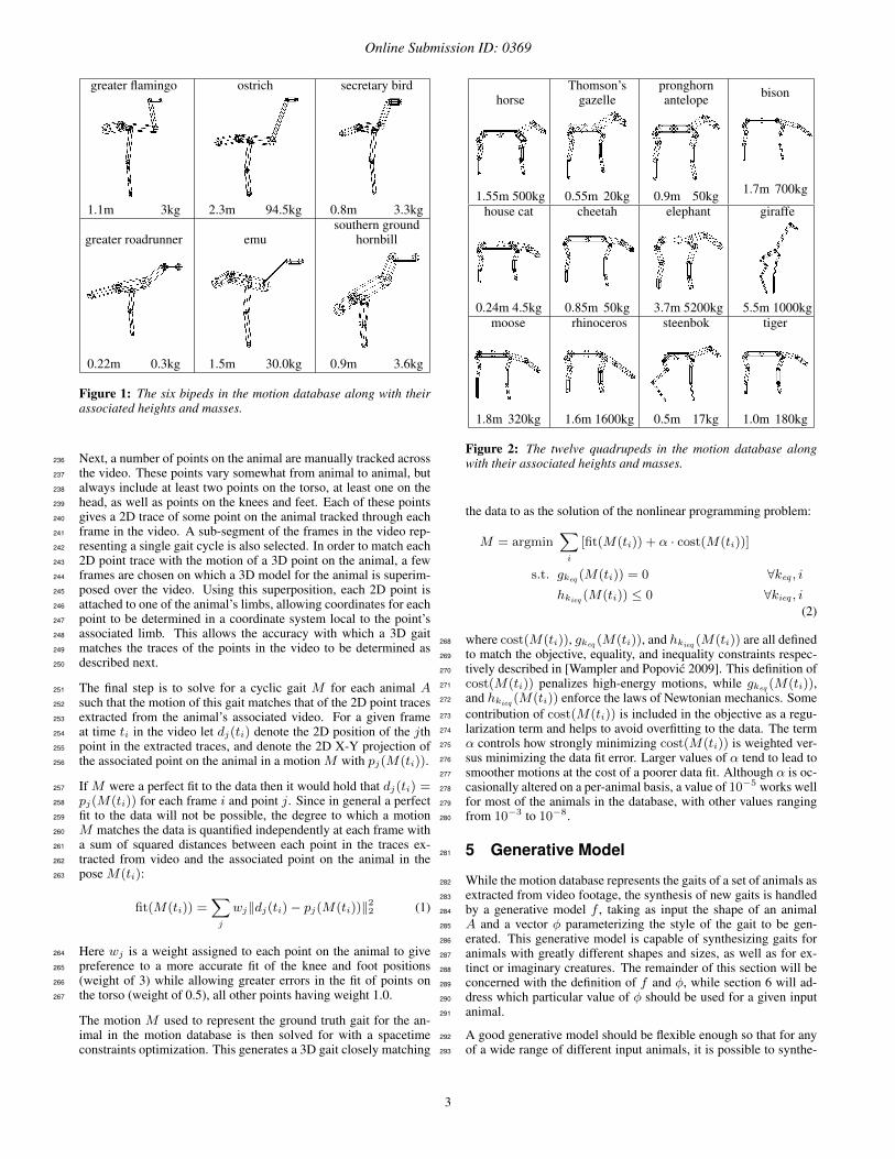
Our motion database consists of six bipeds and twelve quadrupeds226

spanning a wide range of animal shapes and sizes as shown in fig-227

ures 1 and 2. For each of these animals we determine the relative228

lengths and masses of the animal’s limbs by manually constructing229

a crude 3D model from a selected frame in the video, then uni-230

formly scaling each limb’s length and mass so that the animal’s231

height and total mass match the values in figures 1 and 2. For232

each video we also remove the effects of any camera motion by233

translationally stabilizing based on SURF features [Bay et al. 2008]234

tracked between the frames in the video.235

2

Online Submission ID: 0369

greater flamingo

1.1m 3kg

ostrich

2.3m 94.5kg

secretary bird

0.8m 3.3kg

greater roadrunner

0.22m 0.3kg

emu

1.5m 30.0kg

southern groundhornbill

0.9m 3.6kg

Figure 1: The six bipeds in the motion database along with theirassociated heights and masses.

Next, a number of points on the animal are manually tracked across236

the video. These points vary somewhat from animal to animal, but237

always include at least two points on the torso, at least one on the238

head, as well as points on the knees and feet. Each of these points239

gives a 2D trace of some point on the animal tracked through each240

frame in the video. A sub-segment of the frames in the video rep-241

resenting a single gait cycle is also selected. In order to match each242

2D point trace with the motion of a 3D point on the animal, a few243

frames are chosen on which a 3D model for the animal is superim-244

posed over the video. Using this superposition, each 2D point is245

attached to one of the animal’s limbs, allowing coordinates for each246

point to be determined in a coordinate system local to the point’s247

associated limb. This allows the accuracy with which a 3D gait248

matches the traces of the points in the video to be determined as249

described next.250

The final step is to solve for a cyclic gait M for each animal A251

such that the motion of this gait matches that of the 2D point traces252

extracted from the animal’s associated video. For a given frame253

at time ti in the video let dj(ti) denote the 2D position of the jth254

point in the extracted traces, and denote the 2D X-Y projection of255

the associated point on the animal in a motion M with pj(M(ti)).256

If M were a perfect fit to the data then it would hold that dj(ti) =257

pj(M(ti)) for each frame i and point j. Since in general a perfect258

fit to the data will not be possible, the degree to which a motion259

M matches the data is quantified independently at each frame with260

a sum of squared distances between each point in the traces ex-261

tracted from video and the associated point on the animal in the262

pose M(ti):263

fit(M(ti)) =∑j

wj‖dj(ti)− pj(M(ti))‖22 (1)

Here wj is a weight assigned to each point on the animal to give264

preference to a more accurate fit of the knee and foot positions265

(weight of 3) while allowing greater errors in the fit of points on266

the torso (weight of 0.5), all other points having weight 1.0.267

The motion M used to represent the ground truth gait for the an-imal in the motion database is then solved for with a spacetimeconstraints optimization. This generates a 3D gait closely matching

horse

1.55m 500kg

Thomson’sgazelle

0.55m 20kg

pronghornantelope

0.9m 50kg

bison

1.7m 700kg

house cat

0.24m 4.5kg

cheetah

0.85m 50kg

elephant

3.7m 5200kg

giraffe

5.5m 1000kgmoose

1.8m 320kg

rhinoceros

1.6m 1600kg

steenbok

0.5m 17kg

tiger

1.0m 180kg

Figure 2: The twelve quadrupeds in the motion database alongwith their associated heights and masses.

the data to as the solution of the nonlinear programming problem:

M = argmin∑i

[fit(M(ti)) + α · cost(M(ti))]

s.t. gkeq (M(ti)) = 0 ∀keq , ihkieq (M(ti)) ≤ 0 ∀kieq , i

(2)

where cost(M(ti)), gkeq (M(ti)), and hkieq (M(ti)) are all defined268

to match the objective, equality, and inequality constraints respec-269

tively described in [Wampler and Popovic 2009]. This definition of270

cost(M(ti)) penalizes high-energy motions, while gkeq (M(ti)),271

and hkieq (M(ti)) enforce the laws of Newtonian mechanics. Some272

contribution of cost(M(ti)) is included in the objective as a regu-273

larization term and helps to avoid overfitting to the data. The term274

α controls how strongly minimizing cost(M(ti)) is weighted ver-275

sus minimizing the data fit error. Larger values of α tend to lead to276

smoother motions at the cost of a poorer data fit. Although α is oc-277

casionally altered on a per-animal basis, a value of 10−5 works well278

for most of the animals in the database, with other values ranging279

from 10−3 to 10−8.280

5 Generative Model281

While the motion database represents the gaits of a set of animals as282

extracted from video footage, the synthesis of new gaits is handled283

by a generative model f , taking as input the shape of an animal284

A and a vector φ parameterizing the style of the gait to be gen-285

erated. This generative model is capable of synthesizing gaits for286

animals with greatly different shapes and sizes, as well as for ex-287

tinct or imaginary creatures. The remainder of this section will be288

concerned with the definition of f and φ, while section 6 will ad-289

dress which particular value of φ should be used for a given input290

animal.291

A good generative model should be flexible enough so that for any292

of a wide range of different input animals, it is possible to synthe-293

3

Online Submission ID: 0369

size a realistic gait of that animal by an appropriate choice of φ.294

More concretely, for each Ai and Mi in the motion database there295

should be some φi such that Mi ≈ f(Ai, φi). In addition, when296

synthesizing motions for new animals it will be useful for the val-297

ues of φ to be both relatively compact and coherently interpolable298

between different animals.299

Our generative model f is based on the spacetime constraints opti-mization described by [Wampler and Popovic 2009] because of itsability to automatically and relatively quickly synthesize motionsfor a wide range of different animals. In this approach, a motion issynthesized by finding the minimum of a large nonlinear program-ming problem:

f(A, φ) = argminM

∑i

cost(M(ti), φ)

s.t. gkeq (M(ti)) = 0 ∀keq , ihkieq (M(ti)) ≤ 0 ∀kieq , i (3)

Where gkeq and hkieq are the again the equality and inequality con-300

straints enforcing the physical validity of the resulting motion as301

described by [Wampler and Popovic 2009]. In or implementation,302

this optimization is initialized with the animal a default stand-still303

pose and is solved with the SNOPT nonlinear programming library304

[Gill et al. 2005].305

The objective function used in equation 3 dictates which sorts of306

gaits should be preferred over others, and thus altering this objec-307

tive function allows different gaits to be synthesized for the same308

animal. In previous work by [Liu et al. 2005] this idea has been309

used to synthesize different styles of human locomotion by choos-310

ing φ to represent to passive actuation characteristics at the charac-311

ter’s joints. For our task we extend this set to include parameters312

describing the strength and coactuation of different joints, the un-313

certainty of interaction with the ground, and the relative preference314

for low-torque, low-impact, and smooth motions.315

5.1 Generative parameters316

The elements of φ serving as parameters to our generative model arelisted in table 1 and are used to alter the per-frame objective func-tion cost(M(ti), φ) in equation 3. Adjusting the value of φ thusprovides a means by which the style of a synthesized gait can becontrolled. Our choice of generative parameters and the associatedobjective function were found by starting with an objective functionbased purely on torque-minimization, and iteratively adding termsuntil the gaits of the animals within the motion database could bereproduced. The result is a combination of six terms:

cost(M(ti), φ) = costtorque(M(ti), φ)

+ wf costforce(M(ti), φ)

+ wa costsmooth(M(ti), φ)

+ (ewh − 1) costhead(M(ti), φ)

+ costcoactuate(M(ti), φ)

+ (ewg − 1) costground(M(ti), φ) (4)

There are several sub-quantities which must be used to calculate317

these components, all of which are computed as a function of318

M(ti). For notational cleanness, however, we will leave this de-319

pendence on M(ti) implicit and write for instance τ instead of the320

more explicit τ(M(ti)). Accordingly, τ , f , and q will respectively321

represent a vector of the concatenated torques, forces, and joint ro-322

tation angles at each of the character’s joints at the frame M(ti).323

The quantities Rh, ph, and θh will refer to the rotation matrix, posi-324

tion, and angular acceleration for the limb representing the animal’s325

name biped descriptionhg X falloff of ground uncertainty distributionwg X weight for vertical ground penaltieswhg X weight for horizontal ground penaltieshw X maximum height of near-ground dragdw X drag coefficient for near-ground dragcl X weight on knee-ankle coactuationcrl X target ratio for knee vs. ankle velocitiesca weight on elbow-wrist coactuationcra target ratio for elbow vs. wrist velocitiesth X scaling for torques exerted at the hiptk X scaling for torques exerted at the kneeta X scaling for torques exerted at the anklets scaling for torques exerted at the shoulderte scaling for torques exerted at the elbowtw scaling for torques exerted at the wristwf X scaling for joint-force penaltieswa X scaling for joint-acceleration penaltieswh X scaling for head stability penaltiesksh X spring constant for hipqh X spring rest angle for hipkdh X damper coefficient for hipksk X spring constant for kneeqk X spring rest angle for kneekdk X damper coefficient for kneeksa X spring constant for ankleqa X spring rest angle for anklekda X damper coefficient for anklekss spring constant for shoulderqs spring rest angle for shoulderkds damper coefficient for shoulderkse spring constant for elbowqe spring rest angle for elbowkde damper coefficient for elbowksw spring constant for wristqw spring rest angle for wristkdw damper coefficient for wrist

Table 1: A table of the inverse parameters used to specify the styleof an animal’s gait. Quadrupedal animals make use of the wholeset of parameters, while bipeds make use only of those marked.

head as measured about its center of mass. Similarly, pf represents326

the position of a foot. Any temporal derivatives represented by a327

superscript dot are computed using finite differences.328

The first three components of the objective function in equation 4penalize torques, forces, and angular accelerations at the animal’sjoints:

costtorque(M(ti), φ) = wj · τ (5)costforce(M(ti), φ) = wj · f (6)

costsmooth(M(ti), φ) = ‖q‖2 (7)

where wj is a vector of weights with elements equal to eth − 1,329

etk−1, eta−1, ets−1, ete−1, or etw−1 at indices corresponding330

to the hip, knee, ankle, shoulder, elbow or wrist joints respectively.331

All other elements in wj are fixed equal to 1. Lower settings of332

an element in w approximates the effect of ‘stronger’ joints, which333

are actuated by stronger muscles and better able to withstand large334

forces.335

The term costhead(M(ti), φ) penalizes motion in the animal’s headand is computed as the sum of four sub-terms respectively penaliz-ing the rotation of the head away from forward, its velocity, linear

4

Online Submission ID: 0369

acceleration, and angular acceleration:

costhead(M(ti), φ) = (8)

100‖Rh − I‖22 + 2.5‖p2hyz‖22 + ‖ph‖22 + ‖θh‖22

The weights 100 and 2.5 scaling the first two sub-terms where cho-336

sen empirically. Although costhead(M(ti), φ) does not depend on337

φ, the strength with which it factors into equation 4 is scaled by338

(ewh − 1). The term phyz represents the motion of the head in the339

vertical and lateral directions. The function costhead is useful in340

modeling the fact that animals often take additional effort to stabi-341

lize their head motion to help with visual perception.342

The standard spacetime constraints formulation used to synthe-343

size motions treats each joint in the animal as being capable of344

moving entirely independently of all the other joints. In reality,345

however, some pairs of joints exhibit a tendency to be coactu-346

ated such that their motions occur in concert rather than indepen-347

dently. Rather than directly modeling the muscles responsible for348

this as in [Wang et al. 2012], we take a simplified approach where349

costcoactuate(M(ti), φ) penalizes deviations of the relative veloci-350

ties of the animal’s knee and ankle joints from crl :351

(ecl − 1)(crl qk − qa)2 (9)

Where qk and qa are the rotational velocities at the knee and ankle352

respectively. For a quadruped the parameters ca and cra are used to353

add an analogous additional penalty related to the relative velocities354

of the elbow and wrist joints.355

In the optimization defined by equation 3, the animal is implicitly356

assumed to have perfect knowledge of its environment. In real-357

ity this is of course not the case, and in order to avoid tripping an358

animal will often lift its feet higher than is strictly energetically op-359

timal. Since explicitly modeling this uncertainty as in [Wang et al.360

2010] is difficult within a spacetime constraints formulation, we in-361

stead use the term costground(M(ti), φ) to penalize motions where362

the animal’s foot moves quickly while too close to the ground as:363

costground(M(ti), φ) =∑f

pcx‖pfxz‖2 + max{

0,−pcy pfy

}(10)

where the sum is taken over each of the animal’s feet and pfxz andpfy represent the horizontal and vertical components of the foot’svelocity. The values pcxz and pcy approximate the probability ofan ‘unexpected’ contact between the foot and the ground due to thefoot’s horizontal and vertical motion respectively, calculated as:

pcx = whg (1− e−hgpfy ) (11)

pcy =e−hgp

[2]fy − e−hgpfy

1− e−hgpfy(12)

The value p[2]f indicates the position of the foot in the next frame in364

the motion, i.e. pf(M(ti+1)).365

In addition to the term costground(M(ti), φ) directly penalizing366

motions where the foot skirts too close to the ground, we also indi-367

rectly penalize such motions by approximating the resistive forces368

on the leg resulting from walking through shallow water or near-369

ground vegetation. For each foot f , we add a force f resisting the370

foot’s velocity based on the speed of the foot and it’s depth below371

the height defined by hw:372

f = −pf‖pf‖2 max{

0, hw − pfy

}edw (13)

In practice, we have found the effects of this near-ground resistance373

are useful in conjunction with those from costground(M(ti), φ) to374

shape the trajectory of the animal’s feet during their air phases.375

Finally, we include a number of parameters modeling the passive376

actuation characteristics of the animal’s leg joints. for each of377

the hip, knee, ankle, shoulder, elbow, and wrist joints we include378

three parameters specifying a spring rest length, spring constant,379

and damper coefficient for the joint. The use of these parameters is380

identical to that in [Liu et al. 2005], where they were successfully381

used to capture stylistic variations in human locomotion.382

6 Joint Inverse Optimization383

The motion database provides a reference for the real-world gaits of384

a number of different animals, but to create gaits for new animals it385

is necessary to generalize beyond those contained within the motion386

database. While the generative model f(A, φ) described in section387

5 is capable of synthesizing new motions given an animal A and a388

vector of parameters φ, it remains to be determined which value of389

φ is likely to lead to a realistic motion for a given animal.390

We achieve this by fitting a vector φi of parameters to each Mi in391

the motion database. Although we can fit each φi independently,392

we find that the resulting parameters do not allow us to predict393

the motion of new animals. Instead, we propose a new algorithm394

termed joint inverse optimization which jointly learns all of the φi395

together. The resulting parameters are constructed to allow φ to396

be determined for a new animal by simple interpolation. In the re-397

mainder of this section we will first look more closely at the naıve398

case of independently fitting each φi. We will then introduce our399

algorithm of joint inverse optimization, followed by details on its400

implementation.401

6.1 Naıve Inverse Optimization402

As its name implies, joint inverse optimization is based on the ap-403

proach of inverse optimization that has been previously employed404

in character animation [Liu et al. 2005; Lee and Popovic 2010].405

One possible formulation of an inverse optimization problem as ap-406

plied to animal gaits would determine the φi parameters for each407

(Ai,Mi) in the motion database by solving:408

φi = argminφ

D(f(Ai, φ),Mi) (14)

Where the function D(Ma,Mb) defines a distance metric repre-409

senting in the error in how closely the motion Ma matches Mb.410

See section 6.2.1 for the specifics of the distance function used in411

our implementation.412

The problem with using a standard inverse optimization formula-413

tion to determine the φi parameters for each entry in the motion414

database comes when trying to estimate the φnew which will lead415

to a realistic motion for a new animal. In particular, since equation416

14 solves for each φi independently, there is no guarantee of any417

consistency of these parameters between different animals. Indeed,418

as illustrated in figure 3 the φi parameters found using this method419

do not form any easily describable coherent pattern. This makes the420

use of sparse data interpolation to determine which φnew should be421

used to synthesize a gait for a new animal Anew problematic, and422

our attempts to synthesize plausible gaits for new animals using this423

approach were almost entirely unsuccessful.424

6.2 Joint Inverse Optimization425

Because the end goal of our approach is to use the examples in the426

motion database to determine how a new animal should move, we427

explicitly incorporate this requirement into our joint inverse opti-428

mization formulation. The result is an optimization which not only429

attempts to fit each φi with its associated motionMi, but which also430

5

Online Submission ID: 0369

Figure 3: Plots of the values of a parameter for each of thequadrupedal animals in the motion database. The y-axis of eachof the two plots is the value of the te parameter (see table 1) foreach animal while the x-axis represents the logarithm of each ani-mal’s mass. The top plot shows the parameter values resulting fromnaıve inverse optimization while the bottom plot shows the results ofa joint-inverse optimization. The parameters resulting from joint-inverse optimization are substantially better suited to regression.Note that distances along the x-axis are only an approximation tothe similarity of the animals as measured by equation 21, so a per-fectly smooth curve should not be expected in the lower plot.

minimizes a term ensuring that the result is well-suited to sparse431

data interpolation:432

argminθ,φ1,...,φn

∑i

[D(f(Ai, φi),Mi) + β

(‖φi −R(Ai, θ)‖22 + r(θ)

)](15)

This formulation differs from traditional inverse optimization433

(equation 14) by the addition of two functions: A regression func-434

tion and a regularization function. The regression functionR(A, θ)435

takes as input an animal A (not necessarily in the motion database)436

and a vector of regression parameters θ, and returns a vector of437

generative parameters φ suitable for using to synthesize a gait for438

A. The regularization function r(θ) is then used in preventing an439

overfitting of the regression parameters θ. It is the vector of regres-440

sion parameters θ which determines the motion of a new animal441

Anew, by first calculating φnew = R(Anew, θ), then solving for the442

final motion with f(Anew, φnew).443

Intuitively, the goal of a joint inverse optimization is to find a value444

of the regression parameters θ which simultaneously accurately re-445

produces each motion in the motion database via minimizing each446

D(f(Ai, R(Ai, θ)),Mi), and which avoids overfitting by mini-447

mizing r(θ). Unfortunately, the optimization resulting from at-448

tempting to directly minimize this quantity is extremely brittle due449

to the compounding factor that the generative function f is not guar-450

anteed to converge to a physically valid result, and thus for many451

values of θ there are some animals in the motion database for which452

D(f(Ai, R(Ai, θ)),Mi) is impossible to evaluate.453

The formulation for joint inverse optimization given in equation 15454

provides a more robust and efficient approach. In this approach,455

the φi parameters used to solve for an animal’s motion are allowed456

to differ from the parameters resulting from the regression function457

R(Ai, θ). In essence, although the φ parameters used to synthesize458

a gait for a new animal will be found via φnew = R(A, θ), this459

is treated as a soft constraint for the purposes for fitting θ to the460

motion database.461

When accounting for the possibility that f(Ai, φi) might fail to462

converge to a physically valid result, note that in equation 15 the463

only term which relies on the result of the generative model is464

D(f(Ai, φi),Mi). The fact that this term can be computed in-465

dependently for each animal makes it substantially easier to create466

an optimization which solves equation 15 by simply discarding any467

failed evaluations of f(Ai, φi). Our approach for achieving this468

(including the values used for the term β) is described in section469

6.2.3, but we will first provide the specific definitions of D, R, and470

r which we employ.471

6.2.1 Gait distance metric472

Solving the joint inverse optimization problem defined by equation15 requires a definition of D(Ma,Mb), describing a distance met-ric between different gaits. Although a simple sum-or-squared dif-ferences in the rotational degrees of freedom of the animal’s jointsover the course of the two gaits gives reasonable results, we havefound that more visually pleasing results can be obtained with aslightly more involved definition. Intuitively, this is because someaspects of a motion, such as the height by which the feet are raisedor the stability of the head, are more visually important than theprecise angles of rotation for the animal’s joints. We computeD(Ma,Mb) as a sum of per-frame costs, each computed as:

D(Ma(ti),Mb(ti)) =

‖0.25w · (q(Mb(ti))− q(Ma(ti))) ‖22+ (16)

‖0.6w · (q(Mb(ti))− q(Ma(ti))) ‖22+ (17)

‖0.5w · (q(Mb(ti))− q(Ma(ti))) ‖22+ (18)

2.25∑f

(pf (Mb(ti))y − pf (Ma(ti))y)2+ (19)

3.25∑

h∈{h1,h2}

‖ph(Mb(ti))− ph(Ma(ti))‖22+ (20)

Where q(M(ti)) is a vector of the rotational degrees of freedom473

inM at frame i, and ph1(M(ti)), ph2(M(ti)) give the position of474

the front and back of the head at frame i. Similarly, for each foot475

f , pf (M(ti)) gives the position of the foot at frame i. The vector476

w is used to scale the weight given to differences in the rotations at477

different joints. For bipeds w is 2 for the knee and 3 for ankle joints478

while for quadrupeds w is 3 for the knee/elbow joints and and 10479

for the ankle/wrist joints. All other elements in w are set to 1.480

6.2.2 Regression and Regularization Functions481

A joint inverse optimization additionally requires definitions for the482

regression and regularization functions R(Ai, θ) and r(θ). In our483

implementation we use a relatively simple formulation based on484

regression with radial basis functions regularized with quadratic485

smoothing [Boyd and Vandenberghe 2004]. This approach em-486

ploys a definition of θ which concatenates θ1, . . . , θn for each of487

the n animals in the motion database, where each θi has the same488

dimension as the generative parameters φi.489

The distance metric underlying the radial basis function interpola-tion measures the dissimilarity between two animals Aa and Abwith a weighted combination of the difference of the log-masses ofthe two animals and the difference in the lengths of their variouslimbs normalized by the total size of each animal:

d(Aa, Ab)2 =∑

i

(lai∑j laj

− lbi∑j lbj

)2

+ 0.002(ln(ma)− ln(mb))2

(21)

6

Online Submission ID: 0369

where laj and laj are the lengths of the jth limbs in Aa and Ab490

respectively, and ma and mb are the total respective masses of Aa491

andAb. The logarithmic scaling of the masses captures the fact that,492

for instance, a 10kg difference in mass is much more meaningful493

between a 10kg and a 20kg animal than between a 1000kg and a494

1010kg animal.495

Using this distance metric, the regression function is then defined496

in a manner similar to [Zhang et al. 2004] as:497

R(A, θ) =

∑i θie

−d2i∑i e−d2i

(22)

where di = d(A,Ai)dmin

with dmin = mini

d(A,Ai). Here θi are the498

regression parameters directly associated withAi (which in general499

need not be equal to φi due the decoupling of θ from φ1, . . . , φn in500

equation 15).501

To avoid overfitting, we employ a regularization function based on502

quadratic smoothing:503

r(θ) =∑i

‖R(Ai, θ′)− θi‖22 (23)

where θ′ are the regression parameters omitting the θi parameters504

associated with Ai, so this regularization function essentially com-505

putes a sum of leave-one-out errors.506

Finally, the period pi of an animal’s gait cycle and the speed vi atwhich it should move are determined with a separate method by:

pi = αpmiβp (24)

vi = αvllegiβv (25)

In these equations mi is the total mass of and llegi is the average507

length of the legs of Ai. Additionally, αp and βp are parameters508

used to model the relationship between an animal’s mass and the509

period of its gait cycle, while αv , and βv are parameters mod-510

eling relationship between the length of the animal’s legs and its511

speed. The parameters αp, βp, αv , and βv are found from the mo-512

tion database using a least-squares fit. Because the animals in our513

motion database do not exhibit significant differences in the timings514

for their foot contacts once normalized for period and speed, we fix515

the relative timings for the foot contacts in all synthesized gaits to516

match those of a default walk.517

6.2.3 Numerical Solution518

In order to solve the joint inverse optimization problem defined by519

equation 15, we first note that the optimization is in a form which is520

partially decoupled. In particular, only the ‖φi−R(Ai, θ)‖22+r(θ)521

regression error term relates the different animals to each other522

(via θ), and that remaining termD(f(Ai, φi),Mi) can be indepen-523

dently evaluated for each φi. This leads to an optimization tech-524

nique in which a series of otherwise independent optimizations for525

each φi are coupled together by the regression function R(Ai, φ)526

and the regularization function r(θ). This is achieved in a manner527

reminiscent of coordinate descent by alternating between minimiz-528

ing θ and minimizing φ1, . . . , φn.529

Our approach to minimizing equation 15 involves a set of coupled530

instances of the covariance matrix adaptation (CMA) algorithm531

[Hansen et al. 1996]. We maintain a separate mean and covariance532

matrix to solve for for each φi, denoted µi and Ci respectively. At533

the beginning of each iteration a fixed number of samples φi,1, φi,m534

(we use m = 64 in our tests) is drawn for each φi distributed ac-535

cording to µi and Ci. Treating these samples as the current esti-536

mates for each φi, equation 15 is minimized for θ while holding all537

method mean error median errordefault 0.495 0.435kinematic interpolation 0.451 0.387naıve inverse interpolation 0.473 0.360joint-inverse interpolation 0.327 0.245(base inverse fit) 0.142 0.127

Table 2: The mean and median errors over the combined biped andquadruped motion databases of leave-one-out tests in which oneanimal was excluded and its gait synthesized based on the otheranimals. The errors are measured using metric given by equations16-20. Note that the cheetah and emu were excluded from thesestatistics because the ‘naıve inverse interpolation’ spacetime con-straints optimization failed to converge for them.

φi,1, φi,m fixed. As only the ‖φi − R(Ai, θ)‖22 + r(θ) term de-538

pends on θ, solving for θ reduces to a straightforward regularized539

least-squares optimization and can be solved relatively efficiently540

either with an off-the-shelf unconstrained optimizer (or with a sin-541

gle linear least squares solve for appropriate choices of R and r).542

This yields a new estimate for θ, and allows the cost associated543

with each φi,j sample to be computed as defined by equation 15,544

after which the mean µi and covariance Ci associated with eachAi545

are independently updated using the standard CMA update [Hansen546

et al. 1996] omitting any samples for which f(Ai, φi,j) fails.547

Solving a joint inverse optimization problem also requires a setting548

for the parameter β used to weight the terms in the objective func-549

tion resulting from how closely each φi matchesR(Ai, θ). Because550

lower values of β tend to converge more quickly, a continuation is551

performed where β is started out at a low value and then gradually552

increased over the course of the optimization. For quadrupeds we553

set the value of β in iteration i to βi = 0.01 + 0.02 i over a total of554

50 iterations while for bipeds we use βi = 0.001 + 0.004 i over a555

total of 35 iterations.556

7 Results557

We demonstrate our approach of animal gait synthesis using joint558

inverse optimization on a motion database of walking gaits for six559

bipeds and twelve quadrupeds as illustrated in figures 1 and 2.560

Although in principle could use both the bipeds and quadrupeds561

simultaneously, for simplicity we automatically select whether to562

synthesize a motion using only the bipeds or only the quadrupeds563

depending of whether the input animal is a biped or a quadruped.564

Processing this motion database with the joint inverse optimization565

algorithm takes several days when run on a cluster of 96 computers,566

but need only be done once. Synthesizing a gait for a new animal567

once the motion database has been preprocessed takes only a few568

minutes.569

In order to quantitatively compare our approach with other alterna-570

tives, table 2 shows the result of a leave-one-out cross-validation571

for several potential synthesis techniques, including ours:572

default The gait is synthesized using a fixed default value of φi for573

all animals.574

kinematic interpolation The gaits in the motion database are di-575

rectly interpolated weighted according to equation 22. The576

resulting motion will generally not satisfy the laws of physics,577

so a final spacetime constraints optimization is performed578

which attempts to match the kinematic interpolation as closely579

as possible while satisfying the laws of physics.580

naıve inverse interpolation The gait is synthesized using param-581

eters interpolated using equation 22, but without any joint in-582

7

Online Submission ID: 0369

verse optimization (i.e. the generative parameters for each583

animal are optimized independently).584

joint-inverse interpolation Our proposed approach in which a585

gait is synthesized using parameters interpolated using equa-586

tion 22 with joint inverse optimization.587

(base inverse fit) For comparison, each gait is synthesized using588

the optimal independently-fit inverse parameters. In contrast589

to the other approaches listed here this one does make use of590

the ground-truth motion of the animal and is thus analogous591

to the approach of [Liu et al. 2005]. Although this approach592

gives the least error, it is fundamentally incapable of synthe-593

sizing motions for new animals.594

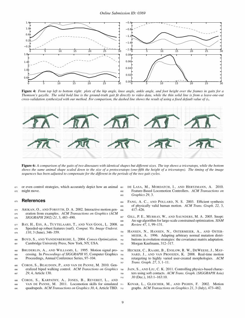
We also illustrate a comparison of the values of the foot height and595

several DOFs for the ground truth and leave-one-out synthesized596

gaits for the Thomson’s gazelle in figure 4. As shown in table 2 our597

approach based on joint inverse optimization outperforms all of the598

other techniques we have tested. In addition, since our generative599

function only requires the shape of an animal and a vector of rela-600

tively general parameters, it is potentially better suited to creating601

a range of different motions for an animal as in [Liu et al. 2005]602

than an approach based on kinematic interpolation from the motion603

database.604

We have also tested our approach on synthesizing gaits for a number605

of extinct animals, including land-birds, mammals, and dinosaurs.606

Even when the shape of the animals differs significantly from any-607

thing in the motion database (or even from anything currently liv-608

ing) the gaits appear to be visually reasonable. A snapshot of these609

motions appears in figure 5. We also have found that the synthe-610

sized gaits adjust in a visually reasonable manner to the size of the611

animal. For example, figure 6 shows gaits for two dinosaurs with612

the same relative shape but different total sizes. The synthesized613

gaits are significantly different, and on a qualitative level capture614

the sort of differences which would be expected considering the615

triceratops’ substantially greater size and mass. Of course in these616

cases there is no possibility of a ‘ground truth’ motion to validate617

these synthesized gaits against. Nevertheless, the synthetic gaits618

still provide a compelling glimpse at how these creatures might619

have walked.620

There are a couple of situations where our proposed method does621

not perform as well. The first of these situations is when little data622

exists for a type of animal in the motion database. For instance, our623

motion database contains only three cats, and the the leave-one-out624

cross-validation for these motions shows an error greater than for625

the other animals in the database. The second situation in which this626

method can perform poorly is when large extrapolations are used.627

For instance the motions synthesized for a paraceratherium (four628

times the mass of an elephant) or for argentinosaurus huinculensis629

(4.5 times the mass of an elephant) exhibit some over-bending of630

the legs which is probably not realistic. Extrapolating further to631

the motion of a amphicoelias fragillimus (20 times the mass of an632

elephant) yields clearly unrealistic results. Nevertheless, when used633

on animals with a size near those in the motion database, the method634

given here performs well, even if the shape of the animal itself is635

relatively unlike anything currently living.636

8 Conclusion637

We have presented a technique for learning a model representing638

the style of walking gaits for a range of different animals, then us-639

ing this model to synthesize gaits for new animals. Our method is640

based on a novel algorithm called joint inverse optimization which641

learns coherent patterns underlying the gaits of different animals.642

This allows the synthesis of visually plausible gaits for a variety643

Figure 5: The top illustrates the gaits synthesized for a number ofextinct mammals and lan- birds, while the bottom shows the gaitssynthesized for a several dinosaurs. In the bottom image a giraffeappears in the background for size comparison.

of different extinct creatures, and has been verified to be superior to644

several other techniques at estimating the gaits of a range of animals645

for which we do have data.646

There are of course a great number of ways in which our work647

could be improved in the future. Perhaps the simplest of these is648

in the creation of a larger and more detailed motion database. Al-649

though we have achieved satisfactory results with a relatively small650

database extracted from 2D video footage, it is likely that the use651

of 3D motion capture and force plates could further improve the re-652

sults. Our approach also does not perform well when extrapolating653

gait style onto animals with a shape vastly different than anything654

we have data for. Although we expect that a more faithful biome-655

chanical model of each animal may help with this as in [Wang et al.656

2012], it remains an open question just what the most useful biome-657

chanical factors to include would be. In addition, our approach uses658

simple RBF-based interpolation to determine the style of a new an-659

imal, but it is likely that a more sophisticated regression technique660

could be better suited to large extrapolations.661

On a more theoretical level, our approach captures variations in662

style between different animals, but cannot account for the multi-663

tude of different motions often performed by even a single animal.664

This is because we treat the style of an animal’s gait as fixed by the665

shape of the animal. Instead, it would be fruitful for future tech-666

niques to be able to model the set of styles likely to be exhibited in667

the motions of an animal with a given shape. Even further in this di-668

rection, an ideal method would not be limited to just gait synthesis,669

but would be able to produce a diverse range of realistic motions,670

8

Online Submission ID: 0369

Figure 4: From top left to bottom right: plots of the hip angle, knee angle, ankle angle, and foot height over the frames in gaits for aThomson’s gazelle. The solid bold line is the ground-truth gait fit directly to video data, while the thin solid line is from a leave-one-outcross-validation synthesized with our method. For comparison, the dashed line shows the result of using a fixed default value of φi.

Figure 6: A comparison of the gaits of two dinosaurs with identical shapes but different sizes. The top shows a triceratops, while the bottomshows the same animal shape scaled down to the size of a protoceratops (one-fifth the height of a triceratops). The timing of the imagesequences has been adjusted to compensate for the different in the periods of the two gait cycles.

or even control strategies, which accurately depict how an animal671

might move.672

References673

ARIKAN, O., AND FORSYTH, D. A. 2002. Interactive motion gen-674

eration from examples. ACM Transactions on Graphics (ACM675

SIGGRAPH 2002) 21, 3, 483–490.676

BAY, H., ESS, A., TUYTELAARS, T., AND VAN GOOL, L. 2008.677

Speeded-up robust features (surf). Comput. Vis. Image Underst.678

110, 3 (June), 346–359.679

BOYD, S., AND VANDENBERGHE, L. 2004. Convex Optimization.680

Cambridge University Press, New York, NY, USA.681

BRUDERLIN, A., AND WILLIAMS, L. 1995. Motion signal pro-682

cessing. In Proceedings of SIGGRAPH 95, Computer Graphics683

Proceedings, Annual Conference Series, 97–104.684

COROS, S., BEAUDOIN, P., AND VAN DE PANNE, M. 2010. Gen-685

eralized biped walking control. ACM Transctions on Graphics686

29, 4, Article 130.687

COROS, S., KARPATHY, A., JONES, B., REVERET, L., AND688

VAN DE PANNE, M. 2011. Locomotion skills for simulated689

quadrupeds. ACM Transactions on Graphics 30, 4, Article TBD.690

DE LASA, M., MORDATCH, I., AND HERTZMANN, A. 2010.691

Feature-Based Locomotion Controllers. ACM Transactions on692

Graphics 29, 3.693

FANG, A. C., AND POLLARD, N. S. 2003. Efficient synthesis694

of physically valid human motion. ACM Trans. Graph. 22, 3,695

417–426.696

GILL, P. E., MURRAY, W., AND SAUNDERS, M. A. 2005. Snopt:697

An sqp algorithm for large-scale constrained optimization. SIAM698

Review 47, 1, 99–131.699

HANSEN, N., HANSEN, N., OSTERMEIER, A., AND OSTER-700

MEIER, A. 1996. Adapting arbitrary normal mutation distri-701

butions in evolution strategies: the covariance matrix adaptation.702

Morgan Kaufmann, 312–317.703

HECKER, C., RAABE, B., ENSLOW, R. W., DEWEESE, J., MAY-704

NARD, J., AND VAN PROOIJEN, K. 2008. Real-time motion705

retargeting to highly varied user-created morphologies. ACM706

Trans. Graph. 27, 3, 1–11.707

JAIN, S., AND LIU, C. K. 2011. Controlling physics-based charac-708

ters using soft contacts. ACM Trans. Graph. (SIGGRAPH Asia)709

30 (Dec.), 163:1–163:10.710

KOVAR, L., GLEICHER, M., AND PIGHIN, F. 2002. Motion711

graphs. ACM Transactions on Graphics 21, 3 (July), 473–482.712

9

Online Submission ID: 0369

KRY, P. G., REVERET, L., FAURE, F., AND CANI, M.-P. 2009.713

Modal locomotion: Animating virtual characters with natural vi-714

brations. Computer Graphics Forum.715

LEE, S. J., AND POPOVIC, Z. 2010. Learning behavior styles with716

inverse reinforcement learning. ACM Trans. Graph. 29, 4, 1–7.717

LEE, J., CHAI, J., REITSMA, P. S. A., HODGINS, J. K., AND718

POLLARD, N. S. 2002. Interactive control of avatars animated719

with human motion data. ACM Transactions on Graphics 21, 3720

(July), 491–500.721

LIU, C. K., HERTZMANN, A., AND POPOVIC, Z. 2005. Learning722

physics-based motion style with nonlinear inverse optimization.723

ACM Trans. Graph. 24, 3, 1071–1081.724

MORDATCH, I., DE LASA, M., AND HERTZMANN, A. 2010. Ro-725

bust physics-based locomotion using low-dimensional planning.726

ACM Transactions on Graphics 29, 4 (July), 71:1–71:8.727

MORDATCH, I., TODOROV, E., AND POPOVIC, Z. 2012. Dis-728

covery of complex behaviors through contact-invariant optimiza-729

tion. ACM Trans. Graph. 31, 4 (July), 43:1–43:8.730

NUNES, R. F., CAVALCANTE-NETO, J. B., VIDAL, C. A., KRY,731

P. G., AND ZORDAN, V. B. 2012. Using natural vibrations732

to guide control for locomotion. In Proceedings of the ACM733

SIGGRAPH Symposium on Interactive 3D Graphics and Games,734

ACM, New York, NY, USA, I3D ’12, 87–94.735

POPOVIC, Z., AND WITKIN, A. 1999. Physically based motion736

transformation. In SIGGRAPH ’99: Proceedings of the 26th737

annual conference on Computer graphics and interactive tech-738

niques, ACM Press/Addison-Wesley Publishing Co., New York,739

NY, USA, 11–20.740

RAIBERT, M. H., AND HODGINS, J. K. 1991. Animation of741

dynamic legged locomotion. SIGGRAPH Comput. Graph. 25742

(July), 349–358.743

SAFONOVA, A., HODGINS, J. K., AND POLLARD, N. S.744

2004. Synthesizing physically realistic human motion in low-745

dimensional, behavior-specific spaces. ACM Trans. Graph. 23,746

3, 514–521.747

WAMPLER, K., AND POPOVIC, Z. 2009. Optimal gait and form748

for animal locomotion. ACM Trans. Graph. 28, 3, 1–8.749

WANG, J. M., FLEET, D. J., AND HERTZMANN, A. 2010. Op-750

timizing walking controllers for uncertain inputs and environ-751

ments. ACM Trans. Graph. 29, 4 (July), 73:1–73:8.752

WANG, J. M., HAMNER, S. R., DELP, S. L., AND KOLTUN,753

V. 2012. Optimizing locomotion controllers using biologically-754

based actuators and objectives. ACM Trans. Graph. 31, 4, 25.755

WEI, X., MIN, J., AND CHAI, J. 2011. Physically valid statistical756

models for human motion generation. ACM Trans. Graph. 30757

(May), 19:1–19:10.758

WITKIN, A. P., AND POPOVIC, Z. 1995. Motion warping. In Pro-759

ceedings of SIGGRAPH 95, Computer Graphics Proceedings,760

Annual Conference Series, 105–108.761

YIN, K., LOKEN, K., AND VAN DE PANNE, M. 2007. Simbicon:762

Simple biped locomotion control. ACM Trans. Graph. 26, 3,763

Article 105.764

ZHANG, L., SNAVELY, N., CURLESS, B., AND SEITZ, S. M.765

2004. Spacetime faces: High-resolution capture for modeling766

and animation. In ACM Annual Conference on Computer Graph-767

ics, 548–558.768

10